WP020-08 Finance and - BRACIL for Computational Finance and Economic Agents Working Paper Series WP020-08 Philip Saks Dietmar Maringer Statistical Arbitrage with ... Statistical Arbitrage

Centre forComputationalFinance andEconomicAgents

WorkingPaperSeries

www.essex.ac.uk/ccfea

WP020-08

Philip SaksDietmar Maringer

Statistical Arbitrage withGenetic Programming

May 2008

Statistical Arbitrage with Genetic Programming

Philip Saks∗ Dietmar Maringer

May 5, 2008

Abstract

This paper employs genetic programming to discover statistical arbi-trage strategies on the banking sector in the Euro Stoxx universe. Binarydecision rules are evolved using two different representations. The first isthe classical single tree approach, where one decision tree for buy and sellorders is developed. The second version uses a dual tree structure wheretwo decision trees are generated and the evaluation is contingent on thecurrent market position. Hence, buy and sell rules are co-evolved for longand short positions. Applied to empirical high-frequency prices for stocksof banking companies, both methods are capable of discovering significantstatistical arbitrage strategies, even in the presence of realistic market im-pact. This implies the existence of market inefficiencies within the chosenuniverse. However, the performance of the successful strategies deteriorateover time and the inefficiencies have disappeared in the second half of theout-of-sample period.

As transaction costs are increased there is a clear asymmetric responsebetween single and dual trees. Naturally, increased costs have a negativeimpact on performance, but the dual trees are much more robust and canadapt to the changed environment, whereas the single trees cannot.

1 Introduction

During the last decades, the Efficient Market Hypothesis (EMH) has been put to

trial, especially with the emergence of behavioral finance and agent-based com-

putational economics. The rise of the above mentioned fields provides a theoret-

ical justification for attacking the EMH, which in turn stimulates the empirical

forecasting literature.

A basic premise for efficiency is the existence of homo economicus, that the

markets consists of homogeneous rational agents, driven by utility maximization.

However, cognitive psychology has revealed that people are far from rational, in-

stead they rely on heuristics in decision making to simplify a given problem [17].

∗both: Centre for Computational Finance and Economic Agents, University of Essex, Wivenhoe

Park, Colchester CO4 3SQ, UK. {psaks,dmaring}[at℄essex.a .uk. The authors are grateful for

valuable comments and suggestions by conference and seminar participants in Cambridge, Naples

and Essex. Financial support from the EU Commission through MRTN-CT-2006-034270 COMISEF

is gratefully acknowledged.

1

1 Introduction 2

This is both useful and necessary in everyday life, but in certain situations it

can lead to biases such as overconfidence, base-rate neglect, sample-size neglect,

gamblers fallacy, conservatism and aversion to ambiguity [3]. What is more im-

portant is that these biases manifest themselves on an aggregate level in the mar-

kets as momentum and mean-reversion effects [14, 7]. Accepting the existence

of heterogenous agents have pronounced effects on a theoretical level. In such a

scenario the market clearing price cannot be determined formally, since agents

need to form expectations about other agents’ expectations. This leads to an “in-

finite regress in subjectivity” where agents cannot form expectations by deduc-

tive means, regardless of their reasoning powers. Thus perfect rationality is not

well-defined. Instead, investors are forced to hypothesize expectational models

where the only means of verification is to observe the models’ performance in

practice [2]. In such a world it is indeed sensible to develop expectational mod-

els beyond traditional equilibrium analysis. In this paper, such models are built

using genetic programming (GP).

The majority of existing applications of GP in financial forecasting have fo-

cused on foreign exchange. Here, the general consensus is that GP can dis-

cover profitable trading rules at high frequencies in presence of transaction costs

[16, 9, 6]. For the stock market results are mixed. The buy-and-hold strategy on

daily S&P500 data is not outperformed [1], while it is on a monthly frequency

[5]. Besides changing the frequency, a reduced grammar is considered. More-

over, buy and sell rules are co-evolved separately.

In this paper, we consider genetic programming for statistical arbitrage. Ar-

bitrage in the traditional sense is concerned with identifying situations where a

self-funding is generated that will provide only non-negative cash flows at any

point in time. Obviously, such portfolios are possible only in out-of-equilibrium

situations. Statistical arbitrage is a wider concept where, again, self-funding

portfolios are sought where one can expect non-negative pay outs at any point

in time. Here one accepts negative pay-outs with a small probability as long as

the expected positive payouts are high enough and the probability of losses is

small enough; ideally this shortfall probability converges to zero. In practice,

such a situation can occur when price processes are closely linked. In the clas-

sical story of Royal Dutch and Shell [3], the pair of stocks are cointegrated due

to their fundamental link via their merger in 1907. In most cases, however, such

links are not as obvious, but that does not eliminate the possibility that such rela-

tionships might exist and can be detected by statistical analysis. In the following

stocks within the same industry sector are considered, since it can be argued that

these stocks are exposed to many of the same risk factors and should therefore

have similar behavior.

As mentioned previously, an arbitrage portfolio is constructed by using the

proceedings from short selling some stocks to initiate long positions in other

stocks. More formally, the cumulative discounted value (vt ) of a statistical arbi-

P Saks, D Maringer, Statisti al Arbitrage with Geneti Programming, CCFEA WP 020-08, Universityof Essex 2008.

2 Clustering of Financial Data 3

trage strategy has to satisfy the following conditions [13],

v0 = 0 (1)

limt→∞

E(vt)> 0 (2)

limt→∞

prob(vt < 0)= 0 (3)

limt→∞

V ar (vt)

t= 0 if prob(vt < 0)> 0 ∀t <∞ (4)

This means that it has to have zero initial cost and be self-financing (1); a positive

discounted value (2); and a probability of loss converging to zero (3). Condition

(4) states that a statistical arbitrage produces riskless incremental profits in the

limit.

By taking relative value bets between highly correlated stocks from the same

industry, much of the market uncertainty is hedged away. Hence, profits made

from this strategy are virtually uncorrelated with the market index. Further-

more, by modeling the relationships between stocks, the attention is focused on

a direction where more stable patterns should exist rather than making specific

predictions about future developments. This statement defies the EMH in its

weakest form, that no trading system based on historical price and volume infor-

mation should generate excess returns [10].

The rest of the paper is organized as follows. Section 2 analyzes the Euro

Stoxx universe and provides evidence of significant clustering between sectors.

Section 3 introduces the data, model and framework. Sections 4 and 5 present

results under the assumptions of frictionless trading and realistic market impact,

respectively. In Section 6 the transaction cost is gradually increased and the ef-

fects on the single and dual trees are investigated. Finally, Section 7 concludes

and gives pointers to possible future research.

2 Clustering of Financial Data

It is frequently argued that stocks within the same industry sector are exposed

to many of the same risk factors and should therefore have similar behavior. In

order to clarify this, we investigate the majority of stocks in the Euro Stoxx 600

index. The data is gathered from Bloomberg and includes information such as

company name, ticker symbol, industry sector and industry group. In addition

hereto, we obtain the adjusted closing prices in the period from 21-Jan-2002 to

26-Jun-2007. Since the index composition is changing over time, we only con-

sider stocks where data exists for the last two years for both price and volume

series. Taking this into account, the universe comprises of a total of 477 stocks.

The notion that stocks have similar behavior needs to be specified in order to

conduct a proper analysis. An obvious measure for price data is the correlation

of returns, where a higher correlation implies stronger similarity. Figure 1 shows

the maximum spanning tree for the undirected graph defined by the upper tri-

angle of the return’s correlation matrix, adjusted for country effects - in practice

we estimate the minimum spanning tree, where the correlations are transformed,P Saks, D Maringer, Statisti al Arbitrage with Geneti Programming, CCFEA WP 020-08, Universityof Essex 2008.

2 Clustering of Financial Data 4

AABA NA

AAL LN

ABBN VX

ABF LN

ALPHA GAAC FP

ADEN VX

ADS GY

AGN NA

AEM IM

AGS LN

AH NA AF FP

AI FPAKZA NA

AL/ LN

ALBK ID

ALFA SS

ALT GY

ALU FP

ALV GY

AL IM

AMEC LNANGL ID

ANTO LNARI LN

ARM LN

ASML NA

ASSAB SS

ATCOA SS

ATO FP

AV/ LN

CS FP

AZN LN

BA/ LN

BAER VX

BALN VX

BARC LN

BAS GY

BATS LN

BAY LN

BAY GY

BB/ LN

BBA LN

BBY LN

BELG BB

BCP PL

BDEV LNBEI GY

BESNN PL

BG/ LN

BGY LN

BKG LN

BKIR ID

BLND LN

BLT LN

BMPS IM

BMW GY

BNP FP

BNZL LN

BOB FP

TELL GA

TPEIR GA

EN FPBP/ LN

BPIN PL

BRE LN

BRISA PL

BSY LNBT/A LN

BUL IM

BVS LN

BWY LN

BXTN LN

ACA FP

CAP FP

CARLB DC

CA FPCO FP

CASS IM

CAST SSCBG LN

CBK GY

CBRY LN

CCL LN

CFR VX

CGCBV FHCIBN VX

CLN VX

CLS1 GY

CNA LN

KN FP

CNE LN

CNP FP

COB LN

COLOB DC

CON GY

CORA NA

COSMO GA CPG LN

CPI LN

CIMP PLCAP IM

UC IM

CRG IM

CRH ID

CSGN VX

CSMNC NA

CTT LN

CW/ LN

BN FPDANSKE DC

DSY FP

DB1 GY

DBK GY

DCC ID

DCO DC

PPC GA

DEP GY

DEXB BB

DGE LNCDI FP

DMGT LN

DNBNOR NO

DPB GYDPW GY

DSGI LN

DSM NA

DSV DC

DTE GY

EAD FP

ECM LN

EDP PL

EUROB GA

ELI1V FH

ELN ID

REN NA

ELUXB SS

EMA LN

EMG LN

ENEL IM

ENI IM

ENRO SS

EOA GY

ERICB SS

EBS AV

EF FP

ETI LN

RF FP

SW FP

FABG SS

FGP LN

F IM

FME GY

FORA NA

FSA IM

FGR FP

FP/ LN

FRE3 GY

FTE FP

FUM1V FH

FWB IM

G IM

GETIB SS

GFC FP

GFS LN

GIVN VX

GKN LN

GN DC

GNK LN

GN5 ID

GSK LN

HAS LN

HBOS LN

HDD GYHEI GYHEIA NA HEIO NA

EEEK GA

HMSO LN

HMB SS

HEN3 GY

HNR1 GY

HNS LN

HOLMB SS

HOLN VX

HOT GY

RMS FP

HRX GY

HSBA LN

IAP LN

IAW ID

ICI LN

ICP LN

IFX GY

IHG LN

III LN

IIA AV

IMI LN

IMT LN

NK FP

INCH LN

INDUA SS

INF LN

INGA NA

INB BB

INVEB SS

INVP LN

INWS ID

IPM ID

IPR LN

ISP IM

ISYS LN

IT IM

ITRK LN

ITV LN

DEC FP

JMAT LN

JPR LN

JYSK DC

KEL LN

KESA LNKESBV FH

KGF LNKINVB SS

KNEBV FH

KPN NA

KSP ID

KYG ID

LAD LN

LG FP

MMB FP

LAND LN

LGEN LN

LHA GY

LII LN

LIN GY

LLOY LN

LMI LN

LOG LN

LI FP

LONN VX

LSE LN

LUX IM

MC FP

SZE FP

MAB LN

MAERSKB DC

MAN GY

MARS LN

MB IM

MED IM

MEO1V FH

MEO GY

MGGT LN

ML FP

MKS LN

MMT FP

MRK GY

MRW LN

MS IM

MOBB BB

MSY LN

MTGB SS

MUV2 GY

MF FPETE GA

NDA SS

NES1V FH

NESN VX

NEX LN

NG/ LN

NHY NO

NOK1V FH

NOVN VX

NOVOB DC

NEO FP

NRK LN

NSG NONUM NA

NWG LN

NXT LN NZYMB DC

OML LN

OMV AV

OPAP GAOR FP ORK NO

HTO GA

OUT1V FH PAJ FP

PC IM

RI FP

UG FP

PFG LN

PG IM

PHIA NA

BPM IM

PNN LN

PP FP

PRU LNPOR3 GY

PSM GY

PSN LN

PSON LN

PTC PL

PUB LN

PUB FP

PUM GY

QIA GY

RAND NA

RB/ LNRBS LN

REL LN

RNO FP

REX LN

RHM GY

RIBH AV

RIO LN

ROG VX

RR/ LN

RSA LN

RSL LN

RTO LN

RTR LN

RUKN VX

RWE GY

RYA ID

SAB LN

SAF FP

SAMAS FH

SAND SS

SAP GYSAN FP

SBMO NA

SBRY LN

SCAB SS

SU FP

SCMN VX

SCTN LN

SCVB SS

SDF GY

SDR LN

SEBA SS

SECUB SS

SESG FPSGC LN

SGE LN DG FPSGO FP

SGSN VX

SHBA SS SHP LN

SIE GY

FNC IM

SIG LN

SKAB SSSKFB SS

SLHN VX

SMIN LN

SN/ LNGLE FP

SPM IM

SRG IM

SRP LN

SSABA SS

SSE LN

SAZ GY

STAN LNSTB NO

STERV FH

STL NO

STM IM

SVT LN

SWEDA SS

SWMA SS

SWS1V FH

SYDB DC

SYNN VX

SYST VX

TATE LN

HO FP

TEC FP

TEL NO

TEL2B SS

TKA AV

TFI FP

TIE1V FH

TKA GY

TIT IMTLSN SS

TLW LN

TMS FP

TNI LN

TNT NA

TOMK LN

TOP DC

FP FP

TPK LN

TRELB SS

TRN IM

TSCO LN

TITK GA

UBM LNUBSN VX

UHR VX

ULVR LN

UL FP

UNA NA

UPM1V FH

UU/ LN

VDOR NA

VIE FP

VIV FP

FR FP

VOD LN

VOE AV

VOLVB SSVOW GY

VWS DC

WIE AV

WHA NA

WLSNC NA

WMH LN

WOS LN

WPP LN

WRTBV FH

WTB LN

XTA LN

YAR NO

YELL LN

YTY1V FH

ZC FP

ZURN VX

ABE SQ

ACS SQ

ACX SQ

ALB SQ

ALT SQ

ANA SQ

ATLN SE

BBVA SQ BKT SQBVA SQ

CIN SQ

ELE SQ

ENG SQ

EVA SQ

FCC SQ

FER SQ

GAM SQ

GAS SQ

GEBN SE

IBE SQ

IDR SQ

ITX SQ

KNIN SELISN SE

LOGN SE

MAP SQ

MVC SQ

PARG SE

POP SQ

PSPN SE

REE SQ

REP SQ

SAB SQ

SAN SQ

SCHP SE

SGC SQ

SIK SE

SYV SQ

TEF SQ

TL5 SQUBI IM

UNF SQ

ZOT SQ

Basic Materials

Communications

Consumer, Cyclical

Consumer, Non-cyclical

Diversified

Energy

Financial

Industrial

Technology

Utilities

Figure 1: Maximum spanning tree of Euro Stoxx 600 correlation matrix (graph

created with Pajek)

ρi , j → |ρi , j −1|. An undirected graph is a collection of vertices and edges, and

a spanning tree is a subgraph in which all the vertices are connected. In our

case, each vertex represents a stock, and we have a fully connected graph where

the edges comprise of the transformed correlations. This measure can be viewed

as the cost of linking two stocks, and the minimum spanning tree is simply the

spanning tree which connects all the nodes, such that the combined cost is mini-

mal. The minimum spanning tree is unique, given each edge has a distinct weight

and can be estimated efficiently using the greedy Kruskal’s algorithm.

The color of the vertices represents the industry sector and it appears that

there is a pronounced clustering, especially for the basic material, communica-

tion and financial sector. It is worth noting that retail giants such as Unilever

(UNA NA), Nestle (NESN VX) and Cadbury Schweppes (CBRY LN) are tightly

linked. Another interesting feature is that three major basic material stocks are

connected: BHP Billiton (BLT LN), Rio Tinto (RIO LN) and Antofagasta (ANTO

LN). This is not surprising since these stocks in addition to being in the same

industry sector, also share the same industry group, mining.P Saks, D Maringer, Statisti al Arbitrage with Geneti Programming, CCFEA WP 020-08, Universityof Essex 2008.

3 Framework 5

The maximum spanning tree merely provides a graphical representation of

the relationships within the index, but is not in itself a statistical test for the

hypothesis that stocks within a sector tend to be clustered together. Clustering

analysis is nothing novel within statistics, and various methods such as the k-

means algorithm can efficiently tackle this problem. Thus, if the statistical clus-

tering is independent of the fundamental clustering, dictated by the industry sec-

tors, then one can reject the hypothesis. Let S and F be two stochastic variables

which describe the statistical and fundamental clusters, respectively. The statis-

tical clusters are obtained by using k-means on the correlation matrix, while the

fundamental cluster are built according to the industries the assets belong to. The

maximum values they can attain is denoted by the integers ks and k f . If N is the

number of stocks in the universe, the hypothesis of independence can be tested

by computing

V j ,m =

N∑

i=1

I{si= j } · I{ fi=m} ∀ j = 1,2, . . . ,ks m = 1,2, . . . ,k f (5)

via a χ2 statistic for contingency tables. Setting ks = k f = 10, this test statistic is

χ2 = 1314.1 while the critical value is χ20.05(81) = 103.0; hence, thus strongly re-

jecting the null hypothesis that statistical and fundamental clusters are indepen-

dent. In other words, significant clustering within the sectors can be expected,

and it is reasonable to pre-select assets from one fundamental cluster (here: be-

longing to the same industry) for the actual statistical arbitrage application.

3 Framework

As mentioned previously, the objective is to develop a trading strategy for statis-

tical arbitrage based on price and volume information, and in the following we

elaborate on data, preprocessing and model construction.

3.1 Data

The data comprises of Volume-Weighted Average Prices (VWAP) and volume,

sampled at an hourly frequency for the banks in the Euro Stoxx 600 index. It cov-

ers the time period from 01-Apr-2003 to 29-Jun-2007, corresponding to a total of

8648 observations. Again, we only consider stocks for which we have enough

data, which limits the portfolio to 30 assets. The components and summary

statistics are documented in Table 7 and the VWAP prices are depicted in Fig-

ure 2.

When analyzing high frequency data, it is important to take intraday effects

into account. Figure 3 shows the average intraday volume for ABN AMRO in the

period from 04-Jul-2006 to 29-Jun-2007. Clearly, the volume is higher after open

and before close than during the middle of the day. In the context of trading rule

induction it is important to remove this bias, which is basically a proxy for the

time of day, and prohibits reasonable conditioning on intraday volume.P Saks, D Maringer, Statisti al Arbitrage with Geneti Programming, CCFEA WP 020-08, Universityof Essex 2008.

3 Framework 6

2003 2004 2004 2005 2005 2006 2006 2007

101

102

103

Banking Stocks

Year

Figure 2: Hourly VWAP prices for banking stocks within the Euro Stoxx index

0606

0607

07

8

10

12

14

160

1

2

3

4

5

x 106

Year

Volume Profile, ABN AMRO

Time

Figure 3: Expected intraday volume for ABN AMRO in the period from 17-May-

2007 to 29-Jun-2007P Saks, D Maringer, Statisti al Arbitrage with Geneti Programming, CCFEA WP 020-08, Universityof Essex 2008.

3 Framework 7

3.2 Preprocessing

The return series for each stock is standardized with respect to its volatility, es-

timated using simple exponential smoothing. Likewise, a volume indicator is

constructed that removes the intraday bias, and measures the extent to which the

level is lower or higher than expected. Specifically, we take the logarithm of the

ratio between the realized and expected volume, where this ratio has been hard

limited in the range between 0.2 and 5.

Since the main focus is on cross-sectional relationships between stocks,

rather than their direction, we subtract the cross-sectional average from the nor-

malized returns and volume series for each stock. Based on these series, we calcu-

late the moving averages over the last 8, 40 and 80 periods; at an hourly frequency

this corresponds to one day, a week and two weeks, respectively. All indicators

are transformed to quantiles, using a Gaussian distribution function estimated

on a 3-month rolling window basis.

3.3 Model

There are two approaches for modeling trading rules; either as decision trees

where market positions or actions are represented in the terminal nodes [18], or

as a single rule where the conditioning is exogenous to the program [6].

We consider the latter approach in the context of a binary decision problem,

which corresponds to long and short positions. As mentioned previously, the

focus of this paper is on arbitrage portfolios, where the purchase of stocks is

financed by short selling others. Naturally, a precondition for this is that not all

the forecasts across the 30 stocks are the same. For example if the trading rule

takes a bullish view across the board, then short-selling opportunities have not

been identified and proper arbitrage portfolios cannot be constructed. In this

case no stocks are held. However, when forecasts facilitate portfolio construction,

this is done on a volatility adjusted basis. Let oit ∈ {−1,1} denote the forecast on

stock i at time t , such that -1 and 1 corresponds to a bearish and bullish view,

respectively. Then the holding is given by

hit = oi

t ·

1σi

t∑n

j=11

σjt

· I{o

jt =oi

t }

(6)

where σt is the volatility, n is the number of stocks in the universe, and I{o

jt =oi

t }

is an indicator variable that ensures that forecasts are normalized correctly i.e.

it discriminates between long and short positions. By construction the long and

short positions sum to -1 and 1, respectively.

n∑

j=1

hjt I

{hjt >0}

= 1

n∑

j=1

hjt I

{hjt <0}

= −1 (7)

By down weighting more volatile stocks the portfolio becomes more stable.P Saks, D Maringer, Statisti al Arbitrage with Geneti Programming, CCFEA WP 020-08, Universityof Essex 2008.

3 Framework 8

Function Arguments Return Type<, > (qrtn, q onst) bool<, > (qvol, q onst) boolBTWN (qrtn, q onst, q onst) boolBTWN (qvol, q onst, q onst) boolAND, OR, XOR (bool, bool) boolNOT (bool) boolITE (bool, bool, bool) boolTable 1: Statistical arbitrage grammar, where BTWN checks if the first argument is

between the second and third. ITE represents the if-then-else statement

We employ two different methods for solving the binary decision problem.

The first uses a standard single tree structure, while the second considers a dual

tree structure in conjunction with cooperative co-evolution [4]. In both methods,

the trees return boolean values. For a more rigorous analysis of the dual tree

approach, see Saks and Maringer [20]

For the dual tree structure, program evaluation is contingent on the current

market position for that particular stock, i.e., the first tree dictates the long entry,

while the second enters a short position. In other words, which of these two trees

is evaluated, depends on the previous position; if stock i at time t was in a short

position (oit−1 < 0), then tree k = 1 is evaluated and dictates if a long position

should be initiated. Alternatively, tree k = 2 is evaluated to decide whether to

enter a short position. Let bk ,it ∈ {0,1} be the truth value for tree k on stock i at

time t , whether or not to switch positions, then b1,it = 1 (b2,i

t = 1) indicates to

enter a long (short) position, while b1,it = 0 (b2,i

t = 0) leaves the current position

unchanged. Then the new forecast is given as

oit =

{

2 ·b1,it −1 if oi

t−1 < 0

−2 ·b2,it +1 otherwise

(8)

All trees are constructed from the same grammar, which in addition to type

constraints also introduces semantic restrictions. This improves the search ef-

ficiency significantly, since computational resources are not wasted on non-

sensical solutions [6]. We consider a fairly restricted grammar, which is docu-

mented in Table 1. It consists of numeric comparators, boolean operators and

if-then-else statements (ITE). Furthermore, a special function BTWN has been in-

troduced, that takes three arguments and evaluates if the first is between the sec-

ond and third. The terminals comprise of the six indicators where there is a dis-

tinction between return (qrtn) and volume (qvol) information, and numerical

real-valued constants (q onst) ranging from 0 to 1. The parsimonious gram-

mar reduces the risk of overfitting, and enhances interpretability of the evolved

solutions.

The choice of a suitable objective function is essential in evolutionary com-

putation. Previous studies suggest that a risk-adjusted measure improves out-P Saks, D Maringer, Statisti al Arbitrage with Geneti Programming, CCFEA WP 020-08, Universityof Essex 2008.

4 Frictionless Trading 9

of-sample performance when compared to an absolute return measure [6]. In

this context, the ratio between the average profits and their volatility would be

an obvious candidate. However, under this measure strategies might evolve that

do extremely well only on a subset of the in-sample data and mediocre on the

remainder; from a practical point of view, this can lead to additional vulnera-

bility to market timing as the overall success might depend more on the entry

and exit points than on the overall time. Instead, the t-statistic of the linear fit

between cumulated profits and time is employed, since it maximizes the slope

while minimizing the deviation from the ideal straight line performance graph.

This measure favors a steady increase in wealth – Figure 13 in the Appendix illus-

trates this concept.

3.4 Parameter Settings

In the following computational experiments a population of 250 individuals is

initialized using the ramped half-and-half method. It evolves for a maximum of

51 generations, but is stopped after 15 generations if no new elitist (best-so-far)

individual has been found. A normal tournament selection is used with a size

of 5, and the crossover and mutation probabilities are 0.9 and 0.1, respectively.

Moreover, the probability of selecting a function node during reproduction is

0.9, and the programs are constrained to a maximum complexity of 50 nodes.

Again, this constraint is imposed to minimize the risk of overfitting, but also to

facilitate interpretability. If the models lose tractability, it defies the purpose of

genetic programming as a knowledge discovery tool.

The data is split into a training and test set. The former contains 6000 samples

and covers the period from 01-Apr-2003 to 10-Mar-2006, and the latter has 2647

samples in the period from 13-Mar-2006 to 29-Jun-2007.

4 Frictionless Trading

4.1 Performance

As will be discussed in more detail in Section 5, placing a buy or sell order will

have an impact on the market price, in particular on a high frequency level in a

market with continuous auctions. This impact will be smaller for an arbitrarily

small order size in relation to the market volume. For the sake of simplicity,

this section assumes the absence of market impact, i.e., that all placed orders

are executed on the realized volume weighted average price (VWAP). Trading on

the VWAP differs from a traditional market order, where a trade is executed at

the current observed price. The VWAP is a backward looking measure, and it

is therefore not possible to trade on the observed VWAP at time t . Instead the

execution occurs gradually between t and t +1, resulting in the VWAP at t +1. In

summary, a trading decision is formed based on the VWAP at time t , the entry

price is observed at time t +1 and the one period profit is evaluated at t +2.



08/07/03 02/23/04 09/10/04 03/29/05 10/15/05

−0.2

0

0.2

0.4

0.6

0.8

Single tree 0bp, in−sample cumulated profits

Date

Cum

ulat

ed p

rofit

s

08/07/03 02/23/04 09/10/04 03/29/05 10/15/05

−0.2

0

0.2

0.4

0.6

0.8

1

1.2Dual tree 0bp, in−sample cumulated profits

Date

Cum

ulat

ed p

rofit

s05/03/06 08/11/06 11/19/06 02/27/07 06/07/07

−0.2

−0.1

0

0.1

0.2

0.3

0.4

Single tree 0bp, out−of−sample cumulated profits

Date

Cum

ulat

ed p

rofit

s

05/03/06 08/11/06 11/19/06 02/27/07 06/07/07

−0.2

−0.1

0

0.1

0.2

0.3

Dual tree 0bp, out−of−sample cumulated profits

Date

Cum

ulat

ed p

rofit

s

Figure 4: In-sample (top) and out-of-sample cumulated profits (bottom) assum-

ing frictionless trading. The black line is average performance and the 95% and

99% confidence intervals are constructed using the stationary bootstrap proce-

dure. The left and right column are the single and dual tree results, respectively.

We perform 10 experiments using both the single and dual tree method, ac-

cording to the settings outlined in Section 3. For each experiment, the best-so-far

individual is evaluated on the training and test set.

The self-financing property of a statistical arbitrage portfolio implies that its

return in the strict sense is not well defined1. Instead, the log-profits are evalu-

ated at each time period,

pt =

n∑

j=1

rjt ·h

jt (9)

where rjt is the log-return of stock j at time t . Due to the constraint (7), the log-

profit approximates the money amount made from investing one currency unit

on both the long and short side of the portfolio. In the subsequent analysis profits

and wealth, refers to log-profits and log-wealth unless otherwise specified.

Figure 4 shows the growth in wealth for the evolved trading strategies, and Ta-

bles 2 and 3 provide more detailed performance statistics such as the t-statistic

fitness (TF), annualized profits (AP), profit-risk ratios (PRR)2, maximum draw

1The return of an investment is the ratio of terminal to initial wealth (vt /v0 −1), but by defini-

tion v0 = 0 for statistical arbitrage portfolios2This is the average profits divided by their standard deviation.P Saks, D Maringer, Statisti al Arbitrage with Geneti Programming, CCFEA WP 020-08, Universityof Essex 2008.


0.15 0.2 0.25 0.3 0.35 0.4 0.45

0.1

0.15

0.2

0.25

0.3

In−sample

Out

−of

−sa

mpl

e

Single tree 0bp, annualized profit

0.15 0.2 0.25 0.3 0.35 0.4 0.45

0.1

0.15

0.2

0.25

0.3

In−sample

Out

−of

−sa

mpl

e

Dual tree 0bp, annualized profit

Figure 5: Annualized in-sample versus out-of-sample profits with the 45◦-line,

for the single trees (left) and dual trees (right).

down (MDD) and turnover (TO). Casual inspection of the in-sample results re-

veal that the t-statistic measure works as intended, since all strategies have steady

increasing wealth over time. The values range between 945 and 2038 for the single

trees, and 1007 and 2685 for the dual trees. The annualized profits range between

0.212 and 0.327 with an average of 0.270 for the single trees, and 0.185, 0.404 and

0.249 are the equivalent statistics for the dual trees.

In practice a statistical arbitrage strategy require a margin deposited in a

risk-free account. By taking additional exposure in the self financing risky strat-

egy relative to the margin the profits can be scaled to suit investor utility. Hence,

they are merely a function of leverage. The PRR which is leverage invariant is

therefore a more descriptive measure. Here the range is between 2.71 and 4.07 for

the single trees, and 2.78 and 3.69 for the dual trees. Due to the stochastic nature

of genetic programming, the evolved rules are generally different and it is there-

fore possible to improve the performance due to diversification. The aggregated

holdings are simply the average of the holdings for the ten individual strategies.

Under aggregation, the PRRs increase to 4.66 and 5.03, for the single and dual

trees, respectively. Unfortunately, aggregation or bagging destroys any simple

structure of the model, or in other words it, “a bagged tree is no longer a tree”

[12]. Consequently, interpretability is lost, which is clearly a drawback. However,

by bagging the evolved strategies it is possible to make general inferences about

their properties. In this paper all ten evolved strategies are aggregated, but one

could employ various schemes to improve out-of-sample performance. Gener-

ally, this requires the use of additional validation sets, but since data is limited

this is problematic. Moreover, aggregating all strategies is clearly the conserva-

tive approach and is therefore preferred. The worst in-sample drawdowns are

0.103 and 0.075 for the single and dual trees, respectively. Under aggregation

they fall to 0.044 and 0.034.

Another important statistic is the average daily turnover, which measures the

extent to which the portfolio holdings are changing. Formally it is defined as

τ=1

T

T∑

t=1

n∑

i=1

∣

∣

∣∆hit

∣

∣

∣ ∆hit = hi

t −hit−1 hi

0 = 0 (10)P Saks, D Maringer, Statisti al Arbitrage with Geneti Programming, CCFEA WP 020-08, Universityof Essex 2008.


In-sample Out-of-sample

Strategy TF AP PRR MDD TO TF AP PRR MDD TO

1. 1273 0.256 3.61 -0.067 4.43 247 0.194 2.61 -0.041 4.32

2. 1507 0.327 3.28 -0.066 5.43 292 0.316 2.95 -0.090 5.08

3. 1518 0.279 3.70 -0.050 5.96 332 0.220 2.77 -0.040 5.72

4. 1514 0.248 3.77 -0.047 6.86 454 0.211 3.05 -0.033 6.77

5. 1455 0.296 2.22 -0.103 3.95 460 0.255 1.64 -0.140 3.97

6. 1469 0.258 4.07 -0.042 4.18 412 0.203 3.17 -0.038 3.95

7. 1700 0.325 3.98 -0.063 4.02 355 0.209 2.27 -0.047 3.93

8. 945 0.212 2.71 -0.067 2.64 393 0.262 3.27 -0.063 2.73

9. 1629 0.270 3.70 -0.059 3.03 457 0.227 2.98 -0.051 3.02

10. 2038 0.230 3.51 -0.044 5.85 503 0.237 3.60 -0.030 5.69

Aggregate 2306 0.270 4.66 -0.044 3.51 455 0.233 3.92 -0.028 3.43

Out-of-sample, 1st half Out-of-sample, 2nd half


1. 217 0.273 3.35 -0.041 4.29 141 0.115 1.74 -0.041 4.36

2. 367 0.491 4.32 -0.063 5.14 97 0.141 1.41 -0.090 5.01

3. 218 0.264 2.97 -0.040 5.82 259 0.177 2.58 -0.028 5.63

4. 268 0.227 3.05 -0.033 6.83 111 0.196 3.06 -0.019 6.70

5. 190 0.331 2.45 -0.065 4.24 171 0.179 1.03 -0.140 3.70

6. 283 0.244 3.45 -0.038 4.02 153 0.162 2.87 -0.038 3.89

7. 236 0.280 2.66 -0.047 4.08 156 0.138 1.80 -0.036 3.79

8. 357 0.362 4.15 -0.039 2.80 159 0.162 2.24 -0.063 2.67

9. 260 0.292 3.56 -0.051 3.13 187 0.162 2.32 -0.038 2.91

10. 420 0.270 3.89 -0.021 5.70 231 0.203 3.29 -0.030 5.68

Aggregate 490 0.303 4.85 -0.028 3.50 297 0.163 2.90 -0.027 3.36

Table 2: Strategy performance statistics for single trees under frictionless trad-

ing. The following abbreviations are used; TF – t-statistic fitness, AP – annual-

ized profits, PRR – profit-risk ratio, MDD – maximum drawdown, TO – average

daily turnover.

where T is the number of time periods.

In a frictionless environment the turnover is high since there is no cost asso-

ciated with trading. For the single trees it ranges between 2.64 to 6.86, but for the

dual trees the maximum daily turnover is a massive 20.25.

Naturally, the value of a trading strategy is not dictated by its in-sample per-

formance but is assessed out-of-sample. A drawback of the t-statistic measure

is that it is not sample-size invariant, hence out-of-sample and in-sample results

are not comparable. On an aggregate level the TF is 455 and 287 for the single and

dual trees, respectively. The annualized profits for the single trees range between

0.194 and 0.316 with an average of 0.233, while for the dual trees the numbers

are 0.093, 0.262 and 0.199. Likewise, the PRRs vary between 1.64 and 3.60 for the

single trees and, 1.17 and 3.98 for the dual trees.

To investigate the strategies market timing capabilities confidence intervals

are constructed using the stationary bootstrap method, which is a superior al-

ternative to well known block bootstrap procedure [19]. Instead of using aP Saks, D Maringer, Statisti al Arbitrage with Geneti Programming, CCFEA WP 020-08, Universityof Essex 2008.




1. 1639 0.245 3.26 -0.047 16.50 141 0.093 1.23 -0.056 16.12

2. 1007 0.194 3.03 -0.037 9.03 325 0.251 3.98 -0.029 8.96

3. 2685 0.403 3.69 -0.075 16.17 215 0.146 1.17 -0.087 15.16

4. 1378 0.218 2.97 -0.043 12.12 355 0.203 2.62 -0.042 12.19

5. 1578 0.285 3.51 -0.055 10.50 372 0.253 3.13 -0.043 10.15

6. 1318 0.197 2.98 -0.046 8.56 266 0.222 3.47 -0.028 8.45

7. 1540 0.185 2.91 -0.063 5.10 307 0.188 3.01 -0.036 5.06

8. 1873 0.276 3.16 -0.062 20.25 275 0.243 2.88 -0.045 20.25

9. 1330 0.208 3.37 -0.039 11.55 144 0.126 2.00 -0.052 11.10

10. 1272 0.279 2.78 -0.052 19.02 247 0.262 2.44 -0.058 18.75

Aggregate 2691 0.249 5.03 -0.034 6.46 287 0.198 4.02 -0.022 6.39



1. 102 0.152 1.83 -0.053 16.23 2 0.034 0.51 -0.056 16.01

2. 226 0.310 4.73 -0.026 8.88 193 0.192 3.18 -0.029 9.03

3. 181 0.192 1.36 -0.087 15.56 43 0.099 0.95 -0.068 14.76

4. 357 0.283 3.42 -0.042 12.33 139 0.123 1.72 -0.034 12.05

5. 329 0.330 3.74 -0.043 10.00 206 0.176 2.43 -0.030 10.29

6. 190 0.303 4.41 -0.028 8.35 55 0.141 2.39 -0.028 8.55

7. 218 0.251 3.83 -0.026 5.04 109 0.125 2.12 -0.036 5.07

8. 193 0.303 3.30 -0.045 20.18 55 0.182 2.41 -0.033 20.33

9. 250 0.233 3.44 -0.026 10.98 -17 0.019 0.32 -0.052 11.22

10. 331 0.405 3.33 -0.044 18.49 88 0.119 1.32 -0.058 19.01

Aggregate 330 0.276 5.10 -0.022 6.63 165 0.121 2.75 -0.016 6.16

Table 3: Strategy performance statistics for dual trees under frictionless trading.

The following abbreviations are used; TF – t-statistic fitness, AP – annualized

profits, PRR – profit-risk ratio, MDD – maximum drawdown, TO – average daily

turnover.



fixed block size, it varies probabilistically according to a geometric distribution3 .

Thus, sampling with replacement is performed from the strategy holdings, and

statistics are gathered from 500 runs. For the single tree method all (10/10) strate-

gies exceed the 99% upper confidence limit, while only 7/10 do amongst the dual

trees.

Despite good overall out-of-sample performance, Figure 4 reveals that it is

deteriorating as a function of time. To examine this in more detail, Tables 2 and

3 report the out-of-sample performance statistics on two sub-periods, from 13-

Mar-2006 to 02-Nov-2006 and from 02-Nov-2006 until 29-Jun-2007. In the first

half, both the single and dual trees generalize extremely well obtaining average

annualized profits of 0.303 and 0.276, which actually exceeds their in-sample per-

formances. Furthermore, it is worth noting that the TFs on an aggregate level are

considerably higher than average TFs of the individual strategies. In the second

period the average APs are approximately halved to 0.164 and 0.121 for the sin-

gle and dual trees, respectively. A similar conclusion is reached by analyzing the

profit-risk ratios.

Positive out-of-sample performance need not imply market inefficiency. Tra-

ditionally, this is investigated by comparing the trading strategy to the buy-and-

hold strategy, i.e., a passive long only portfolio. This, however, is not a suitable

benchmark for statistical arbitrage strategies. This is mainly because a statisti-

cal arbitrage is self-financing and the buy-and-hold is not. Obviously one could

short the risk-free asset and invest in the proceeds in an equally weighted portfo-

lio of the underlying stocks4, but this is a naive approach contingent on a specific

equilibrium model. In benchmarking this gives rise to the joint hypothesis prob-

lem, that abnormal returns need not imply market inefficiency, but can be due to

misspecification of a given equilibrium model [11]. Another benchmark which

closer to the spirit of the statistical arbitrage application presented in this paper,

is based on the idea that stocks exhibit momentum [14]. Based on the in-sample

returns, a portfolio is formed by selling (buying) the bottom (top) quintile with

respect to performance. In the out-of-sample period this portfolio generates an

annualized profit of 0.069 and has a PRR of 0.61, but its maximum drawdown is

a substantial 0.157. This is clearly inferior to both the single and dual trees.

A better alternative to these types of benchmarks is to employ a special sta-

tistical test for statistical arbitrage strategies, which circumvents the joint hy-

pothesis problem [13]. The constant mean version of the test assumes that the

discounted incremental profits5 satisfy,

∆vi =µ+σiλzi i = 1,2, . . . ,n (11)

3The probability parameter p = 0.01, generate blocks with an expected length of 100 samples4This benchmark has an annualized profit of 0.045, and a PRR of 0.35 in the out-of-sample

period.5As a discount rate we employ the 1-month LIBOR rate for the Eurozone. The profits are made

from investing one currency unit in both the long and short positions, but they are not com-

pounded, instead they are invested in a risk-free account. Hence, proportionally less are invested

in the risky strategy over time.P Saks, D Maringer, Statisti al Arbitrage with Geneti Programming, CCFEA WP 020-08, Universityof Essex 2008.

5 Market Impact 15

where zi ∼ N (0,1). The joint hypothesis, H1 : µ > 0 and H2 : λ < 0 determines

the presence of statistical arbitrage. The p-values for the joint hypothesis are

obtained via the Bonferroni inequality6

Tables 8 and 9 report the test statistics over the full- and two halves of the

out-of-sample period. Among the single trees 9/10 have discovered a significant

statistical arbitrage based on the entire sample on a 0.05 level of significance. As

was previously documented the performance deteriorates in the second half and

none are significant anymore. For the dual trees 8/10 are significant over the full

sample, but again none are during the second half.

Despite rejection of the null hypothesis it is premature to conclude the exis-

tence of market inefficiencies, since trading costs have not been taken into ac-

count. Specifically, “prices reflect information to the point where the marginal

benefits of acting on information (the profits to be made) do not exceed the

marginal costs” [15]. Hence, in the following the unrealistic assumption of fric-

tionless markets is relaxed.

5 Market Impact

5.1 Performance

The previous section assumed frictionless trading, but in practice trading is as-

sociated with market impact. The slippage depends on the order size relative to

the liquidity of the stock and the time horizon over which the VWAP is executed.

A good execution algorithm is capable of targeting the VWAP within one basis

point for moderate order sizes7. In the following, trading strategies are evolved

in the presence of realistic market impact.

The introduction of transaction costs obviously has an adverse effect on per-

formance. The graphs in Figure 6 display the cumulated profits over time for the

individual strategies both in- and out-of-sample, and Tables 4 and 5 contain the

performance statistics of the individual strategies.

In-sample, the aggregate TF is 1651 and 1143 for the single and dual trees,

respectively. This is considerably less than their frictionless counterparts. The

annualized profits for the single trees range between 0.168 and 0.300 and have an

average of 0.221. The dual trees fair worse and range in the interval from 0.056 to

0.223 with an average of 0.135. Likewise the profit-risk ratios deteriorate under

frictions and range between 1.97 and 2.69 for the single trees. Again, aggregation

results in model diversification and the PRR increases to 3.12. For the dual trees it

ranges between 0.72 and 2.86, and is 3.02 on an aggregate level. Not surprisingly,

the maximum drawdowns in-sample are also higher, i.e. 0.114 and 0.099 for the

single and dual trees, respectively. For the bagged models they are reduced to

0.073 and 0.038.

6prob(⋃n

i=1Ai ) É

∑ni=1

prob(Ai ). The Bonferroni inequality provides an upper bound for the

likelihood of the joint event, by simply summing the probabilities for the individual events without

subtracting the probabilities of their intersections.7Lehman Brothers Equity Quantitative Analytics, London.P Saks, D Maringer, Statisti al Arbitrage with Geneti Programming, CCFEA WP 020-08, Universityof Essex 2008.

5 Market Impact 16

08/07/03 02/23/04 09/10/04 03/29/05 10/15/05

−0.4

−0.2

0

0.2

0.4

0.6

0.8

Single tree 1bp, in−sample cumulated profits

Date

Cum

ulat

ed p

rofit

s

08/07/03 02/23/04 09/10/04 03/29/05 10/15/05−0.4

−0.2

0

0.2

0.4

0.6

Dual tree 1bp, in−sample cumulated profits

Date

Cum

ulat

ed p

rofit

s

05/03/06 08/11/06 11/19/06 02/27/07 06/07/07−0.4

−0.3

−0.2

−0.1

0

0.1

0.2

0.3

Single tree 1bp, out−of−sample cumulated profits

Date

Cum

ulat

ed p

rofit

s

05/03/06 08/11/06 11/19/06 02/27/07 06/07/07

−0.3

−0.2

−0.1

0

0.1

0.2

0.3

Dual tree 1bp, out−of−sample cumulated profits

Date

Cum

ulat

ed p

rofit

s

Figure 6: In-sample (top) and out-of-sample cumulated profits (bottom) assum-

ing a market impact of 1bp. The black line is average performance and the 95%

and 99% confidence intervals are constructed using the stationary bootstrap pro-

cedure. The left and right column are the single and dual tree results, respectively.

0 0.05 0.1 0.15 0.2 0.25 0.30

0.05

0.1

0.15

0.2

0.25

In−sample

Out

−of

−sa

mpl

e

Single tree 1bp, annualized profit

0 0.05 0.1 0.15 0.2 0.25 0.30

0.05

0.1

0.15

0.2

0.25

In−sample

Out

−of

−sa

mpl

e

Dual tree 1bp, annualized profit

Figure 7: Annualized in-sample versus out-of-sample profits with the 45◦-line,

for the single trees (left) and dual trees (right).


5 Market Impact 17



1. 1324 0.250 2.64 -0.089 3.91 256 0.166 1.54 -0.089 3.75

2. 1368 0.254 2.68 -0.072 4.51 198 0.107 1.00 -0.088 4.36

3. 1257 0.300 2.45 -0.082 5.37 55 0.003 0.03 -0.157 5.07

4. 979 0.215 2.67 -0.060 3.03 177 0.036 0.40 -0.076 2.95

5. 1065 0.225 2.36 -0.085 3.65 259 0.215 2.02 -0.077 3.71

6. 909 0.168 2.60 -0.053 2.94 227 0.127 1.95 -0.053 2.81

7. 1349 0.221 2.69 -0.078 4.08 219 0.144 1.56 -0.051 4.05

8. 963 0.190 1.97 -0.114 3.18 288 0.127 1.11 -0.101 3.03

9. 909 0.168 2.60 -0.053 2.94 227 0.127 1.95 -0.053 2.81

10. 1205 0.224 2.38 -0.098 4.18 286 0.091 0.89 -0.073 4.10

Aggregate 1651 0.221 3.12 -0.073 2.98 274 0.114 1.48 -0.058 2.88



1. 181 0.278 2.28 -0.059 4.04 81 0.053 0.58 -0.089 3.45

2. 170 0.256 2.17 -0.058 4.53 35 -0.042 -0.45 -0.088 4.20

3. 20 0.071 0.46 -0.157 5.27 -15 -0.064 -0.57 -0.082 4.88

4. 67 0.035 0.35 -0.043 2.90 82 0.038 0.46 -0.076 3.00

5. 316 0.385 3.56 -0.048 3.90 79 0.044 0.43 -0.077 3.52

6. 235 0.206 3.01 -0.053 2.86 38 0.047 0.77 -0.046 2.75

7. 228 0.233 2.22 -0.048 4.21 51 0.054 0.70 -0.051 3.88

8. 98 0.186 1.65 -0.073 3.24 107 0.067 0.58 -0.101 2.82

9. 235 0.206 3.01 -0.053 2.86 38 0.047 0.77 -0.046 2.75

10. 96 0.114 1.02 -0.056 4.41 103 0.067 0.74 -0.073 3.78

Aggregate 214 0.197 2.41 -0.038 3.00 82 0.031 0.44 -0.058 2.76

Table 4: Strategy performance statistics for single trees under 1bp market impact.



turnover.

A more interesting feature is the effect of transaction costs on the turnover.

For the single trees there is a slight decrease and it ranges between 2.94 and 5.37,

and in aggregate it is 2.98. For the dual trees the effects are substantial. Under

frictionless trading 7/10 strategies had a daily turnover above 10, in the presence

of market impact it ranges between 0.46 and 3.03 with an aggregate value of 1.19.

Out-of-sample the single trees have quite a diverse performance with TFs

ranging from 55 to 288 with an aggregate value of 274. The annualized prof-

its range from 0.003 to 0.215, with an average of 0.114. Analyzing each half of

the test period, it becomes clear that the majority of the performance can be at-

tributed to the first half, where the aggregate annualized profit is 0.197 versus an

unimpressive 0.031 in the second half. The PRRs are in the interval from 0.03 to

2.02, and on aggregate it is 1.48. Moreover, from the first to the second half of

the out-of-sample period it drops from 2.41 to 0.44. With such a negative impact

on the profit-risk ratios, it is not surprising that the maximum drawdown for a

strategy increases to 0.157, however on aggregate it is only 0.058 which is actually

smaller than the in-sample statistic of 0.073.P Saks, D Maringer, Statisti al Arbitrage with Geneti Programming, CCFEA WP 020-08, Universityof Essex 2008.

5 Market Impact 18



1. 439 0.140 2.14 -0.050 1.16 237 0.120 1.77 -0.036 1.11

2. 821 0.148 2.25 -0.059 1.30 105 0.058 0.85 -0.077 1.24

3. 824 0.209 2.05 -0.084 2.58 249 0.161 1.45 -0.058 2.41

4. 289 0.062 0.96 -0.086 2.38 141 0.087 1.39 -0.074 2.41

5. 1775 0.223 2.86 -0.049 1.31 128 0.071 0.95 -0.076 1.08

6. 379 0.056 0.72 -0.099 3.03 26 0.016 0.22 -0.074 2.96

7. 827 0.096 1.53 -0.067 0.70 43 0.022 0.34 -0.071 0.61

8. 802 0.128 1.91 -0.062 1.66 352 0.243 3.56 -0.045 1.63

9. 1219 0.143 2.31 -0.046 0.68 311 0.122 1.95 -0.040 0.65

10. 1320 0.148 2.46 -0.043 0.46 476 0.175 2.76 -0.030 0.42

Aggregate 1143 0.135 3.02 -0.038 1.19 263 0.107 2.41 -0.026 1.13



1. 139 0.162 2.16 -0.036 1.08 103 0.077 1.31 -0.028 1.14

2. 132 0.118 1.56 -0.042 1.21 -0 -0.002 -0.04 -0.076 1.27

3. 123 0.222 1.88 -0.046 2.45 9 0.100 0.96 -0.058 2.38

4. 169 0.142 2.12 -0.038 2.53 2 0.032 0.56 -0.074 2.29

5. 193 0.196 2.49 -0.038 1.08 -19 -0.054 -0.78 -0.076 1.07

6. 23 0.010 0.13 -0.060 2.92 4 0.022 0.31 -0.068 3.01

7. 36 0.008 0.13 -0.052 0.63 32 0.036 0.56 -0.052 0.59

8. 155 0.267 3.54 -0.045 1.57 122 0.219 3.64 -0.022 1.69

9. 124 0.158 2.30 -0.040 0.64 124 0.086 1.55 -0.031 0.66

10. 199 0.196 2.77 -0.030 0.41 174 0.153 2.79 -0.027 0.42

Aggregate 208 0.148 3.03 -0.023 1.14 95 0.067 1.67 -0.026 1.13

Table 5: Strategy performance statistics for dual trees under 1bp market impact.



turnover.


5 Market Impact 19

The maximum TF for the dual trees is 476, which is clearly better than that of

the single trees, but on aggregate they perform approximately the same according

to this measure. From a profit perspective they seem to generalize much better,

and on average the annualized profit only decreases from 0.135 in-sample to 0.107

out-of-sample. However, among the individual strategies there are considerable

variation in performance from 0.016 to 0.243, and the PRRs vary from 0.22 to

3.56, with an aggregate value of 2.41. Contrary to the single-trees the maximum

drawdowns are much more homogeneous and varies between 0.030 and 0.077.

On aggregate it is 0.026, which almost one-third the value of the single trees. In

the first half of the test period, the dual trees perform extremely well and have

an average annualized profit of 0.148 which is superior to the in-sample result.

In the second half, performance deteriorates again and is on average 0.067, albeit

the best performing strategy still manage an impressive 0.219.

To assess the market timing, confidence intervals are again constructed us-

ing the stationary bootstrap. In a frictionless environment a random forecaster

makes on average a zero return, but in the presence of transaction costs we see

that there is a slight negative drift. At the end of the out-of-sample period, 8/10

single trees and 5/10 dual trees exceed the 99% upper confidence limit, and it

must be concluded that they have significant forecasting power.

The essential question remains whether significant statistical arbitrage

strategies have been uncovered. Tables 10 and 11 provide the statistics for the sta-

tistical arbitrage test [13]. For entire out-of-sample period, 2/10 single trees and

5/10 dual trees reject the null hypothesis at a 0.05 level of significance. Likewise,

both aggregate models constitute significant statistical arbitrage strategies. For

the first half of the out-of-sample period, 4/10 single trees and 7/10 dual trees are

significant. During the second half none of the strategies are significant. Based

on these observations it must be concluded that the markets are not efficient in

this high frequency domain. However, it also holds that these inefficiencies dis-

appear over time, or rather, that a static model can only be expected to have a

limited lifespan in a dynamic market.

5.2 Decomposition & Timing

A unique feature of statistical arbitrage strategies is the equity market neutral

constraint, i.e., the long and short positions outbalance each other. To gain fur-

ther understanding of the portfolios it is instructive to decompose the profits

from the long and the short side. Figure 8 shows this decomposition. During the

in-sample period the market has a phenomenal bull run and appreciates with ap-

proximately 90%, which implies that the short positions are loss making for both

the single and dual trees. The long side, however, outperforms the market by up

to 50%. Naturally, in this scenario financing via the riskless asset would a better

option than short selling the stocks. The problem is that this strategy requires

knowledge about the market direction ex ante.

The out-of-sample period contains the crash of May 2006, during which the

short side makes money and prevents a large drawdown which would otherwise

have occurred with cash financing. By hedging the long side using highly corre-P Saks, D Maringer, Statisti al Arbitrage with Geneti Programming, CCFEA WP 020-08, Universityof Essex 2008.

5 Market Impact 20

08/07/03 02/23/04 09/10/04 03/29/05 10/15/05

−0.5

0

0.5

1

1.5

Date

Cum

ulat

ed p

rofit

s

Single tree 1bp, in−sample decomposition

08/07/03 02/23/04 09/10/04 03/29/05 10/15/05

−0.5

0

0.5

1

Date

Cum

ulat

ed p

rofit

s

Dual tree 1bp, in−sample decomposition

05/03/06 08/11/06 11/19/06 02/27/07 06/07/07

−0.1

0

0.1

0.2

0.3

Date

Cum

ulat

ed p

rofit

s

Single tree 1bp, out−of−sample decomposition

05/03/06 08/11/06 11/19/06 02/27/07 06/07/07

−0.1

0

0.1

0.2

0.3

Date

Cum

ulat

ed p

rofit

s

Dual tree 1bp, out−of−sample decomposition

Figure 8: Decomposition of the profits from the long (blue) and short positions

(red). The green line is the buy-and-hold performance of an equally weighted

portfolio of banking stocks and the black line is the aggregate strategies perfor-

mance. Single trees (left) and dual trees (right)


5 Market Impact 21

0 5 10 15 20 25 300

0.01

0.02

0.03

0.04

0.05

0.06

0.07

0.08

Pro

port

ion

Stock

Single tree 1bp, long stock allocation

0 5 10 15 20 25 300

0.01

0.02

0.03

0.04

0.05

0.06

0.07

0.08

Stock

Pro

port

ion

Dual tree 1bp, long stock allocation

Figure 9: Conditional distribution of long positions across stocks. Single trees

(left) and dual trees (right).

lated stocks within the same industry sector the majority of market uncertainty

disappears, which results in strategies with higher profit-risk ratios.

On the individual stock level, the graphs in Figure 9 show the conditional

distribution of the long positions for the bagged models in the out-of-sample pe-

riod. Specifically, for each stock all the positive holdings are summed over time,

and are then normalized by the total sum of the positive holdings for all stocks.

As expected there are variations across stocks, but all of them are held at some

point. The dual tree holdings appear slightly more uniform. However, there is

a strong positive correlation (0.81) between the holdings of the two methods.

The correlation between the out-of-sample returns for the bagged models is 0.59,

which indicates that similar dynamics are discovered. The previous bootstrap

exercise suggests that many of the strategies have significant market timing ca-

pabilities. For practical purposes it is important to realize just how sensitive the

performance is with respect to timing. This is especially true in the field of high

frequency finance. To assess the temporal robustness the lead-lag performance is

considered. In this analysis, the holdings of the bagged models are shifted in time

relative to the VWAP returns, and the annualized strategy returns are evaluated.

In Figure 10 the lead-lag performance is calculated up to one week prior and after

signal generation, and some very interesting results emerge. For both the single

and dual trees, leading the signal results in significantly negative performance,

contrary to intuition where decision making based on future information should

improve results dramatically. This, however, is not the case for mean reverting

signals. Consider a scenario where a stock has a large relative depreciation, after

which speculators believe it is undervalued and therefore buy it, causing the price

to appreciate in the subsequent time period. Had the buy decision been made one

period previously, it would have resulted in a great loss, due to the large initial

depreciation.

When the holdings are lagged, the performance deteriorates gradually. For

the single trees it has disappeared after 8 hours, i.e., a trading day, while the effect

persists for the dual trees up to four days. We suspect this can be attributed to

different ways, in which the two methods capture the underlying dynamics of theP Saks, D Maringer, Statisti al Arbitrage with Geneti Programming, CCFEA WP 020-08, Universityof Essex 2008.

6 Stress Testing 22

−40 −20 0 20 40−1.4

−1.2

−1

−0.8

−0.6

−0.4

−0.2

0

0.2Single tree 1bp, lead−lag performance

Hours

Ann

ualiz

ed p

rofit

−40 −20 0 20 40−1.4

−1.2

−1

−0.8

−0.6

−0.4

−0.2

0

0.2Dual tree 1bp, lead−lag performance

Hours

Ann

ualiz

ed p

rofit

Figure 10: Lead-lag performance of bagged models for the single (left) and dual

tree method (right)

system. The single trees attempt to classify whether a stock is in a relative bull or

bear regime, while the dual trees have implicit knowledge of the current regime,

and therefore models regime changes. The latter method has more information

which probably enables better and more robust decision making8.

6 Stress Testing

6.1 Performance

As already demonstrated in Section 5, increasing the transaction cost has an ad-

verse effect on performance. In the presence of 1bp market impact both meth-

ods have similar out-of-sample performance, however they react quite differently

when the trading cost is increased, as illustrated in Figure 11. At only 2bp mar-

ket impact, the single trees break down, yielding an average annualized profit of

-0.040. The dual trees are much more robust and have positive out-of-sample per-

formance up to 4bp with an annualized profit of 0.039. However they capitulate at

5bp, resulting in a negative average performance of -0.013. A similar conclusion

is reached by analysing the profit-risk ratios. Thus, it can be inferred that the

volatilities of the portfolios are fairly orthogonal to changes in transaction costs.

This is not surprising, since the portfolio holdings are constructed on a volatility

adjusted basis. The turnover provides an explanation to the asymmetric impact

on performance for the two methods. Figure 11 demonstrates how the average

daily turnover decreases as a function of market impact. Under the assumption

of frictionless trading, the median daily turnover is 4.15 and 11.65, for the single

and dual trees, respectively. Obviously, this is not viable when market impact

is introduced and it has already been shown how the turnover for the dual trees

greatly reduces to a median value of 1.17 at 1bp cost. For the single trees the effect

is less pronounced and the median changes to 3.73. As the transaction costs are

increased further, the median turnover of the dual trees continue to fall, while

8The single tree method, can be expressed as a subset of the dual tree method, when the two

trees are equivalent. This makes the decision making independent from the current regimeP Saks, D Maringer, Statisti al Arbitrage with Geneti Programming, CCFEA WP 020-08, Universityof Essex 2008.

6 Stress Testing 23

0 1 2 3 4 5

−0.3

−0.2

−0.1

0

0.1

0.2

0.3

Pro

fit

Cost (bp)

Single tree, annualized profit

0 1 2 3 4 5

−0.3

−0.2

−0.1

0

0.1

0.2

0.3

Pro

fit

Cost (bp)

Dual tree, annualized profit

0 1 2 3 4 5

−2

−1

0

1

2

3

4

PR

R

Cost (bp)

Single tree, annualized Profit−Risk Ratio

0 1 2 3 4 5

−2

−1

0

1

2

3

4

PR

R

Cost (bp)

Dual tree, annualized Profit−Risk Ratio

0 1 2 3 4 510

−2

10−1

100

101

Log

Tur

nove

r

Cost (bp)

Single tree, average daily turnover

0 1 2 3 4 510

−2

10−1

100

101

Log

Tur

nove

r

Cost (bp)

Dual tree, average daily turnover

0 1 2 3 4 5−1

0

1

2

3

4

Shr

inka

ge

Cost (bp)

Single tree, shrinkage

0 1 2 3 4 5

−1

0

1

2

3

4

Shr

inka

ge

Cost (bp)

Dual tree, shrinkage

Figure 11: Annualized returns (top), Sharpe ratios (center top), average daily

turnover (center bottom) and shrinkage (bottom) as a function of market impact.

The left and right column are the single and dual tree results, respectively.


6 Stress Testing 24

for the single trees it stagnates at a value slightly below one. This is clearly a

manifestation of different ways in which the two models capture the underlying

dynamics of the system as discussed previously.

From a generalization perspective, there is also substantial asymmetric im-

pact due to trading costs. As a proxy for generalization, it is instructive to con-

sider the shrinkage which is defined,

ψ=Xtrain−Xtest

Xtrain(12)

where X is an arbitrary performance measure [6]. The bottom panel in Figure

11 shows the shrinkage based on annualized profits as a function of cost. At 2bp

market impact the single trees have a median shrinkage above one, whereas the

dual trees do not exceed that value even at 5bp.9

The poor generalization of the single trees can also be explained via the

turnover. They simply cannot evolve sufficiently stable portfolios, and therefore

suffer more when transaction costs increase.

6.2 Implications

Having seen that evolving trading rules in the presence of transaction costs in-

creases the stability of the portfolios, it might be tempting to assume a different,

compared to the actual market impact in order achieve a desired turnover.

The following investigates the effects of evolving a trading rule under a given

market impact, and subsequently applying it at different impact levels. Thus, it is

clarified what happens when a model is optimized in a frictionless environment,

but traded in the presence of high transaction costs and vice versa.

Figure 12 shows the average annualized profit across the ten strategies, as a

function of assumed and actual market impact. For both the single and dual

trees it is seen that applying a model evolved under zero market impact at high

transaction costs has disastrous implications. Specifically, the performance of

the dual trees deteriorate so fast that it breaks down at 1bp. This is not surprising

considering its massive daily turnover in the frictionless environment.

When the models are evolved in the presence of high transaction costs,

but applied in a frictionless or low impact setting they fair relatively bad i.e.

the strategies simply do not exploit the trading opportunities that exist in the

changed environment. Thus, it seems that trading rules should be evolved us-

ing a market impact that corresponds to the level at which they are subsequently

applied.

In order to test this assumption, we formulate the null hypothesis that rel-

ative performance at a given market impact is independent of what have been

assumed during evolution. The alternative hypothesis is that correspondence

between assumed- and actual market results in better relative performance.

The test is conducted as follows. For a given actual market impact the per-

formance of the models, which are optimized using different costs, are ranked.

9The shrinkage is only evaluated from models with positive in-sample performance, since that

is a minimum requirement for out-of-sample application.P Saks, D Maringer, Statisti al Arbitrage with Geneti Programming, CCFEA WP 020-08, Universityof Essex 2008.

6 Stress Testing 25

02

4 x 10−4

0

2

4x 10−4

−0.4

−0.2

0

0.2

0.4

Assumed (bp)

Single tree, in−sample transaction costs

Actual (bp)

Ann

ualiz

ed p

rofit

02

4 x 10−4

0

2

4x 10−4

−0.4

−0.2

0

0.2

0.4

Assumed (bp)

Single tree, out−of−sample transaction costs

Actual (bp)

Ann

ualiz

ed p

rofit

02

4 x 10−4

0

2

4x 10−4

−0.1

0

0.1

0.2

0.3

Assumed (bp)

Dual tree, in−sample transaction costs

Actual (bp)

Ann

ualiz

ed p

rofit

02

4 x 10−4

0

2

4x 10−4

−0.1

0

0.1

0.2

0.3

Assumed (bp)

Dual tree, out−of−sample transaction costs

Actual (bp)

Ann

ualiz

ed p

rofit

Figure 12: Average annualized profit as a function of assumed- and actual market

impacts, for the single (top) and dual tree method (bottom). The left and right

column are in-sample and out-of-sample results. The annualized profits of the

dual tree method are capped at -0.1 for a more appropriate scaling


7 Conclusion 26

0bp 1bp 2bp 3bp 4bp 5bp sum p-value

Single Tree, Train 4 6 5 6 5 4 30 0.010

Single Tree, Test 6 5 4 2 2 6 25 0.145

Dual Tree, Train 6 5 5 6 5 5 32 0.002

Dual Tree, Test 6 6 4 6 5 3 30 0.010

Table 6: Diagonal elements of ranking tables, test-statistics and p-values

This is done for each actual impact, e.g., 0bp to 5bp for this experiment. Using

the rankings we construct tables, where the rows and the columns correspond

to assumed and actual transaction costs, respectively. In this setup we have six

different costs and therefore rankings from 1 to 6. In order to test the null, we

simply need to evaluate the tail probability for the sum of the diagonal elements

in the table under the assumption of independence. Each of the six diagonal el-

ements is a discrete uniform distribution, and the distribution of their sum can

be approximated by the normal density according to the central limit theorem.

However, we conduct the test using the true distribution despite a fairly good

central limit approximation.

Table 6 shows the sum of the diagonal elements, and their corresponding p-

values for the single and dual trees, both in-sample and out-of-sample. It is only

for the single trees out-of-sample, that we cannot reject the null at a 0.05 level

of significance. This is not surprising considering the poor generalization this

method has in the presence of transaction costs. However, it must be concluded

that trading models should be applied to a transaction cost environment under

which they have been evolved. Moreover, it should not be necessary to introduce

turnover constraints in portfolio construction, provided transaction costs and

market impact are correctly modeled.

7 Conclusion

In this paper genetic programming is employed to evolve trading strategies for

statistical arbitrage. This is motivated by the fact that stocks within the same

industry sector should be exposed to the same risk factors and should therefore

have similar behavior. This certainly applies to the Euro Stoxx universe, where

evidence of significant clustering is found.

Traditionally there has been a gap between financial academia and the indus-

try. This also applies to statistical arbitrage, an increasingly popular investment

style in practice, but to the authors’ knowledge little formal research has been

undertaken within this field. This paper addresses this imbalance and aims to

narrow this gap. We consider two different representations for the trading rules.

The first is a traditional single tree structure, while the second is a dual tree struc-

ture in which evaluation is contingent on the current market position. Hence, buy

and sell rules are co-evolved. Both methods evolve models with substantial mar-

ket timing, but what is more important significant statistical arbitrage strategiesP Saks, D Maringer, Statisti al Arbitrage with Geneti Programming, CCFEA WP 020-08, Universityof Essex 2008.

References 27

are uncovered even in the presence of realistic market impact. Using a special sta-

tistical arbitrage test [13] this leads to the conclusion of the existence of market

inefficiencies within the chosen universe. However, it should be mentioned that

during the second half of the out-of-sample period the performance deteriorates

and any statistical arbitrage there might have been seems to have disappeared.

Does this imply that the chosen universe have become efficient? We do not be-

lieve this is the case, rather the deterioration in performance is the manifestation

of using a static model in a dynamic environment. This confirms findings from

the agent-based computational economics literature [2, 8], where short term in-

efficiencies exist in simulated environments, and static decision rules are bound

to become obsolete as other market participants evolve. A natural avenue for

future research is therefore investigate the effects of adaptive retraining of the

strategies.

A unique feature in statistical arbitrage is that long and short positions within

the portfolio outbalance each other. By decomposing the profits it is found that

both sides of the portfolio are essential to the performance. The in-sample period

is a massive bull market, during which more returns could have been generated

using the risk-free asset for borrowing. This approach, however, is not viable.

Firstly it requires the knowledge of market direction ex ante, and second, it defies

the essence of statistical arbitrage where the “market” is effectively hedged out.

In the final part of the paper the impacts of increased transaction costs are

investigated. Not surprisingly performance deteriorates for both the single and

dual trees. The impacts on the two methods are highly asymmetric. As trans-

action costs increase, the single trees are not capable of reducing their turnover

sufficiently and consequently they suffer greatly out-of-sample. The dual trees,

however, have implicit knowledge of the previous market position and can effec-

tively adapt to the changed environments.

References

[1] Allen, F. and Karjalainen, R. [1999], ‘Using genetic algorithms to find tech-

nical trading rules’, Journal of Financial Economics 51, 245–271.

[2] Arthur, B., Holland, J. H., LeBaron, B., Palmer, R. and Tayler, P. [1996], Asset

pricing under endogenous expectations in an artificial stock market, Tech-

nical report, Santa Fe Institute.

[3] Barberis, N. and Thaler, R. [2003], Handbook of the Economics of Finance,

Elsevier Science, pp. 1052–1090.

[4] Becker, L. A. and Seshadri, M. [2003a], Cooperative coevolution of technical

trading rules, Technical report, Department of Computer Science, Worces-

ter Polytechnic Institute.

[5] Becker, L. A. and Seshadri, M. [2003b], Gp-evolved technical trading rules

can outperform buy and hold, Technical report, Department of Computer

Science, Worcester Polytechnic Institute.P Saks, D Maringer, Statisti al Arbitrage with Geneti Programming, CCFEA WP 020-08, Universityof Essex 2008.

References 28

[6] Bhattacharyya, S., Pictet, O. V. and Zumbach, G. [2002], ‘Knowledge-

intensive genetic discovery in foreign exchange markets’, IEEE Transactions

on Evolutionary Computation 6(2), 169–181.

[7] Bondt, W. F. M. D. and Thaler, R. [1985], ‘Does the stock market overreact’,

The Journal of Finance 40(3), 793–805.

[8] Chen, S.-H. and Yeh, C.-H. [2001], ‘Evolving trader and the business school

with genetic programming: A new architecture of the agent-base artificial

stock market’, Journal of Economic Dynamics & Control 25, 363–393.

[9] Dempster, M. A. H. and Jones, C. M. [2001], ‘A real-time adaptive trading

system using genetic programming’, Quantitative Finance 1, 397–413.

[10] Fama, E. F. [1969], ‘Efficient capital markets: A review of theory and empir-

ical work’, Journal of Finance 25(2).

[11] Fama, E. F. [1998], ‘Market efficiency, long-term returns, and behavioral

finance’, Journal of Financial Economics 49, 283–306.

[12] Hastie, T., Tibshirani, R. and Friedman, J. [2001], The Elements of Statistical

Learning, Springer.

[13] Hogan, S., Jarrow, R., Teo, M. and Warachaka, M. [2004], ‘Testing market

efficiency using statistical arbitrage with applications to momentum and

value strategies’, Journal of Financial Economics 73, 525–565.

[14] Jegadeesh, N. and Titman, S. [1993], ‘Returns to buying winners and sell-

ing losers: Implications for stock market efficiency’, Journal of Finance

48(1), 65–91.

[15] Jensen, M. C. [1978], ‘Some anomalous evidence regarding market effi-

ciency’, Journal of Financial Economics 6, 95–101.

[16] Jonsson, H., Madjidi, P. and Nordahl, M. G. [1997], Evolution of trading

rules for the fx market or how to make money out of gp, Technical report,

Institute of Theoretical Physics, Chalmers University of Technology.

[17] Kahneman, D. and Tversky, A. [1974], ‘Judgment under uncertainty:

Heuristics and biases’, Science 185(4157), 1124 – 1131.

[18] Li, J. [2001], FGP: a genetic programming based tool for financial forecast-

ing, PhD thesis, University of Essex.

[19] Politis, D. N. and Romano, J. P. [1994], ‘The stationary bootstrap’, Jounal ofthe American Statistical Association 89(428), 1303–1313.

[20] Saks, P. and Maringer, D. [2008], Single versus dual tree genetic pro-

gramming for dynamic binary decision making, Working Paper WP019-08,

CCFEA, University of Essex, Wivenhoe Park, Colchester CO4 3SQ.P Saks, D Maringer, Statisti al Arbitrage with Geneti Programming, CCFEA WP 020-08, Universityof Essex 2008.

A Appendix 29

A Appendix

A.1 Assets

Name Return Volatility

1. ABN AMRO Holding NV 26.6 18.8

2. Alliance & Leicester PLC 13.6 17.6

3. Allied Irish Banks PLC 14.3 17.9

4. Barclays PLC 19.0 20.2

5. Bradford & Bingley PLC 11.9 19.7

6. Bank of Ireland 13.8 18.8

7. Banca Monte dei Paschi di Siena SpA 23.7 19.0

8. BNP Paribas 24.1 19.9

9. Credit Agricole SA 21.5 19.9

10. Commerzbank AG 41.5 26.9

11. Natixis 25.1 20.5

12. Capitalia SpA 43.2 24.3

13. UniCredito Italiano SpA 19.3 15.2

14. Deutsche Bank AG 26.8 20.8

15. Depfa Bank PLC 29.0 24.4

16. Dexia SA 26.3 17.2

17. Erste Bank 31.3 20.5

18. Fortis 28.0 19.2

19. HBOS PLC 13.2 17.9

20. HSBC Holdings PLC 12.0 12.4

21. Lloyds TSB Group PLC 18.9 18.9

22. National Bank of Greece SA 49.0 24.3

23. Nordea Bank AB 29.3 17.5

24. Northern Rock PLC 9.9 18.2

25. Banca Popolare di Milano Scarl 30.0 20.4

26. Royal Bank of Scotland Group PLC 10.1 17.2

27. Skandinaviska Enskilda Banken AB 29.7 19.3

28. Svenska Handelsbanken AB 15.3 15.2

29. Societe Generale 29.0 20.3

30. Standard Chartered PLC 23.1 18.8

Table 7: Annualized returns and volatility for the banking stocks


A Appendix 30

A.2 Objective Function

0 200 400 600 800 1000−0.2

0

0.2

0.4

0.6

0.8

1

1.2

1.4Strategy 1Strategy 2

Figure 13: Cumulated profits for two hypothetical strategies

Figure 13 plots the cumulated profits for two hypothetical strategies on daily

data. Both strategies obtain the same terminal wealth, but their annualized

profit-risk ratios differ i.e. 2.2 versus 3.2 for strategy 1 and 2, respectively. How-

ever the first strategy seems more appealing because it has a more steady perfor-

mance, i.e. the optimal performance graph is an increasing straight line. In this

context the t-statistic of the linear fit between cumulated profits and time pro-

vides an ideal fitness measure, since it maximizes the slope while minimizing the

deviation from the optimal straight line. When the regressor, time, is represented

by equidistant points in the interval from zero to one, the t-statistics for the hy-

pothetical strategies are 509 and 101 for strategy 1 and 2, respectively. Indeed,

this is consistent with our priors about good strategy performance.


A Appendix 31

A.3 Out-of-Sample Performance

Tables 8 and 9 summarize statistics for the out-of-sample performance for the

single and dual tree in a frictionless market. In either case, first the results for

the entire out-of-sample period are reported, followed by the results for the first

and second part of the out-of-sample period.

Tables 10 and 11 report the corresponding results under the assumption of a

market impact of 1bp.


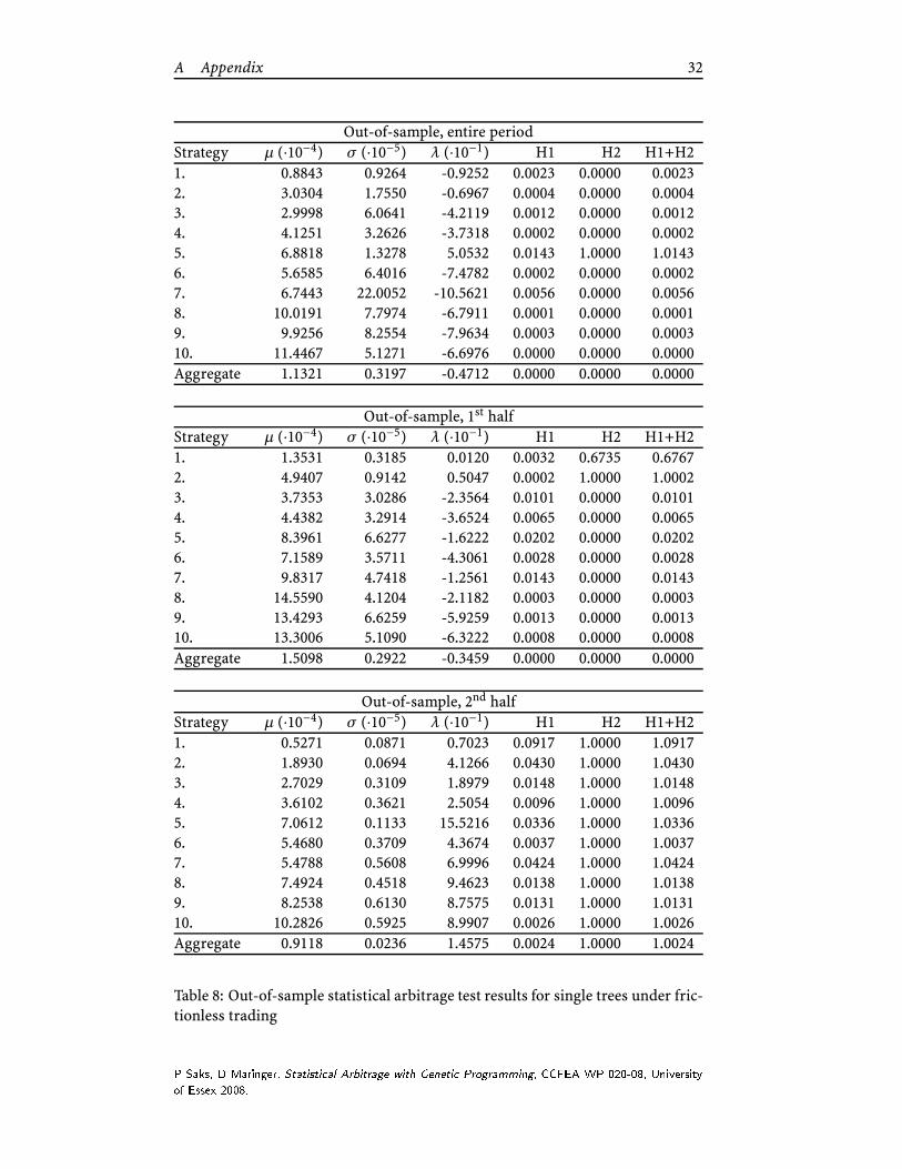
A Appendix 32

Out-of-sample, entire period

Strategy µ (·10−4) σ (·10−5) λ (·10−1) H1 H2 H1+H2

1. 0.8843 0.9264 -0.9252 0.0023 0.0000 0.0023

2. 3.0304 1.7550 -0.6967 0.0004 0.0000 0.0004

3. 2.9998 6.0641 -4.2119 0.0012 0.0000 0.0012

4. 4.1251 3.2626 -3.7318 0.0002 0.0000 0.0002

5. 6.8818 1.3278 5.0532 0.0143 1.0000 1.0143

6. 5.6585 6.4016 -7.4782 0.0002 0.0000 0.0002

7. 6.7443 22.0052 -10.5621 0.0056 0.0000 0.0056

8. 10.0191 7.7974 -6.7911 0.0001 0.0000 0.0001

9. 9.9256 8.2554 -7.9634 0.0003 0.0000 0.0003

10. 11.4467 5.1271 -6.6976 0.0000 0.0000 0.0000

Aggregate 1.1321 0.3197 -0.4712 0.0000 0.0000 0.0000

Out-of-sample, 1st half


1. 1.3531 0.3185 0.0120 0.0032 0.6735 0.6767

2. 4.9407 0.9142 0.5047 0.0002 1.0000 1.0002

3. 3.7353 3.0286 -2.3564 0.0101 0.0000 0.0101

4. 4.4382 3.2914 -3.6524 0.0065 0.0000 0.0065

5. 8.3961 6.6277 -1.6222 0.0202 0.0000 0.0202

6. 7.1589 3.5711 -4.3061 0.0028 0.0000 0.0028

7. 9.8317 4.7418 -1.2561 0.0143 0.0000 0.0143

8. 14.5590 4.1204 -2.1182 0.0003 0.0000 0.0003

9. 13.4293 6.6259 -5.9259 0.0013 0.0000 0.0013

10. 13.3006 5.1090 -6.3222 0.0008 0.0000 0.0008

Aggregate 1.5098 0.2922 -0.3459 0.0000 0.0000 0.0000

Out-of-sample, 2nd half


1. 0.5271 0.0871 0.7023 0.0917 1.0000 1.0917

2. 1.8930 0.0694 4.1266 0.0430 1.0000 1.0430

3. 2.7029 0.3109 1.8979 0.0148 1.0000 1.0148

4. 3.6102 0.3621 2.5054 0.0096 1.0000 1.0096

5. 7.0612 0.1133 15.5216 0.0336 1.0000 1.0336

6. 5.4680 0.3709 4.3674 0.0037 1.0000 1.0037

7. 5.4788 0.5608 6.9996 0.0424 1.0000 1.0424

8. 7.4924 0.4518 9.4623 0.0138 1.0000 1.0138

9. 8.2538 0.6130 8.7575 0.0131 1.0000 1.0131

10. 10.2826 0.5925 8.9907 0.0026 1.0000 1.0026

Aggregate 0.9118 0.0236 1.4575 0.0024 1.0000 1.0024

Table 8: Out-of-sample statistical arbitrage test results for single trees under fric-

tionless tradingP Saks, D Maringer, Statisti al Arbitrage with Geneti Programming, CCFEA WP 020-08, Universityof Essex 2008.

A Appendix 33



1. 0.4270 0.9883 -0.9490 0.0890 0.0000 0.0890

2. 2.3767 0.8413 -1.1663 0.0000 0.0000 0.0000

3. 2.0884 8.6617 -3.0194 0.0898 0.0000 0.0898

4. 3.8508 2.5737 -2.3889 0.0016 0.0000 0.0016

5. 5.9892 5.6713 -4.7637 0.0002 0.0000 0.0002

6. 6.3149 4.1970 -5.6355 0.0000 0.0000 0.0000

7. 6.1353 3.4051 -4.9456 0.0005 0.0000 0.0005

8. 9.3698 11.0971 -8.2853 0.0005 0.0000 0.0005

9. 4.9583 5.1035 -7.2780 0.0191 0.0000 0.0191

10. 11.3825 36.1136 -13.8394 0.0052 0.0000 0.0052

Aggregate 0.9256 0.4083 -0.9219 0.0000 0.0000 0.0000



1. 0.7461 0.4129 -0.1682 0.0698 0.0000 0.0698

2. 2.9312 1.0145 -1.4424 0.0001 0.0000 0.0001

3. 3.0065 0.5772 3.8512 0.1135 1.0000 1.1135

4. 5.5651 1.7100 -0.8123 0.0028 0.0000 0.0028

5. 8.2239 3.1102 -2.0118 0.0011 0.0000 0.0011

6. 9.0387 3.1844 -4.0858 0.0001 0.0000 0.0001

7. 8.3983 3.5165 -4.9763 0.0013 0.0000 0.0013

8. 12.0766 6.0538 -3.9256 0.0034 0.0000 0.0034

9. 10.1617 3.2130 -3.4285 0.0031 0.0000 0.0031

10. 20.5271 3.8271 5.1127 0.0027 1.0000 1.0027

Aggregate 1.3707 0.1409 0.0069 0.0000 0.5978 0.5978



1. 0.1538 0.0577 1.0521 0.3495 1.0000 1.3495

2. 1.9715 0.1844 1.0428 0.0035 1.0000 1.0035

3. 1.5603 0.4178 3.1583 0.1993 1.0000 1.1993

4. 2.4974 0.1180 6.6822 0.0628 1.0000 1.0628

5. 4.6692 0.3059 5.6054 0.0143 1.0000 1.0143

6. 3.7745 0.4314 4.0292 0.0376 1.0000 1.0376

7. 4.5021 0.4896 4.8961 0.0351 1.0000 1.0351

8. 5.8471 0.8538 6.0689 0.0532 1.0000 1.0532

9. 0.9981 0.5332 7.1093 0.3740 1.0000 1.3740

10. 5.8397 4.2910 -0.6923 0.1430 0.0042 0.1471

Aggregate 0.5960 0.0299 0.9108 0.0122 1.0000 1.0122

Table 9: Out-of-sample statistical arbitrage test results for dual trees under fric-

tionless tradingP Saks, D Maringer, Statisti al Arbitrage with Geneti Programming, CCFEA WP 020-08, Universityof Essex 2008.

A Appendix 34



1. 0.7090 3.8864 -1.4343 0.0556 0.0000 0.0556

2. 0.8319 5.5430 -2.4060 0.1738 0.0000 0.1738

3. -0.0932 23.0714 -4.8673 0.5226 0.0000 0.5226

4. 0.8296 4.5428 -3.1347 0.2932 0.0000 0.2932

5. 5.5094 2.3301 0.4183 0.0067 1.0000 1.0067

6. 3.5796 3.2687 -4.3740 0.0151 0.0000 0.0151

7. 4.3059 19.4080 -9.8599 0.0542 0.0000 0.0542

8. 5.2725 4.6709 0.2396 0.0851 0.9661 1.0512

9. 5.3695 4.9030 -6.5609 0.0151 0.0000 0.0151

10. 4.3570 22.1748 -11.1114 0.1513 0.0000 0.1513

Aggregate 0.6456 0.6537 -0.6220 0.0233 0.0000 0.0233



1. 1.4027 1.5993 -0.6343 0.0292 0.0000 0.0292

2. 2.5672 3.7179 -1.6253 0.0361 0.0000 0.0361

3. 1.1144 11.7142 -2.9947 0.3431 0.0000 0.3431

4. 0.9082 3.0801 -1.5716 0.3523 0.0000 0.3523

5. 9.6970 2.0578 1.3027 0.0016 1.0000 1.0016

6. 6.1911 3.7696 -4.9463 0.0063 0.0000 0.0063

7. 8.3920 2.9048 1.4888 0.0306 1.0000 1.0306

8. 8.2825 15.5883 -7.4196 0.0639 0.0000 0.0639

9. 9.2866 5.6544 -7.4195 0.0063 0.0000 0.0063

10. 5.8946 16.6138 -8.1364 0.1912 0.0000 0.1912

Aggregate 1.1082 0.6270 -0.5279 0.0129 0.0000 0.0129



1. 0.4878 0.1051 1.0554 0.1818 1.0000 1.1818

2. 0.1644 0.1533 2.6634 0.4395 1.0000 1.4395

3. -0.5132 0.2623 4.5488 0.6053 1.0000 1.6053

4. 1.7130 0.2092 5.6897 0.1814 1.0000 1.1814

5. 3.4272 0.1224 11.6530 0.1006 1.0000 1.1006

6. 1.7482 0.3956 4.8485 0.2142 1.0000 1.2142

7. 2.8709 0.6345 6.4806 0.1874 1.0000 1.1874

8. 5.4380 0.1808 20.3875 0.1202 1.0000 1.1202

9. 2.6223 0.5934 7.2727 0.2142 1.0000 1.2142

10. 5.4774 0.8301 12.1285 0.1479 1.0000 1.1479

Aggregate 0.4813 0.0332 1.5544 0.1175 1.0000 1.1175

Table 10: Out-of-sample statistical arbitrage test results for single trees under 1bp

market impactP Saks, D Maringer, Statisti al Arbitrage with Geneti Programming, CCFEA WP 020-08, Universityof Essex 2008.

A Appendix 35



1. 0.5616 1.3266 -1.3337 0.0225 0.0000 0.0225

2. 0.4357 2.1637 -2.3541 0.2206 0.0000 0.2206

3. 2.4700 5.9105 -2.6596 0.0388 0.0000 0.0388

4. 1.6000 3.0816 -4.1689 0.0639 0.0000 0.0639

5. 1.5022 2.9575 -2.9591 0.1703 0.0000 0.1703

6. 0.4801 2.7877 -2.4133 0.4009 0.0000 0.4009

7. 0.8946 1.5847 -0.5873 0.3227 0.0000 0.3227

8. 9.5990 10.3110 -10.3717 0.0000 0.0000 0.0000

9. 5.5076 6.5143 -9.0015 0.0098 0.0000 0.0098

10. 8.4098 14.2737 -14.8195 0.0007 0.0000 0.0007

Aggregate 0.5510 0.4109 -1.0776 0.0017 0.0000 0.0017



1. 0.8301 0.7644 -0.8357 0.0333 0.0000 0.0333

2. 1.1584 0.7101 -0.4012 0.1038 0.0000 0.1038

3. 3.7076 9.2456 -3.7302 0.0386 0.0000 0.0386

4. 2.9040 2.7992 -3.8099 0.0356 0.0000 0.0356

5. 4.8148 2.5767 -2.1679 0.0221 0.0000 0.0221

6. 0.2698 2.1389 -0.8768 0.4624 0.0000 0.4624

7. 0.4799 1.5110 -0.0939 0.4325 0.3113 0.7438

8. 10.9036 6.6737 -7.1572 0.0014 0.0000 0.0014

9. 7.3459 3.4537 -3.7681 0.0252 0.0000 0.0252

10. 9.8926 5.8844 -7.1353 0.0106 0.0000 0.0106

Aggregate 0.7882 0.2712 -0.6919 0.0040 0.0000 0.0040



1. 0.3994 0.0765 0.6293 0.1310 1.0000 1.1310

2. 0.3352 0.0632 2.6392 0.3139 1.0000 1.3139

3. 0.8956 0.3228 3.7711 0.3125 1.0000 1.3125

4. 0.6556 0.5499 0.5441 0.3213 1.0000 1.3213

5. -0.8630 0.1888 7.2044 0.6653 1.0000 1.6653

6. 0.7175 0.9314 2.2604 0.3914 1.0000 1.3914

7. 1.1606 0.5307 5.3785 0.3332 1.0000 1.3332

8. 7.7866 0.4188 7.6383 0.0032 1.0000 1.0032

9. 3.8859 0.2989 10.6625 0.0934 1.0000 1.0934

10. 7.6731 1.1616 1.8053 0.0108 1.0000 1.0108

Aggregate 0.3783 0.0280 0.8117 0.0590 1.0000 1.0590

Table 11: Out-of-sample statistical arbitrage test results for dual trees under 1bp

market impactP Saks, D Maringer, Statisti al Arbitrage with Geneti Programming, CCFEA WP 020-08, Universityof Essex 2008.

Documents

WP020-08 Finance and - BRACIL for Computational Finance and Economic Agents Working Paper Series WP020-08 Philip Saks Dietmar Maringer Statistical Arbitrage with ... Statistical Arbitrage