1126 E. 59th St, Chicago, IL 60637 Main: 773.702.5599

bfi.uchicago.edu

WORKING PAPER

The Case of Brazil Márcio Garcia, João Ayres, Diogo Guillén, and Patrick KehoeAUGUST 2018

The Fiscal and Monetary History of Brazil: 1960–2016∗  

Marcio Garcia†  

PUC-Rio, CNPq and FAPERJ

Joao Ayres Inter-American Development Bank

Diogo Guillen Itau-Unibanco Asset Management

Patrick Kehoe Stanford University, Federal Reserve Bank of Minneapolis, and University College London

July 20, 2018

Abstract

Brazil had a long period of high inflation. It peaked around 100% per year in 1964, and accelerated again in the 1970s, reaching levels above 100% on average between 1980 and 1994. This last period coincided with severe balance of payments problems and economic stagnation that followed the external debt crisis in the early 1980s. We show that the high-inflation period (1960-1994) was characterized by a combination of deficits, passive monetary policy, and constraints to debt financing. The transition to the low-inflation period (1995-2016) was characterized by improvements in all those instances, but it did not lead to significant improvements in economic growth. In addition, we document a strong correlation between inflation rates and seigniorage revenues, but observing that the underlying inflation rates are too high for the modest levels of seigniorage revenues. Finally, we discuss the role of monetary passiveness and indexation in accounting for the unique features of the inflation dynamics in Brazil in comparison to the other Latin American countries.

∗We would also like to thank Marcelo Abreu, Persio Arida, Edmar Bacha, Marco Basseto, Tiago Berriel, Afonso Bevilaqua, Amaury Bier, Claudio Considera, Gustavo Franco, Fabio Giambiagi, Clau- dio Jaloretto, Eduardo Loyo, Timothy Kehoe, Randy Kroszner, Pedro Malan, Rodolfo Manuelli, Juan Pablo Nicolini, Affonso Pastore, Murilo Portugal, Thomas Sargent, Rogerio Werneck, and participants of the workshops on The Monetary and Fiscal History of Latin America held in Chicago, Buenos Aires (LACAE-LAMES meetings), and Rio de Janeiro (hosted by PUC-Rio). This project has been coordinated by Marcio Garcia. †The order of authors was selected randomly.

1   Introduction

This Chapter presents the monetary and fiscal history of Brazil between 1960 and 2016, with emphasis on the hyperinflation episodes. It describes the evolution of the Brazilian monetary and fiscal policy institutions and how they relate to episodes of macroeconomic instability and growth experience, focusing on the high-inflation period (pre–1994) and two stabilization plans: the Government Economic Action Plan (PAEG) and the Real Plan. The PAEG, in 1964, stabilized an inflation of around 100% per year, whereas the Real Plan, in 1994, stabilized an inflation of around 80% per month after six failed attempts in over a decade. The analysis follows the conceptual framework in Chapter 2, by focusing on the government budget constraint.

A summary of the period is illustrated in Figure 1, in which we show the evolution of real GDP per capita, inflation, and government deficit for the 1960–2016 period. Three subperiods are identified: (1) 1960–1980, fast economic growth with high inflation; (2) 1981–1994, slow growth with hyperinflation; and (3) 1995–2016, moderate growth with low inflation. The average deficit is similar across subperiods, being roughly the same in the earliest two subperiods and lower in the most recent one.1 One must bear in mind that fiscal statistics for earlier periods before 1997 are very flawed. For example, the deficit series in Figure 1c does not include investment by state-owned enterprises (SOEs) before 1985, and in the next sections we show that it represented an important source of government expenses in the earliest subperiods.2 The 1981–1994 subperiod stands out not only by its poor growth performance and hyperinflation, but also by severe balance of payments problems, a common feature among highly indebted Latin American countries affected by the increase in international interest rates and the slowdown in international economic growth.

When relating the episodes of macroeconomic instability to the government fiscal and monetary policies, we observe the following: (a) both stabilization plans, PAEG in 1964 and Real Plan in 1994, included measures to improve fiscal balances (although in the case of the Real Plan they took longer to be consolidated) and were followed by increased access to debt financing; (b) the government policy to increase public investment in the wake of the first oil shock in 1973 explains the rapid increase in external debt that preceded the external debt crisis of 1983; and (c) the high-inflation periods (pre-1994) were characterized by the combination of fiscal deficits, passive monetary policy, and constraints to debt financing, while the transition to the low-inflation period (1995- 2016) was associated with improvements in government fiscal balances, higher de facto independence of the monetary authority (Brazil still lacks a formally independent Central

1See Chapter 2 for the definition of deficit we use. It is the primary deficit over GDP plus real interest expenditures on debt discounting for real GDP growth.

2We refer the reader to the Data Appendix for a detailed description of the data and methodology.

Bank), as well as much larger access to debt financing. In comparison to other Latin American countries, the following two characteristics

make the Brazilian experience rather unique: a long period of high inflation, with annual inflation rates, on average, above 100% between 1980 and 1994, and modest levels of deficits for very high underlying inflation rates. We discuss two features that may explain these unique characteristics of the Brazilian hyperinflation: first, a poor institutional framework in which other public entities besides the monetary authority had indirect control over money issuance (we discuss that in Section 4.1); second, the combination of a high degree of indexation in the economy to past inflation with a passive monetary policy.3 Together, both features have created what has been called inflation inertia, which could explain why the Brazilian hyperinflation was a much more protracted process than elsewhere, and gave many the illusion that it could be cured without major improvements in the fiscal stance. We discuss this issue in Section 4.2 and in our final remarks.

This study is organized as follows: in Section 2, we present a summary of the government budget constraint; in Section 3, we provide a historical description of each of the subperiods 1960–1980, 1981–1994, and 1995-2016; in Section 4 we discuss the evolution of the institutional framework involving both fiscal and monetary authorities and the genesis of inflation inertia; in Section 5, we present our final remarks and conclusion.

2   The government budget constraint

We are interested in analyzing the evolution of the government budget constraint for Brazil from 1960–2016. Our attempt is to match stocks (debt figures) with flows (fiscal deficits), duly accounting for valuation effects. 4 Table 1 presents a summary of the results. 5 In order to finance interest payments and primary deficits, the government can either issue domestic and external debt, or issue money and receive seigniorage revenues. Transfers account for the residual.6

We divide the 1960–1980 subperiod into three parts: 1960–1964, 1965–1972, and 1973–1980. In 1960–1964, markets for government debt securities were still underdeveloped, and the government faced restrictions on both domestic and external debt financing. Interest payments were low, but primary deficits were on the rise, and

3Most prices, wages, taxes, and the exchange rate were indexed to past inflation, as well as asset prices. 4Mainly the effect of devaluations on foreign-currency denominated debt. 5Table 1 is computed using the general price index from Getulio Vargas Foundation, IGP-DI, which better approximates the GDP deflator. This price index is very sensitive to variations in the exchange rate, so we also report the results using the consumer price index from FIPE, instead. See Table 4 in the Data Appendix. 6Note that transfers in 1995–2016 is zero, and that is due to the methodology used by the Central Bank of Brazil when estimating the primary deficit. See Data Appendix.

had to be financed with seigniorage revenues. In 1964–1967 PAEG, the stabilization plan, implemented both fiscal and financial reforms, which reduced primary deficits and allowed the government to issue domestic debt securities. That accounts for the increase in domestic debt financing and reduction in seigniorage revenues that we observe in the 1965–1972 period. In the 1973–1980 period, on the other hand, we observe a rise in both debt financing in external markets and seigniorage revenues, which were associated with higher interest payments on external debt and a significant rise in transfers, the residual. 5 Fortunately, in this case, we can explain most of these transfers. In the wake of the first oil crisis, the government implemented policies that aimed at boosting investment through external borrowing, and that was done mainly through SOEs. The debt series that was used to compute the government budget constraint includes SOEs, but the primary deficit series does not. The increase in investment by SOEs accounts for a large fraction of the increase in transfers (see Table 2).6 Therefore, we think that deficits at the time are better represented by adding the transfers to the primary deficits reported.7 In 1981–1994, debt financing in external markets decreased sharply and interest payments on external debt increased as a reflection of the debt crisis that followed the hike in international interest rates. In that period, debt financing in domestic markets and seigniorage revenues were used to finance the payments of both principal and interests of the external debt as well as the primary deficits. In the most recent period, 1995–2016, we observe an increase in primary surpluses and a decrease in seigniorage revenues, with domestic debt replacing the external debt. As we will discuss, this pattern reflects changes in both monetary and fiscal policy institutions, with higher de facto independence of the Central Bank and higher control over the government budget.

In the next sections we provide a detailed historical background that describes the fiscal and monetary policies adopted in the 1960–2016 period that accounts for the evolution of the government budget constraint. But before, we discuss a few features of the Brazilian data regarding the primary deficits.

3   Historical description 3.1   1960–1980: fast growth with macroeconomic instability

Brazil went through important transformations during the first subperiod of our analysis. It moved from being a rural society, in which 55% of the population lived in rural areas, to an urban society, with 68% of the population living in cities. Its production

5Interest payments might be negative because we are discounting for growth rates in real GDP and for the monetary correction of the debt.

6According to Werneck (2014), the average capital expenditures of SOEs for the 1973–1980 period was 7.4% of GDP. According to IBGE - Estatısticas do Seculo XX, in Table 2, it was 4.7%. Both are in the ballpark of our residual. 7By doing so, we approximate what Central Bank of Brazil has done in its fiscal statistics starting in 1985. See Data Appendix.

structure shifted toward the manufacturing sector, which increased its participation in GDP from 32% to 41%, while the agricultural sector saw its participation reduced from 18% to 10%.8 It was a period of fast economic growth, with real GDP per capita increasing 4.6% per year on average. However, it was also a period of macroeconomic instability, with a deep recession in the early 1960s, increasing external indebtedness following the first oil crisis in 1973, and nominal instability. Inflation rates rose in the beginning and reached levels around 100% in 1964, when PAEG was implemented after a military coup. Inflation rates fell significantly, but started to accelerate again around the first oil crisis, in 1973, returning to three-digit levels in 1980.9

To understand the fiscal and monetary policy institutions that were in place during those years, one should note that it was a period of heated debate regarding the role of the state in promoting economic development, in which the government undertook major national development plans, such as the Targets Plan in 1956–1961, the National Development Plan I in 1972–1974, and the National Development Plan II in 1975–1979. That process also led to a surge in the number of public banks, with nine of twenty-six states creating their own banks between 1960 and 1964, and to the creation of some of the largest Brazilian SOEs, such as Eletrobras in 1962 and Telebras in 1972.10 As we discuss below, they would all play an important role in explaining the dynamics of the government budget constraint in Brazil.

3.1.1 1960–1964

Before 1964, the separation between monetary and fiscal policy institutions in Brazil

was almost nonexistent, in the sense that the government treasury had total control over money issuance. That was done through the Bank of Brazil (BB), which had the monopoly over money issuance and operated in many instances as the bank of the government, a commercial bank, and a development bank. Technically, the Super- intendency of Money and Credit (SUMOC) was the monetary authority, but its council was mainly composed of BB employees. At the time, the main monetary policy instruments that SUMOC used were control over the monetary base expansion, subsidized credit to the industrial and agricultural sectors, and interventions in the foreign exchange market. Some of those interventions aimed to protect the local industry by imposing restrictions on imports of products that were also produced locally, that is, they were used to implement import-substitution policies.11 There

8Data from the Brazilian Institute of Geography and Statistics (IBGE). 9For thorough analyses of that period, we refer to Orenstein and Sochaczewski (2014), Mesquita

(2014), Resende (2014), Lago (2014), and Carneiro (2014). 10The other well-known Brazilian SOEs Companhia Siderurgica Nacional (CSN), Companhia Vale do

Rio Doce, and Petrobras had been created in 1941, 1942, and 1953, respectively. 11That was done through both quantity (restricted access to foreign currency) and price restrictions.

was no centralized market in which one could trade government debt securities in Brazil. Debt contracts were very heterogeneous and faced legal limits on the nominal interest rates that could be charged (12% per year).12 With rising inflation, that led to a decrease in the stock of domestic debt before 1964 (Figure 2), while seigniorage revenues became the main source of funds for the government to cover its fiscal deficits, as Table 1 shows. Access to external debt was restricted in that period. Brazil had a balance of payments crisis in 1952, and faced balance of payments problems again in the late 1950s.13

On the fiscal side, Brazil already had a diverse set of tax instruments, such as income, import, and consumption taxes. They were cumulative instead of value-added taxes, and amounted to around 15% of GDP (Figure 3). There were no fiscal rules such as limits to fiscal deficits, and the government could adopt expansionary policies without explicitly indicating how to finance them.

In 1956–1961, President Juscelino Kubitschek launched the first major national development plan, the Targets Plan, which had ambitious goals to create the necessary infrastructure to facilitate the industrialization process in Brazil. The transportation and energy sectors were the main targets, and the country observed a rapid expansion of its highway and electric energy systems. That plan also became famous for the creation of the new capital city, Brasilia. Besides relying on government funds, that plan also counted with large foreign direct investment, especially in the automotive industry. During its implementation, Brazil experienced high growth rates in real GDP per capita, but entered a recession in the following years (1962 and 1963), accompanied by rising fiscal deficits and inflation. That crisis was followed by a military coup in 1964, and by the implementation of an economic stabilization program in 1964–1967, PAEG, that aimed to stop the inflationary process and resume growth through fiscal and financial reforms.14

PAEG was launched in November 1964. At that time, there was a clear relationship between inflation and the expansion of the monetary base (Figure 4), so the government understood that it should find alternative ways to finance its expenditures and investment projects other than through seigniorage revenues. The government tackled that problem on two fronts: a fiscal reform to decrease government deficits and a financial reform to create other financing options. On the fiscal side, the government increased its tax revenues to around 23% of GDP (Figure 3) and managed to reduce its fiscal deficits, as illustrated in Table 1 subperiod 1965–1972. That was achieved through the creation of new taxes, increases in existing tax rates, and modernization of the tax system with the introduction of a value-added tax. On the financial side, the main changes were the introduction of monetary correction (indexation) to circumvent the legal limits on nominal interest rates, the creation of the Central Bank of Brazil (CBB), and the adoption

12See Silva (2009) and Pedras (2009) for the history of the Brazilian government debt. 13In the late 1950s, Brazil started negotiations with the International Monetary Fund (IMF), but the

negotiations were suspended as Brazil did not accept its conditions. 14The military dictatorship would last until 1985.

of a banking system based on a clear-cut separation among commercial banks and nonbank institutions. These changes would have important implications for the inflationary process in Brazil.

Regarding CBB, it is important to mention that it was not created as an independent institution. The SUMOC’s council was restructured to form the National Monetary Council (CMN), which had regulatory powers over CBB and operates until today. The relationship between CBB and BB also deserves special attention. Many of the government policies, such as subsidized credit, were initially conducted by BB and they remained so after CBB was created. In order to facilitate the interaction between both institutions, the government created the Conta Movimento, which was a BB account that would show up in CBB’s balance sheet as an asset and whose balance should average zero. But in practice, that ended up providing BB with the control over money issuance, since it could withdraw funds automatically from that account, and that would be automatically matched by an expansion of the monetary base in CBB’s balance sheet.15 Section 4 discusses these issues in greater detail.

With respect to the monetary correction, the existence of indexed public debt held by private savers on a voluntary basis defined the bedrock for the development of financial markets in Brazil in the following years.

3.1.2 1965–1972

Between 1966 and at least 1971, the demand for public debt was growing faster ahead

of the government’s financial needs. The federal government’s overfinancing led to the institutionalization of mechanisms that increased the spending capacity of local governments, a phenomenon that would eventually pose great fiscal challenges taking years to be reverted.

The 1968–1973 period became known as the years of “economic miracle” in Brazil, with annual GDP growth rates in excess of 10%. That led to the optimistic view that the Brazilian state had created a wholesome mechanism to capture private savings and channel them to public investment. The idea of complementarity between public and private investments reinforced the view that public debt was a key element in channeling funds for more investment, either public or private. During those years the government implemented the National Development Plan I (1972–1974), focused on improving the country’s infrastructure. It included large projects such as the Itaipu Dam, Trans-Amazonian Highway, and Rio-Niteroi Bridge. The country also experienced higher investment by SOEs and increasing supply of credit by public banks, such as BB and the National Bank for Economic Development (BNDE).16

15The original deficit series does not include the operations of BB, but since Conta Movimento was used to make transfers from CBB to BB, we added its variation to the deficit series. See Data Appendix. 16BNDE was established in 1952, and later became the National Bank for Economic and Social De-

3.1.3 1973–1980

When the first oil crisis in 1973 challenged the feasibility of the high-growth path, the Brazilian government kept its long-run strategy in the President General Geisel years (1974-79) to grow its way out of the first oil crisis, even if it had to rely on further deepening of public indebtedness supported by the growth of external liquidity. That explains the rapid increase in external debt in Figure 5 and accounts for the rise in external debt financing in the 1973–1980 period in Table 1. One of its goals was to reduce the country’s dependence on oil imports, using the SOEs as its main implementation vehicle. As part of this strategy, the government implemented the National Development Plan II in 1975–1979, which focused on the manufacturing, energy, transportation, and communication sectors (see Table 2). The external debt series does not allow us to distinguish SOEs from the rest of the public sector before 1981, but in that year external debt of SOEs represented 72% of the total, which indicates that they accounted for a large fraction of the increase in external debt after 1973 (Figure 6a). The same holds for the domestic debt, although in that case the concentration of SOEs was less pronounced. They accounted for 45% of the total domestic debt in 1981, while 33% was from states and municipalities, and 22% from the federal government (Figure 6b).

That period was characterized by the poor management of the government budget, so it is important to take into account the off-budget transactions when analyzing the dynamics of the government budget constraint during those years.17 The government operated two budgets, one that was discussed in the Congress, and the monetary budget, controlled by the CMN (see Section 4). In addition, the government did not have control over the budget of its SOEs. Given the deterioration of their accounts and trying to control that process, the government created the Secretary of Coordination and Governance of State-Owned Enterprises (SEST) in 1979. Figure 7 shows the deficit series including transfers, and we observe that government deficits increased significantly during that period. Besides the increasing indebtedness, the country also observed an increase in subsidies and subsidized credit provided by public banks to state and local authorities and to the private sector, reflected by the increase in transfers from CBB to BB through the Conta Movimento (Figure 8).

The strategy to sustain growth through external borrowing was successful in the first few years, as the accumulation of public debt was compatible with the maintenance of economic growth at high rates. Continuity of this process of growing indebtedness, however, relied on other factors: on the growth of private wealth, on the wealth holders’ confidence in the prospects of public sector ability to serve the debt, and on the use that

velopment (BNDES). See Costa Neto (2004) for the history of public banks in Brazil. 17The main off-budget transactions we identified were the operations of BB and SOEs. The former is

captured by the transfers made from CBB to BB through Conta Movimento, and we added its variation to the original deficit series. Those are the deficit series used to construct Table 1. The operations of SOEs are partially captured by the transfers before 1985, since they are included in the external debt series. See Data Appendix.

was ultimately being made of the savings captured by the government. In the second half of the decade, GDP growth declined sharply, inflation doubled, and there were increasing difficulties in controlling the growth of the public sector financial needs. Average maturity of federal government domestic debt securities reached its peak in 1975 (Figure 9), but the share of nominal bonds kept growing (Figure 10) until the end of the decade, as interest rates began to rise in 1976 following the abandonment of the interest rate ceilings, which had prevailed until September 1976.

The first year of President General Figueiredo’s term (1979) started with a reduction in the real value of public bond debt due to two effects: first, the decline in nominal interest rates promoted by Planning Minister Delfim Netto, the new economic czar, in an attempt to stimulate economic activity, which reduced the attractiveness of the debt;18 second, the increase in exchange rate uncertainty related to the second oil crisis. Figure 11 shows how interest rates were kept consistently below inflation rates between 1979 and 1981. Both factors reduced the attractiveness of the public debt in private portfolios. From 1971 onward, nominal Treasury Bills (LTNs) had been issued side-by-side with the old Indexed Treasury Bonds (ORTNs) as a result of the success of the reforms. In contrast with the ORTNs, which were held both by financial and nonfinancial institutions, LTNs were the typical assets used as reserves by financial institutions. They were auctioned at a discount only in large denominations, with maturity ranging from 30 to 720 days. CBB’s daily operations to regulate short-term liquidity via open market operations were collateralized by LTNs, while ORTNs were thought as adequate to provide steady finance for the structural fiscal deficit of the federal government. CBB’s portfolio, therefore, was concentrated by-and-large in LTNs.

The real value of indexed debt reached a plateau and stabilized in the middle of the decade, so that further finance for the public deficit came from the steady increase in the stock of LTNs between January 1975 and October 1978. The share of ORTNs held by the private sector declined by half at the end of the decade as the duration of the debt shrank in face of higher inflation and unstable interest rates. The average maturity of public debt fell from 1.42 to 1.16 years between 1977 and 1979 (Figure 9), when the widespread practice of repurchase agreements by CBB made it harder to ascertain the actual demand for longer-term debt.

The policies implemented by Delfim Netto, mainly low interest rates and change of wage indexation rules, from once to twice a year, had the effect of significantly increasing inflation, from around 50% in 1979 to over 100% in 1980, as argued in Simonsen (1983).

18Delfim Netto replaced Mario Henrique Simonsen in August 1979 as the de facto manager of the economy, less than six months into the new government of President General Figueiredo.

3.2   1980–1994: no growth with high macroeconomic instability

If the previous subperiod was characterized by the number of national development plans that were implemented, the subperiod 1980–1994 is famous for its number of stabilization plans, some of them indicated in Figure 12, and by severe balance of payments problems.19 In this section, we discuss Brazil’s balance of payments crisis and provide a description of its stabilization plans during the 1980s and early 1990s, focusing on their main points and reasons for their failures, and trying to find out the most important differences between them and the ultimately successful plan (Real).

Even though inflation was increasing to rates above 100% per year, in the first half of the 1980s there were larger concerns to reduce external imbalances than to reduce inflation. In 1981 and 1982, the main objective of Brazil’s macroeconomic policy was to reduce the need for foreign capital. Figure 13 shows the current account balance, trade balance, and net interest income, and we can observe the increasing cost of interest payments on external debt and the trade balance reversal (from deficit to surplus) in those years. There was a large devaluation of the real exchange rate (Figure 14), and real GDP per capita contracted sharply.20 In 1982, Brazil would enter a sequence of episodes in which it accumulated arrears on interest payments of its external debt, illustrated in Figure 15, that would only end in 1994.21 These facts account for the drop in external debt financing and rise in interest payments on external debt reported in Table 1, subperiod 1981–1994. During that period we also observed the nationalization of the external debt. Foreign debtors would pay CBB in domestic currency and CBB would not pay the external creditor. After a few years, CBB allowed external creditors to exchange their funds retained at CBB by domestic assets.22 Figure 16 shows that a large fraction of the external debt became concentrated in CBB’s balance sheet up to 1994.

While government’s attention was focused on the balance of payments crisis, inflation kept increasing. It was only in 1986 that the sequence of stabilization plans began. But before moving to the discussion about each stabilization plan in detail, it is important to put into perspective the cause of high inflation was at the time. The Cruzado Plan, as well as the Bresser and Summer plans, considered that inflation inertia due to the highly indexed economy was the essence of the inflationary process, and it should be the main focus of the stabilization plan. These plans had a “neutral shock” of freezing prices as one of their main characteristics. However, the staggering of wages and other prices under very high inflation was an extra obstacle to a heterodox plan. At the moment that a shock to stop inflation was introduced, agents with similar average real wages would have different real wages depending on when the

19For thorough analyses of that period, we refer to Carneiro and Modiano (2014), Modiano (2014), and Abreu and Werneck (2014).

20According to our definition of exchange rate, a real depreciation happens when its value increases. 21See Cerqueira (2003) for a description of the external debt negotiations during that period. 22See Cerqueira (2003).

last adjustment was set. Since inflation was supposed to decrease substantially after the plan, the differences in real wages at the moment of the plan would prompt losers to claim rights to be compensated, while the winners would not complain. If the losers were compensated, that would reignite the inflation spiral. To avoid that problem, a conversion table was always mandated at the beginning of each plan, aiming at keeping, in the new low inflationary environment, the same average real wage that had prevailed under the previous high inflationary period.23

As we will see, from the first to the last plan there was a decrease on the emphasis on the heterodox part of the plan, which comprised price freezes, and more emphasis on the orthodox part. Fiscal and monetary policies became a major component of the latter plans, while maintaining a device to synchronize the adjustment of nominal variables to avoid threatening the new low inflation level.

Cruzado Plan: In February 1986, the government implemented the Cruzado Plan. As it became standard in some Brazilian stabilization plans, the first rule was to change the currency, in that case from cruzeiro to cruzado, which meant cutting three zeros. Prices were frozen.24 Wages were converted into cruzados based on the average purchasing power of the last six months but could be readjusted every time inflation hit 20% or during the annual readjustment cycle. Moreover, unemployment benefits were introduced and the minimum wage was raised by 8% in real terms. The exchange rate regime also changed, with the domestic currency now pegged to the US dollar. The plan also extinguished monetary correction, and any indexation clauses for periods shorter than one year were forbidden.25 Fiscal and monetary policies were put under the discretion of the policymakers, but there was an important change, the end of the Conta Movimento between CBB and BB. As previously mentioned, the Conta Movimento worked as free money that BB would use whenever prompted to further extend financing to sectors or firms targeted by economic policy. In practice, however, that took place only after 1988, because another account between CBB and BB, Conta de Suprimentos Especiais, replaced Conta Movimento until its extinction in 1988 (see Section 4). Another important measure was the creation of the Department of the Treasury, which would take control over both the administration of the domestic public debt and the government budget.26

23The change of currency allowed for reductions of those wages that had been recently adjusted, in order to keep the same average real wage. Without the change of currency, the reduction in nominal wages would not be possible since nominal wage reductions are not allowed by Brazilian Law.

24Except for electricity, which had a 20% increase. 25For fixed-rate contracts, a schedule for interest rate conversion was set. It was assumed that all

nominal interest rates were based on the inflation expectation of 0.45% a day (210% a year), which had been the average daily inflation in 1985/86. The real rate was, then, the (new) nominal rate in the new currency (cruzado), since the new expected inflation (at least for the government) was zero. For the variable interest rate contracts, which prescribed a nominal rate equal to the sum of the monetary correction and a variable (real) interest rate, the new nominal rates in cruzados were set to be the ones above the monetary correction before the plan.

26Before that, CBB managed both the domestic and external public debt.

At first, the Cruzado Plan was very successful in reducing inflation. The average monthly inflation from March to July 1986 was 0.9% (IGP-DI). Moreover, the claim to freeze prices had a civic impact since the population felt that they were “auditing prices.” But that led to overheating. Sales increased 23% in the first six months of 1986 compared to the first six months of 1985. Real wages increased 14% from March to September of 1986 (Figure 17). One consistent story with such evidence is that even though prices were not allowed to change, the “equilibrium prices” were increasing, which was producing overheating since posted prices were too low. It is clear that there was political pressure to avoid a recession or bring inflation back to high levels. On the other hand, CBB tried to keep interest rates low to induce low expectations. In the end, the monetary base was increasing much faster than inflation itself (Figure 4a). Something needed to be done. Many products became scarce, but nobody wanted to bear the political burden of a recession.

In July 1986, the government introduced a timid fiscal package (Cruzadinho) involving compulsory loans on fuel, car purchases, and international airline tickets and foreign exchange sales for travel expenses. But in reality Cruzadinho had the opposite result from what policymakers expected. Expecting prices to defreeze, demand increased and the overheating problem became even more dramatic. Inflation remained low, but it was not really representative, because products were scarce. Due to the high demand, imports kept increasing while exports declined (Figure 18), thereby aggravating the trade deficit. A rumor of a large devaluation in the near future reinforced that pattern. This expectation lead to a postponement of exports and acceleration of imports, which augmented the balance of payments problems.27 Facing all these challenges, in November 1986, the government opted for a fiscal plan, Cruzado II, trying to increase revenues through the readjustment of some public prices and some indirect taxes, which led to a high inflationary shock. It was again an environment of high inflation (17% per month in January 1987). The external crisis was just getting worse. In February 1987 the government suspended the interest payments on the external debt (see Figure 15) for an indeterminate time). The idea was to stop the losses of international reserves and to start a new phase on the renegotiation of the debt with the support of the population.

Bresser Plan: In July 1987, the government implemented the Bresser Plan. It was presented as a hybrid plan, with fiscal and monetary policies as well as aspects to deal with inflation inertia. Just like the Cruzado Plan, prices were frozen. As usual, the moment in which the price freeze took place was important, because the relative prices would remain stuck and possibly off-equilibrium. In an attempt to get a better result than the Cruzado Plan on this aspect, after the price freeze there was an increase in the prices of public services and some administered prices to correct for misalignments in relative

27The government kept the minidevaluations based on an indicator of the ratio exchange rate /wage (crawling peg). However, this same indicator suggested that the exchange rate was appreciated.

prices. The extinction of the automatic trigger in wage resetting if inflation surpassed a 20% was also perceived as another improvement. The trigger was extinct, but the economic team created another kind of wage indexation, the URP (price reference unit). Every quarter, the government would specify the readjustment for the next three months based on the average inflation of the period. This would keep a monthly readjustment, but there would be a gap between the readjustment and current inflation. In contrast to the Cruzado Plan, monetary and fiscal policies were active. Real interest rates remained positive in the short term. In the fiscal policy arena, the government aimed to reduce the operational deficit from the expected 6.7% to 3.5% of GDP.28 The plan also kept the default on the external debt. Another interesting aspect of this plan is that it did not target zero inflation, it was meant to be just a deflationary shock.

The main purpose of Bresser-Pereira, the finance minister, was to have a fiscal reform to reduce inflation. However, it was not successful. In 1987, the operational deficit was 5.5%, much higher than the promised 3.5%. Different from the Cruzado Plan, which had popular support, the Bresser Plan lacked popular support and, in February 1988, there was some liberalization of prices, reducing the effectiveness of the price freezing. As a third pitfall of the economic plan, gross fixed capital formation fell.

Feijao-com-Arroz Policy: In January 1988, the government adopted an economic policy referred to as Feijao-com-Arroz Policy, which can be translated to English as black- beans-and-rice policy. Its name reflects the meaning of black beans and rice in the Brazilian culture. It is the dish that Brazilians eat every day. It is not considered to be very interesting, or very difficult, but it does the job of providing a healthy meal. After Minister Bresser left, Maılson da Nobrega, the second in command, took his position. Instead of freezing prices, Nobrega sought to merely to keep inflation at 15% per month. The deficit was expected to reach 7%-8% of GDP in 1988, and there was a temporary freeze of public sector wages to reduce it.

At first, this policy succeeded in avoiding an inflationary explosion and the fiscal stance improved. The default on external debt was suspended and the government started negotiations with external creditors. However, inflation started rising again and the target of 15% per month was not achieved in the second quarter of 1988.

In October 1988, a new Constitution was enacted. The Brazilian Constitution increased expenditures and increased the transfers from the central government to states without transferring the corresponding responsibilities. It induced an increase in the deficit of the central government. Just to put this into perspective, 92% of revenues were earmarked. Among other measures not usually object of constitutional law, the new Constitution reduced the standard

28At the time the government used the public sector borrowing requirement as a measure of the nominal deficit. However, nominal deficits were very high due to the monetary correction of the value of the debt. In order to overcome that, the operational deficit was adopted as the main deficit measure, which included only the nominal value of real interest payments. See Data Appendix.

weekly working time from 48 to 44 hours and increased the cost of overtime. Not only did the Constitution increase the fiscal expenditures and reduce the flexibility of expenditure switching between fiscal accounts, it also increased labor costs substantially. On the external side, it should be mentioned that 1988 was a good year for the trade balance and the current account.

Summer Plan: The government implemented the Summer Plan in January 1989. Again, it was a hybrid plan, but the debate on the need for changes in fiscal and monetary policies was increasing. Like the previous plans, there was a component of price freezing as well as the adoption of a nominal anchor. In that case, a fixed exchange rate (1 Cruzado Novo = 1,000 Cruzados = US$1) was implemented for indefinite time. Moreover, there was an attempt to end inflation indexation. On the fiscal and monetary side, the plan was to adopt a tight monetary policy and to fight inflation by controlling the public deficit. It intended to control expenditures and increase revenues through the privatization of public-owned assets and reduction in the wage bill of the public sector. Overall, the plan seemed to incorporate everything that lacked in the previous plans. Although it kept a heterodox flavor (that is, it had an income policy component), the plan was mostly an orthodox one aiming to reduce subsidies, close public firms, and fire excessive public employees, with a deindexation plan that was sort of a small default. However, the government did not have the political power to carry it through. Without the Congress, privatizations and other unpopular measures, such as the closing of public firms, were canceled. In the end, the reforms were not implemented. Moreover, the tight monetary policy put interest rates at high levels and increased the fiscal deficit of the government. With low credibility and a reform that did not go through, inflation came back and the Summer Plan also failed.

The 1980s ended with almost 100% of the federal bond debt being rolled over in the form of zero-duration bonds.29 This state of affairs reflected not only the extremely high uncertainty regarding inflation and interest rates, but also the fear of an explicit default of the debt by the incoming administration of President Fernando Collor de Mello. At the time, there was a widespread suspicion regarding the credit risk of the public securities, which were indeed validated by the new administration’s actions. Fernando Collor de Mello was elected president of Brazil after 29 years of indirect elections or nondemocratic ones. The very day he took office, he launched the Collor Plan.

Collor Plan I: In March 1990, the government launched the Collor Plan I. It recognized that a reduction in deficits was necessary to end the hyperinflation, and it implemented both temporary and permanent fiscal policies. Among the temporary measures were the establishment of a tax on financial intermediation and the suspension of tax incentives. But the permanent policies were more important. There was an effort to

29Zero-duration bonds are bonds that pay ex-post the accrual of daily overnight interest rates. Therefore, the price of these bonds are insensitive to interest rate changes. It was a way to separate

interest rate risk from maturity risk, thereby lengthening a bit the very short-term public debt.

reduce fiscal evasion (one of his trademarks during the presidential campaign) and to increase taxes. The other major components comprised privatizations and an administrative reform. On the monetary side, the plan attempted to reduce the money supply by confiscating funds in both transactions and savings accounts for a period of eighteen months. Those funds would be kept at CBB and invested in government bonds, and represented 80% of bank deposits and financial investments. Finally, prices and wages were also frozen.

Following its implementation, monetary aggregates reduced sharply, especially the higher ones (Figure 19). This reduction of liquidity, however, was not sufficient to control inflation. Regarding the fiscal reform, the threatening behavior of the government toward the public sector employees turned the reform very unpopular. There was a lot of resistance and, in the end, it could not reach everything it proposed. Some privatizations succeeded, but most of the fiscal reforms were short-lived.

Collor Plan II: In January 1991, the same government implemented the Collor Plan II. Just like the previous one, it planned to reduce government expenditures by firing civil servants and closing public services. It also proposed the privatization of SOEs. As usual, the plan had a price freezing aspect. Wages were converted by a twelve-month average, a new tablita was adopted based on the assumption that the inflation would fall to zero, and it put an end to indexation.30 Not entirely related to the fight against inflation, this plan had a motif that Brazil had to improve the quality of its products. In the words of the president, “Brazil was producing horse-drawn coaches instead of cars.” To achieve that, the government opened the Brazilian economy to foreign competition and privatized state-owned firms.

Following its implementation, the country experienced a recession. But it recovered afterward, and this is usually attributed to enhanced competition in the economy. Inflation rose again, but this plan left two important permanent changes. First, it opened up the Brazilian economy. The trade chain increased in 1990, reversing the previous trend. Second, productivity increased. In the beginning of 1992, when expectations of accelerated inflation did not materialize, the effects of recovered investors’ confidence started to appear in public debt markets. Those expectations had been based on the combination of price liberalization, corrections of public tariffs, and on the devaluation that followed the floating of the exchange rate in October 1991 in face of the strong monetization of the hijacked assets during Collor Plan I.31 The return of investors’

30Tablita was the name for the interest rate conversion table when the currency changed. 31The recovery of the stock of public debt in the portfolio of the private sector was a clear

demonstration that asset-holders were willing to return to business as usual in spite of the violence of repeated interventions, which had been made in the rules of indexation and liquidity of public securities in the previous twelve years. One should bear in mind that the majority of economic analysts at the time were forecasting that the government would never again be able to place new debt.

confidence is also confirmed by the recovery of foreign exchange reserves after 1992. Following the high political turbulence that characterized the months preceding the

impeachment of President Collor de Mello (October 2, 1992), the beginning of Itamar Franco’s presidency was marked by high uncertainty concerning economic policy. Proposals of another moratorium, and even repudiation of the public debt, were constantly in the press. It was only after the president nominated his fourth minister of finance in less than six months that the recovered confidence materialized in higher external reserves.

Real Plan: In June 1994, the government launched its last stabilization plan, the Real Plan, that would finally put an end to the hyperinflation. A new currency was created, the real, valued at 2750 cruzeiros reais. The plan that would eventually conquer Brazilian inflation did not have the blessing of the International Monetary Fund (IMF), an always troubled relationship in the previous decades. It had different concepts from the previous ones, aiming to reduce deficits, to modernize firms, and to reduce the distortions that arose from previous price freezes. The first stage of the Real Plan was defined by the fiscal element. Different from the previous plans that originally had the fiscal component but ended up unsuccessful in its implementation, the Real Plan had the fiscal component negotiated with the Congress. The Programa de Acao Imediata (Program for Immediate Action) was designed to focus on fiscal imbalances that would arise when the seigniorage revenues fell. A significant adjustment came in the beginning of 1994, with the Fundo Social de Emergencia (Emergency Social Fund), a way to suspend part of the earmarked revenues of states and municipalities. Despite its ambitious reform goals, the government ended up targeting what was available at that time to generate fiscal revenues, and it increased taxes of financial intermediaries. On the monetary side, a clearly stated intention to limit issuances of the new currency led to the adoption of a high interest rate policy and of high reserve requirement ratios (100% reserve requirement on new deposits after July 1st).

The Real Plan did not involve price freeze itself, but it was able to solve the problems of staggered wages and prices. Actually, this was considered the most controversial aspect of the plan, but probably the most ingenious and ultimately very successful. The creation of a new unit of account URV–Unidade Real de Valor (Unit of Real Value)–aimed at establishing a parallel unit of value to the cruzeiro real, the inflated currency. The idea was to make it temporary. Prices were quoted both in URVs and cruzeiros reais, but payments had to be made exclusively in cruzeiros reais. The way the URV worked was like a shadow currency that had its parity to cruzeiro real constantly adjusted, since it was one-to-one with the dollar. Therefore, a conversion rate of the URV/cruzeiro novo (the old currency) rate was set every day. With that system, the relative price problem was diminished. Many conversions were left to free negotiation between economic agents, with the government having more interference in oligopolized prices. Wages, for instance, were converted into URVs taking into account their real value in the last four months, as

this was the inherited indexation horizon. The objective was to get relative prices right. The URV was extinguished July 1, 1994, when it was converted to a new currency, real, with the parity being 1 dollar = 1 real = 1 URV.

3.3   1994–2016: moderate growth with higher stability

One of the conditions for the success of the Real Plan was the availability of foreign finance. From April 1993 to July 1997, foreign capital inflows resumed as Brazil’s relations with the international financial community were back to normal, putting an end to a long process of foreign debt rescheduling under the Brady scheme. The capital inflows were a main factor in the expansion of the interest-bearing public debt, as CBB conducted massive sterilized purchases of foreign exchange.32 The tightness of the monetary policy that followed the Real Plan still characterizes the monetary policy today. In fact, the Real Plan failed to achieve its monetary targets, but for a good reason: money demand vigorously expanded in face of low inflation. Not achieving its monetary targets had no effect, since monetary policy was very restrictive, judging by the high real interest rates. The Real Plan kept the process of opening the economy to foreign trade, enacted measures to support domestic industry modernization, and accelerated the privatization program. It should be stressed, however, that Collor II had all these objectives but in a more timid way. Even though it is always risky to discuss the success of a “contemporaneous” plan, it has been almost twenty-five years since its launch and inflation has been stable throughout most of this period. Many institutional reforms have been accomplished, like the introduction of a monetary policy committee, inflation targeting, and the Law of Fiscal Responsibility. On the fiscal side, sustainable primary surpluses were observed during the first decade of the twenty-first century. However, a major fiscal deterioration occurred from 2011 until 2016, creating an impending fiscal crisis. A broader fiscal reform is needed for the incoming president in 2019. Social security, for instance, remains to be overhauled. With the current rules, fiscal collapse is a certainty.

On the monetary side, the great switch was in 1999, when, after a speculative attack, the controlled exchange rate through a slow crawling peg was replaced by inflation targeting with a floating exchange rate. The switch was somewhat brisk, with several speculative attacks leading to eventual floating in early 1999, after the president achieved reelection promising to keep the exchange rate regime, and reneging on the promise very early in the new term. Even though inflation was high when the currency regime switched in 1999 (9%), it was nothing compared to the high inflationary period. An inflation targeting monetary regime has been working well for almost two decades.

32In 1993, so much capital was flowing into Brazil that the government implemented controls on capital inflows (Carvalho and Garcia, 2008).

We now turn to the discussion of two themes that were key to overcome the hyperinflation: institutions and inertia.

4   Institutions and inflation inertia 4.1   Weak institutions that provided indirect access to the

printing press

One of the most striking features of the Brazilian monetary and fiscal history is its long period of high inflation pre-1994, and Figure 4 shows that inflation rates were closely related to the growth rates of the monetary base and to seigniorage revenues. We argue that the high degree of passiveness in monetary policy during that period goes a long way in accounting for these facts. In this section, we present the history of the Central Bank of Brazil (CBB), from the discussions surrounding its creation up to the recent period in which it successfully implemented the inflation targeting regime. We also discuss how the government accessed seigniorage revenues and how CBB was used many times to perform operations that are not consistent with the notion of an autonomous monetary authority.

Before 1945, there was no clear separation between monetary and fiscal authorities, in the sense that the government treasury had total control over money issuance. That was done through the Bank of Brazil (BB), which had the monopoly over money issuance and operated in many instances as: the bank of the government, a commercial bank, and a development bank. The debate surrounding the establishment of CBB started before 1945, but it was only in that year when the first measures took place. The government created the Superintendency of Money and Credit (SUMOC), whose council would have regulatory powers over BB’s monetary affairs and should serve as a stepping stone towards the creation of the Central Bank. However, BB received the majority of seats in that council, which implies that there was no major improvement in the way monetary policy was conducted in practice. Therefore, instead of establishing a central bank directly, Brazil opted for a two-step approach, in which the first step, SUMOC, lasted twenty years. That process reflected a political impasse, with many political groups reluctant to loosen access to money issuance and subsidized credit.

In 1964, CBB was finally established. However, it was not created as an independent central bank. The SUMOC’s council was restructured to form the National Monetary Council (CMN), which had regulatory powers over CBB and operates until today. In the beginning, it had nine members: the finance minister, the president of BB, the president of BNDE, and other six members with fixed terms of six years each. Four of those six members would comprise the board of CBB, one as its governor. Although the fixed mandates provided some independence to CBB, it did not last for long. In 1967, during

the first transition of power within the military regime, the board of CBB was forced to resign, which included its governor, and the fixed terms were officially abolished later on. The evolution of the number of members in CMN and its composition provide an interesting perspective of the passiveness of monetary policy in Brazil, because, in practice, that council ended up operating a separate budget from the one approved in the Congress, usually referred to as the monetary budget. In the hyperinflation periods, the number of members in CMN increased to twenty-six, and they came from very different sectors of the government and society, including representatives of labor unions and business leaders. It was only in 1994 that the Real Plan reduced its number of members to the actual three (the president of CBB, the finance Minister, and the minister of planning), granting the board of CBB greater control over monetary policy.33 Figure 20 shows how the number of members in CMN changed over time. As remarked by Franco (2017), the correlation between inflation and the numbers of CMN members is remarkable.

Regarding CBB’s operations, Figure 21 shows the evolution of CBB’s balance sheet between 1965 and 2016, separating assets from liabilities. The complexity of its balance sheet during the high-inflation period shows that it was used many times to perform operations that are not standard to central banks, and most of the time that was done under the discretion of the government and not of the monetary authority itself. For example, upon its creation, the share of the monetary base in CBB’s liabilities was only 50%. The reason is that, instead of focusing exclusively on monetary policy, CBB also acted as a development bank. Some funds related to government economic policies, such as the provision of insurance to agriculture (PROAGRO) for example, were transferred to CBB.

Besides that, CBB became responsible for managing both the domestic and external public debt, which involved their issuance and payments of principal and interest. During the external debt crisis, for example, CBB was one of the main players involved in the negotiations, and it exchanged most of the external debt of domestic agents by domestic debt in local currency. That is, there was a nationalization of the external debt, in which CBB became the main responsible for it. That explains the rise in foreign currency obligations in CBB’s liabilities. That was also an important change implemented by the Real Plan, which transferred the administration of the external debt to the national treasury. At the time, the government clearly stated that it was done to avoid monetary pressure.

In 1986, the government created the Department of the Treasury (STN-Secretaria do Tesouro Nacional), which became responsible for managing the domestic debt. However, CBB was still authorized to purchase government debt securities directly from the treasury under special circumstances, such as in the case of failed auctions. That was forbidden in 1988, but evidence suggests that it kept doing so until the implementation of the Real Plan, which partially accounts for the concentration of federal government debt

securities in CBB’s balance sheet. If we analyze CBB’s operations during the high-inflation period, we do find evidence

that the government had access to and was using the seigniorage revenues. Up to 1988, that was done mainly through its operations with BB. As mentioned before, many of

33See Franco (2017) for a complete description of that process.

the government policies, such as subsidized credit, were initially conducted by BB and they remained being so after CBB was created. In order to facilitate the interaction between both institutions, the government created the Conta Movimento, which was a BB account that would show up in CBB’s balance sheet as a credit and whose balance should average zero. In practice, that provided BB with the control over money issuance, since it could withdraw funds automatically from that account, and that would be automatically matched with an expansion of the monetary base, of equal value, in CBB’s balance sheet. Not surprisingly, Figure 8 shows that the correlation between variations in that account’s balance over GDP and seigniorage was very high, and that a large part of seignorage was “spent” funding credit programs through BB. Since BB worked in large measure as the government’s banker (Pastore 2015), this should not be a surprise. Initially, CBB did not transfer its profits to the government treasury, so the use of Conta Movimento was a direct way in which the government could access the seigniorage revenues. Interestingly, when that account was frozen in 1986, the government started to use another similar account between BB and CBB, Conta de Suprimentos Especiais, until its extinction in 1988.34 When both accounts became unavailable, the government established the transfer of CBB profits to the treasury.35 In fact, after 1988, there were two ways in which the government could access seigniorage revenues: through the transfer of profits, and through the remuneration of its deposits at CBB. The New Constitution in 1988 established that the government could not have accounts with commercial banks, only

one account at CBB, the Conta Unica do Tesouro (Government Unique Account), which could be used for all its transactions. A particular feature of this account is that CBB became responsible for paying interests on its balance, which was based on the average remuneration of the government debt securities in its portfolio. Since deposits are usually not remunerated, those transfers can be interpreted as an anticipation of profits. Figure 22 shows the value of such transfers and how they match well with the series of seigniorage revenues. Therefore, the discussion above shows that the persistence and magnitude of the Brazilian inflation process is closely related to the persistence and magnitude of the degree of passiveness of its monetary policy. That changed significantly with the Real Plan.

4.2   Inflation indexation and passive monetary policy

In this subsection we outline the ingredients that created the so-called inflation inertia in Brazil, and how they interact. Basically, the main ingredients were mandatory

34Between 1965 and 1987, the average variation in the monetary base over GDP was 2.6 percent, while the average variation in BB accounts over GDP was 2.8%. Those figures show that seigniorage revenues were mostly used to finance BB operations. 35See Carvalho Jr. (2017) for a description of the evolution of the institutional framework regarding the relationship between CBB and the government treasury.

inflation indexation of prices, wages, taxes, and the exchange rate to past inflation, and a peculiar form of monetary passiveness.

Most inflationary processes show some degree of positive autocorrelation. We keep the term inertia to a special case of positive autocorrelation, when the inflation process exhibits a unit root (Pastore 2015, chapter 2; Cati, Garcia, and Perron 1999; Garcia 1997). This corresponds to the idea that any inflationary shock gets permanently incorporated into the inflation rate, not been dissipated over time.

The interaction between mandatory indexation to past inflation and monetary passiveness is what produced inflation inertia. The basic idea is that indexation to past inflation produces a continuous increase in nominal money demand. As the monopsonist in the money market, the Central Bank could, in theory, opt not to validate such an increase in money demand, by not increasing money supply, that is, by substantially increasing the real interest rate. However, this was not the monetary policy that was followed during the pre-Real Plan years. Monetary policy at the time was more akin to keeping the ex ante real interest rate at a low positive level. In terms of a simple Taylor rule, it would be as if the constant term were low, and the Taylor coefficient were near one. As Taylor (1993) has shown, analyzing more than one hundred years of monetary policy in the US, interest rate rules where the Taylor coefficient was near one, as the one followed during the 1960s and 1970s in the US (before Paul Volcker became Fed chairman), tend to generate high inflation. For Brazil before the Real Plan, the basic idea is that indexation by itself would increase the nominal demand of money, and that would be satisfied by the passive monetary policy, perpetuating inflation.

It was, therefore, the combination of indexation to past inflation and a passive monetary rule that created inflation inertia. In that environment, inflationary shocks, like the maxi-devaluations undertaken during external crises, permanently increased the inflation rate.

This may help explain why the Brazilian hyperinflation was a much more protracted process than elsewhere, and also gave many economists the illusion that it could be cured without major improvements in the fiscal stance. We discuss that in our final remarks.

5   Final remarks and conclusion

From the description of the plans, one sees that all of them were a convex combination of fiscal and monetary policies with some sort of policy to avoid the inertial effect. Moreover, there was an increase on the fiscal and monetary part across time, suggesting that the “orthodox” part was getting more importance. Looking from today’s (2018) perspective, one could say that even though the monetary policy seems to have been fixed, in 1995 with very high real interest rates coupled with a crawling peg and, since 1999 with inflation targeting, fiscal policy is still a major source of worries in

Brazil. Figure 3 shows that primary expenditures and revenues have been rising fast since the late 1980s, when Brazil returned to democracy.

This paper has so far presented a very interesting puzzle: why, unlike its six predecessors, did the 1994 Real Plan succeed in lowering inflation if it did not bring much fiscal improvement? The most likely explanations for this puzzle involve fiscal aspects, but also have to do with indexation, inflation inertia, and passiveness of monetary policy. We now turn briefly to those issues.

Inflation effects on fiscal (perfectly indexed) revenues and (not-so-well-indexed) outlays: Usually, the hyperinflation literature refers to the so-called Olivera-Tanzi effect. This is the effect that high inflation has on government revenues. Since usually government revenues are computed from nominal values, e.g., nominal income, and there is a lag until tax payment, the real value of taxes collected tend to fall with inflation. However, for the Brazilian case before the Real Plan, there are empirical indications (Bacha 2003) that the Olivera-Tanzi effect worked the other way around, for two reasons: first, fiscal revenues were very well indexed to inflation. Tax indexation was perfected to a point of almost keeping the real value of taxes collected immune to inflation. A daily index, the UFIR (Fiscal Reference Unit), was computed based on inflation. Taxes would be denominated in this indexed unit of account and translated to the nominal hyperinflated currency on the very day taxes were paid into the banking system. Second, fiscal expenditures were only imperfectly indexed to inflation. The fiscal budget was not so perfectly indexed as tax collection and always underestimated true inflation. Therefore, the real value of expenditures budget would invariably undershoot the originally budget real amount. The executive branch could, and indeed did, cut the real value of expenditures only by disbursing the originally planned nominal amounts with delay. Higher inflation would rapidly erode the real value of those expenditures. Of course, this had the collateral effect of creating large problems, since public hospitals would run out of money at the end of the year, several bridges or roads would stay unfinished for many years, and so on. Nevertheless, it was an effective way to actively make the budget fit the revenues (including, of course, seigniorage). Guardia (1992), the current finance minister, studied the budget for 1990 and 1991 in detail and concluded that the first point to emphasize is the significant difference between the total expenditures in the (federal) budget and the actual expenditures. In 1990, for a global budget of the order of US$303.3 billion, total expenditures disbursed by the (Brazilian) Treasury hovered around US$190.1 billion, or 63% of the expenditures voted. Similar behavior may be observed in 1991, when the actual expenditures reached the level of US$84.7 billlion, representing 60,0% of the total budgeted expenditures of US$149.5 billion. The way out of this bad equilibrium required that either fiscal expenditures be lowered, or fiscal revenues increased. Both were pursued by the Real Plan. The key fiscal aspect was the 1994 Emergency Social Fund (FSE). The FSE freed 20% of federal revenues from mandatory

expenditures supposedly in health and education. The FSE therefore allowed the Brazilian government to balance the budget without having to resort to the reverse Olivera-Tanzi effect created by hyperinflation. Also, the renegotiation of state and municipalities debts gave the federal government an opportunity to curb subnational deficits and excess debt. This process was further strengthened with the Fiscal Responsibility Law, in 2000.

Monetary policy became much more active, that is, real interest rates became positive, high, and were used to fight inflation. During hyperinflation, monetary policy was completely passive, that is, real interest rates would be low and would not be used as a tool to fight inflation. This passiveness was built into the framework of Brazilian monetary policy of the hyperinflation years, as explained below.36 There was very little dollarization associated with the Brazilian hyperinflation. Firms and households had deposit accounts at banks. These deposit accounts, which took different formats over time, provided a good hedge against inflation. Sometimes they were directly indexed to inflation, other times the inflation hedge would be provided by variable nominal short-term interest rates, which would rise with inflation. Sometimes they would be offered directly by banks, other times, via mutual funds managed by banks. In all cases, the inflation hedge of these bank deposit accounts would successfully prevent dollarization, which never happened in Brazil, or, at least, not nearly in the same dimension as it occurred in other Latin American countries, such as Argentina or Peru.

For the banks to be able to provide this domestic currency substitute, it was imperative that the real rate of interest did not rise much (Carneiro and Garcia 1993). After all, the counterpart of those inflation-hedged deposit accounts were government bonds on the asset side of the banks (or mutual funds). If the real interest rate were to rise significantly, banks would suffer major losses, and become unwilling or unable to provide the inflation-hedged deposit accounts (Garcia 1996). Therefore, monetary policy was almost always conducted in a way so that the expected real rate of interest was low and would not jump upward. Carneiro and Garcia (1993) even argue that if the Brazilian Central Bank were to try to stop money growth, thereby significantly raising the real interest rate, it would cause major losses to banks that would then leave the business of providing the inflation-hedged account, prompting economic agents to look for alternatives, most likely the US dollar. Therefore, they quip that the obvious cold-turkey alternative to end hyperinflation–just stop money growth–could be the proximate cause of a much worse hyperinflation, prompting the dollarization that Brazil never suffered.

When inflation fell following the Real Plan, the country experienced a banking crisis, in which some private and state-owned banks failed. The reason was that the fall in inflation led to the fall in seigniorage-like revenues (the float) that was partially captured by banks, as explained above. Another possible reason is that hyperinflation made it easier for malicious bank managers to commit fraud. Facing those issues, the government

36Pastore (1995, 1996) analyzes the passiveness of monetary policy during the hyperinflation.

implemented two programs, PROER and PROES, that sold private banks to international banks that wanted to enter the Brazilian market, and privatized and closed many state-owned banks.37

Inflation inertia caused by indexation to previous inflation: In hyperinflations, prices are usually adjusted according to some index, most often the exchange rate. That explains why so many stabilization plans resorted to the exchange rate (nominal) anchor to help stabilize inflation. To be sure, the exchange rate anchor was also used during the first years of the Real Plan, but the point here is that, during the hyperinflation, prices and incomes, including the exchange rate that followed a crawling peg, were indexed to previous inflation.

Price indices are lagged measures of current inflation. This is because they are usually computed as the percentage increase between two consecutive thirty-day averages of prices. This means that, if inflation is accelerating, as it is typically the case of a hyperinflation, there will be lag for “marginal” or point inflation to show up in the average. Furthermore, statistical bureaus also take time (two weeks) to compute the price indices, thereby worsening the lag-in-measurement problem. If one assumes that inflation is gradually accelerating, the use of one-month ahead inflation becomes a proxy for “marginal,” or point inflation.38 Garcia (1993) shows that this approximation indeed was incorporated by Brazilian financial markets during hyperinflation, where a sort of Fisher effect developed even for inflation-indexed securities.

Because of the way prices are measured, as the percentage increase between two consecutive thirty-day averages of prices, even if a stabilization plan were to achieve total price level stability after the first day of the plan, there would be some remaining inflation that will appear in the standard price index measures. This is because the hyperinflation before the start of the plan implies that the price level average before that day will be much lower than the price level average (computed as an average of constants) after the plan. Therefore, if this measured inflation is passed, via indexation, to the prices after the plan, this is incompatible with the new equilibrium.

Wage indexation also posed a problem. Since wages are staggered, the real wage on the day a stabilization plan starts may be much lower or higher than the average real wage for the whole wage cycle (wages were usually adjusted every six months according to inflation). Therefore, a transition rule must be implemented to avoid imbalances that would certainly prompt the (randomly assigned) losers to ask for higher wages, threatening the new low inflation equilibrium.

37The number of banks in Brazil decreased significantly after those programs. Another factor also contributed to it. With the end of hyperinflation and the bank float, the revenues of the banking system fell significantly, causing many small players to downgrade from being banks to become fund managers or broaker dealers.

38For the US, Gurkaynak (2010) estimates that the lag for the indexing of TIPs was of the order of two- and-a-half months.

Previous failed stabilization plans in Brazil resorted to price freezes and forced conversion rules, expressed in spreadsheet tables (tablitas). The Real Plan used a much more clever idea, the URV, explained earlier. The URV made the whole transition process much smoother and hassle-free. Also, unlike previous plans, it did not invite lawsuits against the price freezes or forced conversion rules. In summary, the Real Plan improved the fiscal stance of the country, but we cannot find this improvement in the usual fiscal deficit numbers. On the other hand, the transition mechanism that fought inflation inertia was also crucial. Finally, giving back to the Central Bank the basic tool of monetary policy–gauging the real interest rate–played a key role in the Real Plan’s success. A model of the Brazilian hyperinflation would have to take these three aspects into account. As a result, the transmission from fiscal to monetary policy would be much more complex than simply “issue whatever currency it is needed to finance government expenditures.” Nevertheless, the link between fiscal and monetary policy would be there, and the fiscal adjustments made by the Real Plan were crucial to conquer the Brazilian hyperinflation.

Unfortunately, after this great achievement, and the very substantial improvement in the fiscal stance after the floating of the currency in 1999, Brazil reverted to primary deficits in the last few years (Figure 23). To make matters worse, public debt-to-GDP ratio now hovers around the very high level of 80%. With the tax burden at also very high levels, Brazil must finally confront the political challenges required to rein in public expenditure. This major challenge facing the next president of the country, soon to be elected, will have to be tackled, or the Real Plan will pass to history as a long noninflationary interregnum.

A   Tables

Table 1: Government budget accounting (% of GDP)

subperiod

Uses

60–64 65–72 73–80 81–94 95-16

(1) interest on domestic debt 0.1 0.1 -1.1 -1.2 2.3 (2) interest on external debt 0.0 0.0 1.1 1.5 0.4 (3) primary deficit 2.9 1.0 0.2 0.9 -1.9 (4) transfers = (5)+(6)+(7)+(8)-(1)-(2)-(3) 0.7 1.4 5.6 0.4 0.0

Sources

(5) domestic debt 0.0 0.8 -0.2 0.5 1.1 (6) external debt 0.0 0.0 3.8 -2.0 -0.9 (7) real monetary base -0.4 -0.2 -0.2 -0.1 0.1 (8) seigniorage 4.1 1.9 2.4 3.2 0.4

Source: Brazilian Institute of Geography and Statistics (IBGE) and Central Bank of Brazil (CBB).

Table 2: Investment by state-owned enterprises (% of GDP)

subperiod

60–72   73–80 81–94 95–00

All sectors 2.2 4.7 2.7 1.3

Manufacturing 1.0 1.5 0.6 0.3 Energy 0.4 1.0 0.8 0.2 Transportation 0.3 0.9 0.3 0.0 Communication 0.1 0.8 0.6 0.5

Source: Brazilian Institute of Geography and Statistics (IBGE).

Table 3: Structural transformation and urbanization

1960 1980 2000

GDP

percentage of agricultural sector   18 10   6 percentage of manufacturing sector 32 41   28 percentage of services sector 50 49   67

Population

percentage living in urban areas 45 68   81 percentage living in rural areas 55 32   19

Source: Brazilian Institute of Geography and Statistics (IBGE).

B   Figures

Figure 1: Real GDP per capita, inflation, deficit: 1960–2016

(a)  Real GDP per capita

(b)  Annual inflation rate (log scale)

(c)  Deficit

Source: Brazilian Institute of Geography and Statistics, Central Bank of Brazil, and authors’ calculations. Note: We use the general price index from Getulio Vargas Foundation, IGP-DI, to compute the inflation rates.

Figure 2: Domestic debt of the public sector: 1960–2016

Source: Brazilian Institute of Geography and Statistics and Central Bank of Brazil. Note: Before 1981, the domestic debt consists of the federal and state governments debt securities, together with Dívida Publica Fundada, from Estatísticas do Século XX - IBGE. After 1981, it is the net debt of the public sector computed by the Central Bank of Brazil plus the balance of the Banco do Brazil accounts at the Central Bank.

Figure 3: Government revenues and expenditures

Source: Brazilian Institute of Geography and Statistics and Central Bank of Brazil.

Figure 4: Inflation, seigniorage, and money growth: 1960–2016

(a)  Money growth and inflation

(b)  Seigniorage and inflation

Source: IPEADATA, Brazilian Institute of Geography and Statistics, Central Bank of Brazil, and authors’ calculations. Note: For the inflation and money growth series, we plot the transformation log(15 + X), in which X  denotes the percentage annual rate. We sum 15 to avoid taking logs of negative numbers.

Figure 5: External debt: 1960–2016

(a)  Percentage of GDP

(b)  Constant US dollars

Source: Brazilian Institute of Geography and Statistics, Central Bank of Brazil, and authors’ calculations.

Figure 6: Sectoral composition of the public debt: 1960–2016

(a)  External debt

(b)  Domestic debt

Source: IPEADATA, Central Bank of Brazil, and authors’ calculations.

Figure 7: Deficit and transfers: 1960–2016

Source: IPEADATA, Brazilian Institute of Geography and Statistics, Central Bank of Brazil, and authors’ calculations.

Figure 8: Bank of Brazil (BB) and Central Bank of Brazil (CBB)

Source: IPEADATA, Central Bank of Brazil, and authors’ calculations.

Figure 9: Average maturity of debt

Source: IPEADATA, Central Bank of Brazil, and authors’ calculations.

Figure 10: Indexation of federal government debt securities

Source: Anbima and Central Bank of Brazil.

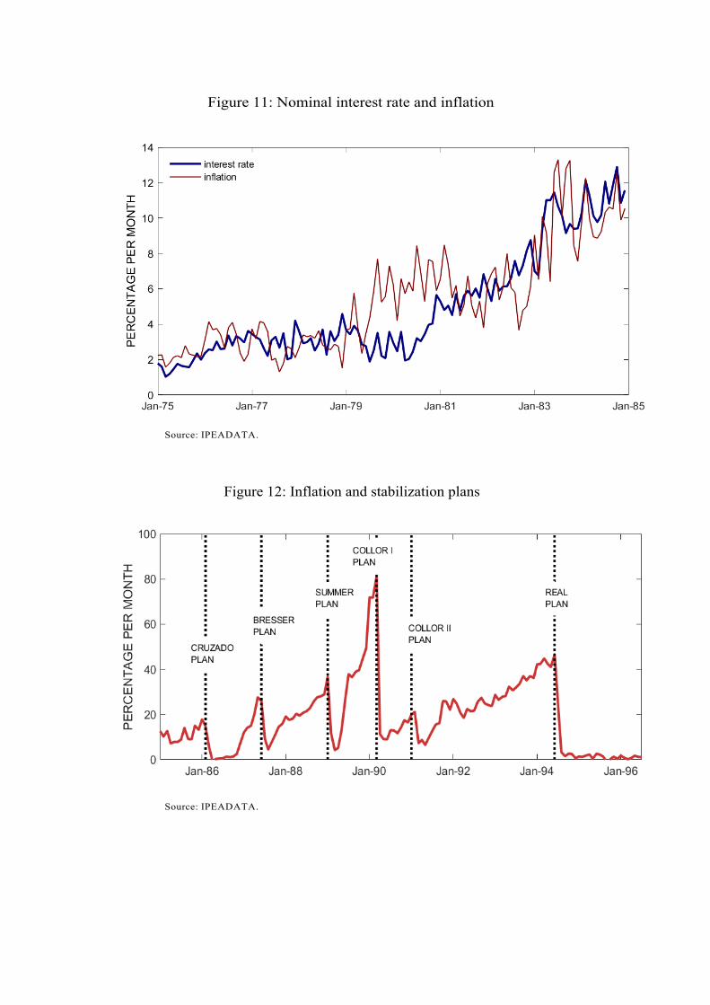
Figure 11: Nominal interest rate and inflation

Source: IPEADATA.

Figure 12: Inflation and stabilization plans

Source: IPEADATA.

Figure 13: International accounts

Source: Central Bank of Brazil and IPEADATA.

Figure 14: Real exchange rate

Source: Central Bank of Brazil, IPEADATA, and Bureau of Labor Statistics.

Figure 15: Interest payments on external debt

Source: Central Bank of Brazil and IPEADATA.

Figure 16: Net external debt of the Central Bank of Brazil

Source: Central Bank of Brazil and IPEADATA.

Figure 17: Real wages

Source: IPEADATA.

Figure 18: Exports and Imports

Source: Central Bank of Brazil and IPEADATA.

Figure 19: Monetary aggregates

Source: IPEADATA.

Figure 20: National Monetary Council (CMN)

Source: Franco (2017) and IPEADATA.

Figure 21: Balance sheet of the Central Bank of Brazil

(a)   Assets

(b)   Liabilities

Source: Central Bank of Brazil.

Figure 22: Transfers from CBB to the government

Source: Central Bank of Brazil, IPEADATA, and authors’ calculations.

Figure 23: Revenues and expenditures after the Real Plan

Source: Central Bank of Brazil, IPEADATA, and authors’ calculations.

C   Data Appendix

This appendix provides the sources of the data used in the paper, compares them to other available data series, and describes the methodology used to compute the government budget constraint as presented in Table 1 of the main text.

C.1   Primary deficit series in Brazil

In Brazil, there are two different sources of data on the public sector primary deficit: the Brazilian Institute of Geography and Statistics (IBGE), and the Central Bank of Brazil (CBB). The data from IBGE are annual and cover the period from 1947 to the present.39 They include the federal government, states, and municipalities, and are published in the national accounts – public sector.40 The IBGE data are based on the executed budget of the government. The data on primary deficit from CBB, on the other hand, are available on an annual frequency since 1985, and on a monthly frequency since January 1991. They include the federal government, states, and municipalities, as well as the central bank and state-owned enterprises (SOEs). We illustrate both (original) series in Figure 24.

There are important differences in the methodology used to compute each of these series. The data from IBGE use the actual data reported in the books of government authorities and can be considered the traditional measure of primary deficit.41 CBB, on the other hand, estimates the primary deficit based on the public sector borrowing requirement. That is, CBB computes the variation of the stock of net debt and money supply from the federal government, central bank, states and municipalities, and SOEs. That variation gives a proxy for the fiscal deficit of the government that includes both interest payments and the primary deficit. CBB then estimates the interest payments based on the characteristics of assets and liabilities and computes the primary deficit as a residual. In Brazil, there is a preference among economists to use the deficit series from CBB after 1985.42 A few factors explain that. First, at the onset of the external debt crisis in the early 1980s, authorities needed to work with recent data, and the statistics on the primary deficit took a long time to be released. CBB, on the other hand, had the ability to compile the debt information for both domestic and external debt in a timely fashion, so it decided to compute its own fiscal statistics based on the public sector borrowing requirements. The second factor is the inclusion of SOEs. The debt series used by CBB covered SOEs, while other deficit series did not. Since SOEs were constantly used by

39From 1947 to 2000, the series can be downloaded from the Estatısticas do Seculo XX from IBGE. We extrapolate it using the annual publications of the public-sector accounts. 40Data on the federal government deficit are also readily available at the website of the Department of the Treasury for the most recent period.

41For example, it uses data from the Balanco Geral da Uniao (Union General Budget) for the federal government.

42See Giambiagi and Alem (2011).

Figure 24: Primary deficit: CBB versus IBGE

Source: Brazilian Institute of Geography and Statistics and Central Bank of Brazil.

the government to implement its economic policies (see main text), that was considered to be a significant advantage. Third, there was a lack of confidence in the capability of the government to report its finances accurately. The National Treasury Secretariat, for example, was only created in 1986.

Even though the paper uses the primary deficit series from CBB after 1985 as many Brazilian economists recommend, we use this appendix to discuss a few points. First, the inclusion or not of SOEs in the primary deficit series does not make a big difference after 1985, especially after the 1990s when most privatizations took place (Figure 24). Second, CBB did not take into account privatizations when estimating primary deficits. In other words, if the government sold some of its assets to finance current expenditures, that would not be captured in the deficit series from CBB. Figure 25a compares both series, with privatization and not, for the period after 1996, which is the year when the data on privatizations used by CBB became available.

Third, CBB does not account for defaults. It estimates interest payments on an accrual basis. So if the government defaulted on its interest payments, CBB would underestimate the primary deficit. The reason is that CBB assumes that the government paid all the interest that was due. Therefore, it would conclude that the government had the resources to pay for them, which must have come from lower primary deficits (or higher surpluses) according to CBB’s methodology. Remember that primary deficit is computed as a residual. But if the government defaulted on the interest payments, then it must be the case that deficits were actually higher than the ones reported by CBB. As the main text mentions, the country accumulated arrears on interest payments on the external debt for many years, especially in the 1990–1994 period. We use the information

Figure 25: Adjustments to primary deficit series from CBB

(a)  Privatization adjustment

(b)  Default adjustment

(c)  Debt recognition adjustment

Source: Brazilian Institute of Geography and Statistics and Central Bank of Brazil.

on the fraction of interest on external debt that were actually paid to correct for both the interest payments and primary deficit series reported by CBB. The difference in the primary deficit series is illustrated in Figure 25b. Unfortunately, we do not have

information regarding defaults on domestic debt. Fourth, CBB does not distinguish “bad assets” from the rest of the government’s

assets. In these cases, CBB might conclude that the government is saving, since it is accumulating more assets, when in reality those assets are worthless (extreme case). One example is the accounts from Bank of Brazil (BB) in CBB’s balance sheet (see main text), that were used to transfer funds from CBB to BB. In Figure 26a we show the magnitude of those transfers given by the variation in their balances. By looking at its own assets, CBB would conclude that it is saving, but those funds were never repaid and represented deficits. We did correct the primary deficit series for the transfers between CBB and BB through those accounts. However, there might be other cases. Imagine, for example, the (hypothetical) case in which the government bails out a public bank by exchanging its “bad assets” that they were holding in their balance sheets. CBB would conclude that there were no surpluses or deficits, since the government is exchanging assets by liabilities in “equal” amount, when in reality there were transfers to finance expenditures.43

Fifth, there are also cases in which there are debt recognitions (skeletons) that enter the debt series. CBB does not include those variations when estimating the primary deficit, but it shows that there were previous deficits that were not taken into account. They are shown in Figure 25c.

Finally, note that the IBGE series also misses the transactions between CBB and BB, so we also need to make that adjustment on the IBGE series for the period in which we use it (before 1985). See Figure 26b.

C.1.1   Implications

As we could see in Figure 24, the difference between both series is significant,

especially around the Real Plan. However, the main conclusion from our analysis does not change, even when we include the adjustments mentioned above. The low-inflation period (after 1994) is characterized by improvements in fiscal balances. Note that both series show primary surpluses after 1998. The main controversy arises in the period surrounding the implementation of the Real Plan. It is usually emphasized that the government switched from large surpluses to large deficits when it was implemented, but given the pitfalls in CBB’s series, one cannot be 100% sure of it. If we look at IBGE’s series instead, we observe the opposite: large deficits before the Real Plan and an improvement right after. But again, this series also has its own pitfalls, so one must be careful when making conclusions based on those observations.

43In other words, the value of those assets in the balance sheet do not represent their true value.

Figure 26: Adjustment regarding Bank of Brazil (BB)

(a)  CBB + BB

(b)  IBGE + BB

Source: Brazilian Institute of Geography and Statistics and Central Bank of Brazil.

C.2   Data sources

Real GDP

Data is from the Brazilian Institute of Geography and Statistics (IBGE). It is annual, from 1947 to 2014, and can be downloaded at http://seriesestatisticas.ibge.gov.br (series SCN53). The series show the percentage variation in volume. We normalize real GDP in 1995 to 100 and use the variation to construct the series of real GDP. We use another data series to extend it until 2016. We use the annual variation in real GDP (reference year 2010) between 2015 and 2016 available at http://ipeadata.gov.br to update the real

GDP series until 2016. We also work with monthly data, so it is useful to construct a monthly series of real

GDP. We assume that the annual values correspond to July values, and use linear interpolation to compute real GDP for the other months.

Price index

We use the General Price Index (IGP) from the Getulio Vargas Foundation. It is com-

posed by: 60% Producer Price Index (IPA), 30% Consumer Price Index (IPC), and 10% Construction Price Index (INCC). Prices are collected from day one to day thirty of the reference month. Series begin in January 1944. The series can be downloaded at http://www.ipeadata.gov.br (IGP-DI - geral - ındice (ago. 1994 = 100)). End-of-period values are computed as the geometric average of IGP-DI in t  and t  + 1. In order to make the IGP-DI consistent with the GDP deflator, we normalize the IGP-DI such that its average in 1995 is equal to the GDP deflator in that year. The GDP deflator in 1995 is equal to the nominal GDP (IPEADATA: Produto interno bruto (PIB) a precos de mercado - referencia 2000) in 1995 divided by 100 (since we normalized real GDP to 100 in 1995).

The IGP-DI is very sensitive to variations in the exchange rate, so Table 4 reports the results using the consumer price index from FIPE, instead.

Table 4: Government budget accounting with IPC-Fipe (% of GDP)

subperiod

Uses

60–64 65–72 73–80 81–94 95-16

(1) interest on domestic debt 0.1 0.0 -0.3 -0.2 3.8 (2) interest on external debt 0.0 0.0 0.4 1.0 0.4 (3) primary deficit 1.1 0.4 0.1 0.3 -2.5 (4) transfers = (5)+(6)+(7)+(8)-(1)-(2)-(3) 0.3 0.5 2.0 0.2 0.0

Sources

(5) domestic debt 0.0 0.3 0.0 0.6 2.4 (6) external debt 0.0 0.0 1.4 -1.7 -1.3 (7) real monetary base -0.2 -0.1 0.0 0.1 0.2 (8) seigniorage 1.6 0.7 0.8 2.2 0.4

Source: Brazilian Institute of Geography and Statistics (IBGE) and Central Bank of Brazil (CBB).

Nominal GDP

Computed by the multiplication of the real GDP series and price index series described

above.

Population

Data is from the Brazilian Institute of Geography and Statistics (IBGE), available at

http://ipeadata.gov.br, for the period 1872 until 2015 at annual frequency. The name of the series is populacao residente. We update the series until 2016 using another series from IBGE available at http://ipeadata.gov.br, “populacao residente - 1◦  de julho - estimativas”. We assume the same growth rate between 2015 and 2016.

Exchange rate

For the exchange rate, we have both average price and end-of-period prices available. We focus on buy price. The series is available at http://ipeadata.gov.br, with the annual series available from 1942 to 2017, and the monthly series from January 1953 to May 2018.

Monetary base

Monthly series from January 1946 to April 2018 from Central Bank (series 1788), and

it can be decomposed between currency issued (series 1786) and banking reserves (series 1787) starting in January 1980. They reflect end-of-period balances and the annual series is constructed based on December values. The monthly series for average monthly balance is also available for the period January 1980 to April 2018 (series 1785), and it can be decomposed between banking reserves (series 1784) and currency issued (1783).

Reserves

Annual series (reservas internacionais) from 1945 to 2017 is available at http://ipeadata.gov.br. The monthly series from December 1970 to May 2018 is available at the Central Bank (series 3546). Domestic Debt

Before 1981, we use the sum of three series: D ıvida Fundada do Governo Federal, debt

securities from federal government, and debt securities from states, available at IPEADATA. After 1981, we use the Dıvida Lıquida do Setor Publico (DLSP) from the Central Bank of Brazil and which is available at IPEADATA.

External Debt

Before 1971, we assume external net debt of the public sector is zero. Between 1971 and 1981, we use data on the public sector external debt related to balance of payments data. After 1981, we use the Dıvida Lıquida do Setor Publico (DLSP) from the Central Bank of Brazil and which is available at IPEADATA.

References Abreu, Marcelo, and R. L. F. Werneck. 2014. “Estabilização, abertura e privatização, 1990-1994.” In A Ordem do Progreso: Dois Séculos de Política Econômica no Brasil, 2nd ed. Edited by Marcelo P. Abreu. Elsevier. Bacha, E. 2003. “Development Economics and Structuralist Macroeconomics: Essays in Honor of Lance Taylor.” Chapt. Brazil's Plano Real: a view from the inside. Cheltenham, UK: Edward Elgar. Bevilaqua, A. S., D. D. Carneiro, M. G. P. Garcia, and R. L. F. Werneck. 2001. “The Structure of Public Sector Debt in Brazil.” RES Working Papers 3121, Inter-American Development Bank, Research Department. Carneiro, Dionísio D. 2014. “Crise e esperança: 1974-1980.” In A Ordem do Progreso: Dois Séculos de Política Econômica no Brasil, 2nd ed. Edited by Marcelo P. Abreu. Elsevier. Carneiro, D. D., and M. G. P. Garcia. 1993. “Capital Flows and monetary control under a domestic currency substitution regime: The recent Brazilian experience.”. Textos para discussão 304, Department of Economics PUC-Rio (Brazil). Carneiro, Dionisio D., and E. Modiano. 2014. “Ajuste externo e desequilíbrio interno: 1980-1984.” In A Ordem do Progreso: Dois Séculos de Política Econômica no Brasil, 2nd ed. Edited by Marcelo P. Abreu. Elsevier. Carvalho, B. S. M., and M. G. P. Garcia. 2008. “Ineffective Controls on Capital Inows under Sophisticated Financial Markets: Brazil in the Ninities.” In Financial Markets Volatility and Performance in Emerging Markets, NBER Chapters. National Bureau of Economic Research, Inc., pp. 29-96. Cati, R. C., M. G. P. Garcia, and P. Perron. 1999. “Unit Roots in the Presence of Abrupt Governmental Interventions with an Application to Brazilian Data.” Journal of Applied Econometrics 14 (1): 27-56. Cerqueira, Ceres A. 2003. Dívida externa brasileira, 2nd ed. Banco Central do Brasil. Costa Neto, Yttrio C. 2004. Bancos oficiais no Brasil: origem e aspectos de seu desenvolvimento. Banco Central do Brasil. Franco, G. 2015. “O Plano Real e a reconstrução da moeda.” Unpublished manuscript. Franco, Gustavo H. B. 2017. “O Conselho Monetário Nacional como Autoridade Monetária: das origens aos dias atuais.” In A Crise Fiscal e Monetária Brasileira. Civilização Brasileira, 2nd ed. Edited by Edmar Bacha. Garcia, M. G. P. 1993. “The Fisher effect in a signal extraction framework: The recent Brazilian experience.”

Journal of Development Economics 41 (1): 71-94. ________. 1996. “Avoiding some costs of inflation and crawling toward hyperinflation: The case of Brazilian domestic currency substitute.” Journal of Development Economics 51 (1): 139-159. Giambiagi, F., and A. Além. 2011. Finanças Públicas. Elsevier. Guardia, E. R. (1992). “Orçamento Público e política fiscal: aspectos institucionais e a experiência recente, 1985-1991.” Universidade de Campinas. Master’s thesis. Gurkayanak, R. S., B. Sack, and J. H. Wright. 2010. “The TIPS Yield Curve and Ination Compensation.” American Economic Journal: Macroeconomics 2 (1): 70-92. International Monetary Fund. 1995. “Guidelines for Fiscal Adjustment.” No 49 in Pamphlet Series. Jaloretto, C. 2005. “Senhoriagem e Financiamento do Setor Público," Universidade de Brasília. Master’s thesis. Lago, Luiz A. C. 2014. “A retomada do crescimento e as distorções do “milagre”: 1967-1974.” In A Ordem do Progreso: Dois Séculos de Política Econômica no Brasil, 2nd ed. Edited by Marcelo P. Abreu. Elsevier. Mesquita, Mário M.C. 2014. “Inflação, Estagnação e ruptura, 1961-1964.” In A Ordem do Progreso: Dois Séculos de Política Econômica no Brasil, 2nd ed. Edited by Marcelo P. Abreu. Elsevier. Modiano, Eduardo M. 2014). “A ópera dos três cruzados, 1985-1990.” In A Ordem do Progreso: Dois Séculos de Política Econômica no Brasil, 2nd ed. Edited by Marcelo P. Abreu. Elsevier. Orenstein, Luiz, and A. C. Sochaczewski. 2014. “Democracia com desenvolvimento: 1956-1961.” In A Ordem do Progreso: Dois Séculos de Política Econômica no Brasil, 2nd ed. Edited by Marcelo P. Abreu. Elsevier. Pastore, A. C. 1995. “Déficit Público, a Sustentabilidade do Crescimento das Dívidas Interna e Externa, Senhoriagem e Inflação: Uma Análise do Regime Monetário Brasileiro.” Revista de Econometria 14 (2): 177-234. ________. 1996. “Por que a Política Monetária perde a eficácia?” Revista de Econometria 50 (3): 281-311. Pedras, Guilherme B. V. 2009. “História da dívida pública no Brasil: de 1964 até os dias atuais.” In Dívida Pública: a experiência brasileira. Edited by Silva, Anderson C., L. O. de Carvalho, and O. L. de Medeiros. Tesouro Nacional. Resende, André L. 2014. “Estabilização e reforma, 1964-1967.” In A Ordem do Progreso: Dois Séculos de Política Econômica no Brasil, 2nd ed. Edited by Marcelo P. Abreu. Elsevier. Rezende, M. 2000. “O Crescimento da Dívida Pública no Período 1970 a 1999.” PUC-Rio, Departamento de Economia. Master’s thesis. Rocha, R. R., and F. Saldanha. 1995. “Fiscal and quasi-fiscal deficit, nominal and real: measurement and policy issues.” Revista Brasileira de Economia 49 (3): 431-466. Silva, Anderson C. 2009. “Origem e história da dívida pública no Brasil até 1963.” In Dívida Pública: a experiência brasileira. Edited by Silva, Anderson C., L. O. de Carvalho, and O. L. de Medeiros. Tesouro

Nacional. Simonsen, M. 1983. “Indexation: Current Theory and the Brazilian Experience.” In Inflation, Debt and Indexation. Edited by Rudiger Dornbusch and Mario H. Simonsen. The MIT Press. Werneck, Rogério L. F. 2014a. “Consolidação da estabilização e reconstrução institucional, 1995-2002.” In A Ordem do Progreso: Dois Séculos de Política Econômica no Brasil, 2nd ed. Edited by Marcelo P. Abreu. Elsevier. _________. 2014b. “Alternância política, redistribuição e crescimento, 2003-2010.” In A Ordem do Progreso: Dois Séculos de Política Econômica no Brasil, 2nd ed. Edited by Marcelo P. Abreu. Elsevier.