Embed Size (px)
Citation preview

WORKING PAPER SERIES
No 4 / 2009
THE EFFECTS OF FISCAL INSTRUMENTS ON THE ECONOMY OF LITHUANIA
By Sigitas Karpavicius
THE EFFECTS OF FISCAL INSTRUMENTS
ON THE ECONOMY OF LITHUANIA
WORKING PAPER SERIESNo 4 / 2009
by Sigitas Karpavicius1
1 University of New South Wales.
E-mail: [email protected] would like to thank two anonymous referees and Igor Vetlov for their very usefulcomments and suggestions. I am solely responsible for any remaining errors.
^

© Lietuvos bankas, 2009Reproduction for educational and non-commercial purposes ispermitted provided that the source is acknowledged.
AddressTotoriu g. 4LT-01121 VilniusLithuaniaTelephone +370 5 268 0132Fax +370 5 212 4423
Internethttp://www.lb.lt
Statement of purposeWorking Papers describe research in progress by the author(s) andare published to stimulate discussion and critical comments.
The Series is managed by Economic Research Division of EconomicsDepartment
The views expressed are those of the author(s) and do notnecessarily represent those of the Bank of Lithuania.
ISSN 2029-0446 (ONLINE)
,
The
Effectsof
FiscalInstruments
onthe
Economy
ofLithuania
/S.K
arpavičius
Contents
Abstract/Santrauka 4
1. Introduction 5
2. Literature Review 6
3. Description of Model 7
4. Results 94.1. Degree of Self-Financing of Tax Cuts . . . . . . . . . . . . . . . . . . 94.2. Impact of Decrease in Statutory Tax Rate . . . . . . . . . . . . . . . 11
4.2.1. Impact of Decrease in Statutory Consumption Tax Rate . . . 114.2.2. Impact of Decrease in Statutory Labor Tax Rate . . . . . . . 124.2.3. Impact of Decrease in Statutory Capital Tax Rate . . . . . . 13
4.3. Impact of Decrease in Government Expenditure . . . . . . . . . . . . 144.4. Impact of Increase in Transfers . . . . . . . . . . . . . . . . . . . . . 154.5. Government Expenditure Multiplier . . . . . . . . . . . . . . . . . . 17
5. Summary and Concluding Remarks 18
A. Derivation of Welfare Measure 20
B. Effective vs. Statutory Tax Rates 22B.1. Value Added Tax . . . . . . . . . . . . . . . . . . . . . . . . . . . . . 22B.2. Labor Tax . . . . . . . . . . . . . . . . . . . . . . . . . . . . . . . . . 23B.3. Capital Tax . . . . . . . . . . . . . . . . . . . . . . . . . . . . . . . . 23
C. Figures and Tables 24
Bibliography 32
List of Bank of Lithuania Working Papers 34
3
Ban
kof
Lith
uani
aW
orki
ngPap
erSe
ries
No
4/
2009 Abstract
The goal of this paper is to examine the dynamic effects of fiscal in-struments in Lithuania on the economy and welfare. In the analysis, acalibrated dynamic stochastic general equilibrium model for Lithuaniais employed. The calculation implies that 9-16 percent of tax cuts areself-financing in the long run. It suggests that the slope of Laffer curvein Lithuanian economy is rather flat. The analysis of effects of differenttax cuts shows that the impact of 1 percentage point permanent decreasein statutory tax rate on gross domestic product is very small (within therange of –0.15 through 0.15 percent in all cases). The estimated gov-ernment expenditure multiplier has a different sign in the long run whenvarious financing sources are used to balance the government budget.
Keywords: fiscal policy, degree of self-financing of tax cuts, impact oftax cuts, government expenditure multiplier.JEL classifications: E62, H24, H25.
SantraukaTaikant kalibruotą Lietuvos ekonomikos dinamini stochastini bendro-
sios pusiausvyros modeli, darbe nagrinejamas fiskaliniu priemoniu poveikisšalies ekonomikai. Gaunama, kad mokesčiu sumažinimas “save kompen-suoja” 9-16 procentu ilgu laikotarpiu. Taip pat nustatoma, kad mokesčiustatutiniu tarifu sumažinimas 1 procentiniu punktu turi nedaug itakosšalies bendrajam vidaus produktui (nuo –0.15 iki 0.15 procento, priklau-somai nuo mokesčio). Apskaičiuotas vyriausybes išlaidu multiplikatoriusturi skirtingus ženklus ilgu laikotarpiu. Multiplikatoriaus reikšme prik-lauso nuo vyriausybes biudžeto papildomo finansavimo šaltinio.
Pagrindiniai žodžiai : fiskaline politika, mokesčiu tarifo sumažinimas, vyriau-sybes išlaidu multiplikatorius.
4

The
Effectsof
FiscalInstruments
onthe
Economy
ofLithuania
/S.K
arpavičius
1. Introduction
The economic policy is implemented using instruments of monetary and fiscal policy.The combination of instruments helps the authority achieve certain objectives, in-crease welfare of citizens as well as ensure the sustainable economic growth. Seekinga relative price stability over a longer period, in 1994 Lithuanian currency litas waspegged to the US dollar. Because of the expanding economical relationship withthe members of the European Union and prospective membership in the EuropeanUnion, in 2002 the litas was pegged to the euro. The analysis shows that the cur-rency board arrangement in Lithuania was beneficial (see Kuodis, 2003). However,the peg implies that economic policy in Lithuania is mainly determined by the fiscalmeans. Thus, to know the impact of individual fiscal instrument on the economyand welfare in both short run and long run is a must.
This paper examines the effects of the fiscal instruments, namely labor tax, cap-ital tax, consumption tax, transfers to households, and government spending, onLithuanian economy and welfare assuming balanced government budget. The out-come should help identify the best compensating mechanisms of tax cuts, choosethe appropriate fiscal instruments to achieve desired objectives, and so determinethe best policy. Furthermore, government expenditure multiplier and the degree ofself-financing of tax cuts, i.e. to what extent a tax cut pays for itself, are calculatedin this paper.
In the analysis, a calibrated dynamic stochastic general equilibrium (DSGE) modelfor Lithuanian economy is used. The model is based on microeconomic foundations.Woodford (2003, 1 ch.) documents that micro-founded models are superior to themacroeconometric models for two reasons. First, in the macroeconometric models theexpectations of future variables are determined by the current and lagged observablestate variables. However, the relationship is expected to alter in case of the changein the policy of government. This problem can be tackled by using the first orderconditions to determine the optimal behavior of private sector. These conditionsimply the expected evolution of endogenous variables, and their structure remainsconstant when the government’s policy changes. Second advantage of micro-foundedmodel is their ability to calculate the impact on welfare that is indicated by theutility function of the private agent in case of changes in the government’s policyor any other shock. Due to these reasons, the effects of fiscal policy as well asoptimal taxation on labor market, economy, and welfare are mostly analyzed usingdynamic general equilibrium models (for example, Chamley, 1985, Prescott, 2004).Recently DSGE models have become very popular among macroeconomists. Smets& Wouters (2003) conclude that “the current generation of New-Keynesian DSGE
5

Ban
kof
Lith
uani
aW
orki
ngPap
erSe
ries
No
4/
2009 models with sticky prices and wages and endogenous persistence in consumption
and investment are able to capture the main features of the euro area data quitewell, as long as one is willing to entertain enough structural shocks to capture thestochastics.” Therefore, using DSGE model documented in Karpavičius (2008) thatis based on microeconomic foundations and is properly calibrated for Lithuanianeconomy in this exercise is advantageous.
Our model-based simulation results imply that 9-16 percent of tax cuts are self-financing in the long run. It means that the slope of Laffer curve in Lithuanianeconomy is rather flat. The analysis of effects of different tax cuts shows that theimpact of 1 p.p. permanent decrease in statutory tax rate on GDP is very small(within the range of –0.15 through 0.15 percent in all cases). The results indicatethat there is no unique recipe how to decrease the rate of a tax since the effectson welfare, price level, and GDP are different when different financing means areused to balance the government budget. The adequate financing sources need to bechosen to achieve desired objectives, for example, to increase GDP or welfare. Theestimated government expenditure multiplier has different values in the long runwhen various financing sources are used to balance the government budget. On thecontrary to Baxter & King (1993), government expenditure multiplier is lower than1 when additional government purchases are financed by lump-sum taxes. All in all,the impact of tax cuts and government expenditure multiplier are relatively small.Consequently, it is likely that fiscal instruments, analyzed in this paper, alone arenot able substantially to affect Lithuanian economy.
The paper is organized as follows. Section 2 summarizes the existing literature.The model used is outlined in Section 3. Section 4 provides the results and theirexplanation. Finally, Section 5 concludes.
2. Literature Review
There is a relatively large empirical literature on the effects of fiscal policy andoptimal taxation. It is impossible to acknowledge the vast literature on the subjectbut several studies relevant to the topic of this paper should be reviewed.
Two recent studies, Cardia et al. (2003) and Prescott (2004), analyze the impactof labor tax. Prescott (2004) finds that marginal labor tax rate plays a key rolein the differences in labor supply for the major advanced industrial countries. Theauthor states that the welfare gains from reducing the effective labor tax rate inthe higher tax rate countries are larger. Since in Lithuania effective labor incometax is relatively low (see Karpavičius, 2008), it is likely that there is no significant
6
The
Effectsof
FiscalInstruments
onthe
Economy
ofLithuania
/S.K
arpavičius
improvement on welfare when labor tax rate is reduced. Cardia et al. (2003) findthat a reduction of 10 p.p. in the labor tax rate would increase weekly hours workedby 4.5% in Germany, 9.9% in Canada, 12.8-18.0% in the USA and 14.5% in Japan.
Employing DSGE models, Mankiw & Weinzierl (2005) and Trabandt & Uhlig(2006) find that in the US economy approximately one fifth of the capital tax cutand one half of the labor tax cut are self-financing. The results of Trabandt &Uhlig (2006) indicate that in the EU-15 economy one half of labor tax cut and 85percent of capital tax cut are self-financing. The findings indicate that tax cut isable to generate economic growth that can offset a portion of loss of governmentincome. Authors explain that the degree of self-financing depends on the positionof a country on its Laffer curve. The tax-cuts in EU-15 pay more for themselvesbecause the distortions in EU-15 are higher.
Christ (1968) analyzes the impact of financing source on government expendituremultiplier. He argues that the government expenditure multiplier cannot be esti-mated “until it is decided how to finance the purchases”. The author finds that themultiplier is greater than 1 in case the expenditure is not financed by the increase intaxes, else it is below 1 but still positive. Baxter & King (1993), utilizing the neo-classical dynamic general equilibrium model, analyze the effects of changes in fiscalpolicy on macroeconomic activity. The authors find that government expendituremultiplier is likely to exceed 1 in the short run and in the long run (when addi-tional government purchases are financed by lump-sum taxation). However, theyemphasize the importance of financing source of the increase in government spend-ing: tax-financed government spending leads to the decrease in output. Devereux& Love (1995) obtain similar results. In addition, the authors document that thepermanent increase in government spending that is financed with lump-sum taxesreduces social welfare.
3. Description of Model
To examine the impact of the proposed fiscal reform on Lithuanian economy andwelfare, the quarterly model of Karpavičius (2008) is employed. The model is prop-erly calibrated for recent Lithuanian data.1 The model is an extended version of the
1Lithuanian version of the paper that includes the derivation of the model, the steady state for-mulas and log-linearized equations is available upon request. Model description in English isavailable in Karpavičius & Vetlov (2008). The only difference of models in Karpavičius & Vet-lov (2008) and this paper is capital accumulation process. In this paper, capital accumulationprocess incorporates certain capital adjustment costs, whereas in Karpavičius & Vetlov (2008)the process includes investment adjustment costs. In this paper, capital accumulation process is
described as Kt = (1−δ) exp(−ω)Kt−1 +It− Φ exp(ω)2
(Kt−Kt−1)2
Kt−1, where Kt is capital stock, δ is
7
Ban
kof
Lith
uani
aW
orki
ngPap
erSe
ries
No
4/
2009 New-Keynesian DSGE open economy model with sticky prices and nominal wages
and is developed following Dam & Linaa (2005), Kollmann (2002), Smets & Wouters(2003).
A small open economy model features five sectors: households, intermediate goodsproducers, final goods producers, fiscal and monetary authorities. The economy pro-duces a homogeneous non-tradable final good and a continuum of tradable interme-diate goods. Therefore, the international trade takes place in intermediate goods.Households maximize the intertemporal utility as a function of consumption and la-bor, subject to an intertemporal budget constraint and taking as given the externalconsumption habit. Each household is a monopolistic supplier of a differentiatedlabor service. This leads to an explicit wage equation with Calvo (1983) stickiness.Households own all domestic producers and capital stock. Households rent capitalto the domestic firms and decide how much to invest in capital stock given cer-tain capital adjustment costs. Households temporally can increase their expenditurebeyond current income due to the foreign borrowing. Labor and capital used inthe production of intermediate goods are perfectly immobile internationally. Thereis a monopolistic competition in intermediate goods markets. Intermediate goodsproducers produce differentiated intermediate goods which are aggregated and soldunder imperfect competition to final goods producers at home and abroad. Interme-diate goods producers reoptimise prices infrequently á la Calvo (1983), but can setdifferent prices in the domestic and foreign market. Domestic final goods producertransforms the intermediate product into a homogeneous final good and sells in aperfectly competitive market. Fiscal authority collects three types of distortionarytaxes (labor, capital and consumption taxes) and has two kinds of expenditures,government consumption and transfers to households.2 In the benchmark model,government expenditure on final consumption goods is endogenous and all taxes andtransfers are exogenous.3 However, when it is needed, government expenditure isexogenous and any tax rate (or transfers) is endogenous. The government budgetis balanced each period. The interest rate at which households can borrow fundsabroad depends on foreign interest rate and net foreign asset position. Foreign ex-change rate is constant, however, the central bank is able to revaluate or devaluatethe domestic currency. The appropriate welfare measures are derived in AppendixA.
capital depreciation rate, ω denotes the labor-augmenting technological (deterministic) change,It is investment, and Φ denotes the coefficient of capital adjustment costs that is calibratedto the value of 7.2. In addition, model in this paper assumes that government does not useborrowing to balance its budget.
2If transfers are negative, they are equivalent to lump-sum taxes paid to the government.3This assumption is feasible as the authority changes tax laws rather frequently and in the 3rd
quarter of each year the additional incomes are redistributed to achieve fiscal deficit targets (in1999, the expenditure of government was reduced).
8

The
Effectsof
FiscalInstruments
onthe
Economy
ofLithuania
/S.K
arpavičius
4. Results
In the analysis, the impulse responses of variables to unexpected cuts in differenttaxes and changes in government expenditure using the procedure described in Uhlig(1999) are computed.
The following section discusses the results. First of all, the degree of self-financingof capital, labor, and consumption tax cuts is obtained. Thereafter, the impact of 1p.p. permanent decrease in each tax statutory rate is calculated. Further, the impactof 1 p.p. of GDP permanent decrease in government expenditure and effect of 0.1p.p. of GDP permanent reduction in transfers to households are analyzed. Finally,government expenditure multiplier is computed (in case of permanent increase ingovernment expenditure).
4.1. Degree of Self-Financing of Tax Cuts
The degree of self-financing of tax cuts is calculated following the procedure presentedin Mankiw & Weinzierl (2005) and Trabandt & Uhlig (2006). The dynamic andstatic effects are considered. In the model, Gt denotes government expenditureon final consumption goods. The static scoring, Gstatic, is obtained from cuttingsteady state tax level in log-linearized government budget constraint, while keepingother variables constant. Whereas the dynamic scoring, Gdynamic
t , is the impulseresponse of government expenditure to the unexpected permanent decrease in taxrate. Therefore, the degree of self-financing at time t can be written as:
Gstatic −Gdynamict
Gstatic.
In addition, government pays transfers to households. Transfers amount to a fixedpercentage of GDP. For analysis purposes, transfers to households can be consideredas lump-sum taxes. Thus, total tax revenue of government is equal to governmentexpenditure on final consumption goods, Gt.
The analysis shows that 14% of a consumption tax cut is self-financing (see Figure1). The main “source” of self-financing is the positive impact on consumption whereasthe effects on employment and economic growth are minor (see Table 1 in AppendixC).
Approximately 16% of labor tax cut is self-financing. According to the findings,labor tax cut has the highest degree of self-financing in Lithuanian economy in bothlong run and short run. Additional revenue from consumption tax is the main factor
9

Ban
kof
Lith
uani
aW
orki
ngPap
erSe
ries
No
4/
2009
0%
2%
4%
6%
8%
10%
12%
14%
16%
18%
-1 3 7 11 15 19 23 27 31 35 39 43 47 51 55 59 63 67 71 75 79 83 87 91 95 99
Quarters
Consumption tax Capital tax
Labor tax Lump-sum tax (-transfers)
Figure 1: The degree of self-financing of tax cuts
of self-financing.
The degree of self-financing of capital tax cut is approximately 12% in the longrun but it is twice smaller in the short run. Slow convergence of the degree of self-financing to its terminal value is observed as it takes time to adjust capital stockto its new optimal level. The degree of self-financing of lump-sum tax cut is higherin the short run (up to 13%) and lower in the long run (9%). The degree of self-financing of lump-sum tax cut is lower than degree of self-financing of other tax cutsin the long run because lump-sum tax is not distortionary; therefore, its cut causeslower incentives for households to work more or to invest more in capital.
The results imply that the degree of self-financing of tax cuts in Lithuanian econ-omy is smaller than one in EU-15 and US economies (Mankiw & Weinzierl, 2005,Trabandt & Uhlig, 2006). There are at least two possible reasons for this issue.Firstly, it is likely that the distortions of taxation in Lithuania are lower than in EU-15 and US economies. Secondly, DSGE models used in this paper and in Trabandt &Uhlig (2006) are quite different. Trabandt & Uhlig (2006) employ relatively simplemodel; however, the model used in this paper is open economy model and featuresseveral nominal and real frictions. The findings suggest that the slope of Laffer curvein Lithuanian economy is rather flat. If the tax rates were higher in Lithuania, theanalysis would lead to the higher degree of self-financing of tax cuts (see Figure 8 inAppendix C).
10

The
Effectsof
FiscalInstruments
onthe
Economy
ofLithuania
/S.K
arpavičius
The main factor of self-financing for all cases is the additional government incomefrom consumption tax (due to increased consumption of households). Moreover, thesmall impact on the economic activity leads to the modest increase in governmentincome from other taxes. Therefore, during the 1st year the proportions of labor taxcut, consumption tax cut, and lump-sum tax cut coincide.
The results, presented in this Section, might be useful to policymakers since thefindings indicate that Laffer curve in Lithuanian economy is relatively flat thus theadditional taxation would not create a lot of distortions. Similarly, tax cuts do notlead to significantly smaller distortions. Therefore, the opportunity of “free lunch”almost does not exist. The results presented in this Section are obtained assumingthat the decrease in tax rate would not affect the level of shadow economy. Sincethe tax cuts are likely to alleviate tax evasion, the effective degree of self-financingcan be slightly higher (see Karpavičius & Vetlov, 2008).
4.2. Impact of Decrease in Statutory Tax Rate
Further in this Section, the effects of 1 p.p. decrease in statutory consumption tax(value added tax), labor tax (personal income tax) and capital tax (capital incometax) rates are presented in case of different scenarios. The interrelation between thestatutory and effective tax rates is computed in Appendix B. The outcome shouldhelp identify the best compensating means in case of tax cuts. Beside the effects onGDP and welfare measures, the impact on price level (before consumption tax) isanalyzed. The latter is important due to the recently rising inflation in Lithuania.The findings suggest that the variations in financing source of a particular tax cutcould lead to different effects on variables of interest.
4.2.1. Impact of Decrease in Statutory Consumption Tax Rate
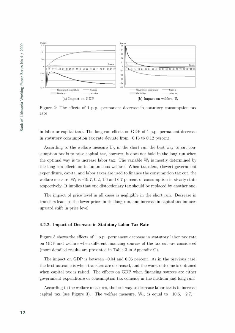
Figure 2 depicts the effects of 1 p.p. permanent decrease in statutory consumptiontax rate on GDP and welfare when different financing sources of the tax cut are con-sidered (more detailed results are presented in Table 2 in Appendix C). All dynamicresponses are shown as percent deviations from a balanced growth path.
The positive impact on GDP is observed when the permanent decrease in statutoryconsumption tax rate is compensated by the decrease in transfers to households (orthe increase in lump-sum taxes). GDP is slightly positively affected in the mediumrun, but is unaffected in the long run when financing source of tax cut is the decreasedgovernment consumption. GDP is negatively affected when the financing sources arecapital and labor taxes (i.e. the consumption tax cut is financed by either increase
11
Ban
kof
Lith
uani
aW
orki
ngPap
erSe
ries
No
4/
2009
tauk 3.9 0.57 0.45 0.36 0.31 0.27 0.23 0.217.4 0.00 0.00 0.01 0.01 0.02
-0.15
-0.1
-0.05
0
0.05
0.1
0.15
-1 4 9 14 19 24 29 34 39 44 49 54 59 64 69 74 79 84 89 94 99
Quarter
Percent
Government expenditure Trasfers
Capital tax Labor tax
(a) Impact on GDP
-0.5
-0.4
-0.3
-0.2
-0.1
0
0.1
0.2
0.3
0.4
0.5
-1 4 9 14 19 24 29 34 39 44 49 54 59 64 69 74 79 84 89 94 99
Quarter
Percent
Government expenditure Trasfers
Capital tax Labor tax
(b) Impact on welfare, Ut
Figure 2: The effects of 1 p.p. permanent decrease in statutory consumption taxrate
in labor or capital tax). The long-run effects on GDP of 1 p.p. permanent decreasein statutory consumption tax rate deviate from –0.13 to 0.12 percent.
According to the welfare measure Ut, in the short run the best way to cut con-sumption tax is to raise capital tax, however, it does not hold in the long run whenthe optimal way is to increase labor tax. The variable Wt is mostly determined bythe long-run effects on instantaneous welfare. When transfers, (lower) governmentexpenditure, capital and labor taxes are used to finance the consumption tax cut, thewelfare measure Wt is –19.7, 0.2, 1.6 and 6.7 percent of consumption in steady staterespectively. It implies that one distortionary tax should be replaced by another one.
The impact of price level in all cases is negligible in the short run. Decrease intransfers leads to the lower prices in the long run, and increase in capital tax inducesupward shift in price level.
4.2.2. Impact of Decrease in Statutory Labor Tax Rate
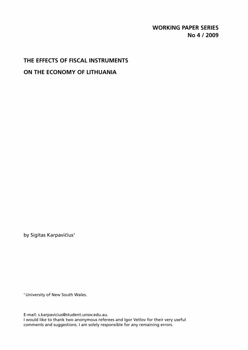
Figure 3 shows the effects of 1 p.p. permanent decrease in statutory labor tax rateon GDP and welfare when different financing sources of the tax cut are considered(more detailed results are presented in Table 3 in Appendix C).
The impact on GDP is between –0.04 and 0.06 percent. As in the previous case,the best outcome is when transfers are decreased, and the worst outcome is obtainedwhen capital tax is raised. The effects on GDP when financing sources are eithergovernment expenditure or consumption tax coincide in the medium and long run.
According to the welfare measures, the best way to decrease labor tax is to increasecapital tax (see Figure 3). The welfare measure, Wt, is equal to –10.6, –2.7, –
12

The
Effectsof
FiscalInstruments
onthe
Economy
ofLithuania
/S.K
arpavičius
-0.06
-0.04
-0.02
0
0.02
0.04
0.06
0.08
-1 4 9 14 19 24 29 34 39 44 49 54 59 64 69 74 79 84 89 94 99
Quarter
Percent
Government expenditure Trasfers
Capital tax Consumption tax
(a) Impact on GDP
-0.2
-0.15
-0.1
-0.05
0
0.05
0.1
0.15
0.2
-1 4 9 14 19 24 29 34 39 44 49 54 59 64 69 74 79 84 89 94 99
Quarter
Percent
Government expenditure Trasfers
Capital tax Consumption tax
(b) Impact on welfare, Ut
Figure 3: The effects of 1 p.p. permanent decrease in statutory labor tax rate
2.6, and –2.0 percent of consumption in steady state when the change in transfers,consumption tax, government expenditure, and capital tax are used to balance thegovernment budget respectively.
The effects on price level are also diverse. The decrease in transfers leads to themost negative impact on prices (–0.06 percent in the long run), and the increase incapital tax determines 0.04 percent increase in price level. When consumption tax isused to balance government budget, the impact on price level is negligible, but oneneeds to consider that unlike the calculation of consumer price index, in the modelthe change in price level does not include directly the change in consumption taxrate.
4.2.3. Impact of Decrease in Statutory Capital Tax Rate
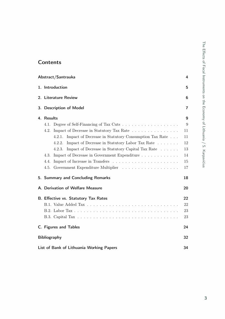
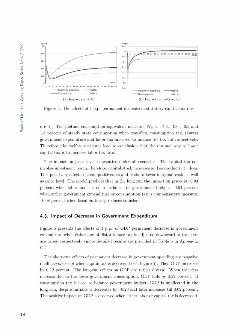
Figure 4 shows the effects of 1 p.p. permanent decrease in statutory capital tax rateon GDP and welfare when different financing sources of the tax cut are considered(more detailed results are given in Table 4 in Appendix C).
When capital tax rate is reduced, GDP is positively affected under all scenarios.The capital tax cut implies the permanent positive change in the optimal capital-output ratio, ultimately this leads to the higher GDP. The impact varies from 0.03to 0.08 percent in the long run. When labor tax is used to balance the governmentbudget, the impact is 0.03 percent. The effects on GDP coincide (are equal to 0.04percent) when the tax cut is finance either by the decrease in government expenditureor by higher consumption tax. GDP is upward shifted by 0.08 percent when transfersare compensatory measure.
The effects on welfare are negative in the short run under all scenarios (see Fig-
13
Ban
kof
Lith
uani
aW
orki
ngPap
erSe
ries
No
4/
2009
0
0.02
0.04
0.06
0.08
0.1
-1 4 9 14 19 24 29 34 39 44 49 54 59 64 69 74 79 84 89 94 99
Quarter
Percent
Government expenditure Trasfers
Consumption tax Labor tax
(a) Impact on GDP
-0.35
-0.3
-0.25
-0.2
-0.15
-0.1
-0.05
0
0.05
-1 4 9 14 19 24 29 34 39 44 49 54 59 64 69 74 79 84 89 94 99Quarter
Percent
Government expenditure Trasfers
Consumption tax Labor tax
(b) Impact on welfare, Ut
Figure 4: The effects of 1 p.p. permanent decrease in statutory capital tax rate
ure 4). The lifetime consumption equivalent measure, Wt, is –7.5, –0.6, –0.5 and1.8 percent of steady state consumption when transfers, consumption tax, (lower)government expenditure and labor tax are used to finance the tax cut respectively.Therefore, the welfare measures lead to conclusion that the optimal way to lowercapital tax is to increase labor tax rate.
The impact on price level is negative under all scenarios. The capital tax cutinvokes investment boom; therefore, capital stock increases and so productivity does.This positively affects the competitiveness and leads to lower marginal costs as wellas price level. The model predicts that in the long run the impact on prices is –0.03percent when labor tax is used to balance the government budget; –0.04 percentwhen either government expenditure or consumption tax is compensatory measure;–0.08 percent when fiscal authority reduces transfers.
4.3. Impact of Decrease in Government Expenditure
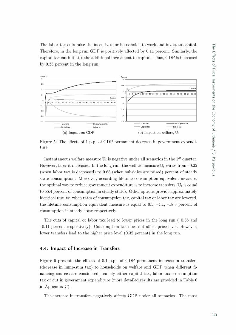
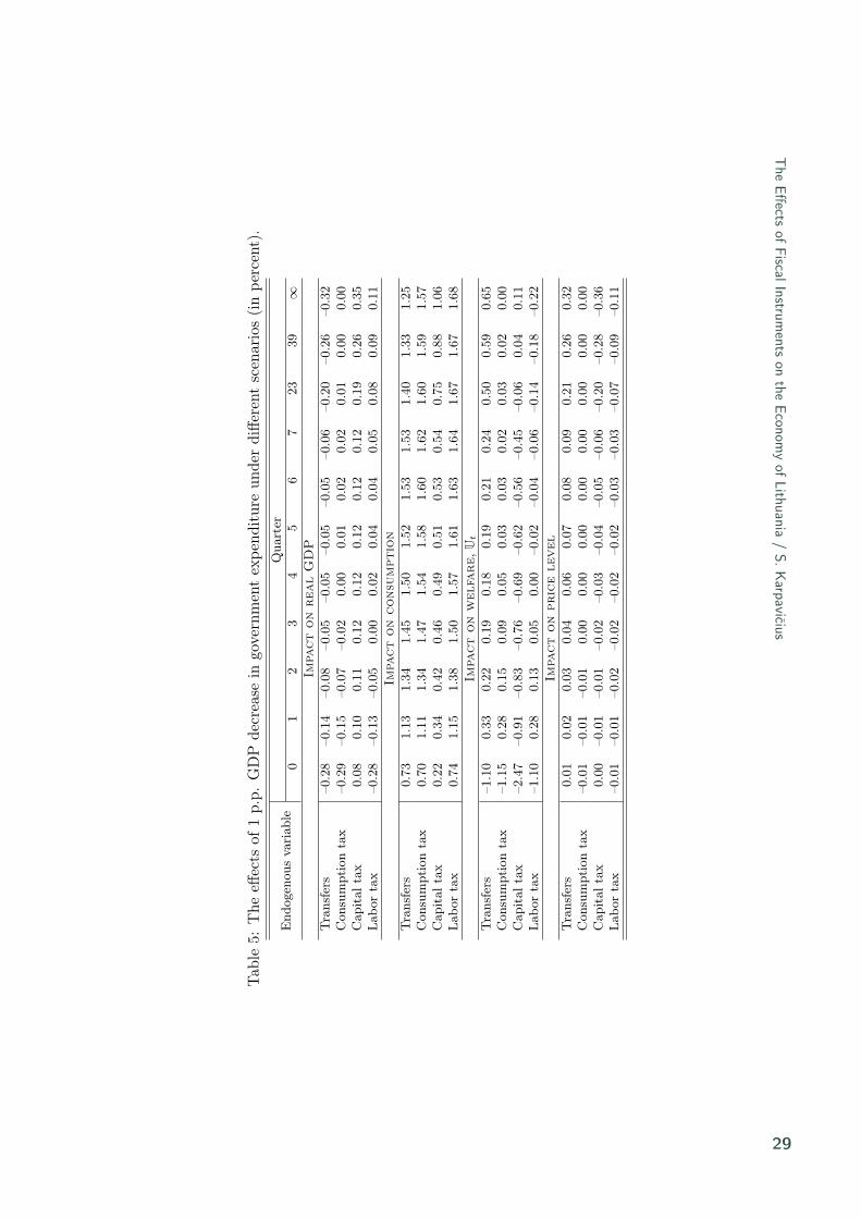
Figure 5 presents the effects of 1 p.p. of GDP permanent decrease in governmentexpenditure when either any of distortionary tax is adjusted downward or transfersare raised respectively (more detailed results are provided in Table 5 in AppendixC).
The short-run effects of permanent decrease in government spending are negativein all cases, except when capital tax is decreased (see Figure 5). Then GDP increasesby 0.12 percent. The long-run effects on GDP are rather diverse. When transfersincrease due to the lower government consumption, GDP falls by 0.32 percent. Ifconsumption tax is used to balance government budget, GDP is unaffected in thelong run, despite initially it decreases by –0.29 and later increases till 0.02 percent.The positive impact on GDP is observed when either labor or capital tax is decreased.
14
The
Effectsof
FiscalInstruments
onthe
Economy
ofLithuania
/S.K
arpavičius
The labor tax cuts raise the incentives for households to work and invest to capital.Therefore, in the long run GDP is positively affected by 0.11 percent. Similarly, thecapital tax cut initiates the additional investment to capital. Thus, GDP is increasedby 0.35 percent in the long run.
-0.4
-0.3
-0.2
-0.1
0
0.1
0.2
0.3
0.4
-1 4 9 14 19 24 29 34 39 44 49 54 59 64 69 74 79 84 89 94 99
Quarter
Percent
Transfers Consumption tax
Capital tax Labor tax
(a) Impact on GDP
-2.5
-2
-1.5
-1
-0.5
0
0.5
1
-1 4 9 14 19 24 29 34 39 44 49 54 59 64 69 74 79 84 89 94 99
Quarter
Percent
Transfers Consumption tax
Capital tax Labor tax
(b) Impact on welfare, Ut
Figure 5: The effects of 1 p.p. of GDP permanent decrease in government expendi-ture
Instantaneous welfare measure Ut is negative under all scenarios in the 1st quarter.However, later it increases. In the long run, the welfare measure Ut varies from –0.22(when labor tax is decreased) to 0.65 (when subsidies are raised) percent of steadystate consumption. Moreover, according lifetime consumption equivalent measure,the optimal way to reduce government expenditure is to increase transfers (Ut is equalto 55.4 percent of consumption in steady state). Other options provide approximatelyidentical results: when rates of consumption tax, capital tax or labor tax are lowered,the lifetime consumption equivalent measure is equal to 0.5, –4.1, –18.3 percent ofconsumption in steady state respectively.
The cuts of capital or labor tax lead to lower prices in the long run (–0.36 and–0.11 percent respectively). Consumption tax does not affect price level. However,lower transfers lead to the higher price level (0.32 percent) in the long run.
4.4. Impact of Increase in Transfers
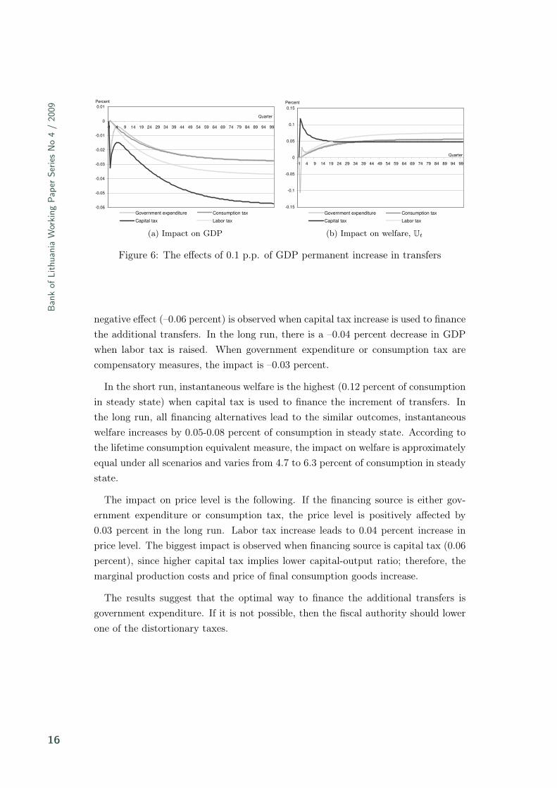
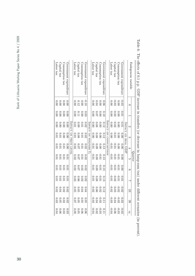
Figure 6 presents the effects of 0.1 p.p. of GDP permanent increase in transfers(decrease in lump-sum tax) to households on welfare and GDP when different fi-nancing sources are considered, namely either capital tax, labor tax, consumptiontax or cut in government expenditure (more detailed results are provided in Table 6in Appendix C).
The increase in transfers negatively affects GDP under all scenarios. The most
15
Ban
kof
Lith
uani
aW
orki
ngPap
erSe
ries
No
4/
2009
-0.06
-0.05
-0.04
-0.03
-0.02
-0.01
0
0.01
-1 4 9 14 19 24 29 34 39 44 49 54 59 64 69 74 79 84 89 94 99
Quarter
Percent
Government expenditure Consumption tax
Capital tax Labor tax
(a) Impact on GDP
-0.15
-0.1
-0.05
0
0.05
0.1
0.15
-1 4 9 14 19 24 29 34 39 44 49 54 59 64 69 74 79 84 89 94 99
Quarter
Percent
Government expenditure Consumption tax
Capital tax Labor tax
(b) Impact on welfare, Ut
Figure 6: The effects of 0.1 p.p. of GDP permanent increase in transfers
negative effect (–0.06 percent) is observed when capital tax increase is used to financethe additional transfers. In the long run, there is a –0.04 percent decrease in GDPwhen labor tax is raised. When government expenditure or consumption tax arecompensatory measures, the impact is –0.03 percent.
In the short run, instantaneous welfare is the highest (0.12 percent of consumptionin steady state) when capital tax is used to finance the increment of transfers. Inthe long run, all financing alternatives lead to the similar outcomes, instantaneouswelfare increases by 0.05-0.08 percent of consumption in steady state. According tothe lifetime consumption equivalent measure, the impact on welfare is approximatelyequal under all scenarios and varies from 4.7 to 6.3 percent of consumption in steadystate.
The impact on price level is the following. If the financing source is either gov-ernment expenditure or consumption tax, the price level is positively affected by0.03 percent in the long run. Labor tax increase leads to 0.04 percent increase inprice level. The biggest impact is observed when financing source is capital tax (0.06percent), since higher capital tax implies lower capital-output ratio; therefore, themarginal production costs and price of final consumption goods increase.
The results suggest that the optimal way to finance the additional transfers isgovernment expenditure. If it is not possible, then the fiscal authority should lowerone of the distortionary taxes.
16
The
Effectsof
FiscalInstruments
onthe
Economy
ofLithuania
/S.K
arpavičius
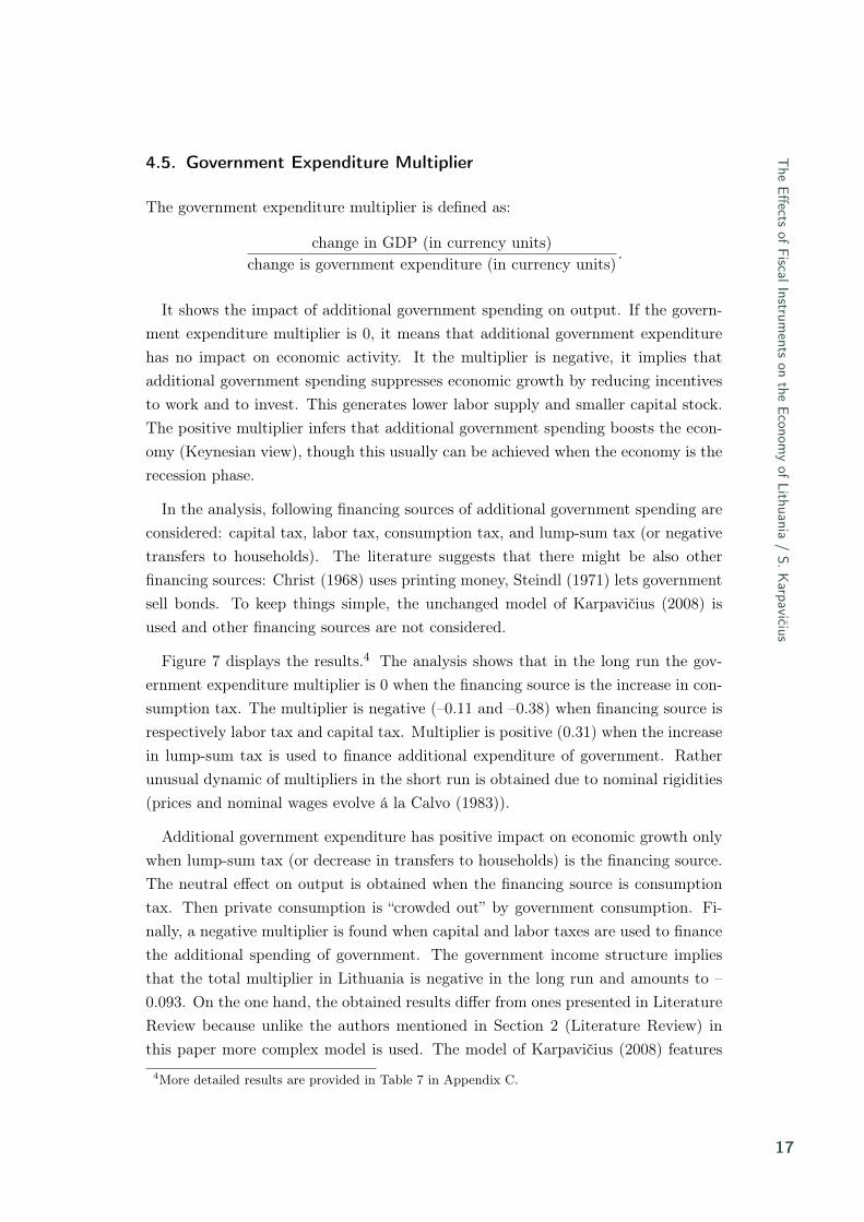
4.5. Government Expenditure Multiplier
The government expenditure multiplier is defined as:
change in GDP (in currency units)change is government expenditure (in currency units)
.
It shows the impact of additional government spending on output. If the govern-ment expenditure multiplier is 0, it means that additional government expenditurehas no impact on economic activity. It the multiplier is negative, it implies thatadditional government spending suppresses economic growth by reducing incentivesto work and to invest. This generates lower labor supply and smaller capital stock.The positive multiplier infers that additional government spending boosts the econ-omy (Keynesian view), though this usually can be achieved when the economy is therecession phase.
In the analysis, following financing sources of additional government spending areconsidered: capital tax, labor tax, consumption tax, and lump-sum tax (or negativetransfers to households). The literature suggests that there might be also otherfinancing sources: Christ (1968) uses printing money, Steindl (1971) lets governmentsell bonds. To keep things simple, the unchanged model of Karpavičius (2008) isused and other financing sources are not considered.
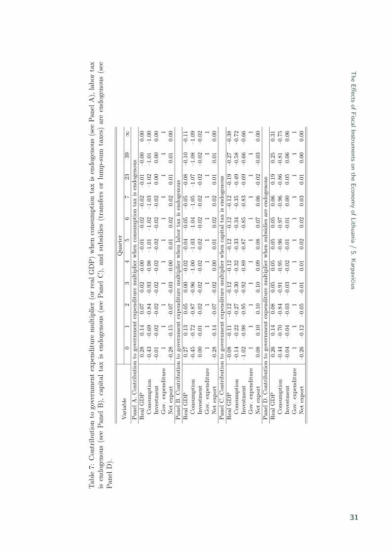
Figure 7 displays the results.4 The analysis shows that in the long run the gov-ernment expenditure multiplier is 0 when the financing source is the increase in con-sumption tax. The multiplier is negative (–0.11 and –0.38) when financing source isrespectively labor tax and capital tax. Multiplier is positive (0.31) when the increasein lump-sum tax is used to finance additional expenditure of government. Ratherunusual dynamic of multipliers in the short run is obtained due to nominal rigidities(prices and nominal wages evolve á la Calvo (1983)).
Additional government expenditure has positive impact on economic growth onlywhen lump-sum tax (or decrease in transfers to households) is the financing source.The neutral effect on output is obtained when the financing source is consumptiontax. Then private consumption is “crowded out” by government consumption. Fi-nally, a negative multiplier is found when capital and labor taxes are used to financethe additional spending of government. The government income structure impliesthat the total multiplier in Lithuania is negative in the long run and amounts to –0.093. On the one hand, the obtained results differ from ones presented in LiteratureReview because unlike the authors mentioned in Section 2 (Literature Review) inthis paper more complex model is used. The model of Karpavičius (2008) features
4More detailed results are provided in Table 7 in Appendix C.
17

Ban
kof
Lith
uani
aW
orki
ngPap
erSe
ries
No
4/
2009
-0.4
-0.3
-0.2
-0.1
0
0.1
0.2
0.3
0.4
-1 5 11 17 23 29 35 41 47 53 59 65 71 77 83 89 95
Quarters
Lump-sum tax (-subsidy) Consumption tax Labor tax Capital tax
Figure 7: The government expenditure multiplier in case of different financing sources
nominal and real rigidities, in addition, households can use external financing sources(foreign debt) to maximize their utility. On the other hand, this paper emphasizesthe importance of choice of financing source as it is documented in the existingliterature.
5. Summary and Concluding Remarks
This paper assesses the effectiveness of the fiscal instruments in Lithuania. Theresults imply that the degree of self-financing of tax cuts in Lithuanian economy issmaller than the ones in EU-15 and US economies. There are at least two possiblereasons for this. Firstly, it is likely that the distortions of taxation in Lithuania arelower than in EU-15 and US economies. Secondly, DSGE models used in this paperand in Trabandt & Uhlig (2006) are quite different. Trabandt & Uhlig (2006) employrelatively simple model; however, the model used in this paper is open economy modeland features several nominal and real frictions.
The calculation implies that 9-16 percent of tax cuts are self-financing in the longrun. This means that the slope of Laffer curve in Lithuanian economy is ratherflat. The analysis of effects of different tax cuts shows that the impact of 1 p.p.permanent decrease in statutory tax rate on GDP is very small (within the range of–0.15 through 0.15 percent in all cases). The results indicate that there is no unique
18

The
Effectsof
FiscalInstruments
onthe
Economy
ofLithuania
/S.K
arpavičius
recipe how to decrease the rate of a tax since the effects on welfare, price level, andGDP are different when different financing means are used to balance the governmentbudget. As a conclusion, the adequate financing sources need to be chosen to achievedesirable objectives, for example, to increase GDP or welfare.
The estimated government expenditure multiplier has different values in the longrun when different financing sources are used to balance the government budget. Onthe contrary to Baxter & King (1993), government expenditure multiplier is lowerthan 1 when additional government purchases are financed by lump-sum taxes. Allin all, the impact of tax cuts and government expenditure multiplier are relativelysmall. Consequently, one can state that fiscal instruments, analyzed in this paper,alone are not able substantially to affect Lithuanian economy.
The main disadvantage of the method used in this paper is considered to be thetype of the model.5 DSGE models are generally devised for mature economies thatare in the vicinity of the steady state of their economic development. In this case,the analysis of impulse responses and simulations is reasonable and policy-relevant.In contrast, Lithuanian economy might be decades away from its steady state whichcould create some doubts regarding the reliability of results. At least one model-ing issue help mitigate this problem. The model used in this paper incorporateslabor-augmenting technological (deterministic) growth. Thus, the numeric values ofimpulse responses to shocks show percent deviations not from steady state but froma balanced growth path (certain upward sloping trend). Notwithstanding with theproblems discussed above, the use of DSGE model let us obtain dynamic impact ofshocks on economic variables and utilize other advantages of micro-founded models.
Several important extensions to this analysis readily suggest themselves. Poten-tial extensions of the paper involve the analysis of effects of fiscal policy assumingthe presence of rule-of-thumb (non-Ricardian) consumers, and the impact of pre-announced tax reform. Another possible extension is to introduce tax evasion in theanalysis. Furthermore, the employed model could be extended to allow householdswith finite planning horizons. All these issues would improve the understanding ofeffectiveness of fiscal policy in Lithuania and are left for future research.
5I thank the referee for pointing this out to me.
19
Ban
kof
Lith
uani
aW
orki
ngPap
erSe
ries
No
4/
2009 A. Derivation of Welfare Measure
Welfare analysis is based upon the computation of non-stochastic instantaneous util-ity function of a household. In the model, households also derive utility from apublic good which is provided by government, i.e. government expenditure is notjust a waste of resources for households. Therefore, the utility function, Ut, is ex-tended by adding government consumption that is adjusted to its steady state value:
Ut =(Ct − hCt−1)
1−σC
1− σC− L1+σL
t
1 + σL+
G
C
(Gt − hGt−1)1−σC
1− σC,
where Ct denotes private final consumption goods, Gt denotes public final con-sumption goods, Lt is labor supply, σC is the inverse of intertemporal elasticity ofsubstitution of consumption, σL is the inverse of elasticity of labor supply, h denotesthe habit formation parameter, C and G are respectively private and public finalconsumption goods in steady state. Note that the changes (in real terms) in privateconsumption and changes in government consumption affect the household’s utilityequally. However, household takes public goods as given and is not able to optimizetheir quantity.
The utility function is log-linearized around consumption in steady state:
Ut ≈ U + CUt.
Therefore, the measure of welfare, Ut, shows the changes of utility of household interms of consumption in steady state:
Ut =[(1− h)C
]−σC Ct − h[(1− h)C
]−σC Ct−1 −(L)1+σL
CLt +
+(
G
C
)2 [(1− h)G
]−σC Gt −(
G
C
)2
h[(1− h)G
]−σC Gt−1.
Ut can be considered as the measurement of instantaneous welfare gains in termsof consumption in steady state. In addition, the respective literature (for example,Prescott, 2004) suggests to use the lifetime consumption equivalent measure. It showsthe percentage of consumption today and in all future periods must be increased inorder households would be indifferent to proposed policy change.
20

The
Effectsof
FiscalInstruments
onthe
Economy
ofLithuania
/S.K
arpavičius
In this paper, the lifetime consumption equivalent measure, Wt, is given by:
Wt =∞∑
t=0
βtUt,
where β denotes the subjective discount factor.
21
Ban
kof
Lith
uani
aW
orki
ngPap
erSe
ries
No
4/
2009 B. Effective vs. Statutory Tax Rates
In this Section, the relationships between the effective tax rates (the rates in themodel) and the statutory tax rates that are determined in the law are computed.
B.1. Value Added Tax
Households’ real consumption expenditure in the model is given by:
(1 + τ ct )Ct,
where τ ct is the effective consumption tax.
However, in the real economy it can be expressed by the following equation:
(1 + V AT )at + (1 + V AT )(ED + bt) + ct, where
V AT is value added tax, ED is excise duty, at are goods subject to V AT , bt aregoods subject to V AT and ED, ct are goods free from tax, and at + bt + ct = Ct.
Thus:(1 + V AT )at + (1 + V AT )(ED + bt) + ct = (1 + τ c
t )Ct. (1)
From Equation 1, one can get the following equations:
at + bt
Ct=
τ ct − (1 + V AT )
(EDCt
)V AT
,
τ ct = V AT
(at + bt
Ct
)+ (1 + V AT )
(ED
Ct
). (2)
The main statutory VAT rate in Lithuania is 0.18. In the model, τ ct = 0.162 (see
Karpavičius, 2008). The value of EDCt
can be obtained from the national accountsand the statistics of government budget. In 2006, it was approximately equal to 0.44.Plugging the values for V AT , τ c
t , and EDCt
into Equation 2, one can get that:
at + bt
Ct≈ 0.611.
Plugging this value into Equation 2, one can get that 1 percentage point changein VAT is equivalent to:
• 0.44 p.p. change in τ ct , if V AT = 0, else
22

The
Effectsof
FiscalInstruments
onthe
Economy
ofLithuania
/S.K
arpavičius
• 0.655 p.p. change in τ ct .
B.2. Labor Tax
In the model government income from labor tax is τ ltWtLt where Wt denotes real
(gross) wage, τ lt is the effective tax rates on labor income. The effective labor tax
rate can be written as:τ lt =
x · PIT ·WtLt
WtLt + at, where (3)
at is the non-taxable income, PIT is the statutory personal income tax rate, andx · PIT stands for adjusted statutory PIT rate (the adjustment is needed due taxconcessions and the fact that 30% of revenues from personal income tax are transferedto the Compulsory Health Insurance Fund).
According to Karpavičius (2008), labor income in the model is equivalent to thesum of the following national accounts: D.1 Compensation of employees, D.2 Taxesproduction and imports, and B.3n Mixed income, net. It is assumed that only com-pensation of employees is subject to PIT. Using the statistical data for 2003-2006,one can get that: WtLt
WtLt+at≈ 0.66.
Since τ lt = 0.091 in Karpavičius (2008), and the statutory PIT rate till the middle
of 2006 was 0.33, using Equation 3 one can get that x ≈ 0.42. Therefore, 1 p.p. ofPIT is equivalent to 0.276 p.p. of τ l
t .
B.3. Capital Tax
The effective capital tax, τkt , rate can be written as:
τkt =
CIT · at
at + bt, where
CIT is the statutory rate of corporate income tax,at is the tax base, bt is the non-taxable corporate income. According to Karpavičius (2008), τk
t = 0.051, and thestatutory CIT rate is 0.15, thus 1 p.p. of CIT is equivalent to 0.34 p.p. of τk
t .
23

Ban
kof
Lith
uani
aW
orki
ngPap
erSe
ries
No
4/
2009 C. Figures and Tables
0
0.05
0.1
0.15
0.2
0.25
0.3
0.35
0.4
0 3 6 9 12 15 18 21 24 27 30 33 36 39 42 45 48 51 54 57 60
Quarter
tau^c=0.162 tau^c=0.3 tau^c=0.5
(a) Consumption tax
-0.1
-0.05
0
0.05
0.1
0.15
0.2
0.25
0 3 6 9 12 15 18 21 24 27 30 33 36 39 42 45 48 51 54 57 60
Quarter
tau^l=0.091 tau^l=0.3 tau^l=0.5
(b) Labor tax
0
0.05
0.1
0.15
0.2
0.25
0.3
0 3 6 9 12 15 18 21 24 27 30 33 36 39 42 45 48 51 54 57 60
Quarter
tau^k=0.051 tau^k=0.3 tau^k=0.5
(c) Capital tax
Figure 8: The degree of self-financing of tax cuts for different steady-state tax rates
24

The
Effectsof
FiscalInstruments
onthe
Economy
ofLithuania
/S.K
arpavičius
Tab
le1:
Con
trib
utio
nto
the
degr
eeof
self-
finan
cing
ofco
nsum
ptio
nta
xcu
t(s
eePan
elA
),la
bor
tax
cut
(see
Pan
elB
),ca
pita
lta
xcu
t(s
eePan
elC
),an
dlu
mp-
sum
tax
cut
(see
Pan
elD
).Q
uart
erV
aria
ble
01
23
45
67
2339
∞Pan
elA
.Con
trib
utio
nto
the
degr
eeof
self-
finan
cing
ofco
nsum
ptio
nta
xcu
tSt
atic
–1–1
–1–1
–1–1
–1–1
–1–1
–1D
ynam
ic–0
.95
–0.9
1–0
.88
–0.8
7–0
.86
–0.8
6–0
.86
–0.8
6–0
.86
–0.8
6–0
.86
cons
umpt
ion
tax
–0.9
3–0
.90
–0.8
8–0
.87
–0.8
6–0
.86
–0.8
6–0
.86
–0.8
6–0
.86
–0.8
6la
bor
tax
–0.0
10.
000.
000.
000.
000.
000.
000.
000.
000.
000.
00ca
pita
lta
x–0
.01
–0.0
10.
000.
000.
000.
000.
000.
000.
000.
000.
00lu
mp-
sum
tax
(–tran
sfer
s)0.
000.
000.
000.
000.
000.
000.
000.
000.
000.
000.
00D
egre
eof
self-
finan
cing
0.05
0.09
0.12
0.13
0.14
0.14
0.14
0.14
0.14
0.14
0.14
Pan
elB
.Con
trib
utio
nto
the
degr
eeof
self-
finan
cing
ofla
bor
tax
cut
Stat
ic–1
–1–1
–1–1
–1–1
–1–1
–1–1
Dyn
amic
–0.9
5–0
.91
–0.8
8–0
.87
–0.8
6–0
.85
–0.8
5–0
.85
–0.8
5–0
.85
–0.8
4co
nsum
ptio
n0.
070.
100.
120.
130.
140.
140.
140.
150.
150.
150.
15la
bor
tax
–1.0
0–1
.00
–1.0
0–1
.00
–1.0
0–1
.00
–1.0
0–1
.00
–1.0
0–1
.00
–1.0
0ca
pita
lta
x–0
.01
–0.0
10.
000.
000.
000.
000.
000.
000.
000.
000.
00lu
mp-
sum
tax
(–tran
sfer
s)0.
000.
000.
000.
000.
000.
000.
000.
000.
000.
000.
00D
egre
eof
self-
finan
cing
0.05
0.09
0.12
0.13
0.14
0.15
0.15
0.15
0.15
0.15
0.16
Pan
elC
.Con
trib
utio
nto
the
degr
eeof
self-
finan
cing
ofca
pita
ltax
cut
Stat
ic–1
–1–1
–1–1
–1–1
–1–1
–1–1
Dyn
amic
–0.9
7–0
.96
–0.9
5–0
.95
–0.9
4–0
.94
–0.9
4–0
.94
–0.9
1–0
.90
–0.8
8co
nsum
ptio
nta
x0.
020.
030.
040.
050.
050.
050.
050.
050.
070.
090.
10la
bor
tax
0.00
0.00
0.00
0.00
0.00
0.00
0.00
0.00
0.00
0.01
0.01
capi
talta
x–1
.00
–1.0
0–0
.99
–0.9
9–0
.99
–0.9
9–0
.99
–0.9
9–0
.99
–0.9
9–0
.98
lum
p-su
mta
x(–
tran
sfer
s)0.
000.
000.
000.
000.
000.
000.
000.
000.
000.
000.
00D
egre
eof
self-
finan
cing
0.03
0.04
0.05
0.05
0.06
0.06
0.06
0.06
0.09
0.10
0.12
Pan
elD
.Con
trib
utio
nto
the
degr
eeof
self-
finan
cing
oflu
mp-
sum
tax
cut
Stat
ic–1
–1–1
–1–1
–1–1
–1–1
–1–1
Dyn
amic
–0.9
6–0
.91
–0.8
9–0
.87
–0.8
7–0
.87
–0.8
7–0
.87
–0.8
9–0
.90
–0.9
1co
nsum
ptio
nta
x0.
060.
100.
120.
130.
130.
140.
140.
140.
120.
120.
11la
bor
tax
–0.0
10.
000.
000.
000.
000.
000.
000.
000.
00–0
.01
–0.0
1ca
pita
lta
x–0
.01
–0.0
10.
000.
000.
000.
000.
000.
00–0
.01
–0.0
1–0
.01
lum
p-su
mta
x(–
tran
sfer
s)–1
–1–1
–1–1
–1–1
–1–1
–1–1
Deg
ree
ofse
lf-fin
anci
ng0.
040.
090.
110.
130.
130.
130.
130.
130.
110.
100.
09
25

Ban
kof
Lith
uani
aW
orki
ngPap
erSe
ries
No
4/
2009
Table
2:T
heeffects
of1
p.p.consum
ptiontax
cutsunder
differentscenarios
(inpercent).
Quarter
Endogenous
variable0
12
34
56
723
39∞
Impac
ton
rea
lG
DP
Governm
entexpenditure
–0.11–0.05
–0.02–0.01
0.000.01
0.010.01
0.000.00
0.00Transfers
(lump-sum
tax)0.00
0.000.01
0.010.02
0.020.03
0.030.07
0.090.12
Capitaltax
–0.13–0.09
–0.06–0.05
–0.04–0.04
–0.04–0.04
–0.06–0.09
–0.13Labor
tax0.00
0.000.00
0.00–0.01
–0.01–0.01
–0.01–0.03
–0.03–0.04
Impac
ton
consu
mpt
ion
Governm
entexpenditure
0.270.41
0.490.54
0.560.57
0.580.58
0.570.57
0.56Transfers
(lump-sum
tax)0.00
0.010.01
0.010.02
0.020.03
0.030.07
0.090.12
Capitaltax
0.190.29
0.340.37
0.380.39
0.390.38
0.310.25
0.18Labor
tax0.00
0.000.00
–0.01–0.01
–0.01–0.01
–0.01–0.02
–0.03–0.04
Impac
ton
welfa
re,U
t
Governm
entexpenditure
–0.440.12
0.060.03
0.020.01
0.010.01
0.010.01
0.00Transfers
(lump-sum
tax)0.00
–0.01–0.02
–0.04–0.05
–0.06–0.07
–0.08–0.17
–0.20–0.23
Capitaltax
0.490.43
0.350.30
0.260.23
0.210.19
0.03–0.01
–0.04Labor
tax0.00
0.000.01
0.010.02
0.020.02
0.030.06
0.070.08
Impac
ton
price
level
Governm
entexpenditure
0.000.00
0.000.00
0.000.00
0.000.00
0.000.00
0.00Transfers
(lump-sum
tax)0.00
–0.01–0.01
–0.02–0.02
–0.03–0.03
–0.03–0.07
–0.09–0.12
Capitaltax
0.000.00
0.000.01
0.010.01
0.020.02
0.070.10
0.13Labor
tax0.00
0.000.00
0.010.01
0.010.01
0.010.02
0.030.04
26

The
Effectsof
FiscalInstruments
onthe
Economy
ofLithuania
/S.K
arpavičius
Tab
le3:
The
effec
tsof
1p.
p.la
bor
tax
cuts
unde
rdi
ffere
ntsc
enar
ios
(in
perc
ent)
.Q
uart
erE
ndog
enou
sva
riab
le0
12
34
56
723
39∞
Impa
ct
on
rea
lG
DP
Gov
ernm
ent
expe
ndit
ure
–0.0
4–0
.02
–0.0
10.
000.
000.
010.
010.
010.
010.
010.
02Tra
nsfe
rs(l
ump-
sum
tax)
0.00
0.00
0.00
0.01
0.01
0.01
0.01
0.02
0.04
0.05
0.06
Cap
ital
tax
–0.0
5–0
.03
–0.0
2–0
.02
–0.0
1–0
.01
–0.0
1–0
.01
–0.0
2–0
.02
–0.0
4C
onsu
mpt
ion
tax
0.00
0.00
0.00
0.00
0.00
0.00
0.00
0.00
0.01
0.01
0.02
Impa
ct
on
consu
mpt
ion
Gov
ernm
ent
expe
ndit
ure
0.11
0.17
0.20
0.22
0.23
0.23
0.24
0.24
0.24
0.24
0.24
Tra
nsfe
rs(l
ump-
sum
tax)
0.00
0.00
0.01
0.01
0.01
0.01
0.01
0.02
0.04
0.05
0.06
Cap
ital
tax
0.07
0.12
0.14
0.15
0.16
0.16
0.16
0.16
0.13
0.11
0.09
Con
sum
ptio
nta
x0.
000.
000.
000.
000.
000.
000.
000.
000.
010.
010.
02Im
pact
on
wel
fare,
Ut
Gov
ernm
ent
expe
ndit
ure
–0.1
80.
050.
020.
010.
000.
00–0
.01
–0.0
1–0
.02
–0.0
3–0
.03
Tra
nsfe
rs(l
ump-
sum
tax)
0.00
–0.0
1–0
.01
–0.0
2–0
.03
–0.0
3–0
.04
–0.0
4–0
.09
–0.1
1–0
.13
Cap
ital
tax
0.20
0.17
0.14
0.12
0.10
0.09
0.07
0.06
–0.0
1–0
.03
–0.0
5C
onsu
mpt
ion
tax
0.00
0.00
0.00
–0.0
1–0
.01
–0.0
1–0
.01
–0.0
1–0
.02
–0.0
3–0
.03
Impa
ct
on
pric
ele
vel
Gov
ernm
ent
expe
ndit
ure
0.00
0.00
0.00
0.00
0.00
0.00
0.00
0.00
–0.0
1–0
.01
–0.0
2Tra
nsfe
rs(l
ump-
sum
tax)
0.00
0.00
–0.0
1–0
.01
–0.0
1–0
.01
–0.0
2–0
.02
–0.0
4–0
.05
–0.0
6C
apit
alta
x0.
000.
000.
000.
000.
000.
000.
000.
000.
020.
030.
04C
onsu
mpt
ion
tax
0.00
0.00
0.00
0.00
0.00
0.00
0.00
0.00
–0.0
1–0
.01
–0.0
2
27

Ban
kof
Lith
uani
aW
orki
ngPap
erSe
ries
No
4/
2009
Table
4:T
heeffects
of1
p.p.capitaltax
cutsunder
differentscenarios
(inpercent).
Quarter
Endogenous
variable0
12
34
56
723
39∞
Impac
ton
rea
lG
DP
Governm
entexpenditure
0.010.01
0.010.01
0.010.01
0.010.02
0.020.03
0.04Transfers
(lump-sum
tax)0.05
0.030.03
0.020.02
0.020.02
0.020.05
0.060.08
Consum
ptiontax
0.050.03
0.020.02
0.010.01
0.010.01
0.020.03
0.04Labor
tax0.05
0.030.02
0.020.01
0.010.01
0.010.01
0.020.03
Impac
ton
consu
mpt
ion
Governm
entexpenditure
0.030.04
0.050.06
0.060.06
0.070.07
0.100.11
0.13Transfers
(lump-sum
tax)–0.06
–0.10–0.12
–0.12–0.13
–0.13–0.13
–0.12–0.08
–0.06–0.02
Consum
ptiontax
–0.06–0.10
–0.12–0.13
–0.14–0.14
–0.14–0.14
–0.11–0.09
–0.06Labor
tax–0.07
–0.10–0.12
–0.13–0.14
–0.14–0.14
–0.14–0.12
–0.10–0.08
Impac
ton
welfa
re,U
t
Governm
entexpenditure
–0.32–0.11
–0.11–0.10
–0.09–0.08
–0.07–0.06
–0.010.01
0.01Transfers
(lump-sum
tax)–0.17
–0.16–0.13
–0.12–0.11
–0.10–0.10
–0.09–0.07
–0.07–0.07
Consum
ptiontax
–0.17–0.15
–0.13–0.11
–0.09–0.08
–0.07–0.07
–0.010.00
0.01Labor
tax–0.17
–0.15–0.12
–0.10–0.09
–0.07–0.06
–0.060.01
0.030.04
Impac
ton
price
level
Governm
entexpenditure
0.000.00
0.000.00
0.00–0.01
–0.01–0.01
–0.03–0.04
–0.04Transfers
(lump-sum
tax)0.00
0.00–0.01
–0.01–0.01
–0.01–0.02
–0.02–0.05
–0.07–0.08
Consum
ptiontax
0.000.00
0.000.00
0.00–0.01
–0.01–0.01
–0.03–0.04
–0.04Labor
tax0.00
0.000.00
0.000.00
0.000.00
0.00–0.02
–0.02–0.03
28
The
Effectsof
FiscalInstruments
onthe
Economy
ofLithuania
/S.K
arpavičius
Tab
le5:
The
effec
tsof
1p.
p.G
DP
decr
ease
ingo
vern
men
tex
pend
itur
eun
der
diffe
rent
scen
ario
s(i
npe
rcen
t).
Qua
rter
End
ogen
ous
vari
able
01
23
45
67
2339
∞Im
pact
on
rea
lG
DP
Tra
nsfe
rs–0
.28
–0.1
4–0
.08
–0.0
5–0
.05
–0.0
5–0
.05
–0.0
6–0
.20
–0.2
6–0
.32
Con
sum
ptio
nta
x–0
.29
–0.1
5–0
.07
–0.0
20.
000.
010.
020.
020.
010.
000.
00C
apit
alta
x0.
080.
100.
110.
120.
120.
120.
120.
120.
190.
260.
35Lab
orta
x–0
.28
–0.1
3–0
.05
0.00
0.02
0.04
0.04
0.05
0.08
0.09
0.11
Impa
ct
on
consu
mpt
ion
Tra
nsfe
rs0.
731.
131.
341.
451.
501.
521.
531.
531.
401.
331.
25C
onsu
mpt
ion
tax
0.70
1.11
1.34
1.47
1.54
1.58
1.60
1.62
1.60
1.59
1.57
Cap
ital
tax
0.22
0.34
0.42
0.46
0.49
0.51
0.53
0.54
0.75
0.88
1.06
Lab
orta
x0.
741.
151.
381.
501.
571.
611.
631.
641.
671.
671.
68Im
pact
on
wel
fare,
Ut
Tra
nsfe
rs–1
.10
0.33
0.22
0.19
0.18
0.19
0.21
0.24
0.50
0.59
0.65
Con
sum
ptio
nta
x–1
.15
0.28
0.15
0.09
0.05
0.03
0.03
0.02
0.03
0.02
0.00
Cap
ital
tax
–2.4
7–0
.91
–0.8
3–0
.76
–0.6
9–0
.62
–0.5
6–0
.45
–0.0
60.
040.
11Lab
orta
x–1
.10
0.28
0.13
0.05
0.00
–0.0
2–0
.04
–0.0
6–0
.14
–0.1
8–0
.22
Impa
ct
on
pric
ele
vel
Tra
nsfe
rs0.
010.
020.
030.
040.
060.
070.
080.
090.
210.
260.
32C
onsu
mpt
ion
tax
–0.0
1–0
.01
–0.0
10.
000.
000.
000.
000.
000.
000.
000.
00C
apit
alta
x0.
00–0
.01
–0.0
1–0
.02
–0.0
3–0
.04
–0.0
5–0
.06
–0.2
0–0
.28
–0.3
6Lab
orta
x–0
.01
–0.0
1–0
.02
–0.0
2–0
.02
–0.0
2–0
.03
–0.0
3–0
.07
–0.0
9–0
.11
29
Ban
kof
Lith
uani
aW
orki
ngPap
erSe
ries
No
4/
2009 T
able6:
The
effectsof
0.1p.p.
GD
Pincrease
intransfers
(ordecrease
inlum
p-sumtax)
underdifferent
scenarios(in
percent).Q
uarterE
ndogenousvariable
01
23
45
67
2339
∞Im
pact
on
rea
lG
DP
Governm
entexpenditure
–0.03–0.01
–0.010.00
0.000.00
0.00–0.01
–0.02–0.02
–0.03C
onsumption
tax0.00
0.000.00
0.000.00
–0.01–0.01
–0.01–0.02
–0.02–0.03
Capitaltax
–0.03–0.02
–0.02–0.01
–0.01–0.01
–0.01–0.02
–0.03–0.04
–0.06Labor
tax0.00
0.000.00
0.00–0.01
–0.01–0.01
–0.01–0.02
–0.03–0.04
Impac
ton
consu
mpt
ion
Governm
entexpenditure
0.060.10
0.120.12
0.130.13
0.130.13
0.120.11
0.11C
onsumption
tax0.00
0.000.00
0.000.00
–0.01–0.01
–0.01–0.02
–0.02–0.03
Capitaltax
0.040.07
0.080.08
0.090.09
0.090.08
0.060.04
0.02Labor
tax0.00
0.000.00
0.00–0.01
–0.01–0.01
–0.01–0.02
–0.03–0.04
Impac
ton
welfa
re
Ut
Governm
entexpenditure
–0.100.03
0.020.02
0.020.02
0.020.02
0.040.05
0.06C
onsumption
tax0.00
0.000.01
0.010.01
0.010.02
0.020.04
0.050.06
Capitaltax
0.120.11
0.090.08
0.070.07
0.070.06
0.050.05
0.05Labor
tax0.00
0.000.01
0.010.02
0.020.02
0.030.05
0.070.08
Impac
ton
price
level
Governm
entexpenditure
0.000.00
0.000.00
0.000.01
0.010.01
0.020.02
0.03C
onsumption
tax0.00
0.000.00
0.000.01
0.010.01
0.010.02
0.020.03
Capitaltax
0.000.00
0.000.01
0.010.01
0.010.01
0.040.05
0.06Labor
tax0.00
0.000.00
0.010.01
0.010.01
0.010.02
0.030.04
30
The
Effectsof
FiscalInstruments
onthe
Economy
ofLithuania
/S.K
arpavičius
Tab
le7:
Con
trib
utio
nto
gove
rnm
ent
expe
ndit
ure
mul
tipl
ier
(or
real
GD
P)
whe
nco
nsum
ptio
nta
xis
endo
geno
us(s
eePan
elA
),la
bor
tax
isen
doge
nous
(see
Pan
elB
),ca
pita
lta
xis
endo
geno
us(s
eePan
elC
),an
dsu
bsid
ies
(tra
nsfe
rsor
lum
p-su
mta
xes)
are
endo
geno
us(s
eePan
elD
).Q
uart
erV
aria
ble
01
23
45
67
2339
∞Pan
elA
.Con
trib
utio
nto
gove
rnm
ent
expe
ndit
ure
mul
tipl
ier
whe
nco
nsum
ptio
nta
xis
endo
geno
usR
ealG
DP
0.28
0.14
0.07
0.02
–0.0
0–0
.01
–0.0
2–0
.02
–0.0
1–0
.00
0.00
Con
sum
ptio
n–0
.43
–0.6
9–0
.84
–0.9
3–0
.98
–1.0
1–1
.02
–1.0
3–1
.02
–1.0
1–1
.00
Inve
stm
ent
–0.0
1–0
.02
–0.0
2–0
.02
–0.0
2–0
.02
–0.0
2–0
.02
0.00
0.00
0.00
Gov
.ex
pend
itur
e1
11
11
11
11
11
Net
expo
rt–0
.28
–0.1
5–0
.07
–0.0
3–0
.00
0.01
0.02
0.02
0.01
0.01
0.00
Pan
elB
.Con
trib
utio
nto
gove
rnm
ent
expe
ndit
ure
mul
tipl
ier
whe
nla
bor
tax
isen
doge
nous
Rea
lGD
P0.
270.
130.
050.
00–0
.02
–0.0
4–0
.05
–0.0
5–0
.08
–0.1
0–0
.11
Con
sum
ptio
n–0
.45
–0.7
2–0
.87
–0.9
6–1
.00
–1.0
3–1
.04
–1.0
5–1
.07
–1.0
8–1
.09
Inve
stm
ent
0.00
–0.0
1–0
.02
–0.0
2–0
.02
–0.0
2–0
.02
–0.0
2–0
.02
–0.0
2–0
.02
Gov
.ex
pend
itur
e1
11
11
11
11
11
Net
expo
rt–0
.28
–0.1
4–0
.07
–0.0
20.
000.
010.
020.
020.
010.
010.
00Pan
elC
.Con
trib
utio
nto
gove
rnm
ent
expe
ndit
ure
mul
tipl
ier
whe
nca
pita
ltax
isen
doge
nous
Rea
lGD
P–0
.08
–0.1
1–0
.12
–0.1
2–0
.12
–0.1
2–0
.12
–0.1
2–0
.19
–0.2
7–0
.38
Con
sum
ptio
n–0
.14
–0.2
2–0
.27
–0.3
0–0
.32
–0.3
3–0
.34
–0.3
5–0
.49
–0.5
8–0
.72
Inve
stm
ent
–1.0
2–0
.98
–0.9
5–0
.92
–0.8
9–0
.87
–0.8
5–0
.83
–0.6
9–0
.66
–0.6
6G
ov.
expe
ndit
ure
11
11
11
11
11
1N
etex
port
0.08
0.10
0.10
0.10
0.09
0.08
0.07
0.06
–0.0
2–0
.03
0.00
Pan
elD
.Con
trib
utio
nto
gove
rnm
ent
expe
ndit
ure
mul
tipl
ier
whe
nsu
bsid
ies
are
endo
geno
usR
ealG
DP
0.26
0.14
0.08
0.05
0.05
0.05
0.05
0.06
0.19
0.25
0.31
Con
sum
ptio
n–0
.44
–0.7
0–0
.84
–0.9
1–0
.95
–0.9
6–0
.97
–0.9
6–0
.86
–0.8
1–0
.75
Inve
stm
ent
–0.0
4–0
.04
–0.0
3–0
.03
–0.0
2–0
.01
–0.0
10.
000.
050.
060.
06G
ov.
expe
ndit
ure
11
11
11
11
11
1N
etex
port
–0.2
6–0
.12
–0.0
5–0
.01
0.01
0.02
0.02
0.03
0.01
0.00
0.00
31

Ban
kof
Lith
uani
aW
orki
ngPap
erSe
ries
No
4/
2009 Bibliography
Baxter, Marianne and King, Robert G. (1993). “Fiscal policy in general equilibrium”,American Economic Review 83(3), 315–334.
Calvo, Guillermo A. (1983). “Staggered prices in a utility-maximizing framework”,Journal of Monetary Economics 12(3), 383–398.
Cardia, Emanuela; Kozhaya, Norma and Ruge-Murcia, Francisco J. (2003). “Distor-tionary taxation and labor supply”, Journal of Money, Credit and Banking 35(3),351–373.
Chamley, Christophe (1985). “Efficient tax reform in a dynamic model of generalequilibrium”, The Quarterly Journal of Economics 100(2), 335–356.
Christ, Carl F. (1968). “A simple macroeconomic model with a government budgetrestraint”, The Journal of Political Economy 1(76), 53–67.
Dam, Niels A., and Linaa, Jesper G. (2005). “What drives business cycles in a smallopen economy with a fixed exchange rate?” EPRU Working Paper Series No. 2,Copenhagen: Institute of Economics.
Devereux, Michael B. and Love, David R. F. (1995). “The dynamic effects of gov-ernment spending policies in a two-sector endogenous growth model”, Journal ofMoney, Credit and Banking 27(1), 232–256.
Karpavičius, Sigitas (2008). “Kalibruotas Lietuvos mažos atviros ekonomikos DSBPmodelis”, Pinigu studijos, forthcoming.
Karpavičius, Sigitas and Vetlov, Igor (2008). “Personal income tax reform: macroe-conomic and welfare implications”, Bank of Lithuania Working Paper Series No2/2008.
Kollmann, Robert (2002). “Monetary policy rules in the open economy: effects onwelfare and business cycles”, Journal of Monetary Economics 49(5), 989–1015.
Kuodis, Raimundas (2003). “Del narystes ekonomineje ir pinigu sąjungoje siekiančiušaliu valiutos kurso pasirinkimo strategiju”, Pinigu studijos 1, 5–22.
Mankiw, Gregory N. and Weinzierl, Matthew (2005). “Dynamic scoring: some lessonsfrom the neoclassical growth model”, unpublished manuscript, Harvard University.
Prescott, Edward C. (2004). “Why do Americans work so much more than Euro-peans?” Federal Reserve Bank of Minneapolis Quarterly Review 28(1), 2–13.
32
The
Effectsof
FiscalInstruments
onthe
Economy
ofLithuania
/S.K
arpavičius
Smets, Frank, and Wouters, Raf (2003). “An estimated dynamic stochastic generalequilibrium model for euro area”, Journal of the European Economic Association1(5), 1123–1175.
Steindl, Frank G. (1971). “A simple macroeconomic model with a government budgetrestraint: a comment”, The Journal of Political Economy 3(79), 675–679.
Trabandt, Mathias and Uhlig, Harald (2006). “How far are we from the slipperyslope? The Laffer curve revisited”. CEPR Discussion Paper No. 5657.
Uhlig, Harald (1999). “A Toolkit for analysing nonlinear dynamic stochastic mod-els easily”. Computational Methods for the Study of Dynamic Economies, 30–61.Oxford: Oxford University Press.
Woodford, Michael (2003). Interest and Prices. Princeton, New Jersey: PrincetonUniversity Press.
33

Ban
kof
Lith
uani
aW
orki
ngPap
erSe
ries
No
4/
2009 List of Bank of Lithuania Working Papers
No 4: “The Effects of Fiscal Instruments on the Economy of Lithuania” by SigitasKarpavičius, 2009.
No 3: “Agent-Based Financial Modelling: A Promising Alternative to the StandardRepresentative-Agent Approach” by Tomas Ramanauskas, 2009.
No 2: “Personal Income Tax Reform: Macroeconomic and Welfare Implications” bySigitas Karpavičius and Igor Vetlov, 2008.
No 1: “Short-Term Forecasting of GDP Using Large Monthly Datasets: A PseudoReal-Time Forecast Evaluation Exercise” by G. Rünstler, K. Barhoumi, S.Benk, R. Cristadoro, A. Den Reijer, A. Jakaitiene, P. Jelonek, A. Rua, K.Ruth, C. Van Nieuwenhuyze, 2008.
34