Embed Size (px)
Citation preview
5757 S. University Ave.
Chicago, IL 60637
Main: 773.702.5599
bfi.uchicago.edu
WORKING PAPER · NO. 2020-179
The Value of Time in the United States: Estimates from Nationwide Natural Field ExperimentsAriel Goldszmidt, John A. List, Robert D. Metcalfe, Ian Muir, V. Kerry Smith, and Jenny WangDECEMBER 2020

THE VALUE OF TIME IN THE UNITED STATES:ESTIMATES FROM NATIONWIDE NATURAL FIELD EXPERIMENTS
Ariel GoldszmidtJohn A. List
Robert D. MetcalfeIan Muir
V. Kerry SmithJenny Wang
December 2020
We thank Vittorio Bassi, Antonio Bento, Alec Brandon, Jonathan D. Hall, Nathan Hendren, Justin Holz, Matthew Kahn, Shanjun Li, Paulina Oliva, Joseph Shapiro, Ken Small, and Cliff Winston for excellent comments.
© 2020 by Ariel Goldszmidt, John A. List, Robert D. Metcalfe, Ian Muir, V. Kerry Smith, and Jenny Wang. All rights reserved. Short sections of text, not to exceed two paragraphs, may be quoted without explicit permission provided that full credit, including © notice, is given to the source.
The Value of Time in the United States: Estimates from Nationwide Natural Field Experiments Ariel Goldszmidt, John A. List, Robert D. Metcalfe, Ian Muir, V. Kerry Smith, and Jenny WangDecember 2020JEL No. D0,D1,R4
ABSTRACT
The value of time determines relative prices of goods and services, investments, productivity, economic growth, and measurements of income inequality. Economists in the 1960s began to focus on the value of non-work time, pioneering a deep literature exploring the optimal allocation and value of time. By leveraging key features of these classic time allocation theories, we use a novel approach to estimate the value of time (VOT) via two large-scale natural field experiments with the ridesharing company Lyft. We use random variation in both wait times and prices to estimate a consumer's VOT with a data set of more than 14 million observations across consumers in U.S. cities. We find that the VOT is roughly $19 per hour (or 75% (100%) of the after-tax mean (median) wage rate) and varies predictably with choice circumstances correlated with the opportunity cost of wait time. Our VOT estimate is larger than what is currently used by the U.S. Government, suggesting that society is under-valuing time improvements and subsequently under-investing public resources in time-saving infrastructure projects and technologies.
V. Kerry SmithDepartment of EconomicsW.P. Carey School of BusinessP.O. Box 879801Arizona State UniversityTempe, AZ 85287-9801and [email protected]
Jenny [email protected]
Ariel [email protected]
John A. ListDepartment of Economics University of Chicago1126 East 59thChicago, IL 60637and [email protected]
Robert D. Metcalfe Questrom School of Business Boston University595 Commonwealth Avenue Boston, MA 02215and [email protected]
An online appendix is available at http://www.nber.org/data-appendix/w28208
“Remember that time is money. He that can earn ten shillings a day by his labour, and goesabroad, or sits idle one half of that day, tho’ he spends but sixpence during his diversion or idleness,ought not to reckon that the only expence; he has really spent or rather thrown away five shillingsbesides.” Benjamin Franklin, 1748
1. Introduction
Perhaps taking the lead from Franklin’s advice to a young tradesman, the concept of opportunitycost was leveraged by early economists as far removed as Mill (1848) who laid the foundations forthe notion; Bastiat (1848) who cleverly elucidated the brokenwindow fallacy; Austrian economistslike von Wieser (1876) who applied it to the phenomenon of cost; and all the way to Green (1894)who made it a central feature of his economic decision makers. Today it would be difficult tofind an economist who would not place opportunity cost on a short list of key economic conceptsthat every citizen should understand. The central actor in Franklin’s opportunity cost advice, ofcourse, is the value of time (VOT).
Since these early writers, economists for roughly the next century assumed that the VOT foreach person could be regarded as a constant, with their wage rate as a reasonable approximation.For example, college students’ investments in human capital should include not only the realresource outlays for schooling but also the value of their forgone earnings from spending time inschool rather than working. Similarly, the full cost of on-the-job training includes not only thecost of the training itself but also the value of forgone productivity associated with the employees’time spent in that training. Crucially, this wage assumption makes labor market activity theprimary basis for how we should judge the contribution of time to economic welfare.
While focusing on labor market activity yields rich insights that elucidate key economic trade-offs, there was a movement in the 1960s to also explore the allocation, efficiency, and welfare con-siderations of non-working time. One of the most influential of these contributions was Becker(1965), who proposed a model in which the individual combines time with a market good to pro-duce a flow of services that he labeled “basic commodities.” In this manner, he described house-holds as being small factories at their core. His framework unleashed the full economic toolkitto allow analysis of a wide array of issues within the household. Stimulated by Becker, Mincer,and their students, this new “home economics” began to apply economic concepts to a broad set ofissues that included selection of a partner, spacing of children, division of labor among householdmembers, divorce, and decision authority within the family (see Greenwood et al. (2017) for arecent overview).
The growth andmaturity of this literature has served economics well, yet one important aspectof the Becker model has received less attention: the key features of his approach can also beleveraged to estimate the VOT. Indeed, as we describe more patiently below, there are two major
1
assumptions in the classic early time allocation studies (Becker, 1965; Johnson, 1966; DeSerpa,1971) that have allowed the analyst to place a value on time: (1) the degree to which a consumerhas the ability to flexibly allocate time to different tasks and (2) the degree of complementaritybetween time and purchased commodities as part of the consumption process.
The extant body of research on time use falls into two primary categories. The first, associatedwith microeconomic applications (especially in transportation and infrastructure), has largelyrelied on observing a person’s decisions in the face of time and money trade-offs - either actualtrip choicesmade to reduce travel time delays associated with congestion or hypothetical decisionsmade in the context of stated choice surveys or small-scale experiments (see, e.g., Deacon andSonstelie (1985); Smith and Mansfield (1998); DellaVigna et al. (2012)). The second has insteadfocused on tracking the trends in time use for different demographic groups (Aguiar and Hurst,2007b; Ramey and Francis, 2009). In these latter studies, the VOT is a latent variable implied bythe observed differences in time allocations across these groups. Thus when a VOT is estimated,there are specific assumptions made about how money is traded for time savings. For instance, inAguiar and Hurst (2007b), cohorts of people with low opportunity cost of time, such as retirees,are found to spend more time searching for lower prices than consumers with more limited timeavailability. By assuming search time can lead to monetary savings, it becomes possible to inferthe VOT (see also Ghez et al. (1975); Juster and Stafford (1991); Robinson and Godbey (1999)).
We take this literature in a new direction by combiningBecker’s workwith the early pioneeringwork in non-market valuation that explored weak complementarity. Formally, weak complemen-tarity relies on the assumption that a person would not value a quality change in something shedoes not use (Mäler, 1971). This restriction implies that there is a price equivalent (in welfareterms) for a quality change in that resource (Smith and Banzhaf, 2007). Importantly, the VOT lit-erature has yet to appreciate this theoretical connection, even though the original models soughtto establish how the allocation of time contributes to the total value created through each use oftime. In a setting where an agent has the ability to make choices that reflect consideration ofboth the time required and the price of a service, this relationship provides an estimate for theopportunity cost of time. Deeper inspection of Becker’s proposed empirical framework for house-hold production highlights another feature of time use that can be leveraged: his “technologicalcoefficients” for the time required for each non-work activity provide the ability to consider howthe context of a time allocation affects its value. In particular, one interesting aspect of Becker’smodel is the proposition that choice characteristics matter, or likewise the fundamental asser-tion that the properties of the situation and the population might matter a great deal in both theallocation and value of time.
With these necessary theoretical conditions in hand, we sought an appropriate testing groundto empirically study the VOT. Our search concluded with the realization that the assumption inthe classic studies applies to any situation where one must wait for a service or good. An activity
2
that nearly half of all American adults have used satisfies exactly that assumption: rideshare.Waiting sessions on rideshare naturally provide the basis for estimating the trade-offs betweenwaiting time and price that underlie economic measures for the VOT. To our best knowledge, ourpaper is the first to recognize the applicability of weak complementarity to situations where onemust wait for a good or service. Furthermore, the richness of the rideshare environment per-mits a deeper exploration into measuring important context specificity (Becker’s “technologicalcoefficients”) across relevant situations and individuals.
To request a ride via a rideshare service, a prospective passenger opens the app on theirphone, can input an intended destination to receive a price quote and estimated wait time, andthen decides whether to request (purchase) the ride. Such “take it or leave it” decisions exploit therole of weak complementarity in extensive margin choices. More specifically, when an individualopens the Lyft app we are able to observe how various combinations of wait times and prices affectpurchase decisions. In 2015/16 and 2017, Lyft ran two natural field experiments that randomlyvaried these prices and wait times that were shown to customers in the app as they made theirpurchase decision. The assumption of weak complementarity ensures that the observed trade-offs then allow us to estimate price changes that are equivalent to a change in wait times. Thus,with weak complementarity in place, the observed trade-off reveals the marginal VOT.
The field experiments spanned 13 cities in the United States that had constituted most ofLyft’s largest markets at the time. In total, they cover 3.7 million customers and 14.8 millioncustomer sessions (defined as an interaction with the app in which the customer receives a priceand time quote). The exogenous prices and wait times in our field experiments are independentof the passengers’ outside options as well as potential unobserved shifters to aggregate demand(i.e., passengers) and supply (i.e., drivers). The exogenous variation combined with passengers’decisions and weak complementarity allow us to estimate the marginal VOT.1
An important feature of our work is that Lyft retains the ability to control not only whetherpeople have to wait longer but also how much longer they have to wait. In the experiments,customers are randomly assigned to wait at themarket wait time or at least an additional 60, 150,or 240 seconds over the market wait time (additional wait time irrespective of market conditions).With this variation, we can causally estimate how the waiting time elasticity and the VOT varyover the length of the wait time - with variation in length that is unrelated to other market factors(e.g. when and where customers open their app). Our approach allows us to recover an estimateof the VOT over wait time gradients, providing insight into the shape of the VOT function.
1Our research is complemented by two contemporaneous studies that use very different identification strategies anddata sets (Castillo, 2019; Buchholz et al., 2020). Both studies observemarket wait times and prices but use econometricstructure as opposed to experimental variation to solve the identification problem for Houston and Prague consumers.Our experimental structure allows for exogenous variation in waiting time and prices, and provides greater resolutionin the nature and spatial variation in VOT estimates, and how market conditions experienced by rideshare users (e.g.,weather conditions, location (airport, downtown, public transit distance), business trips etc.) affect VOT. In addition,weak complementarity assures that we avoid sensitivity of the results to the specification decisions that generally areassociated with a structural approach.
3

Several insights can be drawn from these two large-scale natural field experiments. We dividethem into three main areas. First, we find that consumers are responsive to both wait times andprices. Across both field experiments, we find the time elasticity of demand to be approximately-0.043 (standard error of 0.003) and the price elasticity of demand to be -0.59 (standard errorof 0.02). Price elasticities are significantly larger than time elasticities within every city. Theestimated price equivalent implied by these two elasticities yields an average VOT across theU.S. of $19.38 per hour (standard error of 1.39; all prices are in 2015 dollars). To explore how ourresults map across relevant populations, we re-weight our estimates for the elasticities matchingthe rideshare population with the broader US population. We find no meaningful difference inVOT estimates based on the weighted sample, tentatively supporting their external validity withrespect to the broader population of all travelers. We also find that our VOT estimate is stableacross the duration of our eight-week experiments.
When evaluating projects, the US Government currently values people’s time between 33%and 50% of the wage rate for project appraisal, suggesting a value of at most $14.20 per hour.2
This one figure is meant to cover all types of travel (e.g., leisure, personal, and commuting towork), except where driving is part of the job (e.g., freight travel where the wage rate is usedto impute the VOT) (USDOT, 2015). Our VOT estimate is approximately 35% higher than thecurrently used rule of thumb by U.S. federal guidelines. More specifically, our estimates implythat the VOTs for different metro areas are approximately 75% of the after-tax mean wage rateand about 100% of the median after-tax wage rate. In every metro region, we find a VOT estimatethat is statistically larger than 1
2 of the after-tax mean wage rate.A second set of results that emerges from our field experiments relates to waiting time elas-
ticities and the shape of VOT. We find that both are larger over longer periods of wait time,independent of market conditions and the reasons for consumption. This finding implies thatthe VOT is convex over time. Such convexity is important when considering the appropriatenessof transferring or generalizing VOT estimates across space, time, or situations, as we find thatthe VOT depends critically on the baseline level of time use. Taken together, our first two re-sults are directly relevant for the analysis of both private and public investments. They suggestthat society is under-valuing projects that involve time saving infrastructure or technologies andfurthermore, the degree of this under-investment increases in the amount of time saved.
Our third set of results leverages non-experimental variation to explore how properties of thesituation affect the VOT estimate. Using a simple framework that directs our exploration of howvarious choice characteristics affect the VOT, we find substantial heterogeneity across contexts.
2The recreational demand model literature and environmental regulation use 13 (following Cesario (1976)), and the
transportation and infrastructure literature and regulation use 12 (following Small et al. (2005); Small (2013)) of the
wage rate. There does not seem to be consistency within the government on the values used for different policies. Atbest, one might argue that the U.S. Department of Transport is valuing time primarily as it relates to congestion–infrastructure to address congestion related delays whereas recreation is considered leisure travel, therefore the op-portunity cost may be argued to be lower since travel may be part of the trip experience.
4
For example, across regions we find a Spearman correlation of 0.73 (p = 0.025) between the meanwage and the VOT estimate. Furthermore, we find that the VOT critically relates to the avail-ability of substitutes for consumers, in that individuals considering a Lyft trip near alternativemodes of transportation are more time sensitive than those who do not have readily availablesubstitutes. In addition, signatures of the trip matter a great deal, as the VOT is strongly relatedto purpose of trip: during the morning and afternoon peak commuting times, the VOT is 50%higher than during off-peak times.3 Relatedly, weekdays have a 10% higher VOT than weekends,and we find that the VOT is 20% higher in the central business districts of cities than in the sub-urbs. Finally, we explore several other types of heterogeneity based on our economic framework tofind time elasticities consistent with predictions from economic theory and the broader literature(Small, 2013).
We view our research as contributing to several areas of import. For policymakers, our esti-mates are a significant improvement over those in the existing literature with respect to both theidentification and the design of the wait and travel time changes. Our experiment varied the totaltravel time of the journey, so we are assuming the increase in wait time for the ride is valued inthe same way as an increase in the in-car time.4 They also provide a granular view of how choicesvary with the context of time use, consistent with Becker’s early insights. Our research also hasdirect policy implications, as we recommend that policies: (i) account for the VOT heterogeneitywith respect to cities, locations within cities, day of week, and time of day when estimating thebenefit profile of public projects; and (ii) when this is not possible, adjust the rule-of-thumb VOTestimates up to 75% of the after-tax mean wage rate otherwise.
In this spirit, our estimated VOT varies predictably with economic aspects of the marketplace.This finding has important implications for how we value time in various economic sub-fields. Forinstance, in transportation, the VOT is usually the pivotal factor in benefit-cost decisions, as ithas been estimated that excess urban road congestion led U.S. consumers to spend 5.5 billionhours sitting in traffic. Indeed, some studies (Schrank et al., 2012; Couture et al., 2018) estimatethe annual deadweight loss due to congestion in the United States alone at $30 billion. Under-standing how best to apply our estimated elasticities to construct Pigouvian taxes designed toreduce the deadweight loss of congestion is an important next step in such research (Arnott et al.,1993; Duranton and Turner, 2011; Finkelstein, 2009; Small, 2013). Furthermore, the VOT in
3We acknowledge that the context of the wait in our field experiments is heterogeneous. Some consumers will bewaiting for the car on a street corner, while others will be getting ready to leave their building, others working, etc.Given that some consumers can do other things while they wait for the car (e.g., peruse their emails, texts, etc), thewait might not be necessarily boring or painful, so our estimates might be viewed as a lower bound of the VOT thatmay be measured in less comfortable or productive situations (i.e., caught in gridlock traffic).
4Once you assume a linear time constraint (i.e., total hours = sum of allocations) in the model, we assume each partbeing allocated is a perfect substitute for another. Because wait time exhibits weak complementarity with the Lyftride, we now have the VOT derived at the margin by the price equivalent change in the price of the ride. Linearityof the time constraint allows us to use this margin and apply it to other types of time at the margin, so it becomes ageneral estimate of the VOT. Empirically, to test this, we need experimental random variation in price and time forpeople who are randomly allocated to either wait time or in-car time (where the base price and total time are the samein the two scenarios). Such a study does not exist.
5

car transit is an important parameter when estimating the demand for public transit, evaluat-ing any proposal for federal funding of infrastructure, and evaluating the impact of other moreclimate-friendly (green) transit options, such as a carbon tax (Parry and Small, 2009; Chen andWhalley, 2012; Anderson, 2014; Basso and Silva, 2014). More generally, given that the VOT usu-ally constitutes the largest share of total benefits in infrastructure projects, our estimates openup the possibility of more efficient allocation of resources in the economy.5
In terms of linking to the broader literature on a host of policy decisions, many view time asthe ultimate scarce resource. These are many policy- and market-relevant activities that requirea period of waiting time before ascertaining utility from the commodity, such as time waiting for:a table at a restaurant; a delivery of a good; a store or government office to open (e.g., renewinga driving license or ID, or waiting to be seen at a Veterans Administration center); a dentistor a doctor; a voting booth to open; accessibility to buildings (e.g., how much longer does thehandicapped-accessible ramp/elevator/parking/office take); or a car or public transit to get to adestination. For the economy as a whole, the VOT depends on how different people respond tothe market and non-market signals in allocating their monetary resources and time (Juster andStafford, 1991). These allocation decisions of time impact where people live (Wheaton, 1977;Van Ommeren and Fosgerau, 2009; Su, 2018; Kreindler and Miyauchi, 2019), how they supplytheir labor (Aguiar and Hurst, 2007b; Aguiar et al., 2013, 2017; Benhabib et al., 1991; GelberandMitchell, 2012; Goldin, 2014; Gronau, 1973; Mas and Pallais, 2017, 2019), how they commute(Small et al., 2005; Bento et al., 2017; Hall, 2020), how they invest in their health (Besley et al.,1999; Miller and Urdinola, 2010; Philipson et al., 2010), and what goods they buy (Nevo andWong, 2015). VOT estimates have also become increasingly important in international debatesabout productivity and national accounting (Krueger et al., 2009; Nordhaus, 2009; Aguiar andHurst, 2016), for the welfare estimation of business cycles (Aguiar et al., 2013), and the VOT is acentral feature in governments and companies as a basis for investment decisions for the supplyof intangible and service goods within economies.
The remainder of our study is structured as follows. Section 2 provides key theoretical un-derpinnings of the classic literature and outlines how we leverage these features to estimate theVOT using two field experiments. Sections 3 and 4 report empirical results from our two naturalfield experiments and detail our framework for exploring heterogeneity. Section 5 addresses theissues in identification and external validity of our estimates, and section 6 provides a discus-sion linking our work to the current policy landscape. Section 7 concludes. The online appendixincludes additional empirical analysis.
5Moreover, our VOT estimates relate to understanding the economics of online platforms (Goolsbee and Klenow,2006; Chen et al., 2014; Allcott et al., 2019) and the amount of bureaucracy in government policymaking (Sunstein,2018).
6
2. Theory and Market Context
In this section, we describe the theoretical landscape for valuing time and link it to our mod-eling approach. What results is a set of necessary experimental conditions that must hold todeliver theoretically-consistent estimates of the VOT. We then detail the market context for ourtwo natural field experiments.
2.1 Theoretical Framework
The current modelling of time use and value in the literature stems from Becker’s (1965) in-sight that time is required for all consumption activities. Most discussions of his contributionequate it with the origin of home production, and focus on Becker’s argument that an individual“produces”—what Becker describes as “basic commodities”—which are then consumed.6 Thesebasic commodities are the services derived whenmarket goods are combined with time, and theseservices are what contribute to well-being andmotivate choices for individuals. While the conceptof home production is certainly important, Becker’s description of consumption also introducedtwo other features that are important to our research design. The first feature highlights the roleof restrictions on how private goods and time enter preferences. This dimension of the classicframework is best illustrated by first considering a simple form of Becker’s model. Assume thehousehold consumes two basic commodities, Zi, i = 1, 2, which are service flows, and in our case,Z1 is the service flow from rideshare travel, and Z2 is the service flow from all other goods. Thehousehold production functions are Leontief as in equation (1):
T1 = t1.Z1 T2 = t2.Z2 x1 = a1.Z1 x2 = a2.Z2 (1)
Our specification assumes one private good xi per basic commodity. In our case, x1 is therideshare trip, and x2 are all other goods. Time is allocated exclusively to each activity and thereis no multi-tasking. Both ai and ti are technological coefficients in Becker’s model. ti is the timein discrete units for each unit of Zi, and a1 is the amount of rideshare service that is needed toproduce Z1.7
Assume a time constraint with T the total time available and Tw the amount of work timewhich is priced at w. The individual also faces a budget constraint with pi, where i = 1, 2, theprices for private goods, the wage income, wTw, and non-wage exogenous income (R). Becker’s
6There are a number of contributions using the household production logic to model consumption expendituresas well as in describing alternatives to the unitary model of individual behavior. A good access point is the reviewin Browning et al. (2014), where the work using household production in alternative models of individual choice issummarized.
7a1 is important because it allows us to interpret a local marginal condition that links the Becker model and weakcomplementarity (see below). Thus a1 is a function of the waiting time, which allows us to illustrate if consumers arenot producing" Z1 (i.e., services from travel with ride share), they do not care about waiting time.
7

household production for consumption activities is equivalent to a restriction on preferences thattreats time and private goods as perfect complements.
The second feature highlighted by Becker’s model arises from the fact that time use is de-scribed to be specific to a particular consumption task. That is, the framework allows time to beuniquely linked to each activity a person undertakes. As a result, a natural interpretation is thatthe analysis can consider how the context for using one’s time affects its value. For instance, timespent commuting on a weekday morning can be different from commuting in the evening or overweekends.
The importance of restrictions on how time and goods enter preferences, and the assumptionan amount of time is uniquely linked to the use of each good (rather than allowing time to jointlyproduce two or more basic commodities), arises when we consider the two possible values for time.These different values are implied by the indirect utility function for Becker’s model. Substitutingthe time constraint and production functions into the budget constraint, we have the general formgiven by equation (2) (see appendix A for all equation derivations).
V = V (wt1 + p1.a1, wt2 + p2.a2, wT +R) (2)
The first possible value of time is defined when we consider increasing or decreasing the timeendowment T . Such a shift in the time endowment implies the marginal value of time is equal tow. Such an approach is usually operationalized using stated preference surveys or by increasingthe amount of time available for people to make choices (e.g., sleeping less during each day whichis unlikely without a technology).8 The second possible value of time arises because we can definewhat might be termed the “supply” price or time cost of each activity, which depends on both thewage and the technology of home production (i.e. the ti’s). In this case, the supply price is equalto wt1 for the first consumption activity and wt2 for the second.
Since the developments in the literature in the 1960s, the contributions on the allocation andvalue of time have, for the most part, missed these key features of Becker’s model. They observedthat the model had the same implications for VOT because the marginal value of adding to thetime endowment remained the wage rate. This result is conditional on the optimal allocation of
8Small et al. (2005) impose a linearity assumption on the indirect utility function assumed to underlie an individ-ual’s choice of whether or not to use an express lane for a trip. The express lane has a toll and an anticipated traveltime while the conventional lane has no toll but a longer anticipated travel time. Linearity assures the ratio of thecoefficients for the toll and the travel time in the choice model reveal a marginal value of time (see their equations (1)and (2)).
8
time among activities with different costs.9 Our conclusion is readily illustrated if we considerhow the model describes adjustment in response to a change in the marginal value of time (w).As equation (3) illustrates, the supply of labor takes into account the reallocation of time amongactivities:
V w
V R= T − t1Z∗1 − t2Z∗2 , (3)
Equation 3 is derived from the partial derivative of equation 2 using Roy’s identity as amendedfor this model, where Z∗1 and Z∗2 are the utility maximizing choices for the two basic commodities(rideshare and all other commodities). Changes in the wage rate change the “prices” of each ofthe basic commodities as illustrated by the last two terms on the right side of equation (3). Ad-justment in the amounts consumed determine the time requirements (with the assumed Leontieftechnology) and labor supply is the residual component of the time endowment.
To focus attention and simplify matters, Becker assumed the time requirements for each ac-tivity were fixed. The joint roles for preference restrictions between goods and time and the abilityto take account of the context of when and how time is being used are the important elements inhis framework for our research. Of course, demonstrating this point requires an ability to controlboth the time requirements for some set of activities and their prices. Such control allows theanalysis to test whether time allocation is largely a matter of labor–leisure decisions. In Becker’smodel, an agent’s choice of her allocation of non-work time matters according to equation (3).When the assumption of a Leontief technology for household production is relaxed, however, con-trol over the prices and time requirements alone will not ensure recovery of the value of time foreach use.10 Another preference restriction is needed.
Fortunately, for some activities a different form of complementarity, weak complementarity,provides sufficient information to value time. These are activities that require a period of waitingtime before ascertaining utility from the commodity, such as waiting for: a table at a restaurant;a delivery of a good; a store to open; a dentist; a doctor; a voting booth to open; or a car orpublic transit to get to a destination. As Mäler (1971, 1974) showed, weak complementaritymeans that underlying changes in features of the good or service are only important to actualconsumers of the good or service. He recognized that even without the assumption of perfect
9Aguiar and Hurst (2007a) develop their approach for estimating a value of time by assuming that optimizinghouseholds exploit a shopping technology as another mechanism for substituting time for goods outside the labormarket. They maintain that the price paid for private goods is a function of the time allocated to shopping. Greatersearch time yields lower prices. They also acknowledge that the price paid can depend on shopping needs or the numberof items that might be involved in a household’s search activities. So the value of time is derived as the shadow priceof time allocated between the shopping and household production technologies (see their equations (1) and (2)). Theability to freely substitute time between these two uses assures the marginal value of time is equalized between theseactivities “outside” the labor market. As a result they use estimates of this price function to estimate the value of time(see their figure 1).
10When the household production technology is assumed to be more flexible, the VOT in each use depends on themarginal technical rate of substitution between time and goods at the optimal consumption levels for the basic com-modities. To estimate this requires detailed information on the technologies involved as well as all the goods’ prices.
9
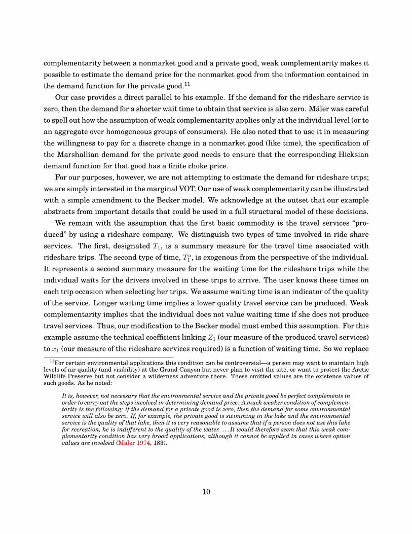
complementarity between a nonmarket good and a private good, weak complementarity makes itpossible to estimate the demand price for the nonmarket good from the information contained inthe demand function for the private good.11
Our case provides a direct parallel to his example. If the demand for the rideshare service iszero, then the demand for a shorter wait time to obtain that service is also zero. Mäler was carefulto spell out how the assumption of weak complementarity applies only at the individual level (or toan aggregate over homogeneous groups of consumers). He also noted that to use it in measuringthe willingness to pay for a discrete change in a nonmarket good (like time), the specification ofthe Marshallian demand for the private good needs to ensure that the corresponding Hicksiandemand function for that good has a finite choke price.
For our purposes, however, we are not attempting to estimate the demand for rideshare trips;we are simply interested in themarginal VOT.Our use of weak complementarity can be illustratedwith a simple amendment to the Becker model. We acknowledge at the outset that our exampleabstracts from important details that could be used in a full structural model of these decisions.
We remain with the assumption that the first basic commodity is the travel services “pro-duced” by using a rideshare company. We distinguish two types of time involved in ride shareservices. The first, designated T1, is a summary measure for the travel time associated withrideshare trips. The second type of time, T a
1 , is exogenous from the perspective of the individual.It represents a second summary measure for the waiting time for the rideshare trips while theindividual waits for the drivers involved in these trips to arrive. The user knows these times oneach trip occasion when selecting her trips. We assume waiting time is an indicator of the qualityof the service. Longer waiting time implies a lower quality travel service can be produced. Weakcomplementarity implies that the individual does not value waiting time if she does not producetravel services. Thus, our modification to the Becker model must embed this assumption. For thisexample assume the technical coefficient linking Z1 (our measure of the produced travel services)to x1 (our measure of the rideshare services required) is a function of waiting time. So we replace
11For certain environmental applications this condition can be controversial—a person may want to maintain highlevels of air quality (and visibility) at the Grand Canyon but never plan to visit the site, or want to protect the ArcticWildlife Preserve but not consider a wilderness adventure there. These omitted values are the existence values ofsuch goods. As he noted:
It is, however, not necessary that the environmental service and the private good be perfect complements inorder to carry out the steps involved in determining demand price. Amuchweaker condition of complemen-tarity is the following: if the demand for a private good is zero, then the demand for some environmentalservice will also be zero. If, for example, the private good is swimming in the lake and the environmentalservice is the quality of that lake, then it is very reasonable to assume that if a person does not use this lakefor recreation, he is indifferent to the quality of the water. . . . It would therefore seem that this weak com-plementarity condition has very broad applications, although it cannot be applied in cases where optionvalues are involved (Mäler 1974, 183).
10
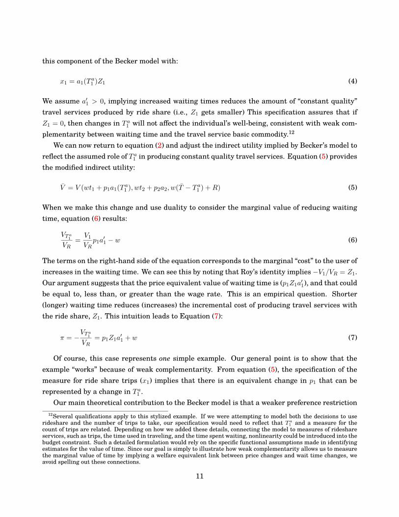
this component of the Becker model with:
x1 = a1(T a1 )Z1 (4)
We assume a′1 > 0, implying increased waiting times reduces the amount of “constant quality”travel services produced by ride share (i.e., Z1 gets smaller) This specification assures that ifZ1 = 0, then changes in T a
1 will not affect the individual’s well-being, consistent with weak com-plementarity between waiting time and the travel service basic commodity.12
We can now return to equation (2) and adjust the indirect utility implied by Becker’s model toreflect the assumed role of T a
1 in producing constant quality travel services. Equation (5) providesthe modified indirect utility:
V̄ = V (wt1 + p1a1(T a1 ), wt2 + p2a2, w(T̄ − T a
1 ) +R) (5)
When we make this change and use duality to consider the marginal value of reducing waitingtime, equation (6) results:
VT a1
VR= V1VR
p1a′1 − w (6)
The terms on the right-hand side of the equation corresponds to the marginal “cost” to the user ofincreases in the waiting time. We can see this by noting that Roy’s identity implies −V1/VR = Z1.Our argument suggests that the price equivalent value of waiting time is (p1Z1a
′1), and that could
be equal to, less than, or greater than the wage rate. This is an empirical question. Shorter(longer) waiting time reduces (increases) the incremental cost of producing travel services withthe ride share, Z1. This intuition leads to Equation (7):
π = −VT a
1
VR= p1Z1a
′1 + w (7)
Of course, this case represents one simple example. Our general point is to show that theexample “works” because of weak complementarity. From equation (5), the specification of themeasure for ride share trips (x1) implies that there is an equivalent change in p1 that can berepresented by a change in T a
1 .Our main theoretical contribution to the Becker model is that a weaker preference restriction
12Several qualifications apply to this stylized example. If we were attempting to model both the decisions to userideshare and the number of trips to take, our specification would need to reflect that T a
1 and a measure for thecount of trips are related. Depending on how we added these details, connecting the model to measures of rideshareservices, such as trips, the time used in traveling, and the time spent waiting, nonlinearity could be introduced into thebudget constraint. Such a detailed formulation would rely on the specific functional assumptions made in identifyingestimates for the value of time. Since our goal is simply to illustrate how weak complementarity allows us to measurethe marginal value of time by implying a welfare equivalent link between price changes and wait time changes, weavoid spelling out these connections.
11

than was required in Becker’s model is possible for valuing time. In the context of rideshare,we have this form of weak complementarity as people wait for the ride. An additional importantfeature of the model is the specificity of the value of time can be linked to its particular use. Thisarises in rideshare because the timing and position of rideshare trips can be linked to a widerange of purposes, tasks, and contexts, allowing for an assessment of how the properties of thesituation affect VOT measures. Taken together, we now have the theoretical machinery to valuetime through changes in prices and wait times of the good.
In this spirit, leveraging the Lyft rideshare platform, our model is specific to a trip session, inwhich a passenger opens up the app and receives a price and waiting time quote for a potentialtrip. Individual responses to the terms of a ride are indexed by passenger (i) and session (j).We assume that incomes and other prices faced by individuals opening the Lyft application arefixed across the experimental groups due to randomization, and focus our attention on the utilityrealized with and without requesting a ride. Equation (8) begins the process of formalizing thedecision associated with requesting a ride:
Vij = v(Pij , Taij) + εij (8)
Let Vij be the utility associated with selecting a Lyft ride at a price of Pij for individual i andsession j. Let Tij be the wait time indicated to individual i in session j, and εij be a random errorcapturing unobserved (to the analyst) features of the circumstances of choice.
We assume that each individual compares the realized utility from a Lyft ride with that ofa default condition that we do not observe. We assume the default option is specific to eachindividual and session and provides utility Wij . A Lyft is requested if and only if Vij > Wij . Byindependently randomizing both P and T a, we can recover estimates for the parameters used todescribe the choice process in equation (8).
The price of a Lyft ride is the product of a base price,Bij , that depends on the characteristics ofthe request (timing, route, and vehicle type) and a price multiplier (called Prime Time) (1+PTij).This multiplier is set dynamically in response to local demand and supply conditions. Bij andPTij are indexed by i and j because the records of sessions allow the timing of the session andthe individual to be distinguished.
In our case, we observe whether an individual selected a Lyft ride but cannot completely char-acterize the features of the alternative set when the ride is not chosen. This is where our assump-tion of weak complementarity provides the “traction” needed to recover a VOT. As noted earlier,when waiting time is a weak complement to the rideshare service associated with each trip, achange in wait time is equivalent, from a welfare perspective, to a change in the price of the trip(Smith and Banzhaf, 2007). The important implication is that we do not need to know anythingabout a passenger’s labor supply decisions to recover an estimate for the opportunity cost for theirtime; the price of the Lyft ride serves this role. Thus, with appropriate exogenous variation in
12

both trip prices and wait times, consumers’ actual choices allow us to identify the key thresholdtrade-offs between time and money that serve to recover the VOT.13
The decision process in our model begins with the assumption that each individual is consid-ering a “local” trip, that is within his or her metropolitan area. We observe everyone who opensthe Lyft application during our experimental period. Yet, we do not know their complete set ofoutside options, and because of this limitation we consider a variety of approaches to organizesessions to account for our hypothesized differences in how these outside alternatives influenceWij for each individual. There are several implications of this constraint on what can be observed.The first of these is the selection effect directly associated with knowing only those who open theLyft app; we discuss the implications of this external validity issue in Appendix Section H. More-over, because we cannot characterizeWij , we do not have a reference or baseline condition that wewould expect in defining a reference utility level to measure a VOT. This limitation influences ourinterpretation of the estimates. Without specifying the outside alternative, we estimate choiceprobabilities relative to a normalizing alternative.14
2.2 Empirical Model
Our primary model specification for the choice process is contained in equation (8), which com-pares Vij withWij using the log transformation for the price and wait time as determinants of theobserved trip request, Rij(0, 1). We assume that passenger i in their jth session receives greaterutility from requesting a ride, Vij , than the alternative Wij , and thus the request, Rij , is madeaccording to:
Rij = β1 lnPij + β2 lnT aij + εij = β0 lnBij + β1 ln(1 + PTij) + β2 lnT a
ij + εij (9)
Here Pij is the offered price, T aij the offered wait time for the ride, Bij is the base price, and
εij is the unobserved error term. The price of a ride is the product of a base price Bij and a pricemultiplier, (1+PTij), which is set dynamically in response to local supply and demand conditions.By using the log transformation for the price and wait time in equation (9), the choices reveal thepreference parameters needed to recover our measure for the price equivalent of waiting timewithout knowing the base price for each request.15 This formulation allows a separation of thebase price and the price multiplier as determinants of the request, and identification of the price
13We do not need to specify a global model of time use with every commodity and price in it. Weak complementaritywith random prices and wait time at the point of purchase is enough.
14In general, we do not know if a person actually considered the alternatives that were available, and only knowthat they were feasible when a decision to select a mode was made. As McFadden (1974) demonstrated, given thespecification of the factors influencing an individual’s choices and an assumed choice set, the inability to know aspecific default alternative or all the possibilities does not prevent one from assessing the relative importance of eachdeterminant using a random sample of the hypothesized alternatives, together with assumptions that characterizethe choice process. For many applications, this constraint on the information available is not important to the results.
15We considered other functional forms as robustness checks; see Table C.23 in Appendix C. We also discuss this insection 3.4.1.
13
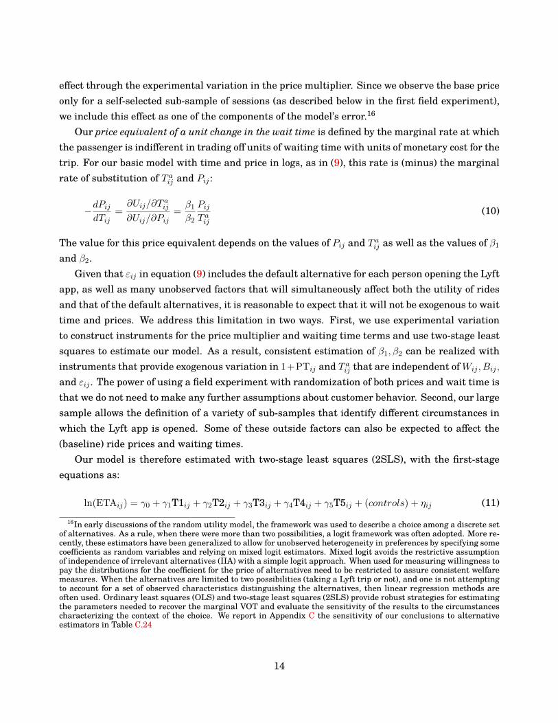
effect through the experimental variation in the price multiplier. Since we observe the base priceonly for a self-selected sub-sample of sessions (as described below in the first field experiment),we include this effect as one of the components of the model’s error.16
Our price equivalent of a unit change in the wait time is defined by the marginal rate at whichthe passenger is indifferent in trading off units of waiting time with units of monetary cost for thetrip. For our basic model with time and price in logs, as in (9), this rate is (minus) the marginalrate of substitution of T a
ij and Pij :
−dPij
dTij=∂Uij/∂T
aij
∂Uij/∂Pij= β1β2
Pij
T aij
(10)
The value for this price equivalent depends on the values of Pij and T aij as well as the values of β1
and β2.Given that εij in equation (9) includes the default alternative for each person opening the Lyft
app, as well as many unobserved factors that will simultaneously affect both the utility of ridesand that of the default alternatives, it is reasonable to expect that it will not be exogenous to waittime and prices. We address this limitation in two ways. First, we use experimental variationto construct instruments for the price multiplier and waiting time terms and use two-stage leastsquares to estimate our model. As a result, consistent estimation of β1, β2 can be realized withinstruments that provide exogenous variation in 1+PTij and T a
ij that are independent ofWij , Bij ,
and εij . The power of using a field experiment with randomization of both prices and wait time isthat we do not need to make any further assumptions about customer behavior. Second, our largesample allows the definition of a variety of sub-samples that identify different circumstances inwhich the Lyft app is opened. Some of these outside factors can also be expected to affect the(baseline) ride prices and waiting times.
Our model is therefore estimated with two-stage least squares (2SLS), with the first-stageequations as:
ln(ETAij) = γ0 + γ1T1ij + γ2T2ij + γ3T3ij + γ4T4ij + γ5T5ij + (controls) + ηij (11)16In early discussions of the random utility model, the framework was used to describe a choice among a discrete set
of alternatives. As a rule, when there were more than two possibilities, a logit framework was often adopted. More re-cently, these estimators have been generalized to allow for unobserved heterogeneity in preferences by specifying somecoefficients as random variables and relying on mixed logit estimators. Mixed logit avoids the restrictive assumptionof independence of irrelevant alternatives (IIA) with a simple logit approach. When used for measuring willingness topay the distributions for the coefficient for the price of alternatives need to be restricted to assure consistent welfaremeasures. When the alternatives are limited to two possibilities (taking a Lyft trip or not), and one is not attemptingto account for a set of observed characteristics distinguishing the alternatives, then linear regression methods areoften used. Ordinary least squares (OLS) and two-stage least squares (2SLS) provide robust strategies for estimatingthe parameters needed to recover the marginal VOT and evaluate the sensitivity of the results to the circumstancescharacterizing the context of the choice. We report in Appendix C the sensitivity of our conclusions to alternativeestimators in Table C.24
14

ln(1 + PTij) = δ0 + δ1T1it + δ2T2it + δ3T3ij + δ4T4ij + δ5T5ij + (controls) + ζij (12)
and the second-stage equation is:
Requestij = β0 + β1 ln(1 + PTij) + β2 ln(ETAij) + (controls) + εij . (13)
Here T1 through T5 are dummy indicators of the experimental treatment assignments (describedbelow), and controls include a vector of fixed effects for passenger and session types (e.g., a user’snumber of past rides with Lyft) as well as time and location, controlling for the unobserved vari-ation inWij and lnBij .
The estimated β1 and β2, as well as assumed values for Pij and ETAij , allow recovery of theprice equivalent of a unit of waiting time. We evaluate our price equivalent at the control averagewaiting time and control average price on completed rides during our experimental period. Theincremental price equivalent is estimated by:
β̂1
β̂2
P̄
T̄ a,
where P̄ and T̄ a are the average price and waiting time for control units.17
In Section 3 below, we fully describe our two field experiments to identify how agents trade offunits of waiting timewith units ofmonetary cost. Our first field experiment randomly assigns Lyftusers to a control or one of five treatments (T1 through T5 in our 2SLS model) varying (increase,decrease, or market) price and/or wait time (increase or market). Each individual remains withthe assignment they are given at the time of their first opening of the Lyft application duringour experimental time period (eight weeks). The realized values for both wait time and pricedepend upon the circumstances of the session; the Prime Time multiplier and waiting time arethus endogenous variables to the request decision. We use the features defining our treatments todefine instruments for both variables. We also add additional controls that identify the featuresof the context in which a person opens the app. We use the 2SLS approach above to estimate ourchoice equations, but also report alternative estimates in Appendix Section C.
A second, complementary, field experiment—in which only ETA increases are randomized(while prices remain at market values)—explores more fully the circumstances of choice and howthey allow us to measure heterogeneity. In particular, extra wait time is varied across location-time blocks (as opposed to across users) which provides (i) a robustness check on the results fromour first field experiment and (ii) additional insights into how users’ time elasticities may vary
17The decision to evaluate the VOT at the control average price and waiting time is somewhat arbitrary, and due tothe nonlinearity of the expression for the VOT in price and waiting time, the VOT expression evaluated at the averageprice and waiting time may differ from the average VOT.We address this concern in Appendix L by constructing a VOTestimate for each observation using observation-specific price and waiting time predictions (and semi-elasticities); thisprocess produces a full distribution of VOTs across sessions rather than a single estimate.
15
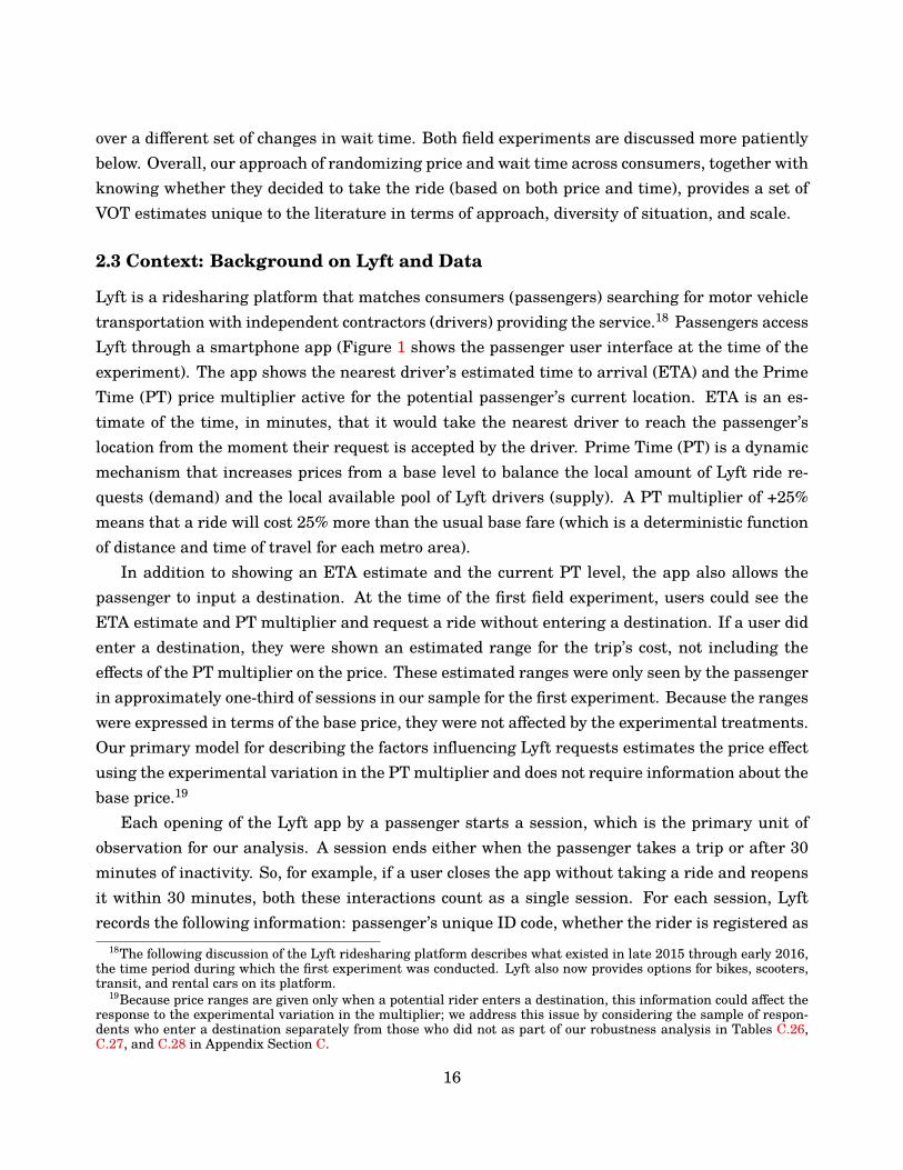
over a different set of changes in wait time. Both field experiments are discussed more patientlybelow. Overall, our approach of randomizing price and wait time across consumers, together withknowing whether they decided to take the ride (based on both price and time), provides a set ofVOT estimates unique to the literature in terms of approach, diversity of situation, and scale.
2.3 Context: Background on Lyft and Data
Lyft is a ridesharing platform that matches consumers (passengers) searching for motor vehicletransportation with independent contractors (drivers) providing the service.18 Passengers accessLyft through a smartphone app (Figure 1 shows the passenger user interface at the time of theexperiment). The app shows the nearest driver’s estimated time to arrival (ETA) and the PrimeTime (PT) price multiplier active for the potential passenger’s current location. ETA is an es-timate of the time, in minutes, that it would take the nearest driver to reach the passenger’slocation from the moment their request is accepted by the driver. Prime Time (PT) is a dynamicmechanism that increases prices from a base level to balance the local amount of Lyft ride re-quests (demand) and the local available pool of Lyft drivers (supply). A PT multiplier of +25%means that a ride will cost 25% more than the usual base fare (which is a deterministic functionof distance and time of travel for each metro area).
In addition to showing an ETA estimate and the current PT level, the app also allows thepassenger to input a destination. At the time of the first field experiment, users could see theETA estimate and PT multiplier and request a ride without entering a destination. If a user didenter a destination, they were shown an estimated range for the trip’s cost, not including theeffects of the PT multiplier on the price. These estimated ranges were only seen by the passengerin approximately one-third of sessions in our sample for the first experiment. Because the rangeswere expressed in terms of the base price, they were not affected by the experimental treatments.Our primary model for describing the factors influencing Lyft requests estimates the price effectusing the experimental variation in the PT multiplier and does not require information about thebase price.19
Each opening of the Lyft app by a passenger starts a session, which is the primary unit ofobservation for our analysis. A session ends either when the passenger takes a trip or after 30minutes of inactivity. So, for example, if a user closes the app without taking a ride and reopensit within 30 minutes, both these interactions count as a single session. For each session, Lyftrecords the following information: passenger’s unique ID code, whether the rider is registered as
18The following discussion of the Lyft ridesharing platform describes what existed in late 2015 through early 2016,the time period during which the first experiment was conducted. Lyft also now provides options for bikes, scooters,transit, and rental cars on its platform.
19Because price ranges are given only when a potential rider enters a destination, this information could affect theresponse to the experimental variation in the multiplier; we address this issue by considering the sample of respon-dents who enter a destination separately from those who did not as part of our robustness analysis in Tables C.26,C.27, and C.28 in Appendix Section C.
16
a business user, the local start time, the passenger’s current location (latitude and longitude),counts of how many requests the passenger makes and rides the passenger completes, as well asthe ETA and PT shown to the passenger in the session. ETA and PT may vary over the course ofone session due to real-time changes in local supply and demand. As such, our analysis focuseson the last shown ETA and PT in the session, as these are the ones faced by the passenger attheir final decision node of whether to request a ride.20 Thus, all of our discussion of the ETA andPT will refer to the last value presented in a session (unless otherwise specified).
From these data, we can define a number of variables to characterize the circumstances facingthe potential passengers as they made their choices. For example, using a deidentified, unique IDfor a passenger, we can determine how many Lyft rides that passenger has taken. Using sessionstart times, we can categorize a session as taking place on a weekend evening, during themorningcommute, or in any other time category. And, using location data, we can determine if a passengeris at an airport or at a downtown or suburban location for each metro area in our sample. Finally,note that Lyft offers various ride modes, including Classic (the standard mode), Lyft Line, nowcalled Shared, (inwhich several passengers share a single car withmultiple pickups and dropoffs),and Lyft XL (which offers larger vehicles). At the time of the experiment, the majority of rides(about three-quarters) were Classics. We include all ride types in our analysis, and considerexclusion of non-Classic sessions as a robustness check (see Appendix Section K).
3. Design and Results For Field Experiment 1
To identify how agents trade off time and money, we begin with a first natural field experiment(see Harrison and List (2004) for the various field experiment definitions) that randomly assignedconsumers to one of several treatments that differ in both the realized wait time and price (i.e.Field Experiment 1). The second natural field experiment, which we denote as Field Experiment2, is described in Section 4.
3.1 Design of Field Experiment 1
The process that determines both the price multiplier and the waiting time implies that bothvariables are endogenous. The PT algorithm is designed to raise prices during periods of relativehigh demand/low supply; similarly, the number of available drivers at the time each potentialrider opens the app in relation to the others who do so at the same time in a location will de-termine the estimated wait time. Our first field experiment involved nine cities in the U.S. (SanFrancisco, Austin, Atlanta, Miami, Los Angeles, San Diego, Boston, Seattle, and New York City)
20ETAs vary over the course of a session in 51.3% of sessions, while PT varies in 11.9% of sessions. The intra-sessionvariation in ETAs is caused by drivers continuously moving during the course of a session, and is generally small. Forexample, in 76.4% of sessions, the difference between the maximum and minimum ETAs shown is one minute or less.
17
for eight weeks between December 2015 and January 2016, which involved 720,059 customersand 5,177,358 individual sessions.21
At the start of the experiment, 37% of all users in each city were randomly assigned to a controlor one of five treatment groups. The experimental treatments ensure that there is exogenousvariation in the components of each algorithm determining the PT multiplier and the wait time.The algorithm for wait time can increase the wait time above the normal arrival time, but cannotreduce the wait time. As a result, the wait time variations are limited to a high and normal(ETA). Each is matched with three possible treatments for the price algorithm: low, normal, andhigh. The sub-sample assigned to the normal ETA and normal price combination is treated asthe control group. The remaining 63% of users associated with other sessions are excluded fromour main analysis.22
The proportion of users randomly assigned to each group is shown in Table 1.23 Table C.1compares the features of the control and the treatment groups in terms of the available variablesfor describing each session. Based on these variables, the randomization achieved balance on theobservable covariates.
Throughout the eight weeks of the experiment, each individual remained in the same treat-ment. Thus, a user assigned to the low price, high ETA treatment group had all of his or hersessions during the eight weeks subjected to the same algorithm, which would lead to potentiallylower price and higher waiting times than what would be the case if they were in the controlgroup. Of course, in practice, specific values for the wait time and price multiplier vary depend-ing on how local conditions affected the outcomes produced by each algorithm. We understandthe potential selection effects that might occur from this long-term design (although we use a dif-ferent design in the second field experiment), and we analyze such effects thoroughly in AppendixSection I.
Price variation was achieved by modifying each user’s PT multiplier, increasing it (for highprice treatment groups) or decreasing it (for low price treatment groups) based on local marketimbalances. This modification has the effect of raising or lowering a user’s effective price, butnot necessarily in every session.24 Waiting time variation was achieved by removing drivers fromthe nearest driver queue of each affected passenger: the nearest driver, all drivers whose ETA
21Sessions in one city, Nashville, were dropped due to implementation problems with the experimental treatments.Including Nashville data in our full-sample regressions does not significantly change our point estimates. See FigureB.3 for the number of sessions per day over the full duration of the experiment (eight weeks).
22These sessions were not used as additional control observations because they may have been subject to otherexperiments conducted at Lyft concurrently with our field experiment.
23Treatment group assignments are determined by applying a hash function to each user’s unique Lyft ID code.Since the assignment of each user to a treatment was random, we can assume that users in each treatment group area representative sample of ride share users who open the Lyft app in the affected cities during the time of the firstexperiment.
24More concretely, because PT takes values in a fixed, discrete set (0%, 25%, 50%, etc.), the change in the algorithm’ssensitivity to market conditions may not always result in a different PT level. For example, if the market has muchmore supply than demand, both the normal and the more sensitive, high price algorithm may find that the optimalPT level in the allowed set is 0%.
18
was within 30 seconds of that of the nearest driver, and one additional driver were removedfrom the queue. This removal has the effect of increasing ETA by at least 30 seconds for allpassengers subject to the high ETA treatment, but potentially by considerably more than 30seconds, especially when there are few drivers near a passenger. Because each passenger’s priceand ETA treatments are independent, we can identify the coefficients for both price and timeeffects on the demand for Lyft rides.
Table 2 displays average ETA, PT, and completed ride price by treatment group. The random-ization was successful: our high ETA treatment increases the ETAs by an average of approxi-mately 1.6 minutes, an increase of about 52%. The high price treatment increases average PTlevels from about 10.0% to 16.3%, while the low price treatment decreases the average PT levelsto about 3.6%. These PT differences result in completed ride prices that are about 2.5% higherfor passengers receiving high price treatments and 2.0% lower for passengers receiving low pricetreatments.25
Table C.5 and Figures 2 and 3 show the distributions of PT and ETAs for each of the sixtreatment groups.26 Appendix B provides graphs of the distributions for each variable, indicatingthat each of the treatments shifts the distributions in the intended directions. Tables C.3 andC.4 in the Appendix report p-values from Kolmogorov-Smirnov tests of the hypotheses that thedistributions of average ETA and PT across users differs between treatment groups; the resultssuggest that the ETA distributions are approximately identical across PT treatments and viceversa, consistent with the independence of these components of the experimental treatments.27
3.2 Results of Field Experiment 1
3.2.1 Summary Statistics
Lyft customers in the experiment had, on average, about seven sessions and about four sessionswith a completed ride (see Table C.2). Customers in the high ETA and high price treatments hadfewer sessions, ride requests, and completed rides than control passengers, while passengers inthe normal ETA, low price treatment group had slightly more than the control. These differencesare consistent with a treatment effect on passenger behavior, which we explore further below.28
Before moving to the formal analysis, we consider the effects of the various treatments on pas-sengers’ demand behavior. The lower panel in Table C.2 shows the average number of sessions
25The effects of treatment on completed ride price are smaller than the effects on quoted PT because PT itself affectsthe probability that a session will result in a completed ride.
26Two sessions had recorded ETAs of 0 minutes. These were dropped from the data, so that the log transformationcould be applied to ETA.
27Figures B.1 and B.2 in the Appendix indicate that these treatments are in effect consistently throughout the courseof the experiment.
28Figures B.7, B.8, B.9, and B.10 highlight the heterogeneity in our sample. While the majority of our sessionscome from San Francisco and Los Angeles, we have a large number of observations from the other six cities in theexperiment. The distributions of sessions over days of the week and hours of the day are relatively balanced, thoughweekend and late afternoon/early evening times are the best represented time periods in our sample.
19
which had ride requests for each treatment group. Figures 4 and B.11 display the demand rate,defined in two ways. The first, Figure 4, uses the total requests for service compared to thoseopening the Lyft app. The second definition uses completed rides in place of requests. Somerequests are not completed because a passenger is not matched to a driver, or the passenger ordriver cancels a ride before it is finalized. These situations amount to 0.6% and 10.0% of the totalrequests during experiment 1, respectively.29 As expected, the high ETA and price treatmentsdecrease request rates relative to the control, while the low price treatment increases requestrates. The small confidence intervals around the means suggest that these differences are statis-tically significant at the 95% level, and the magnitude of the differences of request rate betweentreatment groups—which is as large as four percentage points between the normal ETA, low pricetreatment and the high ETA, high price treatment suggest the outcomes reflect economically con-sistent responses to the differences in the circumstances of choice. For example, the high ETA,low price treatment had a slightly higher request rate than control, and the high ETA, normalprice treatment had a slightly higher request rate than the normal ETA, high price treatment.30
3.2.2 Empirical Estimation
Our dependent variable is a discrete indicator for a request for the service (1 for request, 0 oth-erwise) with ln(ETA) and ln(1 + PT) as the independent variables of direct interest. We alsohave a set of controls that include fixed effects for the location, local hour of week and week ofyear, user experience with Lyft (decile of pre-experiment lifetime rides), and user type (whetherthe use has a business profile). Since the data generating process implies ETA and PT will beendogenous, 2SLS is our preferred estimator. As part of a robustness analysis, we estimated aprobit model (instrumenting ln(ETA) and ln(1 + PT)) of our main specification and report theseresults in Table C.24 in Appendix C. Standard errors are estimated clustering within passengers
29Figure B.4 in the Appendix considers how the average number of rides a passenger in each treatment group takesevolves over the course of the experiment, relative to the average number of rides a control passenger takes. The fiveseries are approximately comparable at the outset of the experiment, appear to spread out with the duration of theexperiment, and then appear to stabilize about 10 days after a user’s first session in the experiment.Figure B.5 in the Appendix is a similar plot comparing session rates (that is, percentage of passengers opening
the app) between the treatment groups over time. Expected effects of the treatments on rates of use of the platformare observed: passengers facing the higher prices and waiting times become less likely to return to the platform overtime. Price and waiting time thus have both intensive- and extensive-margin effects on demand, impacting not onlythe passenger’s probability of requesting after opening the app, but also the probability that the passenger opens theapp again in the future. We explore how this extensive margin behavior impacts the VOT estimation in section 3.4.
Finally, our observations are distributed evenly over passenger/experience levels. That is, we observe a near equalnumber of sessions for passengers with 0 rides and over 50 rides before the start of the experiment. The presence ofthis heterogeneity across regions, time, and passengers allows us to investigate how the value of time varies acrosscircumstances.
30In addition to these during-experiment demand effects, we also find some evidence of treatment effects persistingbeyond the end of the experiment; see Appendix E.
20
and are assumed independent across passengers.31
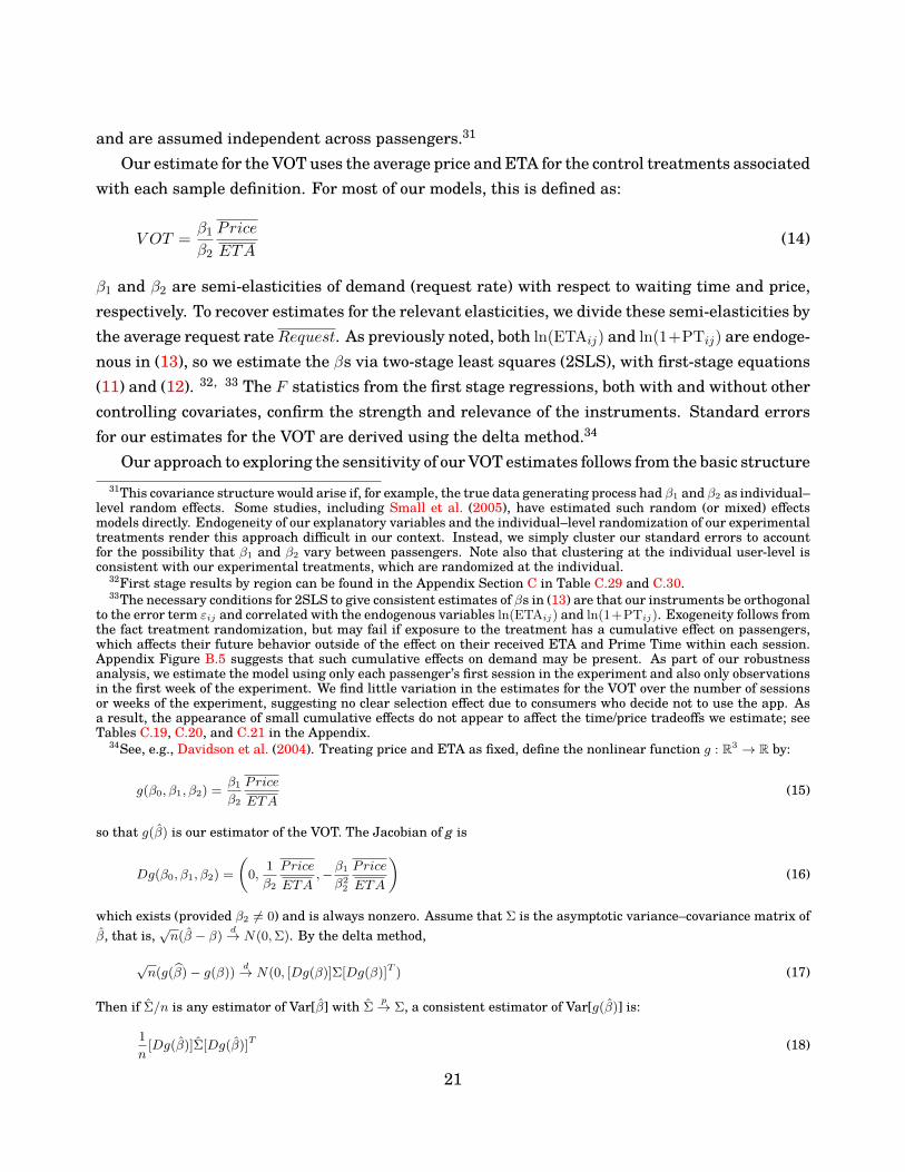
Our estimate for the VOT uses the average price and ETA for the control treatments associatedwith each sample definition. For most of our models, this is defined as:
V OT = β1β2
Price
ETA(14)
β1 and β2 are semi-elasticities of demand (request rate) with respect to waiting time and price,respectively. To recover estimates for the relevant elasticities, we divide these semi-elasticities bythe average request rateRequest. As previously noted, both ln(ETAij) and ln(1+PTij) are endoge-nous in (13), so we estimate the βs via two-stage least squares (2SLS), with first-stage equations(11) and (12). 32, 33 The F statistics from the first stage regressions, both with and without othercontrolling covariates, confirm the strength and relevance of the instruments. Standard errorsfor our estimates for the VOT are derived using the delta method.34
Our approach to exploring the sensitivity of our VOT estimates follows from the basic structure31This covariance structure would arise if, for example, the true data generating process had β1 and β2 as individual–
level random effects. Some studies, including Small et al. (2005), have estimated such random (or mixed) effectsmodels directly. Endogeneity of our explanatory variables and the individual–level randomization of our experimentaltreatments render this approach difficult in our context. Instead, we simply cluster our standard errors to accountfor the possibility that β1 and β2 vary between passengers. Note also that clustering at the individual user-level isconsistent with our experimental treatments, which are randomized at the individual.
32First stage results by region can be found in the Appendix Section C in Table C.29 and C.30.33The necessary conditions for 2SLS to give consistent estimates of βs in (13) are that our instruments be orthogonal
to the error term εij and correlated with the endogenous variables ln(ETAij) and ln(1+PTij). Exogeneity follows fromthe fact treatment randomization, but may fail if exposure to the treatment has a cumulative effect on passengers,which affects their future behavior outside of the effect on their received ETA and Prime Time within each session.Appendix Figure B.5 suggests that such cumulative effects on demand may be present. As part of our robustnessanalysis, we estimate the model using only each passenger’s first session in the experiment and also only observationsin the first week of the experiment. We find little variation in the estimates for the VOT over the number of sessionsor weeks of the experiment, suggesting no clear selection effect due to consumers who decide not to use the app. Asa result, the appearance of small cumulative effects do not appear to affect the time/price tradeoffs we estimate; seeTables C.19, C.20, and C.21 in the Appendix.
34See, e.g., Davidson et al. (2004). Treating price and ETA as fixed, define the nonlinear function g : R3 → R by:
g(β0, β1, β2) = β1
β2
Price
ETA(15)
so that g(β̂) is our estimator of the VOT. The Jacobian of g is
Dg(β0, β1, β2) =(
0, 1β2
Price
ETA,−β1
β22
Price
ETA
)(16)
which exists (provided β2 6= 0) and is always nonzero. Assume that Σ is the asymptotic variance–covariance matrix ofβ̂, that is, √n(β̂ − β) d→ N(0,Σ). By the delta method,
√n(g(β̂)− g(β)) d→ N(0, [Dg(β)]Σ[Dg(β)]T ) (17)
Then if Σ̂/n is any estimator of Var[β̂] with Σ̂ p→ Σ, a consistent estimator of Var[g(β̂)] is:
1n
[Dg(β̂)]Σ̂[Dg(β̂)]T (18)
21
of the Becker model. The first of these is the selection of functional form describing how wait timeand price influence requests. By transforming the price and time using logs we can estimate theparameter describing how people respond to price knowing only the PT multiplier. Second, torecover ameasure of the VOTwe need to select a point for evaluating the implied time/price trade-off. As noted earlier, we use the average values for these variables from the control treatmentsto estimate the semi-elasticities. Finally, to develop insights into how the circumstances of eachperson’s choice affect the VOT, we estimate the VOT using a set of sub-samples motivated by anextension of the Becker theory, which is presented below.
3.2.3 VOT Estimates
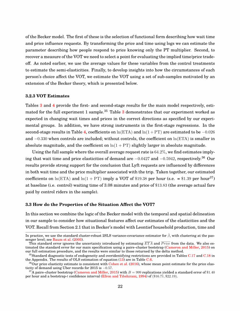
Tables 3 and 4 provide the first- and second-stage results for the main model respectively, esti-mated for the full experiment 1 sample.35 Table 3 demonstrates that our experiment worked asexpected in changing wait times and prices in the correct directions as specified by our experi-mental groups. In addition, we have strong instruments in the first-stage regressions. In thesecond-stage results in Table 4, coefficients on ln(ETA) and ln(1 + PT) are estimated to be −0.026and −0.330 when controls are included; without controls, the coefficient on ln(ETA) is smaller inabsolute magnitude, and the coefficient on ln(1 + PT) slightly larger in absolute magnitude.
Using the full sample where the overall average request rate is 64.2%, we find estimates imply-ing that wait time and price elasticities of demand are −0.0427 and −0.5942, respectively.36 Ourresults provide strong support for the conclusion that Lyft requests are influenced by differencesin both wait time and the price multiplier associated with the trip. Taken together, our estimatedcoefficients on ln(ETA) and ln(1 + PT) imply a VOT of $19.38 per hour (s.e. = $1.39 per hour37)at baseline (i.e. control) waiting time of 3.08 minutes and price of $13.83 (the average actual farepaid by control riders in the sample).
3.3 How do the Properties of the Situation Affect the VOT?
In this section we combine the logic of the Becker model with the temporal and spatial delineationin our sample to consider how situational features affect our estimates of the elasticities and theVOT. Recall from Section 2.1 that in Becker’s model with Leontief household production, time and
In practice, we use the standard cluster-robust 2SLS variance-covariance estimator for β̂, with clustering at the pas-senger level; see Baum et al. (2003).
This standard error ignores the uncertainty introduced by estimating ETA and Price from the data. We also es-timated the standard error for our main specification using a pairs–cluster bootstrap (Cameron and Miller, 2015) onour full estimation procedure, and the results were similar to those returned by the delta method.
35Standard diagnostic tests of endogeneity and overidentifying restrictions are provided in Tables C.17 and C.18 inthe Appendix. The results of OLS estimation of equation (13) are in Table C.6.
36Our price elasticity estimate is consistent with Cohen et al. (2016), whose mean point estimate for the price elas-ticity of demand using Uber records for 2015 is −0.57.
37A pairs–cluster bootstrap (Cameron and Miller, 2015) with B = 999 replications yielded a standard error of $1.40per hour and a bootstrap-t confidence interval (Efron and Tibshirani, 1994) of ($16.71, $22.19).
22

private goods are perfect complements. When this restriction is relaxed, the wait time and priceof a rideshare trip enter the indirect utility function without restriction, and we may considerhow each of these influences our measure of the value of time.
Consider the willingness to pay WTP for a price increase (1 + PT0 to 1 + PT1) and waitingtime decrease (ETA0 to ETA1). W is defined by equation (19).
V (1 + PT1, ETA1,m−WTP ) = V (1 + PT0, ETA0,m) (19)
Denoting the marginal value of time (VET A/Vm) by π and the demand for rideshare trips by T , wehave the following second-order expansion forWTP :
WTP ≈ π(ETA1 − ETA0)− T (PT1 − PT0) + 12(πET A − ππm)(ETA1 − ETA0)2
− 12(TP T + TTm)(PT1 − PT0)2 + (πP T + Tπm)(ETA1 − ETA0)(PT1 − PT0).
(20)
When the changes in price and waiting time exactly offset each other, we have WTP = 0. Ifwe also assume that T = 1 and that the adjustment of trips to price (TP T ) and income (Tm) areneglible, we can solve for the ratio of the price change to the equivalent waiting time change:
PT1 − PT0ETA1 − ETA0
≈ π + 12(πET A − ππm)(ETA1 − ETA0) + (πP T + πm)(PT1 − PT0). (21)
Equation (21) shows that, to first order, the ratio of the price change to the equivalent waiting timechange equals the value of time π. The equation further shows that this ratio is also influencedby the size of the waiting time change (ETA1 − ETA0), the sensitivity of the VOT to the waitingtime (πET A), and the sensitivity of the VOT to income (πm).
This conventional model fails to capture another of Becker’s insights: the context of choice.The simple Leontief version of his model captured this effect by allowing time to be linked indifferent ways to different private goods. We observe only one private service: rideshare trips.Nonetheless, we can observe how the price equivalent changes in different situations, indexedby location, time of day, and weather condition. This rich detail in the circumstances of people’schoices allows the data to add resolution to what a largely unrestricted model may imply forthe VOT. By selecting sub-samples distinguished by the location, timing, and other features ofpassenger sessions, we can evaluate how each affects potential users’ decisions with randomlyvaried prices and wait times, yielding heterogeneity tests across three bins of the data:
1. Individual trip features that are correlated with the opportunity cost of time, which in-clude purpose of trip, time and day of week of trip, and specific location of trip. Such mone-tary values are driven by what activities are crowded out by greater wait times.
2. Other trip signatures such as weather conditions, the baseline ETA, and who bears the23

marginal cost of the trip. In this case, when the cost burden is shared by an employer therider should be more sensitive to temporal changes.
3. Market variables that are correlated with the opportunity cost of time, which include localwages and the available substitutes, such as access to alternative public transportation.Such variables affect the nature and shape of the demand curve for time.
Taken together, data generated across both natural field experiments combine to shed im-portant insights on factors within each bin. In each bin, a mixture of experimental and non-experimental variation is utilized, and we take caution in interpreting results based on thenaturally-occurring variation and selection below. The features which define each bin may becorrelated with other features affecting preferences and the circumstance of choice; in AppendixJ we attempt to address this concern in a secondary experiment by reweighting observationswithin each bin to balance the distributions of other relevant observable covariates.38
3.3.1 Individual Trip Features
Table 5 summarizes our findings concerning trip and market features.39 Consider first the differ-ent ways of describing the timing for choices: by day of the week and by an hour of the day. In thelatter case, we also distinguish weekends (Saturday and Sunday) from weekdays. Our reasoningabove yields predictions on how the various situations should affect VOT estimates. More specif-ically, in the case of distinguishing days of the week we would expect that the opportunity cost oftime is higher during weekdays than on weekends. Our estimates in Table 5 support this conclu-sion, as weekdays experience ETA elasticities larger than we observe on weekends. And, VOTsaverage nearly $20 during the week versus around $18 on the weekend. While these differencesare meaningful, overall they are not consistently different at conventional significance levels.
Yet, when we consider the time of the day, distinguishing weekdays from weekends, we findpronounced and statistically significant differences in the VOT estimates at the p < 0.01 level.These differences mainly arise in the morning and evening commuting rush hour periods forweekdays (6 to 10 AM and 4 to 7 PM) where we observe larger ETA elasticities (especially in themornings) and higher VOTs—averaging above $24—compared to non-commuting time blocks.For weekends, we observe less variation throughout the day, as we might expect.
These estimates suggest that when the wait time crowds out work time the ETA elasticityand the VOT estimates are higher than when it crowds out non-work time. In this manner, the
38We also indirectly examine the impact of reliability by checking the robustness of our results when we includecontrols for late arrivals in passengers’ previous interactions with the Lyft app in Appendix Section D. Similarly, weattempt to address the potential bias that may arise from not accounting for the effect of in-vehicle time on passengerdemand in Appendix Section F. Finally, we check the sensitivity of our results to the presence of always- or never-requesters in our sample in Appendix Section G, and to user selection in Appendix Section I.
39The corresponding full regression tables are C.7 and C.8 in the Appendix.
24

pattern of results observed in Table 5 are consonant with the notion that individual trip featurespredictably affect the relevant primitives in the model.40
3.3.2 Other Trip Characteristics
Table 6 considers other features of the trip that potentially affect the marginal sensitivities toprice and waiting time.41 Our data from this first field experiment allows us to distinguish choicesalong the dimension of wait time unpleasantries as well as who bears the burden of the trip. Fieldexperiment 2 provides the necessary variation to explore how baseline ETA variation impactsVOT estimates and therefore provides a sense of the curvature of the VOT. We discuss thoseresults in Section 4.
The top panel of Table 6 provides our full sample estimates, and as a comparison the middlepanel provides relevant estimates when there is rain, snow, and no precipitation.42 We find thatthe trips with adverse weather conditions suggest a clear and discernible impact on the VOTestimates, suggesting that precipitation makes longer waiting times considerably less desirable.For instance, in the presence of snow, the ETA elasticity is more than two times higher thanwhen there is no precipitation. This enhanced time sensitivity leads the VOT estimate to benearly 40% higher than no precipitation trips ($26.56 versus $19.04). The effect of rain, whilemuted compared to snow, is also significantly larger than when there is no precipitation.
While both rain and snow cause the ETA elasticities to be higher, and in turn increasingthe VOT estimates, tempering these increases are the price elasticity increases that we observe.While such increases are indeed small, we expected that as weather conditions worsen consumerswould become less sensitive to price changes. These estimates may reflect that baseline PT ishigher in such cases (15.2% in rain and 20.0% in snow).
The bottom panel of Table 6 provides insights into how the burden of cost affects the relevantelasticities. We use information on whether the trip was taken by a business or a non-businessuser, and make the assumption that the cost burden is lower for the former either because theirfirm pays the expense or if that is not the case at least the expense can be used a tax write-off. Inboth cases, the consumer bears less than 100% of the cost of trip burden.
We find that business users’ ETA elasticities andVOTs are different from those of non-businessusers in expected ways: non-business users have a price elasticity that is roughly 50% larger (-0.605 versus -0.399), and a value of time about 25% higher. Inspecting the relevant elasticities,we note that this difference is driven by business users showing much less sensitivity to price,presumably reflecting the fact that business users may not themselves bear the full monetary
40In Appendix I, we find that these heterogeneity results are robust to correcting for user selection into differenttrip contexts.
41The corresponding full regression tables are C.9 and C.10 in the Appendix.42We obtain historical realized weather data from Dark Sky at the geohash4-hour level, and match this information
to sessions based on the passenger’s geohash4 and the starting hour of the session.
25
cost of a trip.43
3.3.3 Market Factors
Results on the effects of market factors on the VOT are summarized in Table 7.44 We distinguishchoices by location in three ways: by metro area; by prominent locations within each metro area(airports and downtown locations); and by distance to the nearest public transport station/stop.45
Point estimates of the VOT vary between metro areas, but we fall short of rejecting the null ofhomogeneity across regions (p = 0.154).46 While the estimates for Atlanta, Austin, and Seattle aredistinctive, with the VOT for the first two metro areas smaller than our overall sample estimate,only the results for Atlanta would be judged as having a marginally significant difference fromthe estimate for the rest of the sample. We discuss more of the city-level estimates with respectto wages in Section 5.1.
Distinguishing downtown locations, the estimates indicate a greater VOT for downtown lo-cations compared to non-downtown.47 Trips initiating at airports have numerically larger VOTestimates, but the small sample size for these cases prevent judgement of statistical significance.The grouping of trips based on distance to nearest public transit stop yields VOT estimates thatdecrease with distance, consistent with available substitute reasoning. However, this categoryis also likely to serve as a proxy for non-downtown locations, which have lower VOT estimates.48
In the second experiment below (section 4.2.1), we have random variation in wait time that iscompletely orthogonal to the base ETA.
4. Design and Results for Field Experiment 2
4.1 Design of Field Experiment 2
Our analysis of the second natural field experiment has three primary goals: (1) replicate themain insights gained from the first field experiment on ETA elasticities and various heterogeneitytests; (2) assess the robustness of the observed heterogeneity to sample reweighting adjustments;and (3) explore how the base level of wait time affects ETA elasticities and how exogenous changes
43We are unable to assess the robustness of precipitation and business/non-business results to user selection intocontexts because our weather data does not extend far past the beginning of the first experiment and business statusdoes not vary within user.
44The corresponding full regression tables are C.11, C.12, C.13, and C.14 in the Appendix.45Public transit stop/station locations are taken from the National Transit Map, and distance is calculated as the
great circle distance between a passenger’s location and a stop.46When considering the marginal demand effects of price and waiting time separately, we do reject the nulls that
time (p = 0.046) and price (p < 0.0001) semi-elasticies are homogeneous across regions.47Maps of the areas tagged as “downtown” can be found in Figure B.6.48Results in Appendix I suggest that the distance to transit results are not primarily driven by user selection, while
the downtown/non-downtown and airport/non-airport may be. We are unable to effectively control for selection intoregions due to limited within-user variation in region (only 19% of users have a pre-experiment session in more thanone region. Full tables of regression results are available in Appendix C.
26
in the length of wait time affect the VOT. That is, by precisely varying wait time at the pickuplocation and hour (as opposed to across users in Field Experiment 1), we develop insights into howthe timing of different wait times along with their location affects time elasticities. To do thesechores, we randomized location-hour blocks into one of the following four groups: (1) Control (10%of the city sample); (2) ETA plus at least 60 seconds (5%); (3) ETA plus at least 150 seconds (3%);and (4) ETA plus at least 240 seconds (2%). To increase ETAs, we removed the closest driversfrom the dispatch queue until the ETA was increased by at least the treatment amount.
The experiment took place for eight weeks from April 2017 to June 2017 in Los Angeles, SanFrancisco, New York City, Chicago, New Jersey, Boston, Philadelphia, Washington, D.C., Miami,and Atlanta, involving 3.3 million passengers and 9.7 million sessions (5.9 million of which hadrequests for service). The randomization used in this second experiment differs from that of ourfirst experiment in that treatments were assigned at the pickup location-hour level across thewhole eight-week period. Twenty percent of all location-hour blocks in these cities in this eightweek period were in the experiment.49 Price multipliers were not randomized in this experiment;consequently, our focus is on waiting time elasticities rather than VOT estimates. Figures 5and 6 and Table C.32 show that the experimental conditions and the treatment groups have theexpected variation and overall effects on demand.50
4.2 Results of Field Experiment 2
To summarize the insights gained from our second field experiment, we split our results intotwo groups. First, we summarize the overall time elasticity estimates from field experiment 2,and explore how the properties of the situation affect the estimated ETA elasticity. In doingso, we explore how well results from field experiment 2 map into those from field experiment 1.Second, we delve into the shape of the estimated time elasticities. Section 5 focuses on the policyimplications of our results from the combination of both field experiments, digging deeper intothe relationship between VOT and local wages as well as exploring how our preferred estimatesrelate to preferred VOT values used by policymakers.
49The location unit used for this randomization is a geohash7, which has a width and height of at most 153 meters.Counts of geohash7s per region can be found in Table C.31. In all the analysis of data from this experiment, standarderrors are clustered at the geohash7-hour level, to match the clustering of the randomization scheme.
50Figures B.12 and B.13 show the timeline of the ETAs and PT respectively over the course of the experiment. It isclear that both the ETAs and PT remain pretty stable over time apart from the holiday season, especially New YearsEve where both prices and ETA increase dramatically.
27

4.2.1 Time elasticities and how they vary: a replication
The first column of Table 8 provides estimates of the time elasticity from field experiment 2. Asshown in the top row of Table 8, the estimated ETA elasticity for the full sample is −0.043.51 Thisaggregate estimate is quite close to the ETA elasticity estimate from field experiment 1; indeed,we fail to reject the homogeneity null at the p < 0.05 level for these two estimates. When we focuson data drawn from the roughly 200,000 customers who are involved in both field experiments,the estimates are also statistically indistinguishable: we fail to reject the homogeneity null at the5% level.52
The remaining estimates in column 1 of Table 8 explore heterogeneity in ETA elasticities alongdays and various times of the week. Concerning such trip features that affect the opportunitycost of time, we find qualitatively similar patterns in the ETA elasticities as we found in the firstexperiment: weekdays have larger time elasticities than weekends, and weekday elasticities arelargest during peak commuting times. Similar to experiment 1, these results show the increasedimportance of time when it relates to opportunity cost during commute hours versus other hours.
Column 2 in Table 8 shows how the ETA elasticities vary with other trip characteristics suchas inclement weather and business users. In this case, we again find that time elasticities arehigher in rainy conditions: -0.047 versus -0.042 when there is no precipitation.53 In this case,we find that business users exhibit a larger time elasticity than non-business users (−0.049 vs.−0.043) at the p < 0.01 level, despite facing lower ETAs on average (see Table C.40).
In column 3 of Table 8, we show how ETA elasticities vary spatially. Consistent with our find-ings in experiment 1, we find differences across cities in our sample, with New York and Wash-ington, D.C. having the largest elasticities (−0.086 and −0.054) and Miami and San Franciscohaving the lowest elasticities (−0.021 and −0.031). Furthermore, non-downtown sessions have alarger time elasticity than downtown sessions (−0.048 vs. −0.039) at the p < 0.01 level, though theaverage ETA is higher in the non-downtown sessions than the downtown sessions (Table C.42).
Finally, we again find that distance to public transit matters: the largest ETA elasticities areobserved for passengers more than 800 meters from their nearest public transit stop. This resultruns counter to economic intuition: passengers with better outside transportation options shouldrespond more elastically to higher waiting times. Distance to transit, however, is correlated withother relevant characteristics of the trip, such as base ETA (Table C.43). In Appendix J, we
51In these regressions, we include ln(1 + PT) as a control variable for consistency with the model used for thefirst experiment, though it is endogenous to the decision to request. Our estimates of time semi-elasticities replaceETA with an instrument constructed as predictions from a first stage regression including the treatment indicatrosand and fixed effect controls for region, geohash5, local hour of week, local week of year, business user, and decile ofuser lifetime rides (see Table C.33). These controls are also included in the second stage equation for Lyft requests.Consistency of the estimates for our time semi-elasticity relies on the exogenous treatment effects and the commoncontrols included in both the first and second stage equations. The endogenous price multiplier will not be correlatedwith our experimental variation in the ETAs each user faces, and as a result will not affect the consistency of our ETAsemi-elasticity of demand estimate. The ETA treatments do not affect ln(1 + PT), as we show in Table C.34.
52These results can be found in table C.35.53The second experiment had no sessions for which the reported precipitation type was snow.
28

adjust for these differences in the distribution of other covariates through sample weighting, andfind that the ETA elasticity is largest for passenger near public transit, as expected from thetheoretical model (Table J.6).54
4.2.2 The shape of time elasticities
An important feature of the second experiment is that we have the ability to observe multiplelevels of experimental ETA increases. As a result, we can estimate the elasticities and VOTsimplied by different increases in the wait times and can gauge the implied nonlinearity in therelationship, independent of the base wait time.
To operationalize our approach, we consider that our four levels of ETA in the field experimentprovide the ability to contrast three levels of wait time, each of which may serve as an instrumentto estimate the ETA elasticity of demand at different points of the demand curve. We considerthree sub-samples of our data: all Control and Plus 60 sessions, all Control and Plus 150 ses-sions, and all Control and Plus 240 sessions. In each sub-sample, we estimate our main demandequation, using the indicator of treatment (respectively Plus 60, Plus 150, and Plus 240) as asingle instrument for ln(ETA). The resulting coefficient estimate is a weighted average of theexpected derivative of demand with respect to ln(ETA) over the ETAs between the two treatmentlevels in the sub-sample (Angrist et al., 2000). We divide this quantity by the average requestrate in the sub-sample to obtain an estimate of the ETA elasticity of demand over the ETAs ineach sub-sample. As ETAs increase from one sub-sample to the next, comparing these elasticitiesgives insight into how the ETA elasticity of demand responds to increases in ETA.
Table 9 and 10 provide empirical results of this analysis. Overall, across every base ETA levelwe find that increasing the wait time reduces demand. This finding represents a good rationalitytest. In addition, we find that time elasticities are increasing in base ETA: at a one minute baseETA, the elasticity ranges between −0.005 and −0.018, whereas at a ten minute base ETA theelasticity ranges between −0.230 and −0.289.
The interpretation of the elasticity of−0.026 in the first row and third column of 9, for example,is that toward the lower end of the demand curve with a 3 minute base ETA, a 1% waiting timeincrease translates to a 0.026% decrease in the quantity demanded. As we can see in the secondrow, a 1% increase in ETA up to the middle portion of the demand curve reduces demand by0.044%, and the third row shows that a 1% increase in ETA up to the upper end of the demandcurve reduces demand by 0.066%. This pattern suggests that time elasticities increase as wemove further above the base waiting time.
We find that this result is consistent at all but one base ETA between one and ten minutes;time elasticities are larger for larger increases (see Table 9). In Table 11, we also find that this
54In experiment 1, we find that correcting for user selection into different distance bins does not significantly affectour ETA elasticity estimates; see Table I.5.
29
finding holds across all cities in our sample. We also find that ETA elasticities are increasingin ETA: (i) in both downtown and non-downtown sessions (Table C.46); (ii) across all days of theweek (Table C.47); and (iii) across all hours of the day (Table C.48 for weekdays and Table C.49for weekends).
There could be many mechanisms underlying the observed shape of the estimated time elas-ticities, but we are unaware of any previous causal evidence that shows themarginal value of timevaries dramatically over base wait time. Nevertheless, one concern in interpreting our analysis onthe shape of the time elasticity is that consumers’ responses may reflect a belief that a longer ETAimplies greater congestion, and then erroneously expect that their travel time would be longerthan what was stated on the app. Under this interpretation consumers might be responding tothe changes in the expected ETD in addition to changes in ETA.
We believe that this interpretation is not supported by the structure of the experiment. First, ifETA increases by one minute on the app, then the ETD is also updated by one minute, to reflectthe increase in pickup time. Second, it seems unreasonable to expect that consumers believethe quoted ETA but not the quoted ETD. Third, the consumer might believe that as time movesfurther away from the present, predictions become less accurate, and as a result the variance inETD increases. We lack the necessary data to seriously investigate such an effect, but leave thequestion open for future research.55
5 Issues in identification and external validity of our estimates
We next discuss potential threats to the internal and external validity of our natural field ex-periments. We focus on functional form assumptions (section 5.1), app competition (section 5.2),endogenous opening up of the app (section 5.3), experimental contamination (section 5.4), andexternal validity of our experimental results (section 5.5).
5.1 Functional form and specification
Our main econometric specification has wait time entering the demand equation in logarithmicform. This functional form assumption implies diminishing marginal cost of wait time. We assessthe robustness of this assumption in Tables C.23 and C.25 by running our main regressions withETA entering in levels, and find slightly larger VOTs (but not at conventional significance levels).The first experiment involves only a binary ETA treatment which does not precisely pin down anexact ETA increase (in sparse markets, for example, the treatment may induce larger absoluteETA increases than in dense markets); as a result, the experimental data provide no empiricalbasis for deciding between different functional forms. The second experiment randomizes sessions
55Table F.1 suggests that, in the 2017 experiment, ETA elasticities do not vary with the estimated trip time (pickupto dropoff), which suggests that the elasticites and VOTs we have estimated capture passengers’ responsiveness topre-trip waiting time, and not some combination of pre-trip and in-vehicle time.
30

between multiple levels of ETA increases, which provides some rough insight into the local shapeof the demand curve, but is still insufficient for pinning down the exact functional form.
Another decision we made is to use a simple linear probability model as opposed to a more so-phisticated hierarchical model. A potential issue with LPM is that of aggregation. Suppose thatthere are two types of consumers, one elastic to price and inelastic to wait time and the otherinelastic to price and elastic to wait time. The average VOT may be underestimated when takingthe ratio of average time and price responsiveness. In Appendix L, we instead use an interactedmodel to estimate price and time coefficients for different combinations of session features, com-pute VOTs within each combination, and then average across the population. The resulting meanVOT is within two standard errors of our main estimate.56 A more complex random-coefficientsapproach would require imposing further structural assumptions on the model that are difficultto verify.57 One attractive feature of our approach is that we can recover the VOT with the Beckermodel and weak complementarity without structural assumptions.
5.2 Competition
Another potential concern is that Lyft had competition in the market during the experiment, somulti-homing behavior could potentially cause the outside option to be non-static. Importantly,our randomization is orthogonal to the outside option at that time in which the customer usesthe app. It is unlikely that outside providers would have been able to track and respond to therandom variation induced at the session-level in real time.
5.3 Endogenous opening of the app
Our VOT is estimated only when riders are considering using the service. That is a key featureof the weak complementarity assumption in the Becker model for estimating a VOT. However,we do not observe behavior outside of opening and using the app. If users only open Lyft whenparticularly in a hurry, then our VOT estimates may tend to overstate the overall average VOT.
We explored this potential issue with two distinct approaches. First, as a proxy for urgency ofuse, we compare VOTs across quartiles of user rides taken in the 28 days before the first experi-ment in Table C.16. The thought is that those who use the app frequently are using it for reasonsbeyond being in a hurry. We find a slight decreasing trend of VOT with respect to prior 28 dayrides. However, the VOT of the most regular users remains only about 20% lower than our mainestimate for the full sample; and this difference is not significant at the 5% level, suggesting thatselective opening of the app does not greatly bias our results. One shortcoming with this first
56These results may be sensitive to the choice of features used to define groups of sessions.57For example, Buchholz et al. (2020) utilizes a hierarchical model with individual-specific coefficients to estimate
the entire distribution of VOT by assuming (i) a particular parametric form to the distribution of individual-specificheterogeneity and (ii) that heterogeneity in time and price responses not captured by additive effects for a few locationsand time categories is individual-specific; the full model is then specified by a (relatively) small number of parameters,which can be estimated by Bayesian or maximum likelihood methods.
31
approach is that usage could be endogenous to other things that are related to VOT, and so onewould need to randomize urgency, wait time, and price to provide exact insights.
Our second approach to the endogenous opening of the app is to examine VOT across individ-ual usage rates. The idea being that those customers who use the Lyft app regularly (e.g., fordaily commute) likely have a stronger preference for Lyft as a means of transport and so do notsimply use it when they are particularly in a rush. Alternatively, those consumers who use itonly a few times per month are primarily using it when they are in a rush. Importantly, we donot find significant variation in the VOT by lifetime prior rides (see Table C.15 in the Appendix).
5.4 Contamination
When a user decides whether or not to request a ride, their decision affects total supply in themarket, which may in turn influence the request decisions of other users (this is analogous to thedisplacement effect found in Crépon et al. (2013)). This channel introduces interaction effects inthe experiment: the outcome of one session can be dependent on the treatment assignments ofother sessions, since those treatment assignments affect the overall available supply pool. Whilethese interaction effects technically violate the SUTVA assumption, we argue that the violation isminor and relatively unimportant, because (i) these interaction effects will on average uniformlyaffect all sessions in the market, across all treatments and in and out the experiment; (ii) theclosest data available to shed light on the size of these interaction effects (described in AppendixJ) suggests that their magnitude is small (on the order of a few seconds); and (iii) as we arguein Appendix M, despite this violation of SUTVA, we can still interpret our estimates as weightedaverage causal derivatives of demand.
5.5 External validity
Many of the above considerations relate to generalizability, or external validity, of our VOT esti-mates. As List (2020) notes, “all results are externally valid to some setting, and no result willbe externally valid to all settings.” Given that we view our results as speaking to not only testsof theory, but also to any application that involves time, the populations of people and situationsto which our estimates apply merits serious consideration. In terms of sampled population, onekey feature of our sample is that nearly 60% of individuals in the US have used rideshare, so con-sumption of the good itself is quite common. And, importantly, as shown in Appendix H, whenwe re-weight our user sample to more closely match the characteristics of the US population,our VOT estimates are not significantly changed. This suggests that the VOT of those customerswho use ridesharing services is not significantly different from those individuals who do not useridesharing services.
A next important consideration is whether there is sufficient similarity in relevant situationalconditions to generalize our results (List, 2020). A first key feature is whether the experiment
32
places the agent on an artificial or natural margin when making key decisions. In this manner, itwould be difficult to find a better setting than the one studied in this paper to estimate the VOTwithin the theoretical construct of the classic studies. Indeed, our field experiment leverageskey features of common purchase decisions in any familiar setting that involves price and qualitytrade-offs: several alternative choice sets are provided naturally and purchase decisions are madein a familiar form. In this spirit, such choices would be made whether or not our natural fieldexperiment was being conducted.58 We view this aspect of our approach as quite attractive.
A next important consideration is whether our two field experiments present relevant condi-tions to explore temporal trade-offs that are sufficiently similar to other settings. The richnessof our data provides several variants that speak to very different situations. We have estimatedwait time trade-offs at various opportunity cost levels: when wait times crowd out work time,leisure time, airport time, and nearly any other moment. Likewise, we have considered how lib-eral changes in the substitute set affect VOT estimates and how weather and aspects associatedwith who pays for lower wait time affects VOT. Where our approach has less coverage revolvesaround the circumstances of the wait (standing curbside rather than in gridlock traffic) and fortime-tradeoffs that involve considering the opportunity cost of hours, rather thanminutes, of waittime. We trust that future work in different settings and over different choices can complementour VOT estimates.
6. Implications for public policy
In this section, we use our VOT estimates to consider their implications for public policy. First,we offer some comparisons with the city’s wage rate to examine whether local wage rates providean important correlate with our VOT estimates. Second, we provide examples of how our VOTestimates impact certain public policy analyses that rely on estimates of the opportunity cost oftime to assess the associated public actions. Third, our estimated price and wait time elasticitiesare nicely complemented by contemporaneous work that leverages structural models to estimate
58Importantly, our study does not require selection into surveys or the experiment, unlike several others in theempirical VOT literature. Our study also does not rely on strong structural assumptions (see above) for identification.
33
the VOT.59
6.1 The relationship between VOT and wages
Our region-level estimates of the VOT allow a test of how well conventional rules-of-thumb forapproximating VOT hold across different metropolitan areas in the United States. Many of theserules-of-thumb for the VOT are formulated as percentages of the wage rate. For example, theUSDOT (2015) recommends that the VOT be approximated as 50% of hourly earnings for per-sonal travel (the same as Small (2013); others, particularly in the recreation demand literaturestemming from early research by Cesario (1976), use 33% of hourly earnings as an approximation(see Phaneuf and Smith (2005)).
To assess the relevance of the various approximations, we use the estimates from our first fieldexperiment across regions in an array of 16 possible rule-of-thumb approximations. The 16 rule-of-thumb approximations are given for all possible combinations of using the median or meanwage; using pre- or post-tax earnings; and using 1/3 or less, less than 1/2, greater than 1/2, or100% or more of the resulting hourly earnings. We use one-sided tests to explore whether the VOTis below 1/3, below 1/2, above 1/2, and above 100% of earnings, for a total of 16 tests per region.The tests are all one-sided asymptotic z-tests with level α = 0.05, based on the VOT estimates,standard errors, and median and mean wages reported for each region in Table C.11.60 For arobustness check, we explore all 16 approximations with both a log and a linear specification toestimate the VOT.61 For simplicity, we assume a constant 25% tax rate across all regions for bothmedian and mean wages.
Table 12 summarizes our empirical results for the log and linear specifications. Each cell59Buchholz et al. (2020) identifies 30 locations within Prague and considers ride choices for different days of the
week, time periods during the day, weather conditions, and the location (inside or outside of structure) where choicesare made. The location choice for consumers is based on a random utility specification that assumes price and timeeffects have random coefficients with means varying based on the features used to distinguish trips. The random errorin both the price and time coefficients is assumed to reflect individual heterogeneity. A VOT in a location is establishedin a second estimation step. The model maintains that the choice to move from one location to another identifies thedifference in the values of time for the origin of the trip compared to other locations. Their estimates for the VOT’sfor each location exploit the panel nature of their sample and use the random coefficient component of their model toconstruct the data for a linear program that is used to estimate the values of time for classes of individuals in eachlocation. They rely on a control function strategy to help take account of price endogeneity. Their VOT estimatesdisplay sensitivity to the timing of the time that is similar to our findings, with higher values for peak commutingtimes on weekdays. While the absolute magnitudes of their price and time elasticities are about 10 times larger thanour estimates, the relative size of the relevant elasticities are comparable. Moreover, during work times, the value oftime implied by their model is approximately equal to the average wage rate. The second study, due to Castillo (2019),develops a structural model for the demand, supply, and market matching of Uber rideshare users and suppliers inHouston. The demand component of the model is estimated with a linear choice model that relies on the locationspecific price multipliers together with the rounding of surge adjustments to provide sufficient exogenous variation inprices and avoid bias in estimating price effects on rideshare choices. This study finds a much greater value of time,about two dollars a minute. Yet, the qualitative distinctions isolated for weekend and weekdays conform well to ourfindings, and the absolute magnitude of the price elasticity is comparable to our estimates.
60We take the median and mean wages as constants for the purposes of the hypothesis testing.61To recall, the linear specification differs from the log specification because we replace log(ETA) in the first and
second stages (equations (11) and (13)) with the level of ETA in hours. This specification keeps the price (multiplier)in log, as base prices (which would be necessary for calculating the level of price) are generally unobserved in our data.
34

records the number of regions (of eight) for which the null hypothesis that the VOT in that regionequals the rule-of-thumb approximation of that cell is rejected at the 5% level. Overall, we findevidence in favor of rejecting the 1/3 or less earnings rule for most regions, and have the least ev-idence in favor of rejecting the 1/2 or more pre-tax mean wage and 100% or more post-tax medianwage earnings rules. We do not reject the hypothesis that the VOT is above 1/2 earnings for anyregion, but do reject the hypothesis that the VOT is above 100% earnings for some regions whenusing the linear specification. We repeat the same exercise using the city VOTs estimated using alinear functional form for the demand equation, of the same form considered in Section 3.3.2 (seeTable C.25 for the city-level VOTs). The test results are broadly similar between specifications.Table 13 shows a similar pattern for the pre-tax median and mean wage values, with slightlymore cities with a VOT over 100% of the pre-tax mean wage being rejected.
We provide an ocular depiction of these results in Figure 7, which plots our point estimatesof the VOTs and their 95% confidence intervals alongside the post-tax mean and median wages(and the policy-relevant 1/2 and 1/3 of these quantities) for each region. Our region-level esti-mates also provide insights into the cross-sectional relationship of wages and the estimates forthe opportunity cost of time. Using our log-functional-form estimates, we compute a Spearman(rank) correlation of 0.73 (p = 0.025) between the mean wage and the value of time estimate acrossregions. In Table 14, we apply the log transformation to the mean wage and our VOT estimatesand run OLS and GLS regressions to estimate the cross-sectional elasticity of the VOT with re-spect to the wage level.62 Our results imply wage elasticities of the VOT of 1.7 and 1.3 with theOLS and GLS specifications, respectively.
While these results are particularly striking for the first experiment, results from the secondexperiment suggest that these comparisons might underestimate the estimated connection be-cause there is convexity in the VOT. By combining the multiple levels of ETA increases in thesecond experiment with the price variation of the first experiment, we can quantify how the VOTvaries by magnitude of the increase in the waiting time. Specifically, for the five regions whichoverlap in the two experiments, we use the first experiment to estimate the average price andprice (semi-) elasticity of demand, and the second experiment to estimate the average ETAs andETA (semi-) elasticities of demand between each of the four treatment levels. We then combinethese results to estimate the VOT between each of the four experimental ETA levels of the secondexperiment. To ensure that our price and time elasticity estimates are comparable yet inde-pendent, we subset both experiments to observations from the five overlapping regions, removeairport sessions from the first data, and remove from the first experiment observations from anyusers who appear in the second experiment.
Table C.50 provides the results of this analysis. Here, low, medium, and high refer to estimates62The GLS specification uses as the weighting matrix the inverse of the estimated covariance matrix of the vector
of log VOT estimates across regions, which is derived from the estimated covariance matrix of the vector of price andtime semi-elasticities across regions using the delta method.
35
derived from contrasting Control and Plus 60 treatments, Control and Plus 150 treatments, andControl and Plus 240 treatments, respectively. We note that for the full sample and each indi-vidual region, the estimated VOT is highest when using the largest ETA treatment level as aninstrument, supporting the conclusion that the value of a marginal minute is increasing as moreminutes are added to the base wait time. Figure 8 provides a visual for these results, and plotsthem against the mean after-tax wages of the regions. The figure shows that the shape of theVOT elasticity over the changes in wait time impact whether the VOT is less than or equal to theafter-tax wage rate in each city.
6.2 The impact of our VOT on public policies
As aforementioned, the VOT is an important input into many policy decisions. For example,transportation projects often have benefits that largely derive from the time savings associatedwith new or improved infrastructure, and similarly, the design of optimal road pricing dependscrucially on a measure of travelers’ VOTs. Policymakers often use cost-benefit analyses (CBAs) asa part of the information considered in prioritizing projects.63 Many such analyses have embeddedassumptions underlying the benefit (or the cost) estimates that rely on the types of proxy methodswe reviewed earlier
Most cost-benefit analyses use the recommendations put forth by the Department of Trans-portation (DoT) in 1997, which was later revised in 2014. Both DoT reports tether the VOT tothe median (or mean) wage in an area. While the recommendations allude to the complex setof factors that likely affect values of travel time across various contexts (e.g., comfort of trans-portation, reliability, magnitude of time change, etc.), there did not exist sufficient reliable datato incorporate these considerations more concretely into the estimated VOT. The reports recom-mend the VOT be set according to the trip purpose and typical wage rate: the median (or mean)wage should be used for business travel (i.e., on the clock) and half the median (or mean) wageshould be used for personal travel.
Some of our analysis is consistent with the rule-of-thumb approach in the DoT reports: wefind that the mean values of time are indeed correlated with the mean/median wage rates ofvarious geographical regions, with an elasticity near 1. We also find that values of time arecloser to the full mean/median wage rates during typical work commuting hours than at othertimes, consistent with the idea that travel related to work should be valued at a rate closer to thefull hourly wage rate.
Our results, however, have the distinct advantage of being estimated with data that are ex-ceptionally rich in source time variation, granularity, and breadth. As such, we are able to moredirectly address heterogeneity in VOT that has been posited but not empirically verified. In par-
63Executive Orders beginning with EO12291 first issued in 1981 require cost-benefit analyses for major new rules.In addition agencies now routinely use CBA as part of the resource allocation and decision-making process.
36
ticular, we find that the VOT is generally higher than 50% of the median/mean wage across mostcities, and there is strong evidence of substantial heterogeneity by context (e.g. time of day, dayof week, within-city downtown vs non-downtown areas). Our specific recommendations to policy-makers are thus two-fold:
1. When feasible, account for the great deal of VOT heterogeneity with respect to cities, daysof week, and times of day.
2. If data are unavailable or unreliable, adjust the mean VOT estimates up to 75% of the after-tax median/mean wage rate.
To demonstrate the potential relevance of our suggestions, we revisited a set of cost-benefitanalyses from 1998–2017 that used a VOT for cities that were included in our experiment. Wecalculated how total costs, total benefits, and cost-benefit ratios change as we use (1) our region-specific empirical point estimates and (2) 75% of median/mean wage adjustment for value of time.We report the differences in Table C.51.
In each case, we find that the estimates used in the reports are lower than our region-specificestimates, so the total benefit (and thus benefit-cost ratio) tends to increase, by values rang-ing from 2% to 52%. While the qualitative result does not change for the cost-benefit analyseswe examined (benefit-cost ratios are above 1 for all cases, both pre- and post-adjustments), it isstill apparent from this exercise that a more directly measured, empirically-based VOT can sub-stantially affect the relative benefits and costs of important projects compared to DOT’s rule-of-thumb estimate. Indeed, our estimates are large enough to suggest that there was an importantlot of projects that were not undertaken that would have provided substantial net benefits. Such“missed” projects are those tilted towards ones that have significant time savings, suggesting thatcurrent mis-measurement of temporal values yields under-investment in time-saving projects.
We also compute benefit-cost ratios following the simpler rule using 75% of mean/median wage(adjusted from the 50% of mean/median wage recommended by DOT). Among this set of cost-benefit analyses, this adjustment tends to yield values of time and measures of benefit that areusually close to but sometimes higher than the region-specific empirical point estimates. We viewour estimates—based on exogenous price and time variation and rich, granular observations—have the potential to more efficiently allocate of resources and encourage technologies that inducemore time savings for individuals.
7. Conclusion
Having gotten this far in our study you have surely invested a fair amount of time. We hope thatsuch time was indeed an investment, and not ill-spent. This is because time is the ultimate scarceresource, and its value has deep implications for a range of economic phenomena and investment
37
decisions. Our starting point is a literature from the 1960s that had deep implications for ourunderstanding of the family, the household, and time allocation more generally. We leverage in-sights from these classic time allocation theories to provide a theoretically-consistent but updatedapproach to estimate the VOT. The theory carefully directs two large-scale natural field exper-iments on the Lyft platform to estimate the causal effects of wait time and price on ride-sharedemand.
We report several interesting insights. First, we estimate a VOT that is roughly $19 per hour(2015 prices). This estimate is 75-80% of the mean wage rate for the various regions in ourexperiment, which is quantitatively different from the findings of previous empirical studies onthe VOT (Small et al., 2007) and is greater than the existing US policy guidelines on the VOT(USDOT, 2015). Second, we document that, consistent with standard microeconomic models(Becker, 1965; DeSerpa, 1971), the VOT is related to the opportunity cost of time, the availablesubstitute set, and other key features of the trip that impact marginal benefits and marginalcosts. Third, taken in aggregate, our research has key implications for policy. Specifically, werecommend that policymakers: (i) account for the great deal of VOT heterogeneity with respectto cities, locations within cities, day of week, and time of day; and (ii) adjust the rule-of-thumbVOT estimates up to 75% of the after-tax mean wage rate otherwise.
We view our VOT estimates as not only adding unique measures to a rich literature, butalso providing a key link to the classic time allocation literature. Important areas where thisresearch agenda goes from here can be found in caveats to our research. First, we do not examinethe value of reliability in passenger travel or through using ridesharing companies, such as Lyft.We acknowledge that this value could be important and separate from the VOT, but is beyond thescope of this paper. Future studies should consider the value of reliability—the extent to whichwaiting times vary about their mean—simultaneously with the VOT. On a rideshare platform,one possible approach would be to run a multi-modal waiting time and price experiment, andto model the passenger’s choice of not only whether to take a ride, but also of which ride mode(e.g., Classic or Shared) to take. Shared ride modes typically have more variable waiting times(today quoted as a range on the Lyft app), so such a cross-mode comparison might shed light onthe value of reliability. Second, we focus on passenger travel in our data and ignore the VOT forrail, air, and freight travel. Combining the various travel modes and exploring their interplay isan ambitious research agenda that promises to lend deep positive and normative insights.
References
Aguiar, M., M. Bils, K. K. Charles, and E. Hurst (2017). Leisure luxuries and the labor supply ofyoung men. Technical report, National Bureau of Economic Research.
38

Aguiar, M. and E. Hurst (2007a). Life-cycle prices and production. American Economic Re-view 97(5), 1533–1559.
Aguiar, M. and E. Hurst (2007b). Measuring trends in leisure: The allocation of time over fivedecades. Quarterly Journal of Economics 122(3), 969–1006.
Aguiar, M. and E. Hurst (2016). The macroeconomics of time allocation. In Handbook of Macroe-conomics, Volume 2, pp. 203–253. Elsevier.
Aguiar, M., E. Hurst, and L. Karabarbounis (2013). Time use during the great recession. Amer-ican Economic Review 103(5), 1664–96.
Allcott, H., L. Braghieri, S. Eichmeyer, and M. Gentzkow (2019). The welfare effects of socialmedia. Technical report, National Bureau of Economic Research.
Anderson, M. L. (2014). Subways, strikes, and slowdowns: The impacts of public transit on trafficcongestion. American Economic Review 104(9), 2763–96.
Angrist, J. D., K. Graddy, and G. W. Imbens (2000). The interpretation of instrumental variablesestimators in simultaneous equations models with an application to the demand for fish. TheReview of Economic Studies 67(3), 499–527.
Arnott, R., A. De Palma, and R. Lindsey (1993). A structural model of peak-period congestion: Atraffic bottleneck with elastic demand. American Economic Review, 161–179.
Basso, L. J. and H. E. Silva (2014). Efficiency and substitutability of transit subsidies and otherurban transport policies. American Economic Journal: Economic Policy 6(4), 1–33.
Bastiat, F. (1848). Propriété et loi, Justice et fraternité. Paris.Baum, C. F., M. E. Schaffer, and S. Stillman (2003). Instrumental variables andGMM:Estimationand testing. The Stata Journal 3(1), 1–31.
Becker, G. S. (1965). A theory of the allocation of time. Economic Journal, 493–517.Benhabib, J., R. Rogerson, and R. Wright (1991). Homework in macroeconomics: Householdproduction and aggregate fluctuations. Journal of Political Economy 99(6), 1166–1187.
Bento, A., K. Roth, and A. Waxman (2017). Avoiding traffic congestion externalities? the valueof urgency. Technical report, Technical Report, Working Paper.
Besley, T., J. Hall, and I. Preston (1999). The demand for private health insurance: do waitinglists matter? Journal of Public Economics 72(2), 155–181.
Browning, M., T. Crossley, and J. K. Winter (2014, April). The measurement of household con-sumption expenditures. IFS Working Papers W14/07, Institute for Fiscal Studies.
Buchholz, N., L. Doval, J. Kastl, F. Matějka, and T. Salz (2020). The value of time: Evidence fromauctioned cab rides. Technical report, National Bureau of Economic Research.
Cameron, C. A. and D. L. Miller (2015). A practitioner’s guide to cluster-robust inference. Journalof Human Resources 50(2), 317–372.
Castillo, J. C. (2019). Who benefits from surge pricing? Available at SSRN 3245533.Cesario, F. J. (1976). Value of time in recreation benefit studies. Land Economics 52(1), 32–41.
39

Chen, Y., G. Y. Jeon, and Y.-M. Kim (2014). A day without a search engine: an experimentalstudy of online and offline searches. Experimental Economics 17(4), 512–536.
Chen, Y. and A. Whalley (2012). Green infrastructure: The effects of urban rail transit on airquality. American Economic Journal: Economic Policy 4(1), 58–97.
Cohen, P., R. Hahn, J. Hall, S. Levitt, and R.Metcalfe (2016). Using big data to estimate consumersurplus: The case of Uber. Technical report, National Bureau of Economic Research.
Couture, V., G. Duranton, and M. A. Turner (2018). Speed. Review of Economics and Statis-tics 100(4), 725–739.
Crépon, B., E. Duflo, M. Gurgand, R. Rathelot, and P. Zamora (2013). Do labor market poli-cies have displacement effects? evidence from a clustered randomized experiment. QuarterlyJournal of Economics 128(2), 531–580.
Davidson, R., J. G. MacKinnon, et al. (2004). Econometric theory and methods, Volume 5. OxfordUniversity Press New York.
Deacon, R. T. and J. Sonstelie (1985). Rationing by waiting and the value of time: Results froma natural experiment. Journal of Political Economy 93(4), 627–647.
DellaVigna, S., J. A. List, and U. Malmendier (2012). Testing for Altruism and Social Pressurein Charitable Giving. Quarterly Journal of Economics 127(1), 1–56.
DeSerpa, A. C. (1971). A theory of the economics of time. Economic Journal 81(324), 828–846.Duranton, G. and M. A. Turner (2011). The fundamental law of road congestion: Evidence fromu.s. cities. American Economic Review 101(6), 2616–52.
Efron, B. and R. J. Tibshirani (1994). An introduction to the bootstrap. CRC press.Finkelstein, A. (2009). E-z tax: Tax salience and tax rates. Quarterly Journal of Economics 124(3),969–1010.
Gelber, A. M. and J. W. Mitchell (2012). Taxes and time allocation: Evidence from single womenand men. Review of Economic Studies 79(3), 863–897.
Ghez, G., G. S. Becker, et al. (1975). The allocation of time and goods over the life cycle. NBERBooks.
Goldin, C. (2014). A grand gender convergence: Its last chapter. American Economic Re-view 104(4), 1091–1119.
Goolsbee, A. and P. J. Klenow (2006). Valuing consumer products by the time spent using them:An application to the internet. American Economic Review 96(2), 108–113.
Green, D. I. (1894). Pain-cost and opportunity-cost. Quarterly Journal of Economics 8(2), 218–229.
Greenwood, J., N. Guner, and G. Vandenbroucke (2017). Family economics writ large. Journal ofEconomic Literature 55(4), 1346–1434.
Gronau, R. (1973). The intrafamily allocation of time: The value of the housewives’ time. Ameri-can Economic Review 63(4), 634–651.
40
Hall, J. D. (2020). Can tolling help everyone? estimating the aggregate and distributional conse-quences of congestion pricing. Journal of the European Economic Association.
Harrison, G. W. and J. A. List (2004). Field experiments. Journal of Economic Literature 42(4),1009–1055.
Johnson, M. B. (1966). Travel time and the price of leisure. Economic Inquiry 4(2), 135.Juster, F. T. and F. P. Stafford (1991). The allocation of time: Empirical findings, behavioralmodels, and problems of measurement. Journal of Economic Literature 29(2), 471–522.
Kleibergen, F. and R. Paap (2006). Generalized reduced rank tests using the singular valuedecomposition. Journal of Econometrics 133(1), 97 – 126.
Kreindler, G. E. and Y. Miyauchi (2019). Measuring commuting and economic activity insidecities with cell phone records.
Krueger, A. B., D. Kahneman, D. Schkade, N. Schwarz, and A. A. Stone (2009). National timeaccounting: The currency of life. In Measuring the subjective well-being of nations: Nationalaccounts of time use and well-being, pp. 9–86. University of Chicago Press.
List, J. A. (2020). Non est disputandum de generalizability? a glimpse into the external validitytrial. Technical report, Working paper.
Mäler, K.-G. (1971). A Method of Estimating Social Benefits from Pollution Control, pp. 106–118.London: Palgrave Macmillan UK.
Mäler, K.-G. (1974). Environmental Economics: A Theoretical Inquiry. Johns Hopkins Press.Mas, A. and A. Pallais (2017). Valuing alternative work arrangements. American EconomicReview 107(12), 3722–59.
Mas, A. and A. Pallais (2019). Labor supply and the value of non-work time: Experimentalestimates from the field. American Economic Review: Insights 1(1), 111–26.
McFadden, D. (1974). The measurement of urban travel demand. Journal of Public Eco-nomics 3(4), 303–328.
Mill, J. S. (1848). Principles of Political Economy. John W. Parker.Miller, G. and B. P. Urdinola (2010). Cyclicality, mortality, and the value of time: The case ofcoffee price fluctuations and child survival in colombia. Journal of Political Economy 118(1),113–155.
Nevo, A. and A. Wong (2015). The elasticity of substitution between time and market goods:Evidence from the great recession. Technical report, National Bureau of Economic Research.
Nordhaus, W. (2009). Measuring real income with leisure and household production. In Mea-suring the subjective well-being of nations: National accounts of time use and well-being, pp.125–144. University of Chicago Press.
Parry, I. W. and K. A. Small (2009). Should urban transit subsidies be reduced? AmericanEconomic Review 99(3), 700–724.
41
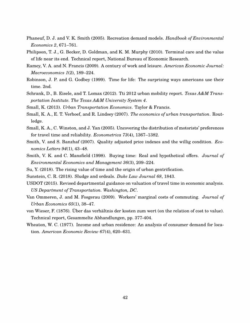
Phaneuf, D. J. and V. K. Smith (2005). Recreation demand models. Handbook of EnvironmentalEconomics 2, 671–761.
Philipson, T. J., G. Becker, D. Goldman, and K. M. Murphy (2010). Terminal care and the valueof life near its end. Technical report, National Bureau of Economic Research.
Ramey, V. A. and N. Francis (2009). A century of work and leisure. American Economic Journal:Macroeconomics 1(2), 189–224.
Robinson, J. P. and G. Godbey (1999). Time for life: The surprising ways americans use theirtime. 2nd.
Schrank, D., B. Eisele, and T. Lomax (2012). Tti 2012 urban mobility report. Texas A&M Trans-portation Institute. The Texas A&M University System 4.
Small, K. (2013). Urban Transportation Economics. Taylor & Francis.Small, K. A., E. T. Verhoef, and R. Lindsey (2007). The economics of urban transportation. Rout-ledge.
Small, K. A., C. Winston, and J. Yan (2005). Uncovering the distribution of motorists’ preferencesfor travel time and reliability. Econometrica 73(4), 1367–1382.
Smith, V. and S. Banzhaf (2007). Quality adjusted price indexes and the willig condition. Eco-nomics Letters 94(1), 43–48.
Smith, V. K. and C. Mansfield (1998). Buying time: Real and hypothetical offers. Journal ofEnvironmental Economics and Management 36(3), 209–224.
Su, Y. (2018). The rising value of time and the origin of urban gentrification.Sunstein, C. R. (2018). Sludge and ordeals. Duke Law Journal 68, 1843.USDOT (2015). Revised departmental guidance on valuation of travel time in economic analysis.US Department of Transportation. Washington, DC.
Van Ommeren, J. and M. Fosgerau (2009). Workers’ marginal costs of commuting. Journal ofUrban Economics 65(1), 38–47.
von Wieser, F. (1876). Über das verhältnis der kosten zum wert (on the relation of cost to value).Technical report, Gesammelte Abhandlungen, pp. 377-404.
Wheaton, W. C. (1977). Income and urban residence: An analysis of consumer demand for loca-tion. American Economic Review 67(4), 620–631.
42

Figures
Figure 1Screenshots of the passenger Lyft app’s user interface, at the time of the experiment. Left: nodestination entered and no Prime Time active. Middle: destination entered and no Prime Timeactive. Right: destination entered and +25% Prime Time active.
43
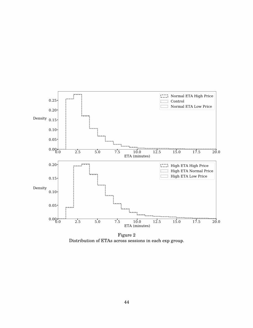
0.0 2.5 5.0 7.5 10.0 12.5 15.0 17.5 20.0ETA (minutes)
0.00
0.05
0.10
0.15
0.20
0.25
Density
Normal ETA High PriceControlNormal ETA Low Price
0.0 2.5 5.0 7.5 10.0 12.5 15.0 17.5 20.0ETA (minutes)
0.00
0.05
0.10
0.15
0.20
Density
High ETA High PriceHigh ETA Normal PriceHigh ETA Low Price
Figure 2Distribution of ETAs across sessions in each exp group.
44

0 50 100 150 200 250 300PT (%)
0.02
0.04
0.06
0.08
0.10
Density
High ETA Low PriceNormal ETA Low Price
0 50 100 150 200 250 300PT (%)
0.02
0.04
0.06
0.08
0.10
Density
High ETA Normal PriceControl
0 50 100 150 200 250 300PT (%)
0.02
0.04
0.06
0.08
0.10
Density
High ETA High PriceNormal ETA High Price
Figure 3Distribution of PT across sessions in each exp group.
45

Normal ETALow Price
Control Normal ETAHigh Price
High ETALow Price
High ETANormal Price
High ETAHigh Price
Treatment Group
0.58
0.59
0.60
0.61
0.62
0.63
0.64
AverageRequest Rate
Figure 4Average request rates across the six experimental groups. Error bars are 95% confidence inter-vals based on user-level clustered standard errors.
0 5 10 15 20 25ETA (minutes)
0.00
0.05
0.10
0.15
0.20
0.25
Density
ControlPlus 60+Plus 150+Plus 240+
Figure 5Distribution of ETAs across treatments in experiment two.
46

Control Plus 60+ Plus 150+ Plus 240+Treatment Variant
0.58
0.59
0.60
0.61
0.62
AverageRequest Rate
Figure 6Average demand across the four treatments in experiment two.
47
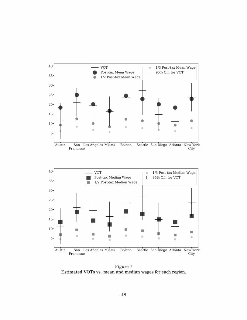
Austin SanFrancisco
Los Angeles Miami Boston Seattle San Diego Atlanta New YorkCity
5
10
15
20
25
30
35
40 VOTPost-tax Mean Wage1/2 Post-tax Mean Wage
1/3 Post-tax Mean Wage95% C.I. for VOT
Austin SanFrancisco
Los Angeles Miami Boston Seattle San Diego Atlanta New YorkCity
5
10
15
20
25
30
35
40 VOTPost-tax Median Wage1/2 Post-tax Median Wage
1/3 Post-tax Median Wage95% C.I. for VOT
Figure 7Estimated VOTs vs. mean and median wages for each region.
48
0 10 20 30 40$/hour
San Francisco
New York City
Miami
Los Angeles
Boston
Atlanta
All Six Regions
VOT (low)VOT (medium)VOT (high)Post-tax Mean Wage
95% C.I. for VOT (low)95% C.I. for VOT (medium)95% C.I. for VOT (high)
Figure 8Values of time estimated by three different treatment level contrasts.
49
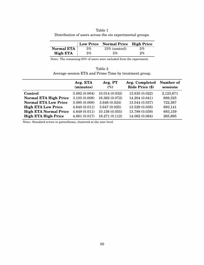
Table 1Distribution of users across the six experimental groups.
Low Price Normal Price High PriceNormal ETA 5% 15% (control) 5%High ETA 5% 5% 2%
Notes: The remaining 63% of users were excluded from the experiment.
Table 2Average session ETA and Prime Time by treatment group.
Avg. ETA(minutes)
Avg. PT(%)
Avg. CompletedRide Price ($)
Number ofsessions
Control 3.082 (0.004) 10.014 (0.032) 13.835 (0.022) 2,123,671Normal ETA High Price 3.103 (0.008) 16.362 (0.072) 14.204 (0.041) 689,325Normal ETA Low Price 3.085 (0.008) 3.646 (0.024) 13.544 (0.037) 722,367High ETA Low Price 4.640 (0.011) 3.647 (0.025) 13.529 (0.038) 693,141High ETA Normal Price 4.649 (0.011) 10.136 (0.055) 13.788 (0.039) 683,159High ETA High Price 4.661 (0.017) 16.271 (0.112) 14.062 (0.064) 265,695Notes: Standard errors in parentheses, clustered at the user level.
50
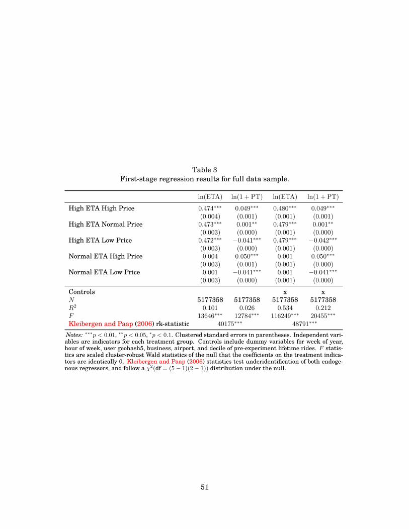
Table 3First-stage regression results for full data sample.
ln(ETA) ln(1 + PT) ln(ETA) ln(1 + PT)
High ETA High Price 0.474∗∗∗ 0.049∗∗∗ 0.480∗∗∗ 0.049∗∗∗
(0.004) (0.001) (0.001) (0.001)High ETA Normal Price 0.473∗∗∗ 0.001∗∗ 0.479∗∗∗ 0.001∗∗
(0.003) (0.000) (0.001) (0.000)High ETA Low Price 0.472∗∗∗ −0.041∗∗∗ 0.479∗∗∗ −0.042∗∗∗
(0.003) (0.000) (0.001) (0.000)Normal ETA High Price 0.004 0.050∗∗∗ 0.001 0.050∗∗∗
(0.003) (0.001) (0.001) (0.000)Normal ETA Low Price 0.001 −0.041∗∗∗ 0.001 −0.041∗∗∗
(0.003) (0.000) (0.001) (0.000)
Controls x xN 5177358 5177358 5177358 5177358R2 0.101 0.026 0.534 0.212F 13646∗∗∗ 12784∗∗∗ 116249∗∗∗ 20455∗∗∗
Kleibergen and Paap (2006) rk-statistic 40175∗∗∗ 48791∗∗∗
Notes: ∗∗∗p < 0.01, ∗∗p < 0.05, ∗p < 0.1. Clustered standard errors in parentheses. Independent vari-ables are indicators for each treatment group. Controls include dummy variables for week of year,hour of week, user geohash5, business, airport, and decile of pre-experiment lifetime rides. F statis-tics are scaled cluster-robust Wald statistics of the null that the coefficients on the treatment indica-tors are identically 0. Kleibergen and Paap (2006) statistics test underidentification of both endoge-nous regressors, and follow a χ2(df = (5− 1)(2− 1)) distribution under the null.
51
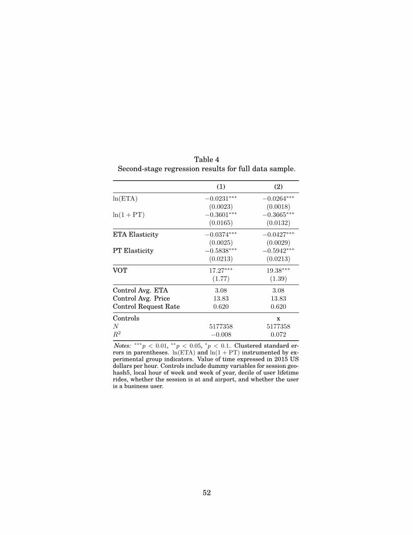
Table 4Second-stage regression results for full data sample.
(1) (2)ln(ETA) −0.0231∗∗∗ −0.0264∗∗∗
(0.0023) (0.0018)ln(1 + PT) −0.3601∗∗∗ −0.3665∗∗∗
(0.0165) (0.0132)
ETA Elasticity −0.0374∗∗∗ −0.0427∗∗∗
(0.0025) (0.0029)PT Elasticity −0.5838∗∗∗ −0.5942∗∗∗
(0.0213) (0.0213)
VOT 17.27∗∗∗ 19.38∗∗∗
(1.77) (1.39)
Control Avg. ETA 3.08 3.08Control Avg. Price 13.83 13.83Control Request Rate 0.620 0.620
Controls xN 5177358 5177358R2 −0.008 0.072Notes: ∗∗∗p < 0.01, ∗∗p < 0.05, ∗p < 0.1. Clustered standard er-rors in parentheses. ln(ETA) and ln(1 + PT) instrumented by ex-perimental group indicators. Value of time expressed in 2015 USdollars per hour. Controls include dummy variables for session geo-hash5, local hour of week and week of year, decile of user lifetimerides, whether the session is at and airport, and whether the useris a business user.
52

Table 5Summary of Elasticity and VOT Results: Features Affecting Opportunity Cost
Sub-sample ETA Elasticity PT Elasticity VOT
Full Sample −0.043∗∗∗ −0.594∗∗∗ 19.38∗∗∗(0.003) (0.021) (1.39)
Day of WeekMonday −0.048∗∗∗ −0.627∗∗∗ 20.08∗∗∗
(0.005) (0.046) (2.47)Tuesday −0.046∗∗∗ −0.676∗∗∗ 17.95∗∗∗
(0.005) (0.049) (2.22)Wednesday −0.046∗∗∗ −0.653∗∗∗ 19.34∗∗∗
(0.005) (0.048) (2.38)Thursday −0.041∗∗∗ −0.585∗∗∗ 19.44∗∗∗
(0.005) (0.035) (2.41)Friday −0.039∗∗∗ −0.473∗∗∗ 21.26∗∗∗
(0.005) (0.023) (2.45)Saturday −0.039∗∗∗ −0.596∗∗∗ 18.74∗∗∗
(0.004) (0.031) (2.04)Sunday −0.040∗∗∗ −0.640∗∗∗ 17.12∗∗∗
(0.005) (0.030) (2.01)
Time of Day (Weekends)6–10 AM −0.056∗∗∗ −0.687∗∗∗ 17.40∗∗∗
(0.011) (0.081) (3.80)10 AM–4 PM −0.053∗∗∗ −0.727∗∗∗ 18.92∗∗∗
(0.007) (0.047) (2.49)4 PM–7 PM −0.048∗∗∗ −0.616∗∗∗ 20.16∗∗∗
(0.007) (0.039) (2.92)7 PM–11 PM −0.033∗∗∗ −0.669∗∗∗ 15.04∗∗∗
(0.006) (0.062) (2.87)11 PM–6 AM −0.023∗∗∗ −0.500∗∗∗ 14.71∗∗∗
(0.005) (0.028) (3.12)
Time of Day (Weekdays)6–10 AM −0.068∗∗∗ −0.594∗∗∗ 26.71∗∗∗
(0.006) (0.034) (2.50)10 AM–4 PM −0.047∗∗∗ −0.704∗∗∗ 18.76∗∗∗
(0.006) (0.061) (2.64)4 PM–7 PM −0.046∗∗∗ −0.522∗∗∗ 22.12∗∗∗
(0.005) (0.034) (2.70)7 PM–11 PM −0.024∗∗∗ −0.540∗∗∗ 13.62∗∗∗
(0.005) (0.041) (2.59)11 PM–6 AM −0.040∗∗∗ −0.539∗∗∗ 19.03∗∗∗
(0.006) (0.031) (2.66)
Notes: ∗∗∗p < 0.01, ∗∗p < 0.05, ∗p < 0.1. Clustered standard errors inparentheses. Controls include local week of year, local hour of week,user geohash5, business user, airport, and decile of pre-experimentlifetime rides.
53

Table 6Summary of Elasticity and VOT Results: Other Trip Characteristics
Sub-sample ETA Elasticity PT Elasticity VOT
Full Sample −0.043∗∗∗ −0.594∗∗∗ 19.38∗∗∗(0.003) (0.021) (1.39)
PrecipitationNone −0.042∗∗∗ −0.597∗∗∗ 19.04∗∗∗
(0.003) (0.024) (1.50)Rain −0.051∗∗∗ −0.560∗∗∗ 23.10∗∗∗
(0.005) (0.026) (2.26)Snow −0.103∗∗∗ −0.711∗∗∗ 26.56∗∗∗
(0.029) (0.119) (7.83)
User TypeBusiness −0.033∗∗ −0.399∗∗∗ 24.42∗∗
(0.014) (0.073) (10.55)Non-Business −0.043∗∗∗ −0.605∗∗∗ 19.22∗∗∗
(0.003) (0.022) (1.39)
Notes: ∗∗∗p < 0.01, ∗∗p < 0.05, ∗p < 0.1. Clustered standarderrors in parentheses. Controls include local week of year, lo-cal hour of week, user geohash5, business user, and decile ofpre-experiment lifetime rides.
54
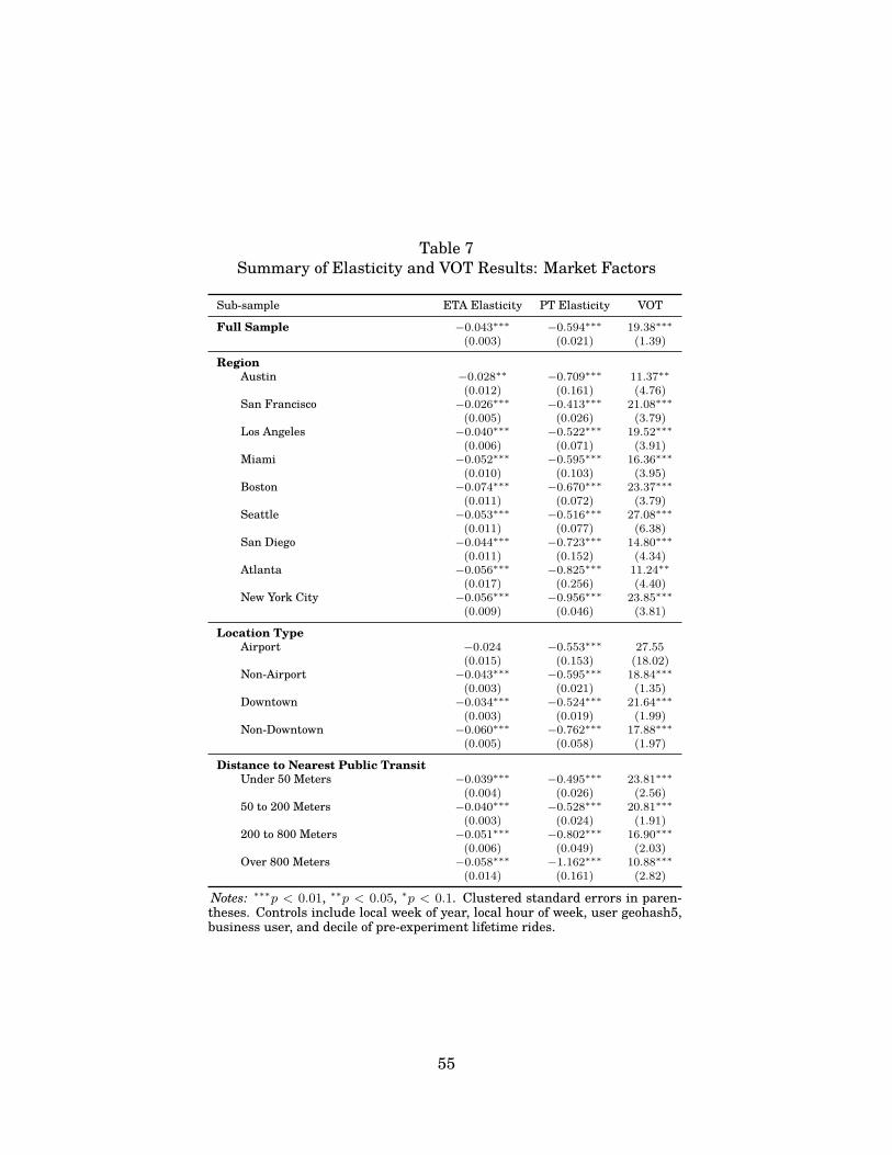
Table 7Summary of Elasticity and VOT Results: Market Factors
Sub-sample ETA Elasticity PT Elasticity VOT
Full Sample −0.043∗∗∗ −0.594∗∗∗ 19.38∗∗∗(0.003) (0.021) (1.39)
RegionAustin −0.028∗∗ −0.709∗∗∗ 11.37∗∗
(0.012) (0.161) (4.76)San Francisco −0.026∗∗∗ −0.413∗∗∗ 21.08∗∗∗
(0.005) (0.026) (3.79)Los Angeles −0.040∗∗∗ −0.522∗∗∗ 19.52∗∗∗
(0.006) (0.071) (3.91)Miami −0.052∗∗∗ −0.595∗∗∗ 16.36∗∗∗
(0.010) (0.103) (3.95)Boston −0.074∗∗∗ −0.670∗∗∗ 23.37∗∗∗
(0.011) (0.072) (3.79)Seattle −0.053∗∗∗ −0.516∗∗∗ 27.08∗∗∗
(0.011) (0.077) (6.38)San Diego −0.044∗∗∗ −0.723∗∗∗ 14.80∗∗∗
(0.011) (0.152) (4.34)Atlanta −0.056∗∗∗ −0.825∗∗∗ 11.24∗∗
(0.017) (0.256) (4.40)New York City −0.056∗∗∗ −0.956∗∗∗ 23.85∗∗∗
(0.009) (0.046) (3.81)
Location TypeAirport −0.024 −0.553∗∗∗ 27.55
(0.015) (0.153) (18.02)Non-Airport −0.043∗∗∗ −0.595∗∗∗ 18.84∗∗∗
(0.003) (0.021) (1.35)Downtown −0.034∗∗∗ −0.524∗∗∗ 21.64∗∗∗
(0.003) (0.019) (1.99)Non-Downtown −0.060∗∗∗ −0.762∗∗∗ 17.88∗∗∗
(0.005) (0.058) (1.97)
Distance to Nearest Public TransitUnder 50 Meters −0.039∗∗∗ −0.495∗∗∗ 23.81∗∗∗
(0.004) (0.026) (2.56)50 to 200 Meters −0.040∗∗∗ −0.528∗∗∗ 20.81∗∗∗
(0.003) (0.024) (1.91)200 to 800 Meters −0.051∗∗∗ −0.802∗∗∗ 16.90∗∗∗
(0.006) (0.049) (2.03)Over 800 Meters −0.058∗∗∗ −1.162∗∗∗ 10.88∗∗∗
(0.014) (0.161) (2.82)
Notes: ∗∗∗p < 0.01, ∗∗p < 0.05, ∗p < 0.1. Clustered standard errors in paren-theses. Controls include local week of year, local hour of week, user geohash5,business user, and decile of pre-experiment lifetime rides.
55

Table 8Summary of Elasticity Results: Heterogeneity (2017 Experiment)
Time of Week (1) Trip Characteristics (2) Location (3)
Full Sample −0.043∗∗∗ Full Sample −0.043∗∗∗ Full Sample −0.043∗∗∗(0.001) (0.001) (0.001)
Day of Week Precipitation RegionMonday −0.044∗∗∗ None −0.042∗∗∗ San Francisco −0.031∗∗∗
(0.002) (0.001) (0.001)Tuesday −0.047∗∗∗ Rain −0.047∗∗∗ New York City −0.086∗∗∗
(0.002) (0.002) (0.002)Wednesday −0.044∗∗∗ Chicago −0.039∗∗∗
(0.002) User Type (0.002)Thursday −0.047∗∗∗ Business −0.049∗∗∗ Washington, D.C. −0.054∗∗∗
(0.002) (0.002) (0.002)Friday −0.042∗∗∗ Non-Business −0.043∗∗∗ Miami −0.021∗∗∗
(0.002) (0.001) (0.002)Saturday −0.039∗∗∗ New Jersey −0.053∗∗∗
(0.002) (0.004)Sunday −0.040∗∗∗ Boston −0.055∗∗∗
(0.002) (0.003)Philadelphia −0.040∗∗∗
Time of Day (Weekends) (0.003)6–10 AM −0.060∗∗∗ Atlanta −0.037∗∗∗
(0.004) (0.004)10 AM–4 PM −0.048∗∗∗ Los Angeles −0.033∗∗∗
(0.003) (0.002)4 PM–7 PM −0.044∗∗∗
(0.003) Location Type7 PM–11 PM −0.033∗∗∗ Downtown −0.039∗∗∗
(0.003) (0.001)11 PM–6 AM −0.026∗∗∗ Non-Downtown −0.048∗∗∗
(0.002) (0.001)
Time of Day (Weekdays) Distance to Public Transit6–10 AM −0.061∗∗∗ Under 50 Meters −0.042∗∗∗
(0.002) (0.001)10 AM–4 PM −0.041∗∗∗ 50 to 200 Meters −0.038∗∗∗
(0.002) (0.001)4 PM–7 PM −0.052∗∗∗ 200 to 800 Meters −0.049∗∗∗
(0.002) (0.002)7 PM–11 PM −0.035∗∗∗ Over 800 Meters −0.084∗∗∗
(0.002) (0.004)11 PM–6 AM −0.037∗∗∗
(0.002)
Notes: ∗∗∗p < 0.01, ∗∗p < 0.05, ∗p < 0.1. Clustered standard errors in parentheses. Controls include local week ofyear, local hour of week, user geohash5, business user, and decile of pre-experiment lifetime rides.
56
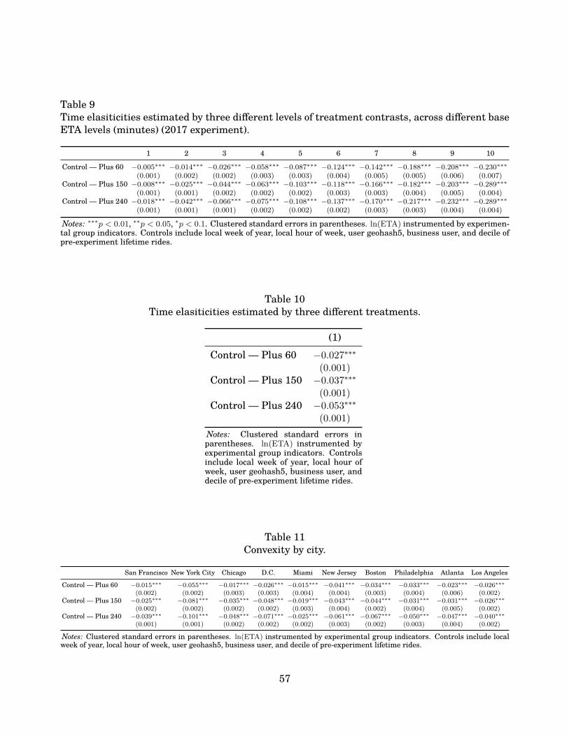
Table 9Time elasiticities estimated by three different levels of treatment contrasts, across different baseETA levels (minutes) (2017 experiment).
1 2 3 4 5 6 7 8 9 10
Control — Plus 60 −0.005∗∗∗ −0.014∗∗∗ −0.026∗∗∗ −0.058∗∗∗ −0.087∗∗∗ −0.124∗∗∗ −0.142∗∗∗ −0.188∗∗∗ −0.208∗∗∗ −0.230∗∗∗(0.001) (0.002) (0.002) (0.003) (0.003) (0.004) (0.005) (0.005) (0.006) (0.007)
Control — Plus 150 −0.008∗∗∗ −0.025∗∗∗ −0.044∗∗∗ −0.063∗∗∗ −0.103∗∗∗ −0.118∗∗∗ −0.166∗∗∗ −0.182∗∗∗ −0.203∗∗∗ −0.289∗∗∗(0.001) (0.001) (0.002) (0.002) (0.002) (0.003) (0.003) (0.004) (0.005) (0.004)
Control — Plus 240 −0.018∗∗∗ −0.042∗∗∗ −0.066∗∗∗ −0.075∗∗∗ −0.108∗∗∗ −0.137∗∗∗ −0.170∗∗∗ −0.217∗∗∗ −0.232∗∗∗ −0.289∗∗∗(0.001) (0.001) (0.001) (0.002) (0.002) (0.002) (0.003) (0.003) (0.004) (0.004)
Notes: ∗∗∗p < 0.01, ∗∗p < 0.05, ∗p < 0.1. Clustered standard errors in parentheses. ln(ETA) instrumented by experimen-tal group indicators. Controls include local week of year, local hour of week, user geohash5, business user, and decile ofpre-experiment lifetime rides.
Table 10Time elasiticities estimated by three different treatments.
(1)Control — Plus 60 −0.027∗∗∗
(0.001)Control — Plus 150 −0.037∗∗∗
(0.001)Control — Plus 240 −0.053∗∗∗
(0.001)Notes: Clustered standard errors inparentheses. ln(ETA) instrumented byexperimental group indicators. Controlsinclude local week of year, local hour ofweek, user geohash5, business user, anddecile of pre-experiment lifetime rides.
Table 11Convexity by city.
San Francisco New York City Chicago D.C. Miami New Jersey Boston Philadelphia Atlanta Los Angeles
Control — Plus 60 −0.015∗∗∗ −0.055∗∗∗ −0.017∗∗∗ −0.026∗∗∗ −0.015∗∗∗ −0.041∗∗∗ −0.034∗∗∗ −0.033∗∗∗ −0.023∗∗∗ −0.026∗∗∗(0.002) (0.002) (0.003) (0.003) (0.004) (0.004) (0.003) (0.004) (0.006) (0.002)
Control — Plus 150 −0.025∗∗∗ −0.081∗∗∗ −0.035∗∗∗ −0.048∗∗∗ −0.019∗∗∗ −0.043∗∗∗ −0.044∗∗∗ −0.031∗∗∗ −0.031∗∗∗ −0.026∗∗∗(0.002) (0.002) (0.002) (0.002) (0.003) (0.004) (0.002) (0.004) (0.005) (0.002)
Control — Plus 240 −0.039∗∗∗ −0.101∗∗∗ −0.048∗∗∗ −0.071∗∗∗ −0.025∗∗∗ −0.061∗∗∗ −0.067∗∗∗ −0.050∗∗∗ −0.047∗∗∗ −0.040∗∗∗(0.001) (0.001) (0.002) (0.002) (0.002) (0.003) (0.002) (0.003) (0.004) (0.002)
Notes: Clustered standard errors in parentheses. ln(ETA) instrumented by experimental group indicators. Controls include localweek of year, local hour of week, user geohash5, business user, and decile of pre-experiment lifetime rides.
57
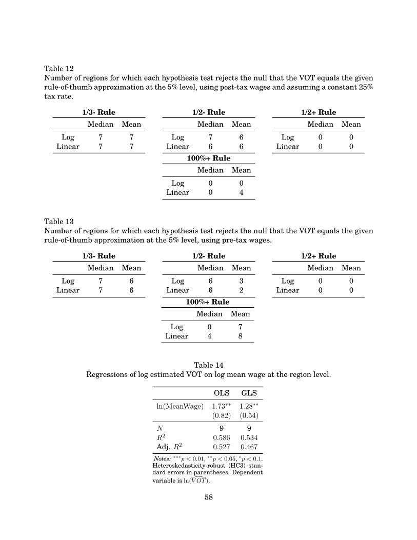
Table 12Number of regions for which each hypothesis test rejects the null that the VOT equals the givenrule-of-thumb approximation at the 5% level, using post-tax wages and assuming a constant 25%tax rate.
1/3- RuleMedian Mean
Log 7 7Linear 7 7
1/2- RuleMedian Mean
Log 7 6Linear 6 6
1/2+ RuleMedian Mean
Log 0 0Linear 0 0
100%+ RuleMedian Mean
Log 0 0Linear 0 4
Table 13Number of regions for which each hypothesis test rejects the null that the VOT equals the givenrule-of-thumb approximation at the 5% level, using pre-tax wages.
1/3- RuleMedian Mean
Log 7 6Linear 7 6
1/2- RuleMedian Mean
Log 6 3Linear 6 2
1/2+ RuleMedian Mean
Log 0 0Linear 0 0
100%+ RuleMedian Mean
Log 0 7Linear 4 8
Table 14Regressions of log estimated VOT on log mean wage at the region level.
OLS GLSln(MeanWage) 1.73∗∗ 1.28∗∗
(0.82) (0.54)
N 9 9R2 0.586 0.534Adj. R2 0.527 0.467Notes: ∗∗∗p < 0.01, ∗∗p < 0.05, ∗p < 0.1.Heteroskedasticity-robust (HC3) stan-dard errors in parentheses. Dependentvariable is ln(V̂ OT ).
58