Working Backwards with the Normal Distribution

Average IQ Scores by Country 2021 Average IQ by State 2021

IQ Classifications

IQ Scores are Normally Distributed with a mean of 100 and a standard deviation of 15.

What IQ Score is needed to be considered a Genius?

What IQ Score is needed to be eligible for MENSA membership?

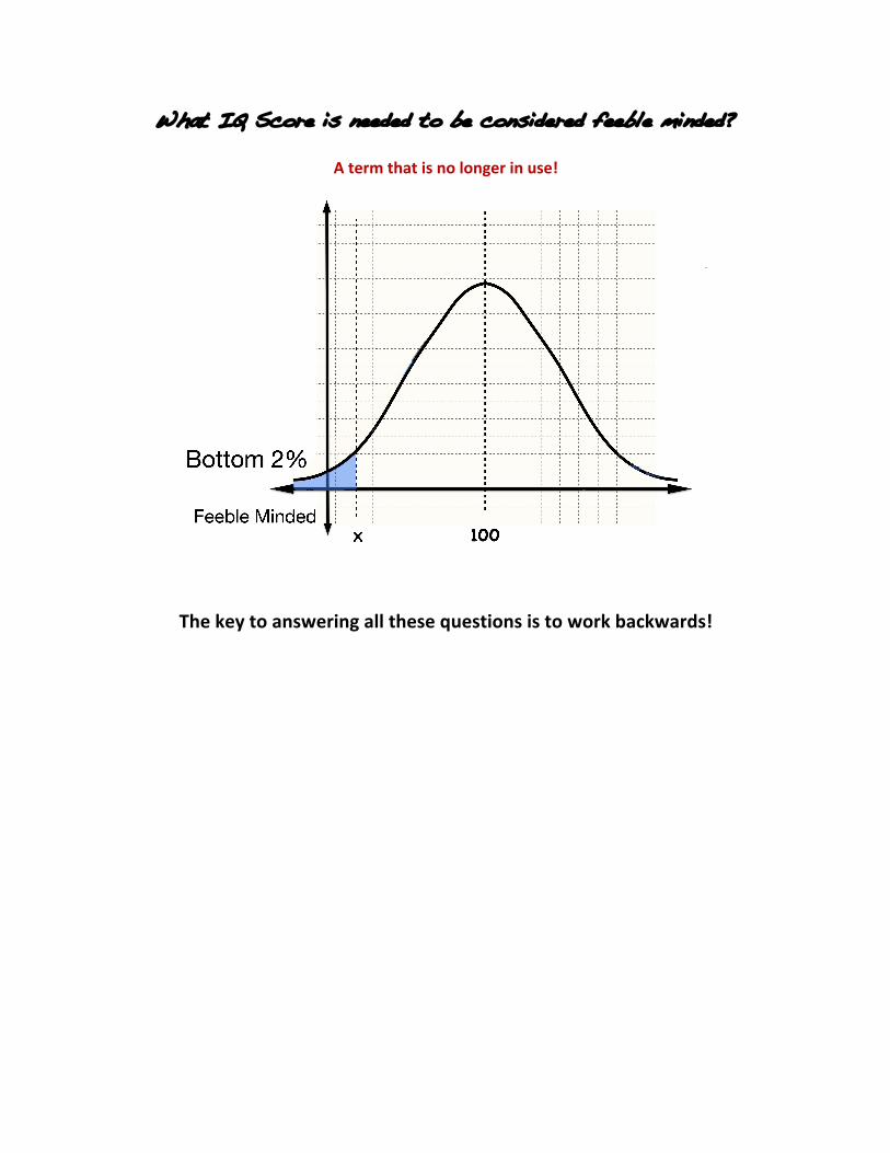
What IQ Score is needed to be considered feeble minded?

A term that is no longer in use!

The key to answering all these questions is to work backwards!

0 z

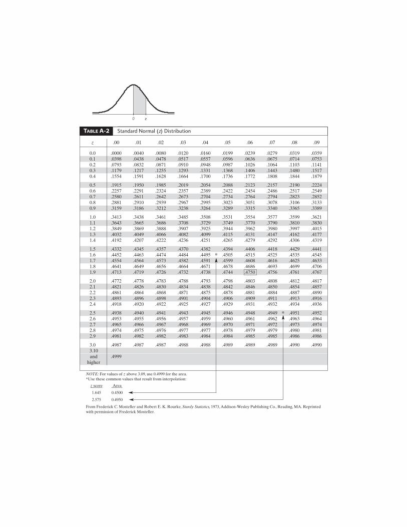
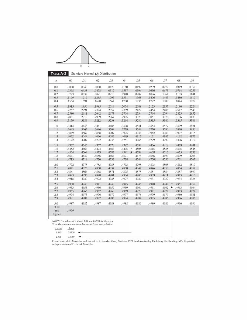
TABLE A-2 Standard Normal (z) Distribution

z .00 .01 .02 .03 .04 .05 .06 .07 .08 .09

0.0 .0000 .0040 .0080 .0120 .0160 .0199 .0239 .0279 .0319 .03590.1 .0398 .0438 .0478 .0517 .0557 .0596 .0636 .0675 .0714 .07530.2 .0793 .0832 .0871 .0910 .0948 .0987 .1026 .1064 .1103 .11410.3 .1179 .1217 .1255 .1293 .1331 .1368 .1406 .1443 .1480 .15170.4 .1554 .1591 .1628 .1664 .1700 .1736 .1772 .1808 .1844 .1879

0.5 .1915 .1950 .1985 .2019 .2054 .2088 .2123 .2157 .2190 .22240.6 .2257 .2291 .2324 .2357 .2389 .2422 .2454 .2486 .2517 .25490.7 .2580 .2611 .2642 .2673 .2704 .2734 .2764 .2794 .2823 .28520.8 .2881 .2910 .2939 .2967 .2995 .3023 .3051 .3078 .3106 .31330.9 .3159 .3186 .3212 .3238 .3264 .3289 .3315 .3340 .3365 .3389

1.0 .3413 .3438 .3461 .3485 .3508 .3531 .3554 .3577 .3599 .36211.1 .3643 .3665 .3686 .3708 .3729 .3749 .3770 .3790 .3810 .38301.2 .3849 .3869 .3888 .3907 .3925 .3944 .3962 .3980 .3997 .40151.3 .4032 .4049 .4066 .4082 .4099 .4115 .4131 .4147 .4162 .41771.4 .4192 .4207 .4222 .4236 .4251 .4265 .4279 .4292 .4306 .4319

1.5 .4332 .4345 .4357 .4370 .4382 .4394 .4406 .4418 .4429 .44411.6 .4452 .4463 .4474 .4484 .4495 ∗ .4505 .4515 .4525 .4535 .45451.7 .4554 .4564 .4573 .4582 .4591 .4599 .4608 .4616 .4625 .46331.8 .4641 .4649 .4656 .4664 .4671 .4678 .4686 .4693 .4699 .47061.9 .4713 .4719 .4726 .4732 .4738 .4744 .4750 .4756 .4761 .4767

2.0 .4772 .4778 .4783 .4788 .4793 .4798 .4803 .4808 .4812 .48172.1 .4821 .4826 .4830 .4834 .4838 .4842 .4846 .4850 .4854 .48572.2 .4861 .4864 .4868 .4871 .4875 .4878 .4881 .4884 .4887 .48902.3 .4893 .4896 .4898 .4901 .4904 .4906 .4909 .4911 .4913 .49162.4 .4918 .4920 .4922 .4925 .4927 .4929 .4931 .4932 .4934 .4936

2.5 .4938 .4940 .4941 .4943 .4945 .4946 .4948 .4949 ∗ .4951 .49522.6 .4953 .4955 .4956 .4957 .4959 .4960 .4961 .4962 .4963 .49642.7 .4965 .4966 .4967 .4968 .4969 .4970 .4971 .4972 .4973 .49742.8 .4974 .4975 .4976 .4977 .4977 .4978 .4979 .4979 .4980 .49812.9 .4981 .4982 .4982 .4983 .4984 .4984 .4985 .4985 .4986 .4986

3.0 .4987 .4987 .4987 .4988 .4988 .4989 .4989 .4989 .4990 .49903.10 and .4999

higher

NOTE: For values of z above 3.09, use 0.4999 for the area.*Use these common values that result from interpolation:

z score Area

1.645 0.4500

2.575 0.4950

From Frederick C. Mosteller and Robert E. K. Rourke, Sturdy Statistics, 1973, Addison-Wesley Publishing Co., Reading, MA. Reprintedwith permission of Frederick Mosteller.

What z value is associated with finding the following shaded portions of the bell? To answer these questions we will need to work backwards with our z table. Top 1%

Use the z table working backwards to determine the z value that represents 49% of the bell being shaded.

0 z

TABLE A-2 Standard Normal (z) Distribution

z .00 .01 .02 .03 .04 .05 .06 .07 .08 .09

0.0 .0000 .0040 .0080 .0120 .0160 .0199 .0239 .0279 .0319 .03590.1 .0398 .0438 .0478 .0517 .0557 .0596 .0636 .0675 .0714 .07530.2 .0793 .0832 .0871 .0910 .0948 .0987 .1026 .1064 .1103 .11410.3 .1179 .1217 .1255 .1293 .1331 .1368 .1406 .1443 .1480 .15170.4 .1554 .1591 .1628 .1664 .1700 .1736 .1772 .1808 .1844 .1879

0.5 .1915 .1950 .1985 .2019 .2054 .2088 .2123 .2157 .2190 .22240.6 .2257 .2291 .2324 .2357 .2389 .2422 .2454 .2486 .2517 .25490.7 .2580 .2611 .2642 .2673 .2704 .2734 .2764 .2794 .2823 .28520.8 .2881 .2910 .2939 .2967 .2995 .3023 .3051 .3078 .3106 .31330.9 .3159 .3186 .3212 .3238 .3264 .3289 .3315 .3340 .3365 .3389

1.0 .3413 .3438 .3461 .3485 .3508 .3531 .3554 .3577 .3599 .36211.1 .3643 .3665 .3686 .3708 .3729 .3749 .3770 .3790 .3810 .38301.2 .3849 .3869 .3888 .3907 .3925 .3944 .3962 .3980 .3997 .40151.3 .4032 .4049 .4066 .4082 .4099 .4115 .4131 .4147 .4162 .41771.4 .4192 .4207 .4222 .4236 .4251 .4265 .4279 .4292 .4306 .4319

1.5 .4332 .4345 .4357 .4370 .4382 .4394 .4406 .4418 .4429 .44411.6 .4452 .4463 .4474 .4484 .4495 ∗ .4505 .4515 .4525 .4535 .45451.7 .4554 .4564 .4573 .4582 .4591 .4599 .4608 .4616 .4625 .46331.8 .4641 .4649 .4656 .4664 .4671 .4678 .4686 .4693 .4699 .47061.9 .4713 .4719 .4726 .4732 .4738 .4744 .4750 .4756 .4761 .4767

2.0 .4772 .4778 .4783 .4788 .4793 .4798 .4803 .4808 .4812 .48172.1 .4821 .4826 .4830 .4834 .4838 .4842 .4846 .4850 .4854 .48572.2 .4861 .4864 .4868 .4871 .4875 .4878 .4881 .4884 .4887 .48902.3 .4893 .4896 .4898 .4901 .4904 .4906 .4909 .4911 .4913 .49162.4 .4918 .4920 .4922 .4925 .4927 .4929 .4931 .4932 .4934 .4936

2.5 .4938 .4940 .4941 .4943 .4945 .4946 .4948 .4949 ∗ .4951 .49522.6 .4953 .4955 .4956 .4957 .4959 .4960 .4961 .4962 .4963 .49642.7 .4965 .4966 .4967 .4968 .4969 .4970 .4971 .4972 .4973 .49742.8 .4974 .4975 .4976 .4977 .4977 .4978 .4979 .4979 .4980 .49812.9 .4981 .4982 .4982 .4983 .4984 .4984 .4985 .4985 .4986 .4986

3.0 .4987 .4987 .4987 .4988 .4988 .4989 .4989 .4989 .4990 .49903.10 and .4999

higher

NOTE: For values of z above 3.09, use 0.4999 for the area.*Use these common values that result from interpolation:

z score Area

1.645 0.4500

2.575 0.4950

From Frederick C. Mosteller and Robert E. K. Rourke, Sturdy Statistics, 1973, Addison-Wesley Publishing Co., Reading, MA. Reprintedwith permission of Frederick Mosteller.

Top 1%

TI-83 or TI-84 Plus Finding the z vaue corresponding to a known area. 1. Press 2nd then vars to access DISTR (distributions) menu. 2. Select InvNorm and click enter. 3. Enter the area to the left of the z value, enter the mean 𝜇, enter the standard deviation 𝜎

InvNorm(area to the left,𝝁,𝝈) and press enter

InvNorm (0.99,0,1)

Bottom 1% or the 1st Percentile

Use the z table working backwards to determine the z value that represents 49% of the bell being shaded.

0 z

TABLE A-2 Standard Normal (z) Distribution

z .00 .01 .02 .03 .04 .05 .06 .07 .08 .09

0.0 .0000 .0040 .0080 .0120 .0160 .0199 .0239 .0279 .0319 .03590.1 .0398 .0438 .0478 .0517 .0557 .0596 .0636 .0675 .0714 .07530.2 .0793 .0832 .0871 .0910 .0948 .0987 .1026 .1064 .1103 .11410.3 .1179 .1217 .1255 .1293 .1331 .1368 .1406 .1443 .1480 .15170.4 .1554 .1591 .1628 .1664 .1700 .1736 .1772 .1808 .1844 .1879

0.5 .1915 .1950 .1985 .2019 .2054 .2088 .2123 .2157 .2190 .22240.6 .2257 .2291 .2324 .2357 .2389 .2422 .2454 .2486 .2517 .25490.7 .2580 .2611 .2642 .2673 .2704 .2734 .2764 .2794 .2823 .28520.8 .2881 .2910 .2939 .2967 .2995 .3023 .3051 .3078 .3106 .31330.9 .3159 .3186 .3212 .3238 .3264 .3289 .3315 .3340 .3365 .3389

1.0 .3413 .3438 .3461 .3485 .3508 .3531 .3554 .3577 .3599 .36211.1 .3643 .3665 .3686 .3708 .3729 .3749 .3770 .3790 .3810 .38301.2 .3849 .3869 .3888 .3907 .3925 .3944 .3962 .3980 .3997 .40151.3 .4032 .4049 .4066 .4082 .4099 .4115 .4131 .4147 .4162 .41771.4 .4192 .4207 .4222 .4236 .4251 .4265 .4279 .4292 .4306 .4319

1.5 .4332 .4345 .4357 .4370 .4382 .4394 .4406 .4418 .4429 .44411.6 .4452 .4463 .4474 .4484 .4495 ∗ .4505 .4515 .4525 .4535 .45451.7 .4554 .4564 .4573 .4582 .4591 .4599 .4608 .4616 .4625 .46331.8 .4641 .4649 .4656 .4664 .4671 .4678 .4686 .4693 .4699 .47061.9 .4713 .4719 .4726 .4732 .4738 .4744 .4750 .4756 .4761 .4767

2.0 .4772 .4778 .4783 .4788 .4793 .4798 .4803 .4808 .4812 .48172.1 .4821 .4826 .4830 .4834 .4838 .4842 .4846 .4850 .4854 .48572.2 .4861 .4864 .4868 .4871 .4875 .4878 .4881 .4884 .4887 .48902.3 .4893 .4896 .4898 .4901 .4904 .4906 .4909 .4911 .4913 .49162.4 .4918 .4920 .4922 .4925 .4927 .4929 .4931 .4932 .4934 .4936

2.5 .4938 .4940 .4941 .4943 .4945 .4946 .4948 .4949 ∗ .4951 .49522.6 .4953 .4955 .4956 .4957 .4959 .4960 .4961 .4962 .4963 .49642.7 .4965 .4966 .4967 .4968 .4969 .4970 .4971 .4972 .4973 .49742.8 .4974 .4975 .4976 .4977 .4977 .4978 .4979 .4979 .4980 .49812.9 .4981 .4982 .4982 .4983 .4984 .4984 .4985 .4985 .4986 .4986

3.0 .4987 .4987 .4987 .4988 .4988 .4989 .4989 .4989 .4990 .49903.10 and .4999

higher

NOTE: For values of z above 3.09, use 0.4999 for the area.*Use these common values that result from interpolation:

z score Area

1.645 0.4500

2.575 0.4950

From Frederick C. Mosteller and Robert E. K. Rourke, Sturdy Statistics, 1973, Addison-Wesley Publishing Co., Reading, MA. Reprintedwith permission of Frederick Mosteller.

Bottom 1% or the 1st Percentile

TI-83 or TI-84 Plus Finding the z vaue corresponding to a known area. 1. Press 2nd then vars to access DISTR (distributions) menu. 2. Select InvNorm and click enter. 3. Enter the area to the left of the z value, enter the mean 𝜇, enter the standard deviation 𝜎

InvNorm(area to the left,𝝁,𝝈) and press enter

InvNorm (0.01,0,1)

Top 5%

Use the z table working backwards to determine the z value that represents 45% of the bell being shaded.

0 z

TABLE A-2 Standard Normal (z) Distribution

z .00 .01 .02 .03 .04 .05 .06 .07 .08 .09

0.0 .0000 .0040 .0080 .0120 .0160 .0199 .0239 .0279 .0319 .03590.1 .0398 .0438 .0478 .0517 .0557 .0596 .0636 .0675 .0714 .07530.2 .0793 .0832 .0871 .0910 .0948 .0987 .1026 .1064 .1103 .11410.3 .1179 .1217 .1255 .1293 .1331 .1368 .1406 .1443 .1480 .15170.4 .1554 .1591 .1628 .1664 .1700 .1736 .1772 .1808 .1844 .1879

0.5 .1915 .1950 .1985 .2019 .2054 .2088 .2123 .2157 .2190 .22240.6 .2257 .2291 .2324 .2357 .2389 .2422 .2454 .2486 .2517 .25490.7 .2580 .2611 .2642 .2673 .2704 .2734 .2764 .2794 .2823 .28520.8 .2881 .2910 .2939 .2967 .2995 .3023 .3051 .3078 .3106 .31330.9 .3159 .3186 .3212 .3238 .3264 .3289 .3315 .3340 .3365 .3389

1.0 .3413 .3438 .3461 .3485 .3508 .3531 .3554 .3577 .3599 .36211.1 .3643 .3665 .3686 .3708 .3729 .3749 .3770 .3790 .3810 .38301.2 .3849 .3869 .3888 .3907 .3925 .3944 .3962 .3980 .3997 .40151.3 .4032 .4049 .4066 .4082 .4099 .4115 .4131 .4147 .4162 .41771.4 .4192 .4207 .4222 .4236 .4251 .4265 .4279 .4292 .4306 .4319

1.5 .4332 .4345 .4357 .4370 .4382 .4394 .4406 .4418 .4429 .44411.6 .4452 .4463 .4474 .4484 .4495 ∗ .4505 .4515 .4525 .4535 .45451.7 .4554 .4564 .4573 .4582 .4591 .4599 .4608 .4616 .4625 .46331.8 .4641 .4649 .4656 .4664 .4671 .4678 .4686 .4693 .4699 .47061.9 .4713 .4719 .4726 .4732 .4738 .4744 .4750 .4756 .4761 .4767

2.0 .4772 .4778 .4783 .4788 .4793 .4798 .4803 .4808 .4812 .48172.1 .4821 .4826 .4830 .4834 .4838 .4842 .4846 .4850 .4854 .48572.2 .4861 .4864 .4868 .4871 .4875 .4878 .4881 .4884 .4887 .48902.3 .4893 .4896 .4898 .4901 .4904 .4906 .4909 .4911 .4913 .49162.4 .4918 .4920 .4922 .4925 .4927 .4929 .4931 .4932 .4934 .4936

2.5 .4938 .4940 .4941 .4943 .4945 .4946 .4948 .4949 ∗ .4951 .49522.6 .4953 .4955 .4956 .4957 .4959 .4960 .4961 .4962 .4963 .49642.7 .4965 .4966 .4967 .4968 .4969 .4970 .4971 .4972 .4973 .49742.8 .4974 .4975 .4976 .4977 .4977 .4978 .4979 .4979 .4980 .49812.9 .4981 .4982 .4982 .4983 .4984 .4984 .4985 .4985 .4986 .4986

3.0 .4987 .4987 .4987 .4988 .4988 .4989 .4989 .4989 .4990 .49903.10 and .4999

higher

NOTE: For values of z above 3.09, use 0.4999 for the area.*Use these common values that result from interpolation:

z score Area

1.645 0.4500

2.575 0.4950

From Frederick C. Mosteller and Robert E. K. Rourke, Sturdy Statistics, 1973, Addison-Wesley Publishing Co., Reading, MA. Reprintedwith permission of Frederick Mosteller.

Top 5%

TI-83 or TI-84 Plus Finding the z vaue corresponding to a known area. 1. Press 2nd then vars to access DISTR (distributions) menu. 2. Select InvNorm and click enter. 3. Enter the area to the left of the z value, enter the mean 𝜇, enter the standard deviation 𝜎

InvNorm(area to the left,𝝁,𝝈) and press enter

InvNorm (0.95,0,1)

Bottom 5% or the 5th Percentile

Use the z table working backwards to determine the z value that represents 45% of the bell being shaded along with symmetry to determine a negative z value.

0 z

TABLE A-2 Standard Normal (z) Distribution

z .00 .01 .02 .03 .04 .05 .06 .07 .08 .09

0.0 .0000 .0040 .0080 .0120 .0160 .0199 .0239 .0279 .0319 .03590.1 .0398 .0438 .0478 .0517 .0557 .0596 .0636 .0675 .0714 .07530.2 .0793 .0832 .0871 .0910 .0948 .0987 .1026 .1064 .1103 .11410.3 .1179 .1217 .1255 .1293 .1331 .1368 .1406 .1443 .1480 .15170.4 .1554 .1591 .1628 .1664 .1700 .1736 .1772 .1808 .1844 .1879

0.5 .1915 .1950 .1985 .2019 .2054 .2088 .2123 .2157 .2190 .22240.6 .2257 .2291 .2324 .2357 .2389 .2422 .2454 .2486 .2517 .25490.7 .2580 .2611 .2642 .2673 .2704 .2734 .2764 .2794 .2823 .28520.8 .2881 .2910 .2939 .2967 .2995 .3023 .3051 .3078 .3106 .31330.9 .3159 .3186 .3212 .3238 .3264 .3289 .3315 .3340 .3365 .3389

1.0 .3413 .3438 .3461 .3485 .3508 .3531 .3554 .3577 .3599 .36211.1 .3643 .3665 .3686 .3708 .3729 .3749 .3770 .3790 .3810 .38301.2 .3849 .3869 .3888 .3907 .3925 .3944 .3962 .3980 .3997 .40151.3 .4032 .4049 .4066 .4082 .4099 .4115 .4131 .4147 .4162 .41771.4 .4192 .4207 .4222 .4236 .4251 .4265 .4279 .4292 .4306 .4319

1.5 .4332 .4345 .4357 .4370 .4382 .4394 .4406 .4418 .4429 .44411.6 .4452 .4463 .4474 .4484 .4495 ∗ .4505 .4515 .4525 .4535 .45451.7 .4554 .4564 .4573 .4582 .4591 .4599 .4608 .4616 .4625 .46331.8 .4641 .4649 .4656 .4664 .4671 .4678 .4686 .4693 .4699 .47061.9 .4713 .4719 .4726 .4732 .4738 .4744 .4750 .4756 .4761 .4767

2.0 .4772 .4778 .4783 .4788 .4793 .4798 .4803 .4808 .4812 .48172.1 .4821 .4826 .4830 .4834 .4838 .4842 .4846 .4850 .4854 .48572.2 .4861 .4864 .4868 .4871 .4875 .4878 .4881 .4884 .4887 .48902.3 .4893 .4896 .4898 .4901 .4904 .4906 .4909 .4911 .4913 .49162.4 .4918 .4920 .4922 .4925 .4927 .4929 .4931 .4932 .4934 .4936

2.5 .4938 .4940 .4941 .4943 .4945 .4946 .4948 .4949 ∗ .4951 .49522.6 .4953 .4955 .4956 .4957 .4959 .4960 .4961 .4962 .4963 .49642.7 .4965 .4966 .4967 .4968 .4969 .4970 .4971 .4972 .4973 .49742.8 .4974 .4975 .4976 .4977 .4977 .4978 .4979 .4979 .4980 .49812.9 .4981 .4982 .4982 .4983 .4984 .4984 .4985 .4985 .4986 .4986

3.0 .4987 .4987 .4987 .4988 .4988 .4989 .4989 .4989 .4990 .49903.10 and .4999

higher

NOTE: For values of z above 3.09, use 0.4999 for the area.*Use these common values that result from interpolation:

z score Area

1.645 0.4500

2.575 0.4950

From Frederick C. Mosteller and Robert E. K. Rourke, Sturdy Statistics, 1973, Addison-Wesley Publishing Co., Reading, MA. Reprintedwith permission of Frederick Mosteller.

Bottom 5% or the 5th Percentile

TI-83 or TI-84 Plus Finding the z vaue corresponding to a known area. 1. Press 2nd then vars to access DISTR (distributions) menu. 2. Select InvNorm and click enter. 3. Enter the area to the left of the z value, enter the mean 𝜇, enter the standard deviation 𝜎

InvNorm(area to the left,𝝁,𝝈) and press enter

InvNorm (0.05,0,1)

Top 10%

Use the z table working backwards to determine the z value that represents 40% of the bell being shaded.

0 z

TABLE A-2 Standard Normal (z) Distribution

z .00 .01 .02 .03 .04 .05 .06 .07 .08 .09

0.0 .0000 .0040 .0080 .0120 .0160 .0199 .0239 .0279 .0319 .03590.1 .0398 .0438 .0478 .0517 .0557 .0596 .0636 .0675 .0714 .07530.2 .0793 .0832 .0871 .0910 .0948 .0987 .1026 .1064 .1103 .11410.3 .1179 .1217 .1255 .1293 .1331 .1368 .1406 .1443 .1480 .15170.4 .1554 .1591 .1628 .1664 .1700 .1736 .1772 .1808 .1844 .1879

0.5 .1915 .1950 .1985 .2019 .2054 .2088 .2123 .2157 .2190 .22240.6 .2257 .2291 .2324 .2357 .2389 .2422 .2454 .2486 .2517 .25490.7 .2580 .2611 .2642 .2673 .2704 .2734 .2764 .2794 .2823 .28520.8 .2881 .2910 .2939 .2967 .2995 .3023 .3051 .3078 .3106 .31330.9 .3159 .3186 .3212 .3238 .3264 .3289 .3315 .3340 .3365 .3389

1.0 .3413 .3438 .3461 .3485 .3508 .3531 .3554 .3577 .3599 .36211.1 .3643 .3665 .3686 .3708 .3729 .3749 .3770 .3790 .3810 .38301.2 .3849 .3869 .3888 .3907 .3925 .3944 .3962 .3980 .3997 .40151.3 .4032 .4049 .4066 .4082 .4099 .4115 .4131 .4147 .4162 .41771.4 .4192 .4207 .4222 .4236 .4251 .4265 .4279 .4292 .4306 .4319

1.5 .4332 .4345 .4357 .4370 .4382 .4394 .4406 .4418 .4429 .44411.6 .4452 .4463 .4474 .4484 .4495 ∗ .4505 .4515 .4525 .4535 .45451.7 .4554 .4564 .4573 .4582 .4591 .4599 .4608 .4616 .4625 .46331.8 .4641 .4649 .4656 .4664 .4671 .4678 .4686 .4693 .4699 .47061.9 .4713 .4719 .4726 .4732 .4738 .4744 .4750 .4756 .4761 .4767

2.0 .4772 .4778 .4783 .4788 .4793 .4798 .4803 .4808 .4812 .48172.1 .4821 .4826 .4830 .4834 .4838 .4842 .4846 .4850 .4854 .48572.2 .4861 .4864 .4868 .4871 .4875 .4878 .4881 .4884 .4887 .48902.3 .4893 .4896 .4898 .4901 .4904 .4906 .4909 .4911 .4913 .49162.4 .4918 .4920 .4922 .4925 .4927 .4929 .4931 .4932 .4934 .4936

2.5 .4938 .4940 .4941 .4943 .4945 .4946 .4948 .4949 ∗ .4951 .49522.6 .4953 .4955 .4956 .4957 .4959 .4960 .4961 .4962 .4963 .49642.7 .4965 .4966 .4967 .4968 .4969 .4970 .4971 .4972 .4973 .49742.8 .4974 .4975 .4976 .4977 .4977 .4978 .4979 .4979 .4980 .49812.9 .4981 .4982 .4982 .4983 .4984 .4984 .4985 .4985 .4986 .4986

3.0 .4987 .4987 .4987 .4988 .4988 .4989 .4989 .4989 .4990 .49903.10 and .4999

higher

NOTE: For values of z above 3.09, use 0.4999 for the area.*Use these common values that result from interpolation:

z score Area

1.645 0.4500

2.575 0.4950

From Frederick C. Mosteller and Robert E. K. Rourke, Sturdy Statistics, 1973, Addison-Wesley Publishing Co., Reading, MA. Reprintedwith permission of Frederick Mosteller.

Top 10%

TI-83 or TI-84 Plus Finding the z vaue corresponding to a known area. 1. Press 2nd then vars to access DISTR (distributions) menu. 2. Select InvNorm and click enter. 3. Enter the area to the left of the z value, enter the mean 𝜇, enter the standard deviation 𝜎

InvNorm(area to the left,𝝁,𝝈) and press enter

InvNorm (0.90,0,1)

Bottom 10% or 1st Decile

Use the z table working backwards to determine the z value that represents 40% of the bell being shaded.

0 z

TABLE A-2 Standard Normal (z) Distribution

z .00 .01 .02 .03 .04 .05 .06 .07 .08 .09

0.0 .0000 .0040 .0080 .0120 .0160 .0199 .0239 .0279 .0319 .03590.1 .0398 .0438 .0478 .0517 .0557 .0596 .0636 .0675 .0714 .07530.2 .0793 .0832 .0871 .0910 .0948 .0987 .1026 .1064 .1103 .11410.3 .1179 .1217 .1255 .1293 .1331 .1368 .1406 .1443 .1480 .15170.4 .1554 .1591 .1628 .1664 .1700 .1736 .1772 .1808 .1844 .1879

0.5 .1915 .1950 .1985 .2019 .2054 .2088 .2123 .2157 .2190 .22240.6 .2257 .2291 .2324 .2357 .2389 .2422 .2454 .2486 .2517 .25490.7 .2580 .2611 .2642 .2673 .2704 .2734 .2764 .2794 .2823 .28520.8 .2881 .2910 .2939 .2967 .2995 .3023 .3051 .3078 .3106 .31330.9 .3159 .3186 .3212 .3238 .3264 .3289 .3315 .3340 .3365 .3389

1.0 .3413 .3438 .3461 .3485 .3508 .3531 .3554 .3577 .3599 .36211.1 .3643 .3665 .3686 .3708 .3729 .3749 .3770 .3790 .3810 .38301.2 .3849 .3869 .3888 .3907 .3925 .3944 .3962 .3980 .3997 .40151.3 .4032 .4049 .4066 .4082 .4099 .4115 .4131 .4147 .4162 .41771.4 .4192 .4207 .4222 .4236 .4251 .4265 .4279 .4292 .4306 .4319

1.5 .4332 .4345 .4357 .4370 .4382 .4394 .4406 .4418 .4429 .44411.6 .4452 .4463 .4474 .4484 .4495 ∗ .4505 .4515 .4525 .4535 .45451.7 .4554 .4564 .4573 .4582 .4591 .4599 .4608 .4616 .4625 .46331.8 .4641 .4649 .4656 .4664 .4671 .4678 .4686 .4693 .4699 .47061.9 .4713 .4719 .4726 .4732 .4738 .4744 .4750 .4756 .4761 .4767

2.0 .4772 .4778 .4783 .4788 .4793 .4798 .4803 .4808 .4812 .48172.1 .4821 .4826 .4830 .4834 .4838 .4842 .4846 .4850 .4854 .48572.2 .4861 .4864 .4868 .4871 .4875 .4878 .4881 .4884 .4887 .48902.3 .4893 .4896 .4898 .4901 .4904 .4906 .4909 .4911 .4913 .49162.4 .4918 .4920 .4922 .4925 .4927 .4929 .4931 .4932 .4934 .4936

2.5 .4938 .4940 .4941 .4943 .4945 .4946 .4948 .4949 ∗ .4951 .49522.6 .4953 .4955 .4956 .4957 .4959 .4960 .4961 .4962 .4963 .49642.7 .4965 .4966 .4967 .4968 .4969 .4970 .4971 .4972 .4973 .49742.8 .4974 .4975 .4976 .4977 .4977 .4978 .4979 .4979 .4980 .49812.9 .4981 .4982 .4982 .4983 .4984 .4984 .4985 .4985 .4986 .4986

3.0 .4987 .4987 .4987 .4988 .4988 .4989 .4989 .4989 .4990 .49903.10 and .4999

higher

NOTE: For values of z above 3.09, use 0.4999 for the area.*Use these common values that result from interpolation:

z score Area

1.645 0.4500

2.575 0.4950

From Frederick C. Mosteller and Robert E. K. Rourke, Sturdy Statistics, 1973, Addison-Wesley Publishing Co., Reading, MA. Reprintedwith permission of Frederick Mosteller.

Bottom 10% or 1st Decile

TI-83 or TI-84 Plus Finding the z vaue corresponding to a known area. 1. Press 2nd then vars to access DISTR (distributions) menu. 2. Select InvNorm and click enter. 3. Enter the area to the left of the z value, enter the mean 𝜇, enter the standard deviation 𝜎

InvNorm(area to the left,𝝁,𝝈) and press enter

InvNorm (0.10,0,1)

3rd Quartile

Use the z table working backwards to determine the z value that represents 25% of the bell being shaded.

0 z

TABLE A-2 Standard Normal (z) Distribution

z .00 .01 .02 .03 .04 .05 .06 .07 .08 .09

0.0 .0000 .0040 .0080 .0120 .0160 .0199 .0239 .0279 .0319 .03590.1 .0398 .0438 .0478 .0517 .0557 .0596 .0636 .0675 .0714 .07530.2 .0793 .0832 .0871 .0910 .0948 .0987 .1026 .1064 .1103 .11410.3 .1179 .1217 .1255 .1293 .1331 .1368 .1406 .1443 .1480 .15170.4 .1554 .1591 .1628 .1664 .1700 .1736 .1772 .1808 .1844 .1879

0.5 .1915 .1950 .1985 .2019 .2054 .2088 .2123 .2157 .2190 .22240.6 .2257 .2291 .2324 .2357 .2389 .2422 .2454 .2486 .2517 .25490.7 .2580 .2611 .2642 .2673 .2704 .2734 .2764 .2794 .2823 .28520.8 .2881 .2910 .2939 .2967 .2995 .3023 .3051 .3078 .3106 .31330.9 .3159 .3186 .3212 .3238 .3264 .3289 .3315 .3340 .3365 .3389

1.0 .3413 .3438 .3461 .3485 .3508 .3531 .3554 .3577 .3599 .36211.1 .3643 .3665 .3686 .3708 .3729 .3749 .3770 .3790 .3810 .38301.2 .3849 .3869 .3888 .3907 .3925 .3944 .3962 .3980 .3997 .40151.3 .4032 .4049 .4066 .4082 .4099 .4115 .4131 .4147 .4162 .41771.4 .4192 .4207 .4222 .4236 .4251 .4265 .4279 .4292 .4306 .4319

1.5 .4332 .4345 .4357 .4370 .4382 .4394 .4406 .4418 .4429 .44411.6 .4452 .4463 .4474 .4484 .4495 ∗ .4505 .4515 .4525 .4535 .45451.7 .4554 .4564 .4573 .4582 .4591 .4599 .4608 .4616 .4625 .46331.8 .4641 .4649 .4656 .4664 .4671 .4678 .4686 .4693 .4699 .47061.9 .4713 .4719 .4726 .4732 .4738 .4744 .4750 .4756 .4761 .4767

2.0 .4772 .4778 .4783 .4788 .4793 .4798 .4803 .4808 .4812 .48172.1 .4821 .4826 .4830 .4834 .4838 .4842 .4846 .4850 .4854 .48572.2 .4861 .4864 .4868 .4871 .4875 .4878 .4881 .4884 .4887 .48902.3 .4893 .4896 .4898 .4901 .4904 .4906 .4909 .4911 .4913 .49162.4 .4918 .4920 .4922 .4925 .4927 .4929 .4931 .4932 .4934 .4936

2.5 .4938 .4940 .4941 .4943 .4945 .4946 .4948 .4949 ∗ .4951 .49522.6 .4953 .4955 .4956 .4957 .4959 .4960 .4961 .4962 .4963 .49642.7 .4965 .4966 .4967 .4968 .4969 .4970 .4971 .4972 .4973 .49742.8 .4974 .4975 .4976 .4977 .4977 .4978 .4979 .4979 .4980 .49812.9 .4981 .4982 .4982 .4983 .4984 .4984 .4985 .4985 .4986 .4986

3.0 .4987 .4987 .4987 .4988 .4988 .4989 .4989 .4989 .4990 .49903.10 and .4999

higher

NOTE: For values of z above 3.09, use 0.4999 for the area.*Use these common values that result from interpolation:

z score Area

1.645 0.4500

2.575 0.4950

From Frederick C. Mosteller and Robert E. K. Rourke, Sturdy Statistics, 1973, Addison-Wesley Publishing Co., Reading, MA. Reprintedwith permission of Frederick Mosteller.

3rd Quartile

TI-83 or TI-84 Plus Finding the z vaue corresponding to a known area. 1. Press 2nd then vars to access DISTR (distributions) menu. 2. Select InvNorm and click enter. 3. Enter the area to the left of the z value, enter the mean 𝜇, enter the standard deviation 𝜎

InvNorm(area to the left,𝝁,𝝈) and press enter

InvNorm (0.75,0,1)

1st Quartile

Use the z table working backwards to determine the z value that represents 25% of the bell being shaded.

0 z

TABLE A-2 Standard Normal (z) Distribution

z .00 .01 .02 .03 .04 .05 .06 .07 .08 .09

0.0 .0000 .0040 .0080 .0120 .0160 .0199 .0239 .0279 .0319 .03590.1 .0398 .0438 .0478 .0517 .0557 .0596 .0636 .0675 .0714 .07530.2 .0793 .0832 .0871 .0910 .0948 .0987 .1026 .1064 .1103 .11410.3 .1179 .1217 .1255 .1293 .1331 .1368 .1406 .1443 .1480 .15170.4 .1554 .1591 .1628 .1664 .1700 .1736 .1772 .1808 .1844 .1879

0.5 .1915 .1950 .1985 .2019 .2054 .2088 .2123 .2157 .2190 .22240.6 .2257 .2291 .2324 .2357 .2389 .2422 .2454 .2486 .2517 .25490.7 .2580 .2611 .2642 .2673 .2704 .2734 .2764 .2794 .2823 .28520.8 .2881 .2910 .2939 .2967 .2995 .3023 .3051 .3078 .3106 .31330.9 .3159 .3186 .3212 .3238 .3264 .3289 .3315 .3340 .3365 .3389

1.0 .3413 .3438 .3461 .3485 .3508 .3531 .3554 .3577 .3599 .36211.1 .3643 .3665 .3686 .3708 .3729 .3749 .3770 .3790 .3810 .38301.2 .3849 .3869 .3888 .3907 .3925 .3944 .3962 .3980 .3997 .40151.3 .4032 .4049 .4066 .4082 .4099 .4115 .4131 .4147 .4162 .41771.4 .4192 .4207 .4222 .4236 .4251 .4265 .4279 .4292 .4306 .4319

1.5 .4332 .4345 .4357 .4370 .4382 .4394 .4406 .4418 .4429 .44411.6 .4452 .4463 .4474 .4484 .4495 ∗ .4505 .4515 .4525 .4535 .45451.7 .4554 .4564 .4573 .4582 .4591 .4599 .4608 .4616 .4625 .46331.8 .4641 .4649 .4656 .4664 .4671 .4678 .4686 .4693 .4699 .47061.9 .4713 .4719 .4726 .4732 .4738 .4744 .4750 .4756 .4761 .4767

2.0 .4772 .4778 .4783 .4788 .4793 .4798 .4803 .4808 .4812 .48172.1 .4821 .4826 .4830 .4834 .4838 .4842 .4846 .4850 .4854 .48572.2 .4861 .4864 .4868 .4871 .4875 .4878 .4881 .4884 .4887 .48902.3 .4893 .4896 .4898 .4901 .4904 .4906 .4909 .4911 .4913 .49162.4 .4918 .4920 .4922 .4925 .4927 .4929 .4931 .4932 .4934 .4936

2.5 .4938 .4940 .4941 .4943 .4945 .4946 .4948 .4949 ∗ .4951 .49522.6 .4953 .4955 .4956 .4957 .4959 .4960 .4961 .4962 .4963 .49642.7 .4965 .4966 .4967 .4968 .4969 .4970 .4971 .4972 .4973 .49742.8 .4974 .4975 .4976 .4977 .4977 .4978 .4979 .4979 .4980 .49812.9 .4981 .4982 .4982 .4983 .4984 .4984 .4985 .4985 .4986 .4986

3.0 .4987 .4987 .4987 .4988 .4988 .4989 .4989 .4989 .4990 .49903.10 and .4999

higher

NOTE: For values of z above 3.09, use 0.4999 for the area.*Use these common values that result from interpolation:

z score Area

1.645 0.4500

2.575 0.4950

From Frederick C. Mosteller and Robert E. K. Rourke, Sturdy Statistics, 1973, Addison-Wesley Publishing Co., Reading, MA. Reprintedwith permission of Frederick Mosteller.

1st Quartile

TI-83 or TI-84 Plus Finding the z vaue corresponding to a known area. 1. Press 2nd then vars to access DISTR (distributions) menu. 2. Select InvNorm and click enter. 3. Enter the area to the left of the z value, enter the mean 𝜇, enter the standard deviation 𝜎

InvNorm(area to the left,𝝁,𝝈) and press enter

InvNorm (0.25,0,1)

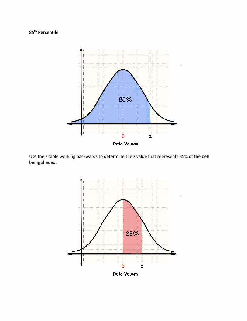
85th Percentile

Use the z table working backwards to determine the z value that represents 35% of the bell being shaded.

0 z

TABLE A-2 Standard Normal (z) Distribution

z .00 .01 .02 .03 .04 .05 .06 .07 .08 .09

0.0 .0000 .0040 .0080 .0120 .0160 .0199 .0239 .0279 .0319 .03590.1 .0398 .0438 .0478 .0517 .0557 .0596 .0636 .0675 .0714 .07530.2 .0793 .0832 .0871 .0910 .0948 .0987 .1026 .1064 .1103 .11410.3 .1179 .1217 .1255 .1293 .1331 .1368 .1406 .1443 .1480 .15170.4 .1554 .1591 .1628 .1664 .1700 .1736 .1772 .1808 .1844 .1879

0.5 .1915 .1950 .1985 .2019 .2054 .2088 .2123 .2157 .2190 .22240.6 .2257 .2291 .2324 .2357 .2389 .2422 .2454 .2486 .2517 .25490.7 .2580 .2611 .2642 .2673 .2704 .2734 .2764 .2794 .2823 .28520.8 .2881 .2910 .2939 .2967 .2995 .3023 .3051 .3078 .3106 .31330.9 .3159 .3186 .3212 .3238 .3264 .3289 .3315 .3340 .3365 .3389

1.0 .3413 .3438 .3461 .3485 .3508 .3531 .3554 .3577 .3599 .36211.1 .3643 .3665 .3686 .3708 .3729 .3749 .3770 .3790 .3810 .38301.2 .3849 .3869 .3888 .3907 .3925 .3944 .3962 .3980 .3997 .40151.3 .4032 .4049 .4066 .4082 .4099 .4115 .4131 .4147 .4162 .41771.4 .4192 .4207 .4222 .4236 .4251 .4265 .4279 .4292 .4306 .4319

1.5 .4332 .4345 .4357 .4370 .4382 .4394 .4406 .4418 .4429 .44411.6 .4452 .4463 .4474 .4484 .4495 ∗ .4505 .4515 .4525 .4535 .45451.7 .4554 .4564 .4573 .4582 .4591 .4599 .4608 .4616 .4625 .46331.8 .4641 .4649 .4656 .4664 .4671 .4678 .4686 .4693 .4699 .47061.9 .4713 .4719 .4726 .4732 .4738 .4744 .4750 .4756 .4761 .4767

2.0 .4772 .4778 .4783 .4788 .4793 .4798 .4803 .4808 .4812 .48172.1 .4821 .4826 .4830 .4834 .4838 .4842 .4846 .4850 .4854 .48572.2 .4861 .4864 .4868 .4871 .4875 .4878 .4881 .4884 .4887 .48902.3 .4893 .4896 .4898 .4901 .4904 .4906 .4909 .4911 .4913 .49162.4 .4918 .4920 .4922 .4925 .4927 .4929 .4931 .4932 .4934 .4936

2.5 .4938 .4940 .4941 .4943 .4945 .4946 .4948 .4949 ∗ .4951 .49522.6 .4953 .4955 .4956 .4957 .4959 .4960 .4961 .4962 .4963 .49642.7 .4965 .4966 .4967 .4968 .4969 .4970 .4971 .4972 .4973 .49742.8 .4974 .4975 .4976 .4977 .4977 .4978 .4979 .4979 .4980 .49812.9 .4981 .4982 .4982 .4983 .4984 .4984 .4985 .4985 .4986 .4986

3.0 .4987 .4987 .4987 .4988 .4988 .4989 .4989 .4989 .4990 .49903.10 and .4999

higher

NOTE: For values of z above 3.09, use 0.4999 for the area.*Use these common values that result from interpolation:

z score Area

1.645 0.4500

2.575 0.4950

From Frederick C. Mosteller and Robert E. K. Rourke, Sturdy Statistics, 1973, Addison-Wesley Publishing Co., Reading, MA. Reprintedwith permission of Frederick Mosteller.

85th Percentile

TI-83 or TI-84 Plus Finding the z vaue corresponding to a known area. 1. Press 2nd then vars to access DISTR (distributions) menu. 2. Select InvNorm and click enter. 3. Enter the area to the left of the z value, enter the mean 𝜇, enter the standard deviation 𝜎

InvNorm(area to the left,𝝁,𝝈) and press enter

InvNorm (0.85,0,1)

6th Decile

Use the z table working backwards to determine the z value that represents 10% of the bell being shaded.

0 z

TABLE A-2 Standard Normal (z) Distribution

z .00 .01 .02 .03 .04 .05 .06 .07 .08 .09

0.0 .0000 .0040 .0080 .0120 .0160 .0199 .0239 .0279 .0319 .03590.1 .0398 .0438 .0478 .0517 .0557 .0596 .0636 .0675 .0714 .07530.2 .0793 .0832 .0871 .0910 .0948 .0987 .1026 .1064 .1103 .11410.3 .1179 .1217 .1255 .1293 .1331 .1368 .1406 .1443 .1480 .15170.4 .1554 .1591 .1628 .1664 .1700 .1736 .1772 .1808 .1844 .1879

0.5 .1915 .1950 .1985 .2019 .2054 .2088 .2123 .2157 .2190 .22240.6 .2257 .2291 .2324 .2357 .2389 .2422 .2454 .2486 .2517 .25490.7 .2580 .2611 .2642 .2673 .2704 .2734 .2764 .2794 .2823 .28520.8 .2881 .2910 .2939 .2967 .2995 .3023 .3051 .3078 .3106 .31330.9 .3159 .3186 .3212 .3238 .3264 .3289 .3315 .3340 .3365 .3389

1.0 .3413 .3438 .3461 .3485 .3508 .3531 .3554 .3577 .3599 .36211.1 .3643 .3665 .3686 .3708 .3729 .3749 .3770 .3790 .3810 .38301.2 .3849 .3869 .3888 .3907 .3925 .3944 .3962 .3980 .3997 .40151.3 .4032 .4049 .4066 .4082 .4099 .4115 .4131 .4147 .4162 .41771.4 .4192 .4207 .4222 .4236 .4251 .4265 .4279 .4292 .4306 .4319

1.5 .4332 .4345 .4357 .4370 .4382 .4394 .4406 .4418 .4429 .44411.6 .4452 .4463 .4474 .4484 .4495 ∗ .4505 .4515 .4525 .4535 .45451.7 .4554 .4564 .4573 .4582 .4591 .4599 .4608 .4616 .4625 .46331.8 .4641 .4649 .4656 .4664 .4671 .4678 .4686 .4693 .4699 .47061.9 .4713 .4719 .4726 .4732 .4738 .4744 .4750 .4756 .4761 .4767

2.0 .4772 .4778 .4783 .4788 .4793 .4798 .4803 .4808 .4812 .48172.1 .4821 .4826 .4830 .4834 .4838 .4842 .4846 .4850 .4854 .48572.2 .4861 .4864 .4868 .4871 .4875 .4878 .4881 .4884 .4887 .48902.3 .4893 .4896 .4898 .4901 .4904 .4906 .4909 .4911 .4913 .49162.4 .4918 .4920 .4922 .4925 .4927 .4929 .4931 .4932 .4934 .4936

2.5 .4938 .4940 .4941 .4943 .4945 .4946 .4948 .4949 ∗ .4951 .49522.6 .4953 .4955 .4956 .4957 .4959 .4960 .4961 .4962 .4963 .49642.7 .4965 .4966 .4967 .4968 .4969 .4970 .4971 .4972 .4973 .49742.8 .4974 .4975 .4976 .4977 .4977 .4978 .4979 .4979 .4980 .49812.9 .4981 .4982 .4982 .4983 .4984 .4984 .4985 .4985 .4986 .4986

3.0 .4987 .4987 .4987 .4988 .4988 .4989 .4989 .4989 .4990 .49903.10 and .4999

higher

NOTE: For values of z above 3.09, use 0.4999 for the area.*Use these common values that result from interpolation:

z score Area

1.645 0.4500

2.575 0.4950

From Frederick C. Mosteller and Robert E. K. Rourke, Sturdy Statistics, 1973, Addison-Wesley Publishing Co., Reading, MA. Reprintedwith permission of Frederick Mosteller.

6th Decile

TI-83 or TI-84 Plus Finding the z vaue corresponding to a known area. 1. Press 2nd then vars to access DISTR (distributions) menu. 2. Select InvNorm and click enter. 3. Enter the area to the left of the z value, enter the mean 𝜇, enter the standard deviation 𝜎

InvNorm(area to the left,𝝁,𝝈) and press enter

InvNorm (0.60,0,1)

4th Decile

Use the z table working backwards to determine the z value that represents 10% of the bell being shaded along with symmetry to determine a negative z value.

0 z

TABLE A-2 Standard Normal (z) Distribution

z .00 .01 .02 .03 .04 .05 .06 .07 .08 .09

0.0 .0000 .0040 .0080 .0120 .0160 .0199 .0239 .0279 .0319 .03590.1 .0398 .0438 .0478 .0517 .0557 .0596 .0636 .0675 .0714 .07530.2 .0793 .0832 .0871 .0910 .0948 .0987 .1026 .1064 .1103 .11410.3 .1179 .1217 .1255 .1293 .1331 .1368 .1406 .1443 .1480 .15170.4 .1554 .1591 .1628 .1664 .1700 .1736 .1772 .1808 .1844 .1879

0.5 .1915 .1950 .1985 .2019 .2054 .2088 .2123 .2157 .2190 .22240.6 .2257 .2291 .2324 .2357 .2389 .2422 .2454 .2486 .2517 .25490.7 .2580 .2611 .2642 .2673 .2704 .2734 .2764 .2794 .2823 .28520.8 .2881 .2910 .2939 .2967 .2995 .3023 .3051 .3078 .3106 .31330.9 .3159 .3186 .3212 .3238 .3264 .3289 .3315 .3340 .3365 .3389

1.0 .3413 .3438 .3461 .3485 .3508 .3531 .3554 .3577 .3599 .36211.1 .3643 .3665 .3686 .3708 .3729 .3749 .3770 .3790 .3810 .38301.2 .3849 .3869 .3888 .3907 .3925 .3944 .3962 .3980 .3997 .40151.3 .4032 .4049 .4066 .4082 .4099 .4115 .4131 .4147 .4162 .41771.4 .4192 .4207 .4222 .4236 .4251 .4265 .4279 .4292 .4306 .4319

1.5 .4332 .4345 .4357 .4370 .4382 .4394 .4406 .4418 .4429 .44411.6 .4452 .4463 .4474 .4484 .4495 ∗ .4505 .4515 .4525 .4535 .45451.7 .4554 .4564 .4573 .4582 .4591 .4599 .4608 .4616 .4625 .46331.8 .4641 .4649 .4656 .4664 .4671 .4678 .4686 .4693 .4699 .47061.9 .4713 .4719 .4726 .4732 .4738 .4744 .4750 .4756 .4761 .4767

2.0 .4772 .4778 .4783 .4788 .4793 .4798 .4803 .4808 .4812 .48172.1 .4821 .4826 .4830 .4834 .4838 .4842 .4846 .4850 .4854 .48572.2 .4861 .4864 .4868 .4871 .4875 .4878 .4881 .4884 .4887 .48902.3 .4893 .4896 .4898 .4901 .4904 .4906 .4909 .4911 .4913 .49162.4 .4918 .4920 .4922 .4925 .4927 .4929 .4931 .4932 .4934 .4936

2.5 .4938 .4940 .4941 .4943 .4945 .4946 .4948 .4949 ∗ .4951 .49522.6 .4953 .4955 .4956 .4957 .4959 .4960 .4961 .4962 .4963 .49642.7 .4965 .4966 .4967 .4968 .4969 .4970 .4971 .4972 .4973 .49742.8 .4974 .4975 .4976 .4977 .4977 .4978 .4979 .4979 .4980 .49812.9 .4981 .4982 .4982 .4983 .4984 .4984 .4985 .4985 .4986 .4986

3.0 .4987 .4987 .4987 .4988 .4988 .4989 .4989 .4989 .4990 .49903.10 and .4999

higher

NOTE: For values of z above 3.09, use 0.4999 for the area.*Use these common values that result from interpolation:

z score Area

1.645 0.4500

2.575 0.4950

From Frederick C. Mosteller and Robert E. K. Rourke, Sturdy Statistics, 1973, Addison-Wesley Publishing Co., Reading, MA. Reprintedwith permission of Frederick Mosteller.

4th Decile

TI-83 or TI-84 Plus Finding the z vaue corresponding to a known area. 1. Press 2nd then vars to access DISTR (distributions) menu. 2. Select InvNorm and click enter. 3. Enter the area to the left of the z value, enter the mean 𝜇, enter the standard deviation 𝜎

InvNorm(area to the left,𝝁,𝝈) and press enter

InvNorm (0.40,0,1)