Worker Paid Leave Usage Simulation Model User Manual

Worker Paid Leave Usage Simulation Model User Manual January 5, 2021

Worker Paid Leave Usage Simulation Model User Manual

January 5, 2021

Submitted to: United States Department of Labor

Chief Evaluation Office

Attention: Dr. Kuang-chi Chang

Office of the Chief Evaluation Officer 200 Constitution Avenue NW

Washington DC 20005

Submitted by: IMPAQ International, LLC

10420 Little Patuxent Parkway, Suite 300 Columbia, MD 21044

Phone: 443.259.5500 / Fax: 443.367.0477 DUNS: 088656512

www.impaqint.com This document includes information that shall not be disclosed outside the Government and shall not be duplicated, used, or disclosed – in whole or in part – for any purpose other than the conduct of this project. The Government shall have the right to duplicate, use, or disclose the information herein, or any related data to the extent provided in the contract. This restriction does not limit the Government's right to use information contained in this document if it is obtained from another source without restriction. The information subject to this restriction are contained on all pages.

http://www.impaqint.com/

CONTENTS Chapter 1. Introduction .............................................................................................................................. 1

..............................................................................................

................................................................................................

1.1 Background for model development 1

1.2 Model architecture .......................... 2

....................................................................................................

.................................................................................................

1.3 Use and limitations of the model 3

1.4 Model development team contacts 4

Chapter 2. Launching the Model ............................................................................................................... 5

...........................................................................................

..................................................................................................................

....................................................................................................................

2.1 Downloading and installing the model 5

2.2 Hardware requirements 7

2.3 Software requirements 8

2.3.1 Python package requirements ......................................................................................................... 9

2.3.2 R package requirements ............................................................................................................... 10

2.4 Opening the Graphic User Interface (GUI) .................................................................................. 10

2.4.1 Model Execution Option 1: Launching from the Windows executable ....................................... 11

2.4.2 Model Execution Option 2: Launching via a terminal ................................................................. 12

2.4.3 Run Button Validation ................................................................................................................. 12

Chapter 3. Running Simulations ............................................................................................................. 14

3.1 Simulation options ........................................................................................................................ 14

3.1.1 Basic parameters .......................................................................................................................... 14

3.1.1.1 Main GUI panel ............................................................................................................................ 14

3.1.1.2 Program tab .................................................................................................................................. 15

3.1.1.3 Population tab ............................................................................................................................... 17

3.1.1.4 Simulation tab .............................................................................................................................. 17

3.1.2 Compare button ............................................................................................................................ 18

3.1.3 Advanced parameters ................................................................................................................... 19

3.1.3.1 Advanced parameters in main GUI panel .................................................................................... 19

3.1.3.2 Advanced parameters under Program tab .................................................................................... 21

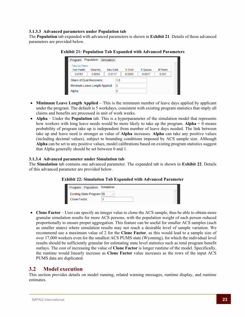
3.1.3.3 Advanced parameters under Population tab ................................................................................. 23

3.1.3.4 Advanced parameter under Simulation tab .................................................................................. 23

3.2 Model execution ........................................................................................................................... 23

3.2.1 Running the model ....................................................................................................................... 24

3.2.2 Warning messages ........................................................................................................................ 24

3.2.3 Runtime display............................................................................................................................ 25

3.2.4 Runtime estimates ........................................................................................................................ 25

Chapter 4. Interpreting Simulation Results ........................................................................................... 26

4.1 Simulation output ......................................................................................................................... 26

4.1.1 Summary tab ................................................................................................................................ 26

4.1.2 Benefit financing tab .................................................................................................................... 27

4.1.3 Population analysis tab ................................................................................................................. 29

4.2 Output folder ................................................................................................................................ 32

APPENDIX ................................................................................................................................................ 34

TABLE OF EXHIBITS Exhibit 1: Architecture of the Worker PLUS Model .................................................................................... 3 Exhibit 2: Model Configurations Affecting ACS File Download, State of Work and Year ......................... 6 Exhibit 3: Summary of Downloaded Folders after Unzipping, by Model Execution Option and ACS File Download Option .......................................................................................................................................... 6 Exhibit 4: Summary of Disk Space Requirements ........................................................................................ 8 Exhibit 5: Using PowerShell to Navigate to the Folder Hosting Microsimulator.py ................................... 9 Exhibit 6: List of Additional Python Packages Required after Installing Python ......................................... 9 Exhibit 7: List of Additional R Packages Required after Installing R ........................................................ 10 Exhibit 8: Launching the Model from Executable ...................................................................................... 11 Exhibit 9: Windows Command Line Window Displayed during Model Launching via Executable ......... 12 Exhibit 10: Launching the Model from Terminal ....................................................................................... 13 Exhibit 11: Main GUI Panel, with GUI Window Expanded Showing Full File and Directory Paths ........ 14 Exhibit 12: Basic Parameters under Program Tab ...................................................................................... 15 Exhibit 13: Configuring Wage Replacement Parameters under Wage Bracket-Based Replacement Type .................................................................................................................................................................... 16 Exhibit 14: Basic Parameters under Population Tab ................................................................................... 17 Exhibit 15: Basic Parameter under Simulation Tab .................................................................................... 18 Exhibit 16: Compare Button to Enable Parallel Simulations ...................................................................... 19 Exhibit 17: Main GUI Panel Expanded with Advanced Parameters .......................................................... 20 Exhibit 18: Underlying Python and R Packages for All Simulation Methods ............................................ 20 Exhibit 19: Specifying Rscript Path after Setting Engine Type as R .......................................................... 21 Exhibit 20: Program Tab Expanded with Advanced Parameters ................................................................ 22 Exhibit 21: Population Tab Expanded with Advanced Parameters ............................................................ 23 Exhibit 22: Simulation Tab Expanded with Advanced Parameter .............................................................. 23 Exhibit 23: Warning Message after Clicking Run Button, Confirming Availability of ACS Data Files .. 24 Exhibit 24: Warning Message after Clicking Run Button, Runtime Implication for Running Model for All States ........................................................................................................................................................... 24 Exhibit 25: Runtime Display Window ........................................................................................................ 25 Exhibit 26: Summary Tab, Program Benefit Costs ..................................................................................... 26 Exhibit 27: Summary Tab, Leave Takers under Program ........................................................................... 27 Exhibit 28: Benefit Financing Tab, Population-Level Estimates and Tax Revenue by Wage Group ........ 27 Exhibit 29: Benefit Financing Tab, Tax Revenue by Gender ..................................................................... 28 Exhibit 30: Benefit Financing Tab, Tax Revenue by Age Group ............................................................... 28 Exhibit 31: Benefit Financing Tab, Tax Revenue Class of Worker ........................................................... 28 Exhibit 32: Updating Benefit Financing Parameters .................................................................................. 29 Exhibit 33: Population Analysis Tab, with Graphs Updated by an Example Subgroup, Number of Leave Takers under Program by Leave Length ..................................................................................................... 30 Exhibit 34: Population Analysis Tab, Number of Leave Takers Regardless of Program Participation by Additional Leave Length due to Program Implementation ......................................................................... 31 Exhibit 35: Population Analysis Tab, Number of Leave Takers under Program by Leave Length, Comparison Simulation .............................................................................................................................. 31 Exhibit 36: Population Analysis Tab, Number of Leave Takers Regardless of Program Participation by Additional Leave Length due to Program Implementation, Comparison Simulation ................................ 31 Exhibit 37: Files in the Output Directory .................................................................................................... 33

1 IMPAQ International

Chapter 1. Introduction

1.1 Background for model development

The Family and Medical Leave Act (FMLA) has provided up to 12 weeks of job-protected unpaid leave to eligible U.S. workers since 1993.1 While the FMLA has increased access to leave among eligible workers, the scale of the program is still limited. To qualify, workers must have worked at least 1,250 hours over the past 12 months for the same employer, and the employer must have at least 50 employees within 75 miles of the work site.2,3 About 45% of workers do not meet these requirements. The unpaid nature of the FMLA leaves about 50 million U.S. workers without access to paid sick days, and many workers lack sufficient paid time off for their own or family members’ medical needs. Only 39% have access to short-term disability insurance that provides cash benefits for non-work-related medical conditions, including childbirth, and only 15% of workers have access to paid leave to care for family members.4 Even among these workers, the low wage replacement rates still render leave time unaffordable for many. To address the gap in paid leave coverage for workers, paid family and medical leave programs have received considerable support from states and municipalities, and some jurisdictions have moved forward on implementing programs for paid family leave. California enacted paid family leave legislation in 2002, New Jersey in 2008, Rhode Island in 2013, New York in 2016, the District of Columbia in 2017, Washington in 2017, Massachusetts in 2018, and Colorado in 2020.5 To facilitate the understanding of the impacts of different policy alternatives on leave-taking behaviors and costs, the Chief Evaluation Office at the U.S. Department of Labor (DOL) has contracted with IMPAQ International (IMPAQ) and the Institute for Women’s Policy Research (IWPR) to develop the Worker Paid Leave Usage Simulation (Worker PLUS) model, an open-source microsimulation tool based on public microdata and predictive modeling. This simulation tool offers a convenient and data-intensive approach for federal, state, and local policy makers and other decision makers to (i) simulate different scenarios of a paid leave program, (ii) estimate the program benefit costs, (iii) estimate payroll tax revenue needed to fund the program benefit costs, (iv) perform population analyses for program participants and eligible workers by focusing on their leave-taking behavior, and (v) compare simulation results across different sets of model parameter input. The simulation engines are developed in both Python and R, two of the most popular open-source programming languages, and the model code is fully transparent and publicly available to facilitate future data updates and model development. The simulation results have also been fully validated between Python and R and against existing state program data.

1 Congress (1993). Family and Medical Leave Act of 1993. 130th Congress. January 5. Washington, DC. 2 Jorgensen, H., & Appelbaum, E. (2014). Documenting the need for a national paid family and medical leave program: Evidence from the 2012 FMLA survey. Center for Economic Policy and Research, Washington, DC. 3 Klerman, J. A., Daley, K., and Pozniak, A. (2012). Family and medical leave in 2012: Technical report. Cambridge, MA: Abt Associates Inc. 4 Acosta and Wiatrowski (2017). National Compensation Survey: Employee Benefits in the United States, March 2017. September. Bulletin 2787. U.S. Bureau of Labor Statistics. 5 Donovan, S. A. (2019). Paid family leave in the United States (CRS Report R44835). Washington, DC. Congressional Research Service, and The New York Times (2020). Colorado Proposition 118 Election Results: Establish Paid Medical and Family Leave. Retrieved from https://www.nytimes.com/interactive/2020/11/03/us/elections/results-colorado-proposition-118-establish-paid-medical-and-family-leave.html?auth=login-google

https://www.nytimes.com/interactive/2020/11/03/us/elections/results-colorado-proposition-118-establish-paid-medical-and-family-leave.html?auth=login-google

https://www.nytimes.com/interactive/2020/11/03/us/elections/results-colorado-proposition-118-establish-paid-medical-and-family-leave.html?auth=login-google


1.2 Model architecture

The Worker PLUS model uses the DOL FMLA Employee Survey public microdata to train models for individual-level leave needs and behaviors. With user-supplied paid leave program parameters (such as eligibility rules), the model then simulates specific leave-taking behavior and outcomes (including number of leaves, leave lengths, benefit levels, and benefit eligibility) with individual workers in a state using data from the five-year American Community Survey (ACS) Public Use Microdata Sample (PUMS). The model outputs a post-simulation ACS PUMS state sample, which allows users to analyze leave benefits of the given paid leave program for individuals, subgroups, and the population. The Worker PLUS model offers a graphical user interface for accessibility to non-technical users. It also offers a benefit financing module to help calculate how taxes and other financing methods can be used to offset program benefit and administrative costs. The post-simulation ACS sample can be used for many different kinds of analyses, including population analyses, policy simulations, counterfactual simulations, cost analyses, and sandbox capabilities.

The Worker PLUS model was developed as an evolutionary iteration of the Paid Family and Medical Leave Simulator Model developed by Albelda and Clayton-Matthews (the ACM model).6 The ACM model was initially developed in 2007 and has been revised and updated several times since 2015, with the most recent update occurring in September 2017. The Worker PLUS model has enhanced the ACM model by offering the following features: (i) a more rigorous simulation engine with leave lengths simulated based on leave reasons and take-up rates calibrated against program administrative statistics; (ii) improved structures of model output and an easy-to-use graphical user interface; (iii) shorter runtime; (iv) simultaneous comparisons across multiple simulations under a single execution of the model; (v) options of both traditional and machine learning simulation methods; and (vi) open-source coding in both Python and R, two of the most popular modern languages among data scientists, that allows for greater transparency and flexibility to users and researchers.

The simulation model runs through the broad steps below to simulate leave taking among the ACS population based on user input of simulation method, program eligibility rules, program benefits, and population characteristics. For each observation in the population:

1. Predictive models are trained using FMLA Employee Survey public microdata. In particular: a. The models are trained using the classifier specified by the user. Classifier options include

Logistic Regression GLM (i.e., the traditional logistic regression from the general linear model family), Logistic Regression Regularized, Ridge Classifier, K Nearest Neighbor, Naïve Bayes, Support Vector Machine, Random Forest, and XGBoost.

b. Feature variables are those that are available from both the FMLA and ACS microdata files, including age; marital status; educational attainment; race; family income; wage; work hours per week; occupation and industry codes as specified by the Census Current Population Survey; eligibility for FMLA coverage (the existing unpaid leave coverage); and statuses of childbearing, living with elderly dependents, hourly paid, labor union membership, nonprofit organization employment, and government employment,

2. Leave-taking status is simulated using one of the trained predictive models from Step 1, as specified by the model user.

3. Leave length in absence of any state paid leave program is simulated.

6 Clayton-Matthews, Alan, and Randy Albelda (2017). Description of the Albelda Clayton-Matthews/IWPR 2017 Paid Family and Medical Leave Simulator Model.


4. Maximum length of leave needed is simulated. 5. Based on the wage replacement rates of the employer and the state program as specified by the

model user through a set of program parameters, the leave length taken in the presence of the state program is determined by interpolating a value using leave lengths obtained from between Steps 1 and 2.

6. Based on the relative levels of wage replacement rates between the employer and the state program, length of leave covered by the program (as a length up to the leave length simulated in Step 3) is determined.

7. Program participation is randomly determined based on user input values for uptake for each leave type.

8. The above steps result in a post-simulation ACS state sample with leave lengths and program benefits received included as individual-level data elements. Then program outlays, tax revenues, total leave lengths, etc., can be computed as population aggregates. Subpopulation analysis such as the low-wage worker analysis done in this paper can also be performed.

Exhibit 1 provides a flow chart for the architecture of the Worker PLUS model.

Exhibit 1: Architecture of the Worker PLUS Model

1.3 Use and limitations of the model

The Worker PLUS model attempts to predict a set of complex leave-taking behaviors, based on a limited set of variables available in public data. In general, the model results should provide draft estimates for feasibility study, early-stage planning, and preliminary impact evaluation of a paid leave program at an aggregate level. Users should take caution when extrapolating from individual-level leave taking. Notably, there is a lack of some relevant variables in the FMLA and ACS datasets that are associated with leave-taking behavior, including health status, time preference, nature and urgency of medical needs, and job security of workers. The predictive performance of the model at the individual level is affected by the absence of these variables as predictors. To facilitate future model development and improvement should more and better data sources become available, the model features a transparent and modularized code repository that provides open access to model users, policy analysts, programmers, and researchers.


In addition, user discretion is needed for configuring model parameters to approximate the program under consideration. The model provides a long list of program and population parameters, but the list cannot capture all rules that ever have been or will be adopted by existing or future paid leave programs. It is expected that even with a close approximation of program and population parameters to real life, the results (e.g., program benefit outlays) may be different from actual data. In the model graphical user interface, some default parameters have been programmed in, but it is important that users carefully follow this user manual to understand the definition and use of all parameters when making any changes to them.

).

Finally, the model features an administrative budget financing (ABF) module that allows estimation of payroll tax revenues based on user-supplied parameters such as payroll tax rates and maximum taxable income. While this module is a convenient tool that provides preliminary estimates for benefit financing aspects of a paid leave program, it is constrained by the limitations in compensation data available in public data sources. For example, the ABF module can only be used for estimating payroll tax revenues and does not capture the full complexities of all possible taxable sources of income if such benefit financing configurations need to be considered. In addition, the ABF estimates are subject to measurement error in ACS job and wage data, including misreporting, top-coding, and missing values.7,8,9 As demonstrated in a separate issue brief that reports the benchmarking results of the ABF module, the module is found to underestimate actual state tax revenues by about 15% based on actual program tax revenue data published by California, New Jersey, and Rhode Island during 2014–2018. 10 Besides the above-mentioned measurement errors, other sources that cause the underestimation may include possible negative annual values of income that resulted from business losses and lack of information for identifying workers who voluntarily opt into program coverage. These findings suggest that the ABF module should be treated as a lower bound estimate of payroll tax revenues.

1.4 Model development team contacts The Worker PLUS model is developed by IMPAQ International and the IWPR under a contract with the DOL Chief Evaluation Office. Questions about technical support should be directed to Dr. Minh Huynh ([email protected]) and Dr. Chris Li Zhang ([email protected]

7 Baum-Snow, Nathaniel, and Derek Neal. "Mismeasurement of usual hours worked in the census and ACS." Economics Letters 102.1 (2009): 39–41. 8 Rothbaum, Jonathan. "Comparing Income Aggregates: How do the CPS and ACS Match the National Income and Product Accounts, 2007–2012." U.S. Census Bureau SEHSD Working Paper 1 (2015). 9 Crimi, Nicole, and William Eddy. "Top-Coding and Public Use Microdata Samples from the U.S. Census Bureau." Journal of Privacy and Confidentiality 6.2 (2014). 10 See IMPAQ (2021). Worker Paid Leave Usage Simulation (Worker PLUS) Model Issue Brief: Benchmarking Results of the Administrative Benefit Financing Module’s Payroll Tax Revenue Estimates.

mailto:[email protected]

mailto:[email protected]


Chapter 2. Launching the Model

This chapter provides details on model downloading and installation, requirements on software and hardware, and model launching via the graphic user interface (GUI). When users’ manual configuration

and installation are needed, a step-by-step guide is provided and highlighted by the icon.

2.1 Downloading and installing the model

The Worker PLUS model is initially uploaded by IMPAQ to a secured SFTP repository that contains the following files and folders:

• file: docs.zip • file: microsim-dev.zip • file: Microsimulator.zip • folder: acs_all_options, which contains

file: 2016_pow.zip file: 2016_res.zip file: 2017_pow.zip file: 2017_res.zip file: 2018_pow.zip file: 2018_res.zip

• folder: acs_default, which contains file: 2018.zip

After obtaining access to the repository, and confirming that the repository contains the above files and folders, the following steps should be followed for model downloading and installation:

1. Download docs.zip, which contains the user manual and data dictionary files. 2. Users should choose one of the following two options to run the model

• Model Execution Option 1: Run a Python model from a stand-alone Windows executable (.exe file). This option is suitable for users without Python installed on the machine. Users choosing this option should download Microsimulator.zip.

• Model Execution Option 2: Run a Python or R model from a terminal such as Windows Command Prompt or PowerShell. This option is suitable for users with either Python or R installed on the machine, and users who are more experienced with open-source programming. Users choosing this option should microsim-dev.zip

3. Users should choose one of the following two options to download the Census American Community Survey (ACS) five-year public use microsample (PUMS) data files, which are one of the required input data sources for the model.

• ACS File Download Option A: Download the ZIP file in the folder acs_default in the SFTP repository. This will download the ACS PUMS data files that will work only for the default option of the Worker PLUS model’s configurations of Year and State of Work. The default option is to use 2014 – 2018 ACS PUMS state files based on workers’ state of work. These are the latest ACS PUMS files as of October 2020. Defining workers’ state as state of work (rather than state of residence) is the common practice of existing state paid leave programs. For ACS File Download Option A, the ZIP file has a size of 1.88 GB, and the unzipped folder has a total file size of 11.4 GB.


• ACS File Download Option B: Download all ZIP files in the folder acs_all_options in the SFTP repository. This will download the ACS PUMS data files that will work for all options (including the default option) of the Worker PLUS model’s configurations of Year and State of Work. Options for Year (the ending year of five-year ACS PUMS sample period) include 2016, 2017, and 2018. Options for State of Work include True (box checked) and False (box unchecked). These options are illustrated in Exhibit 2, which illustrates the checkbox State of Work and dropdown menu Year in the model graphic user interface (GUI). For ACS File Download Option B, the ZIP file has a size of 13.2 GB, and the unzipped folder has a total file size of 81.5 GB. The additional ACS files available from the ACS File Download Option B allow users to perform simulations for evaluating programs using historical data, or exploring difference in simulation outcomes using different definitions of workers’ state. Users also need the ACS PUMS 2012 – 2016 data files to benchmark the Worker PLUS model against the ACM model, an exercise explained in more details in a separate issue brief accompanying the Worker PLUS model materials.11 The ACS File Download Option A is recommended for saving local disk space if users do not need to perform these simulations.

Exhibit 2: Model Configurations Affecting ACS File Download, State of Work and Year

After the files are downloaded, users should follow steps below to place the ACS PUMS data files.

1. Unzip all ZIP folders downloaded. This should result in the following folders based on the Model Execution Option and ACS File Download Option chosen above:

Exhibit 3: Summary of Downloaded Folders after Unzipping, by Model Execution Option and ACS File Download Option

Model Execution Option 1 Model Execution Option 2

ACS File Download Option A

docs Microsimulator 2018

docs microsim-dev 2018

11 See IMPAQ (2021). Worker Paid Leave Usage Simulation (Worker PLUS) Model Issue Brief: A Benchmarking Study of the Worker PLUS Model Results.


ACS File Download Option B

docs Microsimulator 2016_res 2016_pow 2017_res 2017_pow 2018_res 2018_pow

docs microsim-dev 2016_res 2016_pow 2017_res 2017_pow 2018_res 2018_pow

2. For ACS File Download Option A (the two scenarios in top row of table above): Locate thesubfolder Microsimulator/data/acs, or microsim-dev/data/acs. Place the folder ‘2018’ in thesubfolder.

3. For ACS File Download Option B (the two scenarios in bottom row of table above): Locate thesubfolder Microsimulator/data/acs, or microsim-dev/data/acs. Create an empty folder ‘2018’ in thesubfolder. Then move pow_household_files, pow_person_files in the folder 2018_pow to the newempty folder ‘2018’, and move household_files, person_files in the folder 2018_res to the samefolder ‘2018’. For example, this will result in the following directory paths

a. Microsimulator/data/acs/2018/pow_household_files.b. Microsimulator/data/acs/2018/pow_person_files.c. Microsimulator/data/acs/2018/household_files.d. Microsimulator/data/acs/2018/person_files.

Repeat this step for 2016 and 2017 files.

4. Alternatively, users can also create an empty parent folder anywhere in local machine to store ACSfiles, replacing Microsimulator/data/acs or microsim-dev/data/acs. Users, however, will need tonavigate to this customized parent folder file path in the model graphic user interface (GUI).

5. User can place the docs folder at any desired local directory for reference needs. We recommendplacing docs directly under the folder Microsimulator or microsim-dev.

2.2 Hardware requirements

The model has been tested on mainstream workplace and home computers with Intel i5 and i7 multicore processors, resulting in manageable runtime (within an hour) even for large states from the American Community Survey (ACS) 5-year public use microdata sample (PUMS) such as California. Runtime is less than 5 minutes for small states such as Rhode Island. Minimum RAM tested is 8GB which is sufficient to handle large ACS states (California data is less than 2GB), although we recommend 16GB RAM or higher for better runtime performance.

The requirement on disk space varies based on user choice of ACS File Download Option (either Option A or Option B) as described in Section 2.1. Exhibit 4 provides a summary of disk space requirements for each component of model files as well as the disk space required for all model files. The total file size is primarily affected by user choice of the ACS File Download Option, which is ultimately dependent upon their analytical needs. If the model is used mainly for prospective program feasibility study, planning, or simulation-based population analysis, then ACS files from Option A should be sufficient. These analyses should be based on more recent ACS data files and should focus on common practice of existing programs on defining workers’ state using state of workplace. If users intend to use the model for validation against historical program statistics or for exploring the alternative definition of workers’ state using state of residence, then Option B would be preferred. This option requires about 70GB additional disk space.


The file sizes of the other two input datasets, the Family and Medical Leave Act (FMLA) Employee Survey and the Current Population Survey (CPS) data sets (which are used to impute a few missing variables in the ACS PUMS) are about 60MB in file size, which has limited impact on the hardware requirements.

Exhibit 4: Summary of Disk Space Requirements

ACS File Download Option A (for model uses with default ACS setting only:

Year = 2018 and State of Work = True)

ACS File Download Option B (for model uses with all ACS settings:

Year = 2016, 2017, or 2018, and State of Work = True or False)

Model code files (without Windows executable) 177MB 177MB

DOL FMLA Employee Survey data files 40MB 40MB

Census CPS data files 41MB 41MB ACS data files 11.4GB 81.5GB

Model documentation files <1MB <1MB Disk space required for

all model files 11.7GB 81.8GB

Note: With the Windows executable, model code total file size will be 325MB, hence an additional 148MB of disk space is required. Disk space required for all model files would then be 11.8GB and 82.0GB for the two ACS File Download Options respectively.

2.3 Software requirements

While the Worker PLUS model provides two simulation engines programmed respectively in Python and R, both simulation engines are ported to the same graphic user interface (GUI) programmed in Python using the Python package tkinter. The GUI also gathers data output from the simulation engine to produce the visualization output (e.g. bar charts and histograms) and final model output files (e.g. summary of program benefit outlays), and these steps require dependencies on other Python packages. Therefore, regardless of users’ preference on simulation engine (Python or R), Python is always required for launching the model.

Current Python simulation engine is coded in Python 3.7, which is also the minimum version required for model execution. Users should follow guidelines in https://www.python.org/downloads/ to install or update the Python programming language.

After installing Python, the exact set of packages to be installed depends on the simulation engine that the user would like to use, and the Model Execution Option chosen in Section 2.1. Specifically:

For users who would like to use the Python simulation engine:

• Users who choose Model Execution Option 1 (using the Windows executable in the folder Microsimulator) should skip Section 2.3 and directly proceed to Section 2.4 to open the GUI.

• Users who choose Model Execution Option 2 (using the source code in the folder microsim-dev) should follow Section 2.3.1 to ensure that all the required Python packages are installed.

For users who would like to use the R simulation engine:

• Users who choose the Model Execution Option 1 (using the Windows executable in the folder Microsimulator) should:

o Skip Section 2.3.1, as the Python packages needed for the GUI has been compiled in the executable

https://www.python.org/downloads/


o Follow Section 2.3.2 to ensure that all the required R packages are installed, ando Proceed to Section 2.4 to open the GUI.

• Users who choose the Model Execution Option 2 (using the source code in the folder microsim-dev) should follow the entire Section 2.3 to ensure that the required Python and R packages areinstalled.

2.3.1 Python package requirements

As described above, the Python packages listed in this section should be installed by users who choose Model Execution Option 2 (using the source code in the folder microsim-dev), regardless of the choice of simulation engine.

After installing Python, users can quickly install the additional needed packages by following these steps:

1. Open the Windows Command Prompt or PowerShell.2. Navigate to the directory that hosts the file Microsimulator.py. For example, if the file

Microsimulator.py is located in E:\workfiles\Microsimulation\microsim, then users should typecd E:\workfiles\Microsimulation\microsim

and then hit Enter to navigate to this directory. This step is illustrated in Exhibit 5.

Exhibit 5: Using PowerShell to Navigate to the Folder Hosting Microsimulator.py

3. Type the command pip install –r requirements.txt and then hit enter.

Users who already have any of the required packages installed but are unable to update them to the latest versions can use the command pip install <package>. Users should replace <package> with one of the packages listed in Exhibit 6, and repeat executing the command pip install <package> for all these packages.

Exhibit 6: List of Additional Python Packages Required after Installing Python

Python Package Python Package cycler==0.10.0 pyparsing==2.4.5

kiwisolver==1.1.0 python-dateutil==2.8.1 matplotlib==2.2.3 pytz==2019.3

mord==0.5 scikit-learn==0.20.1 numpy==1.17.4 scipy==1.3.3 pandas==0.23.0 six==1.13.0

xgboost==1.0.2

Advanced Python users may wish to use a separate virtual environment for Python package management for the model. The Appendix provides details on Python package installation in a virtual environment.


2.3.2 R package requirements

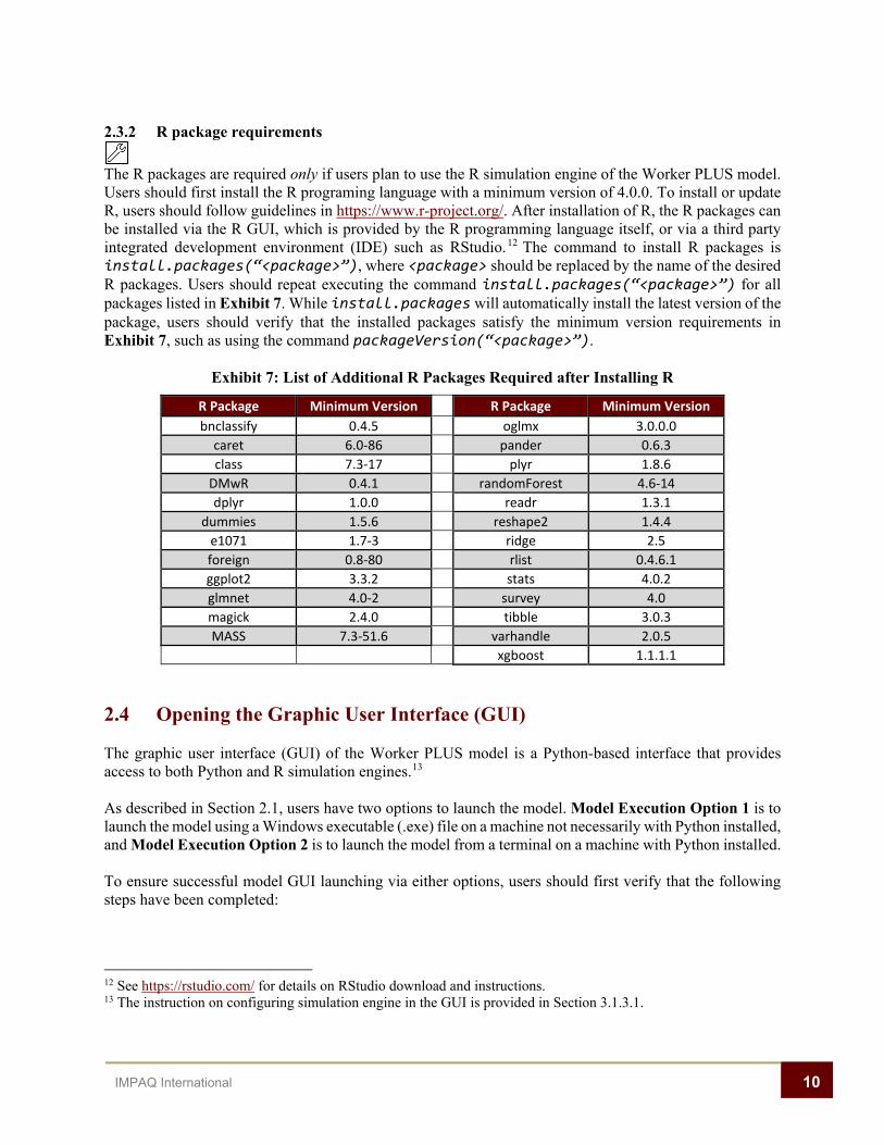
The R packages are required only if users plan to use the R simulation engine of the Worker PLUS model. Users should first install the R programing language with a minimum version of 4.0.0. To install or update R, users should follow guidelines in https://www.r-project.org/. After installation of R, the R packages can be installed via the R GUI, which is provided by the R programming language itself, or via a third party integrated development environment (IDE) such as RStudio.12 The command to install R packages is install.packages(“<package>”), where <package> should be replaced by the name of the desired R packages. Users should repeat executing the command install.packages(“<package>”) for all packages listed in Exhibit 7. While install.packages will automatically install the latest version of the package, users should verify that the installed packages satisfy the minimum version requirements in Exhibit 7, such as using the command packageVersion(“<package>”).

Exhibit 7: List of Additional R Packages Required after Installing R

R Package Minimum Version R Package Minimum Version bnclassify 0.4.5 oglmx 3.0.0.0

caret 6.0-86 pander 0.6.3 class 7.3-17 plyr 1.8.6

DMwR 0.4.1 randomForest 4.6-14 dplyr 1.0.0 readr 1.3.1

dummies 1.5.6 reshape2 1.4.4 e1071 1.7-3 ridge 2.5 foreign 0.8-80 rlist 0.4.6.1 ggplot2 3.3.2 stats 4.0.2 glmnet 4.0-2 survey 4.0 magick 2.4.0 tibble 3.0.3 MASS 7.3-51.6 varhandle 2.0.5

xgboost 1.1.1.1

2.4 Opening the Graphic User Interface (GUI)

The graphic user interface (GUI) of the Worker PLUS model is a Python-based interface that provides access to both Python and R simulation engines.13

As described in Section 2.1, users have two options to launch the model. Model Execution Option 1 is to launch the model using a Windows executable (.exe) file on a machine not necessarily with Python installed, and Model Execution Option 2 is to launch the model from a terminal on a machine with Python installed.

To ensure successful model GUI launching via either options, users should first verify that the following steps have been completed:

12 See https://rstudio.com/ for details on RStudio download and instructions. 13 The instruction on configuring simulation engine in the GUI is provided in Section 3.1.3.1.

https://www.r-project.org/

https://rstudio.com/


• All model code files have been successfully downloaded and unzipped into the model code folder (either Microsimulator or microsim-dev), as described in Section 2.1

• The ACS data files have been properly placed, as described in Section 2.1 • The hardware and software requirements are satisfied, as described in Sections 2.2 and 2.3

After above verifications, the GUI can be launched as below:

2.4.1 Model Execution Option 1: Launching from the Windows executable

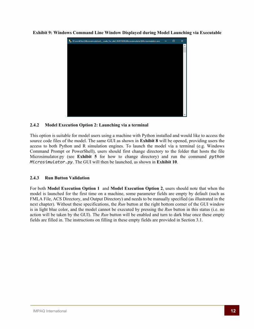
This option is particularly suitable for users using a machine without Python installed, by providing a Windows executable (.exe file). The Windows executable is contained in the folder ‘Microsimulator’. Users should locate the file Microsimulator.exe in the folder, and double click this file to launch the model GUI, as shown in Exhibit 8. On some machines, an empty Windows Command Line window may show up for up to two minutes before the GUI launches, as shown in Exhibit 9. The presence of the Windows Command Line window indicates that the GUI launching is in progress, and user should wait until it disappears and the GUI window appears as in Exhibit 8. Users should not close the Windows Command Line window during the waiting time, as this will terminate the GUI launching process.

Upon double clicking Microsimulator.exe, on some machines the Windows system might display a warning message asking for user permission to run the executable. Users should choose More Info and then choose Run Anyway to continue the launching process. The warning message may occur on Windows machines with stricter security settings due to the current non-certified status of this open-source executable program. Users should have Administrator access of the Windows operating system to bypass this warning. Users without Administrator access should contact their IT staff to bypass this warning.

Exhibit 8: Launching the Model from Executable


Exhibit 9: Windows Command Line Window Displayed during Model Launching via Executable

2.4.2 Model Execution Option 2: Launching via a terminal

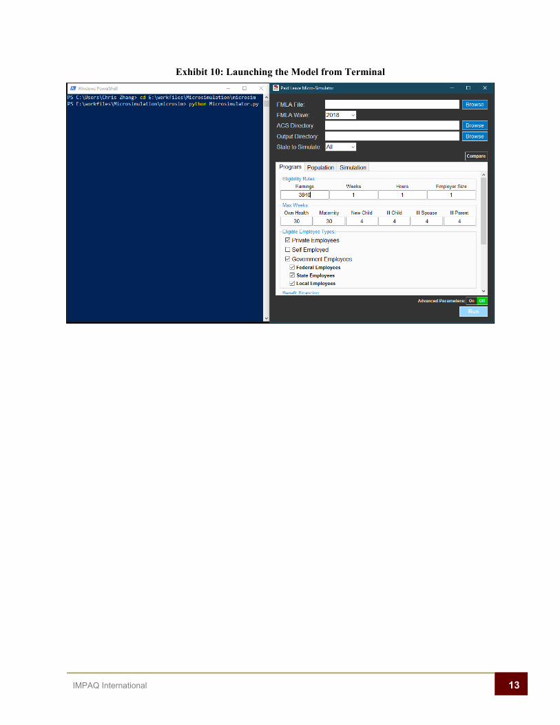
This option is suitable for model users using a machine with Python installed and would like to access the source code files of the model. The same GUI as shown in Exhibit 8 will be opened, providing users the access to both Python and R simulation engines. To launch the model via a terminal (e.g. Windows Command Prompt or PowerShell), users should first change directory to the folder that hosts the file Microsimulator.py (see Exhibit 5 for how to change directory) and run the command python Microsimulator.py. The GUI will then be launched, as shown in Exhibit 10.

2.4.3 Run Button Validation

For both Model Execution Option 1 and Model Execution Option 2, users should note that when the model is launched for the first time on a machine, some parameter fields are empty by default (such as FMLA File, ACS Directory, and Output Directory) and needs to be manually specified (as illustrated in the next chapter). Without these specifications, the Run button at the right bottom corner of the GUI window is in light blue color, and the model cannot be executed by pressing the Run button in this status (i.e. no action will be taken by the GUI). The Run button will be enabled and turn to dark blue once these empty fields are filled in. The instructions on filling in these empty fields are provided in Section 3.1.


Exhibit 10: Launching the Model from Terminal


CHAPTER 3. RUNNING SIMULATIONS 3.1 Simulation options Once the graphic user interface (GUI) is displayed as shown in Exhibit 8 or Exhibit 10. The next steps are specifying a set of model parameters, before executing the simulation.

3.1.1 Basic parameters As shown in Exhibit 8 and Exhibit 10, there is an Advanced Parameters switch at the right bottom corner of the GUI window. The switch is at “Off” status when the model is launched for the first time, and the GUI would only display the basic parameters for the model. The next few subsections will focus on these basic parameters. The advanced parameters (enabled to turning the switch to “On”) will be discussed in Section 3.1.3.

3.1.1.1 Main GUI panel The main GUI panel is the upper area of the GUI window with a dark background, as shown in Exhibit 11 which also expands the GUI window horizontally to illustrate the full file and directory paths after the basic parameter fields have been filled in.

Exhibit 11: Main GUI Panel, with GUI Window Expanded Showing Full File and Directory Paths

The basic parameters in the main GUI panel includes the following: • FMLA File – File path to the DOL FMLA Employee Survey data file. Users can use the file

FMLA_2018_Employee_PUF.csv located at ./data/fmla_2018/. To select this file, users should use the Browse button on the right to navigate to and select the CSV file. User should verify that after selection this field displays the full file path to the CSV file, including the “.csv” extension.

• FMLA Wave – Wave year of the FMLA dataset. Users should specify either 2012 or 2018, the only two values allowed, as these are the only two waves of DOL FMLA Employee Survey programmed as model input. Users should also verify that the wave year is consistent with the file path specified in FMLA File.

• ACS Directory – Directory of ACS data files. If users have followed instructions in Section 2.1 of this manual by placing the downloaded ACS data files in ./data/acs, then user should use the Browse button to navigate to ./data/acs and choose this directory. Alternatively, if users have followed instructions in Section 2.1 and placed the downloaded ACS data files in another local directory (while the structure is


maintained as required, e.g. ./acs/2018/pow_household_files, etc.), users should use the Browse button to navigate to that directory. In either case, upon selection of the directory, user should verify that the field is filled in as a local directory path that ends with “/acs”.

• Output Directory – Directory where output files will be stored upon completion of simulation. Usercan use the built-in output directory ./output, or select an alternative local directory, using the Browsebutton.

• State to Simulate – ACS state PUMS dataset to use as underlying worker population. The dropdownmenu contains 50 states plus DC.

3.1.1.2 Program tab The basic parameters under the Program tab are displayed in Exhibit 12. Details are provided below for each of these parameters.

Exhibit 12: Basic Parameters under Program Tab

• Eligibility Rules – These are minimum requirements on annual earnings (in dollars), number of weeksworked over a year, number of hours worked over a year, and number of employees at workplace for aworker to be eligible to receive leave benefits from the program.


• Max Weeks – These are maximum numbers of weeks within a year for which an eligible worker can receive leave benefits from the program. Users can set different value of maximum number of weeks for each of the six leave reasons. The number of weeks should not exceed 52.

• Eligible Employee Types – At least one of the following employee types needs to be selected using the checkbox. Otherwise, model code will run into a Python IndexError and the simulation will be terminated. Private Employees – If checked, workers working for private business employers will be included

as eligible workers. Government Employees – Type of government employees to be included as eligible workers. If

Government Employee is checked, all three child checkboxes will be automatically checked. Otherwise, users can selectively check zero, one, two, or all of the child checkboxes, including Federal Employees, State Employees, and Local Employees.

Self Employed – If checked, workers under self-employment will be included as eligible workers. • Benefit Financing – These are parameters that configure the payroll tax scheme on eligible workers,

including: Payroll Tax Rate – A positive value (up to 100) representing percentage points of tax rate. Maximum Taxable Earnings – A positive value that places a cap on annual taxable earnings

that are subject to the payroll tax. Apply Benefit Tax – If checked, state income tax will be applied to program benefits received by

program participants State Income Tax Rate – Average state income tax applied to program benefits received by

program participants • Wage Replacement – These are parameters that configure the wage replacement scheme of the

program benefits, including: Wage Replacement Type – The wage replacement can follow one of two types: either Flat or

Wage Bracket-Based. Flat represents a flat rate of wage replacement, regardless the annual wage amount. Wage Bracket-Based represents a set of rates, with each rate applied a corresponding annual wage bracket specified below by users. The Wage Bracket-Based replacement type is particularly useful for program design that has a progressive wage replacement scheme (i.e. a higher wage replacement ratio for lower wage brackets).

Replacement Ratio – Enabled when Wage Replacement Type = Flat. This is the share of wage that would be replaced by program benefits during leave. This ratio should be a positive value between 0 and 1.

Upper Bound – Enabled when Wage Replacement Type = Wage Bracket-Based. Users should provide upper bounds of each annual wage bracket. As shown in Exhibit 13, users can use the green “+” button to add desired number of wage brackets. For each bracket, when the Upper Bound is specified, the Lower Bound for the next bracket will be automatically updated. Users need to specify Upper Bound for all but the top wage bracket, since by definition the Upper Bound for the highest wage bracket will always be infinity.

Wage Replacement – Enabled when Wage Replacement Type = Wage Bracket-Based. Users should provide wage replacement ratio as a value between 0 and 1 (including 0) for each wage bracket specified.

Exhibit 13: Configuring Wage Replacement Parameters under Wage Bracket-Based Replacement Type


• Weekly Benefit Cap – Maximum weekly benefits in dollars. 3.1.1.3 Population tab The basic parameters under the Population tab are displayed in Exhibit 14. Details are provided below for each of these parameters.

Exhibit 14: Basic Parameters under Population Tab

• Take Up Rates – These are program take-up rates for each leave reason among all eligible workers in

the state. Take-up rate is defined as total number of actual leave takers who receive program benefits divided by total number of eligible workers in the state, which is determined by (i) the State of Work checkbox in the main GUI panel, and (ii) the Eligibility Rules and Eligible Employee Types specified under the Program tab. These rates can be set as any value between 0 and 1. The rates displayed in Exhibit 14 are estimated using actual program data in Rhode Island between 2014 and 2018.14

• Share of Dual Receivers – Share of eligible workers who can receive leave benefits simultaneously from both employer and state program, out of all eligible workers who receive any leave pay benefit from employer. This share should be a value between 0 and 1.

3.1.1.4 Simulation tab There is one basic parameter under the Simulation tab, as displayed in Exhibit 15. Details are provided below.

14 The actual program data for programs for California, New Jersey, and Rhode Island are provided in the folder state_program_statistics along with mode code (i.e. under either the folder microsim-dev or Microsimulator).


Exhibit 15: Basic Parameter under Simulation Tab

• Existing State Program – This dropdown menu allows users to use parameters that characterize an existing state program. Available options are CA (representing the state program in California), NJ (representing the state program in New Jersey), and RI (representing the state program in Rhode Island). Upon choosing a state from the dropdown menu, the parameters under the Program tab will be overridden by a set of pre-determined parameters that best represent the leave program of the selected state. Parameters under Population tab will be overridden by a set of empirical estimates, including take-up rates for each leave type estimated from historical state program data.

3.1.2 Compare button The model provides a feature that allow users to run multiple simulations for comparison, with the same parameters in the main GUI panel (i.e. same input of data and state chosen) and different parameters in the Program, Population, and Simulation tabs. The model is programmed such that, during such multiple simulations, the same input data will only be pre-processed once and then used for different simulation scenarios, reducing the total runtime. This runtime-optimized comparison feature can be enabled by the Compare button, as shown in Exhibit 16.


Exhibit 16: Compare Button to Enable Parallel Simulations

After the Compare button is clicked, the Main Simulation button will be added to the left to the Compare button. The Main Simulation represents the original simulation configuration in the GUI. It can be used to return to the Program, Population, and Simulation tabs of the original simulation. Next to the Main Simulation button, a button with a “+” sign will appear. Users can then click the “+” button to add additional comparison simulations to be performed. Exhibit 16 illustrates a case when the “+” button has been pressed once and one comparison simulation has been added. A new button Comparison 1 then appears. When Comparison 1 is highlighted as in Exhibit 16, users can use the Program, Population, and Simulation tabs to specify parameters for the comparison simulation represented by Comparison 1. Likewise, use can use the “+” button to further add up to 4 comparison simulations and configure parameters for the additional comparison simulations accordingly. If a comparison simulation is no longer needed, users can click the “×” button to remove the simulation before running the model. To cancel simulation comparison, users can simply click the green Compare button, which will remove all of the buttons related to the comparison functionalities.

3.1.3 Advanced parameters Besides the basic parameters described above. The model also offers a set of advanced parameters that give users additional control of the simulation. The advanced parameters can be enabled by turning the Advanced Parameters switch to “On”. The Advanced Parameters button is located at the right bottom corner of the GUI Window, above the Run button. After turning on the switch, advanced parameter fields will be activated in the main GUI Panel, Program tab, Population tab, and Simulation tab.

3.1.3.1 Advanced parameters in main GUI panel The main GUI panel expanded with advanced parameters is shown in Exhibit 17. Details of these advanced parameters are provided below.


Exhibit 17: Main GUI Panel Expanded with Advanced Parameters

• State of Work – If checked, state of workers will be determined by state of workplace. If unchecked,state of workers will be determined by state of residence. This parameter is checked as default,following common practice of existing state programs. Users should note that with State of Workunchecked, the model can run only if users chose ACS File Download Option B during modeldownload and installation, as demonstrated in Section 2.1

• Year – This is the ending year of the five-year ACS public use micro sample (PUMS) sample period.The dropdown menu allows values 2016, 2017, 2018. For example, if 2018 is chosen, then the ACSfive-year PUMS 2014 – 2018 data files will be used. Users should note that if Year is set to 2016 or2017, the model can run only if users chose ACS File Download Option B during model downloadand installation, as demonstrated in Section 2.1.

• Simulation Method – This dropdown menu in the GUI main panel allows user to specify the classifierto be used for simulation. The following list of simulation methods are available: Logistic Regression GLM Logistic Regression Regularized Ridge Classifier K Nearest Neighbor Naïve Bayes Support Vector Machine Random Forest, and XGBoost

The Logistic Regression GLM refers to unregularized logistic regression, the traditional method as an instance of the general linear model (GLM) family. All other simulation methods are machine learning classifiers. Exhibit 18 shows the underlying Python and R packages and their versions for the Python and R simulation engines respectively.

Exhibit 18: Underlying Python and R Packages for All Simulation Methods Simulation Method Python Package Version R Package Version Logistic Regression GLM statsmodels 0.12.0 survey 4.0 Logistic Regression Regularized scikit-learn 0.23 glmnet 4.0-2 K Nearest Neighbor (KNN) scikit-learn 0.23 caret 6.0-86 Naïve Bayes scikit-learn 0.23 bnclassify 0.4.5 Random Forest scikit-learn 0.23 randomForest 4.6-14 XGBoost (XGB) xgboost 1.2.0 xgboost 1.1.1.1 Ridge Regression scikit-learn 0.23 ridge 2.5 Support Vector Classifier (SVC) scikit-learn 0.23 e1071 1.7-3


Note: Documentations for the Python statsmodels package specifications and version histories are available from https://www.statsmodels.org/stable/index.html. Documentations for the Python scikit-learn package specifications and version histories are available from https://scikit-learn.org/dev/versions.html. Documentations for the Python xgboost package specifications and version histories are available from https://pypi.org/project/xgboost/#history. All R library documentations and version histories are available from https://rdrr.io/.

• Random seed – If a Random Seed value is provided, then each run of the model will correspond to a machine-generated pseudo-random state represented by the seed value. Using the same seed would allow users to replicate simulation results, provided all other model inputs are the same. Without random seed specified, different simulation results may occur even with all model inputs unchanged, due to the implementation of many random number generator-based algorithms during the simulation process.

• Engine Type – Default value is Python. User can also choose to run the simulation using the R simulation engine, for which the equivalent R simulation code will be used to perform the simulations.

If Engine Type is set to R. An additional input field named Rscript Path will appear under Engine Type, asking the user to specify the file path to the file Rscript.exe, which is the executable needed to execute the R code. Users can use the Browse button on the right to navigate to the local directory that hosts Rscript.exe. This directory is typically [R path]/bin/Rscript.exe, where [R path] is the directory where R is installed. Exhibit 19 illustrates an example of specifying Rscript Path.

Exhibit 19: Specifying Rscript Path after Setting Engine Type as R

Currently, the model does not allow comparison across parallel simulations when Engine Type is set to R, due to compatibility issues between the Python-based GUI and the R programming language. Therefore, the Comparison button will be hidden when Engine Type is set to R.

3.1.3.2 Advanced parameters under Program tab The Program tab expanded with advanced parameters is shown in Exhibit 20. Details of these advanced parameters are provided below.

https://www.statsmodels.org/stable/index.html

https://scikit-learn.org/dev/versions.html

https://pypi.org/project/xgboost/#history

https://rdrr.io/


Exhibit 20: Program Tab Expanded with Advanced Parameters

• Leave Types Allowed – Users can choose to include or exclude leave types (correspondingly denoted by the six leave reasons) allowed by the program. At least one leave type must be checked.

• Wait Period – This is the number of workdays applicants need to wait from approval until receiving benefits. The value should be set as a positive integer.

• Dependency Allowance – If checked, users can specify number of spouse and child dependents and the associated incremental wage replacement ratio offered by the program. For example, in Exhibit 20, the dependency allowance profile means that the program would offer an additional 7% wage replacement for each additional spouse or child dependent of the applicant, up to a maximum of 5 dependents. Users can use the “+” and “–” buttons to control the maximum number of dependents allowed.

• Replacement Ratio (under Dependency Allowance) – These are the incremental wage replacement for each additional dependent specified by the user. The values should be between 0 and 1.

• Recollect – If checked, approved applicants can recollect program benefits accrued during the above-specified waiting period.

• Minimum Leave Length (activated if Recollect is checked) – This is the minimum number of leave days required for benefit recollection. For example, when Recollect is enabled, if Minimum Leave Length is set to 5, the leave length covered by the program must be at least 5 days to enable benefit recollection during waiting period. If set to 0, benefit recollection is eligible for all leave lengths covered by the program.


3.1.3.3 Advanced parameters under Population tab The Population tab expanded with advanced parameters is shown in Exhibit 21. Details of these advanced parameters are provided below.

Exhibit 21: Population Tab Expanded with Advanced Parameters

• Minimum Leave Length Applied – This is the minimum number of leave days applied by applicant under the program. The default is 5 workdays, consistent with existing program statistics that imply all claims and benefits are processed in unit of work weeks.

• Alpha – Under the Population tab. This is a hyperparameter of the simulation model that represents how workers with long leave needs would be more likely to take up the program. Alpha = 0 means probability of program take up is independent from number of leave days needed. The link between take up and leave need is stronger as value of Alpha increases. Alpha can take any positive values (including decimal values), subject to bounding conditions imposed by ACS sample size. Although Alpha can be set to any positive values, model calibrations based on existing program statistics suggest that Alpha generally should be set between 0 and 1.

3.1.3.4 Advanced parameter under Simulation tab The Simulation tab contains one advanced parameter. The expanded tab is shown in Exhibit 22. Details of this advanced parameter are provided below.

Exhibit 22: Simulation Tab Expanded with Advanced Parameter

• Clone Factor – User can specify an integer value to clone the ACS sample, thus be able to obtain more granular simulation results for more ACS persons, with the population weight of each person reduced proportionally to ensure proper aggregation. This feature can be useful for smaller ACS samples (such as smaller states) where simulation results may not reach a desirable level of sample variation. We recommend use a maximum value of 2 for the Clone Factor, as this would lead to a sample size of over 17,000 workers even for the smallest ACS PUMS state (Wyoming), for which the individual level results should be sufficiently granular for estimating state level statistics such as total program benefit outlays. The cost of increasing the value of Clone Factor is longer runtime of the model. Specifically, the runtime would linearly increase as Clone Factor value increases as the rows of the input ACS PUMS data are duplicated.

3.2 Model execution This section provides details on model running, related warning messages, runtime display, and runtime estimates.


3.2.1 Running the model Run button – After configuring all parameters above, user may click the Run button to execute the simulation program.

3.2.2 Warning messages For some model configurations, the GUI will display a warning message, which ask for user permission to proceed with model running. Specifically:

In the main GUI panel, when Year is set to 2016 or 2017 for the ACS PUMS data file, or the State of Work box is unchecked, a warning message will be displayed after the user clicking the Run button, as shown in Exhibit 23. The message asks the user to confirm that the correct ACS data files corresponding to the setting of Year and State of Work are available. Namely, these should be the ACS data files that are part of ACS Data Download Option B as described in Section 2.1. Without the correct ACS data files, the model will into a Python FileNotFoundError.

Exhibit 23: Warning Message after Clicking Run Button, Confirming Availability of ACS Data Files

In the main GUI panel, when State to Simulate is set to All, a warning message will be displayed after the user clicking the Run button, as shown in Exhibit 24. The message reminds the user that runtime can be extremely long (over 24 hours) when the model is run for all states in one single simulation. The message also recommends that the user can alternatively run the model separately for individual states, then use the state output files to obtain national level results (a step user can easily perform manually using the small state-level summary output files, as shown in later in Section 4.2).

Exhibit 24: Warning Message after Clicking Run Button, Runtime Implication for Running Model for All States


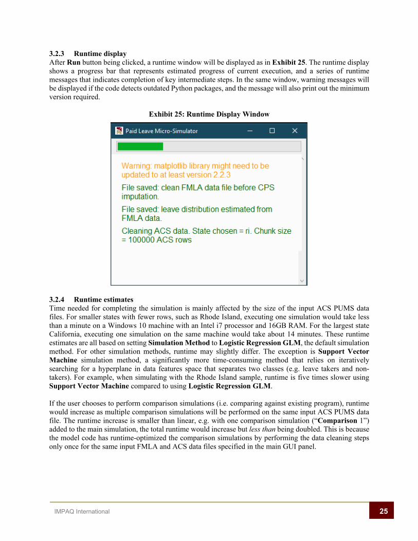
3.2.3 Runtime display After Run button being clicked, a runtime window will be displayed as in Exhibit 25. The runtime display shows a progress bar that represents estimated progress of current execution, and a series of runtime messages that indicates completion of key intermediate steps. In the same window, warning messages will be displayed if the code detects outdated Python packages, and the message will also print out the minimum version required.

Exhibit 25: Runtime Display Window

3.2.4 Runtime estimates Time needed for completing the simulation is mainly affected by the size of the input ACS PUMS data files. For smaller states with fewer rows, such as Rhode Island, executing one simulation would take less than a minute on a Windows 10 machine with an Intel i7 processor and 16GB RAM. For the largest state California, executing one simulation on the same machine would take about 14 minutes. These runtime estimates are all based on setting Simulation Method to Logistic Regression GLM, the default simulation method. For other simulation methods, runtime may slightly differ. The exception is Support Vector Machine simulation method, a significantly more time-consuming method that relies on iteratively searching for a hyperplane in data features space that separates two classes (e.g. leave takers and non-takers). For example, when simulating with the Rhode Island sample, runtime is five times slower using Support Vector Machine compared to using Logistic Regression GLM.

If the user chooses to perform comparison simulations (i.e. comparing against existing program), runtime would increase as multiple comparison simulations will be performed on the same input ACS PUMS data file. The runtime increase is smaller than linear, e.g. with one comparison simulation (“Comparison 1”) added to the main simulation, the total runtime would increase but less than being doubled. This is because the model code has runtime-optimized the comparison simulations by performing the data cleaning steps only once for the same input FMLA and ACS data files specified in the main GUI panel.


CHAPTER 4. INTERPRETING SIMULATION RESULTS 4.1 Simulation output Upon completion of simulation, a separate Results Window will be displayed, with numerical and graphical results grouped in a set of tabs. As illustrated in exhibits below, a Save Figure button is available for each graph, allowing users to save the graph in .PNG format by navigating to a desired local directory.

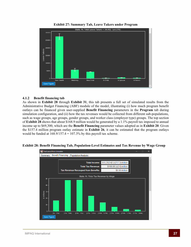
4.1.1 Summary tab As shown in Exhibit 26 and Exhibit 27, this tab presents two graphs. The first graph plots the simulated program benefit costs, and second plots the simulated number of leave takers participating the program. In each graph, the estimates are displayed for the six leave reasons. Total estimates of across the six leave reasons are respectively displayed in the plot titles. For the bars in each graph, the white interval represents the 95% confidence interval of the estimate derived from the 80 ACS PUMS replication weights.15 Users should note that the while the total benefit cost is the sum of benefit cost across leave types, the Total Leave Takers number represents total number of leave takers under program, among whom some may take leaves due to multiple reasons. Therefore, the Total Leave Takers number in the second graph is not necessarily equal to the sum of the number of leave takers across the six leave reasons – it is generally smaller than that sum due to the presence of multiple-reason leave takers.

Exhibit 26: Summary Tab, Program Benefit Costs

15 See https://usa.ipums.org/usa/repwt.shtml for details on Census methodology to compute standard errors using the replication weights.

https://usa.ipums.org/usa/repwt.shtml


Exhibit 27: Summary Tab, Leave Takers under Program

4.1.2 Benefit financing tab As shown in Exhibit 28 through Exhibit 31, this tab presents a full set of simulated results from the Administrative Budget Financing (ABF) module of the model, illustrating (i) how much program benefit outlays can be financed given user-supplied Benefit Financing parameters in the Program tab during simulation configuration, and (ii) how the tax revenues would be collected from different sub-populations, such as wage groups, age groups, gender groups, and worker class (employer type) groups. The top section of Exhibit 28 shows that about $168.9 million would be generated by a 1.1% payroll tax imposed to annual income up to $69,300, which are the Benefit Financing parameter values adopted as in Exhibit 20. Given the $157.4 million program outlay estimate in Exhibit 26, it can be estimated that the program outlays would be funded at 168.9/157.4 = 107.3% by this payroll tax scheme.

Exhibit 28: Benefit Financing Tab, Population-Level Estimates and Tax Revenue by Wage Group


Exhibit 29: Benefit Financing Tab, Tax Revenue by Gender

Exhibit 30: Benefit Financing Tab, Tax Revenue by Age Group

Exhibit 31: Benefit Financing Tab, Tax Revenue Class of Worker

Note: There is only one bar “Private” displayed since the model is configured as only allowing workers employed by private employers. More bars (such as one representing State government workers) will be displayed in this graph based on user choice of more eligible employer types.

At the bottom of the Benefit Financing tab, as shown in Exhibit 31, there is an ABF Parameters button. Clicking this button will enable an input box where user can update the Benefit Financing parameters to replace those previously specified under the Program tab during simulation configuration. The input box for updating Benefit Financing parameters are illustrated in Exhibit 32.


Exhibit 32: Updating Benefit Financing Parameters

Since benefit financing results are independent of simulations of leave taking and program outlay benefits, re-computing the benefit financing results can be done separately after the simulation using alternative payroll tax schemes. Users can specify Benefit Financing parameters and click the Run ABF button to update the results and charts in the Benefit Financing results tab. Runtime for this updating process is typically less than one minute for small states such as Rhode Island, and up to two to three minutes for larger states such as California. Users can use the Hide button to hide this input box if it is no longer needed.

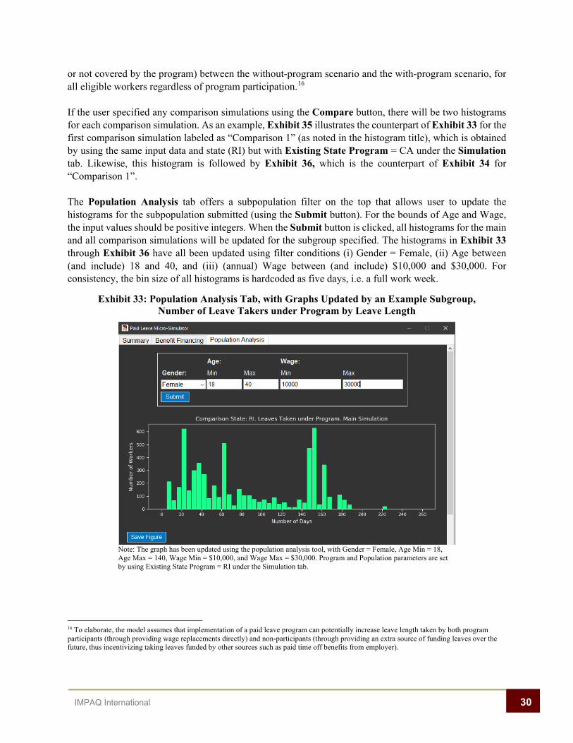
4.1.3 Population analysis tab As shown in Exhibit 33 and Exhibit 34, this tab presents two histograms of estimated worker counts for the main simulation (as noted in the title of each histogram).

The first histogram (Exhibit 33) shows the estimated number of workers in the state of interest (in this example, Rhode Island) by leave length (in number of days) taken under the program. This distribution provides information on the program’s direct benefit to program participants by focusing on the leave length covered by the program.

The second histogram (Exhibit 34) shows the estimated number of workers regardless of program participation by increase in leave length (in number days). This distribution provides information on the program’s indirect benefit to program participants by focusing on increase in leave length (either covered


or not covered by the program) between the without-program scenario and the with-program scenario, for all eligible workers regardless of program participation.16

If the user specified any comparison simulations using the Compare button, there will be two histograms for each comparison simulation. As an example, Exhibit 35 illustrates the counterpart of Exhibit 33 for the first comparison simulation labeled as “Comparison 1” (as noted in the histogram title), which is obtained by using the same input data and state (RI) but with Existing State Program = CA under the Simulation tab. Likewise, this histogram is followed by Exhibit 36, which is the counterpart of Exhibit 34 for “Comparison 1”.

The Population Analysis tab offers a subpopulation filter on the top that allows user to update the histograms for the subpopulation submitted (using the Submit button). For the bounds of Age and Wage, the input values should be positive integers. When the Submit button is clicked, all histograms for the main and all comparison simulations will be updated for the subgroup specified. The histograms in Exhibit 33 through Exhibit 36 have all been updated using filter conditions (i) Gender = Female, (ii) Age between (and include) 18 and 40, and (iii) (annual) Wage between (and include) $10,000 and $30,000. For consistency, the bin size of all histograms is hardcoded as five days, i.e. a full work week.

Exhibit 33: Population Analysis Tab, with Graphs Updated by an Example Subgroup, Number of Leave Takers under Program by Leave Length

Note: The graph has been updated using the population analysis tool, with Gender = Female, Age Min = 18, Age Max = 140, Wage Min = $10,000, and Wage Max = $30,000. Program and Population parameters are set by using Existing State Program = RI under the Simulation tab.

16 To elaborate, the model assumes that implementation of a paid leave program can potentially increase leave length taken by both program participants (through providing wage replacements directly) and non-participants (through providing an extra source of funding leaves over the future, thus incentivizing taking leaves funded by other sources such as paid time off benefits from employer).


Exhibit 34: Population Analysis Tab, Number of Leave Takers Regardless of Program Participation by Additional Leave Length due to Program Implementation

Note: The graph has been updated using the population analysis tool, with Gender = Female, Age Min = 18, Age Max = 140, Wage Min = $10,000, and Wage Max = $30,000. Program and Population parameters are set by using Existing State Program = RI under the Simulation tab.

Exhibit 35: Population Analysis Tab, Number of Leave Takers under Program by Leave Length,

Comparison Simulation

Note: The graph has been updated using the population analysis tool, with Gender = Female, Age Min = 18, Age Max = 140, Wage Min = $10,000, and Wage Max = $30,000. Program and Population parameters are set by using Existing State Program = RI under the Simulation tab. Program and Population parameters are set by using Existing State Program = CA under the Simulation tab.

Exhibit 36: Population Analysis Tab, Number of Leave Takers Regardless of Program Participation by Additional Leave Length due to Program Implementation,

Comparison Simulation


Note: The graph has been updated using the population analysis tool, with Gender = Female, Age Min = 18, Age Max = 140, Wage Min = $10,000, and Wage Max = $30,000. Program and Population parameters are set by using Existing State Program = CA under the Simulation tab.

4.2 Output folder Besides the results and graphs shown in the Results window, the Worker PLUS model also saves a set of individual-level data files and meta-data files in the output folder for each simulation, should users have more customized analytical needs. Upon completion of model running, an output folder will be created for each simulation (i.e. separately for the main simulation and for each comparison simulation) in the Output directory specified by the user in the main GUI panel. Each output folder is named in the format output_[yyyymmdd]_[hhmmss]_[header] where [yyyymmdd] and [hhmmss] respectively denote the date stamp and time stamp when the Run button is clicked for model execution, and [header] is a unique identifier for the main or comparison simulation. An example output folder name is output_20201029_195242_main simulation. The set of output data files in an output folder is illustrated in Exhibit 37. They include: • abf_acs_sim_[st]_[datestamp]_[timestamp].csv – This is a data set containing all eligible ACS

PUMS sample workers identified from the state [st]. In Exhibit 37, the state is Rhode Island; hence, the [st] part is “ri” in the file name. This file contains individual-level variables related to benefit financing, such as taxable wage income, payroll tax revenue, etc.

• abf_summary.csv – This is a population level data set providing population-level estimates from the ABF module. The numbers in this file are generated upon completion of simulation and will be updated as the user re-calculate the ABF estimates using the ABF Parameters button in the Benefit Financing tab. The date stamp and time stamp are not included in the file name as this file can be updated by re-calculation at a different time than the original simulation.

• acs_sim_[st]_[datestamp]_[timestamp].csv – This is a master post-simulation ACS PUMS data file for state [st]. This data file contains all eligible ACS workers in the state, with new columns generated from the simulation. These new columns include simulated leave taking status for different leave reasons, simulated proportion of pay during leave from employer, simulated leave length for different leave reasons, etc.

• prog_data_[datestamp]_[timestamp].csv – This is a meta-data file that stores the parameters used to configure the simulation, such as state and year chosen, simulation method, random seed, program eligibility rules, program take-up rates, program benefit payout schemes, benefit financing parameters, etc. The file allows user to keep track of all parameters used by the model for simulation.

• program_cost_[st]_[datestamp]_[timestamp].csv – This is a program cost summary file. The file summarizes program benefit costs across all six leave types and the total benefit cost. The file also provides the 95% confidence interval bounds for each simulated cost estimate.

• program_progtaker_[st]_[datestamp]_[timestamp].csv – This is a program participant summary file. The file summarizes program participant counts across all six leave types and the count of program participant due to any leave reason. The file also provides the 95% confidence interval bounds for each simulated cost estimate.

s


Exhibit 37: Files in the Output Directory


APPENDIX

Python Package Installation and Update via a Virtual Environment

The following guide applies only to users who choose the Model Execution Option 2 i.e. running the model using the source code in the microsim-dev folder. The guide does not apply to users who choose the Model Execution Option 1 (running the model using the Windows executable), as the required Python packages have been compiled into the executable.

For advanced Python users who choose the Model Execution Option 2 and do not wish to or cannot make changes to their current Python environment, the packages can be installed to a virtual environment in following steps:

1. Open the Windows Command Prompt or PowerShell. 2. Navigate to the microsim-dev directory. 3. Type the following commands, hitting enter after each command.

• python -m venv microsim-env • microsim-env\Scripts\activate.bat (from Command Prompt) or

microsim-env\Scripts\activate.ps1 (from PowerShell) • pip install –r requirements.txt

For the greatest simplicity, we recommend installing Anaconda, which can greatly facilitate Python package installation for Windows users. The Worker PLUS model will work with the Anaconda 5.3.0 or later distribution. Users with older releases can update their packages by running the command conda update --all. The only package not included in Anaconda distributions is mord, which can be installed using the command conda install –c mord using the Anaconda Prompt. Alternatively, users can also Windows Command Prompt or PowerShell and execute the command pip install mord. After completing the above installation steps, users should either proceed to Section 2.3.2 to further install the required R packages for using the R simulation engine, or directly proceed to Section 2.4 to open the model GUI for using the Python simulation engine.

https://www.anaconda.com/

Documents

Worker Paid Leave Usage Simulation Model User Manual