Embed Size (px)
Citation preview

INTERPLAN INTEgrated opeRation PLAnning tool towards
the Pan-European Network
Work Package 5
Operation planning and semi-dynamic simulation
Deliverable D5.2
Operation planning and semi-dynamic simulation of grid equivalents
Grant Agreement No: 773708
Funding Instrument: Research and Innovation Action (RIA)
Funded under: H2020 LCE-05-2017: Tools and technologies for coordination and integration of the European energy system
Starting date of project: 01.11.2017
Project Duration: 36 months
Contractual delivery date: 31.10.2019
Actual delivery date: 14.11.2019
Lead beneficiary: 1 ENEA Agenzia nazionale per le nuove tecnologie, l'energia e lo sviluppo economico sostenibile (ENEA)
Deliverable Type: Report (R)
Dissemination level: Public (PU)
Revision / Status: RELEASED
This project has received funding from the European Union’s Horizon 2020 Research and Innovation Programme under
Grant Agreement No. 773708

GA No: 773708
Deliverable: D5.2 Revision / Status: RELEASED 2 of 119
Document Information Document Version: 14
Revision / Status: RELEASED All Authors/Partners Marialaura Di Somma / ENEA Roberto Ciavarella / ENEA Giorgio Graditi / ENEA Maria Valenti / ENEA Helfried Brunner / AIT Mihai Calin / AIT Adolfo Anta / AIT Sawsan Henein / AIT Sohail Khan / AIT Ata Khavari / DERlab Christina Papadimitriou / FOSS Melios Hadjikypris / FOSS Venizelos Efthymiou / FOSS Jan Ringelstein / IEE Saber Talari/ DERlab, IEE Anna Wakszynska / IEn Michal Kosmecki / IEn Michal Bajor / IEn Distribution List INTERPLAN consortium Keywords: Integrated operation planning tool, base showcase, TSO, DSO,
TSO/DSO interaction, system operator, network operation planning, planning criteria, Python-based toolbox, key performance indicator, grid model, grid equivalent, flexibility resources, renewable energy sources, storage, demand response, optimization, distributed generation, control functions, frequency stability, voltage stability, system congestion, synchronous generator, inertia, tertiary control, active power control, reactive power control, test case, dynamic simulation, semi-dynamic simulation, PowerFactory, simulation results
Document History
Revision Content / Changes Resp. Partner Date
1 Structure created ENEA 13.09.2019
2 INTERPLAN tool description added ENEA 19.09.2019
3 Some comments and revisions added for the INTERPLAN tool
description FOSS, IEn 25.09.2019
4 Input added to address comments for the INTERPLAN tool ENEA, IEn, IEE, AIT 10.10.2019
5 Executive summary, Sections 1, 2 and 3 added ENEA 21.10.2019
6 Base showcases properties added for BSC 2, 3, 4, 5 ENEA, AIT, FOSS,
IEE, IEn 22.10.2019
7 Test cases properties added for BSC 2, 3, 4, 5 ENEA, AIT, IEE, IEn 24.10.2019
8 Test cases results added for BSC 2, 3, 5 ENEA, AIT, IEE, IEn 24.10.2019
9 Revisions added for BSC 2,3,4 and 5 ENEA 25.10.2019

GA No: 773708
Deliverable: D5.2 Revision / Status: RELEASED 3 of 119
10 BSC 1 and results for BSC4 added FOSS, DERlab 28.10.2019
11 Conclusions added ENEA 28.10.2019
12 Document finalized for review ENEA 29.10.2019
13 Reviewers’ comments addressed ENEA, IEE, FOSS,
DERlab, IEn 13.11.2019
14 Deliverable finalized ENEA 14.11.2019
Document Approval
Final Approval Name Resp. Partner Date
Review Task Level Marialaura Di Somma
Ata Khavari
ENEA
DERlab
29.10.2019
07.11.2019
Review WP Level Jan Ringlestein
(review of BSCs simulation results) IEE 04.11.2019
Review Management Level Helfried Brunner
Giorgio Graditi
AIT
ENEA
05.11.2019
14.11.2019
Disclaimer This document contains material, which is copyrighted by certain INTERPLAN consortium parties
and may not be reproduced or copied without permission. The information contained in this
document is the proprietary confidential information of certain INTERPLAN consortium parties and
may not be disclosed except in accordance with the consortium agreement.
The commercial use of any information in this document may require a licence from the proprietor of
that information.
Neither the INTERPLAN consortium as a whole, nor any single party within the INTERPLAN
consortium warrant that the information contained in this document is capable of use, nor that the
use of such information is free from risk. Neither the INTERPLAN consortium as a whole, nor any
single party within the INTERPLAN consortium accepts any liability for loss or damage suffered by
any person using the information.
This document does not represent the opinion of the European Community, and the European
Community is not responsible for any use that might be made of its content.
Copyright Notice © The INTERPLAN Consortium, 2017 - 2020

GA No: 773708
Deliverable: D5.2 Revision / Status: RELEASED 4 of 119
Table of contents
Abbreviations ....................................................................................................................................... 5
Executive Summary ............................................................................................................................. 6
1. Introduction ................................................................................................................................... 8
1.1 Purpose and scope of the Document ................................................................................... 8 1.2 Structure of the Document .................................................................................................... 8
2. INTERPLAN project ...................................................................................................................... 9
3. Methodology ............................................................................................................................... 11
3.1 INTERPLAN Integrated Operation Planning tool development ......................................... 11 3.2 Base showcases simulation ................................................................................................ 12
4. INTERPLAN Integrated Operation Planning Tool for the Pan-European Network ................... 14
4.1 INTERPLAN tool overview .................................................................................................. 14 4.2 Stage 1 - Simulation functionalities, KPIs and scenario selection ..................................... 16 4.3 Stage 2 - Grid model selection/preparation ........................................................................ 31 4.4 Stage 3 – Simulation & Evaluation...................................................................................... 38
5. Simulation of grid equivalents for base showcases ................................................................... 40
5.1 Low inertia systems - BSC1 ................................................................................................ 41 5.2 Effective DER operation planning through active and reactive power control - BSC2 ...... 60 5.3 TSO-DSO power flow optimization - BSC3 ........................................................................ 70 5.4 Active and reactive power flow optimization at transmission and distribution networks - BSC4 ............................................................................................................................................. 80 5.5 Optimal energy interruption management - BSC5 ............................................................. 92
6. Summary and outlook ............................................................................................................... 112
7. References................................................................................................................................ 115
8. Annex ........................................................................................................................................ 116
8.1 List of Figures .................................................................................................................... 116 8.2 List of Tables ..................................................................................................................... 116 8.3 Glossary of terms and definitions...................................................................................... 116

GA No: 773708
Deliverable: D5.2 Revision / Status: RELEASED 5 of 119
Abbreviations
AENS Average energy not supplied
BESS Battery energy storage system
BSC Base showcase
BUC Base use case
cdf Cumulative distribution function
DER Distributed energy resources
DG Distributed generation
DR Demand response
RES Renewable energy sources
DRES Distributed renewable energy resources
DSL DIgSILENT Simulation Language
DSO Distribution system operator
EHV Extra high voltage
ENS Energy not supplied
ENTSO-E European Network of Transmission System Operators for Electricity
EU European Union
EV Electric vehicle
fFRC Fast frequency restoration control
HV High voltage
IEAR Interrupted energy assessment rate
IEX Information exchanged
INTERPLAN Integrated operation planning tool for the pan-European network
KPI Key performance indicator
LV Low voltage
LF Load Flow
MV Medium voltage
OPF Optimal Power Flow
PV Photovoltaic
RES Renewable energy sources
RMS Stability Analysis Functions
RoCoF Rate of change of frequency
SAIDI System average interruption duration index
SAIFI System average interruption frequency index
SC Showcase
SI System inertia
TSO Transmission system operator
UC Use case
UFLS Under-frequency load shedding
WTG Wind turbine generator

GA No: 773708
Deliverable: D5.2 Revision / Status: RELEASED 6 of 119
Executive Summary
The document provides the detailed description of the INTERPLAN Integrated Network Operation
Planning tool and presents the results of the dynamic and semi-dynamic simulations for the five
INTERPLAN base showcases [1].
The INTERPLAN tool is defined as a methodology consisting of a set of tools (grid equivalents,
control functions) for the operation planning of the Pan-European network by addressing a significant
number of system operation planning challenges of the current and the future 2030+ EU power grid,
from the perspective of the transmission system, the distribution system, and with a particular focus
on the transmission-distribution interface. In this sense, the main goal of the tool is to achieve the
operation planning of an integrated grid from the perspective of a transmission system operator
(TSO) or a distribution system operator (DSO) through handling efficiently and effectively intermittent
renewable energy resources (RES) as well as the emerging technologies such as storage, demand
response and electric vehicles. In fact, the tool supports utilizing flexibility potential coming from
RES, Demand Side Management, storage and electric mobility for system services in all network
control levels.
The INTERPLAN tool consists of three main stages (1. Simulation functionalities, Key Performance
Indicators (KPIs) and scenario selection, 2. Grid model selection/preparation, 3. Simulation &
Evaluation). First of all, the user identified as a TSO or a DSO selects the planning criteria that he
wants to consider for the network operation planning. This selection is based on the list of planning
criteria identified by INTERPLAN Consortium.
Under the stage 1, the user selects the simulation functionality, the KPIs and the operating future
scenario among the four INTERPLAN scenarios [2] with the related target year. The stage 2 of
INTERPLAN tool is dedicated to the grid model selection and preparation. Under this stage, the user
selects the grid model for the simulation phase in the next stage, and it is then adapted to the
INTERPLAN scenario selected under the previous stage. If a grid equivalent model is required for
the simulation phase, the system operator can select it from the grid equivalents library consisting of
a list of pre-defined grid equivalents, or can preferably generate a grid equivalent model through the
grid equivalent generation procedure made available by the INTERPLAN tool. When the grid model
is decided, it is then adapted to the scenario selected under stage 1 through the scenario adaptation
procedure.
Finally, the stage 3 of INTERPLAN tool is dedicated to the simulation and evaluation phase. Under
this stage, the user performs the simulation by using one of the INTERPLAN control solutions
(INTERPLAN control functions embedded within the use cases or the showcases) according to the
operation challenge to be investigated and the choices done in the previous stages. The evaluation
phase follows the simulation one. In detail, here, the user makes an evaluation through the KPIs
found in simulation phase. If the user is satisfied with the KPI(s) found, the evaluation is complete
and the process stops. Otherwise, the user can decide to investigate further INTERPLAN solutions
addressing the same operation challenge under the same planning criteria. In this latter case, the
process re-starts from stage 1.
As for the second item addressed in this deliverable, it refers to the simulation of basic grid
equivalents [3] for the five INTERPLAN base showcases [1].
A base showcase is defined as a combination of sub base use case(s) with no planning criteria and
no controllers for emerging technologies, such as RES, distributed generation (DG), demand
response (DR) or storage technologies. For each of the five showcase defined in INTERPLAN, there

GA No: 773708
Deliverable: D5.2 Revision / Status: RELEASED 7 of 119
is a relevant base showcase with the same grid model, scenario, KPIs, simulation environment,
simulation type and time-series data. The simulations of base showcases actually allow to evaluate
effectiveness, reliability and robustness of the control functions proposed in the associated
showcases, which will be developed and implemented later in the project.

GA No: 773708
Deliverable: D5.2 Revision / Status: RELEASED 8 of 119
1. Introduction 1.1 Purpose and scope of the Document
The document presents the developed Integrated Operation Planning Tool for the Pan-European
Network and the simulations of basic grid equivalents for base showcases.
The main goals of the deliverable are described in the following:
• provide an overview of the INTERPLAN tool, with the main concepts and functionalities;
• present the main strengthen points of the tool for the perspective of the tool’s users (TSOs
and DSOs) for the operation planning of the Pan-European network;
• detail the main steps that the user has to perform in the three composing stages (simulation
functionalities, KPIs and scenario selection, grid model selection/preparation, simulation &
evaluation);
• define the main contents of the INTERPLAN user manual, which represents a guide for the
user, consisting of all the possible selections enabled to the user in the various steps;
• identify the potential developments of the INTERPLAN tool for further research and
advancement needed to make the tool usable in the real practice;
• establish the properties for INTERPLAN base showcases needed for their implementation;
• establish the properties of test cases needed to perform the simulations for the base
showcases;
• present the results of these simulations, by evaluating the KPIs with the aim to create a
foundation for comparison with INTERPLAN showcases and their embedded control
functions that will be developed later in the project. In the reporting of the results, the main
operation criticalities found in simulations as well as the possible solutions to apply through
control functions are also presented.
1.2 Structure of the Document
The deliverable consists of seven chapters. The purpose and scope of the deliverable are described
in the first chapter. The second chapter briefly introduces the INTERPLAN project. In the third
chapter, the methodology used to attain the results presented in this deliverable is presented.
The fourth chapter presents the INTERPLAN tool overview and the detailed description of the three
stages composing it. The simulations of basic grid equivalents for the five base showcases are
addressed in the sixth chapter. The seventh chapter is a summary of the report and an outlook for
the future activities, whereas in the Annex 1, the glossary of the terms and definitions used in the
INTERPLAN project can be found.

GA No: 773708
Deliverable: D5.2 Revision / Status: RELEASED 9 of 119
2. INTERPLAN project The European Union (EU) energy security policy faces significant challenges as we move towards
a pan-European network based on the wide diversity of energy systems among EU members. In
such a context, novel solutions are needed to support the future operation, resilience and reliability
of the EU electricity system in order to increase the security of supply and also accounting for the
increasing contribution of renewable energy sources (RES). The goal of the INTERPLAN project is
to provide an INTEgrated opeRation PLAnning tool towards the pan-European Network, with a focus
on the TSO-DSO interfaces to support the EU in reaching the expected low-carbon targets, while
maintaining the network security and reliability.
INTERPLAN project looks at the potential operation challenges which TSOs and DSOs are called to
address in the 2030+ power system. In fact, the ongoing deployment of the pan–European network
strongly depends on different potential scenarios related to the RES share in generation and installed
capacity, as well as penetration of emerging technologies, such as storage and Demand Response
(DR). Although these factors represent the preferential patterns to meet the EU decarbonized energy
targets for 2030 and 2050, they bring new challenges for the energy system, which will outline the
key operational needs of the European grid operators in the near future.
In such a context, TSOs will need to evolve progressively from a “business as usual approach” to a
proactive approach in order to avoid a bottleneck effect in the future European grid, and this could
be addressed through a proper system operation planning. As for the distribution networks, they
have been traditionally designed and treated to transport electrical energy in one direction, i.e., from
the generation units connected to the transmission system to the end-users. However, with the
growing share of non-dispatchable distributed generation, customers are increasingly generating
electricity themselves, and, by becoming “prosumers”, they are shifting from the end point to the
centre of the power system. As a result, DSOs will need to actively manage and operate a smarter
grid through appropriate system control logics, by utilizing the flexibility potential in the grid, with the
aim to optimize the distribution network performance. Furthermore, an additional critical issue is the
interface between transmission and distribution systems, which is expected to evolve in the near
future through a mutual cooperation between TSOs and DSOs, with the aim to address operational
challenges as congestion of transmission and distribution lines and at the interface among them,
voltage support between TSOs and DSOs, and power balancing concerns. The increasing
complexity of the grids requires control and operation planning tools even more advanced and
homogenous among European countries.
With these premises, the INTERPLAN idea was born. In such a framework, the projects aims to
develop control system logics which suit the complexity of the integrated grid, while managing all
relevant flexibility resources as “local active elements” in the best manner. Moreover, by looking at
the 2030+ power system, the project also addresses policy and regulation aspects aiming to identify
a set of possible amendments to the existing grid codes, reflecting the developments achieved in
INTERPLAN through its tool, use cases and showcases. The aim of this analysis is to break down
the current barriers to the integration of emerging technologies and to foster TSO-DSO cooperation
in managing grid operation challenges.
In detail, a methodology for a proper representation of a “clustered” model of the pan -European
network is provided, with the aim to generate grid equivalents as a growing library able to cover a
number of relevant system connectivity possibilities occurring in the real grid, by addressing a
number of operation planning issues at all network levels (transmission, distribution and TSO-DSO

GA No: 773708
Deliverable: D5.2 Revision / Status: RELEASED 10 of 119
interfaces). In this perspective, the chosen top-down approach leads to an “integrated” tool, both in
terms of voltage levels, moving from high voltage level down to low voltage level up to end user, as
well as in terms of developing a bridge between static, long-term planning and operational issues
considerations, by introducing proper control functions in the operation planning phase. Therefore,
in the project, novel control strategies and operation planning approaches are investigated in order
to ensure the security of supply and resilience of the interconnected EU electricity power networks,
based on a close cooperation between TSOs and DSOs, thereby responding to the crucial needs of
the ongoing pan-European network and its operators.
Figure 1: INTERPLAN concept

GA No: 773708
Deliverable: D5.2 Revision / Status: RELEASED 11 of 119
3. Methodology
3.1 INTERPLAN Integrated Operation Planning tool development
The INTERPLAN integrated network operation planning tool has been developed through the
following phases performed by the entire consortium.
First of all, the main concepts and the functionalities of the tool have been developed, by defining
the three main stages composing it and the related steps to be performed by the user:
• Stage 1: Simulation functionalities, KPIs and scenario selection;
• Stage 2: Grid model selection/preparation;
• Stage 3: Simulation & Evaluation.
The work started with defining the stage 1 of the tool, by extrapolating the main functionalities and
requirements of the INTERPLAN use cases and showcases documented in deliverables D3.2 [2]
and D5.1 [1], respectively. In detail, to establish the possible selections enabled to the user under
this stage, the individual planning criteria vs. applicable INTERPLAN use cases, the groups of the
planning criteria vs. the applicable INTERPLAN showcases as well as the sub-groups of planning
criteria vs. applicable INTERPLAN showcases have been first identified. Then, for each possible
combination i.e., single planning criterion/applicable use case, groups of planning criteria/applicable
showcases and sub-groups of planning criteria/applicable showcases, the selections of simulation
functionalities, KPIs and future scenarios enabled to the user have been identified.
As for stage 2 related to the grid model selection/preparation, the work to develop this stage has
been performed with a strong interaction with INTERPLAN approach for generating grid equivalents
for the different use cases and showcases. In detail, the grid equivalenting information related to
INTERPLAN use cases and showcases, which represent the requirements for grid equivalenting for
the use cases and showcases have been defined, as also documented in the public deliverable D4.2
[3]. These information mainly refer to:
• identify the grid(s) investigated for control;
• identify if a grid equivalent is required or not, by also understanding the feasibility to use a
grid equivalent model instead of the full model;
• identify the observable variables and parameters in the grid equivalent model
• identify the controllable variables and parameters in the grid equivalent model
• identify the requirements for the grid model
• identify the type of grid equivalent to apply.
As for the stage 3, the INTERPLAN solutions, which represent the control functions embedded in
the INTERPLAN use cases and showcases, have been identified.
In general, the INTERPLAN tool and its stages have been developed by taking into account the
following goals:
• Make the tool as responsive as possible to meet the critical needs of grid operators in
addressing a wide range of operation challenges covering all network levels and for
increasing TSO-DSO cooperation for operation planning purposes.
• Make the tool flexible enough to be adapted to the current and future grid scenarios.
• Make the tool flexible enough in the application of grid equivalents when they are needed for

GA No: 773708
Deliverable: D5.2 Revision / Status: RELEASED 12 of 119
studying specific operation challenges covering multiple voltage levels.
• Make the tool flexible enough in the integration of the various sub-tools and components
developed or to be developed in INTERPLAN (planning criteria, KPIs, scenarios, grid
equivalenting, use cases and showcases with the related control functions).
• Make the tool feasible for its application in real practice, by also identifying how the tool could
look like in the future.
To achieve these goals, the consortium has also counted on the feedbacks and opinions of relevant
external stakeholders. An example of this interaction is the INTERPLAN stakeholder workshop
“Innovative Network Operation Planning Tool for the TSO and DSO” organized as a parallel session
of the 2nd International Conference on Smart Energy Systems and Technologies (SEST 2019), held
in Porto on September 2019. A session of this workshop was in fact dedicated to the presentation of
the INTERPLAN tool to a broad audience and external panelists representative of European TSOs,
DSOs, academia and industry, who provided valuable feedback on the direction the developments
of the tool should take.
3.2 Base showcases simulation
Another important INTERPLAN activity regards the base showcases simulation. INTERPLAN base
showcase is defined as a combination of sub base use case(s) with no planning criteria and no
controllers for emerging technologies, such as RES, DG, DR or storage technologies. Base
showcases consist of base sub use cases, described for each use case in deliverable 3.2 [2], and
allow to analyze the operation challenges of the related use case(s). For each INTERPLAN
showcase (1. Low inertia systems; 2. Effective DER operation planning through active and reactive
power control; 3. TSO-DSO power flow optimization; 4. Active and reactive power flow optimization
at transmission and distribution networks; and 5. Optimal energy interruption management) [1], there
is a relevant base showcase with the same grid model, scenario, KPIs, simulation environment,
simulation type and time-series data. The simulation of base showcases is a key aspect to evaluate
effectiveness, reliability and robustness of the control functions proposed in the associated
showcases, which will be developed and implemented later in the project. This activity has been performed by the entire consortium and can be divided in the following phases:
• Establishment of base showcase properties (related description; sequence diagram, timing
diagram, sequence of actions, domain and scenario under investigation). In this phase, the
base showcases documented in deliverable D5.1 [2] have been further developed (and
revised in some cases) in order to allow their effective implementation in the simulation
environment.
• Establishment of test case properties (narrative of the test case, system under test, objects
under test, functions under test, KPIs under test, simulation environment, simulation type,
time-series data objects, output parameters, temporal resolution, suspension criteria /
stopping criteria). Moreover, in this phase, the scenario selected for each base showcase
has been adapted to the grid model used for the simulation, and the time-series data have
been defined accordingly.
• Test case reporting (KPIs evaluation, network operation criticalities found and possible
solutions identified to be implemented in the associated showcase). This phase allowed the
consortium to report the results found in the simulations, by also defining some potential
solutions to be considered for the future development of the control functions.
This activity has been carried out for all INTERPLAN base showcases and has seen the involvement

GA No: 773708
Deliverable: D5.2 Revision / Status: RELEASED 13 of 119
of all partners divided into working groups. The goal to perform simulations of base showcases is to
detect possible criticalities and identify possible solutions, by properly managing appropriate control
parameters, which will be the base to build up the control logics in the final project phase. In this
sense, a base showcase represents a reference case, with which the results attained by introducing
control functions in the grid operation planning, will be compared.
GA No: 773708
Deliverable: D5.2 Revision / Status: RELEASED 14 of 119
4. INTERPLAN Integrated Operation Planning Tool for the Pan-European Network
The INTERPLAN tool is defined as a methodology consisting of a set of tools (grid equivalents,
control functions) for the operation planning of the Pan-European network by addressing a significant
number of system operation planning challenges of the current and the future 2030+ EU power grid,
from the perspective of the transmission system, the distribution system, and with a particular focus
on the transmission-distribution interface. In this sense, the main goal of the tool is to achieve the
operation planning of an integrated grid from the perspective of a TSO or a DSO through handling
efficiently and effectively intermittent RES as well as the emerging technologies such as storage,
demand response and electric vehicles (EV). In fact, the tool supports utilizing flexibility potential
coming from RES, demand side management, storage and electric vehicles for system services in
all network control levels.
In the following, the overview of the tool will be discussed in Section 4.1, whereas the three stages
composing the tool will be described in detail in Sections 4.2, 4.3 and 4.4.
4.1 INTERPLAN tool overview
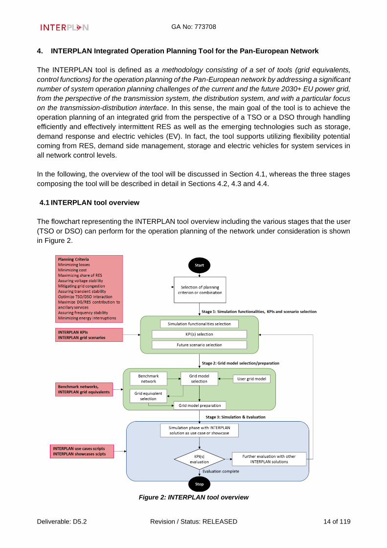
The flowchart representing the INTERPLAN tool overview including the various stages that the user
(TSO or DSO) can perform for the operation planning of the network under consideration is shown
in Figure 2.
Figure 2: INTERPLAN tool overview

GA No: 773708
Deliverable: D5.2 Revision / Status: RELEASED 15 of 119
As shown in the figure above, the user identified as a TSO or a DSO selects the planning criteria to
be considered for the network operation planning. This selection is based on the list of planning
criteria identified by INTERPLAN consortium as below:
1. Minimizing losses
2. Minimizing cost
3. Maximizing share of RES
4. Assuring voltage stability
5. Mitigating grid congestion
6. Assuring transient stability
7. Optimize TSO/DSO interaction
8. Maximize DG/RES contribution to ancillary services
9. Assuring frequency stability
10. Minimizing energy interruptions
After the planning criteria selection, the following three stages are performed by the user:
• Stage 1: Simulation functionalities, KPIs and scenario selection
• Stage 2: Grid model selection/preparation
• Stage 3: Simulation & Evaluation
Assuming that the user from the beginning has in mind the operation challenge to be investigated
through the tool, the various stages allow guiding the user’s choices towards the most suitable
INTERPLAN solution (use case- and showcase-related control functions) to apply. The various steps
composing the three stages have been structured to guide the user selecting the most proper
INTERPLAN solution in function of the operation challenge the user wants to investigate in a specific
network as part of the distribution system, the transmission system or the transmission-distribution
system. According to this approach, all the possible selections enabled will be known to the user in
advance through the INTERPLAN user manual.
Under the stage 1, the user selects the simulation functionality, the KPIs and the operating future
scenario.
The simulation functionality can be selected from the list of simulation functionalities used for the
INTERPLAN use cases and showcases. Similarly, the KPIs selection can be done from the list of
INTERPLAN KPIs and the operating scenario can be selected among the four INTERPLAN
scenarios. These types of choices can be done according to pre-defined schemes consisting of the
possible combinations enabled to the user that are use cases- and showcases-oriented.
The stage 2 of INTERPLAN tool is dedicated to the grid model selection and preparation. Under this
stage, the user selects the grid model for the simulation phase in the next stage, and it is then
adapted to the INTERPLAN scenario selected under the previous stage. In detail, under stage 2 the
user can select his own grid model and/or a benchmark grid model. Then, if a grid equivalent model
is required for the simulation phase – based on pre-defined requirements for grid equivalenting – the
user can select it from the grid equivalents library consisting of a list of pre-defined grid equivalents.
In case any of the grid equivalents present in the library is not suitable for the studies the user wants
to conduct, the user can generate a grid equivalent model through the grid equivalent generation
procedure made available by the INTERPLAN tool. When the grid model is decided, it is then
adapted to the scenario selected under stage 1 through the scenario adaptation procedure available
in the tool.

GA No: 773708
Deliverable: D5.2 Revision / Status: RELEASED 16 of 119
Finally, the stage 3 of INTERPLAN tool is dedicated to the simulation and evaluation phase. Under
this stage, the user performs the simulation either directly without selecting any of the INTERPLAN
solutions (use case- and showcase-related control functions) for creating an own reference case, or
by using one of the INTERPLAN solutions according to the operation challenge that the user wants
to investigate and the choices done in the previous stages. The evaluation phase follows the
simulation one. In detail, here, the user makes his evaluation through the KPIs found in simulation
phase. If the user is satisfied with the KPI(s) found, the evaluation is complete and the process stops.
Otherwise, the user can decide to investigate further INTERPLAN solutions addressing the same
operation challenge under the same planning criteria. In this latter case, the process re-starts from
stage 1.
The strengthen points of the tool developed are described below:
• It allows facing with the operation planning of the Pan-European network through an
integrated approach. In fact, by offering the possibility to investigate all network voltage levels
for operational planning purposes, the tool actually allows also integrating the actions made
by different stakeholders such as TSOs and DSOs, which are considered as the primary
users for the tool. In addition, this integrated approach allows building a bridge between
static, long-term planning and considering operational issues by introducing proper control
functions in the day-ahead operation planning phase.
• With the current network operation planning approaches, it is not possible to consider all
existing networks (including full models) in an integrated planning tool due to computational
limitations, lack of detailed models, etc. Through the intrinsic grid equivalenting methodology,
the tool allows simplifying certain parts of a grid while keeping the relevant characteristics.
This grid equivalenting methodology which is applicable to both transmission and distribution
levels results to be needed for TSO-DSO interactions, especially in the presence of flexibility
resources mainly connected at medium voltage (MV) and low voltage (LV) levels, which can
be used to address operational challenges occurring at all network levels.
• Through the control functions embedded within INTERPLAN use cases and showcases, the
tool allows addressing a number of operational challenges of the current and future 2030+
power networks from the perspective of both TSOs and DSOs. In detail, INTERPLAN use
cases address very specific operational challenges that grid operators may face with, in the
presence of high penetration of RES, storage, DR and EVs. On the other hand, INTERPLAN
showcases address a combination of operation challenges, thereby representing typical
cases that the grid operators may typically face with, for grid operation planning purposes.
From the practical point of view, in the future, the INTERPLAN toolset can be transformed into a
Python-based toolbox interfacing with PowerFactory (under the simulation phase in stage 3),
consisting of grid equivalents and control functions for use cases and showcases for addressing the
related operational challenges under the selected scenario and operation planning criteria.
The “proof-of-concept” of the INTERPLAN tool will be verified in upcoming tasks, through one of the
INTERPLAN use cases or showcases selected by the consortium also based on the consultation
with external relevant stakeholders.
4.2 Stage 1 - Simulation functionalities, KPIs and scenario selection
The flowchart representing the detailed steps that the user performs under stage 1 of the
INTERPLAN tool is shown in Figure 3.

GA No: 773708
Deliverable: D5.2 Revision / Status: RELEASED 17 of 119
Figure 3: Stage 1 of INTERPLAN tool
Before the stage 1, in selection of planning criteria, the user can select one single planning criterion
or a group/subgroup of planning criteria.
In case of selection of one single planning criterion, for each planning criterion, one or more use
cases with high relevance for that planning criterion can be suggested as possible solutions,
according to the table below.
Table 1: Individual planning criteria vs applicable INTERPLAN use cases
Planning criteria UC ID
1.Minimizing losses
UC1: Coordinated grid voltage/reactive power control
4. Assuring voltage stability
7. Optimize TSO/DSO interaction
8. Maximize DG / DRES contribution to ancillary
services
5. Mitigating grid congestion
UC2: Grid Congestion management 8. Maximize DG / DRES contribution to ancillary
services
1. Minimizing losses UC3: Frequency tertiary control based on optimal
power flow 2. Minimizing cost
3. Maximizing share of RES

GA No: 773708
Deliverable: D5.2 Revision / Status: RELEASED 18 of 119
7. Optimize TSO/DSO interaction
8. Maximize DG / DRES contribution to ancillary
services
6. Assuring transient stability
UC4: Fast Frequency Restoration Control 8.Maximize DG / DRES contribution to ancillary
services
9. Assuring frequency stability
1. Minimizing losses
UC5: Power balancing at DSO level
7. Optimize TSO/DSO interaction
8. Maximize DG / DRES contribution to ancillary
services
3. Maximizing share of RES
6. Assuring transient stability
UC6: Inertia management 8. Maximize DG / DRES contribution to ancillary
services
9. Assuring frequency stability
1. Minimizing losses
UC7: Energy interruption management 3. Maximizing share of RES
4. Assuring voltage stability
10. Minimizing energy interruptions
In case of selection of multiple planning criteria, for each group of planning criteria, the corresponding
showcase can be suggested according to the table below.
Table 2: Groups of planning criteria vs applicable INTERPLAN showcases
Group of planning criteria SC ID
6. Assuring transient stability
8.Maximize DG / DRES contribution to
ancillary services
9. Assuring frequency stability
SC1: Low inertia systems
1.Minimizing losses
3. Maximizing share of RES
4. Assuring voltage stability
5. Mitigating grid congestion
7. Optimize TSO/DSO interaction
8. Maximize DG / DRES contribution to
ancillary services
SC2: Effective DER operation planning through active and
reactive power control
1. Minimizing losses
2. Minimizing cost
3. Maximizing share of RES
7. Optimize TSO/DSO interaction
8. Maximize DG / DRES contribution to
ancillary services
SC3: TSO-DSO power flow optimization
1. Minimizing losses
2. Minimizing cost
3. Maximizing share of RES
7. Optimize TSO/DSO interaction
8. Maximize DG / DRES contribution to
ancillary services
SC4: Active and reactive power flow optimization at
transmission and distribution network

GA No: 773708
Deliverable: D5.2 Revision / Status: RELEASED 19 of 119
1. Minimizing losses
2. Minimizing cost
3. Maximizing share of RES
4. Assuring voltage stability
10. Minimizing energy interruptions
SC5: Optimal energy interruption management
In addition, the user can also select a sub-group of planning criteria and for each of these sub-
groups, one or more showcases can be suggested according to the table below.
Table 3: Sub-groups of planning criteria vs applicable INTERPLAN showcases
Sub-group of planning criteria SC ID
1. Minimizing losses
3. Maximizing share of RES
SC2: Effective DER operation planning through active and
reactive power control
SC3: TSO-DSO power flow optimization
SC4: Active and reactive power flow optimization at
transmission and distribution network
SC5: Optimal energy interruption management
1. Minimizing losses
2. Minimizing cost
3. Maximizing share of RES
SC3: TSO-DSO power flow optimization
SC4: Active and reactive power flow optimization at
transmission and distribution network
SC5: Optimal energy interruption management
3. Maximizing share of RES
7. Optimize TSO/DSO interaction
8. Maximize DG / DRES contribution to
ancillary services
SC2: Effective DER operation planning through active and
reactive power control
SC3: TSO-DSO power flow optimization
SC4: Active and reactive power flow optimization at
transmission and distribution network
7. Optimize TSO/DSO interaction
8. Maximize DG / DRES contribution to
ancillary services
SC2: Effective DER operation planning through active and
reactive power control
SC3: TSO-DSO power flow optimization
SC4: Active and reactive power flow optimization at
transmission and distribution network
3. Maximizing share of RES
4. Assuring voltage stability
SC2: Effective DER operation planning through active and
reactive power control
SC5: Optimal energy interruption management
After the selection of planning criteria, the stage 1 starts. In turn, it consists of three steps, as
specified below:
• Step 1.1: Selection of the simulation functionality. In this step, the user can select the
simulation functionalities among those available for simulating the INTERPLAN use cases
and showcases. The complete list is below:
o Optimal Power Flow (OPF);
o Basic Load Flow (LF);
o LF sensitivities;
o Stability Analysis Functions (RMS simulation);
o Optimization tool;
o Reliability assessment.
Note that also multiple simulation functionalities can be selected as specific packages according
to the requirements of INTERPLAN use cases and showcases as specified in Table 5 presented
later.

GA No: 773708
Deliverable: D5.2 Revision / Status: RELEASED 20 of 119
• Step 1.2: Selection of KPI(s). In this step, the user selects the KPI(s) addressing the planning
criteria previously chosen among the INTERPLAN KPIs, according to the table below.
Table 4: Key performance indicators vs planning criteria1
Key Performance Indicator ID Planning
criteria ID
1. Level of losses in transmission and distribution networks 1. Minimizing
losses 7. Power losses
4. Cost of service/energy interruption 2. Minimizing
cost 9. Interrupted Energy Assessment Rate
19. Generation costs
17. RES curtailment 3. Maximizing
share of RES 27. Share of RES
10. Voltage Quality: Voltage magnitude variations
4. Assuring
voltage
stability
12. Quadratic deviation from global reactive power production target
13. Mean quadratic deviations from voltage and reactive power targets at each connection
point between TSO and DSO grids
24. Reactive energy provided by RES and DG
2. Congestion detection
5. Mitigating
grid
congestion
6. Response time
6. Assuring
transient
stability
20. Frequency nadir/zenith
21. Rate of change of frequency
25. Indication of stability
26. Oscillation damping
11. Tap position changes per time
7. Optimize
TSO/DSO
interaction
12. Quadratic deviation from global reactive power production target
13. Mean quadratic deviations from voltage and reactive power targets at each connection
point between TSO and DSO grids
16. Transformer loading at TSO-DSO connection point
22. Quadratic deviation from global active power production target
23. Mean quadratic deviations from active power targets at each connection point between
TSO and DSO grids
14. Level of DG / DRES utilization for ancillary services
8. Maximize
DG/RES
contribution to
ancillary
services
5. Frequency restoration control effectivness
9. Assuring
frequency
stability
6. Response time
20. Frequency nadir/zenith
21. Rate of change of frequency
22. Quadratic deviation from global active power production target
23. Mean quadratic deviations from active power targets at each connection point between
TSO and DSO grids
25. Indication of stability
3. SAIDI (System Average Interruption Duration Index) 10.
Minimizing 18. SAIFI (System Average Interruption Frequency Index)
1 Details on the calculation method for these KPIs can be found in [2].
GA No: 773708
Deliverable: D5.2 Revision / Status: RELEASED 21 of 119
8. Energy not supplied energy
interruptions 9. Interrupted Energy Assessment Rate
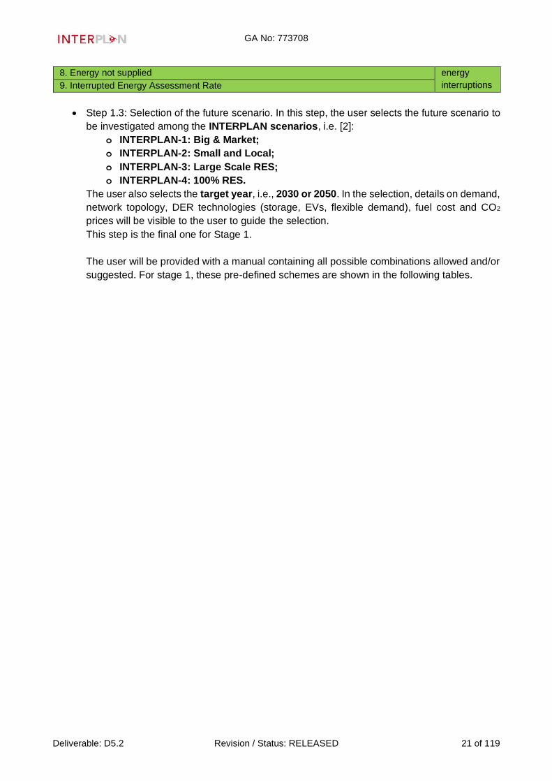
• Step 1.3: Selection of the future scenario. In this step, the user selects the future scenario to
be investigated among the INTERPLAN scenarios, i.e. [2]:
o INTERPLAN-1: Big & Market;
o INTERPLAN-2: Small and Local;
o INTERPLAN-3: Large Scale RES;
o INTERPLAN-4: 100% RES.
The user also selects the target year, i.e., 2030 or 2050. In the selection, details on demand,
network topology, DER technologies (storage, EVs, flexible demand), fuel cost and CO2
prices will be visible to the user to guide the selection.
This step is the final one for Stage 1.
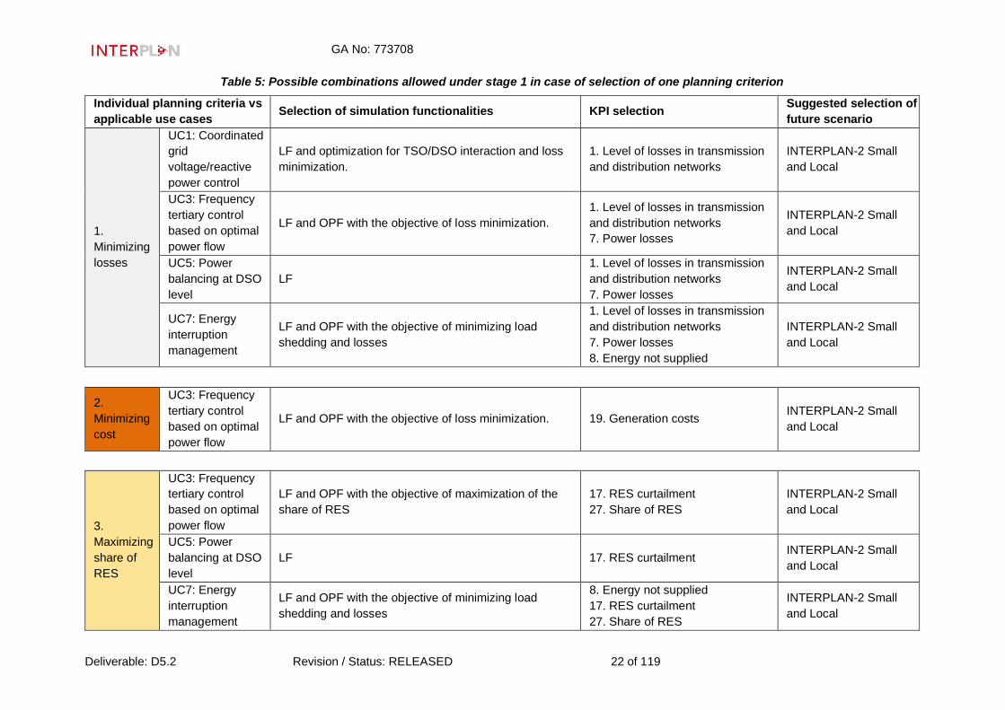
The user will be provided with a manual containing all possible combinations allowed and/or
suggested. For stage 1, these pre-defined schemes are shown in the following tables.
GA No: 773708
Deliverable: D5.2 Revision / Status: RELEASED 22 of 119
Table 5: Possible combinations allowed under stage 1 in case of selection of one planning criterion
Individual planning criteria vs
applicable use cases Selection of simulation functionalities KPI selection
Suggested selection of
future scenario
1.
Minimizing
losses
UC1: Coordinated
grid
voltage/reactive
power control
LF and optimization for TSO/DSO interaction and loss
minimization.
1. Level of losses in transmission
and distribution networks
INTERPLAN-2 Small
and Local
UC3: Frequency
tertiary control
based on optimal
power flow
LF and OPF with the objective of loss minimization.
1. Level of losses in transmission
and distribution networks
7. Power losses
INTERPLAN-2 Small
and Local
UC5: Power
balancing at DSO
level
LF
1. Level of losses in transmission
and distribution networks
7. Power losses
INTERPLAN-2 Small
and Local
UC7: Energy
interruption
management
LF and OPF with the objective of minimizing load
shedding and losses
1. Level of losses in transmission
and distribution networks
7. Power losses
8. Energy not supplied
INTERPLAN-2 Small
and Local
2.
Minimizing
cost
UC3: Frequency
tertiary control
based on optimal
power flow
LF and OPF with the objective of loss minimization. 19. Generation costs INTERPLAN-2 Small
and Local
3.
Maximizing
share of
RES
UC3: Frequency
tertiary control
based on optimal
power flow
LF and OPF with the objective of maximization of the
share of RES
17. RES curtailment
27. Share of RES
INTERPLAN-2 Small
and Local
UC5: Power
balancing at DSO
level
LF 17. RES curtailment INTERPLAN-2 Small
and Local
UC7: Energy
interruption
management
LF and OPF with the objective of minimizing load
shedding and losses
8. Energy not supplied
17. RES curtailment
27. Share of RES
INTERPLAN-2 Small
and Local

GA No: 773708
Deliverable: D5.2 Revision / Status: RELEASED 23 of 119
4. Assuring
voltage
stability
UC1: Coordinated
grid
voltage/reactive
power control
LF and optimization for TSO/DSO interaction and loss
minimization.
10. Voltage Quality: Voltage
magnitude variations
12. Quadratic deviation from global
reactive power production target
13. Mean quadratic deviations from
voltage and reactive power targets
at each connection point between
TSO and DSO grids
24. Reactive energy provided by
RES and DG
INTERPLAN-2 Small
and Local
UC7: Energy
interruption
management
LF and OPF with the objective of minimizing load
shedding and losses
10. Voltage Quality: Voltage
magnitude variations
13. Mean quadratic deviations from
voltage and reactive power targets
at each connection point between
TSO and DSO grids
INTERPLAN-2 Small
and Local
5. Mitigating
grid
congestion
UC2: Grid
Congestion
management
LF and LF Sensitivities 2. Congestion detection INTERPLAN-2 Small
and Local
6. Assuring
transient
stability
UC4: Fast
Frequency
Restoration
Control
RMS simulation, LF
5. Frequency restoration control
effectiveness
6. Response time
INTERPLAN-3: Large
Scale RES
UC6: Inertia
management RMS simulation, LF
20. Frequency nadir/zenith
21. Rate of change of frequency
25. Indication of stability
26. Oscillation damping
INTERPLAN-3: Large
Scale RES
7. Optimize
TSO/DSO
interaction
UC1: Coordinated
grid
voltage/reactive
power control
LF and optimization for TSO/DSO interaction and loss
minimization.
11. Tap position changes per time
12. Quadratic deviation from global
reactive power production target
INTERPLAN-2 Small
and Local

GA No: 773708
Deliverable: D5.2 Revision / Status: RELEASED 24 of 119
13. Mean quadratic deviations from
voltage and reactive power targets
at each connection point between
TSO and DSO grids
UC3: Frequency
tertiary control
based on optimal
power flow
LF and OPF at both operating levels
22. Quadratic deviation from global
active power production target
23. Mean quadratic deviations from
active power targets at each
connection point between TSO and
DSO grids
INTERPLAN-2 Small
and Local
UC5: Power
balancing at DSO
level
LF 16. Transformer loading at TSO-
DSO connection point
INTERPLAN-2 Small
and Local
8. Maximize
DG / DRES
contribution
to ancillary
services
UC1: Coordinated
grid
voltage/reactive
power control
LF and optimization for TSO/DSO interaction and loss
minimization.
14. Level of DG / DRES utilization
for ancillary services
INTERPLAN-2 Small
and Local
UC2: Grid
Congestion
management
LF and LF Sensitivities 14. Level of DG / DRES utilization
for ancillary services
INTERPLAN-2 Small
and Local
UC3: Frequency
tertiary control
based on optimal
power flow
LF and OPF with the objective of loss minimization 14. Level of DG / DRES utilization
for ancillary services
INTERPLAN-2 Small
and Local
UC4: Fast
Frequency
Restoration
Control
RMS simulation, LF 14. Level of DG / DRES utilization
for ancillary services
INTERPLAN-3: Large
Scale RES
UC5: Power
balancing at DSO
level
LF 14. Level of DG / DRES utilization
for ancillary services
INTERPLAN-2 Small
and Local
UC6: Inertia
management RMS simulation, LF
14. Level of DG / DRES utilization
for ancillary services
INTERPLAN-3: Large
Scale RES

GA No: 773708
Deliverable: D5.2 Revision / Status: RELEASED 25 of 119
UC7: Energy
interruption
management
LF and OPF with the objective of minimizing load
shedding and losses
2. Congestion detection
10. Voltage Quality: Voltage
magnitude variations
14. Level of DG / DRES utilization
for ancillary services
17. RES curtailment
INTERPLAN-2 Small
and Local
9. Assuring
frequency
stability
UC4: Fast
Frequency
Restoration
Control
RMS simulation, LF
5. Frequency restoration control
effectiveness
6. Response time
INTERPLAN-3: Large
Scale RES
UC6: Inertia
management RMS simulation, LF
20. Frequency nadir/zenith
21. Rate of change of frequency
25. Indication of stability
INTERPLAN-3: Large
Scale RES
10.
Minimizing
energy
interruption
s
UC7: Energy
interruption
management
LF, OPF with the objective of minimizing load shedding
and losses and reliability assessment.
3. SAIDI (System Average
Interruption Duration Index)
8. Energy not supplied
9. Interrupted Energy Assessment
Rate
18. SAIFI (System Average
Interruption Frequency Index)
INTERPLAN-2 Small
and Local
Table 6: Possible combinations allowed under stage 1 in case of selection of a group of planning criteria
Groups of planning criteria vs applicable showcases Selection of simulation
functionalities KPI selection
Suggested
selection of future
scenario
6. Assuring transient
stability
8.Maximize DG / DRES
contribution to ancillary
services
9. Assuring frequency
stability
SC1: Low inertia systems RMS simulation, LF
5. Frequency restoration control
effectiveness
6. Response time
14. Level of DG/DRES utilization for ancillary
services
20. Frequency nadir/zenith
21. Rate of change of frequency
INTERPLAN-3:
Large Scale RES

GA No: 773708
Deliverable: D5.2 Revision / Status: RELEASED 26 of 119
25. Indication of stability
26. Oscillatoin damping
1. Minimizing losses
3. Maximizing share of
RES
4. Assuring voltage
stability
5. Mitigating grid
congestion
7. Optimize TSO/DSO
interaction
8. Maximize DG /
DRES contribution to
ancillary services
SC2: Effective DER operation
planning through active and
reactive power control
LF+LF sensitivities+
OPF
1. Level of losses in transmission and
distribution networks
2. Congestion detection
10. Voltage Quality: Voltage magnitude
variations
11. Tap position changes per time
12. Quadratic deviation from global reactive
power production target
13. Mean quadratic deviations from voltage
and reactive power targets at each
connection point between TSO and DSO
grids
14. Level of DG / DRES utilization for
ancillary services
24. Reactive energy provided by RES and
DG
27. Share of RES
INTERPLAN-2
Small and Local
1. Minimizing losses
2. Minimizing cost
3. Maximizing share of
RES
7. Optimize TSO/DSO
interaction
8. Maximize DG /
DRES contribution to
ancillary services
SC3: TSO-DSO power flow
optimization LF
1. Level of losses in transmission and
distribution networks
7. Power losses
14. Level of DG/DRES utilization for ancillary
services
16. Transformer loading
17. RES curtailment
19. Generation costs
22. Quadratic deviation from global active
power exchange target
23. Mean quadratic deviations from active
power targets at each connection point
between TSO and DSO grids
27. Share of RES
INTERPLAN-2
Small and Local

GA No: 773708
Deliverable: D5.2 Revision / Status: RELEASED 27 of 119
1. Minimizing losses
2. Minimizing cost
3. Maximizing share of
RES
7. Optimize TSO/DSO
interaction
8. Maximize DG /
DRES contribution to
ancillary services
SC4: Active and reactive power
flow optimization at transmission
and distribution network
LF + OPF
1. Level of losses in transmission and
distribution networks
7. Power losses
14. Level of DG / DRES utilization for
ancillary services
16. Transformer loading at TSO-DSO
connection point
17. RES curtailment
19. Generation costs
22. Quadratic deviation from global active
power production target
23. Mean quadratic deviations from active
power targets at each connection point
between TSO and DSO grids
27. Share of RES
INTERPLAN-2
Small and Local
1. Minimizing losses
2. Minimizing cost
3. Maximizing share of
RES
4. Assuring voltage
stability
10. Minimizing energy
interruptions
SC5: Optimal energy interruption
management
LF + LF sensitivities +
OPF + Reliability
assessment
3. SAIDI (System Average Interruption
Duration Index)
4. Cost of service/energy interruption
7. Power losses
8. AENS(Average Energy Not Supplied)
9. IEAR(Interrupted Energy Assessment
Rate)
10. Voltage Quality: Voltage magnitude
variations
13. Mean quadratic deviations from voltage
and reactive power targets at each
connection
17. RES curtailment
18. SAIFI(System Average Interruption Frequency Index)
INTERPLAN-2
Small and Local

GA No: 773708
Deliverable: D5.2 Revision / Status: RELEASED 28 of 119
Table 7: Possible combinations allowed under stage 1 in case of selection of a sub-group of planning criteria
Sub-groups of planning criteria vs applicable showcases
Selection of
simulation
functionalities
KPI selection
Suggested
selection of
future scenario
1. Minimizing losses
3. Maximizing share of
RES
SC2: Effective DER operation
planning through active and
reactive power control
LF+LF sensitivities+
OPF
1. Level of losses in transmission and
distribution networks
27. Share of RES
INTERPLAN-2
Small and Local
SC3: TSO-DSO power flow
optimization LF
1. Level of losses in transmission and
distribution networks
7. Power losses
17. RES curtailment
27. Share of RES
INTERPLAN-2
Small and Local
SC4: Active and reactive power
flow optimization at transmission
and distribution network
LF + OPF
1. Level of losses in transmission and
distribution networks
7. Power losses
17. RES curtailment
27. Share of RES
INTERPLAN-2
Small and Local
SC5: Optimal energy interruption
management
LF + LF sensitivities
+ OPF + Reliability
assessment
7. Power losses
17. RES curtailment
INTERPLAN-2
Small and Local
1. Minimizing losses
2. Minimizing cost
3. Maximizing share of
RES
SC3: TSO-DSO power flow
optimization LF
1. Level of losses in transmission and
distribution networks
7. Power losses
19. Generation costs
17. RES curtailment
27. Share of RES
INTERPLAN-2
Small and Local
SC4: Active and reactive power
flow optimization at transmission
and distribution network
LF + OPF
1. Level of losses in transmission and
distribution networks
19. Generation costs
17. RES curtailment
27. Share of RES
INTERPLAN-2
Small and Local
SC5: Optimal energy interruption
management
LF + LF sensitivities
+ OPF + Reliability
assessment
7. Power losses
4. Cost of service/energy interruption
17. RES curtailment
INTERPLAN-2
Small and Local

GA No: 773708
Deliverable: D5.2 Revision / Status: RELEASED 29 of 119
3. Maximizing share of
RES
7. Optimize TSO/DSO
interaction
8. Maximize DG / DRES
contribution to ancillary
services
SC2: Effective DER operation
planning through active and
reactive power control
LF+LF sensitivities+
OPF
11. Tap position changes per time
12. Quadratic deviation from global reactive
power production target
13. Mean quadratic deviations from voltage and
reactive power targets at each connection point
between TSO and DSO grids
14. Level of DG / DRES utilization for ancillary
services
27. Share of RES
INTERPLAN-2
Small and Local
SC3: TSO-DSO power flow
optimization LF
16. Transformer loading
22. Quadratic deviation from global active
power exchange target
23. Mean quadratic deviations from active
power targets at TSO/DSO conncection points
INTERPLAN-2
Small and Local
SC4: Active and reactive power
flow optimization at transmission
and distribution network
OPF
14. Level of DG / DRES utilization for ancillary
services
17. RES curtailment
27. Share of RES
INTERPLAN-2
Small and Local
7. Optimize TSO/DSO
interaction
8. Maximize DG / DRES
contribution to ancillary
services
SC2: Effective DER operation
planning through active and
reactive power control
LF+LF sensitivities+
OPF
2. Congestion detection
11. Tap position changes per time
12. Quadratic deviation from global reactive
power production target
13. Mean quadratic deviations from voltage and
reactive power targets at each connection point
between TSO and DSO grids
INTERPLAN-2
Small and Local
SC3: TSO-DSO power flow
optimization LF
14. Level of DG/DRES utilization for ancillary
services
INTERPLAN-2
Small and Local
SC4: Active and reactive power
flow optimization at transmission
and distribution network
OPF
14. Level of DG / DRES utilization for ancillary
services.
16.Transformer loading
23.Mean quadratic deviations from active power
targets at
TSO/DSO connection points
27. Share of RES
INTERPLAN-2
Small and Local
GA No: 773708
Deliverable: D5.2 Revision / Status: RELEASED 30 of 119
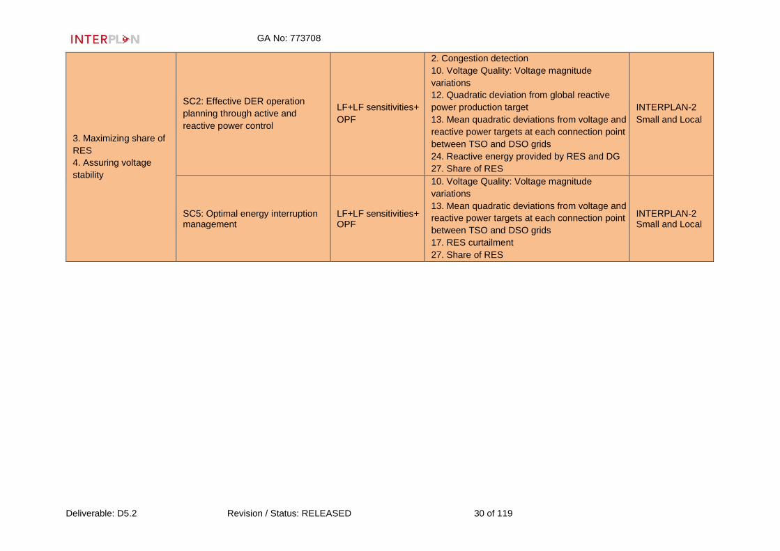
3. Maximizing share of
RES
4. Assuring voltage
stability
SC2: Effective DER operation
planning through active and
reactive power control
LF+LF sensitivities+
OPF
2. Congestion detection
10. Voltage Quality: Voltage magnitude
variations
12. Quadratic deviation from global reactive
power production target
13. Mean quadratic deviations from voltage and
reactive power targets at each connection point
between TSO and DSO grids
24. Reactive energy provided by RES and DG
27. Share of RES
INTERPLAN-2
Small and Local
SC5: Optimal energy interruption management
LF+LF sensitivities+ OPF
10. Voltage Quality: Voltage magnitude
variations
13. Mean quadratic deviations from voltage and
reactive power targets at each connection point
between TSO and DSO grids
17. RES curtailment
27. Share of RES
INTERPLAN-2 Small and Local

GA No: 773708
Deliverable: D5.2 Revision / Status: RELEASED 31 of 119
4.3 Stage 2 - Grid model selection/preparation
Stage 2 of the INTERPLAN tool is dedicated to the selection of the grid model, and the related
preparation, the latter according to the scenario selected under stage 1. The flowchart showing the
detailed steps to be performed by the user under stage 2 is shown in the figure below.
Figure 4: Stage 2 of INTERPLAN tool
When starting stage 2, the user has already selected the planning criteria, simulation functionalities,
the KPIs and the future scenario in stage 1. Stage 2 consists of the following steps:
• Step 2.1: Selection of the type of grid to be investigated. Here, the user can select among
three types of grid:
o Transmission grid only;
o Distribution grid only;
o Transmission and distribution grids.

GA No: 773708
Deliverable: D5.2 Revision / Status: RELEASED 32 of 119
• Step 2.2: Selection/insertion of the grid model(s). Here the user can select a benchmark
grid model or insert an own grid model. Alternatively, the user can do both these actions, for
instance, selecting a benchmark grid model representing a transmission grid and inserting
an own grid model representing a distribution grid, or vice versa.
• Step 2.3: Evaluation if a grid equivalent model is required. In this evaluation phase, the user
will be guided by the user manual showing when a grid equivalent is required. These
requirements are use-cases and showcases-oriented and are shown in Table 8.
In case any of these requirements is satisfied, the user directly goes to the step 2.5. In case
one of these requirements is satisfied, the user has to proceed with a grid equivalent model.
At this point, there are two possibilities excluding each other:
• Step 2.3.1: Choice of a grid equivalent from the grid equivalents library, constituted
by a number of pre-defined grid equivalents divided in three categories:
o Basic grid equivalents - simple representation of the grid focusing mainly on
preserving voltage, active and reactive power characteristics;
o Advanced grid equivalents - more complex representation considering also
different voltage levels and equivalenting different grid areas;
o Dynamic grid equivalents - simple or advanced grid equivalents suitable for
transient stability studies.
More details on these grid equivalents can be found in deliverable D4.2 [3].
This step is performed only in case the user finds the suitable grid equivalent from
the library. This library in fact consists of pre-defined grid equivalents built up on
benchmark grid models. Therefore, this step is performed only in case the user has
selected a benchmark grid model in step 2.2, for which – according to step 2.3 – a
grid equivalent is required.
• Step 2.3.2: Generation of a grid equivalent model. This step is performed in case the
user has inserted his own grid model in step 2.2, for which, according to step 2.3, a
grid equivalent is required. Under this step, the user will be provided with a grid
equivalent model through the Grid Equivalenting generation procedure which is a
module available in the tool. The procedure to generate grid equivalents takes as
inputs the original grid (transmission and/or distribution), and the KPIs that need to
be considered, that is, what the grid equivalent would be used for. Notice that for the
grid equivalent to be meaningful, the grid model provided by the user has to be similar
to the grids used to develop and train the grid equivalent procedure. More details on
the grid equivalenting approach can be found in deliverable D4.2 [3].
Note that in Step 2.3 and thus in Step 2.3.1 or in Step 2.3.2, the enabled choices are use case- and
showcase oriented according to the pre-defined schemes presented in the tables below, which are
part of the User Manual for stage 2 of INTERPLAN tool.
GA No: 773708
Deliverable: D5.2 Revision / Status: RELEASED 33 of 119
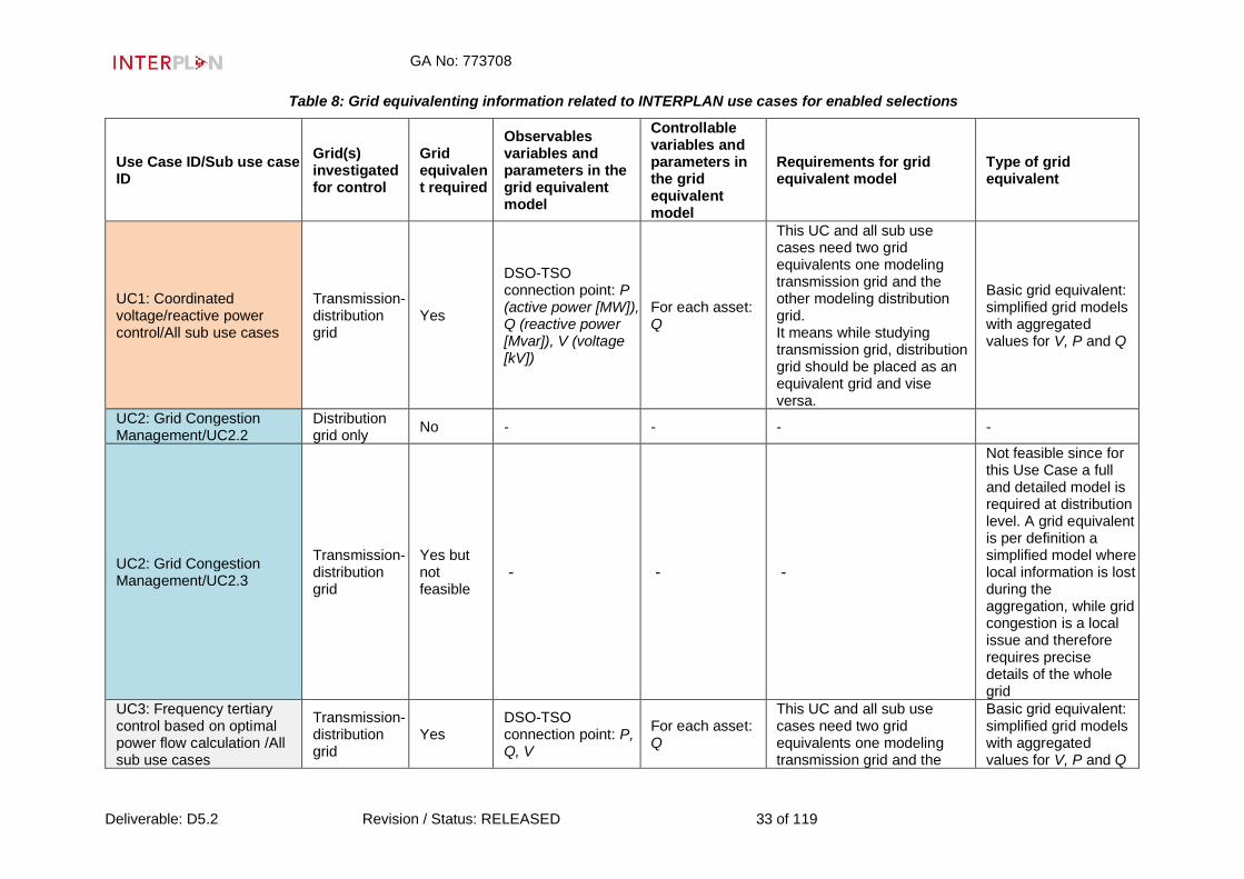
Table 8: Grid equivalenting information related to INTERPLAN use cases for enabled selections
Use Case ID/Sub use case ID
Grid(s) investigated for control
Grid equivalent required
Observables variables and parameters in the grid equivalent model
Controllable variables and parameters in the grid equivalent model
Requirements for grid equivalent model
Type of grid equivalent
UC1: Coordinated voltage/reactive power control/All sub use cases
Transmission-distribution grid
Yes
DSO-TSO connection point: P (active power [MW]), Q (reactive power [Mvar]), V (voltage [kV])
For each asset: Q
This UC and all sub use cases need two grid equivalents one modeling transmission grid and the other modeling distribution grid. It means while studying transmission grid, distribution grid should be placed as an equivalent grid and vise versa.
Basic grid equivalent: simplified grid models with aggregated values for V, P and Q
UC2: Grid Congestion Management/UC2.2
Distribution grid only
No - - - -
UC2: Grid Congestion Management/UC2.3
Transmission-distribution grid
Yes but not feasible
- - -
Not feasible since for this Use Case a full and detailed model is required at distribution level. A grid equivalent is per definition a simplified model where local information is lost during the aggregation, while grid congestion is a local issue and therefore requires precise details of the whole grid
UC3: Frequency tertiary control based on optimal power flow calculation /All sub use cases
Transmission-distribution grid
Yes DSO-TSO connection point: P, Q, V
For each asset: Q
This UC and all sub use cases need two grid equivalents one modeling transmission grid and the
Basic grid equivalent: simplified grid models with aggregated values for V, P and Q

GA No: 773708
Deliverable: D5.2 Revision / Status: RELEASED 34 of 119
other modeling distribution grid. It means while studying transmission grid, distribution grid should be placed as an equivalent grid and vise versa.
UC4: Fast Frequency Restoration Control / All sub use cases
Transmission-distribution grid
Yes
For each assets: Pmax, Pmin, Pactual, droop contribution; For each control area: Total grid frequency, droop contribution; Frequency; Tie-line active power flow among control areas
For each asset: P
The grid equivalent should keep the following information: • Total grid freq. droop contribution for each control area; • Tie-line active power flow among control areas.
Dynamic grid equivalents for each control area
UC5: Power balancing at DSO level /All sub use cases
Transmission-distribution grid
Yes DSO-TSO connection point: P, Q, V
None
This UC and all sub use cases need a grid equivalent for transmission network. The grid equivalent has to contain data on P, Q and V at the TSO-DSO connection point.
Basic grid equivalent: simplified grid models with aggregated values for V, P and Q
UC6: Inertia management /All sub use cases
Transmission-distribution grid
Yes
DSO-TSO connection point: P, Q, V Inertia
P for all units and internal DSL model parameters
This UC case and all sub use cases can use grid equivalent for both transmission and distribution network.
Dynamic grid equivalent
UC7: Optimal generation scheduling and sizing of DER for energy interruption management / All sub use cases
Transmission-distribution grid
Yes DSO-TSO connection point: P, Q, V and I
None
The equivalent for the LV feeder and MV feeder is required for the network preparation.
Advanced grid equivalent: The equivalent is representative of the static topology of the network inferred from the clustering parameter selection: Z_sum (Equivalent sum impedance per feeder [Ohm])

GA No: 773708
Deliverable: D5.2 Revision / Status: RELEASED 35 of 119
dPn/dPl (Maximum loading [%] Vn/Vl (Feeder maximal voltage drop [%])
Table 9: Grid equivalenting information related to INTERPLAN showcases for enabled selections
Showcase ID Grid(s) investigated for control
Grid equivalent required
Observables variables and parameters in the grid equivalent mode
Controllable variables and parameters in the grid equivalent model
Requirements for grid equivalent model
Type of grid equivalent
SC1: Low inertia systems
Transmission-distribution grid
Yes
DSO-TSO connection point: P, Q, V, Inertia; For each assets: Pmax, Pmin, Pactual, droop contribution; For each control area: Total grid frequency, droop contribution; Frequency; Tie-line active power flow among control areas
P for all units and internal DSL model parameters
This SC may need grid equivalent for both transmission and distribution network. The grid equivalent should keep following requirements: • Total grid freq. droop contribution per each control area; • Tie-line active power flow among control areas; • Inertia per each control area
Dynamic grid equivalents for each control area
SC2: Effective DER operation planning through active and reactive power control
Transmission-distribution grid
Yes but not feasible
- - -
Not feasible since for Use Case 2 on grid congestion management, which is part of this showcase, a full and detailed model is required at distribution level.

GA No: 773708
Deliverable: D5.2 Revision / Status: RELEASED 36 of 119
SC3: TSO-DSO power flow optimization
Transmission-distribution grid
Yes DSO-TSO connection point: P, Q, V
For each asset: P, Q
This SC needs two grid equivalents one modeling transmission grid and the other modeling distribution grid. It means while studying transmission grid, distribution grid should be placed as a grid equivalent and vise versa.
Basic grid equivalent: simplified grid models with aggregated values for V, P and Q.
SC4: Active and reactive power flow optimization at transmission and distribution networks
Transmission-distribution grid
Yes DSO-TSO connection point: P, Q, V
For each asset: P, Q
This SC needs two grid equivalents one modeling transmission grid and the other modeling distribution grid. It means while studying transmission grid, distribution grid should be placed as a grid equivalent and vise versa.
Basic grid equivalent: simplified grid models with aggregated values for V, P and Q
SC5: Optimal energy interruption management
Transmission-distribution grid
Yes
DSO-TSO connection point: P, Q, V and I
None
The equivalent for the LV feeder and MV feeder is required for the network preparation.
Advanced grid equivalent: The equivalent is representative of the static topology of the network inferred from the clustering parameter selection: Z_sum (Equivalent sum impedance per feeder [Ohm]) dPn/dPi (Maximum loading [%]) Vn/Vl (Feeder maximal voltage drop [%])

GA No: 773708
Deliverable: D5.2 Revision / Status: RELEASED 37 of 119
• Step 2.4: Application of a grid equivalent. This step is performed only in case the output from
step 2.3 is that a grid equivalent is required. Therefore, only after steps 2.3.1 or 2.3.2, the
user can enter this step.
• Step 2.5: Application of the scenario selected in Stage 1 to the grid model. In this step, the
INTERPLAN scenario chosen in the previous stage of the tool is adapted to the grid model
through the Scenario Adaptation procedure. In the most simple case, the step first
assesses the installed generation and load powers present in the grid model, finding an
operation point for generation and load which would result in a stable grid operation state
(e.g. all voltages and loadings within permitted limits). After that, the installed powers are set
into relation to according installed powers for the same region as given by the scenario. Using
this relation, individual generator and load nominal powers as well as found operation points
are scaled to match the scenario power. Also, grid reinforcements planned for the scenario
year (typically available for the extra high voltage (EHV) level only) are applied to the grid
model. After this, the LF calculation is repeated; in case it does not result in an allowed grid
operation state any more, manual reinforcement of the grid (typically HV, MV and LV levels)
is applied, or generator active and/or reactive powers are modified such as to find a valid
new operation point. A more sophisticated approach for this step could involve cost
calculation for the latter grid reinforcements and selection of the most cost-effective option.
Another possible refinement is to consider exact placement of new generators (typically RES)
in the scenario network, but this is only possible if according scenario data is at all available.
The step 2.5 is accessible from both step 2.4 or step 2.3 the latter in case a grid equivalent
model is not required.
• Step 2.6: Set the time-step. In this step, the user sets the time-step for the simulation phase
of stage 3.
• Step 2.7: Assignment of the time-series data: In this step, the time-series data are assigned
to the grid model(s) adapted to the chosen scenario and time step, through the time series
generation procedure, which is a module available in the tool. This procedure can be used
for any grid model that fulfils the following requirements [4]:
o For generator time series, the generation type (e.g. PV, onshore wind, offshore wind,
coal, nuclear) should be indicated by plant category (and subcategory in case of wind
turbines).
o Each generation type, including wind and PV generation, must be represented in the
grid model by separate generators. Separating wind and PV generation from loads is
recommended, otherwise they cannot be taken into account. The nominal power of
the generators should be given.
o The grid model should distinguish between onshore and offshore wind generation,
otherwise they will be treated as onshore wind generation.
o All loads are treated as scalable.
o Synchronous generators are used for balancing. The minimum and maximum active
power of each balancing generator should be given.
If all these requirements are met, time series can be generated for loads and generators. The
geographic locations of generation units are not relevant for this.
To give a practical example on how this procedure works, it is briefly explained below for a
specific grid model, i.e., SimBench-based grid model, used in the simulation of some of the
base showcases. The profiles for wind (onshore and offshore) generation, PV and demand
have been extracted from 50Hertz and ENTSO-E databases that are available online and
are given in p.u. which means that they can be scaled according to specific grid. Those data

GA No: 773708
Deliverable: D5.2 Revision / Status: RELEASED 38 of 119
are for the part of the German network operated under 50Hertz and represent year 2018.
Obtained profiles are being kept in a separate file which allows usage of any other profiles
that may be needed. Based on aforementioned data, 365 daily profiles were created with a
time step of 15 min. After choosing profiles from the initial model (at t=x) the base model is
created (at t=0). Then, from that model, time series data are adjusted for each time step
within a 24h period (including balancing). For each time step, an LF is performed to check
convergence.
This step 2.7 is the final one for Stage 2.
4.4 Stage 3 – Simulation & Evaluation
The stage 3 of INTERPLAN tool is dedicated to the simulation phase followed by the evaluation from
the user. In this stage, the Python-based toolbox interfaces with PowerFactory for simulating the
control functions embedded within INTERPLAN use cases and showcases. The flowchart showing
the detailed steps to be performed by the user under stage 3 is shown in the figure below.
Figure 5: Stage 3 of INTERPLAN tool
Before starting stage 3, the user has already selected the planning criteria, simulation functionalities,
the KPIs and the future scenario in stage 1, and has prepared the grid model(s) for simulation in
stage 2. When stage 3 starts, the user has two possibilities, i.e., performing simulations directly (step
3.0), or proceeding with one of the INTERPLAN solutions as control functions embedded in the
INTERPLAN use cases and showcases (step 3.1). The steps 3.0 and 3.1 exclude each other.
Therefore, this stage consists of the following steps:
• Step 3.0: Choice of performing simulations directly. This step is included for giving the
possibility to the user to create an own reference case, allowing to compare the results
attained by selecting one of the INTERPLAN solutions. This choice requires that the user
performs the simulations in consistence with the selections done in the previous stages 1
and 2.

GA No: 773708
Deliverable: D5.2 Revision / Status: RELEASED 39 of 119
• Step 3.1: Selection of INTERPLAN solution. In this step, the user selects one of the
INTERPLAN solutions enabled. In fact, based on the selections done in the previous stages,
only some (at least one) of the INTERPLAN solutions are enabled for this selection. The
INTERPLAN solutions are intended as the control functions embedded within
INTERPLAN use cases and showcases.
• Step 3.2: Simulation phase. At this step, the Pyhton-based toolbox interfaces with
PowerFactory for the simulation phase. In detail, the user can enter here either from step 3.0
or from step 3.1. In this latter case, the Python script code related to the control function
embedded within the INTERPLAN solution selected at step 3.1 is called in PowerFactory for
simulation.
• Step 3.3: Evaluation phase through KPI(s). In this step, the user evaluates the KPI(s) found
based on the own expertise and experience. Therefore, based on the values of the KPI(s)
found through simulations at Step 3.2, the user has two possibilities, thereby going to step
3.3.1 or 3.3.2 which exclude each other.
o Step 3.3.1. The user is satisfied with the KPI(s) found. In this case, this step
represents the final one for the entire tool.
o Step 3.3.2. The user is not satisfied with the KPI(s) found. In this case, the user goes
to the next step 3.4.
• Step 3.4. Decision to investigate other INTERPLAN solutions (use cases/control functions
under the same planning criterion or showcases/control functions addressing the same group
or sub-group of planning criteria. If entering this step, the user comes back to stage 1. In fact,
as already mentioned, most of the selections under stages 1, 2 and 3 are use cases- and
showcases-oriented according to the Tables 5-9.
The entire tool continues iteratively, until the condition under Step 3.1.1 is satisfied.
GA No: 773708
Deliverable: D5.2 Revision / Status: RELEASED 40 of 119
5. Simulation of grid equivalents for base showcases The INTERPLAN base showcases (BSCs) are described in detail in deliverable D5.1 [1].
A base showcase is defined as a combination of sub base use case(s) with no planning criteria and
no controllers for emerging technologies, such as RES, DG, demand response or storages. Base
showcases consist of base sub use cases, described for each use case in deliverable 3.2 [2], and
allow to analyze the operation challenges of the related use case(s). For each showcase, there is a
relevant base showcase with the same grid model, scenario, KPIs, simulation environment,
simulation type and time-series data. The simulation of base showcases is a key aspect to evaluate
effectiveness, reliability and robustness of the control functions proposed in the associated
showcases, which will be developed and implemented later in the project.
The five BSCs of INTERPLAN are associated to the following showcases [1]:
1. Low inertia systems;
2. Effective DER operation planning through active and reactive power control;
3. TSO-DSO power flow optimization;
4. Active and reactive power flow optimization at transmission and distribution networks;
5. Optimal energy interruption management
In the simulations, three grid models are used, i.e.:
• Cyprus grid model: a part of the real transmission/distribution grid including three different
substations (used for BSC1)
• SimBench-based grid model, which is a synthetic benchmark grid (used for BSC 2, 3 and 4).
Further details on this grid model can be found in deliverable D6.1 [4].
• Synthetic grid model provided by AIT (used for BSC5).
Where needed, basic grid equivalents are used. The basic grid equivalents represent the complex
grids in a simple model by only considering basic characteristics like connection node voltages and
reactive and active power values. These can be achieved by scaling up of most representative
feeders based on grid clustering (see deliverable D4.1 [5]). Thus, the resulting grid equivalent should
look like a small network model with one or more feeders depending on the different identified
feeder/network classes. The details related to the approach for generating basic grid equivalents can
be found in deliverable D4.2 [3].
In order to perform these simulations, a proper test case for each base showcase is defined. A test
case is meant as a specification of the inputs, execution conditions, testing procedure, and results
that define a single test to be executed in order to achieve a particular testing objective.
In the following, for each INTERPLAN base showcase, the detailed properties are first discussed.
Then, the test case properties are defined, and the results of the simulations are presented and
discussed. The KPIs are evaluated for creating a comparison with the associated showcases in order
to verify the effectiveness of future INTERPLAN embedded control functions. Then, the main
operation criticalities found in simulations as well as the possible solutions to apply through control
functions are presented.

GA No: 773708
Deliverable: D5.2 Revision / Status: RELEASED 41 of 119
5.1 Low inertia systems - BSC1 5.1.1 Base showcase properties
ID BSC_1
Associated Showcase SC_1 Low inertia systems
Base showcase description
For a given time of the day, the total system inertia is calculated based on available inertia from the rotating masses. Next, the biggest possible outage (generator/load) is determined by scanning operating units and synchronous tie lines as well as loads. Then, a frequency stability analysis is performed through a dynamic simulation, where the event is triggered by the outage defined in the previous step. The output of this base showcase is a set of information for each time step about system frequency stability as well as available and minimal required inertia.
Sub base use cases involved - associated use cases
4.1 - Fast Frequency Restoration Control 6.1 - Inertia management
No controllers are available. This sub-use case evaluates the network frequency response under specific instability events.
Only inertia from spinning masses of generators is available.
Sequence diagram

GA No: 773708
Deliverable: D5.2 Revision / Status: RELEASED 42 of 119
Timing diagram
Sequence of actions
Step n. Event name Event description
Information Exchange (if any)
Information producer (actor/tool)
Information receiver (actor/tool)
Information Exchanged IDs
1 Calculation of system inertia
Forecast data are read and system inertia is calculated
Forecast unit Calculation tool IEX_01
2 Determination of maximum possible outage
Maximum possible outage is found
Calculation tool Calculation tool IEX_02
3 Calculation of minimum needed inertia
Minimum needed system inertia is calculated
Calculation tool TSO IEX_03
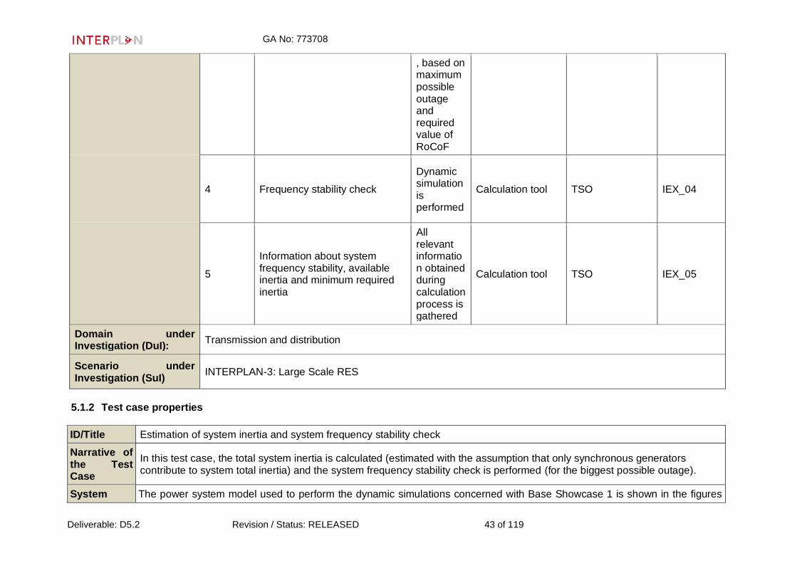
GA No: 773708
Deliverable: D5.2 Revision / Status: RELEASED 43 of 119
, based on maximum possible outage and required value of RoCoF
4 Frequency stability check
Dynamic simulation is performed
Calculation tool TSO IEX_04
5
Information about system frequency stability, available inertia and minimum required inertia
All relevant information obtained during calculation process is gathered
Calculation tool TSO IEX_05
Domain under Investigation (DuI):
Transmission and distribution
Scenario under Investigation (SuI)
INTERPLAN-3: Large Scale RES
5.1.2 Test case properties
ID/Title Estimation of system inertia and system frequency stability check
Narrative of the Test Case
In this test case, the total system inertia is calculated (estimated with the assumption that only synchronous generators contribute to system total inertia) and the system frequency stability check is performed (for the biggest possible outage).
System The power system model used to perform the dynamic simulations concerned with Base Showcase 1 is shown in the figures

GA No: 773708
Deliverable: D5.2 Revision / Status: RELEASED 44 of 119
under Test SuT)
below. The particular system comprises of five electrically connected areas.
Three transmission substations with same electrical specifications are included, which are
• Transmission Substation 1/Transmission Substation 2/ Transmission Substation 3: with two feeders each where two HV to MV transformers of 100 MVA respectively serves the distribution side. Each of the substation serves at the MV side

GA No: 773708
Deliverable: D5.2 Revision / Status: RELEASED 45 of 119
(11kV) load whereas PV, BESS (storage) and potentially EVs are connected2.
2The aggregated units (loads and PV systems) connected directly to the substation bus can be considered as specific type of basic grid equivalents. They are passive and they
do not reflect interactions between the various constituting elements. These will be elaborated further in the project with replacements that will be active and responsive to grid
state / needs according to the control functions associated to this showcase and highlight the importance of the equivalenting in the dynamic studies of the grid.

GA No: 773708
Deliverable: D5.2 Revision / Status: RELEASED 46 of 119
Generation Plant area:
• Two parallel slack node synchronous machines operate for a total of 50 MVA each. The power provided by the generators is produced at the voltage level of 11 kV and delivered into the 132 kV transmission network, through two 100 MVA transformers.

GA No: 773708
Deliverable: D5.2 Revision / Status: RELEASED 47 of 119
Wind farm area:
• includes one 16 MVA transformer and two wind turbine generators (WTG).

GA No: 773708
Deliverable: D5.2 Revision / Status: RELEASED 48 of 119
Objects under Test (OuT)
• Static Generators-2 wind turbine generators (23.57 MVA each)
• Load - 3 loads (user defined models-63.10 MW (area1) -31.65 MW (area2)-25.2 MW (area3))
• PV systems - 3 aggregated PV systems (user defined models)
• Synchronous Generators - 2 x 50 MVA each (Automatic Voltage Regulator Type: EXAC4, Speed Governor Type: TGOV1)
Function(s) under Test (FuT)
• Balanced LF Analysis
• Electromechanical Time Domain Dynamic Simulations (RMS)
Purpose of Test Case
The purpose of this test case is to serve as a reference case for Low inertia systems showcase 1. The values of the KPIs obtained for this test case will allow to validate the effectiveness of the control functions introduced in related showcase 1.
Time-series data
Generation/demand profiles for all generators (synchronous generators, PVs, wind turbines) and loads are available for a 24 h period. Battery energy storage systems (BESS) are assumed to be not used in a test case. The profile is presented in the figure below. Time-series data: synthetic Time frame: 24 h Time resolution: 15 min.
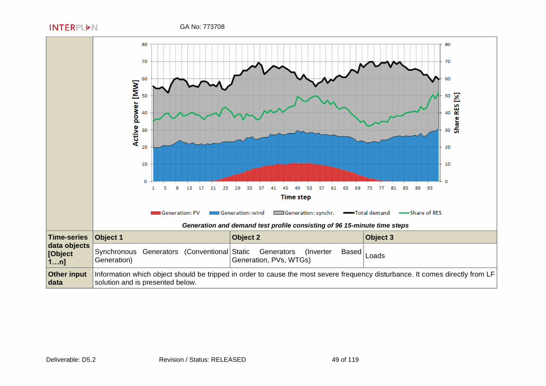
GA No: 773708
Deliverable: D5.2 Revision / Status: RELEASED 49 of 119
Generation and demand test profile consisting of 96 15-minute time steps
Time-series data objects [Object 1…n]
Object 1 Object 2 Object 3
Synchronous Generators (Conventional Generation)
Static Generators (Inverter Based Generation, PVs, WTGs)
Loads
Other input data
Information which object should be tripped in order to cause the most severe frequency disturbance. It comes directly from LF solution and is presented below.

GA No: 773708
Deliverable: D5.2 Revision / Status: RELEASED 50 of 119
Load and generation units with highest power consumption / production in each time interval
KPI under test
ID Name Formula
5 Frequency restoration control effectivity 𝐹𝑟𝑒𝑠𝑡𝑜𝑒𝑟𝑑 − 𝐹𝑛𝑜𝑚 ≤ 𝜀, 𝜀
→ 0
14
Level of DG / DRES utilization for ancillary services
𝑈𝐴𝑆%
= 𝐸𝐴𝑆
𝐸𝑡𝑜𝑡𝑎𝑙
∗ 100 [%] 𝐸𝐴𝑆 − 𝑡ℎ𝑒 𝑒𝑛𝑒𝑟𝑔𝑦 𝑢𝑠𝑒𝑑 𝑓𝑜𝑟 𝑎𝑛𝑐𝑖𝑙𝑙𝑎𝑟𝑦 𝑠𝑒𝑟𝑣𝑖𝑐𝑒𝑠 [𝑀𝑊ℎ] 𝐸𝑡𝑜𝑡𝑎𝑙 − 𝑡ℎ𝑒 𝑡𝑜𝑡𝑎𝑙 𝑒𝑛𝑒𝑟𝑔𝑦 𝑝𝑟𝑜𝑑𝑢𝑐𝑒𝑑 [𝑀𝑊ℎ]

GA No: 773708
Deliverable: D5.2 Revision / Status: RELEASED 51 of 119
20 Frequency nadir/zenith
𝑚𝑎𝑥(|𝑓𝑛 − 𝑓|) [𝐻𝑧] 𝑓𝑛 − 𝑛𝑜𝑚𝑖𝑛𝑎𝑙 𝑓𝑟𝑒𝑞𝑢𝑒𝑛𝑐𝑦 [𝐻𝑧] 𝑓 − 𝑠𝑦𝑠𝑡𝑒𝑚 𝑓𝑟𝑒𝑞𝑢𝑒𝑛𝑐𝑦 [𝐻𝑧]
21 Rate of Change of Frequency (RoCoF)
𝑑𝑓
𝑑𝑡 =
𝑃𝑔 − 𝑃𝑙
2𝐻𝑠𝑦𝑠
𝑑𝑓
𝑑𝑡 − 𝑟𝑎𝑡𝑒 𝑜𝑓 𝑐ℎ𝑎𝑛𝑔𝑒 𝑜𝑓 𝑓𝑟𝑒𝑞𝑢𝑒𝑛𝑐𝑦 [𝐻𝑧
/𝑠] 𝑃𝑔 − 𝑔𝑒𝑛𝑒𝑟𝑎𝑡𝑜𝑟𝑠′ 𝑎𝑐𝑡𝑖𝑣𝑒 𝑝𝑜𝑤𝑒𝑟 [pu]
𝑃𝑙 − 𝑑𝑒𝑚𝑎𝑛𝑑 𝑎𝑐𝑡𝑖𝑣𝑒 𝑝𝑜𝑤𝑒𝑟 [𝑝𝑢] 𝐻𝑠𝑦𝑠 − 𝑠𝑦𝑠𝑡𝑒𝑚 𝑖𝑛𝑒𝑟𝑡𝑖𝑎 [𝑠]
25 Indication of Stability No calculation needed; this KPI is a boolean variable (YES/NO)
26 Oscillation damping
𝜎 = ln(𝑝1
𝑝2)
𝑝1, 𝑝2 − 𝑚𝑎𝑥 𝑣𝑎𝑙𝑢𝑒𝑠 𝑜𝑓 𝑡𝑤𝑜 𝑐𝑜𝑛𝑠𝑒𝑐𝑢𝑡𝑖𝑣𝑒 𝑠𝑤𝑖𝑛𝑔𝑠 𝑜𝑓 𝑡ℎ𝑒 𝑠𝑖𝑔𝑛𝑎𝑙
27 Share of RES
𝑅𝐸𝑆% = 𝑃𝑅𝐸𝑆
𝑃𝑡𝑜𝑡𝑎𝑙 ∗ 100 [%]
𝑃𝑅𝐸𝑆 𝐴𝑐𝑡𝑖𝑣𝑒 𝑝𝑜𝑤𝑒𝑟 𝑝𝑟𝑜𝑣𝑖𝑑𝑒𝑑 𝑏𝑦 𝑅𝐸𝑆 𝑎𝑡 𝑎 𝑔𝑖𝑣𝑒𝑛 𝑡𝑖𝑚𝑒 𝑠𝑡𝑒𝑝 [𝑀𝑊] 𝑃𝑡𝑜𝑡𝑎𝑙 𝑇𝑜𝑡𝑎𝑙 𝑎𝑐𝑡𝑖𝑣𝑒 𝑝𝑜𝑤𝑒𝑟 𝑝𝑟𝑜𝑣𝑖𝑑𝑒𝑑 𝑏𝑦 𝑅𝐸𝑆 𝑎𝑛𝑑 𝑛𝑜𝑛 𝑅𝐸𝑆 𝑔𝑒𝑛𝑒𝑟𝑎𝑡𝑜𝑟𝑠 𝑎𝑡 𝑎 𝑔𝑖𝑣𝑒𝑛 𝑡𝑖𝑚𝑒 𝑠𝑡𝑒𝑝 [𝑀𝑊]
Variability attributes (test factors)
No system parameters are varied
Quality attributes
RoCoFmax = 1 Hz/s fmin such that no protection is triggered, in particular no under-frequency load shedding (UFLS) is initiated (system dependent setting)

GA No: 773708
Deliverable: D5.2 Revision / Status: RELEASED 52 of 119
fmax such that no protection is triggered, in particular no generation overfrequency protection is initiated
Simulation environment
DIgSILENT PowerFactory
Simulation type
Dynamic (Time Domain Electromechanical Simulations) & Semi-Dynamic
Output parameters
System Frequency (f), RoCoF (df/dt), active power (P) (generators, storages, loads), voltages (V)
Initial system state
Steady state
Evolution of system state and test signals
Outage of generation unit (Synchronous generation or Static Generation) or load which generates or consumes the highest amount of power at a given time step
Other parameters
Total system inertia, needed system inertia, settling frequency, frequency nadir/zenith
Storage of data
PowerFactory (*.pfd), (*.csv),
Temporal resolution
15 minutes within 24 hours in total
Source of uncertainty
Time-series data
Suspension criteria / Stopping criteria
No convergence in LF Error in initialization of dynamic simulation (models do not initialize, error in performing inversion matrix in dynamic simulations) Initial conditions cannot be calculated.
5.1.3 Test case results
ID/Title BSC1
KPI evaluation ID Name Value

GA No: 773708
Deliverable: D5.2 Revision / Status: RELEASED 53 of 119
5 Frequency restoration control effectivity
Out of 96 time domain simulations where generation is tripped in 75 the frequency is restored (78%), Out of 96 time domain simulations where load is tripped in 90 the frequency is restored (94%). See results below for details.
14 Level of DG / DRES utilization for ancillary services
This KPI is zero for this BSC, since this BSC does not assume utilisation of DG/DRES for ancillary services as no controls are active.
26 Oscillation damping All cases are critically damped
20 Frequency nadir/zenith
Out of 96 time domain simulations where generation is tripped 69 is secure (72%), Out of 96 time domain simulations where load is tripped 84 is secure (88%). Secure cases are those that do not trip frequency protections, i.e. the nadir or zenith are above and below protection activation threshold respectively. See Results below for details.
21 Rate of Change of Frequency (RoCoF)
Out of 96 time domain simulations where generation is tripped 3 have maximum RoCoF >= -1 Hz/s (3%), Out of 96 time domain simulations where load is tripped 0 have maximum RoCoF <= 1 Hz/s (0%). See Results below for details.
25 Indication of Stability
Out of 96 time domain simulations where generation is tripped 75 is stable (78%), Out of 96 time domain simulations where load is tripped 90 is stable (94%). See Results for details.
27 Share of RES min. 31%, max. 52%

GA No: 773708
Deliverable: D5.2 Revision / Status: RELEASED 54 of 119
Results
The purpose of the SC “Low inertia systems” is to assure adequate level of inertia and proper frequency regulation throughout a given period of time. The methodology applied here consists in performing dynamic simulations for each time step of the time series data. Since both generation and system demand change in time, this BSC shows how these slow changes affect system stability evaluated by indices associated with dynamic (transient) phenomena. All results are presented in figure at right, in which each curve represents a frequency transient for different moment in time. The top group of curves is obtained for load trip, whereas the bottom part for generation trip. It is evident that in this BSC, in which only synchronous generation is equipped with frequency control, some curves, i.e. some operating points of the power system, are stable and some are not.
Results of dynamic simulations performed for each time step during 24
hours: frequency transients

GA No: 773708
Deliverable: D5.2 Revision / Status: RELEASED 55 of 119
As highlighted in the figure at right, the unstable cases for generation trip are marked with black colour. As can be noticed from the time bar below the plot, they are associated with relatively high generation from synchronous generators. If one of them is being tripped, the other one has insufficient active power reserve to cover up for the power loss and thus the whole case is unstable. Similarly, the unstable cases for load trip are marked with red colour. These instabilities manifest themselves when there is not enough range to decrease power generated by synchronous machines after the load is tripped. No overfrequency protection is modelled thus the frequency continues to increase. There are two times during the day when it happens, both when there is the highest share of RES.
Results of dynamic simulations performed for each time step during 24
hours: overfrequency instability (red) and underfrequency instability (black)

GA No: 773708
Deliverable: D5.2 Revision / Status: RELEASED 56 of 119
All unstable cases are insecure, but there are stable cases which are insecure as well. The insecurity comes from the fact that nadir or zenith of the frequency is at such a level that it would cause activation of frequency protection, thus proceeding disconnection of load or generation respectively. In this BSC safe range of frequency deviations was assumed to be ±2 Hz.
Results of dynamic simulations performed for each time step during 24 hours: overfrequency protection activation (red) and underfrequency
protection activation (black)
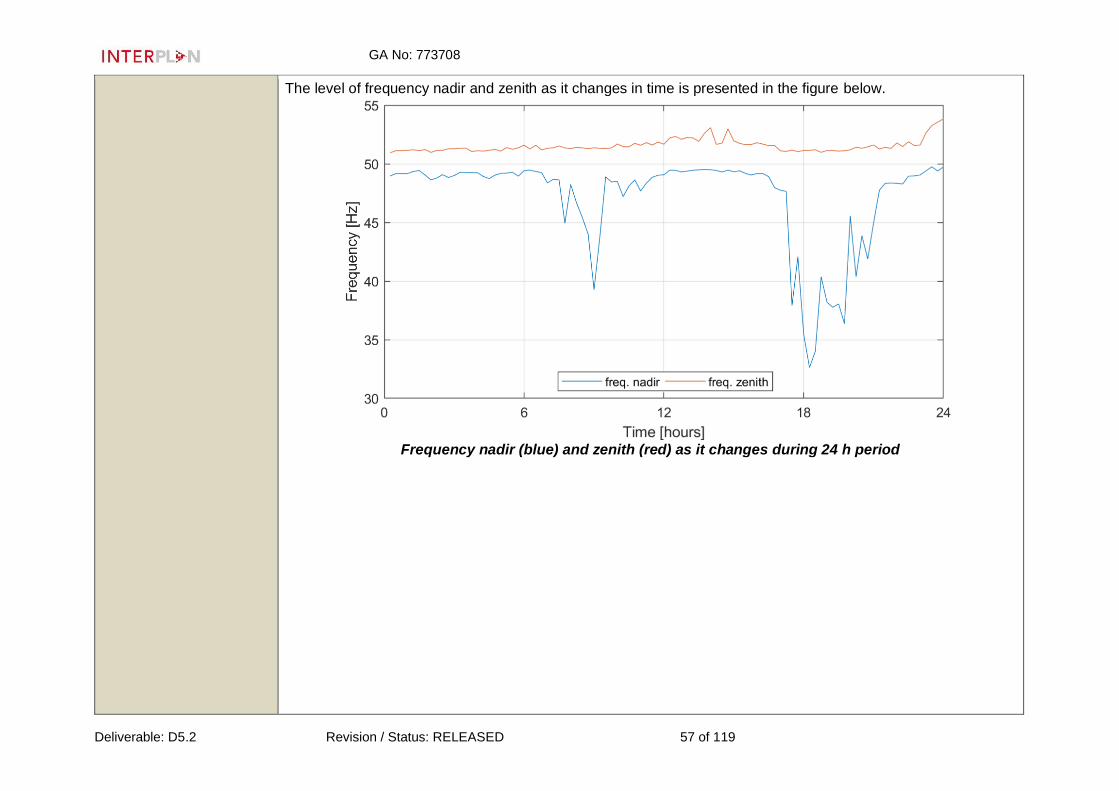
GA No: 773708
Deliverable: D5.2 Revision / Status: RELEASED 57 of 119
The level of frequency nadir and zenith as it changes in time is presented in the figure below.
Frequency nadir (blue) and zenith (red) as it changes during 24 h period

GA No: 773708
Deliverable: D5.2 Revision / Status: RELEASED 58 of 119
Operating conditions also affect system inertia and thus the RoCoF. RoCoF in this BSC is actually affected more by the fact that the size of power imbalance resulting from generation or load trip changes as the power system proceeds from one operating point to another. The figure below presents these changes, i.e. it shows values of RoCoF for generation trip (solid curves) and for load trip (dashed curves) for a particular moment in the time series. This figure also reveals the differences in RoCoF measured with different length of the sliding window. Slower protections might react to the 1000 ms window whereas the faster ones will use a 100 ms or 500 ms window. The security criterion applied here is that the RoCoF should not exceed ±1 Hz/s if measured with a 500 ms window.
Maximum RoCoF for generation trip (solid line) and load trip (dashed line) as it changes during 24 h
period
Network operation criticalities found
As mentioned in the Results section and as indicated by the KPIs, several system security criteria were not met. In particular, the criteria related to stability and security of operation returned a few cases in which they are not met. When this situation is improved, the next criterion in terms of importance is inadequate inertia measured by means of RoCoF.
Possible solutions identified
Since all results are highly reliant on the operating point of the power system, a measure to improve situation is to change the operating point of particular devices in particular moments during the analysed (planned) operation period. However, this should be considered as last resort not only because it collides with market solution of the

GA No: 773708
Deliverable: D5.2 Revision / Status: RELEASED 59 of 119
LF, but also because there are better means to do it. Firstly, synthetic inertia (SI) concept is going to be applied to available resources and secondly a new methodology for frequency control is going to be used . Thus by including novel dynamic control methods re-dispatching and/or curtailment costs can be avoided.
Remarks and open issues
In order to improve the accuracy of the results the dynamic model should be equipped with:
• load models implementing active power dependence on frequency, P=f(f) or P=f(f,t),
• under/overfrequency protection of the generating units,
• UFLS models for loads,
• frequency dependent characteristics of RES as required by the network codes (option).

GA No: 773708
Deliverable: D5.2 Revision / Status: RELEASED 60 of 119
5.2 Effective DER operation planning through active and reactive power control - BSC2 5.2.1 Base showcase properties
ID BSC_2
Associated Showcase
SC_2 - Effective DER operation planning through active and reactive power control
Base showcase description
For a given time step, DG and RES are uncontrolled. The congestion detection is performed at transmission level followed by an LF calculation. The network status at transmission level is analysed based on the active and reactive power information, evaluating also possible congestion problems. The voltage magnitude and angle are also checked.
Sub base use cases involved - associated use cases
2.1 - Grid congestion management 1.1 - Coordinated voltage/ reactive power control
In this sub-use case, the tool acts on TSO level for detecting possible congestion events for each time step.
The LF calculation is performed at TSO level to obtain the voltage, the reactive power information as well as power losses for each time step.
Sequence diagram

GA No: 773708
Deliverable: D5.2 Revision / Status: RELEASED 61 of 119
Timing diagram
Sequence of actions
Step n. Event name Event description
Information Exchange (if any)
Information producer (actor/tool)
Information receiver (actor/tool)
Information Exchanged IDs
1
Congestion Detection
TSO grid and forecast data for DG, RES and loads are read; therefore possible congestion problems in the transmission grid are detected
TSO grid information and forecast unit
Congestion detection function
IEX_01, IEX_02
2 LF calculation
An LF calculation is performed by the TSO to check the general status of the network while considering the detected congestion as well as load and generation forecast
TSO grid information and load and generation forecast unit
LF, TSO
IEX_01, IEX_02, IEX_03

GA No: 773708
Deliverable: D5.2 Revision / Status: RELEASED 62 of 119
data within the given horizon time.
Domain under Investigation (DuI):
Transmission grid
Scenario under Investigation (SuI)
INTERPLAN-2: Small and Local
5.2.2 Test case properties
ID/Title Evaluation of system congestion and reactive power of a transmission network
Narrative of the Test Case
This test case evaluates possible congestion scenarios in the power grid through a congestion detection function and the
general status of the network (e.g., voltage and reactive power) through an LF calculation.
System under Test (SuT)
The power system under test is a model based on SimBench. It is a synthetic benchmark grid and comprises the EHV (380 – 220 kV), HV (110kV), MV (20kV), and LV (400V) voltage levels. The model contains a total of 287 lines, 235 busbars, 15 transformers, 225 loads, and 257 static generators. The study is performed at transmission level.

GA No: 773708
Deliverable: D5.2 Revision / Status: RELEASED 63 of 119
Objects under Test (OuT)
• Static Generators (Wind, PVs, Hydro)
• Loads
• Synchronous Generators (Gas, Coal)
Function(s) under Test (FuT)
• “Congestion Detection” function
• LF function
Purpose of Test Case
The test is aimed to evaluate the "Congestion Detection" function of the UC2 whereas the LF calculation of UC1 runs to evaluate the general status of the network within the given time frame.
Time-series data
Generation/demand profiles for all generators (synchronous, PV, WTG) and loads are available for a 24h period. Type: synthetic Time frame: 24h Time resolution: 15 min

GA No: 773708
Deliverable: D5.2 Revision / Status: RELEASED 64 of 119
Time-series data objects [Object 1…n]
Object 1 Object 2 Object 3
Static Generator Synchronous Generator Loads
KPI under test
ID Name Formula
2 Congestion detection
Congestion = If abs( 𝑃𝑙𝑖𝑛𝑒_𝑖) > 𝑃𝑟𝑎𝑡𝑖𝑛𝑔_𝑙𝑖𝑛𝑒_𝑖 the line-i is congested.
𝑃𝑙𝑖𝑛𝑒_𝑖[kW] is the active power that flows troughs the line i
𝑃𝑟𝑎𝑡𝑖𝑛𝑔_𝑙𝑖𝑛𝑒_𝑖[kW] is the nominal active power of the line i
10 Voltage Quality
According to the defined EN 50160 Standards and VDE-AR-N 4120 bus bar voltage magnitudes
must comply with following allowed range of variation.
• LV, MV: (±10% of nominal voltage)
• HV & EHV: (±4-7% of nominal voltage)
Voltage deviation indices can be defined to find the frequency or duration that the bus bar
voltages violate the allowed voltage range.
• Number of voltage excursions exceeded n minutes per year
• Percentage of time that the transmission voltage exceeds the permissible limits
14
Level of DG / DRES utilization for ancillary services
𝑈𝐴𝑆% = 𝐸𝐴𝑆
𝐸𝑡𝑜𝑡𝑎𝑙 ∗ 100 [%]
𝐸𝐴𝑆 − 𝑡ℎ𝑒 𝑒𝑛𝑒𝑟𝑔𝑦 𝑢𝑠𝑒𝑑 𝑓𝑜𝑟 𝑎𝑛𝑐𝑖𝑙𝑙𝑎𝑟𝑦 𝑠𝑒𝑟𝑣𝑖𝑐𝑒𝑠 [𝑀𝑊ℎ] 𝐸𝑡𝑜𝑡𝑎𝑙 − 𝑡ℎ𝑒 𝑡𝑜𝑡𝑎𝑙 𝑒𝑛𝑒𝑟𝑔𝑦 𝑝𝑟𝑜𝑑𝑢𝑐𝑒𝑑 [𝑀𝑊ℎ]
13
Mean quadratic deviations from voltage and reactive power targets at each connection point between TSO and DSO grids
Let C be the set of connection points between TSOs and DSOs. Let qc,target (t) [kVar] be the target value for reactive power transmission from DSO to TSO at connection point c and time t, as e.g. calculated by grid operation planning. Let qc(t) be the reactive power actually provided from DSO to TSO at connection point c and time t. Then the KPI related to reactive power at time t is defined as: 1
|𝐶|∑(𝑞𝑐,𝑡𝑎𝑟𝑔𝑒𝑡(𝑡) − 𝑞𝑐(𝑡))
2
𝑐∈𝐶
The KPI related to voltage is defined as follows. Let uc,target [V] be the nominal value for the line-to-line voltage at connection point c, calculated as mean over all phases. Let uc(t) be the actual line-to-line voltage mean over all phases. Then, the KPI at time t is:

GA No: 773708
Deliverable: D5.2 Revision / Status: RELEASED 65 of 119
1
|𝐶|∑(𝑢𝑐,𝑡𝑎𝑟𝑔𝑒𝑡 − 𝑢𝑐(𝑡))
2
𝑐∈𝐶
1
Level of losses in transmission and distribution networks
𝑃𝑒𝑟𝑐𝑒𝑛𝑡𝑎𝑔𝑒 𝑜𝑓 𝑙𝑜𝑠𝑠𝑒𝑠
= 𝐴𝑚𝑜𝑢𝑛𝑡 𝑜𝑓 𝑖𝑛𝑗𝑒𝑐𝑡𝑒𝑑 𝑒𝑛𝑒𝑟𝑔𝑦 − 𝑎𝑚𝑜𝑢𝑛𝑡 𝑜𝑓 𝑒𝑛𝑒𝑟𝑔𝑦 𝑑𝑒𝑙𝑖𝑣𝑒𝑟𝑒𝑑 𝑡𝑜 𝑡ℎ𝑒 𝑐𝑢𝑠𝑡𝑜𝑚𝑒𝑟𝑠
𝐴𝑚𝑜𝑢𝑛𝑡 𝑜𝑓 𝑖𝑛𝑗𝑒𝑐𝑡𝑒𝑑 𝑒𝑛𝑒𝑟𝑔𝑦× 100
Variability attributes (test factors)
There are no variables to be varied
Quality attributes
Lines/transformers/generators are not overloaded (loading =< 90%)
Simulation environment
DIgSILENT PowerFactory
Simulation type
Semi-dynamic
Output parameters
Base Use Case 2: Line congested at TSO level - Base Use Case 1: reactive power and voltage
Initial system state
Steady state
Evolution of system state and test signals
Time series for this showcase have been designed in a way that a congestion event occurs at least in one time step.
Other parameters
Grid model data (e.g transmission line parameters)
Storage of data
PowerFactory (*.pfd), excel (*.xlsx, *.csv)
Temporal resolution
15 minutes within 24 hours

GA No: 773708
Deliverable: D5.2 Revision / Status: RELEASED 66 of 119
Source of uncertainty
Time-series data
5.2.3 Test case results
ID/Title Simulation results for BSC1 by using SimBench-based grid model
KPI evaluation
ID Name Value
2 Congestion detection 1 (boolean variable). See figure below for KPI 2 for more details.
10 Voltage Quality See figure below for KPI 10
13
Mean quadratic deviations from voltage and reactive power targets at each connection point between TSO and DSO grids
See figure below for KPI 13
14 Level of DG / DRES utilization for ancillary services
This KPI is zero for this BSC, since this BSC does not assume utilisation of DG/DRES for ancillary services as no controls are active.
1 Level of losses in transmission and distribution networks
See figure below for KPI 1 (evaluated only for transmission network)
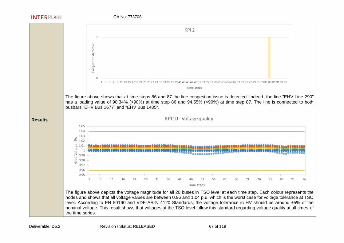
GA No: 773708
Deliverable: D5.2 Revision / Status: RELEASED 67 of 119
Results
The figure above shows that at time steps 86 and 87 the line congestion issue is detected. Indeed, the line "EHV Line 290" has a loading value of 90.34% (>90%) at time step 86 and 94.55% (>90%) at time step 87. The line is connected to both busbars "EHV Bus 1677" and "EHV Bus 1485".
The figure above depicts the voltage magnitude for all 20 buses in TSO level at each time step. Each colour represents the nodes and shows that all voltage values are between 0.96 and 1.04 p.u. which is the worst case for voltage tolerance at TSO level. According to EN 50160 and VDE-AR-N 4120 Standards, the voltage tolerance in HV should be around ±5% of the nominal voltage. This result shows that voltages at the TSO level follow this standard regarding voltage quality at all times of the time series.

GA No: 773708
Deliverable: D5.2 Revision / Status: RELEASED 68 of 119
The figure above depicts the voltage and reactive power deviation. The target value for voltage was set to 1 p.u.; for reactive power, it was set to zero. Moreover, for both formulations C, set of connection point, is 1 and the square root has been calculated for both. It shows that reactive power and voltage deviation from target values at the connection point are close to constant at off peak hours. At peak hours, the voltage (KPI13) has lower deviation from 1 p.u., while the reactive power shows higher deviation from zero. The reason of choosing zero for the reactive power target is to decrease the interaction among TSO and DSO.

GA No: 773708
Deliverable: D5.2 Revision / Status: RELEASED 69 of 119
The percentage of loss at TSO level is shown in the figure above for all time steps. The power loss in HV is usually lower than the values found for this simulation, where it varies between 1% to 2%. The maximum loss is foundat the time steps where the congestion event occurs. The power losses should decrease through the implementation of the control functions related to the SC2.
Network operation criticalities found
In the simulation of this base showcase, the following operation criticalities have been found:
• Congestion event found at transmission level;
• Power losses at TSO level for some time steps are considerable with regards to the average power losses at transmission level in Germany according to [6].
Possible solutions identified
In order to solve the issues in this simulation, the possible solutions identified are:
• Optimal active power re-dispatching among both TSO and DSO assets such as to obtain a loading value less than 90% for all lines in the grid model under consideration. This re-dispatching function can involve both resources connected at transmission level and flexibility resources connected at distribution level.
• Considering the optimal active power set-points re-dispatched to solve congestion events, an optimal power flow to minimize the power losses will be run in a way that optimum reactive power set points and voltage set points can be acquired.
These potential solutions related to the day-ahead operation planning will be implemented in the control functions related to SC2 “Effective DER operation planning through active and reactive power control”. A comparison will be made by considering these KPIs to show the effectiveness of the control functions in the SC2 in solving the operation issues identified for this BSC.

GA No: 773708
Deliverable: D5.2 Revision / Status: RELEASED 70 of 119
5.3 TSO-DSO power flow optimization - BSC3 5.3.1 Base showcase properties
ID BSC_3
Associated Showcase
SC_3 TSO-DSO power flow optimization
Base showcase description
For a given time step, an LF at the TSO level is calculated. Then, an LF at the DSO grid is calculated. As an output, information on a transmission and distribution grid state (power losses, etc.) is obtained.
Sub base use cases involved - associated use cases
3.1 - Power balancing at TSO level based on LF calculations 5.1 - Power balancing at DSO level
DSO does not participate in providing tertiary reserves. TSO performs LF calculations at its own network and distribution networks are considered as grids with no controllable active power.
DSO performs LF calculations at its network. No controllers for power flow optimization are available.
Sequence diagram

GA No: 773708
Deliverable: D5.2 Revision / Status: RELEASED 71 of 119
Timing diagram
Sequence of actions
Step n.
Event name Event description
Information Exchange (if any)
Information producer (actor/tool)
Information receiver (actor/tool)
Information Exchanged IDs
1 Read input data
Data on forecasted demand/generation are read.
Forecast unit Calculation tool IEX_01, IEX_02
2 LF at TSO level
LF is calculated for TSO grid Calculation tool TSO, DSO IEX_03
3 LF at DSO level
LFi s calculated for DSO grid Calculation tool TSO, DSO IEX_04

GA No: 773708
Deliverable: D5.2 Revision / Status: RELEASED 72 of 119
4 Information on LF
Information on LF at transmission and distribution grids are gathered.
TSO, DSO Controllable transmission-connected units
IEX_05
Domain under Investigation (DuI):
Transmission and distribution grid
5.3.2 Test case properties
ID/Title LF at transmission and distribution grids
Narrative of the Test Case
In this test case, LF for TSO and DSO grids are calculated to obtain the state of the grid (losses, etc). Resources at the DSO grid are considered to be uncontrollable.
System under Test (SuT)
The system under test is a grid model based on SimBench which has been divided into four areas (one TSO and three radial DSO networks). For both the base use cases, grid equivalents were created (DSO equivalents for BUC3 and TSO equivalents for BUC5). Those equivalents have been modelled as external grids (one for each TSO-DSO connection point), with power flow between TSO and DSOs maintained.

GA No: 773708
Deliverable: D5.2 Revision / Status: RELEASED 73 of 119
Objects under Test (OuT)
Synchronous generators, static generators, loads, TSO/DSO transformers, lines
Function(s) under Test (FuT)
LF
Purpose of Test Case
The purpose of this test case is to serve as a reference case for TSO-DSO power flow optimization showcase. Values of the given KPIs obtained for this test case will allow to show the effectiveness of controllers introduced in related showcase 3.
Time-series data
Generation/demand profiles for all generators (synchronous, PV, WTG) and loads (including EVs) are available for a 24h period. Storage systems are assumed to be not used in this test case. Type: synthetic Time frame: 24h Time resolution: 15 min
Time-series data Object 1 Object 2

GA No: 773708
Deliverable: D5.2 Revision / Status: RELEASED 74 of 119
objects [Object 1…n]
Generators Loads
Other input data Required tertiary control reserve
KPI under test
ID Name Formula
1 Level of losses in transmission and distribution networks
𝑃𝑙𝑜𝑠𝑠𝑒𝑠
= 𝑎𝑚𝑜𝑢𝑛𝑡 𝑜𝑓 𝑖𝑛𝑗𝑒𝑐𝑡𝑒𝑑 𝑒𝑛𝑒𝑟𝑔𝑦 − 𝑎𝑚𝑜𝑢𝑛𝑡 𝑜𝑓 𝑒𝑛𝑒𝑟𝑔𝑦𝑑𝑒𝑙𝑖𝑣𝑒𝑟𝑒𝑑 𝑡𝑜 𝑐𝑢𝑠𝑡𝑜𝑚𝑒𝑟𝑠
𝑎𝑚𝑜𝑢𝑛𝑡 𝑜𝑓 𝑖𝑛𝑗𝑒𝑐𝑡𝑒𝑑 𝑒𝑛𝑒𝑟𝑔𝑦
∗ 100 [%]
7 Power losses
𝑃𝑙𝑜𝑠𝑠𝑒𝑠 = ∑ |𝐼|𝑖2
𝑁𝑙𝑖𝑛𝑒
𝑖
∗ 𝑟𝑖 [𝑘𝑊] 𝐼𝑖 − 𝑚𝑎𝑔𝑛𝑖𝑡𝑢𝑑𝑒 𝑜𝑓 𝑐𝑢𝑟𝑟𝑒𝑛𝑡 𝑓𝑙𝑜𝑤 𝑖𝑛 𝑙𝑖𝑛𝑒 𝑖 [𝐴] 𝑟𝑖 − 𝑟𝑒𝑠𝑖𝑠𝑡𝑎𝑛𝑐𝑒 𝑜𝑓 𝑙𝑖𝑛𝑒 𝑖 [𝛺]
14 Level of DG / DRES utilization for ancillary services
𝑈𝐴𝑆% = 𝐸𝐴𝑆
𝐸𝑡𝑜𝑡𝑎𝑙 ∗ 100 [%]
𝐸𝐴𝑆 − 𝑡ℎ𝑒 𝑒𝑛𝑒𝑟𝑔𝑦 𝑢𝑠𝑒𝑑 𝑓𝑜𝑟 𝑎𝑛𝑐𝑖𝑙𝑙𝑎𝑟𝑦 𝑠𝑒𝑟𝑣𝑖𝑐𝑒𝑠 [𝑀𝑊ℎ] 𝐸𝑡𝑜𝑡𝑎𝑙 − 𝑡ℎ𝑒 𝑡𝑜𝑡𝑎𝑙 𝑒𝑛𝑒𝑟𝑔𝑦 𝑝𝑟𝑜𝑑𝑢𝑐𝑒𝑑 [𝑀𝑊ℎ]
16 Transformer loading 𝐿𝑜𝑎𝑑𝑖𝑛𝑔% =
𝑝𝑜𝑤𝑒𝑟 𝑎𝑡 𝑡𝑟𝑎𝑛𝑠𝑓𝑜𝑟𝑚𝑒𝑟 𝑝𝑟𝑖𝑚𝑎𝑟𝑦 𝑤𝑖𝑛𝑑𝑖𝑛𝑔
𝑡𝑟𝑎𝑛𝑠𝑓𝑜𝑟𝑚𝑒𝑟 𝑛𝑜𝑚𝑖𝑛𝑎𝑙 𝑝𝑜𝑤𝑒𝑟
∗ 100 [%]

GA No: 773708
Deliverable: D5.2 Revision / Status: RELEASED 75 of 119
17 RES curtailment
𝐶𝑢𝑟𝑡𝑎𝑖𝑙𝑚𝑒𝑛𝑡%
= 100 − 𝑒𝑛𝑒𝑟𝑔𝑦 𝑠𝑢𝑝𝑝𝑙𝑖𝑒𝑑 𝑏𝑦 𝑅𝐸𝑆 𝑡𝑜 𝑡ℎ𝑒 𝑔𝑟𝑖𝑑
𝑅𝐸𝑆 𝑎𝑣𝑎𝑖𝑙𝑎𝑏𝑙𝑒 𝑒𝑛𝑒𝑟𝑔𝑦
∗ 100 [%]
23 Mean quadratic deviations from active power targets at TSO/DSO connection points
1
|𝐶|∑(𝑃𝑐,𝑡𝑎𝑟𝑔𝑒𝑡(𝑡)
𝑐𝜖𝐶
− 𝑃𝑐(𝑡))2
Variability attributes (test factors)
No parameters are varied
Quality attributes Lines/transformers/generators/storages are not overloaded (loading =< 90%)
Simulation environment
DIgSILENT PowerFactory
Simulation type Semi-dynamic
Output parameters Active power of PV and WTG, sum of generation, EHV/HV transformers loading, power losses and loading on lines, bus voltages
Initial system state Steady state
Evolution of system state and test signals
No event required
Storage of data PowerFactory (*.pfd), excel (*.xlsx), xml
Temporal resolution
15 minutes within 24 hours in total
Source of uncertainty
Time-series data, demand response availability, etc.
Suspension criteria / Stopping criteria
LF/ OPF does not calculate

GA No: 773708
Deliverable: D5.2 Revision / Status: RELEASED 76 of 119
5.3.3 Test case results
ID/Title Simulation results for BSC3 by using the SimBench-based grid model
KPI evaluation
ID Name Value
1 Level of losses in transmission and distribution networks
See figure below for KPI 1 (evaluated only for transmission network)
7 Power losses See figure below for KPI 7
14 Level of DG / DRES utilization for ancillary services
This KPI is zero for this BSC, since this BSC does not assume utilisation of DG/DRES for ancillary services as no controls are active.
16 Transformer loading See figure below for KPI 16
17 RES curtailment
Time step 47 (30.04 MW) Time step 96 (27.62 MW) RES curtailment was equal to 0 MW for 94 out of 96 simulation time steps. The only two time steps where curtailing RES was necessary were time step 47 (30.04 MW) and time step 96 (27.62 MW). Calculations were made for DSO network.
23
Mean quadratic deviations from active power targets at TSO/DSO connection points
See figure below for KPI 23

GA No: 773708
Deliverable: D5.2 Revision / Status: RELEASED 77 of 119
Results
The percentage of loss at TSO level is shown in the figure above for all time steps. The power loss here is varying between 1.1 and 1.9 %. The power losses are expected to decrease later in SC3 through the implementation of the related control functions
The total active power losses at DSO level are shown in the figure above for all time steps.

GA No: 773708
Deliverable: D5.2 Revision / Status: RELEASED 78 of 119
The figure above shows the percentage loading of transformers at TSO-DSO connection point.
This figure above shows the active power deviation. The target value for active power is set to zero, since the aim is to reduce the power exchange among TSO and DSO . Moreover, for the formulations C, as connection point set, is 1 and the square root has been calculated eventually. As expected, at peak hours, the deviation from active power target is higher,

GA No: 773708
Deliverable: D5.2 Revision / Status: RELEASED 79 of 119
because more active power is exchanged among DSO and TSO at those hours.
Network operation criticalities found
In the simulation of this base showcase, the following issues have been found:
• There is RES curtailment due to line overloading at DSO level for two time steps,
• Power losses at TSO level for some time steps are considerable with regards to the average power losses at transmission level in Germany according to [6].
Possible solutions identified
In order to solve the issues identified in this simulation, the possible solutions could be:
• Adding storage to distribution network and optimal usage of power system objects of operation planning
• An optimal power flow calculation which minimizes the power losses considering the role of DGs and RES in ancillary services. These potential solutions related to the day-ahead operation planning will be implemented in the control functions related to SC3. A comparison will be made by considering these KPIs to show the effectiveness of the control functions in SC3 in solving the operation issues identified for this BSC.

GA No: 773708
Deliverable: D5.2 Revision / Status: RELEASED 80 of 119
5.4 Active and reactive power flow optimization at transmission and distribution networks - BSC4 5.4.1 Base showcase properties
ID BSC_4
Associated Showcase SC_4 Active and reactive power flow optimization at transmission and distribution networks.
Base showcase description
For a given time step, an LF at the TSO level is calculated. In the first stage, this LF analyses the reactive power information at TSO level meaning that the network status with current reactive power set points is evaluated. In other words, some information such as voltage magnitude and angle are checked with given network data. In the second stage, the active power information at TSO level is calculated. The results are used to evaluate the relative KPIs.
Sub base use cases involved - associated use cases
1.1 - Coordinated voltage/ reactive power control 3.1 - Power balancing at DSO level
The LF calculation is performed at TSO level to obtain the voltage, reactive power information as well as power losses for each time step.
DSO does not participate in providing tertiary reserve. TSO performs LF calculations at its own network and distribution networks will be considered as grid with no controllable active power.
Sequence diagram

GA No: 773708
Deliverable: D5.2 Revision / Status: RELEASED 81 of 119
Timing diagram
Sequence of actions
Step n.
Event name Event description
Information Exchange (if any)
Information producer (actor/tool)
Information receiver (actor/tool)
Information Exchanged IDs
1 Read input data
Data on required tertiary control reserve, data on forecasted demand/generation, reactive power load forecast and TSO grid status are read.
Forecast unit, grid operator
Calculation tool
IEX_01, IEX_02,
2 LF at TSO level LF to calculate reactive power at TSO grid
Calculation tool
TSO IEX_03, IEX_04

GA No: 773708
Deliverable: D5.2 Revision / Status: RELEASED 82 of 119
3 LF at TSO level LF to calculate active power at TSO grid
Calculation tool
TSO IEX_03, IEX_04, IEX_05
Domain under Investigation (DuI):
Transmission grid
Scenario under Investigation (SuI)
INTERPLAN-3 Small and Local
5.4.2 Test case properties
ID/Title BSC4
Narrative of the Test Case
In the first step, for BUC1.1, an LF calculation is performed to analyse the reactive power information at TSO meaning that the network status with current reactive power set points is evaluated. In other words, some information such as voltage magnitude and angle are checked with given network data. In the second step an LF is calculated at TSO level in order to satisfy the required tertiary reserve for frequency stability.
System under Test (SuT)
The power system under test is a grid model based on SimBench. It is a synthetic benchmark grid and comprises the EHV (380 – 220 kV), HV (110kV), MV (20kV), and LV (400V) voltage levels. The model contains a total of 285 lines, 237 busbars, 15 transformers, 225 loads, and 257 static generators.
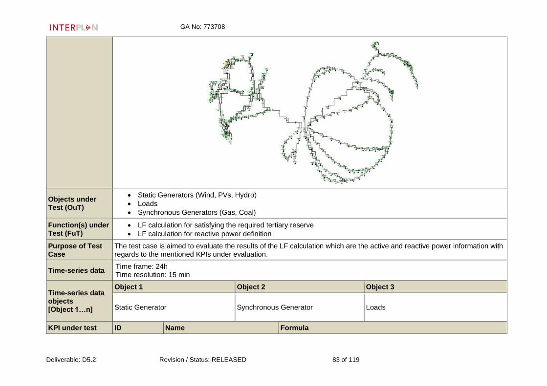
GA No: 773708
Deliverable: D5.2 Revision / Status: RELEASED 83 of 119
Objects under Test (OuT)
• Static Generators (Wind, PVs, Hydro)
• Loads
• Synchronous Generators (Gas, Coal)
Function(s) under Test (FuT)
• LF calculation for satisfying the required tertiary reserve
• LF calculation for reactive power definition
Purpose of Test Case
The test case is aimed to evaluate the results of the LF calculation which are the active and reactive power information with regards to the mentioned KPIs under evaluation.
Time-series data Time frame: 24h Time resolution: 15 min
Time-series data objects [Object 1…n]
Object 1 Object 2 Object 3
Static Generator Synchronous Generator Loads
KPI under test ID Name Formula

GA No: 773708
Deliverable: D5.2 Revision / Status: RELEASED 84 of 119
1 Level of losses in transmission and distribution networks
𝑃𝑒𝑟𝑐𝑒𝑛𝑡𝑎𝑔𝑒 𝑜𝑓 𝑙𝑜𝑠𝑠𝑒𝑠
= 𝐴𝑚𝑜𝑢𝑛𝑡 𝑜𝑓 𝑖𝑛𝑗𝑒𝑐𝑡𝑒𝑑 𝑒𝑛𝑒𝑟𝑔𝑦 − 𝑎𝑚𝑜𝑢𝑛𝑡 𝑜𝑓 𝑒𝑛𝑒𝑟𝑔𝑦 𝑑𝑒𝑙𝑖𝑣𝑒𝑟𝑒𝑑 𝑡𝑜 𝑡ℎ𝑒 𝑐𝑢𝑠𝑡𝑜𝑚𝑒𝑟𝑠
𝐴𝑚𝑜𝑢𝑛𝑡 𝑜𝑓 𝑖𝑛𝑗𝑒𝑐𝑡𝑒𝑑 𝑒𝑛𝑒𝑟𝑔𝑦× 100
10 Voltage Quality
According to the defined EN 50160 Standards and VDE-AR-N 4120
bus bar voltage magnitudes must comply with following allowed range
of variation.
• LV, MV: (±10% of nominal voltage)
• HV & EHV: (±4-7% of nominal voltage)
Voltage deviation indices can be defined to find the frequency or
duration that the bus bar voltages violate the allowed voltage range.
• Number of voltage excursions exceeded n minutes per year
• Percentage of time that the transmission voltage exceeds the
permissible limits
13
Mean quadratic deviations from voltage and reactive power targets at each connection point between TSO and DSO grids
Let C be the set of connection points between TSOs and DSOs. Let qc,target (t) [kVar] be the target value for reactive power transmission from DSO to TSO at connection point c and time t, as e.g. calculated by grid operation planning. Let qc(t) be the reactive power actually provided from DSO to TSO at connection point c and time t. Then the KPI related to reactive power at time t is defined as: 1
|𝐶|∑(𝑞𝑐,𝑡𝑎𝑟𝑔𝑒𝑡(𝑡) − 𝑞𝑐(𝑡))
2
𝑐∈𝐶
The KPI related to voltage is defined as follows. Let uc,target [V] be the nominal value for the line-to-line voltage at connection point c, calculated as mean over all phases. Let uc(t) be the actual line-to-line voltage mean over all phases. Then, the KPI at time t is: 1
|𝐶|∑(𝑢𝑐,𝑡𝑎𝑟𝑔𝑒𝑡 − 𝑢𝑐(𝑡))
2
𝑐∈𝐶
14 Level of DG / DRES utilization for ancillary services
𝑈𝐴𝑆% = 𝐸𝐴𝑆
𝐸𝑡𝑜𝑡𝑎𝑙 ∗ 100 [%]
𝐸𝐴𝑆 − 𝑡ℎ𝑒 𝑒𝑛𝑒𝑟𝑔𝑦 𝑢𝑠𝑒𝑑 𝑓𝑜𝑟 𝑎𝑛𝑐𝑖𝑙𝑙𝑎𝑟𝑦 𝑠𝑒𝑟𝑣𝑖𝑐𝑒𝑠 [𝑀𝑊ℎ]

GA No: 773708
Deliverable: D5.2 Revision / Status: RELEASED 85 of 119
𝐸𝑡𝑜𝑡𝑎𝑙 − 𝑡ℎ𝑒 𝑡𝑜𝑡𝑎𝑙 𝑒𝑛𝑒𝑟𝑔𝑦 𝑝𝑟𝑜𝑑𝑢𝑐𝑒𝑑 [𝑀𝑊ℎ]
16 Transformer loading 𝐿𝑜𝑎𝑑𝑖𝑛𝑔% = 𝑃𝑜𝑤𝑒𝑟 𝑎𝑡 𝑡𝑟𝑎𝑛𝑠𝑓𝑜𝑟𝑚𝑒𝑟 𝑝𝑟𝑖𝑚𝑎𝑟𝑦 𝑤𝑖𝑛𝑑𝑖𝑛𝑔
𝑇𝑟𝑎𝑛𝑠𝑓𝑜𝑟𝑚𝑒𝑟 𝑛𝑜𝑚𝑖𝑛𝑎𝑙 𝑝𝑜𝑤𝑒𝑟 ∗ 100
23 Mean quadratic deviations from active power targets at TSO/DSO connection points
Let C be the set of connection points between TSOs and DSOs. Let pc,target (t) [kW] be the target value for active power transmission from DSO to TSO at connection point c and time t, as e.g. calculated by grid operation planning. Let pc(t) be the active power actually provided from DSO to TSO at connection point c and time t. Then the KPI related to active power at time t is defined as: 1
|𝐶|∑(𝑝𝑐,𝑡𝑎𝑟𝑔𝑒𝑡(𝑡) − 𝑝𝑐(𝑡))
2
𝑐∈𝐶
27 Share of RES
𝑅𝐸𝑆% = 𝑃𝑅𝐸𝑆
𝑃𝑡𝑜𝑡𝑎𝑙 ∗ 100 [%]
𝑃𝑅𝐸𝑆 − 𝐴𝑐𝑡𝑖𝑣𝑒 𝑝𝑜𝑤𝑒𝑟 𝑝𝑟𝑜𝑣𝑖𝑑𝑒𝑑 𝑏𝑦 𝑅𝐸𝑆 𝑎𝑡 𝑎 𝑔𝑖𝑣𝑒𝑛 𝑡𝑖𝑚𝑒 𝑠𝑡𝑒𝑝 [𝑀𝑊] 𝑃𝑡𝑜𝑡𝑎𝑙 − 𝑇𝑜𝑡𝑎𝑙 𝑎𝑐𝑡𝑖𝑣𝑒 𝑝𝑜𝑤𝑒𝑟 𝑝𝑟𝑜𝑣𝑖𝑑𝑒𝑑 𝑏𝑦 𝑅𝐸𝑆 𝑎𝑛𝑑 𝑛𝑜𝑛− 𝑅𝐸𝑆 𝑔𝑒𝑛𝑒𝑟𝑎𝑡𝑜𝑟𝑠 𝑎𝑡 𝑎 𝑔𝑖𝑣𝑒𝑛 𝑡𝑖𝑚𝑒 𝑠𝑡𝑒𝑝𝑡𝑜𝑡𝑎𝑙 𝑖𝑛𝑠𝑡𝑎𝑙𝑙𝑒𝑑 𝑐𝑎𝑝𝑎𝑐𝑖𝑡𝑦 [
Variability attributes (test factors)
No parameters are varied.
Simulation environment
DIgSILENT PowerFactory
Simulation type Semi-dynamic
Output parameters
Active and reactive power set points, power losses, share of RES in generation (generation costs)....
Initial system state
Steady state
Evolution of system state and test signals
No event is considered

GA No: 773708
Deliverable: D5.2 Revision / Status: RELEASED 86 of 119
Other parameters Grid model data (e.g transmission line parameters)
Temporal resolution
15 minutes within 24 hours in total
Source of uncertainty
Time series data (Availability of demand response and renewable energy resources)
Suspension criteria / Stopping criteria
LF does not converge
5.4.3 Test case results
ID/Title Simulation results for BSC4 by using the SimBench-based grid model
KPI evaluation
ID Name Value
1 Level of losses in transmission and distribution networks
Presented in figure for KPI 1 in the following.
10 Voltage quality Presented in figure for KPI 10 in the following.
13
Mean quadratic deviations from voltage and reactive power targets at each connection point between TSO and DSO grids
Presented in figure for KPI 13 in the following.
14 Level of DG / DRES utilization for ancillary services
This KPI is zero for this BSC, since this BSC does not assume utilisation of DG/DRES for ancillary services as no controls are active.
16 Transformer loading Presented in figure for KPI 16 in the following.
23 Mean quadratic deviations from active power targets at TSO/DSO connection
Presented in figure for KPI 23 in the following.

GA No: 773708
Deliverable: D5.2 Revision / Status: RELEASED 87 of 119
points
27 Share of RES Presented in figure for KPI 27 in the following.
Results
The percentage of power losses at TSO level is shown in the figure above for all time steps. The power losses rate is varying between 1% to 2%. The KPI is calculated only for transmission level as the base showcase simulation is limited to this voltage level.

GA No: 773708
Deliverable: D5.2 Revision / Status: RELEASED 88 of 119
This figure above depicts the voltage magnitude for all 20 buses in TSO level at each time step. Each colour represents the nodes and shows that all voltage values are between 0.96 and 1.04 p.u.. According to EN 50160 and VDE-AR-N 4120 Standards, the voltage tolerance in HV should be maximum ±5% of the nominal voltage.
This figure above depicts the voltage and reactive power deviation. The target value for voltage is set 1 p.u.; for reactive

GA No: 773708
Deliverable: D5.2 Revision / Status: RELEASED 89 of 119
power, it is set to zero. Moreover, for both formulations C, set of connection point, is 1 and the square root is calculated for both. The figure shows that reactive power and voltage deviation from target values in the connection point are near constant at off peak hours. At peak hours, the voltage has lower deviation from 1 p.u., while the reactive power deviation from zero is higher. The reason of choosing zero for reactive power target is to decrease the interaction among TSO and DSO.
The figure above shows the loading percentage of the transformers connecting TSO and DSO levels. There are three connection points and each of them has two transformers. The loading percentages of both transformers in every connection point are the same. Obviously, the loading percentages during demand peak hours are higher than at the rest of the day.

GA No: 773708
Deliverable: D5.2 Revision / Status: RELEASED 90 of 119
This figure above depicts the mean quadratic deviations from active power targets at TSO/DSO connection points. The target value for active power at all TSO - DSO connection points is set to zero, in order to evaluate how independent the DSO network can be operated from the TSO network. Moreover, in the calculation of KPI, C, as connection point set in the formula, set to 1 and the square root was added to the formula, eventually. As expected, at peak hours, the deviation from the active power target is higher because more active power is exchanged between DSO and TSO at those hours.

GA No: 773708
Deliverable: D5.2 Revision / Status: RELEASED 91 of 119
The figure above presents the share of RES in active power generation in percentage. As a part of the grid model under investigation represents an external unknown grid, this part of the grid has been excluded for calculation of the KPI value.
Network operation criticalities found
In the simulation of this base showcase, the following operation issues have been found:
• Power losses at TSO level for some time steps are considerable with regards to the average power losses at transmission level in Germany according to [6].
• There may be a possibility to decrease transformer loading at some time steps.
• There may be a possibility to increase the share of RES at some time steps.
Possible solutions identified
Optimising the reactive and active power distribution among the resources with the aim of minimising the power losses as well as increasing the share of RES in balancing and ancillary service. This approach meant for day-ahead operation planning of the network will be implemented in the control functions related to SC4. A comparison will be made by considering the aforementioned KPIs in order to evaluate the effectiveness of the control functions embedded in SC4.

GA No: 773708
Deliverable: D5.2 Revision / Status: RELEASED 92 of 119
5.5 Optimal energy interruption management - BSC5 5.5.1 Base showcase properties
ID BSC_5
Associated Showcase
SC_5 Optimal energy interruption management
Base showcase description
The base show case prepares the network for a set of credible contingencies and configures inputs for the showcase control function. The control function then minimizes the energy interruption in the presence of a contingency event by re-scheduling the generators and controlling interruptible loads. The base showcase activates the contingency and analyse the KPIs that are then later compared with the outputs of the showcase control function.
Sub base use cases involved - associated use cases
7.1 - Optimal generation scheduling and sizing of DER for energy interruption management
For a given time step, an LF is performed and contingencies that can occur in transmission or distribution system are enlisted. They are either specified by a TSO/DSO or can be listed based on peak loaded lines/transformers or the terminals having peak voltage levels. One of the contingencies is activated and LF is performed. The KPIs of the showcase are calculated. Afterwards, sensitivity analysis is performed towards the heavily loaded line/transformer or bus in the post-contingency scenario. This information is used to prioritize resources that can effectively meet the demand and to prevent the network constraint violation.
Sequence diagram

GA No: 773708
Deliverable: D5.2 Revision / Status: RELEASED 93 of 119
Timing diagram
Sequence of actions
Step Event name Event description
Information Exchange (if any)
Information producer (actor/tool)
Information receiver (actor/tool)
Information Exchanged IDs
1
Grid information, load and generation profile are incorporated in the network
Scenario preparation necessary to collect all information per each resource in the grid
TSO/DSO Grid simulation tool (Grid, loads, generators objects)
IEX_1
2 Location and profile for RES
Scenario preparation necessary to collect all information per RES added to the grid
TSO/DSO Grid simulation tool (generator objects)
IEX_2
3 Load shedding flexibility
Scenario preparation. Here, the loads interruption flexibility is defined in terms of the level and related
TSO/DSO Grid simulation tool (load objects)
IEX_3
tA
Cycle m
tA : Start of scenario, preparation of network
tB : Start of use-case scenario selection, preparation of the network
tC : Load flow initialization, constraint definition and optimization
tB

GA No: 773708
Deliverable: D5.2 Revision / Status: RELEASED 94 of 119
cost
4 LF and sensitivity analysis
Performing LF and sensitivity analysis to identify grid operation limits violations
Grid simulation tool Grid simulation tool IEX_4
5 Hosting capacity calculation
This function calculates the maximum level of RES that can be integrated at the given locations in the grid connected to each node
Grid simulation tool Grid simulation tool (Nominal power of the generator objects)
IEX_5
6 Definition of list of credible contingencies
Use the results of steps 4 and 5 to define a list of credible contingencies
Grid simulation tool Grid simulation tool IEX_6
7 Contingency activation LF analysis
Activation of the first contingency from the contingencies list and run an LF analysis
Grid simulation tool Grid simulation tool IEX_7
8 Defining constraints for control algorithm
Defining constraints for the control algorithm
Grid simulation tool TSO/DSO IEX_8
Domain under Investigation (DuI):
Transmission and distribution grid
Scenario under Investigation
INTERPLAN_2: Small and Local
GA No: 773708
Deliverable: D5.2 Revision / Status: RELEASED 95 of 119
(SuI)
5.5.2 Test case properties
ID/Title Implementation of the base showcase a synthetic grid
Narrative of the Test Case
The objective of this test case is to perform optimal energy interruption planning in order to minimize the total cost of ene rgy interruption for the synthetic grid. The control variables are the active and reactive power set-points of the generators and the curtailable loads. The test case formulates an instance of the base showcase that identifies the list of credible contingencies.
System under Test (SuT)
The system under test is the synthetic grid model. This grid model has 10 detailed feeder models and number of equivalent feeder models representing typical urban and rural distribution networks. The grid model consists of HV, MV and LV parts.
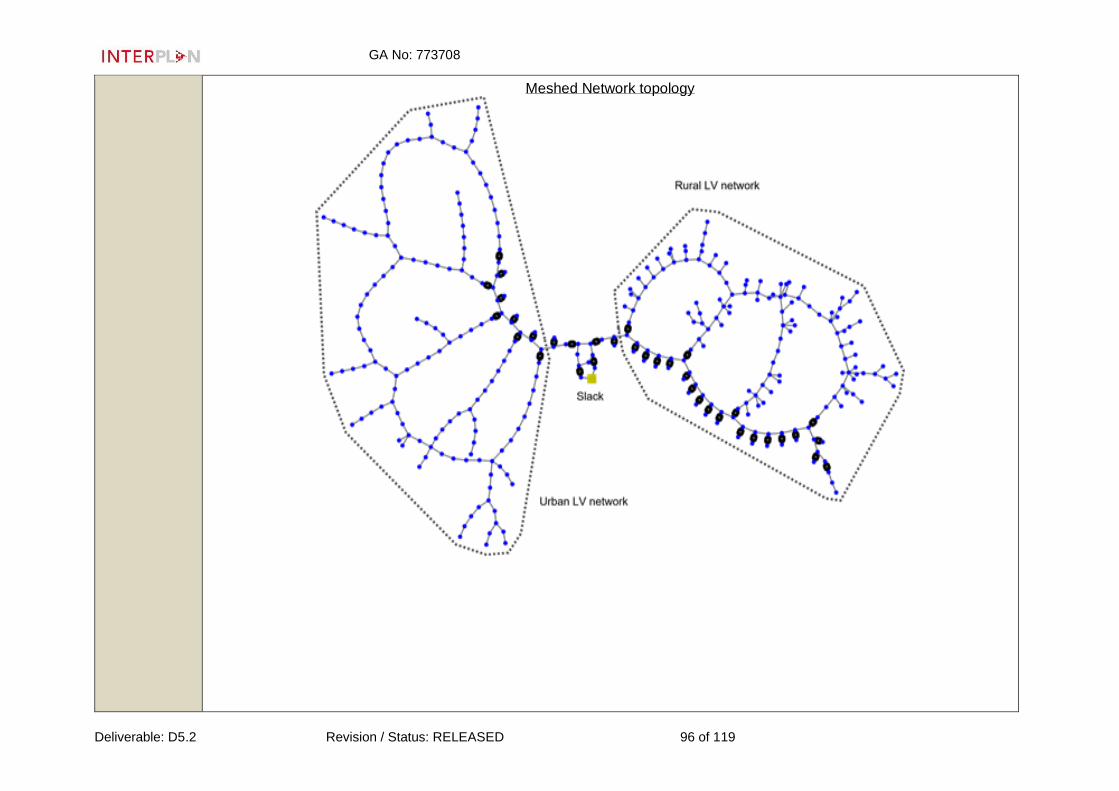
GA No: 773708
Deliverable: D5.2 Revision / Status: RELEASED 96 of 119
Meshed Network topology

GA No: 773708
Deliverable: D5.2 Revision / Status: RELEASED 97 of 119
Radial Network Topology
Objects under Test (OuT)
The PowerFactory objects that are members of the contingency list are sequentially made “out of service” to simulate the contingency event. The loads objects have the information about the extent and the cost of load shedding while the generator objects have the dispatch capability defined.
Function(s) under Test (FuT)
• LF
• LF sensitivities
• Reliability analysis
Purpose of Test Case
The purpose of the test case is to validate that all the necessary data for the showcase is available and the control process can be performed
Time-series data
Load, PV, generators profiles are available for one day to one year. Time resolution is 15 minutes.

GA No: 773708
Deliverable: D5.2 Revision / Status: RELEASED 98 of 119
Time-series data objects [Object 1…n]
Object 1 Object 2 Object 3
Loads profiles PVs active power profiles Generators dispatch profiles
Other input data
The cost of energy interruption as the energy tariff and the reliability data of the lines, buses, transformers, generators.
KPI under test
ID Name Formula
3 SAIDI (System Average Interruption Duration Index )
𝑆𝐴𝐼𝐷𝐼
=𝑠𝑢𝑚 𝑜𝑓 𝑎𝑙𝑙 𝑐𝑢𝑠𝑡𝑜𝑚𝑒𝑟 𝑖𝑛𝑡𝑒𝑟𝑟𝑢𝑝𝑡𝑖𝑜𝑛 𝑑𝑢𝑟𝑎𝑡𝑖𝑜𝑠
𝑡𝑜𝑡𝑎𝑙 𝑛𝑢𝑚𝑏𝑒𝑟 𝑜𝑓 𝑐𝑢𝑠𝑡𝑜𝑚𝑒𝑟𝑠 𝑠𝑒𝑟𝑣𝑒𝑑
7 Power losses
𝑃𝑙𝑜𝑠𝑠𝑒𝑠 = ∑ |𝐼|𝑖2 ∗ 𝑟𝑖 [𝑘𝑊]
𝑁𝑙𝑖𝑛𝑒
𝑖
𝐼𝑖 − 𝑚𝑎𝑔𝑛𝑖𝑡𝑢𝑑𝑒 𝑜𝑓 𝑐𝑢𝑟𝑟𝑒𝑛𝑡 𝑓𝑙𝑜𝑤 𝑖𝑛 𝑙𝑖𝑛𝑒 𝑖 [𝐴] 𝑟𝑖 − 𝑟𝑒𝑠𝑖𝑠𝑡𝑎𝑛𝑐𝑒 𝑜𝑓 𝑙𝑖𝑛𝑒 𝑖 [𝛺]
8 AENS & ENS (Average Energy not Supplied & Energy not Supplied)
𝐴𝐸𝑁𝑆 = 𝐸𝑁𝑆 ∑ 𝐶𝑖⁄
𝐸𝑁𝑆 = ∑ 𝐿𝑃𝐸𝑁𝑆𝑖
𝐿𝑃𝐸𝑁𝑆𝑖 : Load Point i Energy Not Supplied 𝐶𝑖 : : Customer i
𝐴𝐶𝐼𝑇 : Average Customer Interruption Time
9 IEAR( Interrupted Energy Assessment Rate)
𝐼𝐸𝐴𝑅 =𝐸𝐼𝐶
𝐸𝑁𝑆 in $ / kWh
𝐸𝐼𝐶: Expected Interruption Cost, in units of
[M$/y], is the total expected interruption cost
𝐸𝑁𝑆: Energy Not Supplied, in units of [MWh/a], is the total amount of energy on

GA No: 773708
Deliverable: D5.2 Revision / Status: RELEASED 99 of 119
average not delivered to the system loads
18 SAIFI(System Average Interruption Frequency
Index)
𝑆𝐴𝐼𝐹𝐼
= 𝑡𝑜𝑡𝑎𝑙 𝑛𝑢𝑚𝑏𝑒𝑟 𝑜𝑓 𝑐𝑢𝑠𝑡𝑜𝑚𝑒𝑟 𝑖𝑛𝑡𝑒𝑟𝑟𝑢𝑝𝑡𝑖𝑜𝑛𝑠
𝑡𝑜𝑡𝑎𝑙 𝑛𝑢𝑚𝑏𝑒𝑟 𝑜𝑓 𝑐𝑢𝑠𝑡𝑜𝑚𝑒𝑟𝑠 𝑠𝑒𝑟𝑣𝑒𝑑
Variability attributes (test factors)
The objects that are part of the contingency list are made out of service (binary status).
Quality attributes
The generator active and reactive power limits and dis-patchable loads flexibility potential sets the boundary conditions of control. The network voltage and loading constraints are to be strictly kept under the limits.
Simulation environment
DIgSILENT PowerFactory and Python
Simulation type
Steady state LF
Output parameters
Credible contingencies list, preliminary results of energy not supplied, energy not supplied costs, System Average Interruption Frequency Index (SAIFI), System Average Interruption Duration Index (SAIDI), Interrupted Energy Assessment Rate (IEAR) and other KPIs values.
Test design parameters
Due to changing state of the LV grids (renewable energy connections, e-charging stations and distributed storage) and consequential impact on the MV grids, it is essential to investigate the significant potential hazards in grid operations that cannot be avoided using protection schemes. Currently, there is non-availability of such tools that can be used dynamically to plan in such situations.
Initial system state
Steady state
Evolution of system state and test signals
Making the object from the contingency list out of service
Other parameters
Topological model of the grid
Storage of data
PowerFactory (*.pfd), excel (*.xlsx, *.csv)

GA No: 773708
Deliverable: D5.2 Revision / Status: RELEASED 100 of 119
Temporal resolution
15 minutes within 24 hours. However, also longer period (one year) could be considered based on the data availability
Source of uncertainty
The uncertainty in the grid model and of load profiles is not taken in to account.
Suspension criteria / Stopping criteria
• LF does not converge
• Operational constraints are violated
• Reliability analysis cannot be performed
• Insufficient data regarding load shedding
5.5.3 Test case results
ID/Title Simulation results for BSC5 by using a synthetic grid model
KPI evaluation
ID Name Value
18
System Average Interruption Frequency Index (SAIFI)
See figures below for KPI 18
3 System Average Interruption Duration Index (SAIDI)
See figures below for KPI 3
8
Average Energy not Supplied and Energy not Supplied (ENS, AENS)
See figures below for KPI 8
9 Interrupted Energy Assessment Rate (IEAR)
See figures below for KPI 9
7 Power losses See figures below for KPI 7

GA No: 773708
Deliverable: D5.2 Revision / Status: RELEASED 101 of 119
Results
This figure represents the values of KPI 18 SAIFI for a meshed network for different contingencies
This figure represents the cumulative distribution function (cdf) of KPI 18 SAIFI for a meshed network for different contingencies

GA No: 773708
Deliverable: D5.2 Revision / Status: RELEASED 102 of 119
This figure represents the values of KPI 18 SAIFI for a radial network for different contingencies
This figure represents the cdf of KPI 18 SAIFI for a radial network for different contingencies

GA No: 773708
Deliverable: D5.2 Revision / Status: RELEASED 103 of 119
Results
This figure represents the values of KPI 3 SAIDI for a meshed network for different contingencies
This figure represents the cdf of KPI 3 SAIDI for a meshed network for different contingencies

GA No: 773708
Deliverable: D5.2 Revision / Status: RELEASED 104 of 119
This figure represents the values of KPI 3 SAIDI for a radial network for different contingencies
This figure represents the cdf of KPI 3 SAIDI for a radial network for different contingencies
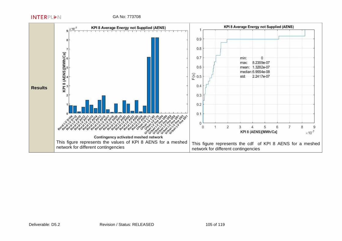
GA No: 773708
Deliverable: D5.2 Revision / Status: RELEASED 105 of 119
Results
This figure represents the values of KPI 8 AENS for a meshed network for different contingencies
This figure represents the cdf of KPI 8 AENS for a meshed network for different contingencies

GA No: 773708
Deliverable: D5.2 Revision / Status: RELEASED 106 of 119
This figure represents the values of KPI 8 AENS for a radial network for different contingencies
This figure represents the cdf of KPI 8 AENS for a radial network for different contingencies

GA No: 773708
Deliverable: D5.2 Revision / Status: RELEASED 107 of 119
This figure represents the values of KPI 9 IEAR for a meshed network for different contingencies
This figure represents the cdf of KPI 9IEAR for a meshed network for different contingencies

GA No: 773708
Deliverable: D5.2 Revision / Status: RELEASED 108 of 119
This figure represents the values of KPI 9 IEAR for a radial network for different contingencies
This figure represents the cdf of KPI 9 IEAR for a radial network for different contingencies

GA No: 773708
Deliverable: D5.2 Revision / Status: RELEASED 109 of 119
Results
This figure represents the values of KPI 7 Power losses for a meshed network for different contingencies
This figure represents the cdf of KPI 7 Power losses for a meshed network for different contingencies

GA No: 773708
Deliverable: D5.2 Revision / Status: RELEASED 110 of 119
This figure represents the values of KPI 7 Power losses for a radial network for different contingencies
This figure represents the cdf of KPI 7 Power losses for a radial network for different contingencies
Network operation criticalities found
In the simulation results, the following operation criticalities are found:
• Overloaded lines on MV and LV level;
• Voltage violations (over and under voltages) on MV and LV level
Possible solutions identified
This criticalities were foreseen as list of credible contingencies that can occur and lead to energy interruptions and loss of service with related costs. To solve these problems and minimize the interrupted energy and their related costs and in meanwhile keep the operational condition within the limitations, the possible solutions could be:
• Optimal active power re-dispatching among TSO and DSO assets so that the over voltage constraints problem for most nodes can be solved to be within the limits during the contingency if it occurs.
• In mean while PV curtailment is active, automatic controlled PV units can be used for solving over voltage problems.
• Optimal load shedding so that the under voltage constraints problem for most nodes can be solved to be within the limits during
GA No: 773708
Deliverable: D5.2 Revision / Status: RELEASED 111 of 119
the contingency if it occurs.
• The target is to minimize the load shedding and its related costs while satisfying the network constraints.
These proposed solutions will be implemented in the control functions related to SC5 “Optimal energy interruption management”. A comparison will be made considering the KPIs identified in the BSC 5 to keep line and transformer loadings within certain l imits <=80% and the voltage within the defined limits according to the defined European EN 50160 Standards, which specify that the bus bar voltage magnitudes must comply with following allowed range of variation.
• LV, MV: (±10% of nominal voltage)

GA No: 773708
Deliverable: D5.2 Revision / Status: RELEASED 112 of 119
6. Summary and outlook
The deliverable provides the detailed description of the INTERPLAN Integrated Network Operation
Planning tool and presents the results of the dynamic and semi-dynamic simulations for the five
INTERPLAN base showcases.
The INTERPLAN tool is defined as a methodology consisting of a set of tools (grid equivalents,
control functions) for the operation planning of the Pan-European network by addressing a significant
number of system operation planning challenges of the current and the future 2030+ EU power grid,
from the perspective of the transmission system, the distribution system, and with a particular focus
on the transmission-distribution interface.
The tool consists of three main stages (1. Simulation functionalities, KPIs and scenario selection, 2.
Grid model selection/preparation, 3. Simulation & Evaluation), each of them consisting of a number
of steps to be performed by the user (a TSO or a DSO) for the operation planning of the network
under consideration. In developing such a tool, the following goals have been considered:
• Make the tool as responsive as possible to meet the critical needs of grid operators in
addressing a wide range of operation challenges covering all network levels and for
increasing TSO-DSO cooperation for operation planning purposes.
• Make the tool flexible enough to be adapted to the current and future grid scenarios.
• Make the tool flexible enough in the application of grid equivalents when they are needed for
studying specific operation challenges covering multiple voltage levels.
• Make the tool flexible enough in the integration of the various sub-tools and components
developed or to be developed in INTERPLAN (planning criteria, KPIs, scenarios, grid
equivalenting, use cases and showcases with the related control functions).
• Make the tool feasible for its application in real practice, by also identifying how the tool could
look like in the future. In this sense, from the practical point of view, the INTERPLAN tool will
be a Python-based toolbox interfacing with PowerFactory (under the simulation phase in
stage 3), consisting of a library of grid equivalents and control functions for use cases and
showcases for addressing the related operational challenges under the selected scenario
and operation planning criteria.
The main strengthen points of the tool proposed are:
• It allows facing with the operation planning of the Pan-European network through an
integrated approach, by offering the possibility to investigate all network voltage levels for
operational planning purposes, while also integrating the actions made by different
stakeholders such as TSOs and DSOs, which are considered as the primary users for the
tool.
• With the current network operation planning approaches, it is not possible to consider all
existing networks (including full models) in an integrated planning tool due to computational
limitations, lack of detailed models, etc. Through the intrinsic grid equivalenting methodology
and the related grid equivalents library, the tool allows simplifying certain parts of a grid while
keeping the relevant characteristics.
• Through the control functions embedded within INTERPLAN use cases and showcases, the
tool allows addressing a number of operational challenges of the current and future 2030+
power networks from the perspective of both TSOs and DSOs.
The “proof-of-concept” of INTERPLAN tool will be verified within the INTERPLAN control system
logics development, through one of the INTERPLAN use cases or showcases selected by the
consortium also based on the consultation with external relevant stakeholders.
Another key item addressed in this deliverable refers to the simulations of basic grid equivalents for
the five INTERPLAN base showcases associated to the following showcases:

GA No: 773708
Deliverable: D5.2 Revision / Status: RELEASED 113 of 119
• Low inertia systems;
• Effective DER operation planning through active and reactive power control;
• TSO-DSO power flow optimization;
• Active and reactive power flow optimization at transmission and distribution networks;
• Optimal energy interruption management
A base showcase is defined as a combination of sub base use case(s) with no planning criteria and
no controllers for emerging technologies, such as RES, DG, demand response or storages. For each
showcase, there is a relevant base showcase with the same grid model, scenario, KPIs, simulation
environment, simulation type and time-series data. The simulation of base showcases is a key
aspect to evaluate effectiveness, reliability and robustness of the control functions proposed in the
associated showcases, which will be developed, implemented and simulated in Task 5.3. The key
findings of base showcases simulations are summarized below:
• In BSC1 simulation, it is found that several system security criteria are not met. In particular,
the criteria related to stability and security of operation returned a few cases in which they
are not met. Since the results are highly reliant on the operating point of the power system,
a measure to improve situation is to change the operating point of particular devices in
particular moments during the analysed (planned) operation period. However, this should be
considered as last resort not only because it collides with market solution of the LF, but also
because there are better means to do it. The synthetic inertia concept will be applied to
available resources and a new methodology for frequency control will be used. Thus by
including novel dynamic control methods, re-dispatching and/or curtailment costs can be
avoided.
• In BSC2 simulation focusing on transmission grid level, congestion events are identified and
power losses are found considerable for some time steps as compared to the average power
losses at transmission level for the geographic area under consideration. The possible
solutions identified consist of the optimal active power re-dispatching among both TSO and
DSO assets such that to obtain a loading value less than 90% for all lines in the grid model
under consideration. This re-dispatching function can involve both resources connected at
transmission level and flexibility resources connected at distribution level. Moreover,
considering the optimal active power set-points re-dispatched to solve congestion events, an
optimal power flow can be performed to minimize the power losses in a way that optimum
reactive power set points and voltage set points are acquired.
• In BSC3 simulation, similar to BSC2, a similar problem of considerable power losses is found
at transmission level, and the identified solution consists of an optimal power flow calculation
which minimizes the power losses considering the role of DGs and RES in ancillary services
provision.
• The problem of considerable power losses at transmission level is found also in BSC4
simulation. Another key result found in BSC4 simulation is that the share of RES could be
increased at some time steps, and the transformer loading could decrease at some time
steps. Optimising the reactive and active power distribution among the resources with the
aim of minimising the power losses as well as increasing the share of RES in balancing and
ancillary service represents the solution identified to address these issues.
• In BSC5 simulation, overloaded lines are found at MV and LV levels and some voltage
violations are also found on both MV and LV levels. This criticalities are foreseen as list of
credible contingencies that can occur and lead to energy interruptions and loss of service
with related costs. To solve these problems and minimize the interrupted energy and their
related costs and in meanwhile keep the operational condition within the limitations, the
possible solutions could be:
o Optimal active power re-dispatching among TSO and DSO assets so that the over
voltage constraints problem for most nodes can be solved to be within the limits

GA No: 773708
Deliverable: D5.2 Revision / Status: RELEASED 114 of 119
during the contingency if it occurs.
o In meanwhile PV curtailment is active (automatic controlled PV units) can be used for
solving over voltage problems.
o Optimal load shedding so that the under voltage constraints problem for most nodes
can be solved to be within the limits during the contingency if it occurs.
o The target is to minimize the load shedding and its related costs while satisfying the
network constraints.
These potential solutions identified for INTERPLAN base showcases related to the day-ahead
operation planning will be implemented in the control functions embedded within the associated
showcases. A comparison will be also made through the KPIs with the aim to show the effectiveness
of the control functions in solving the operation issues identified.

GA No: 773708
Deliverable: D5.2 Revision / Status: RELEASED 115 of 119
7. References
[1] INTERPLAN, "Deliverable D5.1 INTERPLAN showcases", (Public report), December 2018.
[2] INTERPLAN, "Deliverable D3.2 INTERPLAN scenarios and use cases", (Public report), October 2018.
[3] INTERPLAN, "Deliverable D4.2 Approach for generating grid equivalents for different use cases (first version)", (Public report), September 2019.
[4] INTERPLAN, "Deliverable D6.1 INTERPLAN scenarios which will be validated in the simulation", (Public report), May 2019.
[5] INTERPLAN, "Deliverable D4.1 Method for clustering distributions grid", (Public report), May 2019.
[6] Council of European Energy Regulators asbl, “CEER Report on Power Losses”, October 2017,
available online “https://www.ceer.eu/documents/104400/-/-/09ecee88-e877-3305-6767-
e75404637087#targetText=Overall%2C%20in%202015%20we%20note,%25%20and%2010.
44%25%20across%20Europe.”

GA No: 773708
Deliverable: D5.2 Revision / Status: RELEASED 116 of 119
8. Annex 8.1 List of Figures Figure 1: INTERPLAN concept ......................................................................................................... 10 Figure 2: INTERPLAN tool overview ................................................................................................ 14 Figure 3: Stage 1 of INTERPLAN tool .............................................................................................. 17 Figure 4: Stage 2 of INTERPLAN tool .............................................................................................. 31 Figure 5: Stage 3 of INTERPLAN tool .............................................................................................. 38
8.2 List of Tables Table 1: Individual planning criteria vs applicable INTERPLAN use cases..................................... 17 Table 2: Groups of planning criteria vs applicable INTERPLAN showcases .................................. 18 Table 3: Sub-groups of planning criteria vs applicable INTERPLAN showcases ........................... 19 Table 4: Key performance indicators vs planning criteria ................................................................ 20 Table 5: Possible combinations allowed under stage 1 in case of selection of one planning criterion
.................................................................................................................................................... 22 Table 6: Possible combinations allowed under stage 1 in case of selection of a group of planning
criteria ......................................................................................................................................... 25 Table 7: Possible combinations allowed under stage 1 in case of selection of a sub-group of planning
criteria ......................................................................................................................................... 28 Table 8: Grid equivalenting information related to INTERPLAN use cases for enabled selections 33 Table 9: Grid equivalenting information related to INTERPLAN showcases for enabled selections
.................................................................................................................................................... 35 8.3 Glossary of terms and definitions 8.3.1 Definition of project general terms
Term Definition
Use Case The specification of a set of actions performed by a system, which yields an observable result that is, typically, of value for one or more actors or other stakeholders of the system.
Sub Use Case
Description of a specific situation a use case is applied to. A Sub Use Case is always attributed to one (main) use case, but one use-case may have multiple sub use cases which detail the main use case in at least one aspect.
Base showcase
Presentation of base use case(s) with no planning criteria and no controllers for emerging technologies, such as RES, DG, demand response or storages in the frame of chosen scenario, simulation type, test model, and time-series data. The base showcase allows to analyze the operation challenges of the related use case(s) and improvements achieved through the application of planning criteria with related implementation of controllers in the associated showcase.
Showcase Presentation of use case(s) in the frame of chosen scenario, simulation type, test model, time-series data and planning criteria
Scenario
Definition of a future situation applying to a well-defined time (most often year). A scenario can be fictional or predicted from the present situation. In INTERPLAN, scenarios describe the future situation of the European electric network, typically including grid topology, generation mix, loads and diffusion of EV, RES and storages.
Dynamic Simulation A simulation experiment which considers the time dependent behaviour of a physical system, looking at events occurring in real-time operation,

GA No: 773708
Deliverable: D5.2 Revision / Status: RELEASED 117 of 119
with a frequency of occurrence of less than one second of real time. The simulation may run faster or slower than real time, and may, despite the fast event frequency, span a total time interval of several hours real-time.
Semi-Dynamic Simulation (also: Quasi-Dynamic Simulation)
A medium- to long-term simulation experiment based on steady-state analysis, considering the state of a physical system at discrete steps of real time through user-defined time step sizes. The real time between the steps is at least one minute.
Grid Cluster A group of grids and parts of grids with similar characteristics
Grid Equivalent
A simplified network model, which approximately behaves like an associated complex physical network or a group of physical networks. The grid equivalent thus is a representation of the physical network(s), which is typically used for a simulation experiment.
Control function
A set point definition, which is determined based on the goals of each use case. A control function defines the set points of specific elements (e.g. OLTC, DGs, RESs) or some programs (e.g. demand response) calculated by an operation objective in the network..
Interface
A means of transmitting information between two or more controllers or actors. It usually includes a specification about which information is to be transmitted, how this information is represented by data elements, and defines a physical means for transmission of those data elements.
Cluster Controller A controller having the aggregated behavior of individual controller characteristic in a larger grid.
Interface Controller
A controller, which is intended to be installed in a specific "home" cluster, and uses information received through an interface from at least one other cluster data source outside the home cluster. This data source could e.g. be another cluster, but also e.g. an external weather forecast provider using an interface
Local Controller
A controller which is associated with a single specific generator, load or grid asset and which operation does not rely on remotely received information originating from any remote source. i.e. the operation only relies on information available within the local area network of the local controller’s installation site.
Co-simulation
A simulation which consists of different parts that form a coupled problem and are modelled and simulated in a distributed manner (cp. Wikipedia). The parts are called "Co-simulation subsystems" and are exchanging data during the simulation. Different models and simulation means can be used in different subsystems. The Co-simulation (in the ideal case) is carried out by running the subsystems, which were individually tested and validated beforehand, in a black-box manner. In INTERPLAN, the data exchange between subsystems is done by the OpSim platform.
Co-simulation subsystem / Co-simulation subcomponents
A part of a Co-simulation which is developed, modelled and validated individually, while at the same time able to be integrated into the Co-simulation platform. In INTERPLAN, a subsystem might represent e.g. a DSO or TSO operation centre, a controller, or even the real physical network model.
Data model
An abstract model that represents a real-world entity, and defines, organizes and standardizes the description of the data elements related with that entity. Since real-world entities are typically consisting of other entities (e.g. an electric grid consists of lines, transformers etc.), a data model typically is hierarchically structured and also allows to define interrelations between entities.

GA No: 773708
Deliverable: D5.2 Revision / Status: RELEASED 118 of 119
V2G and G2V
Vehicle-to-grid (V2G) describes a system in which plug-in electric vehicles communicate with the power grid to sell demand response
services by either returning electricity to the grid or by throttling their charging rate. When an EV is being charged, it’s called G2V (Grid to Vehicle).
Allocation
With reference to the grid operation planning phase, it is the process deciding, which are the most suitable resources to commit and dispatch among n operating resources for a specific objective and under specific constraints.
Placement and sizing
With reference to the grid planning, it is the process deciding the most proper location (bus) and the size of a resource (active power) for a specific objective and under specific constraints.
Energy Not Supplied Energy Not Supplied is defined as the amount of energy that would have been supplied to the customer if there had been no interruption.
Energy spillage Energy spillage is the production (from Solar and Wind) that is unable to be accommodated due to demand being lower than production.
8.3.2 Definition of actors
Term Definition
TSO -
Transmission
System
Operator
Natural or legal person responsible for operating, ensuring the maintenance
of the transmission system and, if necessary, developing the transmission
system in a given area and, where applicable, its interconnections with other
systems, and for ensuring the long-term ability of the system to meet
reasonable demands for the transmission of electricity. The term
‘transmission’ means the transport of electricity on the extra high-voltage and
high-voltage interconnected system with a view to its delivery to final
customers or to distributors, but does not include supply.
DSO -
Distribution
System
Operator
A natural or legal person responsible for operating, ensuring the maintenance
of and, if necessary, developing the distribution system in a given area and,
where applicable, its interconnections with other systems and for ensuring
the long-term ability of the system to meet reasonable demands for the
distribution of electricity. The term ‘distribution’ means the transport of
electricity on high-voltage, medium-voltage and low-voltage distribution
systems with a view to its delivery to customers, but does not include supply.
ESCO
Electricity supply company (sometimes also: Electricity service company).
General term for a company which supplies end users with electric energy.
An ESCO may offer additional services, e.g. electricity generation, metering
or supply with non-electric energy.
Prosumer
Active energy consumer who consumes and produces electricity. Various
types of prosumers exist: residential prosumers who produce electricity at
home - mainly through rooftop PV, citizen-led energy cooperatives,
commercial prosumers whose main business activity is not electricity
production, and public institutions.
Generator A device which produces electricity.
Load A device which consumes electricity.
Producer A natural or legal person generating electricity.
Consumer A natural or legal person consuming electricity.
Distributed A source or sink of electric power that is located on the distribution system,

GA No: 773708
Deliverable: D5.2 Revision / Status: RELEASED 119 of 119
Energy
Resource (DER)
any subsystem thereof, or behind a customer meter. DER may include
distributed generation, electric storage, electric vehicles and demand
response.
Aggregator
Company who grouping distinct agents in a power system (i.e. consumers,
producers, prosumers, or any mix thereof) to act as a single entity when
engaging in power system markets (both wholesale and retail) or selling
services to the system operator(s).
Distributed
generation (DG)
unit
Any source of electric power of limited capacity, directly connected to the
power system distribution network. DG can be powered by photovoltaic
system, micro-turbines, combustion engines, fuel cells, wind turbines,
geothermal, etc.
Flexible Loads
A load which consumption can be influenced in terms of power, time, or total
energy consumed while still serving its intended purpose. The influence may
be exerted by manual means (e.g. switching the load on or off at arbitrary
times) or automatic means (e.g. external control signal).