WOBURNCHILDHOOD LEUKEMIA

FOLLOW-UP STUDYVolume IAnalyses

FINAL REPORT

July 1997

Massachusetts Department of Public HealthBureau of Environmental Health Assessment

ACKNOWLEDGEMENT

This study could not have been completed without the support and cooperation of the Woburncommunity. In particular we would like to acknowledge Gretchen Latowsky and the membersof the community organization For A Cleaner Environment (FACE), former Superintendent ofSchools Paul J. Andrews, former Woburn High School Principal James J. Foley, AssistantSuperintendent of Schools Louise M. Nolan, and members of the Woburn Advisory Panel fortheir assistance and support. We would also like to thank Dr. Peter Murphy for his work in thedevelopment of the Woburn Water Distribution Model, the Citizens Advisory Council for theirconstructive comments during the development of our research protocol, and the study subjectfamilies for their willingness to be interviewed as part of this important research effort.

EXECUTIVE SUMMARY

Woburn, Massachusetts, is a community of approximately 35,000 people, located13 miles northwest of Boston. It has an extensive industrial history spanning over 130years which included greenhouse operation, leather manufacturing and chemicalmanufacturing. Products manufactured included arsenic compounds used in pesticides,textiles, paper, TNT, and animal glues. The deposition of hazardous material and wasteproducts from these industries has been a long-standing point of environmental concernfor citizens and government officials.

In 1979, environmental concerns were brought to the forefront of public attentionwhen excavation of a former industrial site unearthed significant amounts of industrialwaste that proved to be contaminated with high levels of lead, arsenic, and heavymetals. It was subsequently learned that two municipal drinking water wells which hadbeen installed near this site were contaminated with trichlorethylene (TCE), perchloro-ethylene, chloroform and other organic compounds. These wells had supplied publicwater primarily to the eastern portion of Woburn between 1964 and 1979.

Woburn residents were concerned regarding health effects that may have resultedfrom consumption of the contaminated water. These concerns were heightened when itwas learned that between January 1969 and December 1979, twelve cases of childhoodleukemia had been diagnosed in Woburn, six of these cases resided in a six-block areawhich was served directly by the contaminated wells. Identification of these casesprompted the Massachusetts Department of Public Health (MDPH) and the Centers forDisease Control (CDC) to begin a formal investigation of the health status of Woburnresidents.

Results of a case-control investigation conducted by MDPH were published inJanuary 1981. The investigation concluded: (1) the incidence of childhood leukemiawas significantly elevated in Wobum (12 observed cases vs. 5.3 expected cases between1969 and 1979); (2) the majority of the excess cases were males; and (3) six of the caseswere diagnosed while residing in a single census tract in Woburn. At the time, the casesin this census tract represented half the identified childhood leukemias, a numberdisproportionate to the geographic distribution of the population in the community. In1984, the MDPH released a summary report which identified an additional seven casesdiagnosed through 1983 and demonstrated a continued excess in the incidence ofchildhood leukemia (19 observed cases vs. 6. 1 expected).

By the middle of 1986, a total of 21 childhood leukemia cases had beendiagnosed in Woburn. Cases diagnosed after 1979 had birth residences, which weremore evenly distributed throughout Woburn than the original 12 cases. As a result of

the continued elevated incidence and the change in the geographic distribution of thecases, MDPH conducted the Childhood Leukemia Follow-Up Study.

Study Design

The study is a matched case-control design with two controls selected for eachcase. All cases were children 19 years of age or younger and diagnosed with leukemiabetween 1969 and 1989 while residents of Woburn. Controls were selected randomlyfrom Woburn school records and matched to cases based on date of birth (plus or minus3 months), sex and race. Controls must have been Wobum residents at the time ofdiagnosis of the matched case. Residential, occupational and health history data werecollected during interview for the etiologic period for each case and its matchedcontrols. The etiologic period is defined as the period of time from two years beforeconception to the case’s leukemia diagnosis and is sub-divided for analysis into the timesegments two years before conception to conception, during pregnancy, and from birthto case diagnosis.

Results

Univariate AnalysesDetailed analyses of data collected at interview revealed five variables for which

10 or more total positive responses were identified and that demonstrated odds ratiosgreater than or equal to 1.50 in relation to the childhood leukemia incidence.

Maternal alcohol consumption during pregnancy (O.R- = 1. 50, C.I. = 0. 54, 4.20);diagnosis of a paternal grandfather with cancer (O.R- = 2.01, C.I. = 0.73, 5.58); havinga fatherwho worked for industries considered high risk for occupational exposures (O.R- =2.50, C.I. = 0.78, 8.30); and the subject’s consumption of public water as their primarybeverage (O.R- = 3.03,C.I. = 0.82, 11.28) were all variables which showed non-significant but positive associations with childhood leukemia incidence. A statisticallysignificant association was identified between developing childhood leukemia and beingbreast-fed as a child (O.R- = 10. 17, C.I. = 1.22, 84.58).

Multivariate Analyses and Exposure to Wells G and H

Multivariate analyses of the relationship between childhood leukemia andexposure to water from Wells G and H revealed that although five variables discussedabove showed elevated odds ratios as univariates in relation to the leukemia, they didnot significantly affect odds ratios specific to water exposure. Adjusted odds ratioswere calculated controlling for socioeconomic status, maternal smoking duringpregnancy, maternal age at birth of the child, and maternal alcohol consumption during

pregnancy. Of these variables, only maternal alcohol consumption during pregnancydemonstrated a slightly elevated odds ratio in univariate analyses. The literaturesuggests, however, that these variables are suspected to be associated with leukemiaincidence or adverse reproductive outcomes and were, therefore, kept in the model aspart of the primary analysis.

Adjusted odds ratios describing the effects of Wells G and H water on leukemiaincidence showed a non-significant elevation for the overall etiologic period (O.R- =2.39, C.I. = 0.54, 10.59) and each time period subcategory. The strongest relationshipbetween exposure and leukemia among time period subcategories is during pregnancy(O.R- = 8.33, C.I. = 0.73, 94.67), the second is in the two years before conception (O.R-= 2.61, C.I. = 0.47, 14.37) and the weakest is in the time period between the birth of thecase and the diagnosis of leukemia (O.R- = 1.18, C.I. = 0.28, 5.05).

Sub-stratification of the pregnancy time period to assess specific effects of waterexposure by trimester revealed high correlation coefficients between trimester exposurevalues. Independent effects of water exposure by trimester on leukemia incidencecould, therefore, not be distinguished with confidence.

Analyses to assess potential dose response relationships were completed using atrichotomous parameterization of the actual study subject exposure values by timeperiod. Results demonstrated elevated odds ratios between dose categories for thepreconception and pregnancy periods. A significant trend across exposure categorieswas also identified for the period during pregnancy (P < 0.05) suggesting a dose-response relationship for subjects whose mothers drank Wells G and H water duringpregnancy. Tests for trend for the etiologic period overall and for each of the other timeperiod subcategories were not significant (P > 0.05).

Discussion and Conclusions

This finding suggests that the relative risk of developing childhood leukemia wasgreater for those children whose mothers were likely to have consumed water fromWells G and H during pregnancy this association showed a significantly positiverelationship to the amount of water households received. Further research in otherpopulations is necessary to definitively address this trend and examine potentialembryologic windows of increased vulnerability to leukemogens. In contrast, thereappeared to be no association between the development of childhood leukemia andconsumption of water from Wells G and H by the children prior to their diagnosis.

Few positive associations were identified between childhood leukemia incidenceand residential parental occupation, and medical history related risk factor information

collecting during interview. A statistically significant relationship was identifiedbetween breast feeding and childhood leukemia, although a mechanism for thisrelationship is unclear.

The literature demonstrates that certain chemical exposures have been associatedwith health effects in both children and adults. TCE, one chemical detected in the wellwater, is known to have weak hematologic effects in mammals but no effect on humansin studies thus far, although effects on the developing human fetus are unclear. Thenature and extent of historical contamination of Wells G and H is not known. However,in our study, it seems the exposure, whether multichemical or specific in nature, mayhave had an effect on blood-forming organs during fetal development, but not duringchildhood.

The small number of study subjects lead to imprecise estimates of risk. As aresult, the exact magnitude of the association between exposure to water from Wells Gand H and risk of childhood leukemia cannot be stated. Results, however, demonstrateconsistency in the direction of an association, suggest a dose-response relationship anddemonstrate a decrease in effect after the elimination of the potential for exposure. Weconclude that the incidence of childhood leukemia in Wobum between 1969 and 1989 isassociated with mothers' potential for exposure to contaminated water from Wells G andH, particularly for exposure during pregnancy.

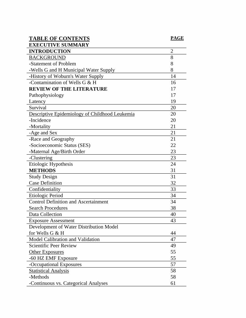
TABLE OF CONTENTS PAGE

EXECUTIVE SUMMARYINTRODUCTION 2BACKGROUND 8-Statement of Problem 8-Wells G and H Municipal Water Supply 8-History of Woburn's Water Supply 14-Contamination of Wells G & H 16REVIEW OF THE LITERATURE 17Pathophysiology 17Latency 19Survival 20Descriptive Epidemiology of Childhood Leukemia 20-Incidence 20-Mortality 21-Age and Sex 21-Race and Geography 21-Socioeconomic Status (SES) 22-Maternal Age/Birth Order 23-Clustering 23Etiologic Hypothesis 24METHODS 31Study Design 31Case Definition 32Confidentiality 33Etiologic Period 34Control Definition and Ascertainment 34Search Procedures 38Data Collection 40Exposure Assessment 43Development of Water Distribution Modelfor Wells G & H 44Model Calibration and Validation 47Scientific Peer Review 49Other Exposures 55-60 HZ EMF Exposure 55-Occupational Exposures 57Statistical Analysis 58-Methods 58-Continuous vs. Categorical Analyses 61

-Controlling For Confounding 61RESULTS 63Participation 63Description of Cases 65Exposure to Wells G and H Water 66Analysis of other Possible Risk Factors 74-Residential History 75-Occupational History 75-Study Subject Medical History 79-Maternal Pregnancy History 80-60 Hz EMF 84-Other Risk Factors 85DISCUSSION 86Normalization of Exposure Scores 92Other Risk Factors 9360 Hz Electric Magnetic Fields 97Comparison with the Harvard Study Findings 98Plausibility of Results 101Confounding and Bias 103CONCLUSIONS AND RECOMMENDATIONS 104

INTRODUCTION

The purpose of this investigation, as proposed in November 1987, was to provide further

insight into the causes of childhood leukemia among persons nineteen years of age or younger

who were diagnosed with leukemia between January 1, 1969 and August 31, 1989 and were

residents of Woburn at the time of their diagnosis. No new childhood leukemia cases were

diagnosed, however, until early in 1994. This work serves to supplement previous efforts of the

Massachusetts Department of Public Health (MDPH) (Parker and Rosen, 1981) (Friede, 1984)

which confirmed the increased incidence of childhood leukemia in Woburn.

The objective of this study was to re-analyze the original data set by obtaining more

complete information for the twelve childhood leukemia cases included in the 1981 investigation

and to expand the study to include the additional 9 cases diagnosed as of August, 1989. This

investigation has utilized more refined scientific methods for exposure assessment made

available during the Woburn Environment and Birth Study and information regarding potential

causes of cancer not available at the time of the original MDPH study. It directly evaluates the

relationship between exposure to water from Wells G and H and childhood leukemia incidence

and how other potential risk factors may have contributed to the increased incidence.

BACKGROUND

Statement of the Problem

The City of Woburn, Massachusetts is located approximately 13 miles northwest of

Boston. It has been an industrial community for over 130 years hosting a variety of industries

including greenhouses, leather manufacturers and chemical manufacturers producing products

such as arsenic compounds for insect control, textiles, paper, TNT, and animal glues.

Complaints by citizens regarding water quality and ambient air odors date back for over 100

years.

In the spring and summer of 1979, attention was drawn to environmental hazards in

Woburn when excavation in an 800 acre industrial area of the city revealed substantial hazardous

wastes. Abandoned lagoons severely contaminated with lead, arsenic, heavy metals and buried

animal hides were unearthed on the site commonly known as Industri-Plex. The unearthed hides

released high levels of hydrogen sulfide and methane gas that spread the familiar Woburn odor

to surrounding communities. The issue drew public attention when toxic waste disposal at the

town dump was revealed and when municipal drinking water testing indicated the presence of

contamination in two wells. City Wells G and H were found to be contaminated with

trichloroethylene (TCE), perchloroethylene, chloroform, and other organic compounds. The

wells were first used in 1964 but were shut down by the Department of Environmental Quality

Engineering (DEQE, now the Department of Environmental Protection (DEP)) in 1979 when

the contamination was discovered. They had been used to supplement Woburn’s public water

supply particularly in East Woburn.

Woburn residents, having become concerned regarding possible ill health effects the

contamination may have caused, became alarmed when they identified twelve cases of childhood

leukemia in the community that had been diagnosed between January 1969 and December 1979.

The Centers for Disease Control (CDC) also received a report from a Boston pediatric

hematologist stating that he had identified six of these cases in a six block area of Woburn.

These events prompted the Massachusetts Department of Public Health (MDPH) and the CDC

to begin a formal investigation of the health status of Woburn residents.

A report was published by MDPH in January 1981 entitled "Woburn Cancer Incidence

and Environmental Hazards, 1969-1978". It outlined the results of the MDPH/CDC

case-control study which concluded: 1) the incidence of childhood leukemia was significantly

elevated in Woburn (12 observed cases vs. 5.3 expected cases); 2) the majority of the excess

cases were males, and 3) six of the cases were diagnosed while residing in a single census tract

in Woburn. At the time, the cases in this census tract represented half the childhood leukemias,

a number disproportionate to the geographic distribution of the population in the community.

In November of 1981, MDPH released a second report entitled "Cancer Mortality in

Woburn, A Three Decade Study (1949-1978)." This report reviewed trends in leukemia

mortality before, during, and after the use of the contaminated wells. It concluded that

childhood leukemia mortality was not elevated during the period between 1949 and 1958 but

began to rise between 1959 and 1963. No unusual geographic distribution of childhood

leukemia mortality occurred during the period from 1949 to 1968.

In February of 1984, Harvard researchers published the results of a study they conducted

in Woburn during 1982 (Lagakos, 1986) to address the childhood leukemia concerns and to

examine other health outcomes as well. Harvard researchers were interested in determining if

elevations in childhood leukemia incidence rates remained elevated beyond 1979, after the

original MDPH report. The researchers also wished to further investigate the relationship

between the incidence of childhood leukemia and the availability of water from Wells G and H.

Their analysis included 15 childhood leukemia cases who were born during the period

1960 to 1972 and were residents of Woburn at the time of diagnosis. The 15 cases included 11

of the 12 original MDPH cases. One MDPH case born before 1960 was excluded, and four

other cases diagnosed in Woburn between 1980 and 1982 were added. They determined that

Woburn's childhood leukemia rate continued to be elevated through 1982.

The Harvard researchers administered a telephone survey questionnaire to 3257

households in Woburn between April and September 1982. The questionnaire was designed to

yield additional data for the determination of an association between the contaminated water and

childhood leukemia. A water distribution simulation model prepared by the DEQE, now the

DEP, was used to provide information concerning the amount of mixing of public water from

different sources and its distribution to homes throughout Woburn. The DEQE study estimated

on a monthly basis which of five identified zones of graduated exposure received none, some, or

all of their water from Wells G and H.

Researchers then estimated the percentage of each household's annual water supply that

arose from Wells G and H. The data was used to assign to each subject a cumulative exposure

score beginning with the annual exposure score corresponding to the mother's residence in the

year the pregnancy ended. The child's individual score would be the sum of the scores for each

year of their Woburn residence within the study period. If a child changed residences, the child's

score for that year was arbitrarily defined as the score corresponding to the former residence.

(Lagakos, 1986).

The Harvard study determined positive associations between water use from the

contaminated wells and the risk of childhood leukemia, prenatal death (post 1970),

lung/respiratory disorders, kidney/urinary disorders, eye/ear birth defects, and "environmental"

birth defects- an arbitrarily constructed grouping of those birth defects that reportedly have been

linked in the scientific literature with external environmental factors such as chemicals,

pesticides, radiation, or trace elements in water. The study recommended that town and state

health departments consider initiating a long-term health surveillance system for the monitoring

of childhood and reproductive disorders.

In 1984, as a result of the availability of cancer incidence data from the newly created

Massachusetts Cancer Registry, MDPH released updated information concerning Woburn

childhood leukemia incidence (Memorandum from A. Friede to J. Cutler, 1984). They

confirmed seven new cases since the release of their January 1981 study that included three new

cases since the Harvard Study was completed. The total number of childhood leukemia cases

was then nineteen.

Geographically, the seven new cases were distributed more randomly throughout the city

than the original twelve and were not limited to the areas supplied by the contaminated wells.

Analysis of the entire group of cases diagnosed through 1983 revealed a continued leukemia

excess than at the time of the original investigation. Three census tracts now showed a

significant elevation in incidence as opposed to only one census tract originally.

As a result of this continued trend, MDPH with financial support from the CDC drew

together an advisory panel comprised of experts in the field of epidemiology, prenatal

epidemiology, toxicology, environmental engineering, genetics, medicine, statistics, sociology,

and virology. The Woburn Advisory Panel reviewed the studies and background information to

date and provided recommendations (Woburn Advisory Panel, 1985) to MDPH. Among its

recommendations the expert panel suggested "a closer investigation of incident cases of

childhood leukemia and their families in the continuing search for etiologic clues."

Between 1986 and August 1, 1989, two additional cases were diagnosed for a total of

twenty-one childhood leukemias identified as having been diagnosed in children up to nineteen

years of age between 1969 and 1989. The cases belonged to three of the four histopathological

types of leukemia. Seventeen cases have been identified as acute lymphocytic leukemia (ALL),

3 cases as acute myelocytic leukemia (AML) and 1 case as chronic myelocytic leukemia (CML).

None of the children were reported as having the fourth major histopathologic type, chronic

lymphocytic leukemia (CLL).

Leukemia cases diagnosed after 1979 had birth residences that appeared to be more

evenly distributed throughout Woburn than previous cases, suggesting that factors other than

geographic area of residence may be related to leukemia incidence. In order to examine the

leukemia incidence more closely, MDPH decided to expand their 1981 analysis by re-examining

the twelve cases they studied originally and adding the more recently identified cases to their

analysis. The Woburn Childhood Leukemia Follow-Up Study included the twenty-one cases of

childhood leukemia reported to the MDPH from hospitals or the Massachusetts Cancer Registry

as having been diagnosed between January 1, 1969 and August 31, 1989.

The Woburn Advisory Panel also suggested the establishment of a surveillance system to

monitor the frequency of selected reproductive outcomes in Woburn as an indicator of potential

health effects the environmental exposures may be having on the community. In response, the

Massachusetts Department of Public Health and the U.S. Centers for Disease Control and

Prevention formed a cooperative agreement in order to complete the Woburn Environment and

Birth Study (WEBS) (1994). The WEBS study found that, in general, birth defect rates in

Woburn were no different from the rates for the twelve communities surrounding Woburn for

the study period.

History of Wells G and H Municipal Water Supply

History of Woburn's Water Supply

The City of Woburn has had a long history of problems with water quality, as well as an

inadequate volume of water. Documented water supply problems date back to the late 1800's,

persisting through May 1979. Although May 1979 coincides with the date that the

Massachusetts Department of Environmental Protection (MA DEP) advised that the water from

Woburn's Wells G and H should not be used for public water supply purposes (McCall, 1979),

the history of water quality problems more directly relates to Woburn's various industrial

activities and the pollution of aquifers that underlie the City, as well as pollution of the Aberjona

River running through Woburn.

During the period 1871-1911, the prime sources of pollution of the Woburn sections of

the Aberjona River and its tributaries were the tanneries, leather-related industries, and chemical

industries. From 1911 through 1956, tannery pollution and chemical wastes continued as the

major sources of surface and groundwater contamination, impacting upon City sewerage

systems. The period 1956 through 1984 was marked by the development and discovery of

additional water pollution sources by a variety of firms conducting other forms of industrial

activity, (Tarr, 1987).

In 1955 the City of Woburn contracted with Whitman and Howard, Inc. to conduct a

study of the Woburn water system and recommend improvements (Tarr, 1987). Contained in

that report was a reference to the use of the Aberjona River Valley (Aberjona Aquifer) as a

source of public water supply. This report states, "the Aberjona River Valley still has a potential

for groundwater supply for certain industrial uses, but the groundwater of this valley are, in

general, too polluted to be used for public water supply," (Whitman and Howard, 1958).

Despite this warning, increased demands on the town's water supply by the mid-1960s led to the

digging of test wells at various sites in the Aberjona Aquifer, including Wells 15 and 16, later to

become Wells G and H, respectively (Tarr, 1987).

Wells G and H were put into service during the 1960's as supplementary water sources.

Well G began pumping in October of 1964 and Well H began pumping in the first half of 1967

(Tarr, 1987). They were in service for 2995.5 days, representing a little more than half of the

total days of their period of operation. The Wells drew water from the Aberjona River Aquifer

and provided approximately 24% of the City's water supply (Special Legislation Commission on

Water Supply, 1986). Woburn's other municipal supply wells drew water from the Horn Pond

Aquifer.

Throughout the Wells G and H period of operation, there are repeated references (1964

through 1977) to the poor quality of the water pumped from the Wells, including reports of

elevated levels of nitrates, ammonia, nitrogen, chlorides, sulfates, sodium, manganese, iron, and

a reference as early as 1964 to the "presence of some organic materials" (Tarr, 1987). Other

complaints by residents included bad taste, odors, color and staining of plumbing fixtures and

laundry. Some residents reported that they could tell when the Wells were in service because of

the marked change in water quality. MA DPH, in 1975, advised the City to seek an alternative

water supply due to the poor aesthetic water quality.

The discovery of nearby toxic wastes in 1979 led to the testing of Wells G and H for

chemical contaminants by the MA DEP. Trichloroethylene (267 ppb) and tetrachloroethylene

(21 ppb) were found to exceed drinking water guidelines. Low levels of chloroform, methyl

chloroform, trichlorotrifluoroethane, 1,2-dichloroethylene and inorganic arsenic were also

detected. As a result of these tests, Woburn's Wells G and H were closed in May, 1979.

Today, the Massachusetts Water Resource Authority provides 40% of Woburn's water

and the remaining 60% of Woburn's water supply is drawn from the Horn Pond Valley from

gravel wells on the westerly and southerly shores of the pond. Woburn's Horn Pond water

supply system is possibly the oldest municipal system in Massachusetts (verbal communication,

City of Woburn Pumping Station personnel, 1992).

Contamination of Wells G & H

Documents developed by the United States Environmental Protection Agency (US

EPA), the MA DEP, and their consultants provided information on groundwater contamination

and the industries that were responsible for contaminating Wells G and H. The MA DPH

conducted a Wells G and H Health Assessment in 1989, in collaboration with the Agency for

Toxic Substances and Disease Registry (ATSDR), to evaluate the public health implications

associated with the levels of contamination detected in Wells G and H, the contaminated

groundwater within the area of influence of Wells G and H, and the contaminants found in

various media in and around what has come to be known as the Wells G and H National Priority

List (NPL) site (Wells G and H, 1989).

Five properties within the Wells G and H site have been determined to contain soil

contamination and contributed to the contamination of groundwater in the vicinity of Wells G

and H. These properties ranged in distance from 200 to 2300 feet to the wells.

It was not possible to establish when chemical contaminants first reached the Wells, nor

the degree to which concentrations of various chemicals may have varied over time. It was

possible, however, to examine the known hydrology of the area and contaminated groundwater

plumes and it was deemed plausible that contaminated groundwater reached Wells G and H

prior to 1979.

For the purposes of this study, it was assumed that the chemical substances determined

to be of concern to public health and detected in the groundwater at the five properties

presumed to be responsible for contaminating Wells G and H had, in fact, reached the wells

prior to 1979. These chemical substances include trichloroethylene, tetrachloroethylene, trans-

1-dichloroethylene, arsenic, lead, chlordane, 1,1,1-trichloroethylene, chloroform, methyl

chloroform, and vinyl chloride.

REVIEW OF THE LITERATURE

Pathophysiology

Leukemia literally means "white blood" -- a reference to the excessive numbers of

leukocytes (or white blood cells) in the peripheral blood of leukemics. The serious symptoms of

the disease, however, are caused by a lack of normally functioning cells and/or platelets; this

deficiency is brought about through proliferation of cells that resemble a stage in normal

blood-cell development but which are incapable of performing the functions of mature blood

cells [Miller et al., 1986; Clarkson, 1980] such as fighting off foreign invaders to the body by

attacking them (the function of some granulocytes and the "T" lymphocytes) or releasing

harmful substances (the function of some granulocytes and the "B" lymphocytes).

The transformation from normal precursor to leukemic cell can occur at various points

along the developmental pathways of the granulocytes and lymphocytes [Clarkson, 1980].

Conditions referred to as "acute" leukemias result from early transformations which leave cells

blocked at an immature stage. Different acute leukemias are distinguished by the type of

immature cell that is found in the peripheral circulation (where mature cells are needed). The

most common form of leukemia affecting children (80 percent of childhood cases [MacMahon,

1992a]) is acute lymphoblastic (or lymphocytic) leukemia (ALL), in which lymphoblasts fail to

develop into lymphocytes and accumulate. It is important to recognize that adult ALL and

childhood ALL may be distinct entities. Although Doll [1989] has stated that the distinction

between childhood and adult leukemia is not absolute, Schull, et al. [1988] considers differences

between childhood and adult cases in terms of cell types, chromosomal markers, and response to

therapy as indications of the involvement of different cellular and molecular events at different

ages. Even childhood ALL is heterogeneous in that any of three different types of lymphoblasts

may constitute the abnormal species in a particular case [Cresanta, 1992]. Accumulation of B

lymphoblasts (a feature of 90% of childhood ALL cases [Doll, 1989]) characterizes the disease

as it occurs in young children [Kaye et al., 1991]. T lymphoblasts, on the other hand,

accumulate in the blood of older childhood ALL victims [Kaye et al., 1991].

When myelocytes, which normally develop into granulocytes, are found in the peripheral

blood, the condition is referred to as acute myelocytic leukemia (AML). AML also occurs in

children; however, it is only about one-fifth as common as ALL in this period, occurring at a

rate of eight cases per million in infancy, as compared to 38 cases of ALL per million in children

under the age of five [Linet, 1985].

It is worthy of note that, if the leukemic transformation occurs in one or a few cells, as is

believed [Clarkson, 1980], the potential remains for the production of normal cells as well.

Eventually, though, the normal precursors to all blood cells are greatly reduced through an

inhibitory effect of the leukemic cells or their products [Clarkson, 1980; Linet, 1985; Miller et

al., 1986] such that the untreated patient is threatened by hemorrhage, infection, and inadequate

cellular nutrition [Miller et al., 1986].

The chronic leukemias are so called because the duration of these forms tends to be

longer, although remissions are achieved through medical treatment in all types of leukemia

[Smith, 1986; Clarkson, 1980]. Chronic lymphocytic leukemia (CLL) is unheard of in children

[Draper et al., 1993], and the rate of chronic myelogenous leukemia in children and young adults

is only two cases per 1,000,000 population [Linet, 1985]. Due to the rarity of chronic leukemia

in children, these forms will not be discussed.

Latency

As with other forms of cancer, latency is a feature of the natural history of leukemia.

"Latency" refers to the tendency for a disease to first become evident long after the underlying

malignant process has begun. "Induction period," a related term, is the time between first

exposure to the cause of interest (and, of course, there are likely to be multiple causes for any

case of cancer) and the start of the disease process. Neither latent periods (defined here as the

time between disease onset and detection) nor induction times can be measured; we must be

satisfied with knowing the length of the empirical induction time -- the time between the

occurrence of the exposure of interest and the detection of signs of disease.

Comparatively speaking, empirical induction times for leukemogenic agents are shorter

than those observed for other types of cancer [Land and Norman, 1978; Smith and Doll, 1978].

Leukemia occurred in survivors of atomic bomb blasts in Hiroshima and Nagasaki from two to

thirty years after exposure [Heath, 1982; Ohkita et al., 1978; Shore, 1989]. In this population,

some evidence has accrued of a negative relationship between amount of radiation and induction

time [Land and Norman, 1978]; generally speaking, though, shorter induction times were

observed for younger victims [Heath, 1982]. Children exposed in utero to diagnostic X-rays,

however, developed leukemia at between ten and 15 years of age [Stewart and Kneale, 1970].

Furthermore, recently completed cluster investigations demonstrated clustering of births for

older-diagnosed cases and clustering of residences occupied near the time of diagnosis for

younger diagnosed cases. These data tend to indicate that, even among children, younger age at

exposure may be associated with shorter latency.

Survival

It is important to recognize that, despite progress over the past ten to fifteen years in the

chemotherapeutic induction of remissions from leukemia [Miller et al., 1986; Clarkson, 1980], it

remains a very serious disease. Complete remission implies no leukemic cells in either the bone

marrow or peripheral blood [Miller et al., 1986], but relapses are common, such that the term

"complete remission" should not be confused with cure. Also, because acute leukemias are

generally fatal if untreated [Clarkson, 1980], therapeutic interventions tend to be aggressive and

involve hospitalizations and long-term administration of maximally tolerated doses of highly

toxic drugs [Miller et al., 1986]. With such treatment, 90 percent of the victims of pediatric

ALL (a disease that was almost universally fatal prior to 1965 [Pratt et al., 1988]) go into

complete remission, and today, 72 percent of this group achieves long-term leukemia-free

survival [American Cancer Society, 1993]. The five-year survival rate is much higher for ALL

than for AML, however [Page and Asire, 1985].

Descriptive Epidemiology of Childhood Leukemia

Incidence

Fewer than 10,000 cases of all types of cancer combined are diagnosed in American

children each year [Tarbell et al., 1986]; however, a large percentage of these are leukemias.

According to the American Cancer Society [1993], 2,600 children in the U.S. will have been

diagnosed with leukemia in 1993 and ALL, which occurs at an average annual rate of 32 cases

per million children under age 15 [Kaye et al., 1991], will be the specific diagnosis of 2,000 of

these.

Mortality

Mortality from childhood cancer in general has decreased steadily from 90 deaths per

million children in 1950 to 50 per million in 1978 [Li, 1982] to 40 per million in 1989 [American

Cancer Society, 1993].

Age and Sex

AML occurs at a constant low rate throughout early childhood, the annual incidence

rising sharply between the mid-teens and mid-twenties to about five to ten cases per million.

ALL shows a strikingly different pattern; peak incidence (around 40 cases per million [Linet,

1985]) occurs between ages one and four, and incidence decreases rapidly to a low of only

about one case per million population annually at around age 30 [Linet, 1985]. In childhood,

leukemia occurs only slightly more often in males versus females (sex ratio = 1.2 to 1.0 [Doll,

1989]), and the age patterns for the two sexes are similar [MacMahon, 1992a].

Race and Geography

Doll [1989] reports that, when certain outliners are excluded, the range in incidence of

all childhood cancers worldwide is quite narrow (31 to 49 cases per million population). The

notable exceptions are Africa, Fiji, and some parts of Asia, where incidence ranges between 10

and 20 cases per million. Black populations everywhere also exhibit low incidence; childhood

leukemia was found to be diagnosed only half as frequently in black children versus white

children by the Third National Cancer Survey [Li, 1982].

Interestingly, where incidence is low, the early childhood peak in ALL incidence is also

missing [Doll, 1989]. This difference could well be due to detection bias resulting from

decreased medical attention received by black children versus white children. Reports of low

leukemia incidence have been noted in parts of Africa with "good medical facilities and

well-trained hematologists," leading them to conclude that childhood leukemia actually occurs

less frequently in black populations versus white.

In a California study, Shaw et al. [1984] found a statistically significant association

between having a Spanish surname and leukemia registrations -- a finding that was unaffected by

restriction of analyses to residents of an area with complete reporting. The racial mixture of

controls was representative of the underlying population.

Socioeconomic Status (SES)

Results of some studies of childhood leukemia have suggested an association with high

socioeconomic status (SES) [Shaw et al., 1984, Ramot and Magrath, 1982; Van Steensel-Moll

et al., 1986; Lancet editors, 1990]. However, the link has recently been described as "modest"

[Alexander et al., 1990a] and "weak" [MacMahon, 1992a], and some researchers have failed to

find it at all [Shaw et al., 1984].

Knox et al. [1984] suggested that the leukemia-SES association reflects a greater

tendency of high-SES children versus low-SES children to survive the infectious diseases of

infancy and early childhood. The weakening or disappearance of the leukemia-SES association

with time might be explicable in these terms, considering the secular decrease in infant death

rates due to infection.

Maternal Age/Birth Order

Children with Down Syndrome have higher rates of leukemia than do unaffected

children. Since Down Syndrome is related to maternal age and is believed to result from genetic

changes occurring during egg-cell division, researchers have looked for evidence of a link

between advanced maternal age and childhood leukemia in the hope of identifying a similar

etiologic mechanism. The conflicting conclusions of the relevant research led Shaw et al. [1984]

to test this hypothesis in a case-control study. These authors interpreted their results negatively,

however. Cases were found to be 2.29 times as likely as controls to have been born to a woman

aged 40 or older. This difference was not statistically significant, but only 15 subjects altogether

had mothers in this age range. Kaye et al. [1991] found a similar (and significantly elevated)

odds ratio when they compared the leukemia risk of children born to mothers who were 35+

years old to that of those who were younger.

Researchers have also disagreed on the relationship between birth order and childhood

leukemia incidence, with some investigators reporting that firstborn children are at higher risk

[Van Steensel-Moll et al., 1986; Roman et al., 1993] while others have found higher risk

associated with later birth orders [Shaw et al., 1984]. An interesting new finding reported by

Kaye et al. [1991] concerns an association between leukemia risk and the number of years

between one's birth date and that of his/her next older sibling.

Clustering

No discussion of the epidemiology of childhood leukemia would be complete without

some exploration of its reputation as a disease that occurs in clusters. Most simply defined,

clustering is the close occurrence in time and space of different cases of a particular disease. If

the disease in question were infectious, we would refer to a cluster as an "epidemic." By

extension, we could say that a cluster is a non-infectious disease epidemic.

The significance that has been attached to clustering derives from its resemblance to a

feature of infectious-disease epidemiology, such that it has been taken by some as evidence that

childhood leukemia has an infectious cause. There are reasons to suspect an infectious etiology

for childhood leukemia, but it would be naive either to consider clustering as proof of an

infectious etiology or to interpret a lack of clustering as strong evidence against an infectious

origin. Any disease related to the environment would tend to cluster geographically, as would

any disease related to host factors if the affected hosts tended to cluster geographically.

Furthermore, although the absence of clustering could imply that disease occurrence is entirely

random, it could also mean that the risk factors are so evenly distributed across the population

that associations aren't discernible [Mathews, 1988].

Etiologic Hypotheses

In 1987, Sandler and Collman, referring to leukemia, wrote that "despite the extensive

literature devoted to the subject, little has been learned about risk factors for the disease."

These authors' conclusions related to adult leukemias, but Cartwright [1989] recently identified

risk factors for childhood ALL as "neonatal x-ray exposure, lack of vaccination and possible

unusual patterns of infection, chloramphenicol use and very little else." Actually, Sandler and

Collman [1987] question the connection between chloramphenicol use and leukemia, because

the case-report data have not been supported by experimental studies or by follow-up of patients

with chloramphenicol-induced bone marrow depression. Case reports have also implicated

phenylbutazone and cancer-chemotherapy drugs in non-lymphocytic leukemia causation.

Animal data have confirmed the association in the case of the anti-neoplastic [Sandler and

Collman, 1987]. Linet [1985] suggested further study for phenylbutazone, because, although

results of analytic studies had been negative, only two such investigations had been completed

by 1985.

Benzene

Both Linet [1985] and Austin et al. [1988] have reviewed the literature linking benzene

to leukemia. In introductory comments, the latter group of reviewers states that benzene is

widely considered to be a human leukemogen. Declining to consider the animal investigations

(though they do note that limited evidence of a carcinogenic effect has recently been

strengthened by further study), these authors identified fourteen epidemiologic investigations

concerning benzene and leukemia. Of the eleven papers published since 1977, five found

significant associations between benzene exposure or high benzene exposure and leukemia, and

in five, a positive but non-significant association was reported. Two of this latter group were

case-control studies based on very small numbers of cases (eleven and fifteen). The remaining

retrospective investigation was hospital based and relied on medical records to evaluate

exposure status (exposed versus not exposed). Only seven exposed patients were identified.

Other Solvents

Lowengart et al. [1987] performed a case-control study of children aged 10 years and

under in Los Angeles County to identify causes of acute leukemia. Analysis of 123 matched

pairs showed an increased risk of leukemia for children whose fathers were occupationally

exposed to certain chemicals after their birth. Results showed effects with chlorinated solvents

(OR = 3.0, p = 0.05), spray paint (OR = 2.0, p = 0.02), dyes (OR = 3.0, p = 0.05, and cutting oil

(OR = 1.7, p = 0.05). An elevated rate was also seen when a father was exposed to spray paint

during the mother's pregnancy. There was an increased risk for the child where parents used

pesticides in the home (or = 3.8, p = 0.004) or garden (OR = 6.5, p = 0.007).

Tobacco

Linet [1985] states that there is no evidence of a strong association between the

leukemias and tobacco use. She goes on to cite relative risks in the range of 1.5 from several

large prospective studies. A relative risk of 1.5 implies that the leukemia risk of smokers is one

and one half times that of nonsmokers. Relative risks under 2.0 are said to indicate weak

associations, and, unless demonstrated repeatedly in well designed studies, are considered

suspect, because they may be accounted for by uncontrolled "confounders." Confounders are

exposures or attributes which, through their association with both the exposure under

investigation and the outcome of interest, make it appear as though a causal relationship exists

between the supposed risk factor and the disease in question [Wald, 1988].

Sandler et al. (1993) reported in the results of a case-control study conducted with over

600 leukemia cases that smoking was associated with a modest increase in leukemia risk overall

(O.R. = 1.13, 95% C.I. = 0.89, 1.44). Researchers found, however, that among participants

aged 60 and older, smoking was associated with a twofold increase in the risk of acute myeloid

leukemia (AML) (O.R. = 1.96, 95% C.I. = 0.97, 11.9). No overall association between smoking

and leukemia among younger persons was identified. Among a subset of younger patients there

were associations between smoking and leukemia for patients with similar morphologic and

cytogenic features as the older cases.

Viruses

There are numerous reasons to believe that infectious agents cause leukemias. First and

foremost, perhaps, is the certainty of their role in animal leukemia [Heath, 1982]. Retroviruses,

which contain RNA as their genetic material [Davis et al., 1980], cause leukemia in cows, cats,

chickens, gibbons, birds, and primates. The viruses can be transmitted in various bodily fluids,

and leukemia follows infection by months or years [Linet, 1985]. The observation that leukemia

viruses cross species [Linet, 1985] barriers has perhaps fueled the search for evidence of

transmission of animal leukemia viruses to humans.

60 Hz EMF

In recent years a public health controversy has arisen concerning health effects and

exposure to extremely low frequency electric and magnetic fields (EMFs) produced by electrical

fixtures which produce, deliver, or use electricity. "EMF" is a general abbreviation for electric

and magnetic fields that are produced in all ranges of the electromagnetic spectrum. "EMF" has

commonly come into use in reference to extremely low frequency electromagnetic energy that is

sometimes abbreviated as ELF. This type of energy is produced by 60 Hertz (Hz) electric

power, the form of electricity carried by power lines and used in homes, offices, and factories.

Electric fields are produced by the presence of electric charges measured as voltage. Magnetic

fields are produced by the motion of electrical charges commonly referred to as current, and are

measured in units known as milligauss(Mg). The electric and magnetic fields produced by 60 Hz

electric power are referred to in this document as 60 Hz EMF.

At the present time it is difficult to say for sure if 60 Hz EMF is at all harmful to humans.

Some epidemiologic studies suggest that 60 Hz EMF either causes health effects directly or

promotes the development of health effects which were originally caused by some other adverse

environmental or non-environmental factor. Other studies suggest no such relationship. With

regard to cancer, even when an association has been demonstrated between some types of

cancer and 60 Hz EMF exposure, it has not been shown that 60 Hz EMF was the definitive

cause of the cancer. Laboratory studies have demonstrated that biological changes within cell

tissue cultures can be induced by 60 Hz fields, but these changes have not been linked to human

health effects.

The scientific community's current understanding of 60 Hz EMF exposure and its

possible relationship to health has focused on several different diseases. Although conclusions

regarding the amount of risk vary, most research indicates that children exposed to somewhat

higher levels of 60 Hz EMF in their home environment have at least a one and one half to two

times greater chance of being diagnosed with leukemia and cancers of the brain and nervous

system than children exposed long-term to 60 Hz EMF at lower levels (London, 1991) (Savitz,

et al., 1990).

In adults, a smaller but increased risk of leukemia and cancers of the brain and central

nervous system has been shown among workers in the electric power generating and electronics

manufacturing industries, occupations which are likely to have higher 60 Hz EMF exposure

(Folderus, 1992). Only a slight increased cancer risk has been observed among adults exposed

to elevated field strengths of 60 Hz EMF in residential settings.

Genetic Predisposition

Familial aggregation of leukemia -- a phenomenon which could result from inheritance or

from a shared environment -- is known [Linet, 1985; Heath, 1982; Sandler and Collman, 1987]

-- usually with a single cell type occurring in all affected family members. Investigators have

generally failed, however, to find blood-cell or other markers that typify affected members of

leukemia-prone families [Linet, 1985]. Heath [1982] reports that numerous surveys have

considered the question of familiarity without consistent evidence of more than faintly increased

risk to close relatives of leukemics. This author maintains that familial aggregation, if it does

exist, seems to involve mainly CLL, which does not occur in childhood. Few researchers have

attempted to describe variation in leukemia incidence or mortality with socioeconomic status,

and results have been equivocal -- with some studies failing to find any differences, some

showing a positive relationship, and some suggesting a negative association at least with some

subtypes [Linet, 1985]. The hypothesis has existed for some time, however, that the increases

noted above in worldwide incidence and mortality and other within-country trends are related to

improved living conditions -- an association which may be confounded by industrialization or

urbanization.

Parental Occupation

Considerable attention has also been given to the possible relationship between

childhood leukemia occurrence and parental occupational exposures. Although a better case

could perhaps be made for a link between maternal exposures (especially during pregnancy) and

childhood cancer, most studies of this subject have concerned paternal exposures -- probably

because of the historical predominance of men in the work force, and particularly in those jobs in

which chemical exposure would be likely. Savitz and Chen [1990] have noted that, for father's

occupation to be causally linked to childhood cancer, either the child would have to be exposed

directly to chemicals brought into the home, or the chemicals would have to alter the father's

germ cells.

In 1990, Savitz and Chen found 24 relevant studies to review. All had case-control

designs, and most relied on job titles recorded on birth certificates or reported at interview for

exposure assessment. Many job titles were found to be associated with childhood cancer

occurrence, but there were inconsistencies in the data, which Savitz and Chen thought might

have derived from inconsistency of design (e.g., some studies concentrated on particular cancer

types, subtypes, or age groups, while others considered childhood cancer or childhood leukemia

in the aggregate).

The reviewers seemed to be of the opinion that, because of weaknesses in the study

designs, particularly with respect to exposure assessment, the research thus far completed was

useful mainly as a screening mechanism and that in future studies further attention should be

paid to paternal paint exposure and paternal hydrocarbon exposure because of the relatively

strong and reproducible associations found between jobs that would afford these exposures and

childhood leukemia.

Radiation

Leukemia as a late effect of radiation exposure has been recognized since 1944 (a decade

after Marie Curie's death from radiation-induced leukemia [Lancet editors, 1984]), when March

reported that this disease was nine times more commonly recorded as a cause of death among

radiologists versus other physicians [Linos et al., 1980; Gee, 1987; Linet, 1985; Berry, 1987].

Today, cancer is well recognized as the principal health hazard associated with exposure to small

doses of ionizing radiation [Fry, 1981; Rossi, 1980; Rahn et al. 1984; Upton, 1982; Gofman,

1979], most of our understanding of the carcinogenic effects having been gleaned from studies

of survivors of the atomic-bomb detonations that ended World War II.

The low leukemia death rates found among those in utero ATB (20 cancer deaths per

million per rad [Mole, 1975]) can be contrasted with the elevated leukemia rates (240 per

million per rad [Mole, 1975]) associated with prenatal X-ray exposure in the Oxford Survey of

Childhood Cancers (OSCC) [Knox et al. 1987] -- a finding which was at first rejected because

of its disagreement with the A-bomb data as well as certain design issues which were resolved in

more recently conducted studies of the same phenomenon [Doll, 1989]. Interesting in this

regard are cytogenetic data which have suggested that X-rays may be three times as effective as

gamma rays at causing certain chromosomal aberrations at low doses [NCRP No. 64, 1980].

METHODS

This report presents the findings of the expanded case-control study of leukemia among

Woburn children. An appendix to the report (Appendix I) provides a discussion of the

epidemiology of leukemia, including information on known risk factors for leukemia, as

recorded in the scientific literature. The report has been peer reviewed by a panel of experts

outside of the DPH. Their comments can be found in Appendix II.

The specific goal of the study was to determine whether childhood leukemia was

associated with exposure to water from Wells G & H. Other risk factors for leukemia have been

evaluated and the results of these analyses are also presented.

Study Design

The Woburn Childhood Leukemia Follow-Up Study is a matched case-control study. A

case-control study is a specific research design best suited for use in circumstances in which

individuals have been identified with a particular condition or disease (the childhood leukemia

cases) and researchers are interested in determining past attributes or exposures these individuals

may have had which may have been relevant to the development of the disease. Controls in this

study are a group of individuals in whom the disease of interest is absent but who represent

those persons who might have become cases as they are drawn from the same population. They

are selected for comparison based on specific matching criteria.

Matching refers to the pairing of one or more controls to each case on the basis of their

similarity with respect to selected variables that can potentially confound or bias the results.

Characteristics of individuals such as date of birth, race, or sex can be used as a basis for

matching. If cases and controls are matched on specific characteristics, any differences between

them would then be attributable to some other factor. Matching therefore is a method that

allows for more efficient control of confounding in the analyses by assuring a more even balance

of subjects within strata of the matched factors than would be obtained through use of an

unmatched sample. Concern that certain attributes of the study subjects are interfering with the

researcher’s ability to identify a true association between the disease in question and a potential

cause are lessened. Past information regarding the cases and their matched controls was

collected at interview for time periods corresponding to the preconception, gestation, and

childhood of study subjects up to the date of diagnosis of the matched case.

Case Definition

A case is defined as a child who 1) was diagnosed with leukemia prior to their 19th

birthday 2) was diagnosed between January 1, 1969 and August 31, 1989 and 3) was a resident

of Woburn at the time of their diagnosis.

Childhood leukemia cases were chosen to be no more than 18 years of age to maintain

consistency with the methods of the original MDPH study (Cutler, 1986). Cases diagnosed

prior to 1982 were identified from medical records in one of the four medical centers that

diagnose and treat children with leukemia in the Boston area. Cases diagnosed since 1982 were

identified from the Massachusetts Cancer Registry. The International Classification of Diseases

for Oncology (ICD-O, 1976) system was used to define leukemia in accordance with the

National Cancer Institute's guidelines (Appendix III). Twenty-one subjects fit the case definition

and were included in this study.

Confidentiality

At the time of study subject selection, identifying information was abstracted from school

records to assist the project director in locating parents of the study subject. The information

was maintained on files at MDPH and was available only to researchers involved in this study.

The initial contact letter sent to all study subjects explained 1) the general purpose of the

study, 2) a brief outline of the information that would be requested at the time of the interview,

3) the right of the study subject to withdraw from the interview at any time, and 4) that

confidentiality of all collected information will be maintained by MDPH. All subjects who

agreed to participate in the study were asked to sign a consent form that reiterated what was

stated in the letter (Appendix VIII).

Only personnel working on the project had access to completed interview forms and

computer files. All data was stored in an encrypted format, limiting its access to authorized

researchers.

Confidential information collected for the purpose of this study is protected under

Massachusetts General Laws pursuant to the provisions of General Law chapter 111, section

24A. This law provides that the Commissioner of the Department of Public Health may

authorize or cause to be made scientific studies and research that have for their purpose the

reduction of morbidity and mortality within the Commonwealth of Massachusetts. All

information, records, reports and data received by the researcher in connection with studies and

research authorized under section 24A must be kept confidential and may be used solely for the

purpose of medical and scientific research.

Etiologic Period

The etiologic period for this study is defined as the period of time for which study

subjects and subject parents could have received exposures that may have contributed to the

case's leukemia diagnosis. Analyses in this report will address the etiologic period in its entirety

or by time frame subsets that compose the period of etiology.

Control Definition and Ascertainment

In the 1981 study, two controls were selected for each case. The controls were matched

to the date of birth (+ 2 years), race, and sex of a case. Area of residence within Woburn was

also used as a criterion for control selection in the 1981 study. One of the two controls was

selected so that the child's residence was in that section of Woburn most distant to the residence

of the leukemia case. The second control was selected so that the child lived either on the same

street or the street adjacent to the case.

The cases diagnosed since the completion of the 1981 study have demonstrated a more

random distribution of residences at diagnosis than the original case group. It was therefore

decided to randomly select controls from among Woburn residents for this analysis. Two

controls were selected for each of the 21 cases matched on race, sex, and date of birth + 3.

Controls must have been Woburn residents at the time of the diagnosis of the matched case.

The cases were matched to controls by date of birth to assure that cases could be

compared to controls who were potentially consuming Woburn public water during the same

period of childhood development and during the same period of the wells’ history of operation.

Differences in potential exposure among matched subjects would therefore reflect differences in

residential well water distribution patterns, not differences in concentrations of potential

contaminants in Wells G and H over time.

The Superintendent of Schools in Woburn allowed MDPH access to public school

records for use as a database in the selection of potential controls. Cases old enough to attend

school attended Woburn public schools. Controls were selected from school rosters of public

school classes that met the control selection criteria. Information regarding the selected controls

was abstracted from school records and MDPH research procedures protecting confidentiality

were followed as previously discussed in the confidentiality section of this document.

The City of Woburn has one public high school but several elementary and two junior

high schools. For cases whose controls were high school aged or older, controls were selected

from permanent record cards kept at the Woburn High School. The high school card files were

kept in alphabetical order by year of graduation. The set of cards for each year of graduation

represented all children who entered Woburn High School as freshmen for that graduating class.

If class members dropped out of school, or left Woburn High School prior to graduation, their

cards were kept in the file and thus were still available as potential controls. Children who may

have left the Woburn school system while in elementary or junior high school would not be

represented in this file as their records would have remained at the last public school they

attended.

Woburn elementary and junior high school students could have been in attendance at

several possible schools throughout Woburn. Their records were thus not immediately

accessible in one central file. Matching for these children was completed by obtaining computer

generated alphabetical listings of the children from all primary schools by year of graduation.

This allowed for the same geographically independent matching scheme used for high school

children to be used for matching younger children in the neighborhood-specific schools. All

cases were or would have been at least primary school age at the time of control ascertainment,

therefore school records were the only data source necessary for the obtainment of controls.

Once the correct roster was obtained, controls were selected from school department

records as follows. A numerical identifier was assigned to each class member sequentially from

1 to N, N being the total number of children in the class. A three digit random number was

generated from a table of random numbers and the child who corresponded to the random

number was identified. The child's records were examined to determine if the child matched the

case based on the sex and age criteria. If the child did not match, or the random number

generated was greater than the number of students in the class, a new random number was

selected and the procedure was repeated.

For persons currently attending or having finished high school, if the initial matching

criteria discussed above were met, the high school permanent record card was examined to

determine if the potential control was in the Woburn school system on the date the case was

diagnosed. This information was not always available on the card but often dates of transfer

from other school systems were indicated. If the child was in the Woburn school system on the

case diagnosis date, the control was selected as a possible match pending later verification of

residence at the time of case diagnosis. If the child transferred into the Woburn school system

after the date of diagnosis, it was assumed that the person did not live in Woburn on that date,

therefore the potential control was eliminated, and a new control selected.

For elementary or junior high school students, if the random number selected resulted in

a match based on the above discussed age and sex criteria, no further verification of residence

could take place at that point. Information available on the computer-generated roster contained

only the current residential information of the students. The control was then selected pending

later verification of residence at the time of case diagnosis.

Four potential controls were selected for each case to allow for replacement of controls

whose families (1) did not reside in Woburn at case diagnosis, (2) might refuse to be

interviewed, or (3) might be unavailable for interview. No controls were considered as final

control selections until Woburn addresses were historically confirmed by the use of Woburn city

directories.

Woburn city directories corresponding to the year the case was diagnosed were

consulted to determine if each selected control or control's immediate family was listed as a

resident of Woburn in the year of case diagnosis. If so, the potential control was considered

valid and contact for interview was attempted. If the control or control's family was not listed,

city directories for two years prior to the case diagnosis date were examined in the event the

potential control's family was omitted in error from the directory for the year of diagnosis. If the

potential control was found in the earlier directories it was considered a valid case. If the

control was not found in any of these directories, it was excluded as a possible control. If there

was no directory available for a necessary year, the control was not eliminated. Instead,

residence at date of the case's diagnosis was confirmed when the control's family was contacted.

Once a control was considered as valid the current city directory was used to confirm the

current family residence and an attempt to contact the control family was made.

When parents of potential controls were contacted, they were asked whether the

potential control was a resident of Woburn on the date of diagnosis of the matched case. If so,

the residence criteria were met, and researchers attempted to schedule a time for parents to be

interviewed.

Confirmation of a match with regard to race was not accomplished until the time of the

interview. If it had been learned during the interview that the race of the case did not match that

of the control, the interview would have been completed but the control would later be replaced.

Search Procedures

Search procedures were employed to locate the current address of cases and controls

and/or their parent(s). Woburn has a fairly stable population, therefore, it was expected that

most subjects would still reside in the community.

The search procedure began with the information abstracted from the school record

card. This data was current for school-aged controls and living cases as address information is

constantly updated in school records. If a child moved out of town while still in school, the

name and location of the new school was recorded by the school for the purpose of forwarding

records and often a new home address was also available.

Several cases had died prior to entering school. Their death certificates provided their

address at death and the names of relatives who could be contacted for current residence

information. The Woburn city directory was a reliable resource in confirming or updating

addresses. The directory's alphabetical listing of resident names provided a convenient method

of identifying other relatives that could be contacted for updating or verifying an address.

The MDPH has access to the Department of Motor Vehicles computer database. If local

records provided no new information regarding the location of study subject families, drivers'

license and automobile registration information files were searched. If the study subjects or their

parents held a valid drivers license or registered a car in Massachusetts in recent years, their

address at last renewal could be obtained.

If school records, telephone directories, city directories, motor vehicle records, and/or

vital records information yielded no current information on control families, the control was

replaced with the next matched control which had been chosen. Each of the 21 case families

was located using the above mentioned data sources.

When the current address of a subject's family was identified, a letter was mailed

addressed to the subject's parents explaining the purpose of the investigation. For case families,

two different letters were prepared. Those families who participated in the original 1981 study

(Appendix IV) were thanked for their previous participation and then asked to participate in the

new research. The case families of children who were diagnosed after the completion of the first

MDPH were sent a letter requesting their participation (Appendix V) which explained the

purpose of the investigation in more detail than that sent to the case families who participated in

1981.

Control families received a similar letter (Appendix VI) which explained the elevated

rates of childhood leukemia in Woburn. It identified the member of the family chosen as a

control and briefly described how that person was selected.

All letters described the voluntary nature of the research and its confidentiality as

previously described in the confidentiality section of this report. They explained that interviews

would be conducted in person and that an interviewer would contact study subject families

within ten days to invite their participation and arrange a convenient time for interview. If it was

learned during the search that parents of study subjects no longer shared the same residence,

each parent received a separate copy of the letter and they were each asked to be interviewed

individually.

Within ten days the interviewer attempted to contact the subject families by telephone. If

the phone number was unlisted, a letter (Appendix VII) was sent asking the family to contact the

Bureau office so an appointment could be arranged. If those persons with unlisted numbers did

not call the office within ten days, the interviewer visited the home in an attempt to obtain a

response. When the interviewer contacted the potential subject parents, the interviewer

answered any questions the participants might have had regarding the study and attempted to

schedule an appointment for the interview.

For controls, refusals were replaced with the next best match from the subject pool and

the procedure was repeated. Case families could obviously not be replaced and were therefore

lost from the study sample. If controls agreed to participate, the interviewer then questioned the

parents to confirm their eligibility regarding residence. As previously mentioned, school and

vital records could not always confirm that the control resided in Woburn at the time of the case

diagnosis. This was most often true if the case was diagnosed as a preschooler. Controls had to

have been Woburn residents before they attended school to be considered a match and their

school records would not indicate the family address before enrollment. Controls whose families

did not live in Woburn at the time of case diagnosis were replaced.

Data Collection

All interviews, both cases and controls, were conducted by the same interviewer;

therefore bias resulting from interviewer variability was eliminated. Interviews were conducted

in person unless extenuating circumstances made in-person data collection impossible (two

fathers were interviewed by telephone). Most persons preferred to be interviewed at home. If

both parents resided at the same address at the time of the interview, the interview was

scheduled so that both parents could be present (Table 3). If study subjects resided in the home,

they were asked not to participate in the interview or assist the parents in responding to specific

questions. This assured that the quality of responses would always be dependent on the quality

of the recall of the parents and not influenced by the availability of the study subject for

interview.

Upon arrival at the study subject family's home, the interviewer asked the parents to read

and sign a consent form stating that they agreed to be interviewed (Appendix VIII) and then

read and consider signing a consent form explaining Massachusetts laws which protect

confidential information collected by MDPH. The consent forms would allow MDPH the

authorization to review the medical records of the study subject if necessary for the purposes of

completion of this investigation (Appendix IX). In order to proceed with the interview, it was

necessary for parents to sign the consent form agreeing to be interviewed but the parents could

choose not to sign the consent form allowing medical record access if they so chose.

The interview form was divided into two questionnaires, a mother's questionnaire and a

father's questionnaire (Appendix X). The mother's questionnaire was designed to gather

information regarding demographics, residential information for the mother and child,

occupational history of the mother, maternal medical and reproductive history, medical

information regarding the child, and life-style questions concerning the mother and child. The

father's questionnaire contained questions concerning his military and occupational history. The

questionnaire also contained questions identical to the mother's questionnaire regarding mother

and child's occupational history, child's medical history and life-style habits.

If both parents were present at interview, the maternal questionnaire was administered to

both parents in its entirety. The first part of the father's questionnaire containing father's

occupational information was also administered and the interview was ended after completion of

the paternal occupational exposure section.

Mothers responding alone would be asked all the questions contained in the mothers'

questionnaire and those questions in the fathers' questionnaire which were not redundant to the

mothers’. If the father was interviewed separately, he was asked to respond to his questionnaire

which included questions specific to his military and occupational history, the child's residential

history and certain questions concerning the child's medical history. If the father was

interviewed but the mother was not available for interview, the father was asked to respond to

all questions on both questionnaires. If a parent was deceased or unavailable for interview, the

participating parent completed the maternal and paternal information in both questionnaires to

the best of their ability.

Duplicate questions were asked of fathers when parents were interviewed seperately, in

order to validate or complete missing information from one or the other parent. Mothers'

responses were always the responses of choice for maternal occupation, maternal and child

medical information and life style questions, when available. Fathers’ responses were always the

responses of choice for issues regarding fathers' military history, occupations and occupational

exposures. Conflicting responses with regard to residential history required the interviewer to

re-contact each parent by telephone for further verification.

Due to the age differences among cases, certain levels of recall bias are unavoidable.

Study subjects vary in age up to thirty years. This means that when parents respond to

questions, certain parents are being asked to recall events that may have occurred up to thirty

years earlier, while other parents are recalling events occurring only a few years past.

The questionnaire was promptly edited after the in-person interview was completed.

Responses were thoroughly examined for clarity and consistency. It was particularly important

that residential information was complete with respect to street address and that dates of

residence were consecutive with no gaps in time. These parameters would later be essential in

the exposure assessment, as the Wells G and H water distribution model was strongly dependent

on the dates of residence for each study subject.

Occupational history information and other chronologically dependent data such as years

of attendance in specific schools were also verified in this manner. Inconsistencies could be

identified if activity dates did not coincide with life events, such as the changing of a town of

residence without moving from one school to another.

Exposure Assessment

General Approach

The primary exposure of concern for this investigation is the potential consumption of

contaminated water from Wells G and H by Woburn residents. Researchers in the initial DPH

investigation had no information regarding the distribution of the water from the wells

throughout Woburn's neighborhoods.

The subsequent Harvard study, completed in 1982, utilized a draft report by the

Massachusetts Department of Environmental Quality Engineering (now the Department of

Environmental Protection (DEP)) that estimated regional and temporal distribution of water

from Wells G and H between October 1964 and May 1979, the period of the wells' operation

(Waldorf and Cleary, 1983). The DEP study presented a model of the Woburn water

distribution system and divided the city into five zones of graduated exposure to Wells G and H.

The DEP water distribution model estimated on a monthly basis which residential zones

received none, some, or all of their water from Wells G and H. Exposure scores for each study

subject were calculated, representing the amount of water from Wells G and H the subject's

household was likely to receive. Information was collected on the residential history of each

family member.

For the follow-up study and the Woburn Environment and Birth Study (WEBS), the

DPH sought to refine the DEP water distribution model as much as possible. DPH contracted

Peter Murphy, Ph.D., a Hydraulic Engineer to refine the original work done by DEP. Dr.

Murphy then refined the original model by considering more detailed information concerning the

water to a level much more precise in geographic and quantitative distribution than the original

five-zone model (Appendix XI).

Development of Water Distribution Model for Wells G and H

The Woburn water distribution model estimated the relative proportion of water from

Wells G and H that reached various Woburn neighborhoods. Full documentation of this model

is located in Appendix XI. The model had two fundamental components: input data describing

the Woburn water system under two historical sets of conditions, and a computer program for

determining the flow of water through the pipe network to the users. The model was calibrated

using pressure test data collected at five fire hydrants and by comparing reservoir flows and

adjusting for assumptions for pipe roughness. Validation was accomplished through field tests

using a fluoride tracer. A numerical monthly exposure index was developed that reflected the

proportion of contaminated water that reached each hydraulically distinct neighborhood for each

month that Wells G and/or H were pumping. Assignment of street addresses to each

hydraulically distinct neighborhood allowed for the calculation of cumulative exposure for

individual births. Sources of error for the various components of the model were estimated. An

independent scientific peer review of the model was conducted. As a result of this, additional

analyses were performed to assess the degree of variation in the reported spatial and temporal

spread of the contaminated water, and to assess the sensitivity of the exposure index to the

internal roughness of the pipe network.

Until May 1979 when Wells G and H were closed, the Woburn water supply system

relied exclusively on groundwater pumped by a number of city wells into the pipe distribution

network to both residential and commercial consumers. The distribution system was regulated

by pump control valves and water storage tanks and reservoirs.

The first component of the water distribution model required a number of specific types

of information about the pipe network. This included all of the principal water pipes, their ages,

types, i.e., asbestos, cement or cast iron, dimensions, locations and interconnections.

Information regarding leakage flow was an important addition to the model by Murphy

because significant leaks would increase demand that would not be accounted for by residential

and commercial use. It was assumed that leakage flow was uniformly distributed throughout the

system. Because Woburn did not have water meters that quantified residential use, average

residential water consumption was estimated by applying the value of 370 gallons per day to

each residential address. Meter readings from commercial users for 1984 indicated that they

used approximately 21% of the total water.

The water bills of 1984 were used to generate address lists for residential consumers.

The amount of residential and commercial usage, coupled with street address and knowledge of

the layout of the pipe network, allowed for the identification of fifty hydraulically distinct user

demand areas within Woburn. Boundaries for the user demand areas (nodes) were placed in the

middle of the pipe connecting the two neighboring nodes.

In addition to the pipe network and consumers, there were also reservoirs and pumps

that were influenced by demand within the distribution system. All well pumps were metered so

that data was available to document the daily pumping history. Both the volume of water

pumped and the number of hours during each month that pumping occurred were obtained for

all combinations of the contaminated wells. Monthly records of the average flow rate for the

uncontaminated city wells were also obtained. Thus, the average monthly percentage of the

municipal drinking water supply that came from Wells G and H was able to be determined.

The computer analysis of water distribution utilized the basic principles of conservation

of mass and energy to water flowing through the system. The mass conservation principle was

applied by assuming that the pipes did not leak, and that the consumers took water out of the

system only at the pipe junctions. It was also assumed that water entered the system at the

nodes corresponding to the wells and reservoirs. Thus, the net flow rate into each user demand

node was assumed to have equaled the user demand of that pipe junction.

The energy conservation principle was expressed in terms of height or "head". The total

head was comprised of three different kinds of energy: potential energy, i.e., the elevation of the

centerline of the pipe above sea level; kinetic energy per unit weight, i.e., the square of the flow

velocity divided by twice the acceleration of gravity; pressure energy per unit weight, i.e., the

pressure divided by the specific weight of the water. The energy lost to friction as the water

flows through the network was determined by relating the loss to the flow rate through the pipe,

the length and diameter of the pipe and the roughness of the inner wall of the pipe.

The computer used a large number of linear and non-linear equations that were

organized and solved to determine the flow rates through each pipe and the total head at each

pipe junction. The input variables for the computer program were: pipe length; pipe diameter;

pipe connections; pipe roughness; node water demand; node elevation; reservoir level; pump

flow rate; pump total head; well water level; check valve sites; and pollutant concentration.

A mixing program was added to the model to analyze pollutant movement and mixing

within the system by applying the principle of mass conservation to the mass of pollutant in the

water system. The assumptions were: the pipe's flow rates were not changed by the addition of

small amount of dissolved contaminants to the water; pollutants moved through the pipes with

the water without changing concentrations; the inflows mixed completely at each pipe junction;

consumers got the mixed water of that node; and outflow pipes from each pipe junction carried

the mixed water to the farthest point of the pipe network.

Model Calibration and Validation

A calibration process was performed in 1984 using 1983 insurance company pressure

test data from fire hydrants. The insurance company conducted the tests under two sets of

conditions: normal demand and demand produced when individual fire hydrants were opened

and their outflows were added to the normal demand. The calibration process compared the

1984 model with total head values generated from the 1983 pressure tests and other data for the

water system on the days of the hydrant tests. This initial model was used to calculate the flow

patterns and the total head distribution of the system.

The calibration data for conditions of demand with individual fire hydrants open was

compared with data produced by the model, and roughness values of the pipes between the

individual hydrants and their water sources changed to reduce the difference between the data

and the model. The error level of the calibration process, after all adjustments had been made,

was 0.9 feet total head. Root mean square head difference was 6.2 feet.

Validation studies were carried out using fluoride as a tracer within the water system to

see how closely the model could predict concentrations of fluoride in the water. A filed test was

done in 1985 in Woburn. After Wells G and H were closed in 1979, the Metropolitan District

Commission (MDC) provided a supplementary water supply. This water was fluoridated at the

level of 1.07 ppm, while the rest of Woburn’s supply contained fluoride at the 0.07 ppm level.

The qualitative information predicted that the MDC water would be distributed primarily in East

Woburn, the southwest would receive water mainly from other non-contaminated Woburn wells,

and the northwest area of the city would receive a mix of water. Field tests indicated that there

was approximately a one node difference between the expected and actual boundaries of

fluoridated and unfluoridated water. Overall, 72 percent of the field test predictions were within

0.2 ppm of the observed values.

Field validation indicated that the ability of the model to predict the boundaries of the

area receiving Wells G and H water was accurate to within one node, and was able to predict

mixture concentrations with an average error within 10 percent of the maximum concentration,

and a root mean square error within 30 percent of that level. While large errors in the mixture

concentrations were possible along the boundaries, nearly 70 percent of the predictions were

within 20 percent of the measurements.

Scientific Peer Review

The Peer Review Committee for the Woburn Water Distribution Model was comprised

of four senior scientists with expertise in the fields of engineering and modeling, mathematical

modeling, sanitary engineering and epidemiology, and environmental statistics and public health.

All had previous experience in the development, application or use of these types of models in

assessing exposure to the public from chemical and/or microbiological contaminants in water

distribution systems. The Committee was chaired by Shanna Swan, Ph.D., from the California

Department of Health Services. The Committee was given the following charge:

• The primary charge was to evaluate whether the model and its application to the Woburn

water supply system resulted in accurate exposure predictions for each user demand area

for each month. To accomplish this the Committee was asked to: examine the overall

strengths and weaknesses of the model and contrast it with any other options; examine

how the model was applied to the Woburn water distribution system, specifically the

input data and assumptions, and the calibration exercises; examine the level of validation

of the model including the mixing term for all time periods analyzed; examine the sources

of error, its quantification and how this would affect the exposure index; examine the

methods of deriving the exposure index. The Committee was asked to fully discuss the

above topics and generate a simple list of conclusions and suggestions and/or

recommendations.

• A secondary charge was to discuss and make suggestions regarding the use of the model

in the data analysis, i.e., relative benefits of assigning exposure by use of cumulative

exposure index; analysis of exposure as a categorical and/or continuous variable; and

selection of time periods and outcomes for analysis.

The Chair wrote findings and recommendations based on oral and written comments

from the members. The Committee's overall conclusion was that additional work was not

essential for creating exposure indices for use in epidemiologic studies. The Committee

commented that the work reflected: thorough attention to detail in handling all data; use of good

engineering judgment and common sense in making assumptions and adopting approaches in

areas of uncertainty (e.g., no metered information on residential water use); unbiased

interpretation of data and results; and candor in reflecting the magnitude of uncertainty and

probable error in assumptions, parameters and conclusions. A few refinements were suggested

that might further increase confidence in the model. Dr. Murphy incorporated the suggestions

into the final model.

Water Exposure Index

The water distribution models were used to generate typical water distribution patterns

for each month when either or both of the contaminated Woburn wells were pumping. The

mixing program was then applied to calculate the fraction of drinking water supplied to each

user demand area that came from Wells G and/or H. The analysis for each month included

periods with wells on and off, as well as the maximum, minimum and average peaking factors

that described the demand conditions of the daily Woburn water-use cycle. The monthly

analysis, therefore, took into account each of these conditions in performing the water

distribution calculations and the mixing program.

The exposure index was defined as the product of the fractions of the time during a

month when any water from Wells G and H reached the user area and the fraction of the water

supplied to that user area that came from the contaminated wells. The unit for the exposure

index was months.

The assignment of exposure to each etiologic period was the product of a three-step

process (for simplicity, the term "node" will be used throughout the following discussion to refer

to "user demand area"):

1. assigning each segment of the etiologic time period to a node on the basis of

street address,

2. linking each time period with node-specific cumulative monthly exposure values,

and

3. calculating cumulative exposure for each time period specific to its assigned node

and dates of occurrence.

For each member of the study population, seven cumulative exposure scores were

calculated: one for the entire etiologic period, the pre-conception period, each trimester, the

pregnancy overall, and the period of time between birth and case diagnosis. Each calculated

exposure score for each member of the study population was merged with the other data

collected during the interview for use in statistical analyses.

Two types of exposure index values were calculated for each user demand area for each

month. The first type was a monthly exposure score reflecting the proportion of water from

Wells G and H supplied to each user demand area by month, ranging in value from zero to one.

For example, a value of 0.75 for a specific month indicated that 75% of the water

supplied to a given user demand area for that month was from Wells G and H (the remaining

25% was supplied by the other wells in the Woburn water supply network).

The monthly exposure index value for each user demand area used in the calculation of

the exposure index values for each individual study subject. The residential data for each subject

family was linked to exposure as estimated by the water model by linking the address to its

corresponding user demand area and the dates of residence at that address to the exposure index

values for that time frame. The cumulative exposure index for a study subject or the subject's

mother 2 years before and during pregnancy was derived by summing the monthly exposure

indexes for all months of residence in a specific user demand area. If subjects moved within

Woburn during the etiologic period their cumulative exposure at each address was calculated in

the same way and the total values in each address were summed to generate a study subject-

specific exposure index.

Due to fluctuations in the proportion of Wells G and H water supplied to any given node

in any given month, the exposure level was calculated for each time segment in order to provide

measures of exposure for discrete periods within a time segment as well as for the etiologic

period as a whole. This was done by isolating the exact months of the beginning and end of a

time segment and determining the corresponding cumulative monthly exposure values for those

months in the time segment’s assigned node. The cumulative exposure value corresponding to

the beginning data of the time segment was subtracted from the cumulative exposure value

corresponding to the end date to yield an exposure calculation after the duration of the time

period of concern. For example, a pregnancy assigned to Node 43 had a beginning date of

January 1, 1976 and end date of October 1, 1976. The cumulative amount of Wells G and H

water delivered to Node 43 just prior to January 1976 was 63.64 months of water. By the end

of September 1976, Node 43 had received 70.83 months of Wells G and H water. Thus, in the

nine-month interval of the pregnancy, the fetus potentially had been exposed to 70.83 - 63.64 =

7.19 months of Wells G and H water. The same arithmetic process was duplicated for each time

segment and the etiologic period overall.

The beginning date of pregnancy was taken to be the date of a mother's last menstrual

period (LMP) and the end of pregnancy was taken to be the date of birth (DOB). Trimesters

were defined in 15-week intervals beginning with the date of LMP. The third trimester began on

the date 28 weeks after LMP and ended on the DOB.

The beginning and end dates of most pregnancies did not coincide with the first or last

day of a month. Therefore, when a pregnancy portion began or ended sometime during a

month, the exposure value for that month was based on the number of days during the month

that the pregnancy actually occurred. For example, consider a pregnancy assigned to Node 43

and with a DOB of September 10, 1976. For Node 43, the cumulative monthly exposure value

in September 1976 was 70.83 and the previous month's value was 69.93. The difference

between these two exposure values corresponds to the individual monthly exposure value for

September alone (i.e., 70.83 - 69.93 = 0.90). Since the birth occurred on the 10th of

September, the actual exposure in September would be computed as: (10 days/30 days) *0.90 =

0.30. This computed value for the final partial month of pregnancy would be added to the

previous full months cumulative exposure value to arrive at the adjusted final cumulative

exposure value for the end date of pregnancy (i.e., 69.93 + 0.30 = 70.23).

As discussed above, a complete residential history was obtained for each study

participant. This allowed for the linking of study subject residential data to monthly exposure

data from each node within Woburn. At the interview the source of water for the homes were

confirmed. All study subject houses used public water to supply their homes during the etiologic

period. None used private wells as a water source. Cumulative exposure values for each study

subject were generated by summing monthly exposure values for each residence two years prior

to conception to the date of case diagnosis. Cumulative values were also generated for more

specific time periods throughout the etiologic period. These time periods were: 2 years prior to

conception to date of conception (based upon gestational age of the child as reported by the

mother), first trimester, second trimester, third trimester, and the period between birth and date

of diagnosis of the case.

Residential information for each case was comparable by study design to that of its two

matched controls. This means that each matched triplet (the case and its two controls) had

Wells G and H water exposure values based on the same length of residence in Woburn. By

definition, all study subjects had the same length of exposure 2 years prior to conception and the

same first and second trimester length. The length of the third trimester varied depending on the

length of gestation of each study subject. The length of the exposure which occurred after the

birth of the study subject depended upon the age of the case at diagnosis.

Cumulative exposure data were assessed based on exposure scores generated by two

methods. Data specific to each month of residence was summed based upon the location of

residence. Secondly, water exposure data was averaged over time to address differences in the

patterns of exposure that might not be represented using cumulative values. For example, if a

study subject had relatively little exposure for most of the time period of concern but had

particularly high exposure for a short time, this subject might have the same cumulative

exposure as someone who had a fairly steady exposure for many years. Cumulative exposure

metrics would be the same for those persons, average exposure metrics would not. Average and

cumulative exposure metrics were assessed as independent variables and then entered as

components of multivariate analyses. Virtually no differences were seen between cumulative

and average exposure results. Cumulative exposure data will be presented in the results and

used in the discussion sections of this report.

In an attempt to most clearly address potential dose-response relationships between the

exposure and outcome variables, the exposure values were parameterized in several different

ways. Trichotomous parameters based on the distributions of the controls as well as simple

dichotomous parameters which reflect an "ever versus never" exposure relationship were

examined.

Other Exposures

60 Hz EMF Exposure

In the United States, electricity is supplied by power lines to homes, offices, and

factories at a frequency of 60 cycles per second or 60 Hertz (Hz). Electric and magnetic fields

that result from 60 Hz electricity are known as 60 Hz EMF. As discussed in the literature

review, concerns regarding 60 Hz EMF have been raised by researchers whose work suggested

a possible link between the risk of certain cancers including leukemia and exposure to high

tension power lines and neighborhood distribution lines. As part of this investigation,

researchers attempted to assess 60 Hz EMF exposures for cases and controls.

The researchers' original intent was to conduct magnetic field measurements within each

home as well as utilize wire coding methodology to assess potential correlation between wire

configurations, magnetic field measurements and their relationship to childhood leukemia.

Technical restraints forced the restriction of the scope of the 60 Hz EMF portion of the study

protocol to the assessment of distribution line wire code configurations.

Efforts were thus focused on the application of the Wertheimer-Leeper wire coding

method to study subject residences. Wire coding requires examination of electrical distribution

lines outside the home and does not require access to residential property. It is also likely that

wire configuration is a stable indicator of electric and magnetic field levels over time. Power

distribution lines in communities with a predominance of older neighborhoods such as Woburn

are unlikely to change significantly over time, as space for intra-neighborhood expansion is

limited.

Of the 21 original case families, 19 chose to participate in this study. Cases were each

matched with two controls. For one participating case, a control proved ineligible after analysis

began resulting in 37 matched controls rather than the intended 38. There were therefore 56

total study subjects.

Examination of the residential data obtained from the study questionnaire revealed that

the 56 study subjects occupied 91 different residences within the etiologic period. Of these 91

residences, six were located in communities other than Woburn. It was decided the researchers

would not code residences in other communities as some were a significant distance from the

study area.

A data collection form was prepared which provided a check list of parameters to be

examined at each residence. A research assistant from MDPH was trained according to the

Wertheimer-Leeper method (Chartier, 1988) used in Kaune's research (Kaune, 1994). The

research assistant was instructed regarding the wire configuration characteristics significant to

the Wertheimer-Leeper model. A code number was assigned to each study subject address to

assure that the field technician was blinded regarding whether a case or control occupied a

particular residence. Each residence of interest was examined, wiring patterns were sketched

onto a coding form and later scored using an algorithm devised by Kaune et al. (1990)

(Appendix XII).

The Wertheimer-Leeper coding scheme is based on the premise that wiring

configurations for residences fall into four categories each representing a different level of

potential electromagnetic exposure. These are identified as very high current configuration

(VHCC), ordinary high current configuration (OHCC), ordinary low current configuration

(OLCC), and very low current configuration (VLCC).

Wertheimer and Leeper assign a current configuration based on three parameters, the

size of the wires nearest the residence, the distance the wires are from the residence, and the

distance the transformer that supplies the house is from the residence. Their hypothesis states

that those homes identified as VHCC are most likely to expose the residents to higher levels of

electromagnetic radiation, OHCC to a lesser degree, OLCC still lower, and finally VLCC homes

which expose residents to the lowest amount of 60 Hz EMF.

Occupational Exposures

Information concerning parental occupations was coded according to the system

developed by the U.S. Department of Commerce for classifying individuals according to industry

and occupation from information collected by the Census (Classified Index of Industries and

Occupations, 1982).

Analyses include aposteriori assessment of occupations and industries examining the data

specific to greatest frequency of industries and job types reported. This approach simply allows

for the examination of relationships between most common industries and occupations reported

and disease outcome.

A-priori assessment was also completed in which our occupational data was stratified by

industries and occupations considered high risk (Savitz, 1990). Associations between these

specific industry categories among parent and childhood leukemia among their offspring was

assessed.

Occupation and industry categories with fewer than 10 total positive responses were

dropped for analyses to assure statistical validity in interpretation of associations between the

industry or occupation and outcome. Relationships between occupation or industry and

leukemia were examined as univariates and outcomes of significance were tested as multivariate

analyses.

Interview items did not lead directly to an index of SES. Occupation variables were

used to determine SES ranked by using the occupational components of the Hollingshead Two-

Factor Index of Social Position (Hollingshead, 1958). The availability of extensive occupation

information allowed for the ranking of occupations as a surrogate for socioeconomic status.

All study subjects were nineteen years of age or younger. The occupational index was

calculated based upon the father's occupation if the father was living in the home and the

mother's occupation if she was a single parent during the etiologic period.

Statistical Analyses

Methods

Statistical analyses included calculation of simple descriptive statistics, univariate and

multivariate analyses designed to assess the relationship between exposure to Wells G and H,

and other potential risk factors and their relationship to case-control status. Descriptive

statistics and some univariate analyses were conducted using the ANALYSIS and STATCALC

functions of Epi Info, version 5.01 epidemiologic software for microcomputers (Dean, 1990).

Conditional logistic regression for more detailed univariate and multivariate analyses was

performed using SAS statistical software PHGLM procedure (SAS, 1988). A proportional

hazards model was used to fit the conditional logistic regression to a case-control study design.

Beta coefficients and standard errors were used for the determination of odds ratios as estimates

of relative risk and their confidence intervals. Correlation coefficients were generated using

SAS statistical software CORR procedure (SAS, 1988).

Relative risks are statistics that are used to compare the risk of a given level of exposure

to a referent category which is usually the lowest exposure level. Trends in the relative risks

with increasing exposure were evaluated using chi square and SAS PHGLM procedures. The

0.05 probability level was used throughout the analysis in the construction of confidence

intervals and statistical significance testing.

All data were collected in a dichotomous or categorically scaled format with the

exception of the continuously scaled Wells G and H exposure data. Cumulative exposure and

average exposure values for well exposure data were categorized for each study subject.

Categorical boundaries were determined by listing all study subjects (cases and controls

combined) in ascending order by exposure value. All subjects with zero exposure were

considered to be the lowest exposure group.

The remaining subjects are divided into the upper two tertiles of exposure as follows:

1. If the total number of persons exposed is an odd number the subject who is the

middle person in numerical position by ascending order of exposure is identified.

This person is halfway between the person who has the lowest score among

exposed and the person who has the highest score among exposed. This middle

person is considered the least exposed person in the upper exposure tertile.

2. If the total number of persons exposed is an even number then the two persons

representing the two middle positions are identified. The lowest exposed of the

two becomes the highest exposed person in the middle exposure tertile.

3. If the middle identified persons share a common score with other study subjects

or themselves, then a decision regarding their tertile is made which places all

persons with same exposure value in the same tertile. They must be placed in the

tertile that best balances the distribution of subjects among the tertiles with

exposure.

Because of the small study population, it was anticipated that multivariate analyses

would be limited by the small numbers. In order to assess the effects of a variety of different

potential confounding variables, it is desirable to include many covariates in the statistical model

at one time. Where the sample size is small, the inclusion of a large number of covariates limits

the precision of the statistics resulting in odds ratios whose confidence intervals may be

extremely wide.

In addition to applying standard multivariate methods in assessing the effects of several

potential confounders, an attempt was made to increase the precision of the model while still

considering the effects of several covariates simultaneously by using a method suggested by

Tukey (1991). Tukey suggests creating a composite covariate that represents several different

covariates and therefore reflects their overall effect on the outcome variable. The composite

covariate is weighted based on the single term significance of each covariate of concern when

run as an individual separate regression. The composite covariate is then entered in the model as

a single term with resultant statistics reflecting narrower confidence intervals.

Continuos vs. Categorical Analyses

The majority of the analyses in this study were performed using regression analyses of

categorical data. Although the Murphy water model generated discreet values representing

estimates of exposure for each month of potential exposure to the contaminated wells, frequency

analyses of these estimates revealed a distribution of exposure values which were not truly

continuous. Exposure scores were not evenly distributed along the range of possible values. As

a result, categorical data analyses became the statistical method of choice.

Controlling for Confounding

Data pertaining to potential confounders was collected during the interview.

Confounders, (factors related to both the disease under investigation and the exposure of

interest) prevent proper estimation of effects and must be "controlled for" (i.e., held constant)

through study design and/or analytic methods.

The current scientific understanding of potential causes of childhood leukemia is limited.

Factors believed likely to confound results included demographic and lifestyle characteristics,

medical history information, and environmental exposures other than from Wells G and H.

Demographics and lifestyle characteristics included factors such as age of the child, sex of the

child, race of the child, maternal age at birth of the child, socioeconomic status of the parents,

maternal smoking during pregnancy, and maternal alcohol consumption during pregnancy.

Medical history information included preexisting medical conditions of the mother and/or the

child, x-ray exposure information, and medication use. Environmental exposures other than

from Wells G and H include other household exposures such as to home chemicals, 60 Hz EMF

exposure, and exposures which occur away from the home such as in school or while

participating in activities away from the home. Work place exposures for parents are another

important concern. Parents' job descriptions as well as consideration of specific types of work

related exposures have shown to be important to consider as potential confounders.

The selection of matched controls based on the date of birth and sex of the child served

to control for confounding effects of these variables during the design of the study. The

interview was designed to gather information relative to other potential confounding variables

allowing for the control of their effects during data analysis.

Each variable was evaluated univariately to determine its possible contribution as a

confounder. Variables for which positive responses occurred at a total frequency (cases and

controls) of at least 10 and whose relationship with both leukemia and water exposure yielded

an odds ratio greater than or equal to 1.5 were entered into the multivariable model. Variables

were dropped from the multivariate analysis if they did not significantly affect the unadjusted

odds ratio result. Four variables generally accepted in the scientific literature as potential

confounders were extended into the model regardless of the statistical analyses described above.

These four were 1) maternal smoking during pregnancy, 2) socioeconomic status, 3) maternal

age, and 4) maternal alcohol consumption during pregnancy.

The approach to model building used involved the forcing in of potential confounders

regardless of their effect on the relationship of primary interest or the fit of the model, log

likelihood statistics were sometimes employed to evaluate the importance of interaction terms.

The parameter- (or coefficient-) estimation method employed by PROC PHGLM is

conditional maximum likelihood estimation (CMLE). In general likelihood methods estimate the

probability of the data observed under the model assumed. The values of the parameter

estimates are those that maximize the likelihood function, and the associated p values give the

probability that the null hypothesis (of no relationship) is true give the data. Matching (which

"conditions" out nuisance parameters) necessitates the use of conditional methods, in which the

matched sets are used as strata or blocks. CMLE involves calculating a portion of the likelihood

function within each stratum.

RESULTS

Participation

Sixteen of the 21 childhood leukemia cases (76%) are male, five (24%) are female. Ten

of the male cases and two of the female cases are deceased. Nineteen families (91%) agreed to

be interviewed. In all but one instance the participating case families arranged for interviews to

be conducted in their homes. The two case families who refused to participate were families of

male cases who are now deceased. Both of these families participated in the original MDPH

study.

In all but one instance, two controls were interviewed for each of the nineteen cases who

agreed to participate. In that single instance it was learned after data collection had been

completed that one of the two interviewed controls did not live in Woburn at the time of the

case's diagnosis and was therefore ineligible. This control was excluded from the analysis

leaving one remaining matched control for that case.

As Table 1 indicates, of the nineteen case families that were interviewed, for seven cases

(37%) the originally selected control pairs were successfully interviewed. For the remaining

cases, seven (37%) of the cases required one control replacement to complete the control pairs,

three cases (15%) required two replacement controls to complete the control pairs and two

cases (11%) required three control replacements.

Table 2 presents the distribution of control replacements by reason for replacement.

Eleven control families refused to participate in the study and were subsequently replaced.

Seven of these persons (64%) stated they were simply not interested in being a part of the study.

Two persons (18%) stated that the questionnaire was an invasion of privacy, one (9%) family

felt that completing an interview about their child would provide no new information to benefit

the study, and one (9%) family stated they were moving away and did not want to participate.

In seven instances, controls of choice were replaced when all methods of locating present

residences of control families were exhausted. In six other instances, controls of choice were

replaced with new controls when upon contact it was learned that controls were ineligible

because they were not residents of Woburn for the entire time period between birth of the

matching case and diagnosis. In one instance, the control was identified as ineligible because the

family did not speak English adequately for completion of the questionnaire.

As described in the methods section, the first priority was to attempt interview study

subject families at a time when it was convenient for both parents of the study subject to be

present. As indicated in Table 3, we were successful in doing so for 13 (68%) of the case

families and 31 (84%) of the controls. For two case families (11%) and two control families

(5%) each parent of the study subject was interviewed at separate times, mothers completing the

mother's questionnaire only, and fathers completing the father's questionnaire only. For four

case families (21%) and four control families (11%) only one parent was available for interview.

In these circumstances the participating parent completed both the mothers and fathers

questionnaires. Parents who did not participate were either unavailable for interview or the

participating parent requested that for personal reasons the second parent not be included as part

of the study.

Description of Cases

Figure 1 demonstrates the distribution of leukemia cases in the study according to

diagnosis year. As can be seen in the figure, the pattern of incidence between 1969 and 1975

was nearly identical to the pattern of incidence between 1977 and 1983 with the exception of the

occurrence of one additional case for a total of three cases in 1983 versus two cases in 1976.

The pattern of incidence then changed with no cases diagnosed after 1986.

Table 4 illustrates the distribution of leukemia cases by cell type. Acute lymphocytic

leukemia (ALL) represents 79% of the participating cases, acute myelogenous leukemia (AML)

represents 16% of total cases, and chronic myelogenous leukemia (CML) represents 5% of the

total cases. Both case families that refused to participate were those of cases diagnosed with

ALL.

Table 5 illustrates the distribution of childhood leukemia cases by age category at

diagnosis. Nine children, representing 47% of the participating cases, were four years old or

younger at diagnosis. Four children, three of whom participated in the study (16% of the

participating cases) were between five and nine years of age. Seven children of which six

children (32% of the participating cases) were between the ages of ten and fourteen years of age

at diagnosis. One child, representing approximately 5% of total participating cases, was

between fifteen and nineteen years of age at diagnosis.

Exposure to Wells G and H Water

Exposure is based on cumulative exposure values from the Murphy water distribution

model. For the time period of exposure before conception, the exposure index illustrating total

exposure among cases was between 0.00 and 20.84, while for controls the range was between

0.00 and 11.68. During pregnancy, case exposure indices ranged from 0.00 to 9.21. Control

exposure indices ranged between 0.00 and 3.88. For cases, the index illustrating total water

exposure from birth to diagnosis was between 0.00 to 25.66. For controls the index ranged

from 0.00 to 51.07. Table 6 presents the frequency of cases and controls by exposure to Wells

G and H where cumulative exposure has been dichotomized to illustrate those persons

potentially either ever exposed or never exposed to water from Wells G and H. Four cases and

thirteen controls did not receive any exposure from Wells G and H at their residence for the

entire etiologic period. Fifteen cases and twenty-four controls had the potential to receive at

least some exposure to Wells G and H through public drinking water based on the same criteria.

Controls had a greater percentage of persons never exposed than exposed for all exposure time

periods. Cases always had a greater percentage of exposed individuals than controls. These

differences are most pronounced in the exposure time period during pregnancy.

Frequencies are also presented for each of the three time periods of concern throughout

the etiologic period of the case; maternal exposure to Wells G and H during the two years

before conception only, maternal exposure which occurred during the pregnancy, and the

independent exposure the child received during development between birth and the case

leukemia diagnosis. For the time period during two years before conception approximately 42%

of the cases and 32% of the controls received at least some exposure to water from Wells G and

H. Average weekly exposure values for cases and controls (Table 7) ranged from 0.00 to 0.20

for cases and from 0.00 to 0.11 for controls. During pregnancy, approximately 47% of cases

and 32% of controls received at least some exposure. Average weekly exposure values ranged

from 0.00 to 0.23 for cases and from 0.00 to 0.10 for controls. From birth to diagnosis more

than 63% of cases and more than 56% of controls received at least some exposure and average

weekly values ranged from 0.00 to 0.14 for cases and from 0.00 to 0.07 for controls.

Table 8 presents the odds ratios that describe the relationship between case-control

status and exposure. In all odds ratio analyses, study subjects not exposed are used as a

reference point for statistical comparison and thus are considered to have an odds ratio of 1.00.

The odds ratio for the exposed subjects is calculated relative to the comparison odds ratio of

1.00.

The first column of odds ratios presented are unadjusted and therefore potential effects

of suspected risk factors, in addition to the water exposure, may be contributing to the results.

For the full etiologic period, cases are nearly twice as likely as their matched controls of having

the potential for exposure to water from Wells G and H with an odds ratio (O.R.) of 1.99

though confidence intervals (C.I.) for this statistical analysis are wide and not significant (C.I. =

0.52, 7.71). For these results to be considered statistically significant the lower confidence

interval would have to be 1.0 or greater. The narrower the confidence interval, the more likely

the odds ratio truly represents the amount of risk among cases relative to controls.

Further down the same column we examine the relationship between case-control status

and Wells G and H water exposure separating the etiologic period into three individual periods

of time. As Table 6 indicates, for the period limited to two years before conception eight

(42.1%) case mothers and 12 (32.4%) controls could have been exposed to water from Wells G

and H. Table 8 indicates an unadjusted odds ratio of 1.77 (C.I. = 0.39, 8.00) for these people.

During the pregnancy, nine cases and 12 controls had the potential for exposure to water from

Wells G and H. Unadjusted results indicated that cases were 5.70 times more likely than

controls to have been exposed to some degree (C.I. = 0.67, 48.25). The period from birth to

diagnosis had 12 cases and 21 controls potentially exposed. Unadjusted rates showed cases only

slightly more likely than controls to be at risk of leukemia (O.R. = 1.36, C.I. = 0.00, 5.38).

As mentioned in the methods section, we collected information at interview that allowed

for the assessment of the role of known potential risk factors for leukemia and their effects on

the results of the water exposure analysis. As will be discussed below, we attempted to control

the data for the effects of five main confounding variables. The variability in a statistical model

can become extensive when the model considers the exposure variable and a large number of

potential confounders (covariates) run simultaneously on a small study population. Such a

situation exists in this analysis as the number of cases is relatively small and there are a fair

number of potential confounders to consider. The variability of the model is reflected by the

width of the confidence intervals that serve as an indicator of the strength of the odds ratio as a

true measure of the relative risk.

As described in the methods section we attempted to statistically adjust for this

variability by using a single composite covariate to account for the effects of the five main

confounders considered, and to minimize the model's variability (Tukey, 1991). The extent to

which the composite covariate is effective in this regard will be illustrated later in the results.

The second column of odds ratios in Table 8 were derived when potential confounders

were controlled for in the statistical analysis using the composite covariate. Odds ratios were

again calculated for the overall etiologic period and for each of the three components of the

etiologic period. Composite covariates were used to control for the effects of socioeconomic

status, maternal smoking during pregnancy, maternal age at birth of child, and maternal alcohol

consumption during pregnancy. Odds ratios increased for the overall etiologic period (O.R. =

2.39, C.I. = 0.54, 10.59), for the period 2 years before conception, (O.R. = 2.61, C.I. = 0.47,

14.37) and for the period of exposure during pregnancy (O.R. = 8.33, C.I. = 0.73, 94.67). For

the time period from birth to diagnosis, the odds ratio decreased relative to the unadjusted value

(O.R. = 1.18, C.I. = 0.28, 5.05).

These odds ratios, although not statistically significant, suggest that the relative risk of

developing childhood leukemia was greater for those children who were exposed to water from

Wells G and H from their mothers' consumption of water particularly during pregnancy. Odds

ratios suggested only slight elevations in risk for exposure during the etiologic period overall

and for maternal exposure in the two years prior to conception. No such relationship was

identified in the time period between birth and diagnosis. This suggests that the children's

consumption of water after their birth had little or no effect on their later development of

leukemia.

Given that the odds ratios for exposure during pregnancy were higher than those for the

other time periods, it was decided to stratify the pregnancy time period into trimesters in an

attempt to identify the trimester of pregnancy in which Woburn water had the strongest effect on

leukemia incidence. Table 9a presents the results of these analyses.

When exposure during the pregnancy is divided into trimesters, the unadjusted odds

ratios continue to be elevated with effects identified in the second (O.R. = 5.70, C.I. = 0.66,

49.20) and third (O.R. = 7.03, C.I. = 0.83, 59.53) trimesters greater than or equal to effects

identified for the pregnancy overall as seen in Table 8.

Odds ratios are also presented which are controlled for the influence of confounders

using a composite covariate. The odds ratios are once again adjusted for effects of

socioeconomic status, maternal smoking during pregnancy, maternal age at birth of the child,

and maternal alcohol consumption during pregnancy. Controlling for effects of these variables

increases the odds ratios in the first (O.R. = 3.25, C.I. = 0.47, 22.65) and second (O.R. = 7.54,

C.I. = 0.70, 80.77) trimesters but not in the third (O.R. = 6.82, C.I. = 0.77, 60.08). No statistic

reached the point of significance. Confidence intervals for these analyses are wide, indicative of

few numbers of cases and controls exposed during specific trimesters of pregnancy.

Although we adjusted for the effects that potential confounders might have had on the

relationship between disease and exposure status, we were also concerned regarding residual

exposure effects from neighboring time periods. In table 9A, for example, we would want to be

sure that adjusted odds ratios for each trimester demonstrate effects of exposure which occurred

in that specific trimester alone and did not represent residual effects from a previous trimester or

overlapping effects of a subsequent trimester.

It was thought that in assessing the risk of leukemia from exposure in one trimester we

could control for the effect of the other two by treating trimester as if it were a confounding

variable. However, if one trimester was associated or correlated with another, treating trimester

as a confounder would not be appropriate. Therefore, in order to assess the degree to which the

exposure values for one trimester are associated with the exposure values of another trimester

we calculated correlation coefficients.

Table 9B presents the correlation coefficients between water exposure values and

trimester of exposure. The correlation coefficients between trimesters are all greater than 0.6

indicating a high degree of correlation between trimesters particularly when the interaction

between the second and third trimesters is assessed (correlation coefficient = 0.84). This

relationship does not exist between the larger time periods that compose the entire etiologic

period presented in Table 8. Correlation here ranged from between 0.17 and 0.54 for time

periods before conception to case diagnosis. When the high correlation associated with

trimesters of exposure were considered, it was decided to abandon further analyses at the

trimester level as interpretation of specific effects for each trimester could not be made with

confidence.

As a result of the elevations in odds ratios identified in Table 8, analyses were performed

to address the potential for a dose-response relationship associated with water exposure.

Trichotomous parameterization was performed (as discussed in the methods section) as shown

in Table 10. Exposure score categories for all exposure time periods are defined either as

“Never”, “Least”, or “Most” exposed. The “Never” category indicates no possible exposure to

the contaminated water based on the prediction of the Murphy Model, “Least” indicating the

least exposed among exposed subjects as defined by the criteria described in the methods

section, and “Most” indicating the highest exposure category according to the same criteria.

The actual exposure score values represented in each category are as follows: in all

categories, “Never” is defined as an exposure score of 0.00. From two years before conception

to case diagnosis, the least exposed have an exposure score no greater than 2.94. Person whose

exposure score is greater than 2.94 are considered most exposed. During 2 years before

conception, the least exposed have an exposure score no higher than 0.88, those subjects with a

higher score are considered most exposed. From birth to diagnosis the least exposed have an

exposure score no higher than 1.61, those higher are considered most higher than 0.38, those

higher are considered most exposed.

Results of analyses for exposure score categories for the entire etiologic period and each

of the three exposure time period sub-categories are presented in Table 11. Exposure during

pregnancy demonstrates the highest odds ratios by level of exposure among each of the etiologic

time periods as well as for the entire etiologic period overall. The “Least” category had a

slightly elevated odds ratio relative to the “Never” exposure level when unadjusted odds ratios

were examined (O.R. = 2.36, C.I. = 0.20, 28.48) and rose to an odds ratio of 3.53 (C.I. = 0.22,

58.14) when adjusted for confounding. Results are not statistically significant and fairly wide

confidence intervals are indicative of the fewer number of cases and controls per category.

Those subjects at the highest exposure level demonstrate a much higher odds ratio relative to the

least exposed. The most exposed category had a lower end confidence limit which came close

to statistical significance (O.R. = 14.00, C.I. = 0.98,195.60) for the unadjusted and an odds ratio

of 14.30 (C.I. = 0.92, 224.52) for the adjusted. The width of the confidence interval was once

again indicative of the small number of subjects in each category. A statistical test for trend

across exposure categories was significant for the period during pregnancy (P<0.05) suggesting

a dose-response relationship between water exposure and childhood leukemia for exposure that

occurred to the fetus during pregnancy.

The birth to diagnosis exposure category odds ratios were not highly elevated, as they

remained below 2.50 for both unadjusted and adjusted analyses and all exposure levels. For the

period of time two years before conception, adjusted odds ratios were highest for the higher

exposure category (O.R. = 2.82, C.I. = 0.30, 26.42) but were not nearly as high as identified for

other exposure time periods. There was no evidence of a trend toward increased risk with

increased exposure for these two time periods.

As previously discussed, the small sample size of the study was a concern with regard to

the confidence of the statistical analyses. Statistical tests resulted in odds ratios with wide

confidence intervals due to the small sample size. In an effort to narrow the confidence intervals

of the statistical tests without compromising the accuracy of the point estimates, a composite

covariate was created as explained in the methods. Table 12 illustrates differences in results

when data are adjusted by using many covariates in the logistic regression model versus using a

single composite covariate to represent confounders. The first set of odds ratios are those

generated using a composite covariate and are the adjusted odds ratios previously presented in

Table 8. The second are odds ratios generated by running a logistic regression that includes a

term for each of the potential confounders.

Differences in odds ratios for each time period are unremarkable with the exception of

the time period representing overall exposure during the pregnancy. Here use of the composite

covariate has resulted in an odds ratio below that of the all-covariate model. Confidence

intervals are narrower than those resulting from use of all the covariates.

Considering that study findings were suggesting an association between the risk of

leukemia and receiving water from Wells G and H, it was important to determine if exposure

took place through consumption of the water. At interview, residential history information

collected included a question that asked for the primary beverage type of the mother prior to the

child's birth and that of the child after the child was born. We conducted analyses to determine

if there was a relationship between considering public water as the primary beverage and being

diagnosed with childhood leukemia.

To simplify the analysis, the single residence where the mother and child lived the longest

was considered the primary residence and therefore the primary beverage reported for that

residence was considered the primary beverage consumed. As a univariate, the relative risk of

consuming public water as the primary beverage and being diagnosed with childhood leukemia

was 3.03 (C.I. = 0.82, 11.28), an odds ratio which is elevated but not statistically significant.

When the relationship between cumulative water exposure and leukemia risk originally

presented in Tables 6-11 is reexamined and the primary beverages consumed for each subject are

considered in the statistical relationship, the information in these tables remains virtually

unchanged.

Seventeen of the twenty-one cases were diagnosed as having acute lymphocytic leukemia

(ALL). The two-case refusals both had acute lymphocytic leukemia. Limiting the analysis to

the remaining fifteen ALL cases alone lowered the odds ratio for exposure during the entire

pregnancy to 2.86 (C.I. = 0.30, 27.22) from an odds ratio of 5.69 (C.I. = 0.66, 49.20) (Table

13). Although the strength of the association is somewhat decreased among ALL cases alone,

elevated odds ratios still suggest a relationship between the exposure metric and leukemia

incidence during pregnancy.

Analysis of Other Possible Risk Factors

The childhood leukemia questionnaire was designed to collect information concerning

suspected risk factors for childhood leukemia and residential data for the purpose of establishing

an accurate Wells G and H exposure metric. Our analyses examined each of these factors and

how they affect relative risk. Many questions received too few positive responses for

meaningful analysis. A general outline of question categories will be presented. Statistically

significant results for questions with a total of 10 or more positive responses among cases and

controls whose results are statistically significant will be presented.

Demographic information focused primarily on race, religion, and socioeconomic status

of the study subjects. Information concerning race and religion was collected at interview, while

socioeconomic information was generated using Hollingshead's two factor index of social

position (Hollingshead, 1958). Neither race, religion, or socioeconomic status demonstrated

statistically significant associations with leukemia incidence.

Residential History

The residential history included information pertaining to the pesticide use, passive

smoking, and miscellaneous sources of fumes and odors. Small numbers of positive responses

to the home environmental questions precluded analyses for these variables. Passive smoking

results will be discussed as part of the overall smoking analysis.

Occupational History

The occupational history analyses were performed using two approaches. The first

approach was to review the occupational data from an a-priori perspective, examining the data

in a method that addresses those industries and jobs where exposures may occur which have

been identified as potentially associated with increased cancer incidence. The second involved

an aposteriori approach, examining the data specific to greatest frequency of the industry and

job types reported at interview and potential associations based on those occupations most

reported. It is important to remember that in this study, analyses address the occupational

exposures of parents of subjects. In all instances, subjects themselves were too young for

employment prior to the date of diagnosis.

If one parent is unavailable for interview, the other parent may complete an occupational

history for both parents. This results in less reliable information regarding occupational

exposures for the missing parent. In this study, in the majority of the circumstances, 79% of

cases and 89% of controls, each parent responded regarding their occupational history

themselves, hopefully providing a good first-hand sense of potential occupational exposures.

Because we were able to interview most parents directly about their exposure we were

able to classify each study subject parent based on the type of industry the person worked for

and the specific job they performed within that industry (Classified Index of Industries and

Occupations, 1982).

For the a-priori analysis, the occupational data was stratified by industries and

occupations which previously have been identified as high risk based on their potential for

hazardous exposures or previous statistical associations. Appendices XIII and XIV list the

industrial and occupational categories that have been considered high risk (Savitz 1990). Table

14 presents a summary of work history analysis for each parent by industry and occupation. For

all mothers employed in industries considered high risk, no association was seen between

working at this job and childhood leukemia incidence (O.R. = 0.79, C.I. = 0.24, 2.57). For

mothers who reported occupations considered high risk, again no association between maternal

occupation and leukemia incidence was identified (O.R. = 0.71, C.I. = 0.19, 2.82).

Fathers who reported having worked for industries considered high risk had an elevated

but not statistically significant likelihood of having a child with leukemia (O.R. = 2.55, C.I. =

0.78, 8.30). Fathers who reported working in a high-risk occupation did not show this

relationship (O.R. = 0.75, C.I. = 0.13, 4.47).

Despite the availability of detailed occupational information for study subjects the small

study population size restricted the number of industry and occupational analyses which could

be performed. Tables 15 and 16 demonstrate the distribution of subject mothers and fathers

among industry category. Given that the current economy of Woburn and its surrounding

communities is primarily industrial, it is not surprising that a high percentage of fathers, 40% of

case fathers and 32% of control fathers, are employed in the durable or non-durable goods

manufacturing industry. The majority of mothers (40% of cases and 28% of controls) were

employed in the professional and related services industries. This would include working in

doctors’ offices, schools, libraries, and other professional office settings. Table 17 presents

relative risk by industry category for those industries in which at least 10 subjects (cases and

controls in total) reported employment. In no instance was the mother's industry category

associated with childhood leukemia incidence. Among fathers, the durable goods manufacturing

industry demonstrated an odds ratio of 1.93 (C.I. = 0.63, 4.72). No occupational analysis

among industries most reported in employment histories demonstrated an association with

childhood leukemia.

Tables 18 and 19 present the distribution of parental occupations by occupation

category. Table 18 presents the odds ratios for categories for which at least 10 subjects reported

employment. The majority of mothers who worked outside the home performed support

occupations (33.3% of case mothers and 21.8% of control mothers) while 55.6% of case

mothers and 52.7% of control mothers were homemakers. Fathers were fairly evenly distributed

throughout the paternal occupational categories. Once again, odds ratios demonstrate no

association between occupational categories most frequently reported and childhood leukemia

incidence.

Occupational exposures and their relationship to health effects among women have

received much less attention in the literature than those among men as women have traditionally

been less likely to work in occupations with potentially hazardous exposures. This pattern of

occupational history was seen among our data as well (Table 20). For mothers, the strongest

evidence for childhood leukemia has been among pharmacists, and mothers working in industries

involving metal processing, textile manufacturing, pigments, and chemical processing.

Table 21 presents the results of interview questions concerning chemical exposures at

work. Each parent was asked specifically about exposure to certain chemicals identified as

potential risk factors for leukemia (Linet, 1985) at any time during their working life. Mothers

of cases reported only three work related chemical exposures, one each for chloroform,

pesticides, and herbicides. Mothers of controls also reported relatively few occupational

exposures to chemicals, five reported occupational exposures to pesticides, one each reported

exposure to chloroform, ionizing radiation, and herbicides, and three reported a general

exposure to solvents.

Table 21 also shows that among fathers, there was a wider dispersal of reported chemical

exposures than among mothers. The majority of reported exposures among case fathers was for

general solvents (nine reported exposures), lead (five reported exposures), and trichloroethylene

(four reported exposures).

Among fathers of controls, again a wide distribution of chemical exposures was

reported. In 21 instances exposure to general solvents was reported, 13 control fathers reported

exposure to lead, ten to carbon tetrachloride and eight to polyvinyl chloride. At least two

control fathers reported exposure to each chemical referred to in the questionnaire.

Only fathers reported use of certain chemicals frequently enough for statistical analysis

(total responses for cases and controls were 10 or greater). These chemicals included lead,

polyvinyl chloride, carbon tetrachloride, trichloroethylene, and for other nonspecific solvent use.

In all instances odds ratios were below 1.00 and ranged between 0.43 and 0.82 indicating no

association between reported chemical exposure at work and being the father of a case.

Study Subject Medical History

Appendix XV describes the frequency of health conditions which were identified as part

of the medical history information collected on study subject children specific to the time frame

prior to case diagnosis. Parents were asked if children had infections, mononucleosis, allergies,

asthma, chicken pox, rubella (German measles), rubella (measles), mumps, a shigella infection, a

salmonella infection, aplastic anemia, a cytomegalovirus infection, a urinary tract infection, or

cancer. Positive responses were too few for statistical analysis. Control parents reported that

none of the control children had been diagnosed with any form of cancer.

Parents were questioned concerning the diagnosis of birth defects among study subjects

as listed in Appendix XVI. They were questioned concerning Down's Syndrome, Bloom's

Syndrome, Klinefelter's Syndrome, X-linked agammaglobulinemia, Ataxia Telangiectasia, and

Wiskott-Aldrich Syndrome. No subject was positively diagnosed with any of these congenital

anomalies.

Parents of study subjects reported no transfusions among any study subjects prior to case

diagnosis. Questions concerning children's immunization history were not considered for

analysis as greater than seventy percent of parents could not provide immunization information.

Maternal Pregnancy History

Increasing maternal age at study subject birth has shown no association with leukemia

incidence in this study (O.R. = 0.55, C.I. = 0.14, 2.07). It has been considered however as a

component of the composite covariate analysis so as to account for any potential effect it may

have on the final outcome. Information concerning birth order of the study subjects revealed no

relationship between birth order and childhood leukemia. Analysis for birth order trend revealed

a chi square of 0.29 (P = 0.59). Parents were questioned concerning the incidence of birth

defects among siblings of study subjects. None of the nineteen cases whose families participated

in this research project were reported as being diagnosed with birth defects. One control was

reported diagnosed with an eye disorder.

Information was also gathered regarding birth defects among siblings of study subjects.

Only one case family reported birth defects among case siblings. This family reported two

siblings diagnosed soon after birth with congenital hernias.

Among controls, five families reported a total of seven study subject siblings as having

been diagnosed with birth defects. The family that reported the control as having an eye

disorder also reported that three other children in their family were diagnosed with the same

disorder. One control family reported a sibling with a renal disorder coupled with

musculoskeletal disorder. Three other control families reported one birth defect per family; a

mental disorder, a musculoskeletal disorder and a heart anomaly.

Among the birth defects reported, the congenital hernias and eye disorder were familiarly

aggregated. The remaining birth defects predominantly represent birth defect categories of

different organ systems. No reason for them to be linked to environmental cases is apparent.

Questions concerning employment outside the home immediately before and during

pregnancy demonstrated a non-significant elevation in risk associated with working outside the

home in the three months before the pregnancy. This relationship was not seen when

employment by trimester was examined (Table 23). Case mothers were more likely to be

employed during the three months prior to conception than mothers of controls (O.R. = 1.57,

C.I. = 0.47, 5.46). This relationship was reversed after the pregnancy began as case mothers

were less likely to be working than control mothers for all three trimesters of the pregnancy.

We examined the potential effects of smoking on the children both from in-utero

exposure for mothers who smoked while pregnant and from potential exposure to passive smoke

from household members who smoked in the home after the child was born up until the case

diagnosis. Eight cases and 17 controls had at least one smoker living in the household at some

time during the etiologic period. No association was identified between smokers living in the

home during the etiologic period and the occurrence of childhood leukemia (O.R. = 0.53, C.I. =

0.12, 2.35).

When the association between maternal smoking during pregnancy is examined, 6

control mothers and no case mothers stated that they had smoked during pregnancy. No

association was identified between smoking during pregnancy and childhood leukemia.

Mothers were questioned regarding their use of contraceptives in the three months prior

to their pregnancies with the study subjects. Positive responses in one case mother and two

control mothers were too few to allow for analysis.

Each mother was questioned concerning beverage intake during pregnancy. It was

determined that all case and control residences pertinent to the study received Woburn public

water. All case and control mothers reported drinking tap water and beverages made from tap

water during pregnancy. This information validates the use of the Murphy Water Model to

assign indices for Wells G and H water exposure to all study subjects during their gestational

period.

Alcohol use during pregnancy was also examined. Ten case mothers and 15 control

mothers stated they consumed some amount of alcoholic beverages during their pregnancy.

These mothers stated their alcohol consumption was limited to beer or wine only. They drank

no more than one drink per week or less. Matched analyses comparing those who drank some

alcohol to those who did not indicated a slight non-significant elevation in risk of leukemia and

alcohol consumption (O.R. = 1.5, C.I. = 0.54, 4.20). The small number of positive responses

precluded an assessment of a dose-response relationship between alcohol use during pregnancy

and disease incidence.

Mothers were questioned concerning specific illnesses they may have experienced or

specific medications they may have taken during their pregnancies. All respondents said they

had not experienced any of the illnesses or taken any of the medications as listed in Appendix

XVII throughout their pregnancies with the study subjects. No mother reported any other

illness during pregnancy.

Ten mothers reported breast-feeding the study subjects after delivery, seven were case

mothers, three were mothers of controls. This resulted in a significant association between

breast-feeding and leukemia diagnosis (O.R. = 10.17, C.I. = 1.22, 84.5). There were only a total

of ten positive responses to the breast-feeding question, however, which accounts for the large

confidence intervals.

Mothers were questioned regarding specific medications which were suspected in the

literature to be associated with childhood leukemia if consumed during pregnancy (Linet, 1985).

Appendix XVII lists these medications, none of which were consumed by any mother during the

pregnancy. No mother reported illicit drug use at any time 3 months before or during the

pregnancy.

Mothers were also questioned concerning diagnostic procedures that required radiation

exposure during pregnancy. Appendix XVIII lists these procedures, none of which were

reported performed on study subject mothers.

Questions concerning dental X-rays reveal that six case mothers had dental X-rays

during pregnancy while two control mothers had a similar procedure. Matched analysis revealed

an odds ratio of 10.49, (C.I. = 1.26, 87.1). Of these, five case mothers reported that they were

unsure if a lead shield apron was used to shield them from abdominal exposure to X-ray. The

remaining case and control mothers did not report the use of lead shields.

Four cases and seven controls reported that they were administered anesthetics three

months prior or during the pregnancy for use during a medical or dental procedure other than

associated with the delivery of the child. There was no association between anesthetic use and

occurrence of childhood leukemia (O.R. = 1.21, C.I. = 0.28, 5.07).

Questions were asked specific to the use of chemicals in the home three months prior to

or during pregnancy. No mother reported use of pesticides or herbicides during this time

period. Five cases and 17 controls reported their use of oven cleaners during the pregnancy.

No association was found between oven cleaner use and leukemia incidence (O.R. = 0.48, C.I.

= 0.38, 1.79).

During the design of this questionnaire, the beginnings of interest in the effect of 60 Hz

EMF had surfaced in the literature. At that time we inserted questions in the questionnaire to

probe for common home sources of exposure to 60 Hz EMF. We asked mothers if they used

either a heating pad or electric blanket on a regular basis during pregnancy as these devices are

held close to the body during use and have been identified as potential sources of 60 Hz EMF.

We also asked for information concerning when during the pregnancy mothers used either item.

Only one case mother reported using a heating pad during the etiologic period, no one reported

using an electric blanket.

60 Hz EMF

As described in the methods section researchers used residential information collected

during the interview to conduct a field survey of power line configurations in the neighborhoods

which the cases and controls resided. The fifty-six study subjects lived in ninety-one separate

addresses (many residents lived at more than one address during the etiologic period) for which

information was collected during the interview process. Of the eighty-five Woburn addresses

identified, seventy-three were successfully wire coded based on the Kaune version of the

Wertheimer-Leeper wire coding scheme (Kaune, 1994). Twelve addresses could not be wire

coded. Four residences no longer existed, and eight residences corresponded to units in

apartment complexes and were not amenable to coding.

Forty-six of the seventy-three study subject addresses (63%) were classified as having an

ordinary low current configuration (OLCC). Of the nineteen eligible case addresses, fourteen

were OLCC (73.7%) and of the fifty-four eligible control addresses, thirty two were OLCC

(59.2%). Due to the fact that so few study subject addresses fell into the highest and lowest

current configuration categories (18%), analyses were performed by collapsing the very high

current configuration (VHCC) and ordinary high current configuration (OHCC) categories into

a single high current configuration (HCC) category and the ordinary low current configurations

(OLCC) and very low current configuration (VLCC) categories into a single low current

configuration (LCC) category (Table 24). An analysis for linear trend in proportions was not

significant (p = 0.60).

The most definitive analysis for the identification of health effects based on wire code is

of the subgroup of cases and controls who had resided in the same household for the entire

etiologic period. These subjects would receive all residential EMF exposure at a single address.

The surrogate wire code value is assured to be the appropriate value for the entire etiologic

period for all study subjects.

Thirty-nine of the seventy-three subject addresses were considered a stable address

(Table 26). This represents 15 cases, 79% of the case population, and 24 controls, 44% of the

control study subjects. As stable subjects have, by definition, one unique address for the entire

etiologic period, their residential data is amenable to matched analysis. Among the stable

subjects, a matched (HCC vs. LCC) analysis revealed an odds ratio of 2.20 (C.I. = 0.37, 13.11).

Other Risk Factors

We further asked specific questions regarding exposure of the child to electric blankets,

heated water beds, or heating pads from birth to diagnosis of the case. One case was reported

to have used a heating pad during the etiologic period. No cases used electric blankets or

heated water beds. No controls used any of these electric devices. Few positive responses

precluded analysis of this data.

Questions regarding cancer incidence among immediate family members were asked.

We were concerned about cancers among maternal and paternal grandparents, either parent or

any sibling of the study subject. Sixteen subject families, 8 case families and 8 control families

reported that a paternal grandfather had been diagnosed with cancer although there was a wide

distribution of cancer types. An elevated non-significant association was identified between the

diagnosis of cancers among paternal grandfathers and occurrence of childhood leukemia (O.R. =

2.01, C.I. = 0.73, 5.58).

The final section of the questionnaire focused on environmental exposures that may have

occurred during activities both inside and outside the home. When information concerning the

schools attended by each study subject was examined the data indicated that cases were not

more likely to attend a specific school in Woburn than matched controls. We then asked specific

questions concerning subjects hobbies and activities. The most common activity identified

among subjects was fishing. Six cases and 12 controls were reported as having fished in a body

of water within Woburn (O.R. = 1.0, C.I. = 0.27, 3.71). In no instance was there a relationship

between childhood leukemia and participation in hobbies or indoor and outdoor activities that

would have taken place in Woburn. There was no relationship between the use of specific

recreation areas and disease incidence. Cases were also not more likely than controls to be

exposed to cats or farm animals.

There was also no relationship between childhood leukemia and fathers' military service

history. Only one subject father served in Vietnam.

DISCUSSION

The pattern of childhood leukemia incidence in Woburn has changed dramatically in

recent years. Rates of leukemia have been elevated since the early 1970's. Cases diagnosed

between 1969 and 1979 demonstrated a residential distribution of close geographic proximity

within the eastern part of the city. From late 1979 until 1986 the increased incidence continued

but with a more even geographic distribution throughout Woburn. City water supply Wells G

and H were discovered to be contaminated and closed in late 1979 but new incident cases of

childhood leukemia continued to be diagnosed for more than seven years. From mid 1986 to

early 1994 there had been no new diagnoses of childhood leukemia in Woburn. Two new cases

were diagnosed; one each in February and March of 1994 among Woburn residents. The

leukemia rates in Woburn are approaching expected levels over time as observed incidence in

recent years has been below normal.

It is clear that between 1969 and 1986 leukemia was being diagnosed among children in

Woburn at a significantly elevated rate. The patterns of incidence over time (including a very

long time period between mid 1986 and early 1994 when no new childhood leukemia cases were

diagnosed) allows for a variety of arguments in explanation of the patterns of incidence. It can

be argued that although Wells G and H were closed in 1979 the leukemia diagnoses which

occurred after their closure were outcomes which were potentially initiated while the wells were

still in use.

The original study conducted by the Massachusetts Department of Public Health was

performed to explore potential causes of increased incidence of childhood leukemia, renal

cancer, and liver cancer in Woburn. Analysis if the data was performed by the MDPH in

consultation with the CDC. The expected number of incident cases for each of the diseases was

calculated using age and sex-specific incidence data from the Third National Cancer Survey

(TNCS).

An analysis of residence at the time of diagnosis of the leukemia cases from the 1981

study showed a concentration of cases in the eastern part of Woburn. Six cases resided in one

census tract in East Woburn in an area of approximately a 1/2 mile radius. There was a

statistically significant concentration of cases in this census tract; the probability of 59% or more

of the 12 cases occurring in this area, which contains only 17% of the town's 0-14 age group

population, is less than 0.01. The observed number of cases in this census tract was significantly

higher than expected based on the TNCS. Childhood leukemia incidence for the rest of Woburn

was not significantly elevated compared to national rates. The overall elevation for Woburn as a

whole was accounted for primarily by the elevated rate in one single census tract.

The researchers addressed a significant part of their analysis on the proximity of case

residences to areas of known environmental contamination in Woburn. They demonstrated that

the majority of the childhood leukemia cases were statistically significantly more likely to be in a

census tract where residences were closest to known environmental contamination and most

proximal to Wells G and H. A near/distant control matching scheme was employed to allow for

the ability of case comparison to two control groups which differed based on the proximity to

known sources of potential environmental exposure.

Results of the 1981 leukemia investigation were : (1) the incidence of childhood

leukemia in Woburn was significantly elevated for the period 1969 - 1979 (12 cases observed,

5.3 cases expected); (2) the excess leukemia cases were found primarily among males, not

females; and finally (3) there was a concentration of cases in the eastern part of Woburn.

The fundamental differences between this study and the first are 1) the larger number of

study subjects due to the continued elevation in incidence of childhood leukemia through 1986

(21 vs. 12 cases) 2) more specific information was available regarding environmental exposures

and rates of exposure in Woburn, specifically with the application of the refined water

distribution model to allow for the generation of an exposure metric 3) comprehensive

occupational, residential, and health history data not fully available with the first study and 4)

Electric power distribution line data specific to study subject residences in Woburn for the

assessment of 60 Hz EMF exposure among cases and controls.

The most important difference between the present MDPH study and the 1981 study is

the application of the Murphy water distribution model to the residential history information.

The cases could be analyzed with more sensitive analyses than available before to assess the

association between potential exposure and outcome. The current work serves as a refinement

of the previous work to better address associations whose relationships were limited given the

small study population and the absence of reliable data for exposure assessment.

The specificity of the Wells G and H water exposure values allowed for the assessment

of potential associations between water exposure and leukemia throughout the children's

residential period in Woburn. Table 6 presents frequencies of exposure in the overall etiologic

period and for substrata of the etiologic period. Exposure information is based on ever being

exposed vs. never being exposed to water from Wells G and H.

Table 8 presents the odds ratios for the relationship between leukemia and exposure

during the overall etiologic period. Total exposure for this period (from two years prior to

conception until case diagnosis) shows a weak non-significant association with leukemia

incidence. Maternal exposure during the two years prior to conception demonstrates about the

same risk.

Strikingly however, the adjusted odds ratio for maternal exposure during pregnancy

suggests that the risk of developing childhood leukemia was greater for those children whose

mothers consumed water from Wells G and H during pregnancy than for those whose mothers

did not. In contrast, odds ratios suggest that the relative risk of developing childhood leukemia

among children who consumed water from Wells G and H from their birth through childhood

was virtually identical for cases and controls. This means that the cases' consumption of

contaminated public water as children was not associated with their subsequent development of

leukemia. A mother's consumption of contaminated public water while pregnant with the case

was the strongest predictor of childhood leukemia incidence.

Table 9a presents the results after further sub-stratification of the pregnancy exposure

time period. Elevated unadjusted odds ratios are seen particularly in the second and third

trimesters. Correlation coefficients presented in Table 9b demonstrate high correlation in

exposure between each trimester. As a result, these data then cannot be effectively used to

make distinctions between trimesters with regard to relationships between exposure by trimester

and disease outcome.

Potential dose-response relationships were assessed by performing a trend analysis based

on the distribution of exposure values as illustrated in Table 10. Exposure values were divided

into three categories based on an even division of the exposed population as described in the

methods section of this report.

The results presented in Table 11 demonstrated the strongest relationship to exposure

for the highest exposure category during the pregnancy time period. Odds ratios for the most

highly exposed study subjects demonstrate an estimate that the relative risk of developing

childhood leukemia among cases was greater for those subjects whose mothers consumed water

from Wells G and H than those who did not. Results are not statistically significant but the

lower confidence interval suggests borderline statistical significance in both unadjusted and

adjusted estimates. Although confidence intervals are extremely wide for odds ratios of

individual pregnancy strata, a test for trend is significant, suggesting the existence of a

dose-response relationship between Wells G and H water and childhood leukemia for exposure

during pregnancy.

To further validate the findings, we evaluated the relationship between Wells G and H

and leukemia according to whether or not individuals reported using their tap water for

consumption. During obtainment of residential history, parents confirmed that the residences in

question all received Woburn public water. We also asked parents if the primary beverage

consumed by the subjects was tap water or a beverage made from tap water or likely to be a

store-bought beverage. Parents reported that leukemia cases were three times more likely to

have tap water or beverages made from tap water as their primary beverage than their matched

controls. This result is consistent with our findings that cases were more likely to be exposed to

water form Wells G and H than matched controls. The subjects' consumption of tap water

during childhood serves here as a surrogate indicator of tap water consumption by the mother

during pregnancy. The tap water question must be interpreted with caution however as

respondents were likely to be aware of the community's concerns regarding ill health and

exposure to contaminated public water.

The children's consumption of tap water would be indicative of the time period from

birth to diagnosis, the segment of the etiologic period identified as having the weakest

association between case-control status and exposure. Although cases were three times more

likely to consume tap water than controls, the Murphy water model has demonstrated that the

consumption of tap water alone is not sufficient for exposure. Exposure is related to water

consumption at specific time periods during the operation of the wells. Without considering the

specific time period of water consumption, exposure cannot be assessed.

Most results on the relationship between leukemia and exposure to Wells G and H water

during pregnancy suggested an association but were not statistically significant. The risk

estimates obtained were bounded by wide confidence intervals indicating that the risk estimate

was not especially precise. We attempted to enhance precision by modifying the terms entered

into the model utilizing a procedure put forth by Tukey (1991). Table 12 demonstrates a

comparison of odds ratios adjusted using a multiple conditional logistic regression model

including one term for each confounder and adjusted using a model employing a composite

covariate as discussed in the methods section.

Although the Tukey analyses reduced the width of the confidence interval about the

point estimates, small numbers of subjects continue to demonstrate the imprecision of the

statistical calculations. Adjustment using the Tukey method does not change the direction or

pattern of the identified associations. The magnitude of the risk estimates must be interpreted

with caution.

Normalization of Exposure Scores

As a method of addressing the variability in exposure values that exist among exposure

categories, exposure was assessed using normalized exposure scores for subjects representing

exposure per unit time. Average monthly exposure values were generated for the exposure

period associated with the time of the pregnancy as exposure during this time period has

demonstrated the strongest association with disease outcome. Average weekly exposure values

ranged from 0.00 to 0.23 for cases and from 0.00 to 0.10 for controls.

Normalization served to narrow the range of potential exposure scores and thus

minimize the effect of more extreme exposures and ignore potential commutative exposure

effects. Normalized unadjusted odds ratios for exposure during pregnancy resulted in a positive

association between disease status and exposure which was greater (0.R. = 9.97, C.I. (1.22,

81.22) than that of the non-normalized (O.R. = 5.70, C.I. = 0.67, 48.25) results. The finding

was statistically significant unlike that of the non-normalized results.

Although normalization confirmed the existence and direction of a possible association,

the wider normalized confidence intervals suggest the results to be less stable than those of the

non-normalization should be interpreted with caution.

Other Risk Factors

One of the other major objectives of this study was to examine the relationship between

potential risk factors other than exposure to water from Wells G and H and their potential

relationship to the incidence of childhood leukemia in Woburn. When maternal and paternal

employment history was examined based on the most frequent industries (Tables 15 and 16) and

occupations (Tables 18 and 19) reported, no significant relationships between childhood

leukemia incidence and industry of employment or specific occupation of either parent was

identified (Tables 17 and 20).

When industries and occupations considered high risk for carcinogenic exposure

(Appendices XIII and XIV) were analyzed (Table 14), only the high risk industry category

among fathers demonstrated an elevated but weak relative risk. Categorization of an industry as

"high risk" identifies a facility as one that performs a manufacturing process that could possibly

place workers at increased risk of cancer incidence due to chemical exposure. Generally,

control measures are in place within the work place to limit workers exposure to potentially

harmful chemical agents but some level of exposure still may occur.

If a person is identified as working in an industry considered "high risk", he or she may

not be directly exposed to the process which contributes to the risk but may instead work at an

occupation within the facility which may not be of particularly high risk. If persons are identified

as working in a "high risk" occupation, however, they are more likely to be performing their job

in the work environment directly associated with the risk and are therefore more likely to come

into contact with a carcinogenic chemical agent.

Keeping this in mind, the father's occupational classification that is most indicative of

work environment exposures shows no association with adverse outcome. Only the more

general occupational classification, which is less predictive of work environment exposure,

demonstrates this relationship.

If a true association existed between potential industrial exposure of fathers and

childhood leukemia, a similar relationship would be expected specific to the relationship between

paternal occupation as a stronger indicator of probable carcinogenic exposure in the work

environment. Although case fathers more often worked in high-risk industries than control

fathers, they may not actually have been performing high risk jobs. If case fathers worked for a

chemical company, for example, they reported being more likely to perform duties not directly

involving chemical contact such as working as a computer programmer or accountant for the

company.

Some parents were likely to be exposed to potential carcinogens despite their job

descriptions. Table 21 presents the results of the question specifically asking if parents were

aware of being exposed to chemicals that could be potentially harmful. There were too few

positive responses to consider doses of exposure. Analyses therefore only considered whether

parents were ever or never exposed to the listed chemicals at work during the etiologic period.

While mothers had too few positive responses for meaningful analyses, results are

presented for fathers' chemical exposures with a total of ten or more positive responses. The

results support no association between known occupational exposures among parents and

childhood leukemia incidence among their offspring.

Table 22 summarizes the results of the remaining univariate analyses that considered all

other information collected from study subject families. Paternal grandfathers of cases were

more likely to have been diagnosed with some form of cancer than controls. No specific type of

cancer seemed more predominant than the other, however. Whether this weak association

relates to childhood leukemia is unclear.

Maternal alcohol consumption during pregnancy was weakly and non-significantly

associated with leukemia diagnosis. This variable was used as a component of the composite

covariate (Tables 7-11) and did not diminish the effect of the Wells G and H exposure

relationship. It does not appear to be a major factor in leukemia incidence.

There was a statistically significant association between having been breast-fed and

childhood leukemia incidence. Although the point estimate is significant, very wide confidence

intervals reflect the small number of subjects who breast-fed and thus the uncertain strength of

the association. The relationship between breast-feeding and childhood leukemia thus remains

unclear.

Not shown in the table was a finding regarding dental x-ray consumption. Maternal

exposure to dental X-ray showed a statistically significant but unstable association (O.R. =

10.49, C.I. = 1.26, 87.1) because only eight study subjects (6 cases and 2 controls) reported

having been exposed to dental x-rays.

No association was identified between smoking during pregnancy and leukemia risk.

Although recent findings in the literature suggest an elevated risk estimate for smoking and

leukemia (Siegel, 1993), our study allows for the generation of only one risk estimate for this

relationship. Our research was not specifically designed to address this issue and conclusions

based upon our results for this relationship are not scientifically definitive. Uncertainty

regarding this association must be resolved by new investigations designed to address the

smoking and leukemia relationship.

While the principal analyses controlled for the effects of those covariates that have been

shown to be associated with leukemia in the scientific literature, analyses were also conducted

which controlled for only the covariates that demonstrated an association with leukemia for this

study (Table 22). Results of each analysis demonstrated adjusted odds ratios which were close

to those obtained in the original composite covariate analyses (Table 8). Exposure during

pregnancy continued to demonstrate the strongest exposure relationship. This was most evident

when results were adjusted for dental x-ray exposure during pregnancy (O.R. = 10.38, C.I. =

0.72, 149.2) compared to the composite adjusted odds ratio value (O.R. = 8.33, C.I. = 0.73,

94.67).

Although the odds ratio is statistically significant, the instability of the statistical

calculation demonstrated by the large confidence intervals warns that these results should be

interpreted with caution. Adjusting for the main effects that demonstrated the statistical

association has shown, however, that the relationship between exposure during pregnancy and

disease outcome persists after adjustment for all covariates either plausible as indicated in the

literature or possible as demonstrated in univariate analyses.

The strength of our conclusions comes from a detailed exposure model for public water

distribution and the consistency in direction of the associations identified (Table 8 and 10).

Associations with other risk factors such as breast feeding and dental X-ray exposure cannot be

presented with an equal level of certainty as no consistency in direction of association can be

definitively established based on single risk estimates.

60 Hz Electric and Magnetic Fields

Our research focused on the assessment of power line configurations according to the

Wertheimer-Leeper protocol rather than actual measurements of magnetic or electric fields. Our

analysis was further limited by a small sample size that restricted our capabilities to assess the

effects of small differences in exposure. Stratification of 60 Hz EMF exposure categories

beyond the dichotomous level proved infusible.

Although we did not attempt to determine the correlation between the wire code

information we collected and field measurements in participants' homes, the scientific literature

has shown wire code configurations did not correlate well with in-home magnetic field values.

Studies have, however, demonstrated associations between leukemia risk and wiring

configuration (Savitz, 1990) (London, 1991). The field strengths that may have affected study

subjects would have been those present as long as thirty years ago. But the magnetic field

strengths measured today would unlikely reflect those present in the distant past. Our

assessment, therefore, focused on wiring configuration which is less likely to change over time.

In no circumstance was there a transmission line near enough to a home to be considered

in the Wertheimer/Leeper coding scheme. There were also no subjects who resided in homes

that had underground power supplies. Previous researchers have assumed study subjects

residing in homes supplied by underground wires to have zero exposure and thus are

conveniently the referent group in stratified analysis. In our case, with no such sub-population,

it was necessary to use, as a reference group, persons who were likely to have some level of

exposure.

Comparison with The Harvard Study Findings

In 1983 a study was conducted by Harvard researchers (Lagakos et al., 1986) designed

to build on the original MDPH study by assessing a water distribution model which had been

prepared by the Massachusetts Department of Environmental Quality Engineering (DEQE), now

the Department of Environmental Protection (DEP), designed to predict dispersion of water

from the contaminated wells throughout Woburn. This model, derived by Waldorf and Cleary

(1984) allowed the Harvard researchers to assign an exposure metric to each study subject based

on the subject's address and dates of residence in Woburn.

In addition, the researchers conducted a telephone sample survey of Woburn households

that gathered information on adverse pregnancy outcomes and childhood disorders occurring to

former and current family members between 1960 and 1982. Surveys were conducted by 235

volunteer interviewers about half of whom were from Woburn and the remainder from nearby

towns or from the Harvard University community. The questionnaire was designed to gather

information regarding pregnancies ending between 1960 and 1982 including pregnancy dates,

maternal age, and pregnancy outcome, health problems among children, and the residential

history of family members.

The researchers merged Wells G and H exposure data with information for the interview

and conducted analyses specific to the occurrence of childhood leukemia, perinatal deaths,

congenital anomalies, childhood disorders, spontaneous abortions, and low birth weight. They

found positive statistical associations between exposure to water from Wells G and H and

childhood leukemia, perinatal deaths, two to five categories of congenital anomalies, and two of

nine categories of childhood disorders.

Specific to childhood leukemia the researchers assessed information concerning 20

childhood leukemia cases, the 12 from the original MDPH study, 1 case diagnosed before 1969

and not included in the original MDPH study and 7 new cases diagnosed through 1980.

Although the researchers looked at a variety of outcomes as discussed above,

discussions beyond the results specific to childhood leukemia are beyond the scope of this

document. Researchers found that a statistical association between the occurrence of childhood

leukemia and the potential for exposure to water from Wells G and H did exist. They identified

both a "cumulative" and an ever/never exposure metric as positively associated with leukemia

rates. They felt there were too few cases to definitively conclude which association was the

strongest.

The characterization of exposure during specific time segments within the subject’s

childhood are not presented by Zelen and Lagakos. Their analyses of “cumulative” and “none

versus some” exposure metrics are based on summation exposure scores which estimate

exposure on an annual basis. Their method of assigning exposure during pregnancy, for

example, includes the pregnancy exposure time segment as part of an annual exposure score.

They state “we merged Wells G and H exposure information with other data and assigned to

each pregnancy the annual exposure score corresponding to the mother’s residence in the year

the pregnancy ended” (Lagakos et al., 1986 pp 585-586). The annual exposure score became

part of the cumulative exposure values for each subject.

Our exposure data was based on aggregate totals of month by month exposure values for

each case and their controls. We were thus able to sum monthly exposure values based on

where the mother lived relative to more than fifty zones of exposure during each month of

exposure in Woburn. This allowed for the generation of exposure values specific to the months

of the pregnancy and the residence or residences the mother lived during the pregnancy.

Zelen and Lagakos computed yearly exposure values based on five zones of exposure in

Woburn. They assigned a rate for each year a case resided in Woburn and assigned a similar

rate to each non-case that participated in the sample survey. They then calculated cumulative

exposure values and binary values that indicated whether there had been any potential exposure

to Wells G and H. They do not discuss comparisons of exposure by year for the cases and

controls. Based on their description of their exposure assessment method, they were most likely

unable to refine their exposure assessment enough to assess the relationships with exposure that

we were able to assess and identify.

The association Zelen and Lagakos identified may represent at least part of the

relationship we identified between exposure during pregnancy and leukemia. How much of this

is identified here however is uncertain. The exposure values they generated associated with the

year of birth are not specific enough to identify exposures during pregnancy alone. Zelen and

Lagakos assigned values based on the year the individuals were born. This type of assessment

would assign a mixture of exposure values from the year of conception and the year of birth.

Children born early in the year (12 of the 21 cases were born on or before the 6th month of the

calendar year allowing for a large amount of misclassification error) would be assigned an

exposure value representing that year. More than one third of the cases would have been

assigned an exposure score representing the calendar year after they were conceived. This

means that the exposure during the first trimester of pregnancy (potentially the trimester for

which the child is most sensitive to environmental exposures) would not have been considered in

the assignment of an exposure score.

The observational analyses (summary statistics) used by Zelen and Lagakos do not

consider short-term extremes of exposure which may have contributed to the association with

illness particularly during specific developmental periods during pregnancy.

Concerns of information bias in their research have been suggested based on the fact that

the researchers used local individuals not professionally trained, not blinded to the study

hypotheses, and sometimes personally acquainted with the case families to conduct the

telephone interviews used in data collection. These issues could certainly result in information

bias specific to the medical information collected at interview. With regard to the exposure

metric, however, residential history is not likely to be strongly biased no matter who collects the

information. Other potential biases in the interview would do little to effect the exposure

assessment as water exposure values are based specifically on residential history data and the

Waldorf-Cleary model.

Plausibility of Results

According to the Wells G and H site assessment of February 21, 1989, in May of 1979

DEP (formerly DEQE) detected trichloroethylene, trans 1,2 dichloroethylene, chloroform, 1,1,1

trichloroethane, tetrachloroethylene, and trichlorotriflouro-ethane at levels up to 400 ug/liter in

samples from Wells G and H. Benzene, a well documented human carcinogen, was not identified

as a contaminant in the wells. All sampling information is based on a one time only sample of

water from the wells and does not allow for a historical understanding of the concentrations of

these compounds in the past or how the concentrations of contaminants may have changed over

time.

The Agency for Toxic Substances and Disease Registry (ATSDR) health assessment for

the Wells G and H site states that the hydrogeologic characteristics in the area of influence for

Wells G and H is dynamic and therefore there could be a variety of factors that influence the

primary direction from which the wells were to draw over time. Given this fact it would be

difficult to predict historically the exact blend of contaminants at any given time.

Concerns have risen that potential benzene contamination at the nearby Industri-Plex

National Priority List (NPL) hazardous waste site may have introduced benzene into the Wells

G and H groundwater. An Agency for Toxic Substances and Disease Registry (ATSDR)

preliminary health assessment concerning the adjacent Industri-Plex site indicates that any

benzene which may have been present on the Industri-Plex site could not have impacted Wells G

and H (Reference J).

The single compound found in highest concentration in the well water was

trichloroethylene (TCE) found to be at a concentration of 267 ppb. The Environmental

Protection Agency's (EPA) maximum contaminant level (MCL) for drinking water is 5 ppb.

TCE is a common industrial solvent. Exposure to TCE has shown a variety of health effects in

animals and man. Much of the epidemiologic analysis that has been done to assess the effects of

TCE on humans has occurred in the occupational environment. Results regarding cancer

incidence have generally been negative even when large populations of workers who had been

exposed to TCE for many years were followed over time (Tola, 1980). One recent study of

over 14,000 military base workers who were exposed to TCE on the job for at least one year

found no significant excess risk of cancer among workers of either sex (Spirtas, 1991).

Although occupational exposures among healthy adult workers have shown no

association to cancer, it is difficult to extrapolate how this exposure may effect a general

population that is likely to contain sensitive individuals. It is also unclear how a multi-chemical

exposure which more likely occurred as a result of Wells G and H water consumption would

have effected sensitive individuals, particularly since no information concerning which chemicals

were present in the wells prior to 1979 is available.

Our major finding, the association of potential fetal exposure(s) to childhood leukemia

risk suggests the necessity for further research to more clearly understand human sensitivity to

multiple chemical exposures. Regular maternal ingestion of contaminated drinking water could

lead to sustained blood levels of a mixture of contaminants whose fate in human tissues is

unclear.

Confounding and Bias

The survey instrument was designed to collect information concerning possible risk

factors which may have contributed to the incidence of childhood leukemia in Woburn.

Analyses were conducted to address the role of these potential confounders. Elevated odds

ratios as reported are those associations that remained after adjustment. These variables

therefore showed independent associations with leukemia incidence when effects of potential

confounding variables were held statistically constant.

We were concerned with the difficulty in statistically controlling for a variety of potential

confounders without decreasing the reliability of the statistics to a point of uninterpretability. In

order to do so we reviewed and applied Tukey's work (1991) regarding the creation and

application of composite covariates. We weighted the composite covariate based on beta values

derived from the individual effects of each potential confounder on each study subject. In doing

so we feel we have constructed composites which are fair in summarizing the original covariates

without losing significant information which would have been available had independent

covariates been used. The use of composite covariates did narrow the confidence intervals to

some degree, although the specific magnitude of the point estimates should be interpreted with

caution. Consistency in the direction of identified associations, the identification of a dose-

response relationship and an apparent decrease in leukemia incidence after the removal of the

exposure are important criteria in support of our conclusions.

This study was conducted in a community that had received national attention with

regard to leukemia incidence. The study was conducted as a follow-up to previous work for

which some case families had previously been interviewed. Certainly study subjects were not

blinded to our purpose. Although the interviewer was professionally trained, he was also not

blinded to the purpose of the study nor the case or control status of study subjects during

interview.

There is concern then regarding biased responses among case parents. For example,

case parents who may have believed the contaminated water was the cause of their child's illness

would be more likely to respond positively to questions concerning water consumption than if

they were unaware of why they were being asked the question. Our method of exposure

assessment, however, functions independently of parents’ perceptions as it is based on

residential history information and the Murphy water distribution model.

CONCLUSIONS AND RECOMMENDATIONS

The findings in this study suggests that the relative risk of developing childhood

leukemia was greater for those children whose mothers were likely to have consumed water

from Wells G and H during pregnancy than those who did not. We also observed that the risk

of leukemia significantly increased as the amount of contaminated water from Wells G and H

delivered to the households increased. In contrast, there appeared to be no association between

the development of childhood leukemia and consumption of water from Wells G and H by the

children prior to their diagnosis.

Conclusions regarding associations between exposures by trimester of pregnancy and

leukemia incidence are limited by high correlation between trimesters with regard to exposure.

The trend toward more elevated odds ratio values among later trimesters should be interpreted

with caution. Further study in other populations is necessary to definitively address this trend

and examine potential embryologic windows of increased vulnerability to leukemogens.

In general, the conclusions are based upon imprecise estimates of leukemia risk because

of the small number of subjects. This imprecision indicates that the magnitude or strength of an

effect is unclear. When statistical significance is not achieved, an estimate of risk that appears to

be increased may in fact be due to the statistical variability inherent with estimates based on

small numbers. However, considering these limitations, different approaches were taken in the

analysis to assess the validity of an association between exposure to water from Wells G and H

and risk of leukemia. The results consistently were in the direction of an association between

exposure and risk, although the magnitude of the association remains unclear. Our conclusions

are based on our study’s ability to generate a body of evidence which addresses criteria for

causal inference including consistency in direction of associations identified, a dose-response

relationship with exposure, and a decrease in risk after the removal of the pathway of exposure.

Because testing of the wells was very limited, a clear picture of the extent and nature of

contamination, as well as the history of contamination is not known. The increased incidence of

leukemia during well operation, the significant reduction of incidence after well closure, and the

association between exposure to Wells G and H water during pregnancy and leukemia from this

study, though, are observations that warrant further study in other populations similarly

exposed.

In 1987, a group of researchers from the Massachusetts Institute of Technology (MIT)

decided to study the Woburn area by taking environmental samples and using these data to

reconstruct patterns of contamination which were likely to have occurred during the industrial

history of Woburn. Researchers hope within the next few years to quantify the amounts of

hazardous materials in the Woburn area, better understand their present health risk, and develop

methods of eliminating chemicals which pose a risk to human health from the environment

(MIT, 1994).

Fortunately, for a period of nearly eight years beginning in the middle of 1986, no new

cases of childhood leukemia had been diagnosed in Woburn. A recent review of cancer registry

information at one major medical institution in Boston revealed that between 1994 and the

present, three new cases of childhood leukemia have been diagnosed among Woburn residents.

The identification of these cases is not greater than would have been expected based upon

statewide leukemia rates in children. Since 1986, childhood leukemia incidence in Woburn has

fallen below that which would normally be expected in a community with Woburn’s population.

The MDPH, having established a statewide cancer registry in 1982, conducts continuous

cancer surveillance for all Massachusetts communities including Woburn. This surveillance

effort allows annual assessment of incidence for all cancers in Massachusetts providing the

opportunity for early identification of increases in cancer incidence and the opportunity for an

assessment of potential causes. Through use of the cancer registry, surveillance of childhood

leukemia, as well as other types of cancer among Woburn residents will continue in order to

determine whether the pattern of incidence changes.

REFERENCES

Agency for Toxic Substances and Disease Registry. Health Assessment, Wells G & H Site,Woburn, Massachusetts. Cerclis No. MAD001002252. U.S. Department of Health and HumanServices, U.S. Public Health Service. April 25, 1989.

Ahlbom A. A review of the epidemiologic literature on magnetic fields and cancer. Scand JWork Environ Hlth 1988;14:337-43.

Aldous P. Leukaemia cases linked to fathers' radiation dose. Nature 1990;343:369.

Alexander FE. Space-time clustering of childhood acute lymphoblastic leukaemia: indirectevidence for a transmissible agent. Br J Cancer 1992;65:589-92.

Alexander FE, Cartwright R, McKinney PA, Ricketts TJ. Investigation of spacial clustering ofrare diseases: childhood malignancies in North Humberside. J Epidemiol Community Health1990b;44:39-46.

Alexander FE, McKinney PA. Infectious aetiology of childhood leukaemia [letter]. Lancet1990;336:944-5.

Alexander FE, McKinney PA, Moncrieff, Cartwright RA. Residential proximity of children withleukaemia and non-Hodgkin's lymphoma in three areas of Northern England. Br J Cancer1992;65:583-8.

Alexander FE, McKinney PA, Ricketts TJ, Cartwright RA. Community lifestyle characteristicsand risk of acute lymphoblastic leukaemia in children. Lancet 1990a;336:1461-5.

Allen S. Cancer tie to Pilgrim is found overstated. The Boston Globe 1992 Dec 1:1.

American Cancer Society. Cancer facts and figures - 1993. Atlanta (GA): American CancerSociety, 1993.

American Hospital Association. Guide to the Health Care Field. Washington, DC:AHA, 1987.

American Public Health Association. More risk seen in low-level radiation The Nation's Health1990 Feb:5.

Answers to frequently asked questions about Electric and Magnetic Fields (EMFs) produced by60 Hertz (Hz) electrical Power, Massachusetts Department of Public Health, Bureau ofEnvironmental Health Assessment, Environmental Epidemiology Unit, 150 Tremont Street,Boston, MA 02111, August 1994.

Austin H, Cole P. Cigarette smoking and leukemia. J Chron Dis;1986;39(6):417-21.

Austin H, Delzell E, Cole P. Benzene and leukemia: a review of the literature and a riskassessment. Am J Epidemiol 1988;127(3): 419-39.

Barton CJ, Roman E, Ryder HM, Watson A. (1985) Childhood leukaemia inWest Berkshire [letter]. Lancet 1985; Nov:1248-9.

Beebe GW, Land CE, Kato H. The hypothesis of radiation-accelerated aging and the mortalityof Japanese A-bomb victims. In: Late Effects of Ionizing Radiation. Vol. I. Vienna: IAEA; 1978Report No.:IAEA-SM-224/601:3-26.

Beck HL, Krey PW. Radiation exposures in Utah from Nevada nuclear tests. Science1983;220:18-24.

Berry RJ. The international commission on radiological protection -- a historical perspective. In:Jones RR, Southwood R, editors. Radiation and Health: Biological Effects of Low-levelExposure to Ionizing Radiation. London: John Wiley & Sons, 1987:117-23.

Birch JM. Childhood leukaemia in North West England 1954-1977: epidemiology, incidence andsurvival. Br J Cancer 1981;43:324-9.

Black D. New evidence on childhood leukaemia and nuclear establishments. Br Med J1987;294(6572):591-2.

Cartwright RA. The role of ionizing radiation in the aetiology of childhood leukemia. In:Crosbie WA, Gittus JH, editors. Medical Response to Effects of Ionizing Radiation. Vol. 2.London: Elsevier, 1989:279-93.

Cartwright RA, Alexander FE, McKinney PA, Ricketts TJ. Infectious cause of childhoodleukemia [letter] Lancet 1989;1(8629):94-5.

CDC. Leukemia incidence in southern Maine. Unpublished manuscript. Atlanta (GA):U.S.Centers for Disease Control, Center for Environmental Health, Chronic Disease Division, 1982.

Chandler DL. Radiation: how much is too much?: low-dose 'safety' challenged. The BostonGlobe 1990 Nov 5:45.

Clapp RW, Cobb S, Chan CK, Walker B Jr. Leukemia in five Massachusetts coastal towns.Boston (MA): Massachusetts Department of Public Health, Division of Health Statistics, 1987.

Clarkson B. The acute leukemias. In: Isselbacher KJ, et al., editors. Harrison's Principles ofInternal Medicine. 9th ed. New York:McGraw-Hill,1980:798-808.

Coleman M, Beral V. A review of epidemiological studies of the health effects of living near orworking with electricity generation and transmission equipment. Int J Epidemiol1988;17(1):1-13.

Conference report on H.R. 776, Comprehensive National Energy Policy Act. United StatesCongressional Record, Vol. 138, No. 142, October 5, 1992, pp. H12056-H12172.

Cook-Mozaffari PJ, Darby SC, Doll R., et al. (1989a) Geographical variation in mortality fromleukemia and other cancers in England and Wales in relation to proximity to nuclearinstallations, 1969-78. Br J Cancer 59:476-85.

Cook-Mozaffari PJ, Darby S, Doll R. Cancer near potential sites of nuclear installations. Lancet1989b;ii:1145-6.

Craft AW, Birch JM. (1983) Childhood cancer in Cumbria [letter]. Lancet;i:1299.

Craft AW, Openshaw S, Birch JM. Apparent clusters of childhood lymphoid malignancy inNorthern England [letter]. Lancet 1984;ii:96-7.

Craft AW, Openshaw S, Birch JM. Childhood cancer in the Northern Region, 1968-82:incidence in small geographical areas. J Epidemiol Comm Hlth 1985;39:53-7.

Cresanta JL. Epidemiology of cancer in the United States. Primary Care 19(3):419-41.

Cutler, J.J., Parker, G.S., Rosen, S., Prenney, B., Healey, R. and Caldwell, G.G. Childhoodleukemia in Woburn, Massachusetts. Public Health Reports 1986; 101 (2): 201-205.

dBASE [computer software system for database management]. Version III Plus. San Francisco(CA):Sybex, 1986.

Dean AG, Dean JA, Burton AH, Dicker RC. Epi Info, Version 5: a word processing, databaseand statistics program for epidemiology on microcomputers. USD, Incorporated, StoneMountain, Georgia, 1990.

Demers P., Thomas D., Rosenblatt K., et al. Occupational exposure to electromagnetic fieldsand breast cancer in men. Am J Epidemiol 1991;134:180-5.

Doll R. The epidemiology of childhood leukemia. J R Statist Soc A 1989;152(3):341-51.

Draper GJ, Stiller CA, Cartwright RA, Craft AW, Vincent TJ. Cancer in Cumbria and in thevicinity of the Sellafield nuclear installation, 1963-90. BMJ 1993;306:89-94.

Dulgosz L, Vena J, Byers, T., et al. Congenital defects and electric bed heating in New YorkState:A register-based case-control study. Am J Epidemiol 1992;135:1000-11.

Durant JL, Chen J, Hemond HF, Thilly WG,. The Woburn Childhood Leukemia Cluster:NIEHS Superfund Base Research Program Searches in Cancers. Presented at the Workshop onTechnology Exchange, Center for Environmental Health Sciences, Massachusetts Institute ofTechnology, Cambridge, MA. March 18, 1994.

Durant JL, Zemach JJ, Hemond HF,. The History of Leather Industry Waste Contamination inthe Aberjona Watershed: A Mass Balance Approach. Civil Engineering Practice Fall1990:41-64.

Easterly CE. Cancer link to magnetic field exposure: a hypothesis. Am J Hygiene1981;114:169-73.

Eisen HN. Immunology. 2nd ed. Philadelphia:Harper and Row, 1980.

Electric and magnetic field fundamentals: An EMF health effects resource paper. Electric Power Research Institute. EPRI Distribution Center, P.O. Box 50490, Palo Alto, CA 94303

Electric and magnetic fields: measurements and possible effects on human health fromappliances, power lines, and other sources. Leonard A, Neutra R., et al. SpecialEpidemiological Studies Program, California Department of Health Services, 2151 BerkeleyWay, Room 704, Berkeley, CA 94704

Electric and magnetic fields from 60 Hertz electric power: What do we know about possiblehealth risks?, Department of Engineering and Public Policy, Carnegie Mellon University,Pittsburgh, Pa 15213

Enstrom JE. Cancer mortality patterns around the San Onofre nuclear power plant AJPH1983;73(1):83-90.

Feychting M, Ahlbom A. Magnetic fields and cancer in children residing near Swedishhigh-voltage power lines. Am J Epidemiol 1993;138(7):467.

Flood T. Aickin M. et al. Incidence Study of Childhood Cancer in Maricopa County: 1965-1986. Arizone Department of Health Services, Arizona Cancer Registry.April 11, 1990.

Folderus B, Persson T, Stenlund C, et al. Occupational exposure to electromagnetic fields inrelation to leukemia and brian tumors, A case-control study. Department of Neuromedicine,The National Institute of Occupational Health, Solna, Sweeden, 1992.

Forman D, Cook-Mozaffari P, Darby S, Davey G. Cancer near nuclear installations. Nature1987;329(8):499-565.

Franklin JL. More data sought on Pilgrim emissions. The Boston Globe 1990 Oct 18:36.

Friede, A.M. Memo: Childhood Leukemia, Woburn, Massachusetts: An Update. 1984

Fry RJM. Experimental radiation carcinogenesis: what have we learned? Radiation Res1981;87:224-39.

Fulton JP, Cobb S, Preble L, Leone L, Forman E. Electrical wiring configuration and childhoodleukemia in Rhode Island. Amer J Epidemiol 1980;111(3):292-6.

Gardner MJ, Winter PD. Mortality in Cumberland during 1959-78 with reference to cancer inyoung people around Windscale. Lancet 1984;i:216-17.

Gardner MJ, Hall J, Downes S, Terrell JD. Follow up study of children born elsewhere butattending schools in Seascale, West Cumbria (schools cohort). Br Med J 1987a;295:819-22.

Gardner MJ, Hall J, Downes S, Terrell JD. Follow up study of children born to mothersresident in Seascale, West Cumbria (birth cohort). Br Med J 1987b;295:822-7.

Gardner MJ, Snee MP, Hall AJ, Powell CA, et al. Results of case-control study of leukaemiaand lymphoma among young people near Sellafield nuclear plant in West Cumbria. Br Med J1990;300: 423-9.

Gee D. Occupational exposure and the case for reducing dose limits. In: Jones RR, SouthwoodR, editors. Radiation and Health: Biological Effects of Low-level Exposure to IonizingRadiation. London:John Wiley & Sons, 1987:107-16.

Gillis GR, Hole DJ. Childhood leukemia in coastal area of West Scotland [letter]. Lancet1984;ii:872.

Gofman JW. The question of radiation causation in Hanford workers. Hlth Phys1979;37:617-39.

GOLD EB, DIENER BS, SZKLO, M, Parental Occupation and Cancer in Children. J Occ Med1982;24 (8):578-584.

Goldhaber MK, Polen MR, Hiatt RA,. The risk of miscarriage and birth defects among womenwho use video display terminals during pregnancy. Am J Ind Med 1988;13:695-706.

Goldsmith JR. Childhood leukaemia mortality before 1970 among populations near two U.S.nuclear installations [letter]. Lancet 1989;1(8641):793.

Gooch M, MacRae K, Sabourin A, Bouchard JM. Southeastern Massachusetts Fact Book: DataSummary and Developer's Guide. Taunton (MA):Southeastern Regional Planning and EconomicDevelopment District, 1986.

Greaves MF, Chan LC. Is spontaneous mutation the major `cause' of childhood leukaemia? Br JHaematol 1986;64:1-13.

Greaves MF. Speculations on the causes of childhood acute lymphoblastic leukemia. Leukemia1988;2(2):120-5.

Greenwald ED, Greenwald ES. Cancer Epidemiology. New York: Medical ExaminationPublishing Co., Inc. Leukemia Res 1983;9:715-33.

Harrell FE. The PHGLM procedure [documentation for use of computer software for dataanalyses]. In: SAS Institute Inc. SUGI Supplemental Library User's Guide. Version 5. Cary(NC):SAS Institute Inc., 1986:437-66.

Hatch M, Beyea J, Nieves J, Susser M. Cancer near the Three Mile Island nuclear plant:radiation emissions. Am J Epidemiol 1990;132:397-412.

Health effects of extremely low frequency electromagnetic fields, Tufts University School ofMedicine, Center for Environmental Management, 136 Harrison Avenue, Boston, MA 02111.

Heasman MA, Kemp IW, Urquhart JD, Black R. Childhood leukaemia in Northern Scotland.Lancet 1986;i:266.

Heasman MA. Leukaemia in young persons in Scotland: a study of its geographical distributionand relationship to nuclear installations Hlth Bull 1987;45(3):147-51.

Heath CW Jr. The leukemias. In: Schottenfeld D, Fraumeni JF Jr., editors. Cancer Epidemiologyand Prevention. Philadelphia:Saunders, 1982:728-38.

High voltage transmission lines: Summary of health effects studies. California EnergyCommission, July 1992

Hoffman D, Lyon JL, Masse F, Pastides H, Sandler D, Trichopoulos D. A review of thesoutheastern Massachusetts health study. Unpublished Manuscript prepared for theMassachusetts Department of Public Health and Boston Edison Company. Boston (MA):Hoffman et al., 1992.

Hollingshead B, Redlich FC. Social Class and Mental Illness. New York:John Wiley & Sons,1958.

Hosmer DW, Lemeshow S. Applied Logistic Regression. New York:John Wiley & Sons, 1989.

Incidence Study of Childhood Cancer in Maricopa County: 1965-1986. Arizona Department ofHealth Services, Division of Disease Prevention. Phoenix, Arizona 85012, April 1990.

Jablon S, Hrubec Z, Boice JD Jr. Cancer in populations near nuclear facilities: a survey ofmortality nationwide and incidence in two states. JAMA 1991;265:1403-8.

Jablon, S, Hrubec Z, Boice JD Jr, Stone BJ. Cancer in populations near nuclear facilities.Bethesda (MD):Dept. of Health and Human Services, Public Health Service; 1990 ReportNo.:NIH 90-874.

Johnson CJ. Cancer incidence in an area contaminated with radionuclides near a nuclearinstallation. Ambio 1981;10(4):176-82.

Johnson CJ. Cancer and infant mortality around a nuclear power plant [letter]. AJPH1983;73(10):1219.

Johnson CJ. Cancer incidence in an area of radioactive fallout downwind from the Nevada testsite. JAMA 1984;251(2):230-6.

Jones RR. Leukemia and Sellafield [letter]. Lancet 1984;ii:467-8.

Kato H. Mortality of in-utero children exposed to the A-bomb and of offspring of A-bombsurvivors. In: Late Biological Effects of Ionizing Radiation. Vol. I. Vienna:IAEA; 1978 ReportNo.:IAEA-SM-224/603:49-60.

Kaune WT, Stevens RG, Callahan NJ, et al. Residential magnetic and electric fields.Bioelectromagnetics 1987;8:315-35.

Kaune WT, Savitz DA. Simplification of the Wertheimer-Leeper Wire Code.Bioelectomagnetics 1994;15(4):275-82.

Kaye SA, Robison LL, Smithson WA, Gunderson P, King FL, Neglia JP. Maternal reproductivehistory and birth characteristics in childhood acute lymphoblastic leukemia. Cancer1991;68:1351-5.

Kazura JW, Saxinger WC, Wenger J, Forsyth K, et al. Epidemiology of human T-cell leukemiavirus type I infection in East Sepik Province, Papua New Guinea. J Infec Dis1987;155(6):1100-7.

Kinlen L. Evidence for an infective cause of childhood leukemia: comparison of a Scottish newtown with nuclear reprocessing sites in Britain. Lancet 1888;2(8624):1323-7.

Kinlen LJ. Evidence from population mixing in British new towns 1946-1985 of an infectivebasis for childhood leukaemia. Lancet 1990;336577-82.

Kinlen LJ, Hudson CM, Stiller CA. Contacts between adults as evidence for an infective originof childhood leukaemia: an explanation for the excess near nuclear establishments in WestBerkshire? Br J Cancer 1991;64:549-54.

Kinlen LJ, O'Brien F, Clarke K, Balkwill A, Mathews F. Rural population mixing and childhoodleukaemia: effects of the North Sea oil industry in Scotland, including the area near Dounreaynuclear site. BMJ 1993a;306:743-8.

Kinlen LJ, Clarke K, Balkwill A. Paternal preconceptional radiation exposure in the nuclearindustry and leukaemia and non-Hodgkin's lymphoma in young people in Scotland. BMJ1993b;306:1153-8.

Kleinbaum, D.G., Kupper, L.L. and Morgenstern, H. Epidemiologic Research. New York: VanNostrand Reinhold, 1982: 242-265, 283-311, 447-456.

Knorr RS, Morris MS, George P, Deutsch P. Analysis of lung cancer mortality in females andmortality in males and females for the towns of Barnstable, Bourne, Falmouth, Mashpee, andSandwich, 1969-1985. Boston (MA):Massachusetts Department of Public Health, Division ofEnvironmental Epidemiology and Toxicology, 1988.

Knox EG, Gilman EA. Leukemia clusters in Great Britain. 1.Space-time interactions.J Epidemiol Community Health 1992a;46:566-72.

Knox EG, Gilman EA. Leukemia clusters in Great Britain. 2.Geographical concentrations. JEpidemiol Community Health 1992b;46:573-6.

Knox EG, Marshall T, Barling R. Leukaemia and childhood cancer in twins. J EpidemiolCommunity Health 1984;38:12-16.

Knox EG, Stewart AM, Kneale GW, Gilman EA, et al. Prenatal irradiation and childhoodcancer. J Soc Radiol Prot 1987;7(4): 3-15.

Kranz JMS. Defining and measuring exposure in epidemiologic studies of potential zoonoses.JAVMA 1983;183(12):1454-8.

Kurppa K, Holmburg PC, Rantala K, et al. Birth defects and exposure to video display termianlsduring pregnancy. Scand J Work Environ Health 1985;11:353-6.

Kushuhara K, Sonoda S, Takahashi K, Tokugawa K, et al. Mother-to-child transmission ofhuman T-cell leukemia virus type I (HTLV-1): a fifteen-year follow-up study in Okinawa,Japan. Int J Cancer 1987;40:755-7.

Lagakos, S.W., Wessen, B.J. and Zelen, M. An analysis of contaminated well water and healtheffects in Woburn, Massachusetts. Jrnl. Amer. Statist. Assoc. 1986; 81(295):583-596.

Lancet. The main lesson from Sellafield [editorial]. 1984;ii: 266-7.

Lancet. Childhood leukaemia: an infectious disease [editorial]? 1990;336:1477-8.

Land CE, Norman JE. Latent periods of radiogenic cancers occurring among Japanese A-bombsurvivors. Late Biological Effects of Ionizing Radiation. Vol. I. Vienna:IAEA; 1978 ReportNo.:IAEA-sm-224/602):29-47.

Land CE, McKay FW, Machado SG. Childhood leukemia and fallout from the Nevada nucleartests. Science 1984;223:139-44.

Langford I, Bentham G. Infectious aetiology of childhood leukaemia [letter]. Lancet1990;336:945.

Li FP. Cancers in children. In: Schottenfeld D, Fraumeni JF Jr, editors. Cancer Epidemiologyand Prevention. Philadelphia:Saunders, 1982:1012-24.

Lindbohm M, Hietanen M, Kyyronen P, et al. Use of electric blankets and risk of testicularcancer. Am J Epidemiol 1992;136:1041-51.

Linet MS. The Leukemias -- Epidemiolgic Aspects. New York: Oxford University Press, 1985.

Linos A, Gray JE, Orvis AL, Kyle RA, et al. Low-dose radiation and leukemia. N Eng J Med1980;302(20):1101-5.

Littlefield LG, Joiner EE, DuFrain RJ, Hubner KF, Beck WL. Cytogenetic dose estimates fromin vivo samples from persons involved in real or suspected radiation exposures. In: Hbner KF,Fry SA, editors. Medical Basis for Radiation Accident Preparedness. London:Elsevier,1980:375-90.

Littlefield LG, Joiner CE. Cytogenetic follow-up studies of six radiation accident victims 16 and17 years post-exposure. In: Late Biological Effects of Ionizing Radiation. Vol. I. Vienna:IAEA; 1978 Report No. IAEA-SM-224/502:297-32.

London SJ, Thomas DC, Bowman JD, et al. Exposure to residential electric and magnetic fieldsand risk of childhood leukemia. Am J Epidemiol 1991;134:923-37.

Lowengart RA., et al. Childhood Leukemia and Parents Occupational and Home Exposures.INCI 1987; 79(1):39-46.

Lyon JL, Klauber M, Gardner JW, et al. Childhood leukemias associated with fallout fromnuclear testing. N Eng J Med 1979;300:397-402.

Machado SG, Land CE, McKay FW. Cancer mortality and radioactive fallout in southwesternUtah. Am J Epidemiol 1987;125(1):44-61.

MacMahon B. Is acute lynphoblastic leukemia in children virus-related?Am J Epidemiol 1992;136(8):916-24.

MacMahon B. Leukemia clusters around nuclear facilities in Britain. Cancer Cases and Control.1992;3:283-7.

Manganis J. Caldicott calls for N-plant shutdown. The Boston Globe 1993 Apr 19;Sect A:1.

Massachusetts Department of Public Health, Center for Health Promotion and EnvironmentalDisease Prevention. Health surveillance of the Plymouth area. Boston (MA):MDPH;1987.

Mathews JD. What can be learned from the clustering of casesof cancer? Med J Aust 1988;149(4):169-71.

Mathews JD. Leukaemia risk in children of radiation workers. Med J Australia 1990;153:3-4.

McLaughlin JR, Anderson TW, Clarke EA, King W. Occupational exposure of fathers toionizing radiation and the risk of leukaemia in offspring -- a case-control study. Ottawa(Ontario, Canada): Atomic Energy Control Board; 1992 Aug. AECB Project No.:7.157.1.

Meyer, MB, Tonascia J. Long-term effexts of prenatal X-Ray of Human Females, III Mortalityand Morbidity Amer J Epidemiol - 1981; 114(3):327-336.

M.I.T. Superfund Basic Research Program Report (undated) Massachusetts Institute ofTechnology Center for Environmental Health Sciences, 50 Ames Street, E18-666, Cambridge,MA 02139.

Milham S. Childhood leukemia mortality before 1970 among populations near two U.S. nuclearinstallations [letter]. Lancet 1989;1(8652):1443-4.

Miller KB, Rosenthal DS, Weinstein HJ. Leukemia. In: Cancer Manual. 7th ed. Boston:American Cancer Society, 1986:318-33.

Milne. Sellafield's waste spreads confusion. New Scientist 1985 June 27:3.

Mole RH. Childhood Cancer after prenatal exposure to diagnostic X-Ray examinates in Britain.Br J Cancer 1990; - 62, 152-168.

Mole RH. Ionizing radiation as a carcinogen: practical questions and academic pursuits. Br JRadiol 1975;48:157-69.

Morgan KZ. ICRP risk estimates -- an alternative view. In: Jones RR, Southwood R,editors. Radiation and Health: Biological Effects of Low-Level Exposure to Ionizing Radiation.London:John Wiley & Sons,1987:125-54.

Morris M, Knorr RS. Southeastern Massachusetts Health Study final report. Boston (MA):Massachusetts Department of Public Health, Division of Environmental Health Assessment;1990 Oct.

Morris MS. Relationship between leukemia incidence and residing and/or working near thePilgrim 1 nuclear power plant in Plymouth, Massachusetts [dissertation]. Amherst (MA):University of Massachusetts, 1992.

Morris V. Space-time interactions in childhood cancers. J Epidemiol Community Health1990;44:55-8.

Mueller LM. An assessment of regional variation in Connecticut cancer rates, by the proximityof nuclear power facilities. Hartford (CT): Connecticut Department of Health Services, Centerfor Policy and Community Relations Division of Health Surveillance and Planning, 1987.

Muir KR, Parkes SE, Mann JR, Stevens MCG, Cameron AH, Raafat F, et al. `Clustering' -- realor apparent?: probability maps of childhood cancer in the West Midlands Health AuthorityRegion. Intl J Epidemiol 1990;19(4):853-9.

Murphy, P.J. Water Distribution in Woburn, Massachusetts. Environmental Institute PublicationNo. 86-1. Amherst: University of Massachusetts. 1986.

Murphy, P.J. Exposure to Wells G and H in Woburn, Massachusetts. Massachusetts Departmentof Public Health. Boston, Massachusetts. 1991.

Murray WE, Video Display Terminals: Radiation Issues. Library Hi Tech 1985: Issue12;3(4):43-47.

Narod SA, Stiller C, Lenoir GM. An estimate of the heritable fraction of childhood cancer. Br JCancer 1991;63:993-9.

CRP. Influence of dose and its distribution in time on dose-response relationships for low-LETradiations. Washington, DC:NCRP; 1980 Report No.:64.

NIOSH publications on video display terminals(revised), June 1991. National Institute ofOccupational Safety and Health, Division of Standards Develpment and technology transfer,4676 Columbia Parkway, Cincinnati, Ohio 45226

NUREG. Major deficiencies in management controls at Pilgrim Nuclear Power Plant Station.Nuclear Power Plant Operating Experience 1982 Annual Report No.:NUREG/CR-3430ORNL/NSIC-215:52-4.

Nussbaum RH. Survivor studies and radiation standards. Bull Atom Sci 1985 August:68-71.

Ohkita T, Takahashi H, Takeichi N, Hirose F. Prevalence of leukemia and salivary glandtumours among Hiroshima atomic bomb survivors. In: Late Biological Effects of IonizingRadiation. Vol I. Vienna:IAEA; 1978 Report No.:IAEA-SM-224/608:71-82.

Page HS, Asire AJ. Cancer Rates and Risks. 1985 NIH Report No.:85-691.

Phillips PH, Linet MS, Harris E., Assessment of Family History Information in Case-ControlCancer Studies. Am JEPI 991;133(8):757-765.

Poole C. Plausibility of the Results from the Southeastern Massachusetts Health Study.Unpublished manuscript submitted to Boston Edison Company. Chestnut Hill(MA):Epidemiology Resources Inc., 1991.

Poole C, Donelan K, Rothman KJ. Leukemia incidence in communities in the vicinity of thePilgrim I Nuclear Power Generating Station. Unpublished manuscript submitted to BostonEdison Company. Chestnut Hill (MA):Epidemiology Resources Inc., 1987.

Poole C, Rothman KJ, Dreyer NA. Preliminary review of the southeastern Massachusetts healthstudy. Unpublished manuscript submitted to Boston Edison Company. Chestnut Hill(MA):Epidemiology Resources Inc., 1990.

Poole C, Trichopoulos D. Extremely low-frequency electric and magnetic fields and cancer.Cancer Cases and Control 1991;2:267-76.

Pratt JA, Velez R, Brender JD, Manton KG. Racial differences in acute lymphocytic leukemiamortality and incidence trends. J Clin Epidemiol 1988;41(4):367-71.

Rahn FJ, Adamtiades AG, Kenton JE, Brown C. A Guide to Nuclear Power Technology -- AResource for Decision-Making. New York:John Wiley & Sons, 1984.

Ramot B, Magrath I. Hypothesis: the environment is a major determinant of immunologicalsub-type of lymphoma and acute lymphoblastic leukaemia in children [annotation]. Br JHaematol 1982;52:183-9.

Reeves WC, Saxinger C, Brenes MM, et al. Human T-cell lymphotrophic virus type I (HTLV-I)seroepidemiology and risk factors in metropolitan Panama. Am J Epidemiol 1988;127:532-9.

Robert-Guroff M, Nakao Y, Notake K, Ito Y, et al. Natural antibodies to human retrovirusHTLV in a cluster of Japanese patients with adult T-cell leukemia. Science 1982;215:975-8.

Roberts L. British radiation study throws experts into tizzy. Science 1990;248:24-5.

Rolph ES. Nuclear Power and the Public Safety -- A Study in Regulation. Lexington(MA):Lexington Books, 1979.

Roman E, Beral V, Carpenter L, Watson A, et al. Childhood leukaemia in the West Berkshireand Basingstroke and North Hampshire District Health Authorities in relation to nuclearestablishments in the vicinity. BMJ 1987;294:597-602

Roman E, Watson A, Beral V, Buckle S, Bull D, Baker K, et al. Case-control study ofleukaemia and non-Hodgkin's lymphoma among children aged 0-4 years living in West Berkshireand North Hampshire health districts. BMJ 1993;306:615-21.

Ross JA. Davies SM. et al. Epidemiology of Childhood Leukemia with a Focus on Infants.Epidemiologic Reviews 1994; 16(2):242-272.

Rossi HR. Comments on the somatic effects section of the BEIR III report. Rad Res1980;84:395-406.

Rothman, K.J. Modern Epidemiology. Boston: Little, Brown and Co., 1986.

Rothman KJ. Update on leukemia rates in towns near the Pilgrim Nuclear Power Station.Unpublished manuscript submitted to Edison Company. Chestnut Hill (MA):EpidemiologyResources Inc.; 1988.

Sandler DP, Collman GW. Cytogenetic and environmental factors in the etiology of the acuteleukemias in adults. Am J Epidemiol 1987;126(6):1017-32.

SAS Software, Version 5, SAS Institute Inc., SAS Circle, Box 8000, Cary, N.C. 27512.

Savitz DA, Pearce NE, Poole C. Methodological issues in the epidemiology of electromagneticfields and cancer. Epidemiol Rev 1989;11:59-78.

Savitz DA, Chen JH. Parental occupation and childhood cancer: review of epidemiologicstudies. Envrion Health Perspect 1990;88:325-37.

Savitz DA, John EM, Kleckner RC. Magnetic field exposure from electric appliances andchildhood cancer. Am J Epidemiol 1990;131(5):763-73.

Savitz DA, Kaune WT. Childhood cancer in relation to a modified residential wire code.Environ Health Perspect 1993;101(1):76-80.

Savitz DA, Wachtel H, Barnes FA, John EM, Tvrdik JG Case-control study of childhoodcancer and exposure to 60-Hz magnetic fields. Am J Epidemiol 1988;128(1):21-38.

Schlesselman, J.J. Modern Epidemiology. Boston: Little, Brown and Co., 1986.

Schnorr T, Grajenski B, et al. Video display terminals and the risk of spontaneous abortion. NEngl J Med 1991:324;727-33.

Schull WJ, Kato H, Shimizu Y. Implications of the new dosimetry for risk estimates. In: NewDosimetry at Hiroshima and Nagasaki and its Implications for Risk Estimates. Proceedings ofthe twenty-third annual meeting of the NCRP; 1987 April 8-9; Washington, D.C. Bethesda(MD):National Council on Radiation Protection and Measurements, 1988:218-25.

Schwartzbaum JA, George SL, Pratt CB, Davis B. An exploratory study of environmental andmedical factors potentially related to childhood cancer. Med Pediatric Oncol 1991;19:115-21.

Sever LE. Parental radiation exposure and children's health: are there effects on the secondgeneration? Occupational Med 1991;6(4):613-27.

Severson RK. Cigarette smoking and leukemia. Cancer 1987;60: 141-4.

Shaw G, Lavey R, Jackson R, Austin D. Association of childhood leukemia with maternal age,birth order, and parental occupation: a case-control study.Am J Epidemiol 1984;119(5):788-95.

Shore RE. Radiation epidemiology: old and new challenges. Environ Hlth Perspect1989;81:153-6.

Siegel M. Smoking Leukemia: Evaluation of a Causal Hypothesis. Amer J Epidemiol 1993;138(1):1-9.

Smith RP. Toxic responses of the blood. In: Klassen CD, et al., editors. Casarett and Doull'sToxicology -- The Basic Science of Poisons. 3rd ed. New York:Macmillan, 1986:223-44.

Smith PG, Doll R. Age- and time-dependent changes in the rates of radiation-induced cancers inpatients with ankylosing spondylitis following a single course of X-ray treatment. In: LateBiological Effects of Ionizing Radiation. Vol I. Vienna:IAEA; 1978 ReportNo.:IAEA-SM-224/771:205-18.

Smith PG. Spatial and temporal clustering. In: Schottenfeld D, Fraumeni JF Jr, editors. CancerEpidemiology and Prevention. Philadelphia:Saunders, 1982:392-407.

Spengler JD, Keeler GJ. Feasibility of exposure assessment for the Pilgrim nuclear power plant.Final Project Report. Cambridge (MA): Unpublished Manuscript prepared for the MassachusettsDepartment of Public Health, 1988.

Stern FB, Waxweiler RA, Beaumont JJ, Lee ST, et al. A case-control study of leukemia at anaval nuclear shipyard. Am J Epidemiol 1986;123(6):980-92.

Stevens W, Thomas D, Lyon JL, Till JE, et al. Leukemia in Utah and radioactive fallout fromthe Nevada test site. JAMA 1990;264: 585-91.

Stewart AM, Kneale GW. Radiation dose effects in relation to obstetric X-rays and childhoodcancers. Lancet 1970;i:1185-8.

Stone and Webster Engineering. Evaluation of the coastal circulation containment hypothesis inthe vicinity of the Pilgrim Nuclear Power Station. Unpublished manuscript submitted to BostonEdison Company. Boston (MA):Stone and Webster, 1988.

Sztanyik. Late radiobiological effects of A-bombing in Japan: a report on the internationalinvestigation carried out in July 1977. In: Late Biological Effects of Ionizing Radiation. Vol. I.Vienna: IAEA; 1978 Report No.:IAEA-SM-224/605:61-70.

Tarbell NJ, Levey RH, Sallen SE, Truman JT. Cancers of children. In: Cady B, editor. CancerManual. 7th edition. Boston (MA):American Cancer Society, Boston Division, Inc.,1986:334-58.

Taylor D, Wilkie D. Drawing the line with Leukaemia. New Scientist 1988 July 21:53-6.

Telles NC. Cancer Mortality in Woburn, a tree-decade study (1949-1978), Department of PublicHealth, Commonwealth of Massachusetts, 1981.

Tenforde TS. Health effects of low-frequency electric and magnetic fields. Environ Sci Technol1993;27(1):56-8.

Tokuhata GK, Smith MW. History of health studies around nuclear facilities: a methodologicalconsideration. Environ Res 1981;25: 75-85.

Tredaniel J. Boffetta P. et.al Exposure to Passive Smoking During Pregancy and Childhood andCancer Risk: The Epidemiology Evidence. 1994; 8, 233-255.

Tredaniel J, et al. Exposure to passive smoking during pregnancy and childhood, and cancerrisk: the epidemiological evidence. Pediatric and Perinatal Epidemiology 1994, 8, 233-255.

Tukey, J.W. Use of Many Covariates in Clinical Trials. International Statistical Review1991;59(2):123-137.

United States Bureau of the Census 1980 Census of the population classified index of industriesand occupations, November 1982, PHC 80-R4.

UNSCEAR. Sources, effects and risks of ionizing radiation -- 1977 report to the GeneralAssembly, with annexes. New York:United Nations, 1977.

UNSCEAR. Sources, effects and risks of ionizing radiation -- 1982 report to the GeneralAssembly, with annexes. New York:United Nations, 1982.

UNSCEAR. Sources, effects and risks of ionizing radiation -- 1988 report to the GeneralAssembly, with annexes. New York:United Nations, 1988.

Upton, AC. The biological effects of low-level ionizing radiation. Sci Am 1982;246(2):41-9.

Urquhart J, Palmer M, Cutler J. Cancer in Cumbria: the Windscale connection [letter]. Lancet1984;i(8370):217-18.

Urquhart J, Cutler JA. Incidence of childhood cancer in West Cumbria [letter].Lancet 1985;i:172.

Urquhart JD, Black RL, Muirhead MJ, Sharp L, Maxwell M, Eden OB, et al. Case-control studyof leukaemia and non-Hodgkin's lymphoma in children in Caithness near the Dounreay nuclearinstallation. BMJ 1991;302:687-92.

Van Steensel-Moll HA, Valkenburg HA, Van Zanen G.E. Childhood Leukemia and ParentalOccupation. Am J Epidemiol 1985;121(2):316-224.

Van Steensel-Moll HA, Valkenburg HA, Van Zanen GE. Childhood leukemia and infectiousdiseases in the first year of life: a register-based case-control study.Am J Epidemiol 1986;124(4):590-4.

Vena J, Graham S, Hellman R, et al. Use of electric blankets and risk of postmenopausal breastcancer. Am J Epidemiol 1991;134:340-7.

Verreault R, Weiss NS, Hollenbach KA, et al. Use of electric blankets and risk of testicularcancer. Am J Epidemiol 1990;131:759-62.

Wakeford R. Infective cause of childhood leukemia [letter]. Lancet 1989;1(8633):331.

Waldorf, H.A. and Cleary, R.K. Water Distribution System, Woburn, Massachusetts,1964-1979. New England Interstate Water Pollution Control Commission. Boston,Massachusetts. 1984.

Wald N. Smoking and Leukemia. Br Med J 1988;297:638-9.

Wertheimer N, Leeper E, Possible effects of electric blankets and heated waterbeds on fetaldevelopment. Bioelectromagnetics 1986;7:13-22.

Wertheimer N, Leeper E. Electric wiring configurations and childhood cancer.Am J Epidemiol 1979;109:273-84.

Wertheimer N, Leeper E, Adult cancer related to electrical wires near the home.Int J Epid 1982;11:345-355.

Wertheimer N, Leeper E. Electrical wiring configurations and childhood cancer.Am J Epidemiol 1979;109(3):273-84.

Woburn Advisory Panel to the Massachusetts Department of Public Health. Final Report.Dept. of Public Health, Commonwealth of Massachusetts, 1985.

Woburn Environment and Birth Study, Massachusetts Department of Public Health, Bureau ofEnvironmental Health Assessment, 150 Tremont Street, Boston, MA 02111, August 1994.

Wong DS. Residents express strong feelings of support, opposition on Pilgrim. The BostonGlobe 1985.

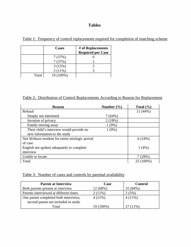
Tables

Table 1: Frequency of control replacements required for completion of matching scheme

Cases # of ReplacementsRequired per Case

7 (37%) 07 (37%) 13 (15%) 22 (11%) 3

Total 19 (100%)

Table 2: Distribution of Control Replacements According to Reason for Replacement

Reason Number (%) Total (%)Refusal 11 (44%) Simply not interested 7 (64%) Invasion of privacy 2 (18%) Family moving away 1 (9%) Their child’s interview would provide no new information to the study

1 (9%)

Not Woburn resident for entire etiologic periodof case

6 (24%)

English not spoken adequately to completeinterview

1 (4%)

Unable to locate 7 (28%)Total 25 (100%)

Table 3: Number of cases and controls by parental availability

Parent at Interview Case ControlBoth parents present at interview 12 (68%) 31 (84%)Parents interviewed at different times 2 (11%) 2 (5%)One parent completed both interviews, second parent not included in study

4 (21%) 4 (11%)

Total 19 (100%) 27 (11%)

Table 4: Distribution of cases by leukemia cell type

Cell Type Total Cases(%)

Participating Cases(%)

Acute Lymphoytic Leukemia (ALL) 17 (82) 15 (79)Acute Myelogenous Leukemia (AML) 3 (14) 3 (16)Chronic Myelogenous Leukemia (CML) 1 (5) 1 (5)

Total 21 (100) 19 (100)

Table 5 : Distribution by age category at diagnosis

Years of Age at Diagnosis Total Cases(%)

ParticipatingCases (%)

0 – 4 9 (43) 9 (47)5 – 9 4 (19) 3 (16)10-14 7 (33) 6 (32)

15 – 19 1 (5) 1 (5)Total 21 (100%) 19 (100%)

Table 6: Study subject frequency by exposure status and cumulative exposure to water from WellsG & H by exposure time period

Exposure Time Period ExposureCategory

CasesN=19# (%)

ControlsN=37# (%)

From 2 Years BeforeConception to Case Diagnosis(full etiologic period)

NeverEver

3 (15.8)16 (84.2)

13 (35.1)24 (64.9)

During 2 Years BeforeConception

NeverEver

11 (57.9)8 (42.1)

25 (67.6)12 (32.4)

During Pregnancy NeverEver

9 (47.4)10 (52.6)

25 67.612 (32.4 )

From Birth to Diagnosis NeverEver

7 (36.8)12 (63.2)

16 (43.2)21 (56.8)

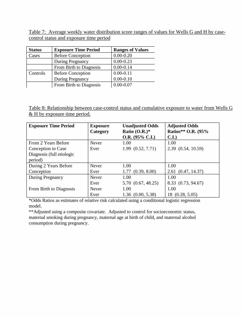
Table 7: Average weekly water distribution score ranges of values for Wells G and H by case-control status and exposure time period

Status Exposure Time Period Ranges of ValuesCases Before Conception 0.00-0.20

During Pregnancy 0.00-0.23From Birth to Diagnosis 0.00-0.14

Controls Before Conception 0.00-0.11During Pregnancy 0.00-0.10From Birth to Diagnosis 0.00-0.07

Table 8: Relationship between case-control status and cumulative exposure to water from Wells G& H by exposure time period.

Exposure Time Period ExposureCategory

Unadjusted OddsRatio (O.R.)*O.R. (95% C.I.)

Adjusted OddsRatios** O.R. (95%C.I.)

From 2 Years BeforeConception to CaseDiagnosis (full etiologicperiod)

NeverEver

1.001.99 (0.52, 7.71)

1.002.39 (0.54, 10.59)

During 2 Years BeforeConception

NeverEver

1.001.77 (0.39, 8.00)

1.002.61 (0.47, 14.37)

During Pregnancy NeverEver

1.005.70 (0.67, 48.25)

1.008.33 (0.73, 94.67)

From Birth to Diagnosis NeverEver

1.001.36 (0.00, 5.38)

1.0018 (0.28, 5.05)

*Odds Ratios as estimates of relative risk calculated using a conditional logistic regressionmodel.**Adjusted using a composite covariate. Adjusted to control for socioeconomic status,maternal smoking during pregnancy, maternal age at birth of child, and maternal alcoholconsumption during pregnancy.

Table 9A: Relationship between case-control status and cumulative exposure to water from WellsG & H by exposure time period.

Exposure TimePeriod

ExposureCategory

Unadjusted Odds Ratios(O.R.)*O.R. (95% C.I.)

Adjusted OddsRatios**O.R. (95% C.I.)

First Trimester NeverEver

1.002.29 (0.43, 12.23)

1.003.25 (0.47, 22.65)

Second Trimester NeverEver

1.005.70 (0.66, 49.20)

1.007.54 (0.70, 80.77)

Third Trimester NeverEver

1.007.03 (0.83, 59.53)

1.006.82 (0.77, 60.08)

*Odds ratios as estimates of relative risk calculated using a conditional logistic regressionmodel.**Adjusted using a composite covariate. Adjusted to control for socioeconomic status,maternal smoking during pregnancy, maternal age at birth of child, and maternal alcoholconsumption during pregnancy.

Table 9B: Correlation* coefficients between exposure to water from Wells G and H and trimesterof pregnancy.

Trimesters First Second ThirdFirst 1.00 0.76 0.67Second 0.76 1.00 0.84Third 0.67 0.84 1.00*Coefficients calculated using the Pearson product moment correlation.

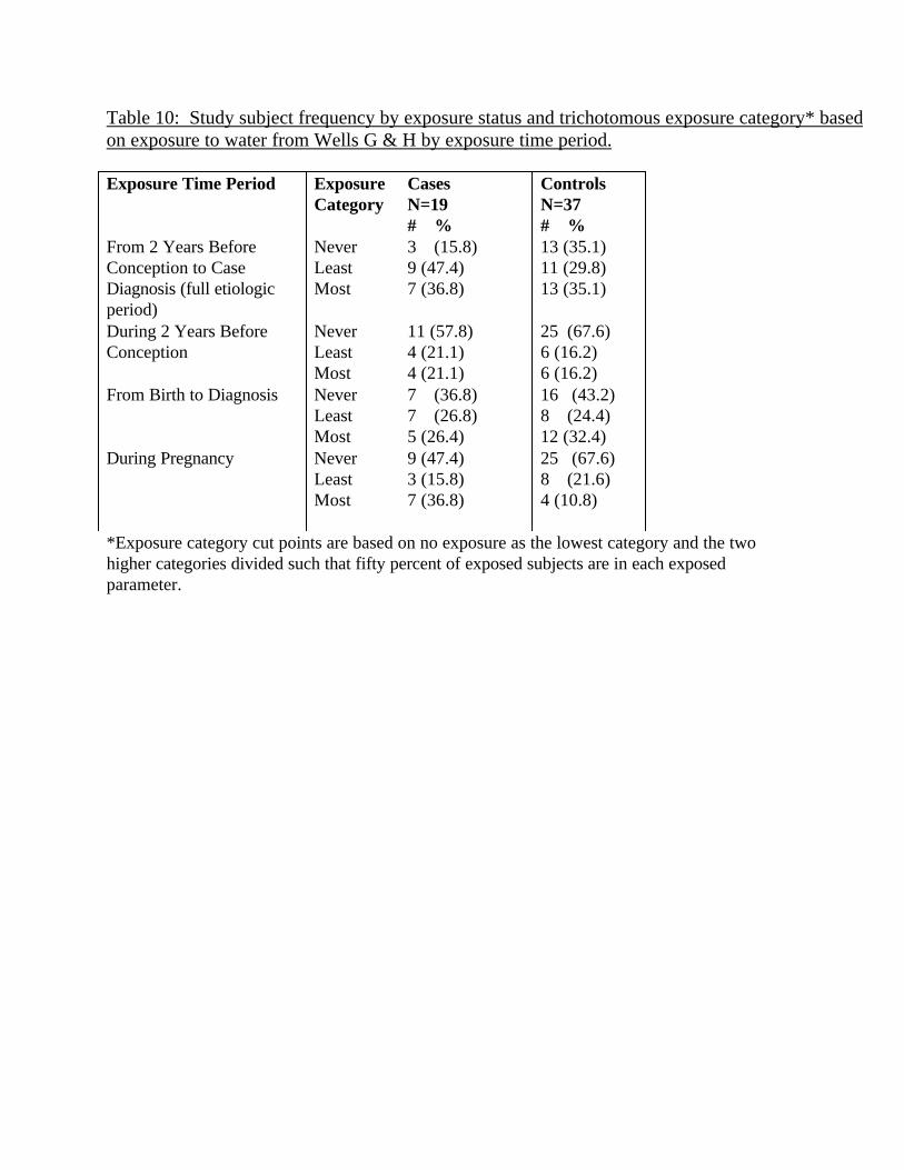
Table 10: Study subject frequency by exposure status and trichotomous exposure category* basedon exposure to water from Wells G & H by exposure time period.

Exposure Time Period ExposureCategory

CasesN=19# %

ControlsN=37# %

From 2 Years BeforeConception to CaseDiagnosis (full etiologicperiod)

NeverLeastMost

3 (15.8)9 (47.4)7 (36.8)

13 (35.1)11 (29.8)13 (35.1)

During 2 Years BeforeConception

NeverLeastMost

11 (57.8)4 (21.1)4 (21.1)

25 (67.6)6 (16.2)6 (16.2)

From Birth to Diagnosis NeverLeastMost

7 (36.8)7 (26.8)5 (26.4)

16 (43.2)8 (24.4)12 (32.4)

During Pregnancy NeverLeastMost

9 (47.4)3 (15.8)7 (36.8)

25 (67.6)8 (21.6)4 (10.8)

*Exposure category cut points are based on no exposure as the lowest category and the twohigher categories divided such that fifty percent of exposed subjects are in each exposedparameter.

Table 11: Relationship between case-control status and trichotomous exposure category* based onexposure to water from Wells G and H by exposure time period.

Exposure Time Period ExposureCategory

Unadjusted OddsRatios**O.R. (95% C.I.)

Adjusted *** OddsRatiosO.R. (95% C.I.)

From 2 Years BeforeConception to CaseDiagnosis (full etiologicperiod)

NeverLeastMost

1.003.52 (0.78, 26.41)2.41 (0.45, 13.01)

1.005.0 (0.75, 33.50)3.56 (0.51, 24.78)

During 2 Years BeforeConception

NeverLeastMost

1.001.82 (0.34, 9.64)1.68 (0.26, 11.04)

1.002.48 (0.42, 15.22)2.82 (0.30, 26.42)

From Birth to Diagnosis NeverLeastMost

1.002.24 (0.41, 12.37)0.98 (0.20, 4.71)

1.001.82 (0.31, 10.84)0.90 (0.18, 4.56)

During Pregnancy NeverLeastMost

1.002.36 (0.20, 28.48)14.00 (0.98, 195.60)

1.00****3.53 (0.22, 58.14)14.30 (0.92, 224.52)

*Exposure category cut points are based on no exposure as the lowest category and the twohigher categories divided such that fifty percent of exposed subjects are in each exposedparameter.**Odds Ratios as estimates of relative risk calculated using a conditional logistic regressionmodel.***Adjusted using a composite covariate. Adjusted to control for socioeconomic status,maternal smoking during pregnancy, maternal age at birth of child and maternal alcoholconsumption during pregnancy.****Test for trend is significant (P=0.045)

Table 12: Comparison of odds ratio* adjustment using a single composite covariate versus amultiple covariate adjustment logistic regression.

Exposure TimePeriod

ExposureScore

Adjusted Using aComposite Covariate**O.R. (95% C.I.)

Adjusted Using AllCovariates***O.R. (95% C.I.)

From 2 YearsBefore Conceptionto Case Diagnosis(full etiologicperiod)

NeverEver

1.002.39 (0.54, 10.5)

1.002.48 (0.53, 11.64)

During 2 YearsBefore Conception

NeverEver

1.002.61 (0.47, 14.3)

1.002.77 (0.51, 14.96)

From Birth toDiagnosis

NeverEver

1.001.18 (0.28, 5.05)

1.001.27 (0.29, 5.52)

During Pregnancy NeverEver

1.008.33 (0.73, 94.6)

1.0013.20 (0.85, 205.20)

*Odds Ratios as estimates of relative risk calculated using a conditional logistic regressionmodel.**Adjusted using a composite covariate. Adjusted to control for socioeconomic status,maternal smoking during pregnancy, maternal age at birth of child, and maternal alcoholconsumption during pregnancy.***Controlling for socioeconomic status, maternal smoking during pregnancy, maternal age atbirth of child, and maternal alcohol consumption, each covariate included as part of a singlelogistic regression model.

Table 13: Relationship between case-control status and exposure to water from Wells G and Hduring pregnancy for the total number for leukemias and by acute lymphocytic leukemias (ALL)only.

Leukemia Type Number ofCases

Odds Ratios 95% C.I.

Total Leukemias* AmongStudy Participants

19 5.69 (0.66, 49.20)

Acute LymphocyticLeukemia (ALL)

15 2.86 (0.30, 27.22)

*The total number of leukemias among study participants is composed of fifteen ALL cases,three ALL cases, and one CML case.

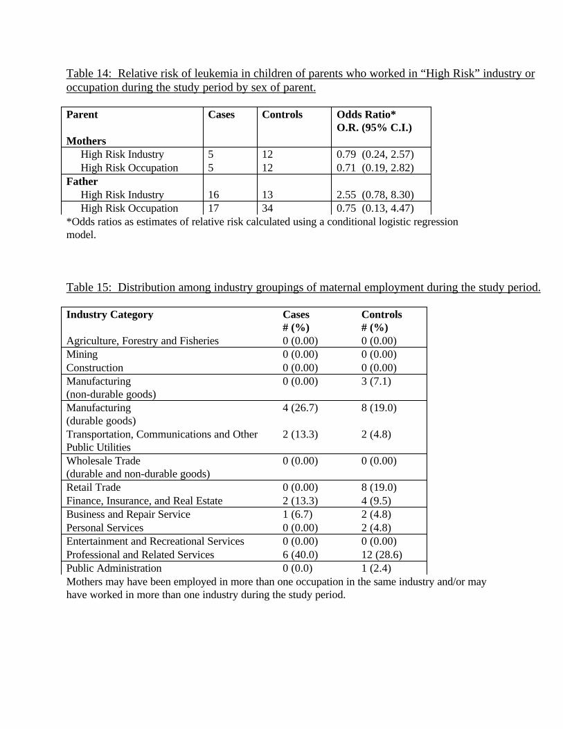
Table 14: Relative risk of leukemia in children of parents who worked in “High Risk” industry oroccupation during the study period by sex of parent.

Parent Cases Controls Odds Ratio*O.R. (95% C.I.)

Mothers High Risk Industry 5 12 0.79 (0.24, 2.57) High Risk Occupation 5 12 0.71 (0.19, 2.82)Father High Risk Industry 16 13 2.55 (0.78, 8.30) High Risk Occupation 17 34 0.75 (0.13, 4.47)*Odds ratios as estimates of relative risk calculated using a conditional logistic regressionmodel.

Table 15: Distribution among industry groupings of maternal employment during the study period.

Industry Category Cases# (%)

Controls# (%)

Agriculture, Forestry and Fisheries 0 (0.00) 0 (0.00)Mining 0 (0.00) 0 (0.00)Construction 0 (0.00) 0 (0.00)Manufacturing(non-durable goods)

0 (0.00) 3 (7.1)

Manufacturing(durable goods)

4 (26.7) 8 (19.0)

Transportation, Communications and OtherPublic Utilities

2 (13.3) 2 (4.8)

Wholesale Trade(durable and non-durable goods)

0 (0.00) 0 (0.00)

Retail Trade 0 (0.00) 8 (19.0)Finance, Insurance, and Real Estate 2 (13.3) 4 (9.5)Business and Repair Service 1 (6.7) 2 (4.8)Personal Services 0 (0.00) 2 (4.8)Entertainment and Recreational Services 0 (0.00) 0 (0.00)Professional and Related Services 6 (40.0) 12 (28.6)Public Administration 0 (0.0) 1 (2.4)Mothers may have been employed in more than one occupation in the same industry and/or mayhave worked in more than one industry during the study period.

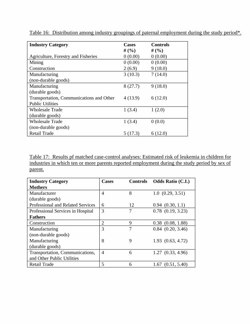
Table 16: Distribution among industry groupings of paternal employment during the study period*.

Industry Category Cases# (%)

Controls# (%)

Agriculture, Forestry and Fisheries 0 (0.00) 0 (0.00)Mining 0 (0.00) 0 (0.00)Construction 2 (6.9) 9 (18.0)Manufacturing(non-durable goods)

3 (10.3) 7 (14.0)

Manufacturing(durable goods)

8 (27.7) 9 (18.0)

Transportation, Communications and OtherPublic Utilities

4 (13.9) 6 (12.0)

Wholesale Trade(durable goods)

1 (3.4) 1 (2.0)

Wholesale Trade(non-durable goods)

1 (3.4) 0 (0.0)

Retail Trade 5 (17.3) 6 (12.0)

Table 17: Results pf matched case-control analyses: Estimated risk of leukemia in children forindustries in which ten or more parents reported employment during the study period by sex ofparent.

Industry Category Cases Controls Odds Ratio (C.I.)MothersManufacturer(durable goods)

4 8 1.0 (0.29, 3.51)

Professional and Related Services 6 12 0.94 (0.30, 1.1)Professional Services in Hospital 3 7 0.78 (0.19, 3.23)FathersConstruction 2 9 0.38 (0.08, 1.88)Manufacturing(non-durable goods)

3 7 0.84 (0.20, 3.46)

Manufacturing(durable goods)

8 9 1.93 (0.63, 4.72)

Transportation, Communications,and Other Public Utilities

4 6 1.27 (0.33, 4.96)

Retail Trade 5 6 1.67 (0.51, 5.40)

Table 18: Distribution among occupational groupings of maternal employment during the studyperiod*.

Occupational Category Cases# (%)

Controls# (%)

Managerial and Professional Specialty OccupationsExecutive, Administrative, and Managerial Occupation 2 (7.4) 1 (1.9)Professional Specialty Occupations 0 (0.0) 0 (0.0)Technical, Sales and Administrative Support OccupationsTechnicians and Related Support Occupations 2 (7.4) 1 (1.9)Sales Occupations 0 (0.0) 0 (0.0)Administrative Support Occupations 7 (25.9) 10 (18.9)Service OccupationsPrivate Household Occupations 0 (0.0) 0 (0.0)Protective Service Occupations 0 (0.0) 0 (0.0)Other Service Occupations 1 (3.7) 6 (11.3)Farming, Forestry and Fishing OccupationsPrecision Production, Craft and Repair OccupationsMechanics and Repairers

0 (0.0) 0 (0.0)

Construction Trades 0 (0.0) 0 (0.0)Extractive Operations 0 (0.0) 0 (0.0)Precision Production Operations 0 (0.0) 2 (3.8)Operators, Fabricators and LaborersMachine Operators, Assemblers and Inspectors 0 (0.0) 2 (3.8)Transportation and Material Moving Operations 0 (0.0) 2 (3.8)Handlers, Equipment Cleaners, Helpers and Laborers 0 (0.0) 1 (1.9)Homemakers 15 (55.6) 28 (52.7)*Mothers may have been employed in more than one occupation in the same industry and/ormay have worked in more than one industry during the study period.

Table 19: Distribution among occupational groupings of paternal employment during the studyperiod*.

Occupational Category Cases# %

Controls# %

Managerial and Professional Specialty OccupationsExecutive, Administrative, and Managerial Occupation 3 (10.7) 7 (13.7)Professional Specialty Occupations 4 (14.4) 7 (13.7)Technical, Sales and Administrative Support OccupationsTechnicians and Related Support Occupations 2 (7.1) 6 (11.8)Sales Occupations 3 (10.7) 6 (11.8)Administrative Support Occupations 3 (10.7) 3 (5.9)Service OccupationsPrivate Household Occupations 0 (0.0) 0 (0.0)Protective Service Occupations 3 (10.7) 0 (0.0)Other Service Occupations 0 (0.0) 0 (0.0)Farming, Forestry and Fishing Occupations 0 (0.0) 2 (3.9)Precision Production, Craft and Repair OccupationsMechanics and Repairers

0 (0.0) 2 (3.9)

Construction Trades 3 (10.7) 6 (11.8)Extractive Operations 0 (0.0) 0 (0.0)Precision Production Operations 1 (3.7) 3 (5.9)Operators, Fabricators and LaborersMachine Operators, Assemblers and Inspectors 2 (7.1) 3 (5.9)Transportation and Material Moving Operations 2 (7.1) 3 (5.9)Handlers, Equipment Cleaners, Helpers and Laborers 2 (7.1) 3 (5.9)*Fathers may have been employed in more than one occupation in the same industry and/or mayhave worked in more than one industry during the study period.

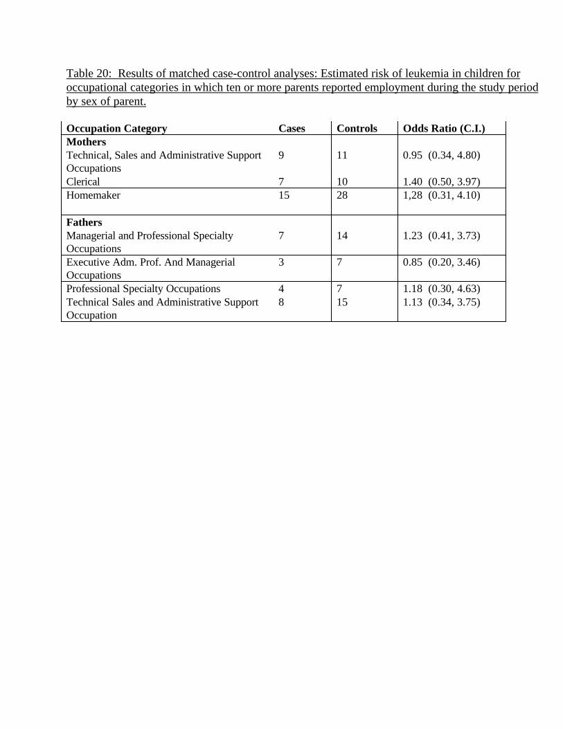
Table 20: Results of matched case-control analyses: Estimated risk of leukemia in children foroccupational categories in which ten or more parents reported employment during the study periodby sex of parent.

Occupation Category Cases Controls Odds Ratio (C.I.)MothersTechnical, Sales and Administrative SupportOccupations

9 11 0.95 (0.34, 4.80)

Clerical 7 10 1.40 (0.50, 3.97)Homemaker 15 28 1,28 (0.31, 4.10)

FathersManagerial and Professional SpecialtyOccupations

7 14 1.23 (0.41, 3.73)

Executive Adm. Prof. And ManagerialOccupations

3 7 0.85 (0.20, 3.46)

Professional Specialty Occupations 4 7 1.18 (0.30, 4.63)Technical Sales and Administrative SupportOccupation

8 15 1.13 (0.34, 3.75)

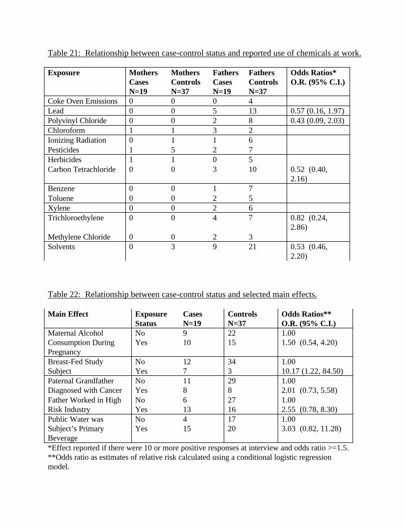
Table 21: Relationship between case-control status and reported use of chemicals at work.

Exposure MothersCasesN=19

MothersControlsN=37

FathersCasesN=19

FathersControlsN=37

Odds Ratios*O.R. (95% C.I.)

Coke Oven Emissions 0 0 0 4Lead 0 0 5 13 0.57 (0.16, 1.97)Polyvinyl Chloride 0 0 2 8 0.43 (0.09, 2.03)Chloroform 1 1 3 2Ionizing Radiation 0 1 1 6Pesticides 1 5 2 7Herbicides 1 1 0 5Carbon Tetrachloride 0 0 3 10 0.52 (0.40,

2.16)Benzene 0 0 1 7Toluene 0 0 2 5Xylene 0 0 2 6Trichloroethylene 0 0 4 7 0.82 (0.24,

2.86)Methylene Chloride 0 0 2 3Solvents 0 3 9 21 0.53 (0.46,

2.20)

Table 22: Relationship between case-control status and selected main effects.

Main Effect ExposureStatus

CasesN=19

ControlsN=37

Odds Ratios**O.R. (95% C.I.)

Maternal AlcoholConsumption DuringPregnancy

NoYes

910

2215

1.001.50 (0.54, 4.20)

Breast-Fed StudySubject

NoYes

127

343

1.0010.17 (1.22, 84.50)

Paternal GrandfatherDiagnosed with Cancer

NoYes

118

298

1.002.01 (0.73, 5.58)

Father Worked in HighRisk Industry

NoYes

613

2716

1.002.55 (0.78, 8.30)

Public Water wasSubject’s PrimaryBeverage

NoYes

415

1720

1.003.03 (0.82, 11.28)

*Effect reported if there were 10 or more positive responses at interview and odds ratio >=1.5.**Odds ratio as estimates of relative risk calculated using a conditional logistic regressionmodel.

Table 23: Maternal employment outside the home and its relation to case-control status bysegment of the etiologic period.

Time Period ** Cases Controls Odds Ratio*O.R. (C.I.)

3 Months Before Conception 10 16 1.59 (0.47, 5.46)During First Trimester 8 18 0.59 (0.42, 2.56)During Second Trimester 6 17 0.45 (0.11, 1.86)During Third Trimester 6 13 0.86 (0.23, 3.26)*Odds ratios as estimates of relative risk calculated using a conditional logistic regressionmodel.**Mothers may have been employed in more than one time period.

Table 24: Distribution of all residences by four level wire configuration code and disease status.

Wire Code Cases# (%)

Controls# (%)

Totals# (%)

VHCC 2 (10.6) 6 (11.1) 8 (11.0)OHCC 2 (10.5) 12 (22.2) 14 (19.2)OLCC 14 (73.7) 32 (59.3) 46 (63.0)VLCC 1 (5.3) 4 (7.4) 5 (6.8)Total 19 (100.0) 54 (100.0) 73 (100.0)

Table 25: Distribution of all stable residences by four level wire configuration code and diseasestatus

Wire Code Cases# (%)

Controls# (%)

Total# (%)

VHCC 1 (6.7) 3 (12.5) 4 (10.2)OHCC 2 (13.3) 3 (12.5) 5 (12.8)OLCC 12 (80.0) 16 (66.7) 28 (71.9)VLCC 1 (0.0) 2 (8.3) 2 (5.1)Total 15 (100.0) 24 (100.0) 39 (100.0)

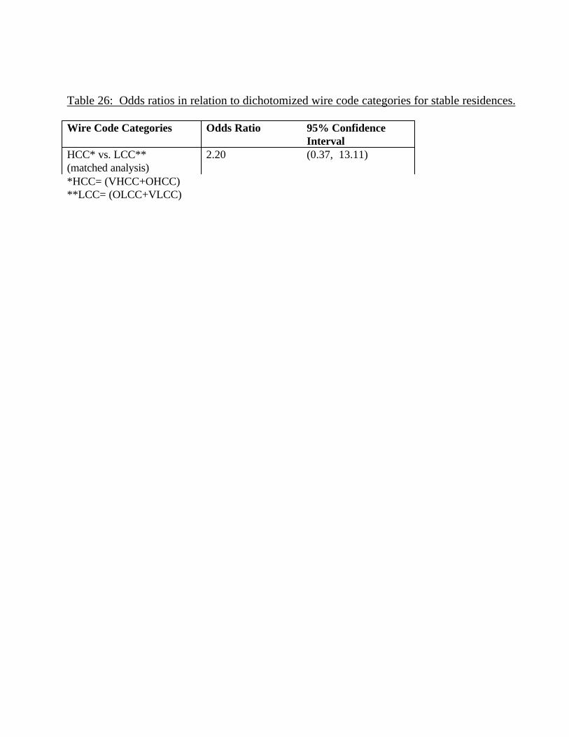
Table 26: Odds ratios in relation to dichotomized wire code categories for stable residences.

Wire Code Categories Odds Ratio 95% ConfidenceInterval

HCC* vs. LCC**(matched analysis)

2.20 (0.37, 13.11)

*HCC= (VHCC+OHCC)**LCC= (OLCC+VLCC)