Wireless Sensor Network for Temperatures Estimation in an

ACTA IMEKO ISSN: 2221-870X March 2018, Volume 7, Number 1, 5-12

ACTA IMEKO | www.imeko.org March 2018 | Volume 7 | Number 1 | 5

Wireless Sensor Network for Temperatures Estimation in an Asynchronous Machine Using a Kalman Filter Yi Huang, Clemens Gühmann

Technische Universität Berlin, Chair of Electronic Measurement and Diagnostic Technology, Sekr. EN13 Einsteinufer 17, D-10589 Berlin, Germany

Section: RESEARCH PAPER

Keywords: Kalman filter; temperature estimation; asynchronous machine; thermal losses; wireless sensor network

Citation: Yi Huang, Clemens Gühmann, Wireless Sensor Network for Temperatures Estimation in an Asynchronous Machine Using a Kalman Filter, Acta IMEKO, vol. 7, no. 1, article 3, March 2018, identifier: IMEKO-ACTA-07 (2018)-01-03

Section Editor: Lorenzo Ciani, University of Florence, Italy

Received September 24, 2017; In final form November 29, 2017; Published March 2018

Copyright: © 2018 IMEKO. This is an open-access article distributed under the terms of the Creative Commons Attribution 3.0 License, which permits unrestricted use, distribution, and reproduction in any medium, provided the original author and source are credited

Funding: This work was supported by Chair of Electronic Measurement and Diagnostic Technology, Technische Universitäte Berlin

Corresponding author: Yi Huang, e-mail: [email protected]

1. INTRODUCTION

The WSNs consist of sensor nodes including power module, data processing module, wireless module and other peripherals for untethered communication. Many applications such as the monitoring of the environment, the industry and the medical care are used based on WSN. The signals acquired and pre-processed by a wireless sensor node will be transmitted to the host sensor node and be processed there. This project is focused on the monitoring algorithm implementation in a WSN. Because of the restrictions of the sensor nodes, such as low cost, low power, weak computation power and small memory size, many challenges have to be solved by the implementation. The temperature monitoring system of an asynchronous machine was examined for the implementation of the algorithm on WSN.

Due to the characteristics, such as low cost, robustness and

low maintenance, asynchronous machines are widely used in industrial and electrical vehicles. The thermal behavior of an asynchronous machine largely determines the maximum lifetime, the ability of over-load and the accuracy in high-performance controller [1]. The high temperature, which is exceeding the service limit, may result in insulation deterioration as well as rotor faults [2]. As a result, the temperature monitoring of the stator winding, the rotor cage and the stator core, can be used to initiate certain reactions in order to circumvent thermal fault and predictive monitoring. It can protect the machine, extend the life span and contribute to the high performance of the machine [2].

Generally, three methods can be employed for the temperature monitoring. A direct way is that the temperature can be measured by using mounted sensor. It is possible to fix a sensor on the surface of the stator core and inside the stator

ABSTRACT A 4th-order Kalman filter (KF) algorithm is developed based on the thermal model of an asynchronous machine. The thermal parameters are identified and KF is implemented in a wireless sensor network (WSN) to estimate the temperatures of the stator windings, the rotor cage, and the stator core of an asynchronous machine. The rotor speed, coolant air temperature, and the effective current and voltage are acquired by a WTIM (wireless transducer interface module) separately and transmitted to a NCAP (network capable application processor) where the KF algorithm is implemented. Losses of the stator windings and the rotor cage are copper losses, and the stator core losses are iron losses. The losses of the stator windings, the rotor cage and the stator core are calculated from the measurements and are processed with the coolant air temperature by KF. As the resistance varies with temperature, the estimated temperature of the stator windings is used for compensating the rising of resistance. Simulations and experiments on the test bench were performed prior to the KF algorithm is implemented on a wireless sensor node. The real-time temperature estimator on WSN is independent from control algorithm and can work under any load condition with very high accuracy.


winding. The temperature of the rotor cage can be acquired using WSN, but the high cost and the instability of the measurement system make it unsuitable for industrial usage [21]. The second way is that the temperatures of the stator winding and the rotor cage can be calculated by identifying the resistance, because it is a temperature dependent variable. A sensor-less internal temperature monitoring method for induction motor was introduced [1]. The author in [5] proposes a method to estimate the rotor and stator temperatures using extended Kalman filter, when satisfying the assumption that there is no temperature rising for the coolant air temperature. The authors in [3] present an approach to estimate temperatures based on a thermal model. Thermal analysis based on lumped-parameter thermal network, finite-element analysis, and computational fluid dynamics were considered. The design of a state-of-the-art rotor temperature monitoring system for contact measurement was proposed in [4].

Building the thermal model of an electric machine is a complex multi-disciplinary problem, and it must evaluate the main internal losses of the machine, also [6]. The most frequently estimation techniques rely on a calculation of the resistance in steady state [7], [8]. The estimation of the stator resistance and rotor resistance has been presented in [5] and [9], but neither of them estimates the resistance simultaneously.

This paper describes the implementation of a temperature monitoring system in a WSN using a Kalman filter. The temperatures are estimated directly based on the thermal model of the asynchronous machine. The state-space of the system is presented in section II. Objected-modelling and parameter identification are introduced in section III. Section IV illustrates the KF algorithm and the tuning of the covariance matrix. In section V, the Model-in-the-Loop (MiL) method is used for simulation and KF algorithm verification in SIMULINK and the experiment results are described. Section VI discusses the implementation of the KF on the wireless sensor node. Finally, the conclusions are given in the last section.

2. THE THERMAL MODEL OF THE ASYNCHRONOUS MACHINE

Heat transfer in the machine can be simplified as heat conduction in the solid parts and convection in the boundary layer of flowing medium. However, radiation is not considered in this paper. The thermal network is analogous to an electrical network, as temperature to voltage, power to current, thermal resistance to electrical resistance and thermal capacitance to electrical capacitance. By summarizing the structure of the machine, the thermal network is shown in Figure 1.

2.1. The state-space equations A lumped-parameter thermal circuit is built based on the

losses balance theory and the simplified thermal model in Figure 1, the state-space can be defined as following equations: 𝑑𝑇𝑠𝑠𝑑𝑑

= −𝑅𝑠𝑠𝑇𝑠𝑠𝐶𝑠𝑠

+ 𝑅𝑠𝑠𝑇𝑠𝑠𝐶𝑠𝑠

+ 𝑃𝑠𝑠𝐶𝑠𝑠

(1)

𝑑𝑇𝑟𝑠𝑑𝑑

= −𝑅𝑟𝑠𝑇𝑟𝑠𝐶𝑟𝑠

+ 𝑅𝑟𝑠𝑇𝑠𝑠𝐶𝑟𝑠

+ 𝑃𝑟𝑠𝐶𝑟𝑠

(2)

𝑑𝑇𝑠𝑠𝑑𝑑 =

−𝑅𝑠𝑠𝑇𝑠𝑠𝐶𝑠𝑠

+𝑅𝑟𝑠𝑇𝑟𝑠𝐶𝑠𝑠

+𝑅𝑠𝑠𝑇𝑠𝐶𝑠𝑠

+ (𝑅𝑠𝑠+𝑅𝑟𝑠+𝑅𝑠𝑠)𝑇𝑠𝑠

𝐶𝑠𝑠+ 𝑃𝑠𝑠

𝐶𝑠𝑠 (3)

where 𝑇𝑠𝑠 ,𝑇𝑟𝑠 ,𝑇𝑠𝑠 ,𝑇𝑠 indicate the temperature above ambient of the stator winding, the rotor cage, the stator core and the coolant air respectively. 𝑅𝑠𝑠,𝑅𝑟𝑠 ,𝑅𝑠𝑠 are the thermal resistance of the stator winding, the rotor cage and the stator core. 𝐶𝑠𝑠 ,𝐶𝑟𝑠,𝐶𝑠𝑠 indicate the thermal capacitances of the stator wingding, the rotor cage and the stator core. 𝑃𝑠𝑠 ,𝑃𝑟𝑠 ,𝑃𝑠𝑠 are the power losses of the stator winding, the rotor cage and the stator core.

In the simplified thermal model, 𝑃𝑠𝑠 , 𝑃𝑟𝑠 are ohmic losses, and 𝑃𝑠𝑠 is the frequency-dependent iron loss, 𝑅𝑠 and 𝑅𝑟 are resistances in ohm, between any two-line terminals, 𝜔𝑚 is the mechanical speed of the rotor in rad/s, 𝑘𝑖𝑟𝑖𝑖 is the iron loss constant which is given in Table 3. The losses can be represented as:

𝑃𝑠𝑠(𝑑) = 𝐼𝐿2(𝑑)𝑅𝑠(𝑇𝑠𝑠(𝑑)) (4)

𝑃𝑠𝑠(𝑑) = 𝑘𝑖𝑟𝑖𝑖𝜔𝑚2 (5)

As the current of the rotor is not available to be measured or to be estimated using simple method, the rotor cage losses can be calculated indirectly which is defined in IEEE Power Engineering Society's publication [12]. 𝑃𝑟𝑠(𝑑) = (𝑃𝑖𝑖(𝑑) − 𝑃𝑠𝑠(𝑑) − 𝑃𝑠𝑠(𝑑))𝑠(𝑑) (6)

𝑃𝑖𝑖(𝑑) = 3𝑈𝐿(𝑑)𝐼𝐿(𝑑) cos∅ (7)

𝑠(𝑑) = 𝜔𝑠−𝜔𝑟(𝑑)𝜔𝑠

(8)

where 𝑃𝑖𝑖 is the input power of the machine, 𝑈𝐿 and 𝐼𝐿 are the line voltage and the line current, respectively. 𝜔𝑠 is the synchronous speed, 𝜔𝑟 is the rotor speed, 𝑠 is the slip of the machine and 𝑐𝑐𝑠 ∅ is the power factor.

The temperatures of the stator winding and rotor cage increase largely, which leads 40 % rising of the reference resistances. As a result, the temperature dependent characteristic of the resistance is used to compensate the ignored increasing resistance. All in all, the stator winding losses can be calculated much more accurately. 𝑅𝑠 can be replaced by the following equation: 𝑅𝑠(𝑑) = 𝑅𝑠𝑅𝑠𝑠(𝑑)(1 + 𝛼𝑠𝑇𝑠𝑠(𝑑)) (9)

where 𝑅𝑠𝑅𝑠𝑠 is the stator winding resistance at the reference temperature. The 𝛼𝑠 is the copper temperature coefficient of

Psw PscPrc

Csw Crc Csc

Rsw Rrc

Rsc Coolant air

Tsw Trc Tsc Figure 1. Thermal network of the asynchronous machine.


stator winding with the value of 0.004041.

2.2. Definition of the system The state-space equations of the system can be acquired by calculating the losses 𝑃𝑠𝑠 , 𝑃𝑟𝑠 and 𝑃𝑠𝑠 which are defined in equations (4) - (6), and importing them into equations (1) - (3). By summarizing the previous equations, the system can be rewritten as a 4th-order linear continuous time-invariant system in the state space model form: 𝒙′(𝑑) = 𝐴𝒙(𝑑) + 𝐵𝒖(𝑑) (10) 𝒛(𝑑) = 𝐶𝒙(𝑑) + 𝐷𝒖(𝑑) (11) where: 𝒙 = [𝑇𝑠𝑠 ,𝑇𝑟𝑠 ,𝑇𝑠𝑠 ,𝑇𝑠]𝑇 (12) 𝒛 = 𝑇𝑠 (13) 𝒖 = [𝑃𝑠𝑠 ,𝑃𝑟𝑠 ,𝑃𝑠𝑠 , 0]𝑇 (14)

𝐴 =

⎣⎢⎢⎢⎢⎡−𝑅𝑠𝑠𝐶𝑠𝑠

0 𝑅𝑠𝑠𝐶𝑠𝑠

0

0 −𝑅𝑟𝑠𝐶𝑟𝑠

𝑅𝑟𝑠𝐶𝑟𝑠

0𝑅𝑠𝑠𝐶𝑠𝑠

𝑅𝑟𝑠𝐶𝑠𝑠

−(𝑅𝑠𝑠+𝑅𝑟𝑠+𝑅𝑠𝑠)𝐶𝑠𝑠

𝑅𝑠𝑠𝐶𝑠𝑠

0 0 0 0 ⎦⎥⎥⎥⎥⎤

(15)

𝐵 =

⎣⎢⎢⎢⎢⎡1𝐶𝑠𝑠

0 0 0

0 1𝐶𝑟𝑠

0 0

0 0 1𝐶𝑠𝑠

00 0 0 0⎦

⎥⎥⎥⎥⎤

(16)

𝐶 = 1 (17) 𝐷 = 0 (18)

In the state equations, 𝒙(𝒕) is the state vector, 𝒖(𝒕) is the control vector. The matrices 𝑨 and 𝑩 are constant coefficient which are the system transition matrix and the input matrix respectively. In the measurement equation, 𝑪 is the output matrix, which is a constant in this system. 𝑫 is the feedthrough matrix, which is zero. The coolant air temperature 𝑻𝒄 is considered a constant parameter due to the slow variation with time.

3. OBJECTED-ORIENTED MODELLING AND PARAMETER IDENTIFICATION

Model-based algorithm development method firstly relies on the physical model of the system, which can be used for the validation of the proposed temperature estimation algorithm. The physical model is developed to simulate the characteristics of the asynchronous machine, including the mechanical, electrical and thermodynamic characteristics.

3.1. Modelling of an Asynchronous Machine with a simplified Thermal Model

The physical model consists of two parts in Modelica® [13]. One is the squirrel cage asynchronous machine with six types of losses which is provided by the Modelica standard library, and the other is the simplified thermal model. The electronic and magnetic behaviours as well as six parts of the machine losses can be simulated with the asynchronous machine model. Figure 2 shows the simplified thermal model, which is based on the Figure 1. The heat sources of the machine are from the red

thermal port, where imports the losses of stator winding 𝑷𝒔𝒔, the rotor cage 𝑷𝒓𝒄, the stator core 𝑷𝒔𝒄, the rotor core, friction losses and stray load losses into the thermal circuit [11]. There is no core in the squirrel cage rotor, so the losses of the rotor core are zero. The friction losses and the stray load losses, which are not contributed to the thermal transfer, are dissipated to the environment. The mentioned three parts are represented as “rotorCore”, “fiction” and “strayload” in Figure 2. The components named in “CstatorWinding”, “CrotorCage”, “CstatorCore” are capacitors respectively. The components named in “GstatorWinding”, “GrotorCage”, “GstatorCore” are the reciprocal of resistances respectively. The blue components below are the air cooling system. Power losses are injected into the thermal model by enabling an internal thermal port of the machine model. All the losses can be imported to the thermal network. The complex simulation model in Figure 3 is built in Dymola [14], where the dynamic behaviour of the system can be simulated. The temperatures of stator windings, the rotor cage and the stator core can be simulated by the thermal model.

3.2. Parameter Identification of the Model The parameters of the test bench are identified in [15], [16]. The parameters of the asynchronous machine are listed in Table 3 in appendix. The thermal resistances can be calculated directly

Figure 3. Asynchronous machine and simplified thermal model.

Figure 2. Simplified thermal model.


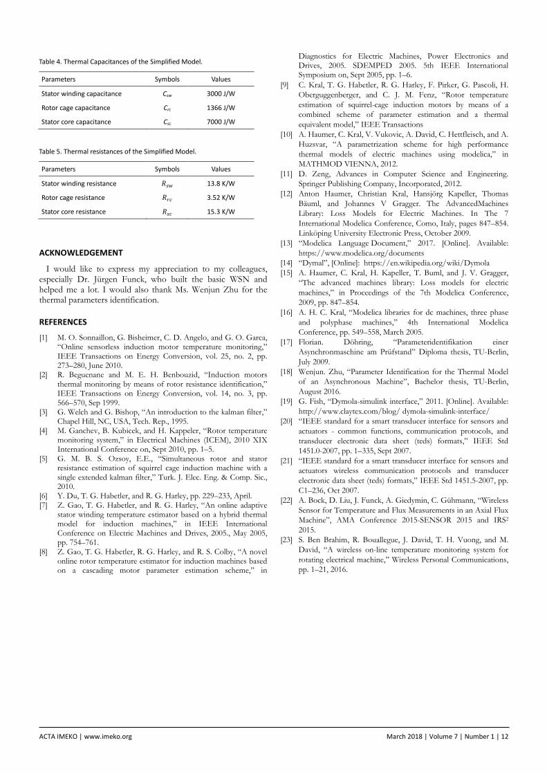
based on the state-space equations (1) (2) (3). Full-load test are performed to identify the thermal resistances. After the heat exchanges among ambient and machine’s components are stable, the derivatives of temperature with respect to time will be zero. By measuring the end temperature of 𝑇𝑠𝑠 , 𝑇𝑟𝑠 , 𝑇𝑠𝑠 and 𝑇𝑠 and calculating of power losses in machine, the resistances can be derived from the equations (1) (2) (3). Table 4 lists the thermal resistances. The thermal capacitances cannot be computed directly from the equations (1) (2) (3). However, it is possible to utilize optimization methods to determine the best-fit thermal capacitances using GenOpt, an optimization program for the minimization of a cost function. The detailed description of the capacitance identification can be referred to a bachelor thesis. Table 5 lists the capacitances.

3.3. Validation of the model The model must be at first validated for the simulation. The

literature [19] provides several methods to prove the validity of the presented load models, which are all relied on the mechanical output power. Generally, the torque-speed (or torque-slip) characteristics of a three-phase asynchronous machine can also indicate the motor performance at any rotor operating speed according to [20]. Therefore, four different characteristic curves of the measurement and the simulation results are shown in Figure 4 under various load torque. The first three characteristic curves in Figure 4 show good coincidence of the simulated curve and measured one. Nevertheless, it is also to be noticed, that simulated input current is a little bit higher than the measured one, which may lead to excessive temperature rising in the thermal model.

Thermal model plays an important role in temperature monitoring. Combined together with the asynchronous machine model, the validation of the thermal model is performed. All the machine and thermal model related parameters are set to be the identified parameters based on the test bench. Two experiments are tested for the model validation. One is the continuous full-load S1 and the other is the intermittent load S6 which aims to confirm that the thermal model could also represent the temperature of asynchronous machine under other load conditions. The temperatures of the machine on the test bench are measured and compared with the simulated temperatures in the model. The comparisons indicate that the physical model can be used for model-based algorithm

development, which will be introduced in section 5.

4. KALMAN FILTER ALGORITHM

Kalman filter is a set of mathematical equations that provides an efficient computational (recursive) means to estimate the state of a process, in a way that minimizes the mean of the squared error [3]. In general, both the process noise and the measurement noise should be taken into account in the system model and measurement model.

𝑥(𝑘 + 1) = 𝑓(𝑥(𝑘),𝑢(𝑘)) + 𝜔(𝑘) (19)

𝑧(𝑘) = ℎ𝑥(𝑘) + 𝑣(𝑘) (20)

It is assumed that the process noise 𝜔𝑘and the measurement noise 𝑣𝑘 are independent of each other, random white Gaussian noise with zero mean. Their variance can be described by covariance matrices 𝑄 and 𝑅 respectively. They can be defined as:

𝐸[𝜔𝑘𝜔𝑘𝑇] = 𝑄 (21)

𝐸[𝑣𝑘𝑣𝑘𝑇] = 𝑅 (22)

where 𝑄 is a 4×4 positive semi-defined constant matrix and 𝑅 is constant.

4.1. The Prediction Stage of Kalman Filter Kalman filter estimates a process by using a feedback control:

the filter estimates the process state at some time and then obtains feedback in the form of (noisy) measurements [3]. As such, the equations of Kalman filter can be divided into two groups: prediction equations and correction equations.

The equations of prediction stage shown in (23) and (24) are responsible for projecting forward (in time) the current state and error covariance estimates to obtain a priori estimates for the next time step. Equation (23) is used for updating the state vector from previous sampling time 𝒌 − 𝟏to current time 𝒌. The equation (24) is state of updating error covariance matrix.

𝒙�𝒌− = 𝑨𝒅𝒙�𝒌−𝟏− + 𝑩𝒅𝒖𝒌−𝟏 (23)

𝑷�𝒌− = 𝑨𝒅𝑷𝒌−𝟏𝑨𝒅𝑻 + 𝑸 (24)

The model (10) (11) is a time-continuous system which cannot be processed by computer. Euler's approximation is used to discrete the model, so that the sampled data can be used in the KF algorithm. The discrete of the system can be defined as equation (25) 𝒙(𝒌)−𝒙(𝒌−𝟏)

𝝉= 𝑨𝒙(𝒌 − 𝟏) + 𝑩𝒖(𝒌 − 𝟏) (25)

By simplifying the equation (25), a new equation can be expressed as: 𝑥(𝑘) = (1 + 𝜏𝐴)𝑥(𝑘 − 1) + 𝜏𝐵𝑢(𝑘 − 1) (26)

As 𝐴 and 𝐵 are the matrix, the time-discrete model is 𝑥(𝑘) = 𝐴𝑑𝑥(𝑘 − 1) + 𝐵𝑑𝑢(𝑘 − 1) (27)

where 𝐴𝑑 = 𝐸 + 𝜏𝐴 and 𝐵𝑑 = 𝜏𝐵, 𝐸 is 4×4 unit matrix, 𝐶𝑑 is equal to 𝐶, 𝜏 is the sampling time.

Ad =

⎣⎢⎢⎢⎢⎡1 −

RswτCsw

0 RswτCsw

0

0 1 − RrcτCrc

RrcτCrc

0RswτCsc

RrcτCsc

1 − (Rsw+Rrc+Rsc)τCsc

RscτCsc

0 0 0 1 ⎦⎥⎥⎥⎥⎤

(28)

Figure 4. Thermal network of the asynchronous machine.

0 1000 2000 3000 40002

4

6

8mechanical power-current

Pmech/W

curre

nt/A

simulatedmeasured

0 1000 2000 3000 40001400

1450

1500speed-mechanical power

Pmech/W

spee

d/rp

m

simulatedmeasured

0 1000 2000 3000 40000

0.5

1mechanical power-efficiency

Pmech/W

powe

r effi

cienc

y

simulatedmeasured

1400 1450 15000

10

20

30speed-torque

speed/rpm

torq

ue/N

.m

simulatedmeasured


Bd =

⎣⎢⎢⎢⎢⎡τ

Csw0 0 0

0 τCrc

0 0

0 0 τCsc

00 0 0 0⎦

⎥⎥⎥⎥⎤

(29)

4.2. The Correction stage of KF

The equations of correction stage are responsible for the feedback-i.e. for incorporating a new measurement into a priori estimation to obtain an improved a posteriori estimation [3].

𝐾𝑘 = 𝑃𝑘−𝐻𝑘𝑇(𝐻𝑘𝑃𝑘−𝐻𝑘𝑇 + 𝑅)−1 (30)

𝑥�𝑘 = 𝑥�𝑘− + 𝐾𝑘(𝑧𝑘 − 𝐻𝑘𝑥�𝑘−) (31)

𝑃𝑘 = (𝐼 − 𝐾𝑘𝐻𝑘)𝑃𝑘− (32)

where 𝐾𝑘 is Kalman gain and is the measurement matrix 𝐻𝑘 is a row vector [0,0,0,1].

5. MODEL IN THE LOOP (MIL) SIMULATION AND TEST

The asynchronous machine model, connected with the simplified thermal model in Dymola is compiled as a DymolaBlock in SIMULINK. The DymolaBlock and the KF algorithm block are simulated in SIMULINK.

5.1. The Simulation Model in SIMULINK The combined model in Dymola is compiled as a

DymolaBlock in Simulink. The configuration and implementation of the Dymola model in Simulink is described in detail by Garron Fish [19]. KF algorithm is implemented as an S-Function, and connected with the DymolaBlock in Matlab/Simulink. In the complete simulation model, three-phase stator currents are the measurement. Three-phase voltages and the coolant air temperature are the control vectors. All of them can be exported from DymolaBlock as the input of KF. The estimated temperatures from KF can be compared with the temperature calculated by the simplified thermal model. The whole simulation model in Simulink is shown in Figure 5.

5.2. The MiL Simulation of KF Algorithm

The temperatures of the stator wingding, the rotor cage and the stator core can be estimated in any operating condition. For all the experiments, fixed simulation step is set to 0.1 ms. The sampling time, which is set by Rate Transition block, is 1 s. The initial error covariance matrix, process noise covariance matrix, and measurement covariance matrix are obtained by trial and

error method:

𝑷(𝟎) = 𝒅𝒅𝒅𝒅[𝟐𝟎 𝟐𝟎 𝟐𝟎 𝟐𝟎]

𝑸 = 𝒅𝒅𝒅𝒅[𝟎.𝟎𝟎𝟏 𝟎.𝟎𝟎𝟏 𝟎.𝟎𝟎𝟏 𝟎.𝟏]

𝑹 = 𝟎.𝟏 From the state-space equations (1) - (3), losses of the thermal model largely determine the accuracy of the estimated temperatures. In order to prove the assumption, we proposed three different methods to get losses when the whole system is running. It is expected that the deviations between the simulated and estimated temperatures would be less than 1 K. The first method is to export losses directly from the DymolaBlock to Kalman filter. The second is to calculate the losses based on the equations (4) - (8), where 𝑅𝑠 is taken as a constant. The third method is to calculate the losses as the same as in the second method, but the difference is that for every simulation step, the estimated temperature of stator winding 𝑇𝑠𝑠 would be sent back to losses calculation block to compensate the ignored stator winding resistance rising defined in equation (9). For every method, two experiments are performed. One is the continuous full-load S1, which means that the machine runs at the rated condition until the temperatures of three-parts reach stable. The other experiment is called S6, which is an intermittent load with six minutes no-load followed by four minutes 140 % full-load.

5.2.1. The Estimation Results by Exported Losses from Dymola.

Losses of the stator windings 𝑷𝒔𝒔, rotor cage 𝑷𝒓𝒄 and stator core 𝑷𝒔𝒄 are exported from DymolaBlock and sent to KF algorithm as the inputs. Under S1 condition, the maximal deviation of stator winding is 0.15 K, the rotor cage is 0.01 K and the stator core is 0.03 K. Under S6 condition, the maximal deviation of stator winding is 0.26 K, the rotor cage is 0.08 K, and the stator core is 0.02 K.

5.2.2. The Estimation Results by Calculating Losses without Temperature Compensation.

In the experiment, the resistance of the stator winding is a constant. However in the real situation, the resistance increases as the temperature rises. That is the reason why the estimated temperatures are much lower than the simulated temperatures. Under the condition S1 and S6, the maximal deviation of stator winding, the rotor cage and the stator core are 9.5 K, 4.8 K and 5.2 K respectively.

5.2.3. The Estimation Results by Calculating Losses with Temperature Compensation.

The maximal deviation of the stator winding is 0.2 K, of the rotor cage 0.35 K and of the stator core is 0.18 K. Under an intermittent load S6, the maximal error of the stator winding, the rotor cage and the stator core are 0.55 K, 0.7 K and 0.3 K.

5.3. The Experiment Results based on the Test Bench After the validation of the Kalman filter algorithm in Simulink, experiments on the test bench are performed. All the related parameters are listed in Table 3, Table 4 and Table 5 respectively from the dissertations [15] [16]. The temperatures of the stator winding, the stator core and the coolant air are measured by data acquisition card NI PCI-6023E. The temperature of rotor cage is measured by wireless sensor network.

Figure 5. Modelling and simulation in Simulink.


All acquired three-phase currents and voltages are processed by the KF algorithm off-line. The comparisons between the measured and estimated temperatures are shown in Figure 6 and Figure 7. All the temperatures can be estimated accurately under S1 with the maximum error of 1.5 K, and under S6 with the maximum error of 4.5 K from the rotor cage.

6. THE IMPLEMENTATION OF THE TEMPERATURE ESTIMATIONE SYSTEM ON WIRELESS SENSOR NETWOR

6.1. Overview of the System Wireless sensor network was implemented based on IEEE1451.0 [20] and IEEE1451.5 [21] standard by using Contiki OS. The communication between NCAP and WTIM is through 6LoWPAN [20]. The wireless sensor node is a Preon32 module from Virtenio GmbH. It contains 32-bit ARM microcontroller with 64 KB SRAM, 2.4 GHz wireless transceiver that is compliant to IEEE 802.15.4 standard. Two 12-bit analog-to-digital converters (ADC) with maximum sampling rate of 1 M samples/s are provided [22]. The line current and voltage, rotor speed and coolant air temperature from three other WTIMs are transmitted to NCAP, where the Kalman filter is implemented using fixed

point. Figure 7 shows the structure of the entire temperature estimation system on WSN.

6.2. Implementation of Data Acquisition System in WTIMs Hall sensors were mounted on the conditioning board with low-pass filter to process analog three-phase currents and voltages. FIR filter was implemented in a 32-bit ARM microcontroller for the digital filtering using Contiki OS. The sampling rate is 2000 Hz. However, by using etimer, the effective value could be calculated every 1 second with the block size 40 samples/block. Rotary encoder, mounted to the end of the machine shaft, was connected to a conditioning board with another sensor node. The numbers of the pulse are counted and transferred into the real rotor speed in rad/s. The coolant air temperature is measured by PT1000 and transformed to the physical unit in K.

When the WTIMs are powered on, the processes are started automatically. Data are acquired by WTIMs and transmitted to NCAP every 1 second when WTIMs receive the StartTrigger command.

6.3. Implementation of KF Algorithm in NCAP Normally, the NCAP is implemented for data acquisition

from different WTIMs wirelessly. However, in this application, the pre-processed data from different WTIMs are acquired and processed as the inputs of KF algorithm. The operation of NCAP can be summarized as follows: as soon as NCAP is powered on, the main process started automatically. The TIMDiscovery command is called in a condition loop to discover the specified WTIM until all the three WTIMs are found. After discovering the WTIMs, StartTrigger command is broadcasted to trigger all the WTIMs for periodically data acquisition and transmission. Then NCAP waits for the data from different WTIMs. The received messages will be stored in the buffers which are identified by the ID of WTIM. For every step, data from three WTIMs will be passed to KF algorithm and be processed. Temperatures of the stator winding, the rotor cage and the stator core were estimated on-line with the fixed-point arithmetic, which can largely improve the calculation speed of the algorithm.

7. THE EXPERIMENTS

Two experiments are performed on the test bench using WSN temperature estimation system. The structure of the whole system is shown in Figure 9. TIM1 (transducer interface module) is used to acquire effective value of stator current and voltage, TIM2 is for coolant air temperature, TIM3 is for the rotor speed. The KF algorithm, which is implemented in

Figure 7. Comparison of off-line estimation under S6.

Figure 6 . Comparison of off-line estimation under S1.

Figure 8. Structure of the temperature estimation system on WSN.

0 1000 2000 3000 4000 5000 6000 70000

50

time [s]

stat

or w

ingd

ing

tem

pera

ture

[°C

]

MeasurementEstimation

0 1000 2000 3000 4000 5000 6000 70000

50

100

time [s]

roto

r cag

e

te

mpe

ratu

re [°

C]


0 1000 2000 3000 4000 5000 6000 70000

50

time [s]

stat

or c

ore

tem

pera

ture

[°C

]


0 1000 2000 3000 4000 5000 6000 70000

50

100

time [s]

stat

or w

ingd

ing

tem

pera

ture

[°C

]

0 1000 2000 3000 4000 5000 6000 70000

50

100

time [s]

roto

r cag

e

te

mpe

ratu

re [°

C]

0 1000 2000 3000 4000 5000 6000 70000

50

time [s]

stat

or c

ore

tem

pera

ture

[°C

]





NCAP, will estimate the temperatures when receiving the input data from TIMs. The comparisons of the estimated and measured temperatures are shown in Figure 10 and Figure 11, Table 1 and Table 2. One is continuous full-load test S1 and another is intermittent-load S6. Under S1 condition, the maximum deviation is 3.5 K from rotor cage and under S6, the maximal deviation is 3.5 K from rotor cage.

8. CONCLUSIONS

This paper proposed a method to estimate the temperatures of the stator winding, the rotor cage and the stator core of an asynchronous machine using Kalman filter. A 4th-order Kalman filter was implemented in Matlab and both the simulation experiment and the test bench experiment are performed well under S1 and S6 condition. The algorithm was implemented in a NCAP and three other distributed WTIMs were as the data acquisition systems. Compared to the floating-point implementation, the fixed-point arithmetic has been shown to provide the same signal quality at only about one-tenth of computation time. The experiments prove that the implementation is suitable for real-time temperatures monitoring on a resource limited wireless sensor node. The implemented KF algorithm is independent from the control strategy and the running conditions of the machine. That means no matter what the rotor speed is, and what the mechanical load is, as long as there are currents through the stator winding, the temperature can be estimated correctly.

9. APPENDIX

Figure 11 . Comparison of measured and estimated temperatures under S6.

Table 1. The error and NRMSE of the estimated temperatures under S1.

Variables Maximum Error

NRMSE

Stator winding temperature 2.3 °C 3.2 %

Rotor cage temperature 3.5 °C 2.08 %

Stator core temperature 2 °C 2.71 %

Table 2. The error and NRMSE of the estimated temperatures under S6.

Variables Maximum Error

NRMSE

Stator winding temperature 3.5 °C 2.69 %

Rotor cage temperature 3.5 °C 2.45 %

Stator core temperature 1.5 °C 1.36 %

Table 3. Parameters of the Asynchronous Machine.

Parameters Symbols Values

Nominal output Pm 3 kW

Nominal voltage V 380 V

Nominal frequency F 50 HZ

Nominal torque T 20 N.m

Connection delta

Pole pair Pn 2

Stator resistance Rs 1.9693 Ω

Rotor resistance Rr 1.8081 Ω

Main reactance Xm 52.025 Ω

Stator leakage reactance Xs 2.02 Ω

Rotor leakage reactance Xr 2.02 Ω

Rotor's moment of inertia Jr 0.01654 kg.m2

Iron loss constant kiron 0.00664 W/(rad/s)2

Figure 10. . Comparison of measured and estimated temperatures under S1.

Rotaryencoder

DCmotor

Torque/Speed(HBM T30FM)

Inverter

Current/Voltage

Current/Voltage

Current/Voltage

NIPCI-6023E

Tsw

Trc

MeasurementBox

DC-Power-Supply

(SM6020)

NIUSB-6009

Tsc Tc

TIM1

TIM2

NCAP RS232USB

USB

TIM3

PCI

TIM4

Asynchronous machine

sw: stator windingsrc: rotor cagesc: stator corec: coolant air

Figure 9. Structure of test bench.

0 1000 2000 3000 4000 5000 6000 70000

50

time [s]

stat

or w

ingd

ing

tem

pera

ture

[°C

]


0 1000 2000 3000 4000 5000 6000 70000

50

100

time [s]

roto

r cag

e

te

mpe

ratu

re [°

C]


0 1000 2000 3000 4000 5000 6000 70000

50

time [s]

stat

or c

ore

tem

pera

ture

[°C

]


0 1000 2000 3000 4000 5000 6000 70000

50

100

time [s]

stat

or w

ingd

ing

tem

pera

ture

[°C

]


0 1000 2000 3000 4000 5000 6000 70000

50

100

time [s]

roto

r cag

e

te

mpe

ratu

re [°

C]


0 1000 2000 3000 4000 5000 6000 70000

50

time [s]

stat

or c

ore

tem

pera

ture

[°C

]



ACKNOWLEDGEMENT

I would like to express my appreciation to my colleagues, especially Dr. Jürgen Funck, who built the basic WSN and helped me a lot. I would also thank Ms. Wenjun Zhu for the thermal parameters identification.

REFERENCES

[1] M. O. Sonnaillon, G. Bisheimer, C. D. Angelo, and G. O. Garca, “Online sensorless induction motor temperature monitoring,” IEEE Transactions on Energy Conversion, vol. 25, no. 2, pp. 273–280, June 2010.

[2] R. Beguenane and M. E. H. Benbouzid, “Induction motors thermal monitoring by means of rotor resistance identification,” IEEE Transactions on Energy Conversion, vol. 14, no. 3, pp. 566–570, Sep 1999.

[3] G. Welch and G. Bishop, “An introduction to the kalman filter,” Chapel Hill, NC, USA, Tech. Rep., 1995.

[4] M. Ganchev, B. Kubicek, and H. Kappeler, “Rotor temperature monitoring system,” in Electrical Machines (ICEM), 2010 XIX International Conference on, Sept 2010, pp. 1–5.

[5] G. M. B. S. Ozsoy, E.E., “Simultaneous rotor and stator resistance estimation of squirrel cage induction machine with a single extended kalman filter,” Turk. J. Elec. Eng. & Comp. Sic., 2010.

[6] Y. Du, T. G. Habetler, and R. G. Harley, pp. 229–233, April. [7] Z. Gao, T. G. Habetler, and R. G. Harley, “An online adaptive

stator winding temperature estimator based on a hybrid thermal model for induction machines,” in IEEE International Conference on Electric Machines and Drives, 2005., May 2005, pp. 754–761.

[8] Z. Gao, T. G. Habetler, R. G. Harley, and R. S. Colby, “A novel online rotor temperature estimator for induction machines based on a cascading motor parameter estimation scheme,” in

Diagnostics for Electric Machines, Power Electronics and Drives, 2005. SDEMPED 2005. 5th IEEE International Symposium on, Sept 2005, pp. 1–6.

[9] C. Kral, T. G. Habetler, R. G. Harley, F. Pirker, G. Pascoli, H. Oberguggenberger, and C. J. M. Fenz, “Rotor temperature estimation of squirrel-cage induction motors by means of a combined scheme of parameter estimation and a thermal equivalent model,” IEEE Transactions

[10] A. Haumer, C. Kral, V. Vukovic, A. David, C. Hettfleisch, and A. Huzsvar, “A parametrization scheme for high performance thermal models of electric machines using modelica,” in MATHMOD VIENNA, 2012.

[11] D. Zeng, Advances in Computer Science and Engineering. Springer Publishing Company, Incorporated, 2012.

[12] Anton Haumer, Christian Kral, Hansjörg Kapeller, Thomas Bäuml, and Johannes V Gragger. The AdvancedMachines Library: Loss Models for Electric Machines. In The 7 International Modelica Conference, Como, Italy, pages 847–854. Linköping University Electronic Press, October 2009.

[13] “Modelica Language Document,” 2017. [Online]. Available: https://www.modelica.org/documents

[14] “Dymal”, [Online]: https://en.wikipedia.org/wiki/Dymola [15] A. Haumer, C. Kral, H. Kapeller, T. Buml, and J. V. Gragger,

“The advanced machines library: Loss models for electric machines,” in Proceedings of the 7th Modelica Conference, 2009, pp. 847–854.

[16] A. H. C. Kral, “Modelica libraries for dc machines, three phase and polyphase machines,” 4th International Modelica Conference, pp. 549–558, March 2005.

[17] Florian. Döhring, “Parameteridentifikation einer Asynchronmaschine am Prüfstand” Diploma thesis, TU-Berlin, July 2009.

[18] Wenjun. Zhu, “Parameter Identification for the Thermal Model of an Asynchronous Machine”, Bachelor thesis, TU-Berlin, August 2016.

[19] G. Fish, “Dymola-simulink interface,” 2011. [Online]. Available: http://www.claytex.com/blog/ dymola-simulink-interface/

[20] “IEEE standard for a smart transducer interface for sensors and actuators - common functions, communication protocols, and transducer electronic data sheet (teds) formats,” IEEE Std 1451.0-2007, pp. 1–335, Sept 2007.

[21] “IEEE standard for a smart transducer interface for sensors and actuators wireless communication protocols and transducer electronic data sheet (teds) formats,” IEEE Std 1451.5-2007, pp. C1–236, Oct 2007.

[22] A. Bock, D. Liu, J. Funck, A. Giedymin, C. Gühmann, “Wireless Sensor for Temperature and Flux Measurements in an Axial Flux Machine”, AMA Conference 2015-SENSOR 2015 and IRS2 2015.

[23] S. Ben Brahim, R. Bouallegue, J. David, T. H. Vuong, and M. David, “A wireless on-line temperature monitoring system for rotating electrical machine,” Wireless Personal Communications, pp. 1–21, 2016.

Table 4. Thermal Capacitances of the Simplified Model.


Stator winding capacitance Csw 3000 J/W

Rotor cage capacitance Crc 1366 J/W

Stator core capacitance Csc 7000 J/W

Table 5. Thermal resistances of the Simplified Model.


Stator winding resistance 𝑅𝑠𝑠 13.8 K/W

Rotor cage resistance 𝑅𝑟𝑠 3.52 K/W

Stator core resistance 𝑅𝑠𝑠 15.3 K/W

https://en.wikipedia.org/wiki/Dymola

Documents

Wireless Sensor Network for Temperatures Estimation in an