Embed Size (px)
Citation preview

George J. Pappas Joseph Moore Professor
School of Engineering and Applied Science University of Pennsylvania [email protected]
Wireless Control Networks
Modeling, Synthesis, Robustness, Security
Not sure about the
title…

Many thanks

Industrial Control Systems: $120Billion/Year market

Industrial Control Systems: Architectures
• Sensors ( ) and Actuators ( ) are installed on a plant
• Communicate with controller ( ) over a wired network
• Control is typically PID loops running on PLC
• Communication protocols are increasingly time-triggered
Wired Control
Architecture Plant Controller
• CAN (TTCAN)
• UART
• FlexRay
• TT Ethernet
• …
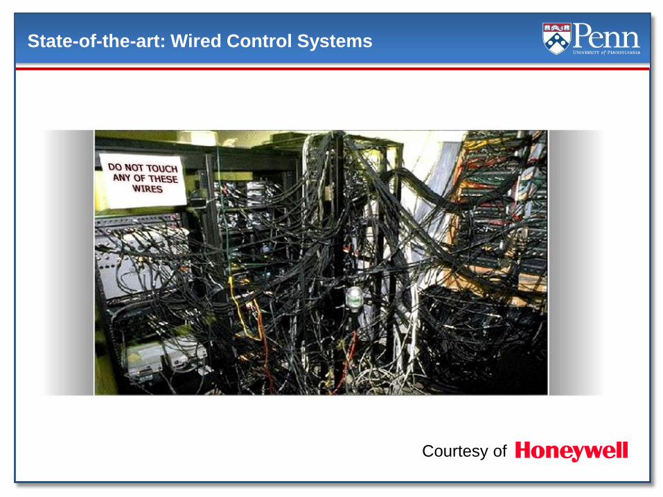
State-of-the-art: Wired Control Systems
Courtesy of

Challenges with Wired Control Systems
• Wires are expensive – Wires as well as installation costs
– Wire/connector wear and tear
• Lack of flexibility – Wires constrain sensor/actuator mobility
– Limited reconfiguration options
• Restricted control architectures – Centralized control paradigm
Plant Controller

The promise: Wireless Control Systems
Courtesy of

The promise: Wireless Control Systems
Courtesy of
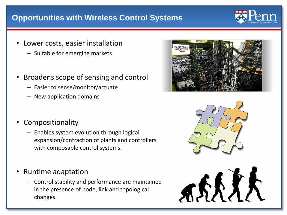
Opportunities with Wireless Control Systems
• Lower costs, easier installation – Suitable for emerging markets
• Broadens scope of sensing and control – Easier to sense/monitor/actuate
– New application domains
• Compositionality – Enables system evolution through logical
expansion/contraction of plants and controllers with composable control systems.
• Runtime adaptation – Control stability and performance are maintained
in the presence of node, link and topological changes.

Wireless is transformative for industrial control
• Paradigm shift towards wireless control architectures
• Single-hop and multi-hop communication networks
Wired Control System Wireless Control System
Plant Controller
Plant Controller

Control over wireless communication networks
Plant Controller Controller Plant
Channel
Channel
• General challenges include network-induced delay, single-packet vs. multi-packet transmission systems, dropping of communication packets
• Single-hop vs multi-hop networks
Abstracts away system design
• Standard Wireless Control Systems employ packet routing to deliver information to centralized controllers
• Control performance depends on the network’s QoS

Wireless is transformative for industrial control
• Paradigm shift towards multi-hop control architectures
Wired Control System Wireless Control System
Plant Controller
Plant Controller
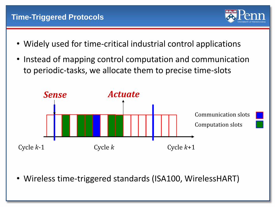
Time-Triggered Protocols
• Widely used for time-critical industrial control applications
• Instead of mapping control computation and communication to periodic-tasks, we allocate them to precise time-slots
• Wireless time-triggered standards (ISA100, WirelessHART)
Communication slots
Computation slots
Sense Actuate
Cycle k-1 Cycle k Cycle k+1

WirelessHART
• TTA Architecture (TDMA – FDMA), 10ms slots
• 10

Wireless Control Systems: Technical Challenges
• Modeling – Holistic modeling of control, communication, computation
– Interfaces between control and time-triggered communication
• Analysis – Impact of TDMA-based wireless on control performance
– Compositional scheduling of multiple control loops
• Synthesis – Control-scheduling co-design
– Controller design incorporating TDMA-based properties
– Network topology design based on physical plant properties
• Robustness – Robustness analysis with respect to packet loses, node failures
– Robustness with respect to faulty or malicious nodes

Outline
• Optimal Power Management in Wireless Control Systems
– Power-aware control over single-link networks
• Control with multi-hop wireless networks
– Routing-based control over time-triggered networks
• Wireless Control Networks
– A simple decentralized approach for in-network control
Plant
Sensor Actuator
Plant Controller
Plant
WCN


Optimal Power Management in Wireless Control Systems
• Optimal Power Management in Wireless Control Systems*
– Control over a single wireless link
– Separation & optimal plant control
– Optimal and suboptimal communication policies
*K. Gatsis, M. Pajic, A. Ribeiro, and G.J. Pappas. Power-aware communication for wireless
sensor-actuator systems, IEEE Conference on Decision and Control, submitted.
K. Gatsis, A. Ribeiro, G.J. Pappas, Optimal power management in wireless control
systems, American Control Conference, 2013.
K. Gatsis, A. Ribeiro, G.J. Pappas, Optimal power management in wireless control
systems. IEEE Transactions on Automatic Control, submitted
Plant
Sensor Actuator

Motivation: Managing Power Resources
• Control systems with power-constrained wireless sensors, e.g. HVAC, building/industry automation
• Power regulation: sensor lifetime
• Impact & trade-offs with closed-loop control task

Challenges of Power Management in Wireless Control
• Common mathematical framework for control/wireless communications
- unpredictable wireless conditions
- online power adaptation (PHY layer)
- timely & reliable information delivery
- controller design
• Methodology for (co-) design power & plant control mechanisms
• Advantages & new insights – in contrast to “control-only” or “communication-only” perspectives
Communications
Control

Literature: Control under Communication Constraints
• Communication as a constraint/disturbance
- Estimation and Control under packet drops [Hespanha et al 2007], [Sinopoli et al 2004], [Schenato et al 2007], [Gupta et al 2007], [Imer et al 2006]
- Communication as model uncertainty (robust control techniques) [Elia 2005], [Braslavsky et al 2007]
Communication not part of the design

Literature: Communication & Control
• Communication with data-rate constraints: coding & control design
- [Tatikonda, Mitter 2004], [Nair et al 2007], including power [Quevedo et al 2010]
Communication design: encoding & bit-rate for stability
• Event-based paradigm: sensor (actuator) decides whether to transmit (actuate) or not
- Estimation [Xu, Hespanha 2004], [Cogill et al 2007], [Mesquita et al 2012], [Li, Lemmon 2011]
- Control [Tabuada 2007], [Anta, Tabuada 2010], [Rabi, Johansson 2009], [Molin, Hirche 2009], [Donkers et al 2011]
Communication cost: average number of transmissions

• Single loop with power-constrained sensor/transmitter & power-free receiver/actuator
• Goal: design power control & plant control mechanisms
• On-line by adapting to both wireless channel conditions and plant state
- Less power when plant ‘close’ to stability
- Good channel - cheap to transmit vs. bad channel - costly
Power-aware Control over Wireless
Plant
Sensor Actuator

Wireless Control Architecture
• Channel state information hk available at transmitter
• Power adaptation pk to both channel hk & plant xk
• Packet drops capture both effects of random wireless channel
& protection by power

Wireless Control Architecture & Co-design
Decision variables
• Performance: Joint average linear quadratic and power costs

Wireless Communication Model Decoding depends on power and channel
• Received signal-to-noise ratio
• Probability of successful decoding
• Combine in qk = q(hk , pk)
-
- hk block fading, i.i.d.
- N0 : AWGN power level
- determined experimentally - depends on error-correcting code

Novelties of our Wireless Control Architecture
• Generalizes standard Bernoulli packet drops
Wireless effects are explicitly captured
Bernoulli successes are actively controlled by power
• Generalizes event-triggered transmissions
Decision depends also on wireless conditions
Communication cost is power consumption vs. transmission rate
• Packet-based communication: unlike data-rate constraints & coding

Joint Optimal Communication & Control
• Information structure couples decisions:
Control action uk affects power decision pk+1 through xk+1

Restricted Information Structure
• Controller keeps estimate*
• Innovation terms at sensor/transmitter (known by ACK):
• Restrict available information: innovation and channel
• Control input does not affect transmitter - no effect on quality of future plant state estimation
* Optimal if information from lost packets is removed

• Adapt power to innovation and channel
Separation & Optimal Plant Control

Conditions for Optimal Control Theorem
• Assumptions: (A,B) controllable, (A, Q1/2) observable, and
for every channel h *
- relates to stability of the jump estimation errors when transmitter uses full power
- guarantees that for any
there exists a finite uniform bound
* Can be relaxed – in expectation over h

Proof of Optimal Control Theorem
• Finite horizon N - standard LQR Bellman equation & solution
since plant input has no effect on future plant estimates, and
with standard Riccati recursion
• Limit of finite horizon optimal cost
Converge by controllability/ observability assumptions

Optimal Communication Policy
• Optimal communication: estimation vs. power
- Reduces to a Markov Decision Process: state , action p
- Existence of solution to Bellman equation is shown
- Not computationally tractable due to continuous state space

Characterization of Optimal Communication Policy
• Optimal power allocation in terms of an unknown penalty on innovation
• Zero power when error small or channel fading low
• Area depends on weight λ • Outside zero-power region adapt power to both plant and channel • “Soft” event-triggering

Characterization of Optimal Communication Policy Dependence on error-correcting code
• Effect of different error-correcting codes
• Fixed channel h
• Zero-power region depends on shape of function q(h,p)
• “Soft” event-triggering: power adapts to plant when transmitting

Theoretical Limit for Capacity Achieving Codes
• Model capacity achieving
codes by indicator
• Optimal (not tractable)
- Packet success qk = 0 or 1
Recover standard event-triggered transmit-or-not policies,
trigger depends on channel and estimation error!

Rollout policy (model predictive):
“optimize current power as if future policy is some reference”
- Reference policy adapting only to channel p(h)
- Bernoulli packet success
- Quadratic cost-to-go
Suboptimal Communication Policies
Approximates optimal

Simulation of Suboptimal Policies – General Codes
• Quadratic penalty on error
• Characteristics similar to the optimal policy

Simulation of Suboptimal Policies – Capacity Achieving
Blue: don’t transmit, Red: transmit
• Policies become event-triggered • Rollout policy adapts to plant structure

Summary of Results
• Richer communication model:
captures uncertainties of wireless & power adaptation
• Communication/control separation can be established (suboptimal but otherwise joint cost hard to analyze)
• Optimal communication is ‘soft’ event-triggered
zero power if error small or channel adverse
power adaptation to both plant and channel states otherwise
• Communication policies can be designed by ADP techniques

A New Paradigm for Control / Wireless Networking
• Model, analysis, communication/control co-design of complex wireless sensor & actuator networks
- Multiple or distributed plants
- Shared wireless channels (interference)
- Optimal control-aware resource allocation, e.g. power, scheduling
- Economic resource-aware controller synthesis

Limitation: Not Power-aware at Receiver
• Architecture limitation:
- wireless receiver/controller always listens
- comparable power consumption at both ends
- common in any event-based scheme over wireless
Plant
Sensor Actuator

Power-aware Wireless Receiver Design
• Ideally: Turn off receiver between transmissions…
inconsistent with event-triggering
• Our approach: coordination protocol
Devices turn off and agree on next wake-up time (self-triggered* step)
Upon wake-up sensor decides whether to transmit or not (event-triggered step)
How to ‘predict’ when next event will occur?
Consider power costs at both ends, current channel & plant states
*[Anta, Tabuada 2010]
Event-based Low Transmission
Rate
Receiver
Under-utilized

Simplified Problem Setup
• Markov fading channel (finite states, irreducible, aperiodic)
- possibility of predicting good channels
• Capacity achieving code
• Constant power penalty pa for awake receiver, pk for transmitter as before
• Fixed LQR controller
• Trade-off estimation error vs. power at both ends

Optimal Self-triggered Protocol
• Self-triggered protocol:
Cost independent of plant state : estimation error is reset on every transmission
Sleep-time need only depend on channel state : predict when channel suitable and estimation error not too large
Optimal computed by analogy to a MDP (tractable for finite channel states)

Proposed Protocol Improvement to optimal self-triggered
• Proposed protocol – model predictive
Upon wake-up decide whether to transmit & sleep according to optimal self-triggered, or skip current step
Current decision based on modeling future behavior & cost
Guaranteed to perform not worse than optimal self-triggered
Injects event-triggered steps between sleep

Protocol Performance Comparison
• Ratio of proposed protocol / optimal self-triggered as receiver’s constant power increases
If power for receiver to stay awake dominates power for transmitter to communicate, self-triggered performs best

Summary & Future Work
• New Paradigm for Control/ Wireless Networking
- Model capturing explicitly wireless fading channel effects and power allocation & interaction with control task
- Novel Physical Layer design: Characterization of optimal power adaptation to channel & plant conditions
- Receiver power considerations via a coordination protocol
• Future work
- Medium Access Control for multiple closed-loops over a shared wireless channel
- Control-aware Resource Allocation, e.g. scheduling, power, in wireless networked control systems

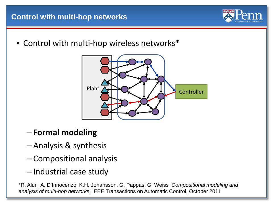
Control with multi-hop networks
• Control with multi-hop wireless networks*
– Formal modeling
– Analysis & synthesis
– Compositional analysis
– Industrial case study
Plant Controller
*R. Alur, A. D’Innocenzo, K.H. Johansson, G. Pappas, G. Weiss Compositional modeling and
analysis of multi-hop networks, IEEE Transactions on Automatic Control, October 2011

Control with multi-hop networks: Modeling
• A multi-hop wireless networked system
• Assumptions:
– Plants/controllers are discrete-time linear systems
– Multi-hop network runs time-triggered protocol

Control with multi-hop networks: Modeling
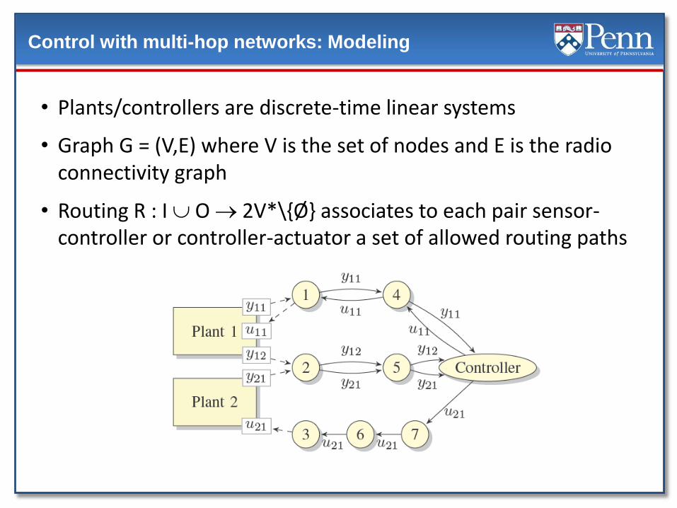
• Plants/controllers are discrete-time linear systems
• Controllers are designed to achieve suitable performance

Control with multi-hop networks: Modeling
• Plants/controllers are discrete-time linear systems
• Graph G = (V,E) where V is the set of nodes and E is the radio connectivity graph
Control with multi-hop networks: Modeling
• Plants/controllers are discrete-time linear systems
• Graph G = (V,E) where V is the set of nodes and E is the radio connectivity graph
• Routing R : I O 2V*\{Ø} associates to each pair sensor-controller or controller-actuator a set of allowed routing paths

Communication and computation schedule

Evolution in each time step

Integrated modeling
Given communication and computation schedules, the closed loop multi-hop control system is a switched linear system
where the schedule (discrete switching signal) is either:
1. Deterministic and periodic
2. Nondeterministic and periodic
3. Stochastic due to packet loss, failures
Modeling the multi-hop control network as a hybrid system!

Control with multi-hop networks
• Control with multi-hop wireless networks
– Formal modeling
– Analysis & synthesis
– Compositional analysis
– Industrial case study
Plant Controller

Analysis of multi-hop control networks
• Periodic deterministic schedule (static routing, no TX errors):
– Theory of periodic time varying linear systems applies
– Schedule is a fixed string in the alphabet of edges/controllers
– Nghiem, Pappas, Girard,Alur – EMSOFT 2006, ACM TECS 2012
• Periodic non-deterministic schedule (dynamic routing):
– Theory of switched/hybrid linear system can be applied
– Schedule is an automaton over edges/controllers
– Alur, Weiss – HSCC 2007
• Stochastic analysis (stochastic packet loss, failures):
– Theory of discrete time Markov jump linear systems applies
– Schedule is a Markov Chain over edges/controllers
– Alur, D’Innocenzo, K.H. Johannsson, Pappas, Weiss, IEEE CDC 2009, IEEE TAC 2011

Periodic deterministic schedules
+
-
Ideal
Control
Multi-hop
Wireless
Control
Error can be
computed exactly*
*T. Nghiem, G. Pappas, A. Girard, R. Alur, Time triggered implementations of dynamic
controllers, ACM Transactions on Embedded Computing Systems, 2012, In press

Modeling communication failures
We consider 3 types of failure models:
Long communication disruptions (w.r.t the speed of the control system)
Permanent link failures
Typical packet transmission errors (errors with short time span)
Independent Bernoulli Failures
A general failure model where errors have random time span
A Markov model

Permanent link failures
Decision problem: Given a permanent failure model, determine if
where Pstable - probability that the multi-hop control is stable.
Permanent failure decision problem is NP-hard (CDC 2009)
Works for small networks/control loops
Pstable ³a
Permanent failures are modeled by a function F : E [0,1]
F(v1, v2) models the probability that the link (v1,v2) fails.

Control with multi-hop networks
• Control with multi-hop wireless networks
– Formal modeling
– Analysis & synthesis
– Compositional analysis
– Industrial case study
Plant Controller

Interfaces for compositional control
Control Design
Sampling frequency
Delays, jitter
Scheduling
WCET
RM, EDF
Problems
Impact of scheduling on control
Composing schedules

Interfaces for compositional control*
Control Design
Control loop must get
at least one slot in a
superframe of 4 slots
Scheduling
Non-deterministic schedules
for time-triggered platforms
0
0
0
1 1 1
1
*R. Alur and G. Weiss, Automata-based interfaces for control and scheduling, HSCC 2007

Control specifications as automata
• Stability Control Specifications
• Periodic Control Specifications on TTA
• Timing Constraints:
Automata specifying schedules that guarantee stability
Sample every 100 seconds
If not sampled in the last 200 seconds, sample every 10 seconds for the next minute
Specifications of maximal time delays between events
Automata that specify valid periodic schedules
Specifications of maximal time delays between events

LQR over TTA architectures*
• Consider control plant with resource constraints on actuator
• Time-dependent switching signal allows only one actuator active at any time
• Many related approaches by Hristu/Brockett ‘95, Lincoln and Bernhandnsson 2000, Zhang, Hu, Abate 2010 etc.
• Generally discrete-time, computationally intensive search for switching signal.
*J. Le Ny, E. Feron, and G. J. Pappas, Resource constrained LQR control under fast sampling, HSCC 2011

LQR over TTA architectures
• Minimize steady state LQR cost over control input and switching signal
• Subject to constraints

Key technical ideas
• Given switching signal and T, LQR controller is optimal. Hence
• Optimize above cost over steady-state average utilizations per input
• We are keeping average utilization but we are ignoring order
• Subject to switching signal allows only one actuator active at any time

Performance bounds over average utilization
• Compute performance bound using semi-definite programming
• Optimize above cost over steady-state average utilizations per input
• Theorem (HSCC 2011): In the limit of arbitrarily fast switching , these policies are asymptotically optimal.
• Subject to switching signal allows only one actuator active at any time

• For simple system with three inputs, SDP provides optimal utilization rates
• Approximate optimal utilization rates
• In a schedule of 100 slots, 54 slots go to input 1, 44 to input 2, etc
• Tradeoff between length of schedule and approximation of utilization
• Subject to switching signal allows only one actuator active at any time
Time-triggered approximations to LQR

Sample system realizations (10ms slots)

Control specifications as automata
• Stability Control Specifications
• Periodic Control Specifications on TT
• Timing Constraints:
Automata specifying schedules that guarantee performance
Sample every 100 seconds
If not sampled in the last 200 seconds, sample every 10 seconds for the next minute
Specifications of maximal time delays between events
Automata that specify valid periodic schedules
Specifications of maximal time delays between events

Automata are compositional
0
0
0
1 1 1
1 0
0
0
1 1 1
1
∩ = ?

Price of composability
• The more robust the controller, the larger the automaton that can be tolerated with acceptable performance loss.
• The larger the automaton that can tolerated, the more composable our limited resources will be.
• Tradeoff between control performance and composability
• Timing Constraints:

Control with multi-hop networks
• Control with multi-hop wireless networks
– Formal modeling
– Analysis & synthesis
– Compositional analysis
– Industrial case study
Plant Controller

Mining Industry Case Study
• Mining phases:
– Drilling and blasting
– Ore transportation
– Ore concentration
Boliden mine in Garpenberg, Sweden

Floatation bank control problem
H. Lindvall, “Flotation modelling at the Garpenberg concentrator using Modelica/Dymola,”, 2007.

Process Time Scales: Zn Flotation
Loop category
# of loops in category
Loop name Sampling interval (Ts)
Air flow 9 FA301_FC1 2
FA302_FC1 2
FA303_FC1 2
FA304_FC1 2
FA305_FC1 2
FA101_FC1 2
FA102_FC1 2
FA103_FC1 2
FA104_FC1 2
Level 6 FA302_LC1 2
FA303_LC1 1
FA305_LC1 8
FA102_LC1 8
FA103_LC1 8
FA104_LC1 8
Loop category
# of loops in category
Loop name Sampling interval (Ts)
Reagents 2 BL031_FC1 2
FA300_FC2 1
• Each controlled variable represents a control loop
• Only the main control loops: • air flow, pulp level and reagent
• Each loop abstracted by a time constraint (the sampling interval)
• specifies the maximum delay between sensing and actuation
• The sampling interval used as a constraint for defining the set of “good” schedules

Wireless network topology

Using SMV to compose schedules
MODULE loop2(bus)
VAR
cnt:0..6;
ASSIGN
init(cnt):=0;
next(cnt):=case
bus=e2to5 & cnt=0 : 1;
bus=e5toc & cnt=1 : 2;
bus=bus & cnt=2 : 3;
bus=ecto7 & cnt=3 : 4;
bus=e7to6 & cnt=4 : 5;
bus=e6to3 & cnt=5 : 6;
1:cnt;
esac;
DEFINE
done := cnt=6;
MODULE loop1(bus)
VAR
in1:0..2;
in2:0..2;
out1:0..3;
ASSIGN
init(in1):=0;
init(in2):=0;
init(out1):=0;
next(in1):=case
bus=e1to4 & in1=0 : 1;
bus=e4toc & in1=1 : 2;
1:in1;
esac;
next(in2):=case
bus=e2to5 & in2=0 : 1;
bus=e5toc & in2=1 : 2;
1:in2;
esac;
next(out1):=case
bus=bus & allin & out1= 0 :1;
bus=ecto4 & allin & out1= 1 : 2;
bus=e4to1 & allin & out1= 2 : 3;
1 : out1;
esac;
DEFINE
allin := in1=2 & in2=2;
done := out1=3;
MODULE main
VAR
bus:{e1to4, e2to5, e4to1, e4toc, e5toc, e6to3, e7to6, ecto4, ecto7, idle};
l1:loop1(bus);
l2:loop2(bus);
SPEC
AG !(l1.done & l2.done);
Req. For Plant 2:
e2to5, e5toC, …,e6to3
must be a subsequence
of the schedule
We are looking for a schedule that
satisfies both requirements which
comes as a counter-example to the
claim that there is no such schedule
progress
counters
Req. For Plant 1:
more involved because it
has two inputs

Case study results
17 single-input-single-output loops Timing constraints At most one message in a time slot
SMV code with 18 modules 272 lines BDD nodes allocated: 26797
Shortest schedule that satisfy the constraints posed by all 17 loops 37 time slots
~2 minutes

Future challenges
• Time-triggered architectures not optimal for event-based systems
– Hybrid TDMA/CSMA or LTTA architectures
– Event-based sensing and control
• Time-synchronization for large networks
– Model TDMA clock drift using timed automata
– Scheduling by composing timed-automata
• Wireless models are not precise
– On-line adaptation of packet drop probability
– Robust/adaptive control
• Control over virtual network computation
– Runtime control reconfiguration in presence of node failures
– Embedded virtual machines for control [Pajic, Mangharam 2012]
Plant


The Wireless Control Network (WCN)
• In multi-hop control, nodes route information to controller
• Can we leverage computation of the network?
• Can we distribute the controller to nodes of the network?
• Reminiscent of network coding
Plant Controller Plant
WCN
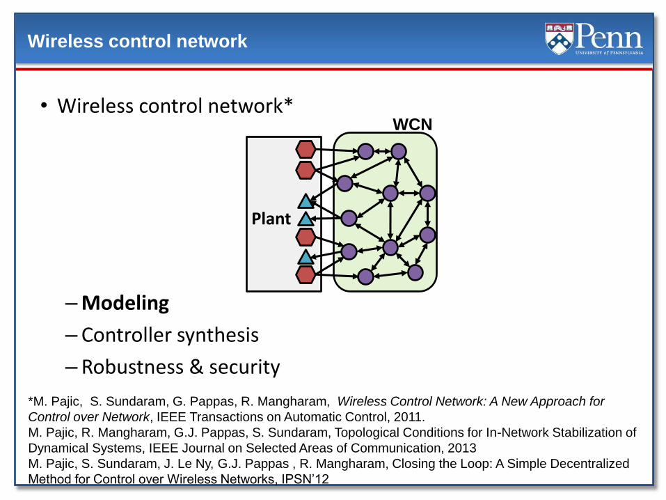
Wireless control network
• Wireless control network*
– Modeling
– Controller synthesis
– Robustness & security
Plant
WCN
*M. Pajic, S. Sundaram, G. Pappas, R. Mangharam, Wireless Control Network: A New Approach for
Control over Network, IEEE Transactions on Automatic Control, 2011.
M. Pajic, R. Mangharam, G.J. Pappas, S. Sundaram, Topological Conditions for In-Network Stabilization of
Dynamical Systems, IEEE Journal on Selected Areas of Communication, 2013
M. Pajic, S. Sundaram, J. Le Ny, G.J. Pappas , R. Mangharam, Closing the Loop: A Simple Decentralized
Method for Control over Wireless Networks, IPSN’12

Distributed control over time-triggered network
• Each node maintains its (possible vector) state – Transmits state exactly once in each step (per frame)
– Updates own state using linear iterative strategy
• Example:
v6
v8
v5
v4 v3
v2
z5 = 1
z2 = 2
z3 = -2
z8 = 3.2
z6 = -4.3
z4 = 0.2
Slot 1: v4 transmits
v6
v8
v5
v4 v3
v2
z5 = 1
z2 = 2
z3 = -2
z8 = 3.2
z6 = -4.3
z4 = 0.2
Slot 2: v5 transmits
v6
v8
v5
v4 v3
v2
z5 = 1
z2 = 2
z3 = -2
z8 = 3.2
z6 = -4.3
z4 = 0.2
Slot 3: v2 transmits
v6
v8
v5
v4 v3
v2
z5 = 1
z2 = 2
z3 = -2
z8 = 3.2
z6 = -4.3
z4 = 0.2
Slot 4: v8 transmits
v6
v8
v5
v4 v3
v2
z5 = 1
z2 = 2
z3 = -2
z8 = 3.2
z6 = -4.3
z4 = 0.2
Slot 5: v6 transmits
v6
v8
v5
v4 v3
v2
z5 = 1
z2 = 2
z3 = -2
z8 = 3.2
z6 = -4.3
z4 = 0.2
Slot 6: v3 transmits
4 2 6 8 5 3
Transmit slots
v4 informed about its neighbors states
v4 updates its state

WCN modeling
• Discrete-time plant
• Node state update procedure:
• Actuator update procedure:
From neighbors From sensors
From actuator’s neighbors Plant
WCN

WCN modeling
• Network acts as a linear dynamical compensator
Structural constraints: Only elements corresponding to existing links (link weights) are allowed to be non-zero
Plant
WCN

WCN modeling: Closing the loop
• Overall system state:
• Closed-loop system:
• Matrices W, G, H are structured
• Sparsity constraints imposed by topology!
plant
network
Plant
WCN

WCN Advantages: Simple & Powerful
• Low overheard
– Each node only calculates linear combination of its states and state of its neighbors
– Suitable even for resource constrained nodes
– Easily incorporated into existing wireless networks (e.g., systems based on the ISA100.11a or wirelessHART)
– Backup mechanism in ‘traditional’ networked control systems; used for graceful degradation

WCN Advantages: Scheduling
• Simple scheduling
– Each node needs to transmit only once per frame
– Static (conflict-free) schedule
• No routing!
• Multiple sensing/actuation points
– Geographically distributed sensors/actuators
Building automation
Process control

WCN Advantages: Compositionality
• Adding new control loops is easy!
– Does not require any communication schedule recalculation
• WCN configurations can be combined
Stable configuration
Plant2
Plantk
…
Plant1
Fixed in
animation

Wireless control network
• Wireless control network
– Modeling
– Controller synthesis
– Robustness & security
Plant
WCN

WCN controller synthesis
• Use WCN to stabilize the closed-loop system
– Synthesis of optimal WCN configurations
• Does the plant influence the WCN network topology?
– How many nodes? How to interconnect them?
• Given network topology, design distributed controller
– Extracting a stabilizing closed loop configuration
Plant

Topological conditions for stabilization vs. information
transmissions
• The objective of the network is systems stabilization!
• Example:
• This network is not capable of delivering all of the source information to all of the sinks at each time-step
• That is not necessarily a cause for concern when the main objective is to stabilize the system.

WCN topological conditions
• Structured system theory: Systems represented as graphs
• Linear system
• Associated graph H
• Properties of graph are generic properties of structured system
1 2 7
3 4 5
8
6
0 0 0
0 0 0[ 1] [ ] [ ],
0 0 0 0 0
0 0 0 0 0
x k x k u k
][
000
000
000
][
11
10
9
kxky
1
2
4 3 Output vertices: Y
State vertices: X
Input vertices: U

A small detour into decentralized control…
Plant
Controller 1
Controller 2
Controller m
…
Actuators
Decentralized control system
From feedback patterns
Fixed Modes [Wang & Davison, 1973; Siljak, 1981]
Indicate whether the system can be stabilized

New closed-loop system model
The plant ↔ network model
New plant: Plant & WCN
Controlled by controllers at the actuators
Plant
WCN

• Use structured system theory and decentralized control on the WCN and network
• Can we stabilize the plant with 2 nodes?
WCN topological conditions
][
5
4
6.1
1
2
5.0
1
0
][
3000
0200
41020
3102
]1[ kukxkx
][101.00
023.01][ kxky
z2 z1
x3
x1
x2
u1
y1
Plant
WCN
u2
y2x4

Topological Conditions for WCN
• Consider a numerically specified system
• Example: A system with integrators
Network condition: Let d denote the largest geometric multiplicity of any unstable eigenvalue of the plant. If
1) connectivity of the network is at least d, and
2) each actuator has at least d nodes in neighborhood
then there exists a stabilizing configuration for WCN
Eigenvalues are 2,2,2,3
Λ=2 has geometric multiplicity d=2 (≥ 1)
3000
0200
41020
3102
A

• Use structured system theory on WCN and network
• We cannot stabilize with with 2 nodes!
WCN topological conditions
][
5
4
6.1
1
2
5.0
1
0
][
3000
0200
41020
3102
]1[ kukxkx
][101.00
023.01][ kxky
z1
z2
s1
a1
a2
s2
Plant
WCN

• Use structured system theory on WCN and network
• We cannot stabilize with with 2 nodes!
• But we can stabilize plant with 4 nodes
WCN topological conditions
][
5
4
6.1
1
2
5.0
1
0
][
3000
0200
41020
3102
]1[ kukxkx
][101.00
023.01][ kxky
z1
z2
s1
a1
a2
s2
Plant
WCN
z4
z3

WCN topological conditions
• Is fully connected network sufficient?
Sufficient condition: If
1) Geometric multiplicity is 1 for all unstable eigenvalues,
2) System is controllable and and observable,
then it can be stabilized with a strongly connected network, where each sensor and actuator is connected to the network.
Generic condition!

Topological conditions for point-to-point networks
• Problem: network synthesis for stabilization when network coding over point-to-point communication links is used
• Example: Point to point communication in a simple network
• Algebraic approach to network coding (Koetter, Medard, 2005) – each link in the initial graph is mapped to a unique vertex in the line graph
• The labeled line graph directly corresponds to the WCN model!
• This network is not capable of delivering all of the source
information to all of the sinks at each time-step
• That is not necessarily a cause for concern when the main objective is to stabilize the system.
Direct labeled line graph

Topological conditions for point-to-point networks
• Consequently, the same reasoning can be used for point-to-point networks
Sufficient condition when point-to-point networks with linear network coding are used for communication:
Let d denote the largest geometric multiplicity of any unstable e-value of a detectable and stabilizable plant. If edge connectivity of the network between sensors and actuators is at least d then the system can be stabilized using dynamic compensators at actuators.
The equivalent generic condition also holds!

Topological conditions for point-to-point networks
• Problem: network synthesis for stabilization, in the case where network coding over point-to-point communication links is used
• Examples: Point-to-point communication in simple networks
Stabilizable for d≤3 Stabilizable for d≤1

WCN controller synthesis
• Use WCN to stabilize the closed-loop system
• For a specific WCN network topology
– How to stabilize the closed-loop system
Plant
WCN

Stabilizing the Closed-Loop System
• Problem: Find numerical matrices W, H, G satisfying structural constraints such that
• Solution: Formulate Lyapunov function and try to solve using Linear Matrix Inequalities (LMIs)
— Find positive definite matrix P such that
ˆ
A BGA
HC Wis stable
ˆ ˆ 0T P A PA
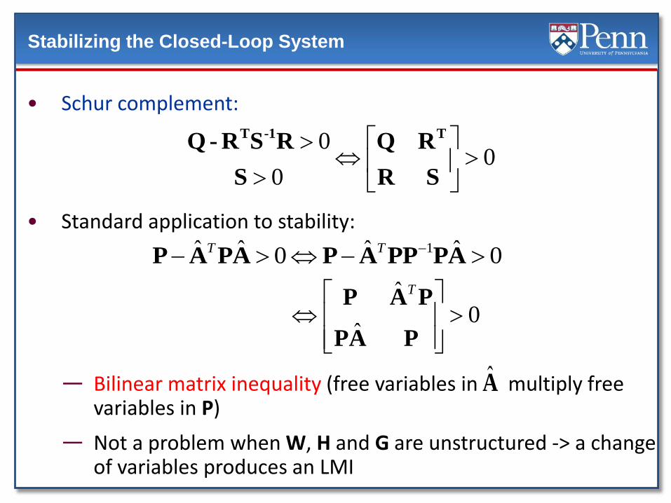
Stabilizing the Closed-Loop System
• Schur complement:
• Standard application to stability:
— Bilinear matrix inequality (free variables in multiply free variables in P)
— Not a problem when W, H and G are unstructured -> a change of variables produces an LMI
00
0
T -1 TQ- R S R Q R
S R S
1ˆ ˆ ˆ ˆ0 0T T P A PA P A PP PA
ˆ0
ˆ
T
P A P
PA P
A

Stabilizing the Closed-Loop System
• Change of variables no longer works when is structured
• Alternative approach [de Oliveira et. al, CDC’00]:
• Problem is still nonconvex,
— This form appears frequently in design of static output feedback controllers
A
1
ˆˆ ˆ 0 0
ˆ
T
T
P AP A PA
A P
ˆ0,
ˆ
T
P AQP I
A Q
linear in A
nonconvex constraint

Stabilizing the Closed-Loop System
• Various methods developed to deal with constraint QP = I
• Use approach by [El Ghaoui et al., TAC, 1997]:
— Positive definite nxn matrices P and Q satisfy QP = I if and only if they are optimal solutions to the problem
and the minimum cost is n.
• Still nonlinear -> linearize around a feasible point P0, Q0
min ( )
. . 0
tr
s t
QP
P I
I Q

Convex relaxation for controller synthesis
1 1
1 1 1
11 1
1
1
1 1
1 1 1 1 1
min ( )
ˆ0, 0,
ˆ
ˆ ,
( , , ) , 0, 0
k k k k
T
k k k
kk k
k
k
k k
k k k k k
tr
P Q Q P
P A P I
I QA Q
A BGA
H C W
W H G P Q
Find feasible points P0, Q0, W0, H0, G0
Solve the LMI problem, from Pk, Qk find
Pk+1, Qk+1, Wk+1, Hk+1, Gk+1
System stable
Configure WCN
yes
no
Function Linearization

Synthesis of optimal WCNs
Goal: A WCN configuration that minimizes the impact of disturbances!
• Model as a new system:
where the goal is to minimize .
Disturbance impact
closed-loop: WCN & plant!

Synthesis of optimal WCNs
How to capture size of discrete time signals?
System gains for the discrete-time system
• Energy-to-Peak Gain:
• Energy-to-Energy Gain:
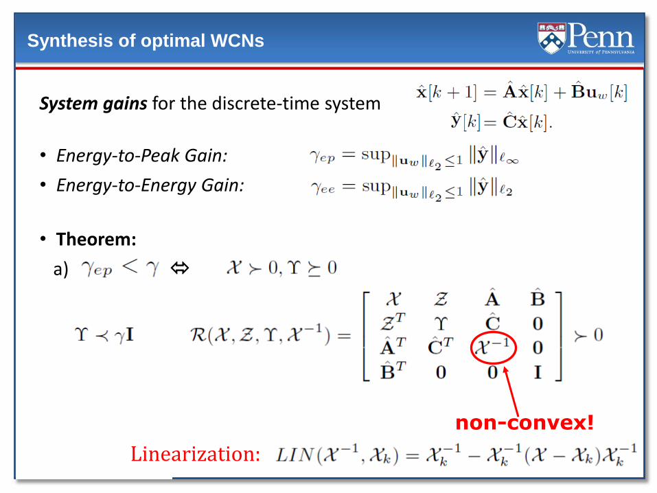
Synthesis of optimal WCNs
System gains for the discrete-time system
• Energy-to-Peak Gain:
• Energy-to-Energy Gain:
• Theorem:
a)
non-convex!
Linearization:

Convex relaxation for controller synthesis
Find feasible points X0, Z0, W0, H0, G0
Solve the LMI problem, from Xk find
Xk+1, γk+1, Wk+1, Hk+1, Gk+1
Configure WCN
yes
no
Function Linearization
For ,

WCN Synthesis
Network Synthesis
WCN Configuration
Plant Dynamics
Stabilizing WCN Configuration
Network Topology
The plant influences the network design!

Wireless control network
• Wireless control network
– Modeling
– Controller synthesis
– Robustness & security
Plant
WCN

WCN robustness to link failures
• What happens if links in the network fail?
– Bernoulli distribution: fails with some probability
• Many links in network: how to model concisely?
– Use robust control [Elia, Sys & Control Letters, ‘05]
– Received value: ji[k]zi[k] = ( + ji[k])zi[k]
ziξji
ξjizivi vjxwji
vjvizi μ
Δjiri
x
wji
+
Mean (fixed) part
Variance
(random) part
Link modeled as
random process
mean (constant)
random variable
zero-mean random variable

System Model with Link Failures
][xJ]r[ or kk
• Closed loop system with uncertainties:
ˆ ˆ[ 1] [ ]k k
A BGx x
HC Wnominal (mean) system
uncertainties r[k]
Mean (fixed) part Random part
ˆ ˆ[ 1] [ ] [ ] [ ]k k k k
A BGx x J r
H C W

• Closed loop system with random Bernoulli failures
System is mean square stable if and only if there exists X, α1,α2,…,αN such that
• Robustness requires – One additional constraint added for each link (Bernoulli failures)
– More constraints for more general failure models
– Significant improvements with observer style updates
WCN robustness to link failures
ˆ ˆ[ 1] [ ] [ ] [ ]k k k k
A BGx x J r
H C W

Robustness to Link Failures
• Example
For α=2, maximal message drop probability which guarantees MSS
pmax ≤ 1.18% << 25%
How can we improve robustness of the WCN to link failures?
w21
v1
x[k+1]=αx[k]+u[k],
y[k]=x[k]
v2
y[k]u[k]
w12
g h

Problem: How to improve robustness to link failures?
• Idea: Include observer style updates
– different weights depending of the success of the transmission
Observer Style Updates – for reliable communication links
Standard observer
A similar design-time iterative algorithm can be used to extract robust WCN configurations!

Robustness to Link Failures - Evaluation
w21
v1
x[k+1]=αx[k]+u[k],
y[k]=x[k]
v2
y[k]u[k]
w12
g h
• Example
• Maximal message drop probability which guarantees MSS, α=2

Robustness to Link Failures - Evaluation
w21
v1
x[k+1]=αx[k]+u[k],
y[k]=x[k]
v2
y[k]u[k]
w12
g h
• Example
• Maximal message drop probability which guarantees MSS, α=2

Robustness to Link Failures - Evaluation
w21
v1
x[k+1]=αx[k]+u[k],
y[k]=x[k]
v2
y[k]u[k]
w12
g h
• Example
• Maximal message drop probability which guarantees MSS, α=2

Robustness to Link Failures
• Example – WCN with observer style updates
For α=2, maximal message drop probability which guarantees MSS
pmax ≈ 21% < 25%
Approaching theoretical limit for robustness with centralized controllers!
w21
v1
x[k+1]=αx[k]+u[k],
y[k]=x[k]
v2
y[k]u[k]
w12
g h

Monitoring for faulty and malicious behavior
• What if certain nodes in the WCN become faulty or malicious?
• Security of control networks in industrial control systems is a major issue [NIST Technical Report, 2008] – Data Historian: Maintain and analyze logs of plant and network behavior
– Intrusion Detection System: Detect and identify any abnormal activities
• Is it possible to design an Intrusion Detection System to determine if any nodes are not following WCN protocol?
• Can IDS scheme avoid listening all nodes? Under what conditions? Which nodes?

IDS for wireless control network
• Consider graph of wireless control network with plant sensors
• Denote transmissions of any set T of monitored nodes by
– T is a matrix with a single 1 in each row, indicating which nodes z[k] are being monitored
Plant
WCN y[k]
u[k]
source node (plant sensor)
[ ] [ ]k kt Tz

Modeling with malicious nodes
• WCN model with set S of faulty/malicious nodes:
• Objective: Recover y[k], fs[k] and S (initial state z[0] known)
– Almost equivalent to invertibility of system
• Problem: Don’t know the set of faulty nodes S
– Assumption: At most b faulty/malicious nodes
• Approach: Must ensure that output sequence cannot be generated by a different y[k] and possibly different set of b malicious nodes
[ 1] [ ] [ ] [ ]
[ ] [ ]
S Sk k k k
k k
z Wz Hy B f
t Tz

Conditions for IDS Design
IDS can recover y[k]
and identify up to b
faulty nodes in the
network by monitoring
transmissions of set T
Can recover inputs and set S in system
for any unknown set S of b nodes
Linear system
is invertible for
any known set Q of 2b nodes
There are p+2b
node-disjoint paths
from sensors and any
set Q of 2b nodes to
monitoring set T
(generically)
[ ]
[ 1] [ ][ ]
[ ] [ ]
S
S
kk k
k
k k
yz Wz H B
f
t Tz
[ ][ 1] [ ]
[ ]
[ ] [ ]
Q
Q
kk k
k
k k
yz Wz H B
f
t Tz

• Suppose we want to identify b = 1 faulty/malicious node and recover the plant outputs in this setting:
• Consider set Q = {v1,v2}
– p+2b vertex disjoint paths from sensor and Q to T
• Can verify that this holds for any set Q of 2b nodes
• Sufficient condition: Network is p+2b connected
z1 z4 z7
z5 z8
z3 z6 z9
z2
T p = 1
Q
IDS Example

WCN demo: Distillation column process control
• Distillation column control
– Plant continuous-time model contains 8 states, 4 inputs, 4 outputs
• Distillation column structure
System configuration
v1
v4
v3
v2
s1
a1
a2
a3
s2
s3
s4
a4

WCN demo: Distillation column process control
• Distillation column control
– Plant model contains 8 states, 4 inputs, 4 outputs
• WCN contains 4 nodes
Network topology
v1
v4
v3
v2
s1
a1
a2
a3
s2
s3
s4
a4
nodenode
sensornode
nodeactuator
Stable configuration (obtained after plant discretization):

WCN demo: Distillation column process control
Process-in-the-loop test-bed Scenario I: v1 turned OFF/ON

WCN demo: Distillation column process control
Process-in-the-loop test-bed
138
Scenario II: Optimal control

WCN Research Efforts
Plant Dynamics
Network Synthesis
Monitoring
Requirements
Network
Topology Communication
schedule
Embedding of existing controllers
Optimal Control
Wireless Control Network Configuration
Runtime Adaptation
Intrusion Detection
Level
Robustness [ACC’13]
[CDC’10]
[JSAC’13, TAC’11,
CDC’11, CDC’10]
[IPSN’12]


Many thanks for your attention!

Distributed control over time-triggered network
• Each node maintains its (possible vector) state
– Transmits state exactly once in each step (per frame)
– Updates own state using linear iterative strategy
• Example:
v6
v8
v5
v4 v3
v2
z5 = 1
z2 = 2
z3 = -2
z8 = 3.2
z6 = -4.3
z4 = 0.2
Initial state
v6
v8
v5
v4 v3
v2
z5 = 1
z2 = 2
z3 = -2
z8 = 3.2
z6 = -4.3
z4 = 0.2
Slot 1: v4 transmits
v6
v8
v5
v4 v3
v2
z5 = 1
z2 = 2
z3 = -2
z8 = 3.2
z6 = -4.3
z4 = 0.2
Slot 2: v5 transmits
v6
v8
v5
v4 v3
v2
z5 = 1
z2 = 2
z3 = -2
z8 = 3.2
z6 = -4.3
z4 = 0.2
Slot 3: v2 transmits
v6
v8
v5
v4 v3
v2
z5 = 1
z2 = 2
z3 = -2
z8 = 3.2
z6 = -4.3
z4 = 0.2
Slot 4: v8 transmits
v6
v8
v5
v4 v3
v2
z5 = 1
z2 = 2
z3 = -2
z8 = 3.2
z6 = -4.3
z4 = 0.2
Slot 5: v6 transmits
v6
v8
v5
v4 v3
v2
z5 = 1
z2 = 2
z3 = -2
z8 = 3.2
z6 = -4.3
z4 = 0.2
Slot 6: v3 transmits
4 2 6 8 5 3
Transmit slots
v4 informed about its neighbors states
v4 updates its state


The Wireless Control Network (WCN)
• In multi-hop control, nodes route information to controller
• Can we leverage computation of the network?
• Can we distribute the controller to nodes of the network?
• Reminiscent of network coding
Plant Controller Plant
WCN