Embed Size (px)
Citation preview

8/12/2019 Wireless Communications Lectures
http://slidepdf.com/reader/full/wireless-communications-lectures 1/271
EE4-65/EE9-SO27 Wireless Communications
Bruno Clerckx
Department of Electrical and Electronic EngineeingImperial College London
January 2014
1 / 5

8/12/2019 Wireless Communications Lectures
http://slidepdf.com/reader/full/wireless-communications-lectures 2/271
Course Ojectives
• Advanced course on wireless communication and communication theory– Provides the fundamentals of wireless communications from a 4G and beyond
perspective– At the cross-road between information theory, coding theory, signal processing and
antenna/propagation theory
• Major focus of the course is on MIMO (Multiple Input Multiple Output) andmulti-user communications
– Includes as special cases SISO (Single Input Single Output), MISO (Multiple Input
Single Output), SIMO (Single Input Multiple Output)– Applications: everywhere in wireless communication networks: 3G, 4G(LTE,LTE-A),(5G?), WiMAX(IEEE 802.16e, IEEE 802.16m), WiFi(IEEE 802.11n), satellite,...+ inother fields, e.g. radar, medical devices, speech and sound processing, ...
• Valuable for those who want to either pursue a PhD in communication or a career ina high-tech telecom company (research centres, R&D branches of telecom
manufacturers and operators,...).• Skills
– Mathematical modelling and analysis of (MIMO-based) wireless communicationsystems
– Design (transmitters and receivers) of multi-cell multi-user MIMO wirelesscommunication systems
– Hands-on experience of MIMO wireless systems performance evaluations
– Practical understanding of MIMO applications2 / 5

8/12/2019 Wireless Communications Lectures
http://slidepdf.com/reader/full/wireless-communications-lectures 3/271
Content
Central question: How to deal with fading and interference in wireless networks?
• Single link: point to point communications– Lecture 1,2: Fading and Diversity– Lecture 3,4: MIMO Channels - Modelling and Propagation– Lecture 5,6: Capacity of point-to-point MIMO Channels– Lecture 7,8,9: Space-Time Coding/Decoding over I.I.D. Rayleigh Flat Fading Channels– Lecture 10: Space-Time Coding in Real-World MIMO Channels– Lecture 11: Space-Time Coding with Partial Transmit Channel Knowledge– Lecture 12: Frequency-Selective MIMO Channels - MIMO-OFDM
• Multiple links: multiuser communications
– Lecture 13: Multi-User MIMO - Multiple Access Channels (Uplink)– Lecture 14: Multi-User MIMO - Broadcast Channels (Downlink)– Lecture 15,16: Multi-User MIMO - Scheduling and Precoding (Downlink)
• Multiple cells: multiuser multicell communications
– Lecture 17: Multi-Cell MIMO– Lecture 18: MIMO in 4G (LTE, LTE-Advanced, WiMAX)
• Revision
– Lecture 19-20: Revision and past exams
3 / 5

8/12/2019 Wireless Communications Lectures
http://slidepdf.com/reader/full/wireless-communications-lectures 4/271
Important Information
• Course webpage: http://www.ee.ic.ac.uk/bruno.clerckx/Teaching.html
• Prerequisite: EE9SC2 Advanced Communication Theory
• Lectures on Tuesday from 14.00 till 16.00
• Exam (written, 3 hours, closed book): 70%; Project (using Matlab): 30%.
•
Do the problems in problem sheets (2 types: 1. paper/pencil, 2. matlab)• Project
– to be distributed around mid February (details to come later)– report to be submitted by end of March (details to come later).
4 / 5

8/12/2019 Wireless Communications Lectures
http://slidepdf.com/reader/full/wireless-communications-lectures 5/271
Important Information
• Reference book
Bruno Clerckx and Claude Oestges,“MIMO Wireless Networks: Channels,Techniques and Standards for Multi-Antenna, Multi-User and Multi-CellSystems,” Academic Press (Elsevier),
Oxford, UK, Jan 2013.
• Another interesting reference on wireless communications (more introductory)“Fundamentals of Wireless Communication,” by D. Tse and P. Viswanath,Cambridge University Press, May 2005
5 / 5

8/12/2019 Wireless Communications Lectures
http://slidepdf.com/reader/full/wireless-communications-lectures 6/271

8/12/2019 Wireless Communications Lectures
http://slidepdf.com/reader/full/wireless-communications-lectures 7/271
Contents
1 Some revision of matrix analysis
2 Some revision of probability
3 Space-Time Wireless Channels for Multi-Antenna SystemsDiscrete Time RepresentationPath-Loss and Shadowing
Fading
4 Diversity in Multiple Antennas Wireless Systems
5 SIMO SystemsReceive Diversity via Selection CombiningReceive Diversity via Gain Combining
6 MISO SystemsTransmit Diversity via Matched BeamformingTransmit Diversity via Space-Time CodingIndirect Transmit Diversity
2 / 2 9

8/12/2019 Wireless Communications Lectures
http://slidepdf.com/reader/full/wireless-communications-lectures 8/271
Reference Book
• Bruno Clerckx and Claude Oestges, “MIMO Wireless Networks: Channels,Techniques and Standards for Multi-Antenna, Multi-User and Multi-Cell Systems,”
Academic Press (Elsevier), Oxford, UK, Jan 2013.
– Chapter 1
Section: 1.2, 1.3, 1.4, 1.5Appendix A, B
3 / 2 9

8/12/2019 Wireless Communications Lectures
http://slidepdf.com/reader/full/wireless-communications-lectures 9/271
Some revision of matrix analysis
• Vector Orthogonality : aH b = 0 (H stands for Hermitian, i.e. conjugate transpose)
• Hermitian matrix : A = AH
• Unitary matrix : AH A = I• Singular Value Decomposition (SVD) of a matrix H [nr × nt]: H = UΣVH
– U [nr × r(H)]: unitary matrix of left singular vectors– Σ = diagσ1, σ2, . . . , σr(H): diagonal matrix containing the singular values of H– V [nt × r(H)]: unitary matrix of left singular vectors– r(H): the rank of H
We will often look at Hermitian matrices of the form A = HH H whose Eigenvalue Value Decomposition (EVD) writes as A = VΛVH with Λ = Σ2.
• Trace of a matrix A: Tr A = iA(i, i).
• Frobenius norm of a matrix A: A2F = i
j |A(i, j)|2
• Kronecker product :A⊗B =
A(1, 1)B . . . A(1, n)B... . . .
.
..,A(m, 1)B . . . A(m, n)B
• vec (A) converts [m× n] matrix into mn × 1 vector by stacking the columns of A
on top of one another.– vec (ABC) =
CT ⊗A
vec (B)
4 / 2 9

8/12/2019 Wireless Communications Lectures
http://slidepdf.com/reader/full/wireless-communications-lectures 10/271
Some revision of probability
• Real Gaussian random variable x with mean µ = E x and variance σ2
p (x) = 1√ 2πσ2
exp− (x − µ)2
2σ2
.
Standard Gaussian random variable : µ = 0 and σ2 = 1• Real Gaussian random vector x of dimension n with mean vector µ = E x and
covariance matrix R =
E (x
−µ) (x
−µ)T :
p (x) = 1√
2πn
det(R)exp
− (x− µ)T R−1 (x− µ)
2
.
Standard Gaussian random vector x of dimension n: entries are independent andidentically distributed (i.i.d.) standard Gaussian random variables x1, . . . , xn
p (x) = 1√
2πn exp
−x
2
2
.
5 / 2 9

8/12/2019 Wireless Communications Lectures
http://slidepdf.com/reader/full/wireless-communications-lectures 11/271
Some revision of probability
• Complex Gaussian random variable x = xr + jxi: [xr, xi]T is a real Gaussian
random vector.
• Important case: x = xr + jxi is such that its real and imaginary parts are i.i.d. zeromean Gaussian variables of variance σ2 (circularly symmetric complex Gaussianrandom variable).
• s = |x| =
x2r + x2i is Rayleigh distributed
p(s) =
s
σ2 exp−
s2
2σ2
.
• y = s2 = |x|2 = x2r + x2i is χ2
2 (i.e. exponentially) distributed (with two degrees of freedom)
py(y) = 1
2σ2 exp
− y
2σ2
.
More generally, χ2n is the sum of the square of n i.i.d. zero-mean Gaussian random
variables.
6 / 2 9
S Ti Wi l ss Ch ls Dis t Ti

8/12/2019 Wireless Communications Lectures
http://slidepdf.com/reader/full/wireless-communications-lectures 12/271
Space-Time Wireless Channels:Discrete TimeRepresentation
• channel : the impulse response of the linear time-varying communication systembetween one (or more) transmitter(s) and one (or more) receiver(s).
• Assume a SISO transmission where the digital signal is defined in discrete-time bythe complex time series cll∈
and is transmitted at the symbol rate T s.• The transmitted signal is then represented by
c(t) =∞
l=−∞√
E sclδ (t− lT s),
where E s is the transmitted symbol energy, assuming that the average energyconstellation is normalized to unity.
• Define a function hB(t, τ ) as the time-varying (along variable t) impulse response of the channel (along τ ) over the system bandwidth B = 1/T s, i.e. hB(t, τ ) is theresponse at time t to an impulse at time t − τ .
• The received signal y(t) is given byy(t) = hB(t, τ ) ⋆ c(t) + n(t)
=
τ max
0
hB(t, τ )c(t− τ )dτ + n(t)
where ⋆ denotes the convolution product, n(t) is the additive noise of the system and
τ max is the maximal length of the impulse response.7 / 2 9

8/12/2019 Wireless Communications Lectures
http://slidepdf.com/reader/full/wireless-communications-lectures 13/271
Discrete Time Representation
• hB is a scalar quantity, which can be further decomposed into three main terms,
hB(t, τ ) = f r ⋆ h(t, τ ) ⋆ f t,
where– f t is the pulse-shaping filter,– h(t, τ ) is the electromagnetic propagation channel (including the transmit and receive
antennas) at time t,– f r is the receive filter.
• Nyquist criterion: the cascade f = f r ⋆ f t does not create inter-symbol interferencewhen y(t) is sampled at rate T s.
• In practice,– difficult to model h(t, τ ) (infinite bandwidth is required).– hB(t, τ ) is usually the modeled quantity, but is written as h(t, τ ) (abuse of notation).– Same notational approximation: the channel impulse response writes as h(t, τ ) or ht[τ ].
• The input-output relationship reads thereby as
y(t) = h(t, τ ) ⋆ c(t) + n(t) =∞l=−∞
√ E sclht[t − lT s] + n(t).
8 / 2 9

8/12/2019 Wireless Communications Lectures
http://slidepdf.com/reader/full/wireless-communications-lectures 14/271
Discrete Time Representation
• Sampling the received signal at the symbol rate T s (yk = y(t0 + kT s), using theepoch t0) yields
yk =∞l=−∞
√ E sclht0+kT s [t0 + (k − l)T s] + n(t0 + kT s)
=
∞l=−∞
√ E sclhk[k − l] + nk
Example
At time k = 0, the channel has two taps: h0[0], h0[1]
y0 =√
E s [c0h0[0] + c−1h0[1]] + n0
• If T s >> τ max,– hB(t, τ ) is modeled by a single dependence on t: write simply as hB(t) (or h(t) using
the same abuse of notation). In the sampled domain, hk = h(t0 + kT s).– the channel is then said to be flat fading or narrowband
yk =
E shkck + nk
• Otherwise the channel is said to be frequency selective .9 / 2 9

8/12/2019 Wireless Communications Lectures
http://slidepdf.com/reader/full/wireless-communications-lectures 15/271
Path-Loss and Shadowing
• Assuming narrowband channels and given specific Tx and Rx locations, hk ismodeled as
hk = 1√ Λ0 S
hk,
where– path-loss Λ0: a real-valued deterministic attenuation term modeled as Λ0 ∝ Rη where
η designates the path-loss exponent and R the distance between Tx and Rx.– shadowing S : a real-valued random additional attenuation term, which, for a given
range, depends on the specific location of the transmitter and the receiver and modeledas a lognormal variable, i.e., 10 log10(S ) is a zero-mean normal variable of givenstandard deviation σS .
– fading hk: caused by the combination of non coherent multipaths. By definition of Λ0
and S , E |h|2 = 1.
• Alternatively, hk = Λ−1/2 hk with Λ modeled on a logarithm scale
Λ|dB = Λ0|dB + S |dB = L0|dB + 10η log10
R
R0
+ S |dB,
where |dB indicates the conversion to dB, and L0 is the deterministic path-loss at areference distance R0, and Λ is generally known as the path-loss.
10/29

8/12/2019 Wireless Communications Lectures
http://slidepdf.com/reader/full/wireless-communications-lectures 16/271
Path-Loss and Shadowing
• Path loss models are identical for both single- and multi-antenna systems.
• For point to point systems, it is common to discard the path loss and shadowing andonly investigate the effect due to fading, i.e. the classical model for narrowbandchannels
y =√
E shc + n,
where the time index is removed for better legibility and n is usually taken as white
Gaussian distributed, E nkn
∗
l
= σ
2
nδ (k − l).• E s can then be seen as an average received symbol energy. The average SNR is then
defined as ρ E s/σ2n.
11/29
F d

8/12/2019 Wireless Communications Lectures
http://slidepdf.com/reader/full/wireless-communications-lectures 17/271
Fading
• Multipaths
transmitter
line-of-sight
diffusion
receiver
diffraction
specular reflection
• Assuming that the signal reaches the receiver via a large number of paths of similar
energy,– h is modeled such that its real and imaginary parts are i.i.d. zero mean Gaussian
variables of variance σ2 (circularly symmetric complex Gaussian variable).
– Recall E |h|2 = 2σ2 = 1.
12/29
F di

8/12/2019 Wireless Communications Lectures
http://slidepdf.com/reader/full/wireless-communications-lectures 18/271
Fading
• The channel amplitude s |h| follows a Rayleigh distribution,
ps(s) = sσ2
exp− s
2
2σ2
,
whose first two moments are
Es = σ
π
2
Es2 = 2σ2 = E |h|2 = 1.
• The phase of h is uniformly distributed over [0, 2π)
13/29
F di

8/12/2019 Wireless Communications Lectures
http://slidepdf.com/reader/full/wireless-communications-lectures 19/271
Fading
• Illustration of the typical received signal strength of a Rayleigh fading channel over acertain time interval
0 1 2 3 4 5−30
−25
−20
−15
−10
−5
0
5
10
Time [s]
R e c e i v e d
s i g n a l [ d B ]
– The signal level randomly fluctuates, with some sharp declines of power andinstantaneous received SNR known as fades .
– When the channel is in a deep fade, a reliable decoding of the transmitted signal maynot be possible anymore, resulting in an error.
– How to recover the signal? Use of diversity techniques14/29
Di it i M lti l A t Wi l S t

8/12/2019 Wireless Communications Lectures
http://slidepdf.com/reader/full/wireless-communications-lectures 20/271
Diversity in Multiple Antennas Wireless Systems
• What is the impact of fading on system performance?
• Consider the simple case of BPSK transmission through an AWGN channel and a
SISO Rayleigh fading channel:– In the absence of fading (h = 1), the symbol-error rate (SER) in an additive white
Gaussian noise (AWGN) channel is given by
P = Q
2E s
σ2n
= Q
2ρ
,
where Q (x) is the Gaussian Q-function defined as
Q (x) ∆= P (y ≥ x) =
1√ 2π
∞x
exp
−y2
2
dy.
– In the presence of (Rayleigh) fading, the received signal level fluctuates as s√
E s, andthe SNR varies as ρs2. As a result, the SER
P = ∞
0 Q 2ρs ps(s) ds
= 1
2
1 −
ρ
1 + ρ
(ρր)∼= 1
4ρ
although the average SNR ρ = ∞0 ρs2
ps(s) ds remains equal to ρ.15/29
Di it i M lti l A t Wi l S t

8/12/2019 Wireless Communications Lectures
http://slidepdf.com/reader/full/wireless-communications-lectures 21/271
Diversity in Multiple Antennas Wireless Systems
• How to combat the impact of fading? Use diversity techniques
• The principle of diversity is to provide the receiver with multiple versions (called
diversity branch) of the same transmitted signal.– Independent fading conditions across branches needed.– Diversity stabilizes the link through channel hardening which leads to better error rate.– Multiple domains: time (coding and interleaving), frequency (equalization and
multi-carrier modulations) and space (multiple antennas/polarizations).
• Array Gain: increase in average output SNR (i.e., at the input of the detector)
relative to the single-branch average SNR ρ
ga ρout
ρ =
ρoutρ
• Diversity Gain: increase in the error rate slope as a function of the SNR. Defined asthe negative slope of the log-log plot of the average error probability P versus SNR
god(ρ) − log2
P
log2 (ρ) .
The diversity gain is commonly taken as the asymptotic slope, i.e., for ρ →∞.
16/29
Di ersit in M ltiple Antennas Wireless S stems

8/12/2019 Wireless Communications Lectures
http://slidepdf.com/reader/full/wireless-communications-lectures 22/271
Diversity in Multiple Antennas Wireless Systems
• Illustration of diversity and array gains
SNR ρ [dB]
E r r o r p
r o b a b i l i t y
diversity gain
= slope increase
AWGNRayleigh fading, no spatial diversityRayleigh fading with diversity
array gain = SNR shift Careful that the curves have beenplotted against the single-branchaverage SNR ρ = ρ !If plotted against the output aver-age SNR ρout, the array gain dis-appears.
• Coding Gain: a shift of the error curve (error rate vs. SNR) to the left, similarly tothe array gain.
– If the error rate vs. the average receive SNR ρout, any variation of the array gain isinvisible but any variation of the coding gain is visible: for a given SNR level ρout atthe input of the detector, the error rates will differ.
17/29
SIMO Systems

8/12/2019 Wireless Communications Lectures
http://slidepdf.com/reader/full/wireless-communications-lectures 23/271
SIMO Systems
• Receive diversity may be implemented via two rather different combining methods:– selection combining : the combiner selects the branch with the highest SNR among the
nr receive signals, which is then used for detection,– gain combining : the signal used for detection is a linear combination of all branches,z = gy, where g = [g1, . . . , gnr ] is the combining vector.
1 Equal Gain Combining2 Maximal Ratio Combining3 Minimum Mean Square Error Combining
• Space antennas sufficiently far apart from each other so as to experienceindependent fading on each branch.
• We assume that the receiver is able to acquire the perfect knowledge of the channel.
18/29
Receive Diversity via Selection Combining

8/12/2019 Wireless Communications Lectures
http://slidepdf.com/reader/full/wireless-communications-lectures 24/271
Receive Diversity via Selection Combining
• Assume that the nr channels are independant and identically Rayleigh distributed(i.i.d.) with unit energy and that the noise levels are equal on each antenna.
• Choose the branch with the largest amplitude smax = maxs1, . . . , snr.• The probability that s falls below a certain level S is given by its CDF
P [s < S ] = 1 − e−S2/2σ2 .
• The probability that smax falls below a certain level S is given by
P [smax < S ] = P [s1, . . . , snr ≤ S ] =
1 − e−S2nr .
• The PDF of smax is then obtained by derivation of its CDF
psmax(s) = nr 2s e−s2
1 − e−s2nr−1
.
• The average SNR at the output of the combiner ρout is eventually given by
ρout =
∞0
ρs2 psmax(s) ds = ρ
nrn=1
1
n
nrր≈ ρ
γ + log(nr) +
1
2nr
.
where γ ≈ 0.57721566 is Euler’s constant. We observe that the array gain ga is of
the order of log(nr).19/29
Receive Diversity via Selection Combining

8/12/2019 Wireless Communications Lectures
http://slidepdf.com/reader/full/wireless-communications-lectures 25/271
Receive Diversity via Selection Combining
• For BPSK and a two-branch diversity, the SER as a function of the average SNR perchannel ρ writes as
P =
∞0
Q 2ρs psmax(s) ds
= 1
2 −
ρ
1 + ρ +
1
2
ρ
2 + ρ
ρր
∼= 3
8ρ2 .
The slope of the bit error rate curve is equal to 2.
• In general, the diversity gain god of a nr-branch selection diversity scheme is equal tonr. Selection diversity extracts all the possible diversity out of the channel.
20/29
Receive Diversity via Gain Combining
8/12/2019 Wireless Communications Lectures
http://slidepdf.com/reader/full/wireless-communications-lectures 26/271
Receive Diversity via Gain Combining
• In gain combining, the signal z used for detection is a linear combination of allbranches,
z = gy =
nr
n=1
gnyn = √ E sghc + gn
where– gn’s are the combining weights and g [g1, . . . , gnr ]– the data symbol c is sent through the channel and received by nr antennas
– h
[h1, . . . , hnr ]
T
• Assume Rayleigh distributed channels hn = |hn| ejφn , n = 1, . . . , nr, with unitenergy, all the channels being independent.
• Equal Gain Combining : fixes the weights as gn = e−jφn .– Mean value of the output SNR ρout (averaged over the Rayleigh fading):
ρout =E nrn=1√ E s |hn| 2
nrσ2n= . . . = ρ
1 + (nr − 1)
π
4
,
where the expectation is taken over the channel statistics. The array gain growslinearly with nr, and is therefore larger than the array gain of selection combining.
– The diversity gain of equal gain combining is equal to nr analogous to selection.
21/29
Receive Diversity via Gain Combining
8/12/2019 Wireless Communications Lectures
http://slidepdf.com/reader/full/wireless-communications-lectures 27/271
Receive Diversity via Gain Combining
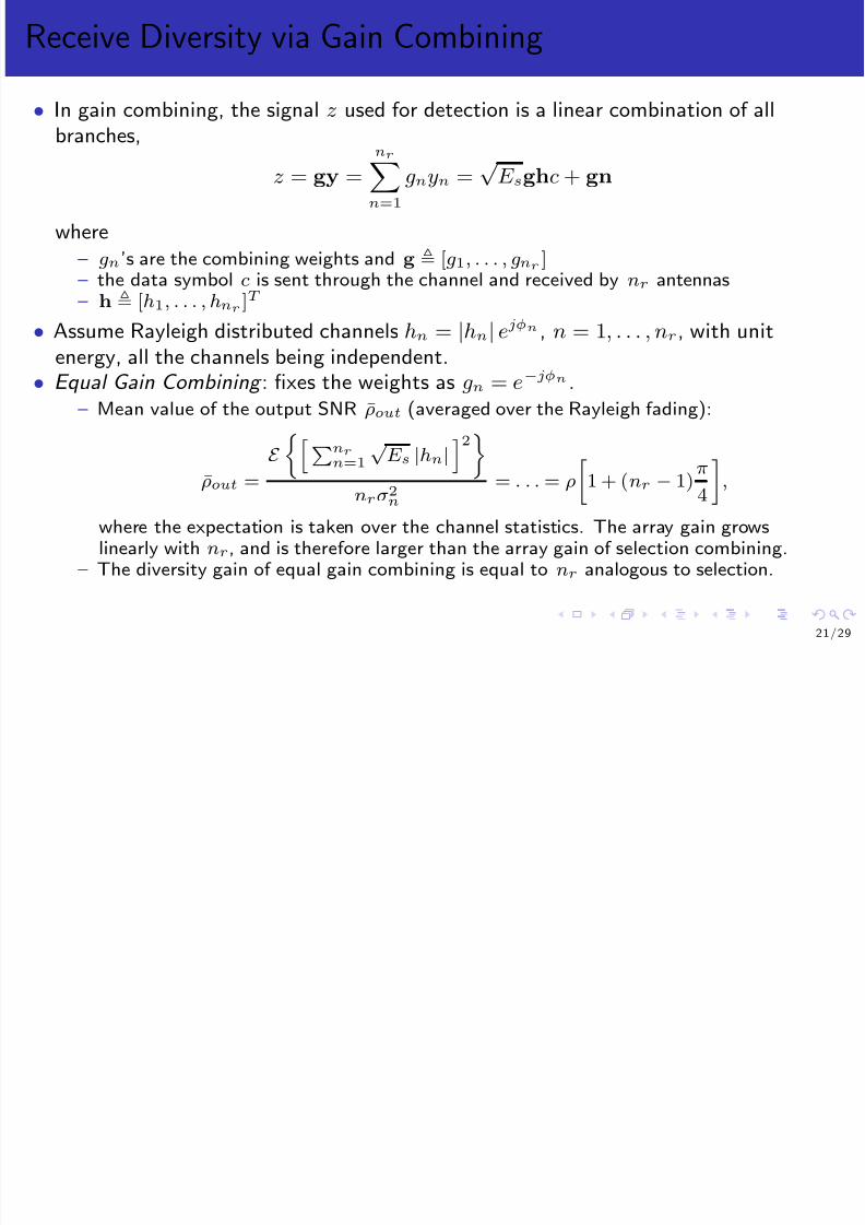
• Maximal Ratio Combining :the weights are chosen as gn = h∗n.– It maximizes the average output SNR ρout
ρout = E s
σ2nE h4h2
= ρE
h2
= ρnr.
The array gain ga is thus always equal to nr , or equivalently, the output SNR is thesum of the SNR levels of all branches (holds true irrespective of the correlationbetween the branches).
– For BPSK transmission, the symbol error rate reads as
P =
∞0
Q 2ρu
pu(u) du
where u = h2 is χ2 distribution with 2nr degrees of freedom when the differentchannels are i.i.d. Rayleigh
pu(u) =
1
(nr − 1)! u
nr−1
e
−u
.
At high SNR, P becomes
P = (4ρ)−nr
2nr − 1nr
.
The diversity gain is again equal to nr .
22/29
Receive Diversity via Gain Combining

8/12/2019 Wireless Communications Lectures
http://slidepdf.com/reader/full/wireless-communications-lectures 28/271
Receive Diversity via Gain Combining
– For alternative constellations, the error probability is given, assuming ML detection, by
P ≈ ∞0 N eQdmin ρu
2 pu(u) du,
≤ N eE
e−d2minρu
4
(using Chernoff bound Q (x) ≤ exp
−x2
2
)
where N e and dmin are respectively the number of nearest neighbors and minimumdistance of separation of the underlying constellation.
Since u is a χ2 variable with 2nr degrees of freedom, the above average upper-boundis given by
P ≤ N e
1
1 + ρd2min/4
nrρր
≤ N eρd2min4
−nr .
The diversity gain god is equal to the number of receive branches in i.i.d. Rayleighchannels.
23/29
Receive Diversity via Gain Combining

8/12/2019 Wireless Communications Lectures
http://slidepdf.com/reader/full/wireless-communications-lectures 29/271
Receive Diversity via Gain Combining
• Minimum Mean Square Error Combining – So far noise was white Gaussian. When the noise (and interference) is colored, MRC is
not optimal anymore.– Let us denote the combined noise plus interference signal as ni such thaty =
√ E shc + ni.
– An optimal gain combining technique is the minimum mean square error (MMSE)combining, where the weights are chosen in order to minimize the mean square errorbetween the transmitted symbol c and the combiner output z, i.e.,
g⋆ = arg ming
E |gy− c
|2 .
– The optimal weight vector g⋆ is given by
g⋆ = hH R−1ni ,
where Rni = E ninH i is the correlation matrix of the combined noise plusinterference signal ni.
– Such combiner can be thought of as first whitening the noise plus interference by
multiplying y by R−1/2ni and then match filter the effective channel R−1/2ni h using
hH R−H/2ni
.– The Signal to Interference plus Noise Ratio (SINR) at the output of the MMSE
combiner simply writes asρout = E sh
H R−1ni h.
– In the absence of interference and the presence of white noise, MMSE combiner
reduces to MRC filter up to a scaling factor.24/29
MISO Systems

8/12/2019 Wireless Communications Lectures
http://slidepdf.com/reader/full/wireless-communications-lectures 30/271
MISO Systems
• MISO systems exploit diversity at the transmitter through the use of nt transmitantennas in combination with pre-processing or precoding.
• A significant difference with receive diversity is that the transmitter might not havethe knowledge of the MISO channel.
– At the receiver, the channel is easily estimated.– At the transmit side, feedback from the receiver is required to inform the transmitter.
• There are basically two different ways of achieving direct transmit diversity :– when Tx has a perfect channel knowledge , beamforming can be performed to achieve
both diversity and array gains,– when Tx has a partial or no channel knowledge of the channel , space-time coding is
used to achieve a diversity gain (but no array gain in the absence of any channelknowledge).
• Indirect transmit diversity techniques convert spatial diversity to time or frequencydiversity.
25/29
Transmit Diversity via Matched Beamforming

8/12/2019 Wireless Communications Lectures
http://slidepdf.com/reader/full/wireless-communications-lectures 31/271
Transmit Diversity via Matched Beamforming
• The actual transmitted signal is a vector c′ that results from the multiplication of the signal c by a weight vector w.
• At the receiver, the signal reads as
y =√
E shc′ + n =
√ E shwc + n,
where h [h1, . . . , hnt ] represents the MISO channel vector, and w is also known asthe precoder.
• The choice that maximizes the receive SNR is given by
w = hH
h .
• Transmit along the direction of the matched channel, hence it is also known asmatched beamforming or transmit MRC .
• The array gain is equal to the number of transmit antennas, i.e. ρout = ntρ.
• The diversity gain equal to nt as the symbol error rate is upper-bounded at highSNR by
P ≤ N e
ρd2min
4
−nt.
• Matched beamforming presents the same performance as receive MRC, but requires
a perfect transmit channel knowledge .26/29
Transmit Diversity via Space-Time Coding
8/12/2019 Wireless Communications Lectures
http://slidepdf.com/reader/full/wireless-communications-lectures 32/271
y p g
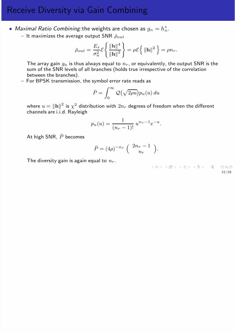
• Alamouti scheme is an ingenious transmit diversity scheme for two transmitantennas which does not require transmit channel knowledge.
– Assume that the flat fading channel remains constant over the two successive symbolperiods, and is denoted by h = [h1 h2].– Two symbols c1 and c2 are transmitted simultaneously from antennas 1 and 2 during
the first symbol period, followed by symbols −c∗2 and c∗1, transmitted from antennas 1and 2 during the next symbol period:
y1 =
E sh1
c1√ 2
+
E sh2
c2√ 2
+ n1, (first symbol period)
y2 = − E sh1 c∗2√
2+
E sh2 c∗1√ 2
+ n2. (second symbol period)
The two symbols are spread over two antennas and over two symbol periods.– Equivalently
y = y1y∗2 = E s
h1 h2h∗2
−h∗1
Heff
c1/
√ 2
c2/√
2 c
+ n1
n∗2 .
– Applying the matched filter HH eff to the received vector y effectively decouples the
transmitted symbols as shown below
z1
z2 = HH eff y1
y∗2 = E s |h1|2 + |h2|2 I2
c1/√
2c2/
√ 2 +HH eff
n1n∗2
27/29

8/12/2019 Wireless Communications Lectures
http://slidepdf.com/reader/full/wireless-communications-lectures 33/271
Indirect Transmit Diversity

8/12/2019 Wireless Communications Lectures
http://slidepdf.com/reader/full/wireless-communications-lectures 34/271
y
• It is also possible to convert spatial diversity to time or frequency diversity, which arethen exploited using well-known SISO techniques.
• Assume that nt = 2 and that the signal on the second transmit branch is– either delayed by one symbol period: the spatial diversity is converted into frequency
diversity (delay diversity)– either phase-rotated: the spatial diversity is converted into time diversity– The effective SISO channel resulting from the addition of the two branches seen by the
receiver now fades over frequency or time. This selective fading can be exploited by
conventional diversity techniques, e.g. FEC/interleaving.
29/29

8/12/2019 Wireless Communications Lectures
http://slidepdf.com/reader/full/wireless-communications-lectures 35/271
Lecture 3 and 4: MIMO Systems - Transmissionand Channel Modelling
Bruno Clerckx
EE4-65/EE9-SO27 Wireless CommunicationsDepartment of Electrical and Electronic Engineeing
Imperial College London
January 2014
1 / 2 7
Contents

8/12/2019 Wireless Communications Lectures
http://slidepdf.com/reader/full/wireless-communications-lectures 36/271
1 Introduction - Previous Lectures
2 MIMO SystemsSpace-Time CodingDominant Eigenmode TransmissionMultiple Eigenmode TransmissionMultiplexing gain
3 Double-Directional Channel Modeling
Wide-Sense Stationary Uncorrelated Scattering HomogeneousSpectraAngular Spread
4 The MIMO Channel MatrixSteering VectorsA Finite Scatterer MIMO Channel Representation
5 Statistical Properties of the MIMO Channel MatrixSpatial Correlation
6 Analytical Representation of MIMO ChannelsRayleigh MIMO ChannelsRicean MIMO Channels
2 / 2 7
Reference Book

8/12/2019 Wireless Communications Lectures
http://slidepdf.com/reader/full/wireless-communications-lectures 37/271
• Bruno Clerckx and Claude Oestges, “MIMO Wireless Networks: Channels,Techniques and Standards for Multi-Antenna, Multi-User and Multi-Cell Systems,”
Academic Press (Elsevier), Oxford, UK, Jan 2013.
– Chapter 1
Section: 1.2.4, 1.3.2, 1.6
– Chapter 2
Section: 2.1.1, 2.1.2, 2.1.3, 2.1.5, 2.2,2.3.1
– Chapter 3
Section: 3.2.1, 3.2.2, 3.4.1
3 / 2 7
Introduction - Previous Lectures (1&2)

8/12/2019 Wireless Communications Lectures
http://slidepdf.com/reader/full/wireless-communications-lectures 38/271
• Discrete Time Representation– SISO: y =
√ E shc + n
– SIMO: y =√
E shc + n
– MISO (with perfect CSIT): y = √ E shwc + n
• h is fading– amplitude Rayleigh distributed– phase uniformly distributed
• Diversity
– Diversity gain: god(ρ)
−log2(P )log2(ρ)
– Array gain: ga ρout
ρ = ρout
ρ
• SIMO– selection combining– gain combining
• MISO
– with perfect channel knowledge at Tx: Matched Beamforming– without channel knowledge at Tx: Space-Time Coding (Alamouti Scheme), indirect
(time, frequency) transmit diversity
4 / 2 7
MIMO Systems

8/12/2019 Wireless Communications Lectures
http://slidepdf.com/reader/full/wireless-communications-lectures 39/271
• In MIMO systems, the fading channel between each transmit-receive antenna paircan be modeled as a SISO channel.
• For uni-polarized antennas and small inter-element spacings (of the order of thewavelength), path loss and shadowing of all SISO channels are identical.
• Stacking all inputs and outputs in vectors ck = [c1,k , . . . , cnt,k]T andyk = [y1,k , . . . , ynr,k]T , the input-output relationship at any given time instant kreads as
yk =√
E sHkc′
k + nk,
where– c′k is a precoded version of ck that depends on the channel knowledge at the Tx.– Hk is defined as the nr × nt MIMO channel matrix, Hk(n, m) = hnm,k, with hnm
denoting the narrowband channel between transmit antenna m (m = 1, . . . , nt) andreceive antenna n (n = 1, . . . , nr),
– nk = [n1,k, . . . , nnr ,k]T is the sampled noise vector, containing the noise contribution
at each receive antenna, such that the noise is white in both time and spatialdimensions, E nknH l
= σ2
nInr δ (k − l).
• Using the same channels normalization as for SISO channels, E H2F = ntnr.• when Tx has a perfect channel knowledge : (dominant and multiple) eigenmode
transmission• when Tx has no knowledge of the channel : space-time coding (with c′k = ck)
5 / 2 7
Space-Time Coding

8/12/2019 Wireless Communications Lectures
http://slidepdf.com/reader/full/wireless-communications-lectures 40/271
• MIMO without Transmit Channel Knowledge
• Array/diversity/coding gains are exploitable in SIMO, MISO and ... MIMO
• Alamouti scheme can easily be applied to 2 × 2 MIMO channels
H =
h11 h12
h21 h22
• Received signal vector (make sure the channel remains constant over two symbol
periods!)
y1 =√
E sH c1/√ 2
c2/√
2
+ n1, (first symbol period)
y2 =√
E sH
−c∗2/√
2
c∗1/√
2
+ n2. (second symbol period)
• Equivalently
y =
y1y∗2
=
√ E s
h11 h12
h21 h22
h∗12 −h∗11h∗22 −h∗21
Heff
c1/
√ 2
c2/√
2
c
+
n1
n∗2
.
6 / 2 7
Space-Time Coding

8/12/2019 Wireless Communications Lectures
http://slidepdf.com/reader/full/wireless-communications-lectures 41/271
• Apply the matched filter HH eff to y (HH
eff Heff = H2F I2)
z = z 1z 2 = √ E sHH eff y = H2F I2 c + n′
where n′ is such that En′ = 02×1 and En′n′H = H2F σ2nI2.
• Average output SNR
ρout = E sσ2nE H2F 2
2 H2F = 2ρ,
Receive array gain (ga = nr = 2) but no transmit array gain!
• Average symbol error rate
P ≤ N eρd2min
8 −4
.
Full diversity (god = ntnr = 4)
7 / 2 7
Dominant Eigenmode Transmission

8/12/2019 Wireless Communications Lectures
http://slidepdf.com/reader/full/wireless-communications-lectures 42/271
• MIMO with Perfect Transmit Channel Knowledge• Extension of Matched Beamforming to MIMO
y = √ E sHc′ + n = √ E sHwc + n,
z = gy =√
E sgHwc + gn.
• Decompose
H = UHΣHVH
H,ΣH = diagσ1, σ2, . . . , σr(H).
• Received SNR is maximized by matched filtering, leading to
w = vmax
g = uH max
where vmax and umax are respectively the right and left singular vectorscorresponding to the maximum singular value of H, σmax = maxσ1, σ2, . . . , σr(H).Note the generalization of matched beamforming (MISO) and MRC (SIMO)!
• Equivalent channel: z =
√ E sσmaxc + n where n = gn has a variance equal to σ2
n.
8 / 2 7
Dominant Eigenmode Transmission

8/12/2019 Wireless Communications Lectures
http://slidepdf.com/reader/full/wireless-communications-lectures 43/271
• Array gain: Eσ2max = Eλmax where λmax is the largest eigenvalue of HHH .
Commonly, maxnt, nr ≤ ga ≤ ntnr.
Example
Array gain changes depending on the channel properties and distribution
– Line of Sight: H = 1nr×nt . Only one singular value is non-zero and equal to√ ntnr: ga = ntnr.
– In the i.i.d. Rayleigh case: for large nt, nr, ga = √ nt +√
nr2.
• Diversity gain: the dominant eigenmode transmission extracts a full diversity gain of ntnr in i.i.d. Rayleigh channels.
9 / 2 7
Multiple Eigenmode Transmission

8/12/2019 Wireless Communications Lectures
http://slidepdf.com/reader/full/wireless-communications-lectures 44/271
• Assume nr ≥ nt an that r (H) = nt, i.e. nt singular values in H. Hence, what aboutspreading symbols over all non-zero eigenmodes of the channel:
– Tx side: multiply the input vector c (nt
×1) using VH, i.e. c′ = VHc.
– Rx side: multiply the received vector y by G = UH H.
– Overall,
z =
E sGHc′ +Gn
=
E sUH HHVHc + UH n
= E sΣHc + n.
The channel has been decomposed into nt parallel SISO channels given byσ1, . . . , σnt.
• The rate achievable in the MIMO channel is the sum of the SISO channel capacities
R =
nt
k=1
log2(1 + ρskσ2k),
where s1, . . . , snt is the power allocation on each of the channel eigenmodes.• The capacity scales linearly in nt. By contrast, this transmission does not necessarily
achieve the full diversity gain of ntnr but does at least provide nr-fold array anddiversity gains (still assuming nt ≤ nr).
• In general, the rate scales linearly with the rank of H.
10/27
Multiplexing gain

8/12/2019 Wireless Communications Lectures
http://slidepdf.com/reader/full/wireless-communications-lectures 45/271
• Array/diversity/coding gains are exploitable in SIMO, MISO and MIMO but MIMOcan offer much more than MISO and SIMO.
• MIMO channels offer multiplexing gain: measure of the number of independentstreams that can be transmitted in parallel in the MIMO channel. Defined as
gs limρ→∞
R
ρ
log2 ρwhere R(ρ) is the transmission rate.
• The multiplexing gain is the pre-log factor of the rate at high SNR, i.e.
R
≈gs log2 ρ
• Modeling only the individual SISO channels from one Tx antenna to one Rx antennanot enough:
– MIMO performance depends on the channel matrix properties– characterize all statistical correlations between all matrix elements necessary!
11/27
Double-Directional Channel Modeling
8/12/2019 Wireless Communications Lectures
http://slidepdf.com/reader/full/wireless-communications-lectures 46/271
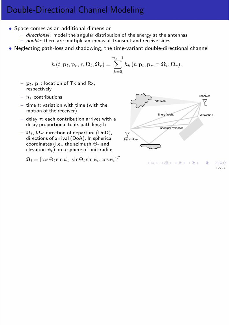
• Space comes as an additional dimension– directional : model the angular distribution of the energy at the antennas– double : there are multiple antennas at transmit and receive sides
• Neglecting path-loss and shadowing, the time-variant double-directional channel
h (t,pt,pr, τ,Ωt,Ωr) =
ns−1k=0
hk (t,pt,pr, τ,Ωt,Ωr) ,
– pt, pr : location of Tx and Rx,respectively
– ns contributions
– time t: variation with time (with themotion of the receiver)
– delay τ : each contribution arrives with a
delay proportional to its path length– Ωt, Ωr: direction of departure (DoD),
directions of arrival (DoA). In sphericalcoordinates (i.e., the azimuth Θt andelevation ψt) on a sphere of unit radius
Ωt = [cos Θt sin ψt, sinΘt sin ψt, cos ψt]T
transmitter
line-of-sight
diffusion
receiver
diffraction
specular reflection
12/27
Double-Directional Channel Modeling

8/12/2019 Wireless Communications Lectures
http://slidepdf.com/reader/full/wireless-communications-lectures 47/271
• In the case of a plane wave, and considering a fixed transmitter and a mobile receiver,
hk (t,pt,pr, τ,Ωt,Ωr) αk ejφk e−j∆ωkt δ (τ
−τ k) δ (Ωt
−Ωt,k) δ (Ωr
−Ωr,k),
where– αk is the amplitude of the kth contribution,– φk is the phase of the kth contribution,– ∆ωk is the Doppler shift of the kth contribution,– τ k is the time delay of the kth contribution,– Ωt,k is the DoD of the kth contribution,
– Ωr,k is the DoA of the kth
contribution.• A more compact notation (all temporal variations are grouped into t)
h (t,τ,Ωt,Ωr) =
ns−1k=0
hk (t,τ,Ωt,Ωr)
• Impulse response of the channel (as in Lecture 1, without path loss/shadowing)
h(t, τ ) =
h
t,τ,Ωt,Ωr
dΩt dΩr
• Narrowband transmission (the channel is not frequency selective)
h(t) = ht,τ,Ωt,Ωr dτ dΩt dΩr
13/27
Wide-Sense Stationary Uncorrelated ScatteringHomogeneous

8/12/2019 Wireless Communications Lectures
http://slidepdf.com/reader/full/wireless-communications-lectures 48/271
• Assumption: Wide-Sense Stationary Uncorrelated Scattering Homogeneous(WSSUSH) channels
• Wide-Sense Stationary:– Time correlations only depend on the time difference– Signals arriving with different Doppler frequencies are uncorrelated
• Uncorrelated Scattering:
– Frequency correlations only depend on the frequency difference– Signals arriving with different delays are uncorrelated
• Homogeneous:– Spatial correlation only depends on the spatial difference at both transmit and receive
sides
– Signals departing/arriving with different directions are uncorrelated
14/27
Spectra

8/12/2019 Wireless Communications Lectures
http://slidepdf.com/reader/full/wireless-communications-lectures 49/271
• Doppler spectrum and coherence time (see Advanced Communication Theory)• Power delay spectrum and delay spread (see Advanced Communication Theory)
• Power direction spectrum and angle spread– the power-delay joint direction spectrum
P h
τ,Ωt,Ωr
= E ht,τ,Ωt,Ωr2 ,
– the joint direction power spectrum
A(Ωt,Ωr) = P h
τ, Ωt,Ωr dτ,
– the transmit direction power spectrum
At(Ωt) =
P h
τ, Ωt,Ωr
dτ dΩr ,
– the receive direction power spectrum
Ar(Ωr) = P hτ, Ωt,Ωr
dτ dΩt.
15/27
Angular Spread

8/12/2019 Wireless Communications Lectures
http://slidepdf.com/reader/full/wireless-communications-lectures 50/271
• The channel angle-spreads are defined similarly to the delay-spread– delay-spread ⇐⇒ channel frequency selectivity– angle-spread
⇐⇒ channel spatial selectivity
Ωt,M =
ΩtAt(Ωt) dΩt At(Ωt) dΩt
Ωt,RMS =
Ωt −Ωt,M 2At(Ωt) dΩt
At(Ωt) dΩt
L=2
L=0
L=1
16/27
The MIMO Channel Matrix

8/12/2019 Wireless Communications Lectures
http://slidepdf.com/reader/full/wireless-communications-lectures 51/271
• Convert the double-directional channel to a nr × nt MIMO channel
H(t, τ ) =
h11(t, τ ) h12(t, τ ) . . . h1nt(t, τ )
h21(t, τ ) h22(t, τ ) . . . h2nt(t, τ )...
.... . .
...hnr1(t, τ ) hnr2(t, τ ) . . . hnrnt(t, τ )
,
where
hnm(t, τ )
hnm
t,τ,Ωt,Ωr
dΩt dΩr
• For narrowband (i.e. same delay for all antennas) balanced (i.e. |hnm| = |h11|) arraysand plane wave incidence, hnm
t,τ,Ωt,Ωr
is a phase shifted version of
h11t,τ,Ωt,Ωrhnm(t, τ ) =
h11
t,τ,Ωt,Ωr
e−jkT r (Ωr)
p(n)r −p
(1)r
e−jkT t (Ωt)
p(m)t −p
(1)t
dΩtdΩr
where kt(Ωt) and kr(Ωr) are the transmit and receive wave propagation 3 × 1vectors.
17/27
Steering Vectors

8/12/2019 Wireless Communications Lectures
http://slidepdf.com/reader/full/wireless-communications-lectures 52/271
• For a transmit ULA oriented broadside to the link axis,
e
−jkT t (Ωt)·p(m)t −p
(1)t = e
−j(m−1)ϕt(θt)
,where ϕt (θt) = 2π(dt/λ)cos θt, and dt =
p(m)t − p
(m−1)t
denotes theinter-element spacing of the transmit array.
– θt is defined relatively to the array orientation (so θt = π/2 corresponds to the link axisfor a broadside array).
• Steering vector (expressed here for a ULA)– At the transmitter in the relative direction θt:
at(θt) = [ 1 e−jϕt(θt) . . . e−j(nt−1)ϕt(θt) ]T .
– At the receiver in the relative direction θr:
ar (θr) = [ 1 e−jϕr(θr) . . . e−j(nr−1)ϕr(θr) ]T .
• Under the plane wave and balanced narrowband array assumptions, the MIMOchannel matrix can be rewritten as a function of steering vectors as
H(t, τ ) =
h
t,p
(1)t ,p(1)r , τ,Ωt,Ωr
ar(Ωr) aT t (Ωt) dΩt dΩr.
18/27

8/12/2019 Wireless Communications Lectures
http://slidepdf.com/reader/full/wireless-communications-lectures 53/271
Statistical Properties of the MIMO Channel Matrix

8/12/2019 Wireless Communications Lectures
http://slidepdf.com/reader/full/wireless-communications-lectures 54/271
• Assume narrowband channels, the spatial correlation matrix of the MIMO channel
R =
Evec(HH )vec(HH )H
This is a ntnr × ntnr positive semi-definite Hermitian matrix.
• It describes the correlation between all pairs of transmit-receive channels:– E H(n, m)H∗(n, m): the average energy of the channel between antenna m and
antenna n,
– r(nq)m = E H(n, m)H∗(q, m): the receive correlation between channels originating
from transmit antenna m and impinging upon receive antennas n and q,
– t(mp)n = E H(n, m)H∗(n, p): the transmit correlation between channels originating
from transmit antennas m and p and arriving at receive antenna n,– E H(n, m)H∗(q, p): the cross-channel correlation between channels (m, n) and
(q, p).
Example
2x2 MIMO
R =
1 t∗1 r∗1 s∗1t1 1 s∗2 r∗2r1 s2 1 t∗2s1 r2 t2 1
t1 = E H(1, 1)H∗(1, 2)r1 = E H(1, 1)H∗(2, 1)
20/27

8/12/2019 Wireless Communications Lectures
http://slidepdf.com/reader/full/wireless-communications-lectures 55/271
Spatial Correlation

8/12/2019 Wireless Communications Lectures
http://slidepdf.com/reader/full/wireless-communications-lectures 56/271
• When the energy spreading is very large at both sides and dt/dr are sufficientlylarge, elements of H become uncorrelated, and R becomes diagonal.
Example
Consider two transmit antennas spaced by dt. The transmit correlation writesas
t =
2π0
ej2π(dt/λ) cos θtAt(θt)dθt,
which only depends on the transmit antenna spacing and the transmit directionpower spectrum.
– isotropic scattering : very rich scattering environment around the transmitter witha uniform distribution of the energy, i.e. At(θt) ∼= 1/2π
t = 1
2π 2π
0ejϕt(θt)dθt =
1
2π 2π
0ej2π(dt/λ) cos θtdθt
= J0
2π
dt
λ
.
The transmit correlation only depends on the spacing between the two antennas.
22/27
Spatial Correlation
8/12/2019 Wireless Communications Lectures
http://slidepdf.com/reader/full/wireless-communications-lectures 57/271
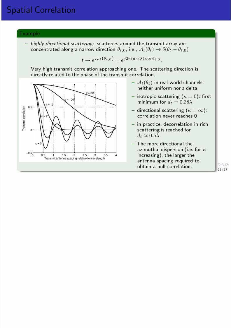
Example
– highly directional scattering : scatterers around the transmit array areconcentrated along a narrow direction θt,0, i.e., At(θt) → δ(θt − θt,0)
t → ejϕt(θt,0) = ej2π(dt/λ) cos θt,0 .
Very high transmit correlation approaching one. The scattering direction isdirectly related to the phase of the transmit correlation.
0 0.5 1 1.5 2 2.5 3 3.5 4−0.5
0
0.5
1
Transmit antenna spacing relative to wavelength
T r a n s m i t c o r r e l a t i o n
κ = 0
κ = 10
κ = 100
κ = 500
κ = 2
– A
t(θt) in real-world channels:neither uniform nor a delta.
– isotropic scattering (κ = 0): firstminimum for dt = 0.38λ
– directional scattering (κ = ∞):correlation never reaches 0
– in practice, decorrelation in richscattering is reached fordt ≈ 0.5λ
– The more directional theazimuthal dispersion (i.e. for κincreasing), the larger theantenna spacing required to
obtain a null correlation. 23/27
Analytical Representation of Rayleigh MIMO Channels

8/12/2019 Wireless Communications Lectures
http://slidepdf.com/reader/full/wireless-communications-lectures 58/271
• Independent and Identically Distributed (I.I.D.) Rayleigh fading– R = Intnr– H = Hw is a random fading matrix with unit variance and i.i.d. circularly symmetric
complex Gaussian entries.• Realistic in practice only if both conditions are satisfied:– the antenna spacings and/or the angle spreads at Tx and Rx are large enough,– all individual channels characterized by the same average power (i.e., balanced array).
• What about real-world channels? Sometimes significantly deviate from this idealchannel:
– limited angular spread and/or reduced array sizes cause the channels to becomecorrelated (channels are not independentanymore)
– a coherent contribution may induce thechannel statistics to become Ricean
(channels are not Rayleigh distributedanymore),
– the use of multiple polarizations createsgain imbalances between the variouselements of the channel matrix (channelsare not identically distributed anymore).
24/27
Correlated Rayleigh Fading Channels

8/12/2019 Wireless Communications Lectures
http://slidepdf.com/reader/full/wireless-communications-lectures 59/271
• For identically distributed Gaussian channels, R constitutes a sufficient description of the stochastic behavior of the MIMO channel.
• Any channel realization is obtained byvec
H
H = R1/2 vec(Hw),
where Hw is one realization of an i.i.d. channel matrix.• Complicated to use because
– cross-channel correlation not intuitive and not easily tractable– Too many parameters: dimensions of R rapidly become large as the array sizes increase
– vec operation complicated for performance analysis• Kronecker model: use a separability assumption
R = Rr ⊗Rt,
H = R1/2r HwR
1/2t
where Rt and Rr are respectively the transmit and receive correlation matrices.
• Striclty valid only if r1 = r2 = r and t1 = t2 = t and s1 = rt and s2 = rt∗ (for 2× 2)
R =
1 t∗1 r∗1 s∗1t1 1 s∗2 r∗2r1 s2 1 t∗2s1 r2 t2 1
=
1 t∗ r∗ r∗t∗
t 1 r∗t r∗
r rt∗ 1 t∗
rt r t 1
=
1 r∗
r 1
Rr
⊗
1 t∗
t 1
Rt
25/27
Analytical Representation of Ricean MIMO Channels

8/12/2019 Wireless Communications Lectures
http://slidepdf.com/reader/full/wireless-communications-lectures 60/271
• In the presence of a strong coherent component which does not experience anyfading over time
– e.g. a line-of-sight field, one or several specular contributions, coherent addition of
reflected and diffracted contributions (in fixed wireless access only).• All these situations lead to a Ricean distribution of the received field amplitude.
– The relative strength of the dominant coherent component is characterized by theK-factor K . As the channel contains a coherent component, its amplitude can bewritten as
|h(t)| = h + h(t) ,
where h is the coherent component, and h(t) is the non coherent part, whose energy isdenoted as 2σ2
s .– The K-factor is defined as
K =
h22σ2
s
.
–
|h(t)
| s′ is Ricean distributed, and its distribution is given, as a function of K , as
ps′ (s′) = 2s′K h2 exp
−K
s′2h2 + 1
I0
2s′K h
.
– For K = 0, the Ricean distribution boils down to the Rayleigh distribution while forK = ∞, the channel becomes deterministic (no fading).
26/27
Ricean MIMO Channels

8/12/2019 Wireless Communications Lectures
http://slidepdf.com/reader/full/wireless-communications-lectures 61/271
• Common Ricean MIMO channel model
H = K
1 + K ¯H + 1
1 + K ˜H
• The matrix H relates to the Rayleigh component (non-coherent part). It can bemodeled and characterized using
R = Evec(HH )vec(HH )H • The matrix H corresponding to the coherent component(s) has fixed phase-shift-only
entries (strongly related to the array configuration and orientation)
H =
ejα11 ejα12
ejα21 ejα22
– With only one coherent contribution with given DoD and DoA (Ωt,c and Ωr,c),
H = ar(Ωr,c) aT t (Ωt,c)
– For broadside arrays with a pure line-of-sight component, H = 1nr×nt .
27/27

8/12/2019 Wireless Communications Lectures
http://slidepdf.com/reader/full/wireless-communications-lectures 62/271
Lecture 5 and 6: Capacity of point-to-point
MIMO Channels
Bruno Clerckx
EE4-65/EE9-SO27 Wireless CommunicationsDepartment of Electrical and Electronic Engineeing
Imperial College London
January 2014
1 / 2 3
Contents

8/12/2019 Wireless Communications Lectures
http://slidepdf.com/reader/full/wireless-communications-lectures 63/271
1 Introduction - Previous Lectures
2 System Model
3 Capacity of Deterministic MIMO Channels
4 Ergodic Capacity of Fast Fading ChannelsI.I.D. Rayleigh Fast Fading ChannelsCorrelated Rayleigh Fast Fading Channels
5 Outage Capacity and Probability in Slow Fading Channels
6 Diversity-Multiplexing Trade-Off
2 / 2 3
Reference Book

8/12/2019 Wireless Communications Lectures
http://slidepdf.com/reader/full/wireless-communications-lectures 64/271
• Bruno Clerckx and Claude Oestges, “MIMO Wireless Networks: Channels,Techniques and Standards for Multi-Antenna, Multi-User and Multi-Cell Systems,”Academic Press (Elsevier), Oxford, UK, Jan 2013.
– Chapter 5
Section: 5.1, 5.2, 5.3, 5.4.1, 5.4.2(except “Antenna Selection Schemes”),5.5.1 - “Kronecker Correlated RayleighChannels”, 5.5.2, 5.7, 5.8.1 (exceptProof of Proposition 5.9 and Example5.4)
3 / 2 3
Introduction - Previous Lectures (3&4)
• Transmission strategies

8/12/2019 Wireless Communications Lectures
http://slidepdf.com/reader/full/wireless-communications-lectures 65/271
• Transmission strategies– Space-Time Coding when no Tx channel knowledge– Multiple (including dominant) eigenmode transmission when Tx channel knowledge
z =
E sGHc′ +Gn
=
E sUH HHVHc+ UH n
=
E sΣHc + n.
Multiple parallel data pipes → Spatial multiplexing gain!
• Performance highly depends on the channel matrix properties– Angle spread and inter-element spacing– Spatial Correlation: spread antennas far apart to decrease spatial correlation– Rayleigh and Ricean distribution
4 / 2 3
System Model
A i l MIMO i h i d i

8/12/2019 Wireless Communications Lectures
http://slidepdf.com/reader/full/wireless-communications-lectures 66/271
• A single-user MIMO system with nt transmit and nr receive antennas over afrequency flat-fading channel.
• The transmit and received signals in a MIMO channel are related by
yk =√
E sHkc′k + nk
where– yk is the nr × 1 received signal vector,– Hk is the nr × nt channel matrix
– n
k is a nr × 1 zero mean complex additive white Gaussian noise (AWGN) vector withEnknH l = σ2
nInr δ (k − l).
– ρ = E s/σ2n represents the SNR.
• The input covariance matrix is defined as the covariance matrix of the transmitsignal c′ (we drop the time index) and writes as Q = E c′c′H
.• Short-term power constraint: TrQ ≤ 1.
• Long-term power constraint (over a duration duration T p >> T ): E TrQ ≤ 1where the expectation refers here to the averaging over successive codeword of length T .
• Channel time variation: T coh coherence time– slow fading : T coh is so long that coding is performed over a single channel realization.– fast fading : T coh is so short that coding over multiple channel realizations is possible.
5 / 2 3
Capacity of Deterministic MIMO Channels

8/12/2019 Wireless Communications Lectures
http://slidepdf.com/reader/full/wireless-communications-lectures 67/271
Proposition
For a deterministic MIMO channel H, the mutual information I is written as
I (H,Q) = log2 det
Inr + ρHQHH
where Q is the input covariance matrix whose trace is normalized to unity.
Definition
The capacity of a deterministic nr × nt MIMO channel with perfect channelstate information at the transmitter is
C (H) = maxQ≥0:TrQ=1
log2 det Inr + ρHQHH .
Note the difference with SISO capacity.
6 / 2 3
Capacity and Water-Filling Algorithm
Wh t i th b t t i i t t i th ti i t i t i Q?

8/12/2019 Wireless Communications Lectures
http://slidepdf.com/reader/full/wireless-communications-lectures 68/271
• What is the best transmission strategy, i.e. the optimum input covariance matrix Q?• First , create n = minnt, nr parallel data pipes (Multiple Eigenmode Transmission)
– Decouple the channel along the individual channel modes (in the directions of the
singular vectors of the channel matrix H at both the transmitter and the receiver)
H = UHΣHVH H,
UH HHVH = UH
HUHΣHVH HVH = ΣH
– Optimum input covariance matrix Q⋆ writes as
Q⋆ = VHdiag s⋆1, . . . , s⋆nVH H,
• Second , allocate power to data pipes– ΣH = diag σ1, . . . , σn, and σ2k λk
– Capacity: C (H) = maxsknk=1
nk=1 log2
1 + ρskλk
= n
k=1 log2
1 + ρs⋆kλk
Proposition
The power allocation strategy s1, . . . , sn = s
⋆
1, . . . , s
⋆
n that maximizes n
k=1 log2 (1 + ρλksk) under the power constraint n
k=1 sk = 1, is given by the water-filling solution,
s⋆k =
µ −
1
ρλk
+, k = 1, . . . , n
where µ is chosen so as to satisfy the power constraint
nk=1 s⋆k = 1.
7 / 2 3
Water-Filling Algorithm
• Iterative power allocation

8/12/2019 Wireless Communications Lectures
http://slidepdf.com/reader/full/wireless-communications-lectures 69/271
• Iterative power allocation
– Order eigenvalues λk in decreasing order
of magnitude– At iteration i, evaluate the constant µ
from the power constraint
µ(i) = 1
n − i + 1
1 +
n−i+1k=1
1
ρλk
– Calculate power
sk(i) = µ(i) − 1
ρλk,
k = 1, . . . , n− i + 1.
If sn−i+1 < 0, set to 0
– Iterate till the power allocated on eachmode is non negative.
∗
1s
∗
2s
∗
3s
. . .
1
1
ρ λ 2
1
ρ λ
3
1
ρ λ
1
1
-n ρ λ
n ρ λ
1
µ
8 / 2 3

8/12/2019 Wireless Communications Lectures
http://slidepdf.com/reader/full/wireless-communications-lectures 70/271
Ergodic Capacity of Fast Fading Channels
• Fast fading:

8/12/2019 Wireless Communications Lectures
http://slidepdf.com/reader/full/wireless-communications-lectures 71/271
• Fast fading:– Doppler frequency sufficiently high to allow for coding over many channel
realizations/coherence time periods
– The transmission capability is represented by a single quantity known as the ergodiccapacity
• MIMO Capacity with Perfect Transmit Channel Knowledge– similar strategy as in deterministic channels: transmit along eigenvectors of channel
matrix and allocate power following water-filling– short term power constraint: water-filling solution applied over space as in
deterministic channels
C CSIT,ST = E
max
Q≥0:TrQ=1log2 det
Inr + ρHQHH
=
nk=1
E
log2
1 + ρs⋆kλk
.
– long term power constraint: water-filling solution applied over both time and space
C CSIT,LT =n
k=1
E
log2
1 + ρs⋆
kλk
.
– Impact on coding strategy? Use a variable-rate code (family of codes of different rates)adapted as a function of the water-filling allocation. No need for the codeword to spanmany coherence time periods.
10/23
MIMO Capacity with Partial Transmit Channel Knowledge
• H is not known to the transmitter → we cannot adapt Q at all time instants

8/12/2019 Wireless Communications Lectures
http://slidepdf.com/reader/full/wireless-communications-lectures 72/271
• H is not known to the transmitter → we cannot adapt Q at all time instants• Rate of information flow between Tx and Rx at time instant k over channels Hk
log2 detInr + ρHkQHH k
.
Such a rate varies over time according to the channel fluctuations. The average rateof information flow over a time duration T >> T coh is
1
T
T −1
k=0
log2 det Inr + ρHkQHH k .
Definition
The ergodic capacity of a nr × nt MIMO channel with channel distributioninformation at the transmitter (CDIT) is given by
C CDIT C = maxQ≥0:TrQ=1
E log2 detInr + ρHQHH
,
where Q is the input covariance matrix optimized as to maximize the ergodicmutual information.
• T >> T c to average out the noise and the channel fluctuations
11/23
I.I.D. Rayleigh Fast Fading Channels: Perfect TransmitChannel Knowledge
• Low SNR: allocate all the available power to the strongest or dominant eigenmode.

8/12/2019 Wireless Communications Lectures
http://slidepdf.com/reader/full/wireless-communications-lectures 73/271
• Low SNR: allocate all the available power to the strongest or dominant eigenmode.Use log2(1 + x) ≈ x log2 (e) for x small and get
C CSIT,ST = E
log2
1 + ρλmax
∼= ρE λmax
log2(e)
∼= ρn log2(e), N >> n.
¯C CSIT,LT = E log2
1 + ρs
⋆
maxλmax
∼= ρE s⋆maxλmax
log2(e)
Observations: C CSIT grows linearly in the minimum number of antennas n.• High SNR: uniform power allocation on all non-zeros eigenmodes
C CSIT ∼=
nk=1
E
log2
1 +
ρ
nλk
∼= nlog2
ρ
n
+ E
nk=1
log2(λk)
.
Observations: C CSIT also scales linearly with n. The spatial multiplexing gain isgs = n. MISO fading channels do not offer any multiplexing gain.
12/23
I.I.D. Rayleigh Fast Fading Channels: Partial TransmitChannel Knowledge
• Optimal covariance matrix

8/12/2019 Wireless Communications Lectures
http://slidepdf.com/reader/full/wireless-communications-lectures 74/271
Optimal covariance matrix
Proposition
In i.i.d. Rayleigh fading channels, the ergodic capacity with CDIT is achieved under an equal power allocation scheme Q = Int/nt, i.e.,
C CDIT = ¯ I e = E
log2 det
Inr +
ρ
ntHwH
H w
= E
nk=1
log2
1 +
ρ
ntλk
.
Encoding requires a fixed-rate code (whose rate is given by the ergodic capacity)with encoding spanning many channel realizations.
• Low SNR:
C CDIT
≥ E log21 +
ρ
nt Hw
2F ≈
ρ
nt E Hw
2F log2 (e) = nrρ log2 (e)
Observations:– C CDIT is only determined by the energy of the channel.– A MIMO channel only yields a nr gain over a SISO channel. Increasing the number of
transmit antennas is not useful (contrary to perfect CSIT). SIMO and MIMO channelsreach the same capacity for a given nr .
13/23
I.I.D. Rayleigh Fast Fading Channels: Partial TransmitChannel Knowledge
• High SNR:

8/12/2019 Wireless Communications Lectures
http://slidepdf.com/reader/full/wireless-communications-lectures 75/271
g
C CDIT ≈ E nk=1
log2 ρ
nt λk
= nlog2 ρ
nt
+ E nk=1
log2(λk)
Observations:– C CDIT at high SNR scales linearly with n (by contrast to the low SNR regime).– The multiplexing gain gs is equal to n, similarly to the CSIT case.– C CDIT and C CSIT are not equal: constant gap equal to n log2(nt/n) at high SNR.
• Expressions can be particularized to SISO, SIMO, MISO cases. At high SNR,– SISO (N = n = 1):
C CDIT ≈ log2(ρ) + E
log2
|h|2
= log2(ρ) − 0.83 = C AWGN − 0.83
– SIMO (nt = n = 1, nr = N ):
¯C CDIT ≈ log2(nrρ)
– MISO (nr = n = 1, nt = N ):
C CDIT ≈ log2(ρ) + E
log2
h2 /nt
nt→∞≈ log2(ρ) = C AWGN
14/23
I.I.D. Rayleigh Fast Fading Channels
• Ergodic capacity of various nr × nt i.i.d. Rayleigh channels with full (CSIT) and

8/12/2019 Wireless Communications Lectures
http://slidepdf.com/reader/full/wireless-communications-lectures 76/271
Ergodic capacity of various nr × nt i.i.d. Rayleigh channels with full (CSIT) andpartial (CDIT) channel knowledge at the transmitter.
−10 −5 0 5 10 15 200
2
4
6
8
10
12
14
16
18
20
SNR [dB]
E r g o d i c c a p a c i t y [ b p
s / H z ]
2 x 2 (CSIT)4 x 2 (CSIT)2 x 4 (CSIT)4 x 4 (CSIT)2 x 2 (CDIT)4 x 2 (CDIT)
2 x 4 (CDIT)4 x 4 (CDIT)
15/23
Correlated Rayleigh Fast Fading Channels: Uniform PowerAllocation
• Assume the channel covariance matrix is unknown to the transmitter

8/12/2019 Wireless Communications Lectures
http://slidepdf.com/reader/full/wireless-communications-lectures 77/271
• Mutual information with identity input covariance matrix
¯ I e = E
log2detInr + ρ
ntHH
H
.
• Low SNR
¯ I e ≥ E log21 + ρ
ntH2F .
• High SNR in Kronecker Correlated Rayleigh Channels H = R1/2r HwR
1/2t (with full
rank correlation matrices) and nt = nr
¯ I e ≈ E log2det ρ
ntHwH
H w + log2det(Rr) + log2det(Rt).
Observations:– det(Rr) ≤ 1 and det(Rt) ≤ 1: receive and transmit correlations always degrade the
mutual information (with power uniform allocation) with respect to the i.i.d. case.– ¯ I e still scales linearly with minnt, nr
16/23
Correlated Rayleigh Fast Fading Channels: PartialTransmit Channel Knowledge
• Assume the channel covariance matrix is known to the transmitter.

8/12/2019 Wireless Communications Lectures
http://slidepdf.com/reader/full/wireless-communications-lectures 78/271
Proposition
In Kronecker correlated Rayleigh fast fading channels, the optimal input covariance matrix can again be expressed as
Q = URtΛQU
H Rt
,
where URt is a unitary matrix formed by the eigenvectors of Rt (arranged in
such order that they correspond to decreasing eigenvalues of Rt), and ΛQ is adiagonal matrix whose elements are also arranged in decreasing order.
Power allocation has to be computed numerically. Approximation using Jensen’sinequality is possible.
• Spatial correlation: beneficial or detrimental?
– receive correlations degrade both the mutual information ¯ I e and the capacity withCDIT,
– transmit correlations always decrease ¯ I e but may increase C CDIT at low SNR(irrespective of nt and nr) or at higher SNR when nt > nr (analogous to the full CSITcase).
17/23
Correlated Rayleigh Fast Fading Channels: PartialTransmit Channel Knowledge
• Mutual information of various strategies at 0 dB SNR as a function of the transmit

8/12/2019 Wireless Communications Lectures
http://slidepdf.com/reader/full/wireless-communications-lectures 79/271
gcorrelation |t| in TIMO. Beamforming refers here to the tranmsission of one streamalong the dominant eigenvector of Rt.
0 0.2 0.4 0.6 0.8 12.6
2.7
2.8
2.9
3
3.1
3.2
3.3
3.4
3.5
3.6
Magnitude of transmit correlation
M u t u a
l i n f o r m a t i o n / c a p a c i t y [ b p s / H z ]
Optimal allocationEqui−power allocationBeamforming
18/23
Outage Capacity and Probability in Slow Fading Channels
• In slow fading, the encoding still averages out the randomness of the noise but

8/12/2019 Wireless Communications Lectures
http://slidepdf.com/reader/full/wireless-communications-lectures 80/271
cannot fully average out the randomness of the channel.
• For a given channel realization H and a target rate R, reliable transmission if
log2 detInr + ρHQHH
> R
If not met with any Q, an outage occurs and the decoding error probability is strictlynon-zero.
• Look at the tail probability of log2 det Inr + ρHQHH
, not its average!
Definition
The outage probability P out (R) of a nr × nt MIMO channel with a target rateR is given by
P out (R) = minQ≥0:TrQ≤1
P log2 detInr + ρHQHH < R ,
where Q is the input covariance matrix optimized as to minimize the outageprobability.
• More meaningful in the absence of CSI knowledge at the transmitter: the transmittercannot adjust its transmit strategy
→ hopes the channel is good enough
19/23
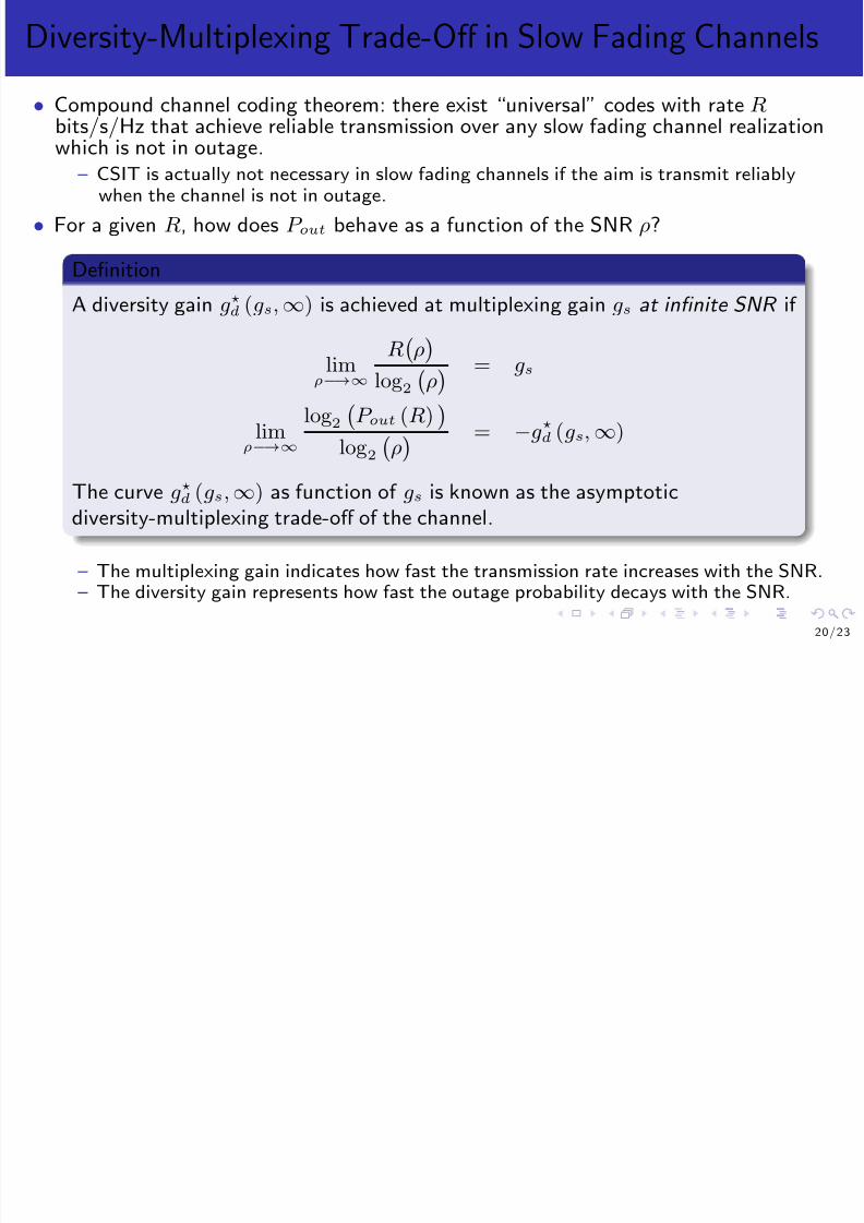
Diversity-Multiplexing Trade-Off in Slow Fading Channels
• Compound channel coding theorem: there exist “universal” codes with rate Rbits/s/Hz that achieve reliable transmission over any slow fading channel realization
8/12/2019 Wireless Communications Lectures
http://slidepdf.com/reader/full/wireless-communications-lectures 81/271
bits/s/Hz that achieve reliable transmission over any slow fading channel realizationwhich is not in outage.
– CSIT is actually not necessary in slow fading channels if the aim is transmit reliablywhen the channel is not in outage.
• For a given R, how does P out behave as a function of the SNR ρ?
Definition
A diversity gain g⋆d (gs,
∞) is achieved at multiplexing gain gs at infinite SNR if
limρ−→∞
R
ρ
log2
ρ = gs
limρ−→∞
log2
P out (R)
log2 ρ = −g⋆
d (gs,∞)
The curve g⋆d (gs,∞) as function of gs is known as the asymptotic
diversity-multiplexing trade-off of the channel.
– The multiplexing gain indicates how fast the transmission rate increases with the SNR.– The diversity gain represents how fast the outage probability decays with the SNR.
20/23
Diversity-Multiplexing Trade-Off in I.I.D. Rayleigh SlowFading Channels
• Point (0 n n ): for a spatial

8/12/2019 Wireless Communications Lectures
http://slidepdf.com/reader/full/wireless-communications-lectures 82/271
• Point (0, ntnr): for a spatialmultiplexing gain of zero (i.e., R is
fixed), the maximal diversity gainachievable is ntnr .
• Point (min nt, nr , 0):transmitting at diversity gain g⋆
d = 0(i.e., P out is kept fixed) allows thedata rate to increase with SNR asn = min nt, nr.
• Intermediate points: possible totransmit at non-zero diversity andmultiplexing gains but that anyincrease of one of those quantities
leads to a decrease of the otherquantity.
Spatial multiplexing gaing
D i v e
r s i t y g a i n g * ( g ,
)
(0,nt nr )
(1,(nt −1)(nr −1))
(2,(nt −2)(nr −2))
(g , (n − g )(n − g ))r
(min(nt ,nr ),0)
d
s
s
s sst
∞
21/23
Diversity-Multiplexing Trade-Off in I.I.D. Rayleigh SlowFading Channels

8/12/2019 Wireless Communications Lectures
http://slidepdf.com/reader/full/wireless-communications-lectures 83/271
• For fixed rates R = 2, 4, ..., 40
bits/s/Hz,– The asymptotic slope of each
curve is four and matches themaximum diversity gain g⋆
d (0,∞).
– The horizontal separation is 2
bits/s/Hz per 3 dB, whichcorresponds to the maximummultiplexing gain equal to n(= 2).
• As the rate increases more rapidlywith SNR (i.e., as the multiplexing
gain gs increases), the slope of theoutage probability curve (given bythe diversity gain g∗d) vanishes.
0 10 20 30 40 50 6010
5
104
103
102
101
100
SNR [dB]
O u t a g e
p r o b a b i l i t y P o u t
g =1.75g =0.25
g =1.5
g =0.5
g =1.25
g =0.75
g =1.0g =1.0
g =0.75g =1.75g =0.5
g =2.5
s
d *
s
s
s
s
s
*
*
*
*
*
d
d
d
d
d
Figure: 2 × 2 MIMO i.i.d. Rayleigh fading channels
22/23
Diversity-Multiplexing Trade-Off of a Scalar RayleighChannel h
• Determine for a transmission rate R scaling with ρ as gs log2 (ρ), the rate at whichthe outage probability decreases with ρ as ρ increases

8/12/2019 Wireless Communications Lectures
http://slidepdf.com/reader/full/wireless-communications-lectures 84/271
the outage probability decreases with ρ as ρ increases.
• Outage probability
P out (R) = P
log2
1 + ρ |h|2 < gs log2 (ρ)
= P
1 + ρ |h|2 < ρgs
• At high SNR,
P out (R)≈
P |h|2
≤ρ−(1−gs)
• Since |h|2 is exponentially distributed, i.e., P |h|2 ≤ ǫ
≈ ǫ for small ǫ
P out (R) ≈ ρ−(1−gs)
An outage occurs at high SNR when
|h
|2
≤ρ−(1−gs) with a probability ρ−(1−gs).
• DMT for the scalar Rayleigh fading channel g⋆d (gs,∞) = 1 − gs for gs ∈ [0, 1].
23/23

8/12/2019 Wireless Communications Lectures
http://slidepdf.com/reader/full/wireless-communications-lectures 85/271
Lecture 7,8 and 9: Space-Time Coding over I.I.D.Rayleigh Flat Fading Channels
Bruno Clerckx
EE4-65/EE9-SO27 Wireless CommunicationsDepartment of Electrical and Electronic Engineeing
Imperial College London
January 2014
1 / 5 1
Contents
1 Introduction - Previous Lectures

8/12/2019 Wireless Communications Lectures
http://slidepdf.com/reader/full/wireless-communications-lectures 86/271
2 Overview of a Space-Time Encoder
3 System Model
4 Error Probability Motivated Design MethodologyFast Fading MIMO Channels: The Distance-Product CriterionSlow Fading MIMO Channels: The Rank-Determinant Criterion
5 Information Theory Motivated Design MethodologyFast Fading MIMO Channels: Achieving The Ergodic CapacitySlow Fading MIMO Channels - Achieving The Diversity-Multiplexing Trade-Off
6 Space-Time Block CodingA General Framework for Linear STBCsSpatial Multiplexing/V-BLAST/D-BLASTOrthogonal Space-Time Block CodesOther Code ConstructionsGlobal Performance Comparison
2 / 5 1
Reference Book
• Bruno Clerckx and Claude Oestges, “MIMO Wireless Networks: Channels,Techniques and Standards for Multi-Antenna Multi-User and Multi-Cell Systems ”

8/12/2019 Wireless Communications Lectures
http://slidepdf.com/reader/full/wireless-communications-lectures 87/271
Techniques and Standards for Multi Antenna, Multi User and Multi Cell Systems,Academic Press (Elsevier), Oxford, UK, Jan 2013.
– Chapter 6
Section: 6.1, 6.2, 6.3 (except “AntennaSelection” in 6.3.2), 6.4.1, 6.4.2 (exceptthe Proofs), 6.5.1, 6.5.2, 6.5.3, 6.5.4,6.5.8, Figure 7.1
3 / 5 1
Introduction - Previous Lectures
• Lecture 5&6– Capacity of deterministic MIMO channels

8/12/2019 Wireless Communications Lectures
http://slidepdf.com/reader/full/wireless-communications-lectures 88/271
p y
C (H) = maxQ≥0:TrQ=1 log2 detInr + ρHQH
H .
– Ergodic capacity of fast fading channels– Outage capacity and probability of slow fading channels
• MIMO provides huge gains in terms of reliability and transmission rate– diversity gain, array gain, coding gain, spatial multiplexing gain
• What we further need– practical methodologies to achieve these gains?– how to code across space and time?– Some preliminary answers: multimode eigenmode transmission when channel knowledge
available at the Tx, Alamouti scheme when no channel knowledge available at the Tx
4 / 5 1
Overview of a Space-Time Encoder
• Space-time encoder: sequence of two black boxes
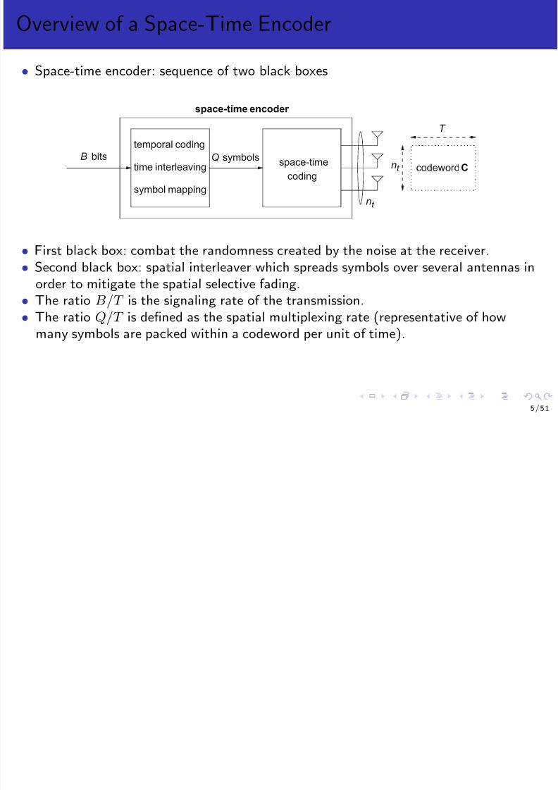
8/12/2019 Wireless Communications Lectures
http://slidepdf.com/reader/full/wireless-communications-lectures 89/271
bits
space-time encoder
nt
codewordC
T
nt
temporal coding
symbol mapping
time interleavingsymbolsQB
space-time
coding
• First black box: combat the randomness created by the noise at the receiver.• Second black box: spatial interleaver which spreads symbols over several antennas in
order to mitigate the spatial selective fading.
• The ratio B/T is the signaling rate of the transmission.
• The ratio Q/T is defined as the spatial multiplexing rate (representative of howmany symbols are packed within a codeword per unit of time).
5 / 5 1
System Model
• MIMO system with nt transmit and nr receive antennas over a frequency flat-fadingchannel

8/12/2019 Wireless Communications Lectures
http://slidepdf.com/reader/full/wireless-communications-lectures 90/271
• Transmit a codeword C = [c0 . . . cT −1] [nt
×T ] contained in the codebook
C• At the kth time instant, the transmitted and received signals are related by
yk =√
E sHkck + nk
where– yk is the nr × 1 received signal vector,– Hk is the nr
×nt channel matrix,
– nk is a nr × 1 zero mean complex AWGN vector with EnknH l = σ2nInrδ (k − l),
– The parameter E s is the energy normalization factor. SNR ρ = E s/σ2n.
• No transmit channel knowledge but we know it is i.i.d. Rayleigh fading.• Codeword average transmit power E Tr
CCH
= T . Assume
E H2F
= ntnr.
• Channel time variation:– slow fading : T coh >> T and Hk = HwT −1k=0 , with Hw denoting an i.i.d. random
fading matrix with unit variance circularly symmetric complex Gaussian entries.
– fast fading : T ≥ T coh and Hk = Hk,w , whereHk,w
T −1k=0
are uncorrelated matrices,
eachHk,w
being an i.i.d. random fading matrix with unit variance circularly
symmetric complex Gaussian entries.
6 / 5 1
Error Probability Motivated Design Methodology
• With instantaneous channel realizations perfectly known at the receive side, the MLdecoder computes an estimate of the transmitted codeword according to

8/12/2019 Wireless Communications Lectures
http://slidepdf.com/reader/full/wireless-communications-lectures 91/271
p g
C = arg minC
T −1
k=0
yk −√ E sHkck2
where the minimization is performed over all possible codeword vectors C.• Pairwise Error Probability (PEP): probability that the ML decoder decodes the
codeword E = [e0 . . . eT
−1] instead of the transmitted codeword C.
• When the PEP is conditioned on the channel realizations HkT −1k=0 , it is defined asthe conditional PEP,
P C→ E| HkT −1
k=0
= Q
ρ
2
T −1k=0
Hk (ck − ek)2F
where Q (x) is the Gaussian Q-function.• The average PEP, P (C→ E), obtained by averaging the conditional PEP over the
probability distribution of the channel gains.• System performance dominated at high SNR by the couples of codewords that lead
to the worst PEP.
7 / 5 1
• Assume a fixed rate transmission, i.e., spatial multiplexing gain gs = 0.
D fi

8/12/2019 Wireless Communications Lectures
http://slidepdf.com/reader/full/wireless-communications-lectures 92/271
Definition
The diversity gain god (ρ) achieved by a pair of codewords C,E ∈ C is
defined as the slope of P (C→ E) as a function of the SNR ρ on a log-logscale, usually evaluated at very high SNR, i.e.,
god(∞) = lim
ρ
→∞
god(ρ) = − lim
ρ
→∞
log2 (P (C→ E))
log2
ρ .
PS: god(∞)↔ P (C→ E) , g⋆
d (0,∞)↔ P out.
Definition
The coding gain achieved by a pair of codewords C,E ∈ C is defined as the
magnitude of the left shift of the P (C → E) vs. ρ curve evaluated at veryhigh SNR.
• If P (C→ E) is well approximated at high SNR by
P (C→ E) ≈ c (gcρ)−god(∞)
with c being a constant, gc is identified as the coding gain.8 / 5 1
Fast Fading MIMO Channels
• In i.i.d. Rayleigh fast fading channels, average PEP reads as
/2 T 1

8/12/2019 Wireless Communications Lectures
http://slidepdf.com/reader/full/wireless-communications-lectures 93/271
P (C →
E) =
1
π π/2
0
T −1
k=0
1 + η ck −
ek
2−nr
dβ
where η = ρ/(4sin2 β ).• Upper bound using the Chernoff bound
P (C→ E) ≤T −1k=0
1 +
ρ
4 ck − ek2−nr
.
• In the high SNR regime, the average PEP is further upper-bounded by
P (C→ E) ≤
ρ
4−nrlC,E
k
∈τ C,E
ck − ek−2nr
with lC,E the effective length of the pair of codewords C,E, i.e., lC,E = ♯τ C,E
with τ C,E = k |ck − ek = 0.• Diversity gain: nrlC,E, coding gain:
k∈τ C,Eck − ek−2nr .
9 / 5 1
The Distance-Product Criterion
• At high SNR, the error probability is naturally dominated by the worst-case PEP
D i C it i

8/12/2019 Wireless Communications Lectures
http://slidepdf.com/reader/full/wireless-communications-lectures 94/271
Design Criterion
( Distance-product criterion) Over i.i.d. Rayleigh fast fading channels,1 distance criterion: maximize the minimum effective length Lmin of the code
over all pairs of codewords C,E with C = E
Lmin = minC,EC=E
lC,E
2 product criterion: maximize the minimum product distance dp of the code over all pairs of codewords C,E with C = E
dp = minC,EC=E
lC,E=Lmin
k∈τ C,E
ck − ek2
• The presence of multiple antennas at the transmitter does not impact the achievablediversity gain go
d (∞) = nrLmin but improves the coding gain gc = dp.• The diversity gain is maximized first, and the coding gain is maximized only in a
second step.
10/51
Slow Fading MIMO Channels
• In i.i.d. Rayleigh fast fading channels, average PEP reads as
1 π/2˜
−nr

8/12/2019 Wireless Communications Lectures
http://slidepdf.com/reader/full/wireless-communications-lectures 95/271
P (C
→ E) =
1
π 0 detInt + ηEnr
dβ (1)
where E (C−E) (C−E)H .• Upper bound using the Chernoff bound
P (C → E) ≤
detInt +
ρ
4E−nr
=
r
(E
)i=1
1 + ρ
4λi
E−nr
with rE
denotes the rank of the error matrix E and λi
E for i = 1, . . . , r
E
the set of its non-zero eigenvalues.
• At high SNR, ρ
4λiE >> 1
P (C→ E) ≤ρ
4
−nrr(E) r(E)i=1
λ−nri
E
• diversity gain: nr r E , coding gain:r(E)i=1 λi E .
11/51
The Rank-Determinant Criterion
Design Criterion

8/12/2019 Wireless Communications Lectures
http://slidepdf.com/reader/full/wireless-communications-lectures 96/271
( Rank-determinant criterion) Over i.i.d. Rayleigh slow fading channels,1 rank criterion: maximize the minimum rank rmin of E over all pairs of
codewords C,E with C = Ermin = min
C,EC=E
rE
2 determinant criterion: over all pairs of codewords C,E with C = E,maximize the minimum of the product dλ of the non-zero eigenvalues of E,
dλ = minC,EC=E
r(E)
i=1
λi
E
.
If rmin = nt, the determinant criterion comes to maximize the minimumdeterminant of the error matrix over all pairs of codewords C,E with C = E
dλ = minC,EC=E
detE
.
12/51
The Rank-Determinant Criterion
Definition

8/12/2019 Wireless Communications Lectures
http://slidepdf.com/reader/full/wireless-communications-lectures 97/271
A full-rank (a.k.a. full-diversity) code is characterized by rmin = nt. A
rank-deficient code is characterized by rmin < nt.
Example
Rank-deficient and full-rank codes for nt = 2
• Rank-deficient code
C = 1√
2
c1c2
,E =
1√ 2
e1e2
• Full-rank code
C =
1
√ 2 c1
−c∗2
c2 c∗1 ,E =
1
√ 2 e1
−e∗2
e2 e∗1 (C−E) (C−E)H =
1
2
|c1 − e1|2 + |c2 − e2|2 00 |c1 − e1|2 + |c2 − e2|2
13/51
Information Theory Motivated Design Methodology: FastFading MIMO Channels - Achieving The Ergodic Capacity
• Recall Lecture 5&6: ergodic capacity
C E l d t I + HQHH

8/12/2019 Wireless Communications Lectures
http://slidepdf.com/reader/full/wireless-communications-lectures 98/271
C = maxQ:Tr
Q
=1E log2 detInr + ρHQH .
• Perfect Transmit Channel Knowledge– transmit independent streams in the directions of the eigenvectors of the channel
matrix H.– For a total transmission rate R, each stream k can then be encoded using a
capacity-achieving Gaussian code with rate Rk such that nk=1 Rk = R, ascribed a
power λk
(Q) and be decoded independently of the other streams.– The optimal power allocation
λ⋆
k
based on the water-filling allocation strategy.
– Capacity achievable using a variable-rate coding strategy (T = T coh is enough as longas the noise can be averaged out).
• Partial Transmit Channel Knowledge– When the channel is i.i.d. Rayleigh fading, Q = (1/nt) Int .– Transmission of independent information symbols may be performed in parallel over n
virtual spatial channels.– The transmitter is very similar to the CSIT case except that all eigenmodes now receivethe same amount of power.
– Transmit with uniform power allocation over n independent streams, each stream usingan AWGN capacity-achieving code and perform joint ML decoding (independentdecoding of all streams is clearly suboptimal due to interference between streams).
14/51
Information Theory Motivated Design Methodology: SlowFading MIMO Channels Achieving The DMT
• Impossible to code over a large number of independent channel realizations →separate coding leads to an outage as soon as one of the subchannels is in deep fade.

8/12/2019 Wireless Communications Lectures
http://slidepdf.com/reader/full/wireless-communications-lectures 99/271
• Joint coding across all subchannels necessary in the absence of transmit channel
knowledge!• Rank-determinant criterion focuses on diversity maximization under fixed rate.• What if we want to design codes achieving the diversity-multiplexing trade-off?
Definition
A scheme Cρ, i.e., a family of codes indexed by the SNR ρ, is said toachieve a diversity gain gd (gs,∞) and a multiplexing gain gs at high SNR if
limρ→∞
R
ρ
log2
ρ = gs
limρ→∞log2 P eρlog2
ρ = −gd (gs,∞)where R
ρ
is the data rate and P e
ρ
the average error probability averagedover the additive noise, the i.i.d. channel statistics and the transmittedcodewords. The curve gd (gs,∞) is the diversity-multiplexing trade-off achievedby the scheme in the high SNR regime.
15/51
Space-Time Block Coding (STBC)
• STBCs can be seen as a mapping of Q symbols (complex or real) onto a codewordC of size nt × T .

8/12/2019 Wireless Communications Lectures
http://slidepdf.com/reader/full/wireless-communications-lectures 100/271
• Codewords are uncoded in the sense that no error correcting code is contained in theSTBC.
• Linear STBCs are by far the most widely used– Spread information symbols in space and time in order to improve either the diversity
gain, either the spatial multiplexing rate (rs = Q
T ) or both the diversity gain and the
spatial multiplexing rate.– Pack more symbols into a given codeword, i.e., increase Q, to increase the data rate.
Example
Alamouti code: nt = 2, Q = 2, T = 2, rs = 1
C = 1√ 2
c1 −
c∗2c2 c∗1
.
16/51
A General Framework for Linear STBCs
• A linear STBC is expressed in its general form as
Q
[ ] [ ]

8/12/2019 Wireless Communications Lectures
http://slidepdf.com/reader/full/wireless-communications-lectures 101/271
C = q=1
Φq
ℜ[cq] + Φq+Q
ℑ[cq]
where– Φq are complex basis matrices of size nt × T ,– cq stands for the complex information symbol (taken for example from PSK or QAM
constellations),– Q is the number of complex symbols cq transmitted over a codeword,
– ℜ and ℑ stand for the real and imaginary parts.
Definition
Tall (T ≤ nt) unitary basis matrices are such that ΦH q Φq = 1
QIT
∀q = 1, . . . , 2Q. Wide (T ≥ nt) unitary basis matrices are such thatΦqΦ
H q = T
QntInt
∀q = 1, . . . , 2Q.
Definition
The spatial multiplexing rate of a space-time block code is defined as rs = QT
.A full rate space-time block code is characterized by rs = nt.
17/51
A General Framework for Linear STBCs
• Apply the vec operator to yk =√
E sHkck + nk and make use of STBC structure
Y = √ E sHXS + N

8/12/2019 Wireless Communications Lectures
http://slidepdf.com/reader/full/wireless-communications-lectures 102/271
where– Y [2nrT × 1] is the channel output vector
Y = vec
ℜ y0 . . . yT −1
ℑ
y0 . . . yT −1
,
– H[2nrT × 2ntT ] is the block diagonal channel
H = IT ⊗H′, where H′ = ℜ [H] −ℑ [H]ℑ [H] ℜ [H]
,
– X [2ntT × 2Q] is the linear code matrix
X =
vec
ℜ [Φ1]ℑ [Φ1]
· · · vec
ℜ Φ2Q
ℑ Φ2Q
,
–
S [2Q
×1] is a block of uncoded input symbols
S = ℜ [c1] · · · ℜ cQ
ℑ [c1] · · · ℑ cQ
T ,
– N [2nrT × 1] is the noise vector
N = vec
ℜ n0 . . . nT −1
ℑ n0 . . . nT −1
,
18/51
A General Framework for Linear STBCs
• Average Pairwise Error Probability of STBCs
Proposition

8/12/2019 Wireless Communications Lectures
http://slidepdf.com/reader/full/wireless-communications-lectures 103/271
p
A PSK/QAM based linear STBC consisting of unitary basis matrices minimizes the worst-case PEP (1) averaged over i.i.d. Rayleigh slow fading channels if (sufficient condition) the unitary basis matrices Φq2Qq=1 satisfy the conditions
ΦqΦH p + ΦpΦ
H q = 0nt , q = p for wide Φq2Qq=1,
ΦH q Φp +ΦH p Φq = 0T , q = p for tall Φq2Qq=1.
Proof: Using Hadamard’s inequality and the unitarity of basis matrices,
minq=1,...,Q
mindq
det
Int + ηE
≤ det
Int + η
T
QntIntd2min
.
Equality if unitary basis matrices are skew-hermitian.
19/51
A General Framework for Linear STBCs
• Ergodic Capacity in i.i.d. Rayleigh Fading Channels
C = max1
H log det I2n T + ρ T T

8/12/2019 Wireless Communications Lectures
http://slidepdf.com/reader/full/wireless-communications-lectures 104/271
C = max
TrXX T
≤2T 2T E H log detI2nrT +
2HXX H
where it is assumed without loss of generality that E SS H
= I2Q.
Proposition
In i.i.d. Rayleigh fading channels, linear STBCs with wide ( Q
≥ntT ) matrices
X that satisfy
XX T = 1
ntI2ntT
are capacity-efficient.
By capacity-efficient, we mean a code that maximizes the average mutualinformation in the sense that it preserves the capacity without inducing any loss of capacity if concatenated with capacity-achieving outer codes.
20/51
A General Framework for Linear STBCs
• Decoding
Proposition

8/12/2019 Wireless Communications Lectures
http://slidepdf.com/reader/full/wireless-communications-lectures 105/271
Applying the space-time matched filter X H HH to the output vector Y decouples the transmitted symbols
X H HH Y =√
E sT
QntH2F I2T S + X H HH N
if and only if the basis matrices are wide unitary
ΦqΦH q =
T
QntInt , ∀q = 1, . . . , 2Q
and pairwise skew-hermitian
ΦqΦH p + ΦpΦ
H q = 0nt , ∀q = p.
The complexity of ML decoding of linear STBCs grows exponentially with nt and Q.The decoupling property allows each symbol to be decoded independently of thepresence of the other symbols through a simple space-time matched filter.
21/51

8/12/2019 Wireless Communications Lectures
http://slidepdf.com/reader/full/wireless-communications-lectures 106/271
A General Framework for Linear STBCs
Example
A code such that T = 2 nt = 2 Q = 2 rs = 1 with the following wide basis

8/12/2019 Wireless Communications Lectures
http://slidepdf.com/reader/full/wireless-communications-lectures 107/271
A code such that T = 2, nt = 2, Q = 2, rs = 1 with the following wide basis
matrices
Φ1 = 1√ 2
1 0
0 1
, Φ2 =
1√ 2
0 −1
1 0
,
Φ3 = 1√ 2
j 0
0 − j
, Φ4 =
1√ 2
0 j j 0
,
or equivalently, with the following matrix X
X =
1
√ 2
1 0 0 00 1 0 00 0 1 00 0 0 10 −
1 0 01 0 0 00 0 0 10 0 −1 0
.
This code is called Alamouti code. Optimal for worst-case PEP min. notcapacity-efficient, low decoding complexity. 23/51
Spatial Multiplexing/V-BLAST/D-BLAST
• Spatial Multiplexing (SM), also called V-BLAST, is a full rate code (rs = nt) thatconsists in transmitting independent data streams on each transmit antenna.In uncoded transmissions, we assume one symbol duration (T = 1) and codeword C

8/12/2019 Wireless Communications Lectures
http://slidepdf.com/reader/full/wireless-communications-lectures 108/271
• In uncoded transmissions, we assume one symbol duration (T 1) and codeword C
is a symbol vector of size nt × 1.• From previous results on error probability and capacity,
Proposition
Spatial Multiplexing with basis matrices characterized by square X such that
X T X = 1ntI2nt
is capacity-efficient (Proposition 2 ) and optimal from an error rate minimization perspective (Proposition 1).
Example
C = 1√
nt
c1 . . . cnt
T =
1√ nt
ntq=1
Int (:, q )ℜ [cq] + jInt (:, q )ℑ [cq] .
Each element cq is a symbol chosen from a given constellation.24/51
ML decoding
• Error probability
P (C E) = 1 π/2
det Int + ηE−nr
dβ

8/12/2019 Wireless Communications Lectures
http://slidepdf.com/reader/full/wireless-communications-lectures 109/271
P (C
→E)
π 0 detInt + ηE dβ
= 1
π
π/2
0
1 +
η
nt
ntq=1
|cq − eq|2−nr
dβ
≤ ρ
4nt−nr
nt
q=1 |cq
−eq
|2
−nr
The SNR exponent is equal to nr. Due to the lack of coding across transmitantennas, no transmit diversity is achieved and only receive diversity is exploited.• Over fast fading channels, we know that it is not necessary to code across antennas
to achieve the ergodic capacity.
Proposition
Spatial Multiplexing with ML decoding and equal power allocation achieves the ergodic capacity of i.i.d. Rayleigh fast fading channels.
25/51
ML decoding
• Over slow fading channels, what is the multiplexing-diversity trade-off achieved bySM with ML decoding?

8/12/2019 Wireless Communications Lectures
http://slidepdf.com/reader/full/wireless-communications-lectures 110/271
PropositionFor nr ≥ nt, the diversity-multiplexing trade-off at high SNR achieved by Spatial Multiplexing with ML decoding and QAM constellation over i.i.d.Rayleigh fading channels is given by
gd (gs,∞) = nr 1− gs
nt , gs ∈ [0, nt] .
26/51
Zero-Forcing (ZF) Linear Receiver
• MIMO ZF receiver acts similarly to a ZF equalizer in frequency selective channels.
• ZF filtering effectively decouples the channel into nt parallel channelsinterference from other transmitted symbols is suppressed

8/12/2019 Wireless Communications Lectures
http://slidepdf.com/reader/full/wireless-communications-lectures 111/271
– interference from other transmitted symbols is suppressed– scalar decoding may be performed on each of these channels
• The complexity of ZF decoding similar to SISO ML decoding, but the inversion stepis responsible for the noise enhancement (especially at low SNR).
• Assuming that a symbol vector C = 1/
√ nt c1 . . . cnt T
is transmitted, the
output of the ZF filter GZF is given by
z = GZF y =
c1 . . . cnt
T + GZF n
where GZF inverts the channel,
GZF = ntE sH†
with H† =HH H
−1HH denoting the Moore-Penrose pseudo inverse.
27/51
Zero-Forcing (ZF) Linear Receiver
• Covariance matrix of the noise at the output of the ZF filter
E GZF n (GZF n)H = nt
ρ H
†H† H
= nt
ρH
H H
−1.

8/12/2019 Wireless Communications Lectures
http://slidepdf.com/reader/full/wireless-communications-lectures 112/271
ρ ρ • The output SNR on the q th subchannel is thus given by
ρq = ρ
nt
1
(HH H)−1 (q, q ), q = 1, . . . , nt.
• Inversion leads to noise enhancement. Severe degradation at low SNR.• Assuming that the channel is i.i.d. Rayleigh distributed, ρq is a χ2 random variablewith 2 (nr −nt + 1) degrees of freedom, denoted as χ2
2(nr−nt+1). The average PEP
on the q th subchannel is thus upper-bounded by
P (cq
→ eq)
≤ ρ
4nt−(nr−nt+1)
|cq
−eq
|−2(nr−nt+1) .
The lower complexity of the ZF receiver comes at the price of a diversity gain limitedto nr − nt + 1. Clearly, the system is undetermined if nt > nr.
28/51
Zero-Forcing (ZF) Linear Receiver
• In fast fading channels, the average maximum achievable rate C ZF is equal to thesum of the maximum rates achievable by all layers
min nt,nr

8/12/2019 Wireless Communications Lectures
http://slidepdf.com/reader/full/wireless-communications-lectures 113/271
C ZF = t, r
q=1
E log2 (1 + ρq)
(ρր)≈ min nt, nr log2
ρ
nt
+ min nt, nr E
log2
χ22(nr−nt+1)
.
Note the difference with
C CDIT ≈ nlog2
ρ
nt
+
nk=1
E
log2(χ22(N −n+k))
.
Spatial Multiplexing in combination with a ZF decoder allows for transmitting overn = min
nt, nr
independent data pipes.
29/51
Zero-Forcing (ZF) Linear Receiver
• In slow fading channels, what is the diversity-multiplexing trade-off achieved by SMwith ZF?
Proposition

8/12/2019 Wireless Communications Lectures
http://slidepdf.com/reader/full/wireless-communications-lectures 114/271
Proposition
For nr ≥ nt, the diversity-multiplexing trade-off achieved by Spatial Multiplexing with QAM constellation and ZF filtering in i.i.d. Rayleigh fading channels is given by
gd (gs,∞
) = (nr
−nt + 1)1−
gs
nt , gs
∈[0, nt] .
30/51
Minimum Mean Squared Error (MMSE) Linear Receiver
• Filter maximizing the SINR. Minimize the total resulting noise: find G such that
E Gy− c1 . . . cntT 2
is minimum. The combined noise plus interference signal ni,q when estimating symbol cq writes as

8/12/2019 Wireless Communications Lectures
http://slidepdf.com/reader/full/wireless-communications-lectures 115/271
•ni,q =
p=q
E snthpcp + n.
The covariance matrix of ni,q reads as
Rni,q =
E ni,qnH i,q = σ2
nInr + p=q
E s
nt
hphH p
and the MMSE combiner for stream q is given by
gMMSE,q =
E snth
H q
σ2
nInr +p=q
E snthph
H p
−1
.
• An alternative and popular representation of the MMSE filter can also be written as
GMMSE =
nt
E s
H
H H+
nt
ρ Int
−1H
H =
nt
E sH
H
HH
H + nt
ρ Inr
−1• Bridge between matched filtering at low SNR and ZF at high SNR.
31/51

8/12/2019 Wireless Communications Lectures
http://slidepdf.com/reader/full/wireless-communications-lectures 116/271
Successive Interference Canceler
• Successively decode one symbol (or more generally one layer/stream) and cancel theeffect of this symbol from the received signal.• Decoding order based on the SINR of each symbol/layer: the symbol/layer with the

8/12/2019 Wireless Communications Lectures
http://slidepdf.com/reader/full/wireless-communications-lectures 117/271
highest SINR is decoded first at each iteration.• SM with (ordered) SIC is generally known as V-BLAST, and ZF and MMSEV-BLAST refer to SM with respectively ZF-SIC and MMSE-SIC receivers.
• The diversity order experienced by the decoded layer is increased by one at eachiteration. Therefore, the symbol/layer detected at iteration i will achieve a diversityof nr − nt + i.• Major issue: error propagation
– The error performance is mostly dominated by the weakest stream.– Non-ordered SIC: diversity order approximately nr − nt + 1.– Ordered SIC: performance improved by reducing the error propagation caused by the
first decoded stream. The diversity order remains lower than nr.
33/51
Successive Interference Canceler
1 Initialization: i←− 1, y(1) = y,G(1) = GZF (H),q 1(∗)= arg minj
G(1) ( j, :)2
where GZF (H) is defined as the ZF filter of the matrix H.2 Recursion:
th (i)

8/12/2019 Wireless Communications Lectures
http://slidepdf.com/reader/full/wireless-communications-lectures 118/271
1 step 1: extract the qi transmitted symbol from the received signal y( )
cqi = G(i) (qi, :)y(i)
where G(i) (qi, :) is the qthi row of G(i);
2 step 2: slice cqi to obtain the estimated transmitted symbol cqi ;3 step 3: assume that cqi = cqi and construct the received signal
y(i+1) = y(i) −
E s
ntH (:, qi) cqi
G(i+1) = GZF
Hqi
i ←− i + 1
qi+1(∗)= arg min
j /∈q1,...,qi G(i+1) ( j, :)2
where Hqi is the matrix obtained by zeroing columns q1, . . . , qi of H. Here
GZF
Hqi
denotes the ZF filter applied to Hqi .
34/51
Successive Interference Canceler
• In fast fading channels, the maximum rate achievable with ZF-SIC
C ZF SIC =
minnt,nrlog2 (1 + ρq)

8/12/2019 Wireless Communications Lectures
http://slidepdf.com/reader/full/wireless-communications-lectures 119/271
− q=1 E (ρր)≈ min nt, nr log2
ρ
nt
+
minnt,nrq=1
E log2
χ22(nr−nt+q)
= C CDIT
The loss that was observed with ZF filtering is now compensated because the
successive interference cancellation improves the SNR of each decoded layer.
Proposition
Spatial Multiplexing with ZF-SIC (ZF V-BLAST) and equal power allocationachieves the ergodic capacity of i.i.d. Rayleigh fast fading MIMO channels at asymptotically high SNR.
This only holds true when error propagation is neglected.
35/51
Successive Interference Canceler
• MMSE-SIC does better for any SNR
C MMSE SIC =
minnt,nrlog2 (1 + ρq) = log2 det Inr +
ρHH
H = ¯e,

8/12/2019 Wireless Communications Lectures
http://slidepdf.com/reader/full/wireless-communications-lectures 120/271
− q=1 E E nt I Proposition
Spatial Multiplexing with MMSE-SIC (MMSE V-BLAST) and equal power
allocation achieves the ergodic capacity for all SNR in i.i.d. Rayleigh fast fading MIMO channels.
Result also valid for a deterministic channel.
36/51
Successive Interference Canceler
• In slow fading channels, what is the diversity-multiplexing trade-off achieved byunordered ZF-SIC?
Proposition

8/12/2019 Wireless Communications Lectures
http://slidepdf.com/reader/full/wireless-communications-lectures 121/271
For nr ≥ nt, the diversity-multiplexing trade-off achieved by Spatial Multiplexing with QAM constellation and unordered ZF-SIC receiver over i.i.d.Rayleigh fading channels is given by
gd (gs,
∞) = (nr
−nt + 1)1
− gs
nt , gs
∈[0, nt] .
The achieved trade-off is similar to the trade-off achieved by a simple ZF receiver.This comes from the fact that the first layer dominates the error probability since itserror exponent is the smallest.• By increasing the number of receive antennas by 1,
– with ZF or unordered ZF-SIC, we can either accommodate one extra stream with thesame diversity order or increase the diversity order of every stream by 1,– with ML, we can accommodate one extra stream and simultaneously increase the
diversity order of every stream by 1.
37/51
Impact of Decoding Strategy on Error Probability
• SM with ML, ordered and non ordered ZF SIC and simple ZF decoding in 2× 2 i.i.d.Rayleigh fading channels for 4 bits/s/Hz.
100

8/12/2019 Wireless Communications Lectures
http://slidepdf.com/reader/full/wireless-communications-lectures 122/271
0 5 10 15 20 2510−4
10−3
10
−2
10−1
SNR [dB]
B E R
MLordered ZF SICZF SICZF
The slope of the ML curve approaches 2. ZF only achieves a diversity order of nr − nt + 1 = 1.
38/51
Impact of Decoding Strategy on Error Probability
• SM with ML, ZF and MMSE in i.i.d. Rayleigh slow fading channels withnt = nr = 4 and QPSK.
100
ML

8/12/2019 Wireless Communications Lectures
http://slidepdf.com/reader/full/wireless-communications-lectures 123/271
0 5 10 15 20 2510
−4
10−3
10−2
10−1
SNR [dB]
B
E R
MLMMSE
ZF
39/51

8/12/2019 Wireless Communications Lectures
http://slidepdf.com/reader/full/wireless-communications-lectures 124/271
Orthogonal Space-Time Block Codes• O-STBC vs. SM
– Remarkable properties which make them extremely easy to decode: MIMO MLdecoding decouples into several SIMO ML decoding
– Achieve a full-diversity of ntnr.
M h ll i l l i l i h SM

8/12/2019 Wireless Communications Lectures
http://slidepdf.com/reader/full/wireless-communications-lectures 125/271
– Much smaller spatial multiplexing rate than SM.• Linear STBC characterized by the two following properties1 the basis matrices are wide unitary
ΦqΦH q =
T
QntInt ∀q = 1 . . . 2Q
2 the basis matrices are pairwise skew-hermitian
ΦqΦH p + ΦpΦ
H q = 0, q = p
or equivalently by this unique property
CCH =
T
Qnt
Q
q=1
|cq|2Int .
• Complex O-STBCs with rs = 1 only exist for nt = 2. For larger nt, codes exist withrs ≤ 1/2. For some particular values of nt > 2, complex O-STBCs with1/2 < rs < 1 have been developed. This is the case for nt = 3 and nt = 4 withrs = 3/4.
41/51
Orthogonal Space-Time Block Codes
Example
Alamouti code: complex O-STBC for nt = 2 with a spatial multiplexing rate
1 1

8/12/2019 Wireless Communications Lectures
http://slidepdf.com/reader/full/wireless-communications-lectures 126/271
rs = 1C =
1√ 2
c1 −c∗2c2 c∗1
.
• basis matrices are unitary and skew-hermitian (discussed before).
• CCH = 12 |c1|
2 + |c2|2 I2.
• rs = 1 since two symbols are transmitted over two symbol durations.
Example
For nt = 3 , a complex O-STBC expanding on four symbol durations (T = 4)and transmitting three symbols on each block (Q = 3)
C = 2
3
c1 −c∗2 c∗3 0c2 c∗1 0 c∗3c3 0 −c∗1 −c∗2
.
The spatial multiplexing rate rs is equal to 3/4.42/51
Orthogonal Space-Time Block Codes
Proposition
O-STBCs enjoy the decoupling property.

8/12/2019 Wireless Communications Lectures
http://slidepdf.com/reader/full/wireless-communications-lectures 127/271
Example
Assume a MISO transmission based on the Alamouti code
y1 y2 = E s2 h1 h2
c1 −c∗2c2 c∗1 + n1 n2
or equivalently y1y∗2
=
E s2
h1 h2
h∗2 −h∗1
Heff
c1c2
+
n1
n∗2
.
43/51
Orthogonal Space-Time Block Codes
Example
Applying the space-time matched filter HH eff to the received vector decouples
the transmitted s mbols

8/12/2019 Wireless Communications Lectures
http://slidepdf.com/reader/full/wireless-communications-lectures 128/271
the transmitted symbols z 1z 2
= H
H eff
y1y∗2
=
E s2
|h1|2 + |h2|2I2
c1c2
+ H
H eff
n1
n∗2
.
Expanding the original ML metric
y1 − E s2
(h1c1 + h2c2)2 +
y2 − E s2
(−h1c∗2 + h2c∗1)2
and making use of z 1 and z 2, the decision metric for c1 is
choose ci iff z 1− E s
2 |h1
|2 +|h2
|2 ci
2
≤ z 1− E s
2 |h1
|2 +|h2
|2 ck
2
∀i= k
and similarly for c2. Independent decoding of symbols c1 and c2 is soperformed.
44/51
Orthogonal Space-Time Block Codes
• Error Probability
P (C→ E) = 1
π π/2
0 detInt + ηE−nr
dβ

8/12/2019 Wireless Communications Lectures
http://slidepdf.com/reader/full/wireless-communications-lectures 129/271
=
1
π
π/2
0
1 + η
T
Qnt
Qq=1
|cq − eq|2−nrnt
dβ
(ρր)
≤ ρ
4
T
Qnt−nrnt
Q
q=1
|cq − eq|2−nrnt
.
Full diversity gain of ntnr .
45/51
Orthogonal Space-Time Block Codes• O-STBCs are not capacity efficient I O−STBC (H) ≤ I e (H)
– mutual information of MIMO channel
Ie (H) = log21 +
ρ
nt H
2
F
+ . . . + ρ
nt
r(H) r(H)
k=1
λk HHH .

8/12/2019 Wireless Communications Lectures
http://slidepdf.com/reader/full/wireless-communications-lectures 130/271
I nt F
nt
k=1
– mutual information of MIMO channel transformed by the O-STBC
I O−STBC (H) = Q
T log2
1 +
ρT
QntH2F
.
Proposition
For a given channel realization H, the mutual information achieved by any O-STBC is always upper-bounded by the channel mutual information withequal power allocation I e. Equality occurs if and only if both the rank of the channel and the spatial multiplexing rate of the code are equal to one.
Corollary
The Alamouti scheme is optimal with respect to the mutual information whenused with only one receive antenna.
46/51
Orthogonal Space-Time Block Codes• Diversity-Multiplexing Trade-off Achieved by O-STBCs
Proposition
The diversity multiplexing trade off at high SNR achieved by O STBCs usingQAM t ll ti i i i d R l i h f di h l i i b

8/12/2019 Wireless Communications Lectures
http://slidepdf.com/reader/full/wireless-communications-lectures 131/271
The diversity-multiplexing trade-off at high SNR achieved by O-STBCs using QAM constellations in i.i.d. Rayleigh fading channels is given by
gd (gs,∞) = nrnt
1− gs
rs
, gs ∈ [0, rs] .
PropositionThe Alamouti code with any QAM constellation achieves the optimal diversity-multiplexing trade-off for two transmit and one receive antennas ini.i.d. Rayleigh fading channels.
47/51
Orthogonal Space-Time Block Codes
• Block error rate for 4 different rates R = 4, 8, 12, 16 bits/s/Hz in 2× 2 i.i.d. slowRayleigh fading channels.
100

8/12/2019 Wireless Communications Lectures
http://slidepdf.com/reader/full/wireless-communications-lectures 132/271
0 10 20 30 40 50 60
10
5
104
103
102
101
SNR [dB]
( 2 x 2 ) B l o c k E
r r o r R a t e
<12dB>M=4, R=4
M=16, R=8
M=64, R=12
M=256, R=16
– full diversity exploited: gd (gs = 0, ∞) = god (∞) = 4.
– the growth of the multiplexing gain is slow: 12 dB separate the different curves,corresponding to a multiplexing gain gs = 1, i.e., 1 bit/s/Hz increase per 3 dB SNRincrease. 48/51
Other Code Constructions• Quasi-Orthogonal Space-Time Block Codes
– increase the spatial multiplexing rate while still partially enjoying the decouplingproperties of O-STBCs
– use O-STBCs of reduced dimensions as the building blocks of a higher dimensional code
• Linear Dispersion Codes

8/12/2019 Wireless Communications Lectures
http://slidepdf.com/reader/full/wireless-communications-lectures 133/271
• Linear Dispersion Codes– if a larger receiver complexity is authorized, it is possible to relax the skew-hermitian
conditions and increase the data rates while still providing transmit diversity.
• Algebraic Space-Time Codes– structured codes using algebraic tools– many of them are designed to achieve the optimal diversity-multiplexing tradeoff
49/51
Global Performance Comparison• Asymptotic diversity-multiplexing trade-off gd (gs,∞) achieved by several space-time
codes in a 2× 2 i.i.d. Rayleigh fading MIMO channel.
5

8/12/2019 Wireless Communications Lectures
http://slidepdf.com/reader/full/wireless-communications-lectures 134/271
0 0.5 1 1.5 2 2.50
0.5
1
1.5
2
2.5
3
3.5
4
4.5
Spatial multiplexing gain g s
D i v e r s i t y g a i n g
d
( g s
)
SM with ZF,unordered ZF V−BLAST
SM with ML
Delay diversity, Alamouti
ZF D−BLAST
Optimal trade−off achieved byDayal code, Golden code,Tilted QAM, MMSE D−BLAST
50/51
Global Performance Comparison• Bit error rate (BER) of several space-time block codes in i.i.d. slow Rayleigh fading
channels with nt = 2 and nr = 2 in a 4-bit/s/Hz transmission. ML decoding is used.
10−1
SMAl ti

8/12/2019 Wireless Communications Lectures
http://slidepdf.com/reader/full/wireless-communications-lectures 135/271
10 12 14 16 18 2010
−4
10−3
10−2
SNR [dB]
B E R
AlamoutiDayalTASTB
2,φ
Tilted−QAM
51/51
Lecture 10: Space-Time Coding in Real-World

8/12/2019 Wireless Communications Lectures
http://slidepdf.com/reader/full/wireless-communications-lectures 136/271
Lecture 10: Space-Time Coding in Real-WorldMIMO Channels
Bruno Clerckx
EE4-65/EE9-SO27 Wireless CommunicationsDepartment of Electrical and Electronic Engineeing
Imperial College London
January 2014
1 / 1 6
Contents
1 Introduction - Previous Lectures

8/12/2019 Wireless Communications Lectures
http://slidepdf.com/reader/full/wireless-communications-lectures 137/271
2 System Model
3 A Conditional PEP Approach
4 Introduction to an Average PEP Approach
5 Average PEP in Rayleigh Slow Fading Channels
2 / 1 6
Reference Book
• Bruno Clerckx and Claude Oestges, “MIMO Wireless Networks: Channels,Techniques and Standards for Multi-Antenna, Multi-User and Multi-Cell Systems,”Academic Press (Elsevier), Oxford, UK, Jan 2013.

8/12/2019 Wireless Communications Lectures
http://slidepdf.com/reader/full/wireless-communications-lectures 138/271
– Chapter 8
Section: 8.1, 8.2, 8.3.1 (“Rayleigh SlowFading Channels”, “How Realistic is theHigh SNR Regime Approximation?”),8.3.4
3 / 1 6
Introduction - Previous Lectures• Lecture 7,8& 9: space-time coding in i.i.d. Rayleigh fading
– Distance-product criterion in fast fading– Rank-determinant criterion in slow fading
• Real-world channels span a large variety of propagation conditions.

8/12/2019 Wireless Communications Lectures
http://slidepdf.com/reader/full/wireless-communications-lectures 139/271
Real world channels span a large variety of propagation conditions.
• Some environments may highly deviate from the i.i.d. Rayleigh fading scenario.
• Objectives:
– how codes developed under the i.i.d. Rayleigh assumption behave in more realisticpropagation conditions, i.e., how these codes are affected by non ideal propagationconditions,
– how a more adapted design criterion might significantly improve their performance.
4 / 1 6
System Model
• MIMO system with nt transmit and nr receive antennas communicating through afrequency flat-fading channel
• A codeword C = [c0 . . . cT −1] of size nt × T contained in the codebook C istransmitted over T symbol durations via nt transmit antennas.
• At the kth time instant, the transmitted and received signals are related by

8/12/2019 Wireless Communications Lectures
http://slidepdf.com/reader/full/wireless-communications-lectures 140/271
yk =√ E sHkck + nk
where– yk is the nr × 1 received signal vector,
– Hk is the nr × nt channel matrix,– nk is a nr × 1 zero mean complex additive white Gaussian noise (AWGN) vector withEnkn
H l = σ2
nInr δ (k − l),
– The parameter E s is the energy normalization factor, so that the ratio E s/σ2nrepresents the SNR denoted as ρ.
• We normalize the codeword average transmit power such that E
Tr
CCH
= T
and assume for simplicity that E H2F = n
tnr
.• Hk is not i.i.d. anymore!
5 / 1 6
A Conditional PEP Approach
• Decompose the channel Hk = L−1
l=0 H(l)k =
L−1l=0 H
(l)k (:, 1) aT t
θ(l)t,k
, where
atθ(l)t,k
is the transmit array response in the direction of departure θ
(l)t,k.
• PEP argument writes as
T −1 ( )2
nr T −1L−1(l)
( )
nt (l) ( )( )( )
2

8/12/2019 Wireless Communications Lectures
http://slidepdf.com/reader/full/wireless-communications-lectures 141/271
k=0
Hk (ck − ek)2F =n=1
k=0
l=0
H(l)k (n, 1)
m=1
atθ(l)t,k
(m, 1)(C−E)(m, k)
• The original MIMO transmission can be considered as the SIMO transmission of an
equivalent codeword, given at the kth time instant by
ntm=1
atθ(l)t,k
(m, 1)C(m, k).
• It may be thought of as an array factor function of the transmitted codewords. Atevery symbol period,
– the energy radiated in any direction varies as a function of the transmitted codewords.– for a given codeword and omnidirectional antennas, the radiated energy is not uniformlydistributed in all directions, but may present maxima and minima in certain directions.
6 / 1 6
A Conditional PEP Approach

8/12/2019 Wireless Communications Lectures
http://slidepdf.com/reader/full/wireless-communications-lectures 142/271
7 / 1 6
A Conditional PEP Approach• What if the transmit angle spread decreases?
Definition
A MIMO channel is said to be degenerate in the direction of departure θt if allscatterers surrounding the transmitter are located along the same direction θt

8/12/2019 Wireless Communications Lectures
http://slidepdf.com/reader/full/wireless-communications-lectures 143/271
scatterers surrounding the transmitter are located along the same direction θt.
In the presence of small angle spread at the transmit side, the MIMO channeldegenerates into a SIMO channel where the 1 × T transmitted codeword is given byaT t (θt)C
T −1k=0
Hk (ck − ek)2F =
T −1k=0
(ck − ek)T at (θt)2 nr
n=1
|Hk(n, 1)|2.
Since a space-time code designed for i.i.d. channels is only concerned with C and E,its interaction with at (θt) is not taken into account.
8 / 1 6
A Conditional PEP Approach
Example
The Spatial Multiplexing example for nt = 2: ck = [ c1 [k] c2 [k] ]T
cT k at (θt) = c1 [k]
1 +
c2 [k]e−2πj
dtλ cos θt

8/12/2019 Wireless Communications Lectures
http://slidepdf.com/reader/full/wireless-communications-lectures 144/271
ck at (θt) c1 [k]
1 +c1 [k]
e
Gt(θt |ck)
1
2
30
210
60
240
90
270
120
300
150
330
180 0
0 phase shift
1
2
30
210
60
240
90
270
120
300
150
330
180 0
π /2 phase shift
1
2
30
210
60
240
90
270
120
300
150
330
180 0
π phase shift
1
2
30
210
60
240
90
270
120
300
150
330
180 0
3π /2 phase shift
−2 −1 0 1 2 3 410
−2
10−1
100
Phase shift between the two transmitted symbols [rad]
S E R
d/λ=0.5
d/λ=0.1
9 / 1 6
Introduction to an Average PEP Approach• Conditional PEP
P C→ E| HkT −1k=0 = Q
ρ
2
T −1
k=0
Hk (ck − ek)2F

8/12/2019 Wireless Communications Lectures
http://slidepdf.com/reader/full/wireless-communications-lectures 145/271
where Q (x) is the Gaussian Q-function defined as
Q (x) ∆= P (y ≥ x) =
1√ 2π
∞x
exp
−y2
2
dy.
• Average PEPP (C→ E) = E Hk
P C→ E| HkT −1
k=0
.
• This integration is sometimes difficult to calculate. Therefore, alternatives forms of the Gaussian Q-function are used.
– Craig’s formula
Q (x) = 1π
π/20
exp− x
2
2sin2 (β)
dβ.
– Chernoff bound
Q (x) ≤ exp
−
x2
2
.
10/16
Introduction to an Average PEP Approach
• We can derive the average PEP as follows
P (C→ E) = E Hk
P C→ E| HkT −1
k=0
= 1
π π/20
M Γ − 12sin2 (β )
dβ

8/12/2019 Wireless Communications Lectures
http://slidepdf.com/reader/full/wireless-communications-lectures 146/271
0
(β)
≤ M Γ
−1
2
with M Γ (γ ) moment generating function (MGF) of Γ = ρ
2 T −1k=0 Hk (ck − ek)2F
M Γ (γ ) ∆= ∞0
exp(γ Γ) pΓ (Γ) dΓ
Theorem
The moment generating function of a Hermitian quadratic form in complex
Gaussian random variable y = zFz
H
, where z is a circularly symmetric complex Gaussian vector with mean z and a covariance matrix Rz and F a Hermitian
matrix, is given by
M y (s) ∆=
∞0
exp(sy) py (y) dy = exp
szF (I− sRzF)−1
zH
det(I− sRzF)11/16
Introduction to an Average PEP Approach
• Apply to a joint Space-Time Correlated Ricean Fading Channels. Defining
H =
K
1 + K 11×T ⊗ H
+
1
1 + K H1
H2 · · · HT D = diag c1 − e1, c2 − e2, . . . , cT − eT ,

8/12/2019 Wireless Communications Lectures
http://slidepdf.com/reader/full/wireless-communications-lectures 147/271
we may write
T
k=1
Hk (ck − ek)2F = HD2F = Tr
HDD
H H
H
= vec
H
H
H
∆ vec
H
H
where ∆ = Inr ⊗DDH . This is a hermitian quadratic form of complex Gaussianrandom variables.
• PEP averaged over the space-time correlated Ricean fading channel
P (C→ E) = 1
π π/20
exp−ηK HH
∆ (ITnrnt + ηΞ∆)−1
H(det(ITnrnt + ηΞ∆))−1 dβ
where the effective SNR η is defined as η = ρ/(4sin2 (β ) (1 + K )).
12/16
Average PEP in Rayleigh Slow Fading Channels
• Average PEP simplifies to
P (C→ E) = 1
π
π/20
(det (Inrnt + ηCR))−1 dβ
= 1 π/2 r(CR)
(1 + ηλi (CR))−1 dβ

8/12/2019 Wireless Communications Lectures
http://slidepdf.com/reader/full/wireless-communications-lectures 148/271
=π
0
i=1
(1 + ηλi (CR)) dβ,
where CR = RInr ⊗ E
, E = (C−E) (C−E)H , R = E
vec
HH
vec
HH
H
.
• What happens at infinite SNR? P (C
→E)
≈ 1π π/20
η−r(CR)r(CR)i=1 λ−1
i (CR) dβ
– Full rank code, i.e., rE
= nt
ntnri=1
λi (CR) =
ntnri=1
λiRInr ⊗ E
= det
RInr ⊗ E
=
detEnr det (R) .
No interactions between the channel and the code at very high SNR!– Non-full rank code, i.e., rE < nt
r(CR)i=1
λi (CR) = detQ′ r(E)i=1
λnriE
where Q′ is a nrrE× nrr
E
principal submatrix of VH CRVC with
Inr ⊗ (C−E)H = UCΛCVH C
.13/16
Average PEP in Rayleigh Slow Fading Channels
• Performance of rank deficient codes depends on the projection of VC onto thespatial correlation matrix R!
Example
Spatial Multiplexing (SM): E = UEΛEUH E with
Λ di C E2 0 0
A i R R R

8/12/2019 Wireless Communications Lectures
http://slidepdf.com/reader/full/wireless-communications-lectures 149/271
ΛE = diag C−E2 , 0, . . . , 0
. Assuming R = Rr ⊗Rt,
P (C→ E) ≈ 1
π
π/20
η−nr (det (Rr))−1
(C−E)H
Rt (C−E)
−nr
= 1π π/20
η−nr (det (Rr))−1 UH E (1, :)RtUE (:, 1)
−nr C−E−2nr .
Observations:
– performance of SM in correlated channels depends on the projection of UE (:, 1)onto the space spanned by the eigenvectors of Rt:
– worse performance when UE (:, 1) is parallel to the eigenvector of Rtcorresponding to the lowest eigenvalue.Intuition: transmitting all the information contained in the unique non-zeroeigenvalue of the error matrix E in the direction of the space offering the lowestscatterer density.
– receive correlation induces a coding gain loss independent of the error matrix.14/16

8/12/2019 Wireless Communications Lectures
http://slidepdf.com/reader/full/wireless-communications-lectures 150/271
Average PEP in Rayleigh Slow Fading Channels
• Performance of full-rank and rank-deficient STBCs in i.i.d. and spatially correlatedchannels with nt = 2 and nr = 2.
10−1
100
LDC 1 − i.i.d.LDC 2 − i.i.d.
LDC 1 − correlatedLDC 2 − correlated
10−1
100
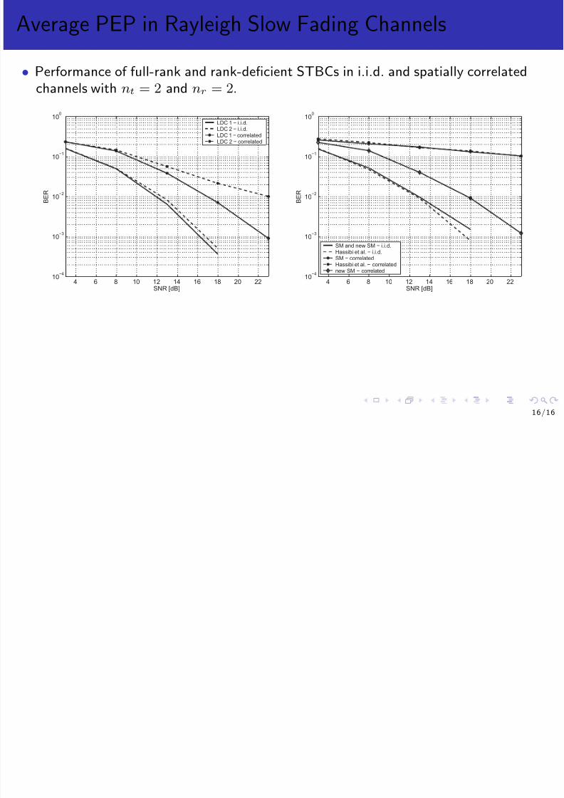
8/12/2019 Wireless Communications Lectures
http://slidepdf.com/reader/full/wireless-communications-lectures 151/271
4 6 8 10 12 14 16 18 20 2210
−4
10−3
10−2
10
SNR [dB]
B E R
4 6 8 10 12 14 16 18 20 2210
−4
10−3
10−2
10
SNR [dB]
B E R
SM and new SM − i.i.d.Hassibi et al. − i.i.d.SM − correlatedHassibi et al. − correlatednew SM − correlated
16/16
Lecture 11: Space-Time Coding with PartialTransmit Channel Knowledge

8/12/2019 Wireless Communications Lectures
http://slidepdf.com/reader/full/wireless-communications-lectures 152/271
Transmit Channel Knowledge
Bruno Clerckx
EE4-65/EE9-SO27 Wireless CommunicationsDepartment of Electrical and Electronic Engineeing
Imperial College London
January 2014
1 / 1 7

8/12/2019 Wireless Communications Lectures
http://slidepdf.com/reader/full/wireless-communications-lectures 153/271
Reference Book
• Bruno Clerckx and Claude Oestges, “MIMO Wireless Networks: Channels,Techniques and Standards for Multi-Antenna, Multi-User and Multi-Cell Systems,”Academic Press (Elsevier), Oxford, UK, Jan 2013.

8/12/2019 Wireless Communications Lectures
http://slidepdf.com/reader/full/wireless-communications-lectures 154/271
– Chapter 10
Section: 10.1, 10.2.1, 10.5, 10.6.1,10.6.2, 10.6.3, 10.6.4, 10.9
3 / 1 7
Introduction
• full CSIT– array and diversity gain– lower system complexity (parallel virtual transmissions)– hardly achievable (especially when the channel varies rapidly), costly in terms of
feedback
• Exploiting Channel Statistics at the Transmitter– low rate feedback link

8/12/2019 Wireless Communications Lectures
http://slidepdf.com/reader/full/wireless-communications-lectures 155/271
low rate feedback link– statistical properties of the channel (correlations, K-factor) vary at a much slower rate
than the fading channel itself – The receiver estimates the channel stochastic properties and sends them back to the
transmitter “once in a while” (if channel reciprocity cannot be exploited)
– stationary channel: statistics do not change over time• Exploiting a Limited Amount of Feedback at the Transmitter– codebook of precoding matrices, i.e., a finite set of precoders, designed off-line and
known to both the transmitter and receiver.– The receiver estimates the best precoder as a function of the current channel and feeds
back only the index of this best precoder in the codebook.
4 / 1 7
System Model
• MIMO system with nt transmit and nr receive antennas communicating through afrequency flat slow fading channel.
• The encoder outputs a codeword C = [c0 . . . cT −1] of size ne × T contained in thecodebook
C over T symbol durations.
• Precoder P [nt ×ne] processes the codeword C and the codeword C′ = PC[nt × T ] is transmitted over nt antennas.

8/12/2019 Wireless Communications Lectures
http://slidepdf.com/reader/full/wireless-communications-lectures 156/271
[ ]
Sconstellation shaper
W
beamformer
P
C’’C C’1/2
• Linear precoder P = WS1/2
– multi-mode beamformer W whose columns have a unit-norm– constellation shaper S1/2 (if S real-valued and diagonal, it can be thought of as the
power allocation scheme across the modes)
• nomalization: E TrC′C′H
= T , E Tr
CCH
= T and Tr
PPH
= ne,
E H2F
= ntnr.
5 / 1 7
Channel Statistics based Precoding
• Information Theory motivated strategy.
Proposition
In Kronecker correlated Rayleigh fast fading channels, the optimal input covariance matrix can again be expressed as

8/12/2019 Wireless Communications Lectures
http://slidepdf.com/reader/full/wireless-communications-lectures 157/271
Q = URtΛQUH Rt
,
where URt is a unitary matrix formed by the eigenvectors of Rt (arranged insuch order that they correspond to decreasing eigenvalues of Rt), and ΛQ is a
diagonal matrix whose elements are also arranged in decreasing order.
Transmit a single stream along the dominant eigenvector of Rt if very large transmitcorrelation. Transmit multiple streams with uniform power allocation if very lowtransmit correltion.
• Error Probability motivated strategy
P⋆ = arg min
PmaxE=0
P (C → E)
– challenging problem for arbitrary codes– focus on O-STBC
6 / 1 7
Channel Statistics based Precoding
• O-STBCs in Kronecker Rayleigh fading channels
P⋆ = arg max
PmaxE=0
detInrnt + ζ R
Inr ⊗PP
H
= arg maxP
maxE=0
detInrnt + ζ Rr ⊗RtPPH
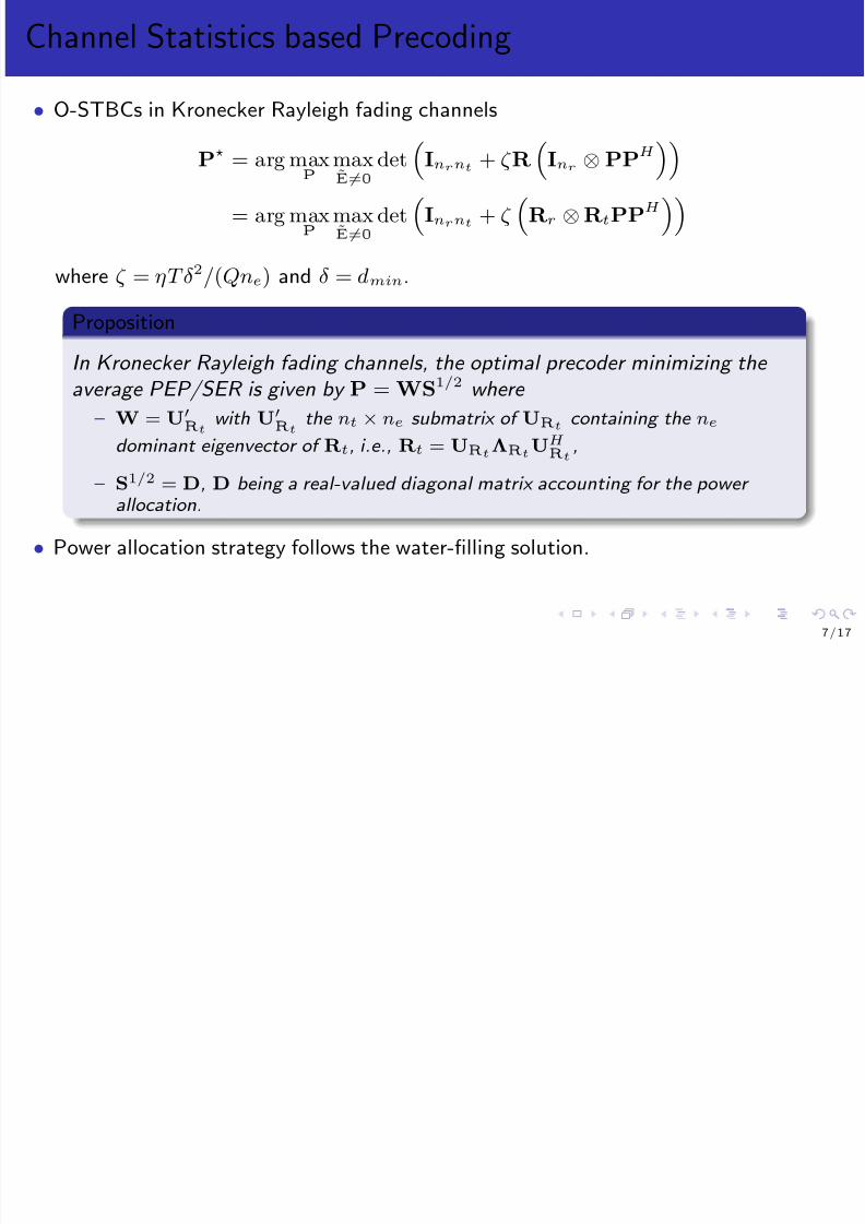
8/12/2019 Wireless Communications Lectures
http://slidepdf.com/reader/full/wireless-communications-lectures 158/271
where ζ = ηT δ 2/(Qne) and δ = dmin.
Proposition
In Kronecker Rayleigh fading channels, the optimal precoder minimizing the average PEP/SER is given by P = WS1/2 where
– W = U′Rt
with U′Rt
the nt × ne submatrix of URt containing the ne
dominant eigenvector of Rt, i.e., Rt = URtΛRt
UH Rt
,
– S1/2 = D, D being a real-valued diagonal matrix accounting for the power
allocation.
• Power allocation strategy follows the water-filling solution.
7 / 1 7
Channel Statistics based Precoding
Example
Let us consider the Alamouti O-STBC with two transmit antennas(ne = nt = 2). Denoting S = diag
s1, s2
, the transmitted codewords are
proportional, at the first time instant, to
1
1 1

8/12/2019 Wireless Communications Lectures
http://slidepdf.com/reader/full/wireless-communications-lectures 159/271
1√ 2URtS
1/2
c1c2
=
1√ 2URt (:, 1)
√ s1c1 +
1√ 2URt (:, 2)
√ s2c2
and, at the second time instant, to
1√ 2URtS
1/2 −c∗2
c∗1
= − 1√
2URt (:, 1)
√ s1c
∗2 +
1√ 2URt (:, 2)
√ s2c
∗1.
Extreme cases:• s1 = s2 = 1: Alamouti scheme
• s1 = 2, s2 = 0: beamforming in the dominant eigenbeamThe precoder allocates more power to angular directions corresponding to thepeaks of the transmit direction power spectrum.
8 / 1 7
Channel Statistics based Precoding
• Performance of a transmit correlation based precoded Alamouti scheme in 2 × 2transmit correlated (t = 0.7 and t = 0.95) Rayleigh channels
10−1
t = 0 .7, Alamoutit = 0 .7, Alamouti with precoder t = 0 .7, single mode eigenbeamformingt = 0 .7, dominant eigenmode transmissioni.i.d., Alamouti
10−1
t = 0 .95,Al amoutit = 0 .95, Alamouti with precoder t = 0 .95, dominant eigenmode transmissioni.i.d., Alamouti

8/12/2019 Wireless Communications Lectures
http://slidepdf.com/reader/full/wireless-communications-lectures 160/271
0 2 4 6 8 10 1210
−3
10−2
SNR [dB]
B E R
0 2 4 6 8 10 12 1410
−3
10−2
SNR [dB]
B E R
9 / 1 7
Quantized Precoding: dominant eigenmode transmission
• Assume dominant eigenmode transmission (i.e. beamforming)
y =√ E sHwc + n,
z = gH y,
= √ E sgH Hwc + gH n
h d i l 1 d 1

8/12/2019 Wireless Communications Lectures
http://slidepdf.com/reader/full/wireless-communications-lectures 161/271
where g and w are respectively nr × 1 and nt × 1 vectors.• Assuming MRC, the optimal beamforming vector w that maximizes the SNR is given
byw⋆ = arg max
w∈Cw Hw
2
with Cw set of unit-norm vectors. The best precoder is the dominant right singularvector of H.
• Reduce the number of feedback bits: limit the space Cw over which w can be chosento a codebook called W . The receiver evaluates the best precoder w⋆ among allunit-norm precoders wi
∈ W (with i = 1, . . . , np) such that
w⋆ = arg max
1≤i≤npwi∈W
Hwi2 .
10/17
Quantized Precoding: distortion function
• How to design the codebook? Need for a distortion function, i.e. measure of theaverage (over all channel realizations) array gain loss induced by the quantizationprocess
df =
E H λmax
− Hw
⋆
2
• Upper-bound

8/12/2019 Wireless Communications Lectures
http://slidepdf.com/reader/full/wireless-communications-lectures 162/271
df ≤ E Hλmax − λmax
vH maxw
⋆2,
(a)
= E H λmax quality of the channel
E H1 − vH
maxw
⋆2
quality of the codebook
where vmax is the dominant right singular vector of H. Equality (a) is only valid fori.i.d. Rayleigh fading channels.
11/17
Quantized Precoding: Lloyd
• Generalized Lloyd Algorithm:
Algorithm
For the given codebook, find the optimal quantization cells using the nearest
neighbor rule. For the so-obtained quantization cells, determine that optimal quantized precoders using the centroid condition. Iterate till convergence.

8/12/2019 Wireless Communications Lectures
http://slidepdf.com/reader/full/wireless-communications-lectures 163/271
• Essential conditions:– Assume MISO channel.– centroid condition: the optimal quantized precoder wk of any quantization cell Rk is
to be chosen as the dominant eigenvector of R
k =
E hH h
|h
∈ Rk
.– nearest neighbor rule : all channel vectors that are closer to the quantized precoder wkare assigned to quantization cell Rk, i.e. h ∈ Rk if
h2 − h2 hwk
2 ≤ h2 − h2hwj
2,
• Optimal codebook design for arbitrary fading channels
12/17
Quantized Precoding: Grassmannian
• Grassmannian Line Packing
Design Criterion
Choose a codebook W
made of np
unit-norm vectors wi (i = 1, . . . , n
p) such
that the minimum distance 2

8/12/2019 Wireless Communications Lectures
http://slidepdf.com/reader/full/wireless-communications-lectures 164/271
δ line (W ) = min1≤k<l≤np
1 − |wH
k wl|2,
is maximized.
– Problem of packing np lines in
nt insuch a way that the minimum distancebetween any pair of lines is maximized.
– Close to optimal only for i.i.d. Rayleigh
Fading Channels.
13/17
Quantized Precoding: How many bits?
• How many feedback bits B = log2 (np) are required? In i.i.d. channels
C quant ≈ E h
log2
1 + ρ h2
1 − 2
− Bnt−1
,
leading to an SNR degradation of 10 log101 − 2− Bnt−1 dB relative to perfect
CSIT.

8/12/2019 Wireless Communications Lectures
http://slidepdf.com/reader/full/wireless-communications-lectures 165/271
Proposition
In order to maintain a constant SNR or capacity gap between perfect CSIT and
quantized feedback, it is not necessary to scale the number of feedback bits as a function of the SNR. The multiplexing gain gs is not affected by the quality of CSIT.
• Achievable diversity gain?– Antenna selection (AS) is a particular case of a quantized precoding whose codebook is
chosen as the columns of the identity matrix Int
.– AS achieves a diversity gain of nt.– Sufficient to take a full rank codebook matrix with np ≥ nt to extract the full diversity
14/17
Quantized Precoding: Evaluations
• SER of a 3 × 3 MIMO system using 2-bit and 6-bit quantized BPSK-based DET.
10−3
10−2
2-bit D-DET6-bit Q-DET
ant. selectionP-DET
Example
Codebook for quantized DET fornt = 3 and np = 4.
1
j

8/12/2019 Wireless Communications Lectures
http://slidepdf.com/reader/full/wireless-communications-lectures 166/271
0 1 2 3 4 5 6
10−4
SNR [dB]
S E R
W =
1√ 31√ 31√ 3
,
j√ 3−1√ 3−j√ 3
,
−1√ 31√ 3−1√ 3
,
−j√ 3−1√ 3j√ 3
15/17
Quantized Precoding: spatially correlated channels
• Grassmiannian only appropriate for i.i.d. Rayleigh fading.• Spatial correlation decreases the quantization space compared to i.i.d. channels.
– e.g. Lloyd, adaptive/CDIT-based codebook, DFT (for uniform linear arrays)
• Normalized average distortion (SNR loss) df,n = df /
E H
λmax
as a function of the
codebook size np = 2B and the transmit correlation coefficient t with nt = 4.
0.4

8/12/2019 Wireless Communications Lectures
http://slidepdf.com/reader/full/wireless-communications-lectures 167/271
0 0.1 0.2 0.3 0.4 0.5 0.6 0.7 0.8 0.9 10
0.05
0.1
0.15
0.2
0.25
0.3
0.35
Magnitude of the transmit correlation coefficient t
A v e r a g e
d i s t o r t i o n
d f , n
CDIT−based CB, B=3CDIT−based CB, B=4
CDIT−based CB, B=5
|t|−based CB, B=4
DFT CB, B=4GLP CB, B=4
16/17
Quantized Precoding: some extensions
• Extension to other kinds of channel models (e.g. spatial/time correlation,polarization), transmission strategies (e.g. O-STBCs, SM), reception strategies (e.g.MRC, ZF, MMSE, ML), criteria (e.g. error rate or transmission rate)
• Quantized precoding for SM with rank adaptation and rate maximization
W⋆ = arg max
nemax
W(ne)i ∈W ne
R.
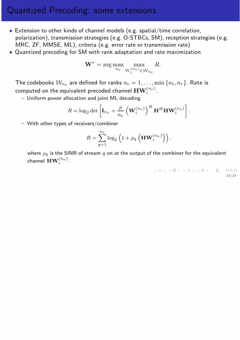
8/12/2019 Wireless Communications Lectures
http://slidepdf.com/reader/full/wireless-communications-lectures 168/271
The codebooks W ne are defined for ranks ne = 1, . . . ,min nt, nr. Rate is
computed on the equivalent precoded channel HW(ne)i .
– Uniform power allocation and joint ML decoding
R = log2 det
Ine +
ρ
ne
W
(ne)i
H HH HW
(ne)i
.
– With other types of receivers/combiner
R =
ne
q=1
log2 1 + ρq HW(ne)i .
where ρq is the SINR of stream q on at the output of the combiner for the equivalent
channel HW(ne)i .
17/17
Lecture 12: Frequency-Selective MIMO Channels- MIMO-OFDM

8/12/2019 Wireless Communications Lectures
http://slidepdf.com/reader/full/wireless-communications-lectures 169/271
Bruno Clerckx
EE4-65/EE9-SO27 Wireless CommunicationsDepartment of Electrical and Electronic Engineeing
Imperial College London
January 2014
1 / 1 8
Contents
1 Introduction
2 Single-Carrier Transmissions

8/12/2019 Wireless Communications Lectures
http://slidepdf.com/reader/full/wireless-communications-lectures 170/271
3 Multi-Carrier Transmissions: MIMO-OFDM
4 Unified Representation for Single and Multi-Carrier Transmissions
5 Code Design for Single-Carrier Transmissions
6 Code Design for Space-Frequency Coded MIMO-OFDM
2 / 1 8
Reference Book
• Bruno Clerckx and Claude Oestges, “MIMO Wireless Networks: Channels,Techniques and Standards for Multi-Antenna, Multi-User and Multi-Cell Systems,”Academic Press (Elsevier), Oxford, UK, Jan 2013.

8/12/2019 Wireless Communications Lectures
http://slidepdf.com/reader/full/wireless-communications-lectures 171/271
– Chapter 11
Section: 11.1, 11.4.1, 11.5.2
3 / 1 8
Introduction
• Two major different approaches to transmit information over frequency selectiveMIMO channels:
– modulating a single carrier over the full bandwidth B.– converts the frequency selective channel into a set of multiple parallel flat fading
channels in the frequency domain by means of Orthogonal Frequency Division
Multiplexing (OFDM) modulation.
8/12/2019 Wireless Communications Lectures
http://slidepdf.com/reader/full/wireless-communications-lectures 172/271
4 / 1 8
Single-Carrier Transmissions
• Transmission of a codeword C = [c0 . . . cT −1] (of size nt × T )• Presence of L resolvable taps, which are responsible for inter-symbol interference
(ISI)
H[τ ] =
L−1
l=0
H[l]δ (τ − τ l)
– L replicas of the same codeword → Lth order diversity!

8/12/2019 Wireless Communications Lectures
http://slidepdf.com/reader/full/wireless-communications-lectures 173/271
L replicas of the same codeword → L order diversity!
• How to design codewords such that a ML decoder is able to efficiently exploit thefrequency and spatial diversity without suffering from the ISI?
• System model
yk =√
E s
L−1l=0
H [l] ck−l + nk
where yk, nk, E s are defined analogous to frequency flat fading channels.
5 / 1 8
Virtual Transmit Antenna Array
• Equivalent system model
yk =√
E sH
cT k . . . cT k−L+1
T + nk
H H [0] . . . H [L
− 1]
– L taps may be thought of as virtual transmit antennasVirtual transmit array of n L antennas where the n × n L virtual channel matrix is H

8/12/2019 Wireless Communications Lectures
http://slidepdf.com/reader/full/wireless-communications-lectures 174/271
– Virtual transmit array of ntL antennas where the nr × ntL virtual channel matrix is Hand equivalent codeword
C =
c0 c1 . . . cT −1
c−1
c0
. . . cT −
2......
. . ....
c1−L c2−L . . . cT −L
– Maximum diversity gain of nrntL
6 / 1 8
Multi-Carrier Transmissions: MIMO-OFDM
• Frequency domain approach to exploit the frequency diversity
• Basic idea of OFDM: Turn the channel matrix into a circulant matrix via theaddition of a cyclic prefix to the transmitted sequence
– A circulant matrix has the property that its left and right singular vector matrices arerespectively DFT and IDFT matrices.– The multiplication by an IDFT matrix at the transceiver and by a DFT matrix at the
receiver transforms the frequency selective channel into a diagonal matrix, whose
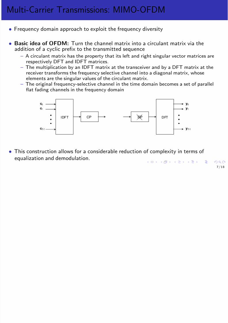
8/12/2019 Wireless Communications Lectures
http://slidepdf.com/reader/full/wireless-communications-lectures 175/271
receiver transforms the frequency selective channel into a diagonal matrix, whoseelements are the singular values of the circulant matrix.
– The original frequency-selective channel in the time domain becomes a set of parallelflat fading channels in the frequency domain
PIDFT DFT•
•
•
•
•
•
c0
c1
cT -1
y0
y1
yT -1
CP CP
• This construction allows for a considerable reduction of complexity in terms of equalization and demodulation.
7 / 1 8
Orthogonal Frequency Division Multiplexing (OFDM)
• Fundamental Steps 1 to 6
1 Apply an IDFT to the codeword C. We obtain as output at the nth time interval(n = 0, . . . , T − 1),
xn = 1√ T
T −1k=0
ckej 2π
T
kn
,
or equivalently in a matrix form,

8/12/2019 Wireless Communications Lectures
http://slidepdf.com/reader/full/wireless-communications-lectures 176/271
x0 . . . xT −1
T = DH
c0 . . . cT −1
T ,
xT 0 . . . xT
T −1 T = DH
⊗Int cT 0 . . . cT T −1 T .
The T × T matrix DH realizes the IDFT operation. Hence, D is a DFT matrixreading as
D = 1√ T
1 1 1 . . . 1
1 e−j 2π
T e−j 2π
T 2 . . . e−j
2π
T (T −1)
... . . . ... ... ...
1 e−j 2π
T (T −2) e−j
2π
T (T −2)2 . . . e−j
2π
T (T −2)(T −1)
1 e−j 2π
T (T −1) e−j
2π
T (T −1)2 . . . e−j
2π
T (T −1)(T −1)
.
8 / 1 8
Orthogonal Frequency Division Multiplexing (OFDM)
2 Add the guard interval vector Xg =
x−(L−1) . . . x−1
of length L − 1 in front of
the codeword X = [ x0 . . . xT −1 ] to avoid inter-symbol interference.Choose the guard interval vector Xg in such way that x−n = xT −n, forn = 1, . . . , L − 1. Hence, the guard interval vector becomes
Xg =
xT −(L−1) . . . xT −1
and is commonly known as the cyclic prefix.3 Transmit the OFDM symbol X′ =
Xg X
of size nt × (T + L − 1).
4 Remove the guard interval (CP) at the receiver and gather T output samples as

8/12/2019 Wireless Communications Lectures
http://slidepdf.com/reader/full/wireless-communications-lectures 177/271
rT 0 . . . rT T −1
T = Hg
xT −(L−1) . . . xT
T −1
T +
nT 0 . . . nT
T −1
T
where
Hg =
H [L − 1] . . . H [1] H [0] 0nr×nt . . . 0nr×nt
0nr×nt H [L − 1]. . . H [1] H [0] . . . 0nr×nt
.... . .
. . . . . .
. . . . . .
...
0nr×
nt . . . 0nr×
nt H [L − 1] H [L − 2] . . . H [0]
is a nrT ×nt(T + L − 1) matrix representing the channel seen by the OFDM symbol.
9 / 1 8
Orthogonal Frequency Division Multiplexing (OFDM)
5 Observe that the choice of the CP creates a blockwise circulant matrix Hcp of sizenrT × ntT
rT 0 . . . rT T −1T
= Hcp
xT
0 . . . xT T −1
T +
nT 0 . . . nT
T −1
T with
H [0] 0nr×nt . . . 0nr×nt H [L− 1] . . . H [1]H [1] H [0] 0nr×nt . . . 0nr×nt . . . H [2]
. . . . . . .
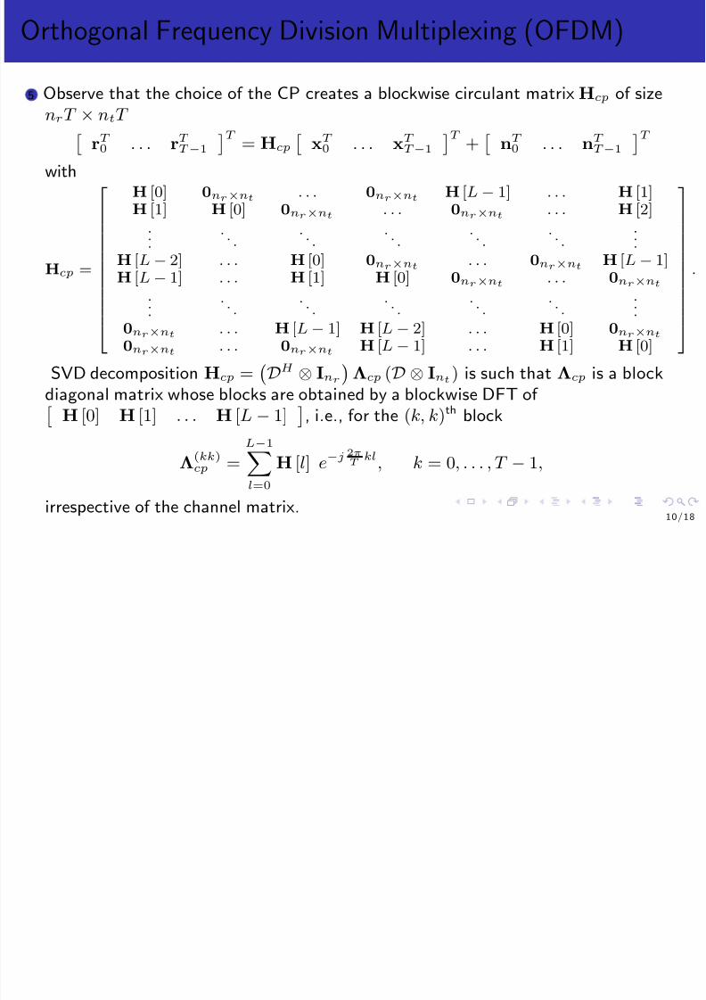
8/12/2019 Wireless Communications Lectures
http://slidepdf.com/reader/full/wireless-communications-lectures 178/271
Hcp =
.. . . . . . . . . . . ..H [L− 2] . . . H [0] 0nr×nt . . . 0nr×nt H [L− 1]H [L− 1] . . . H [1] H [0] 0nr×nt . . . 0nr×nt
... . . . . . . . . . . . . . . . ...0nr×nt . . . H [L− 1] H [L − 2] . . . H [0] 0nr×nt0nr×nt . . . 0nr×nt H [L − 1] . . . H [1] H [0]
.
SVD decomposition Hcp =DH ⊗ Inr
Λcp (D ⊗ Int) is such that Λcp is a block
diagonal matrix whose blocks are obtained by a blockwise DFT of
H [0] H [1] . . . H [L − 1]
, i.e., for the (k, k)
th
block
Λ(kk)cp =
L−1l=0
H [l] e−j 2π
T kl
, k = 0, . . . , T − 1,
irrespective of the channel matrix.10/18
8/12/2019 Wireless Communications Lectures
http://slidepdf.com/reader/full/wireless-communications-lectures 179/271
Orthogonal Frequency Division Multiplexing (OFDM)
• MIMO-OFDM System Model: The input-output relationship on each parallelchannel k = 0, . . . , T − 1 may be expressed without loss of generality as
yk =√
E sH(k)ck + nk
with
H(k) = Λ(kk)cp =
L−1l 0
H [l] e−j 2π
T kl
.

8/12/2019 Wireless Communications Lectures
http://slidepdf.com/reader/full/wireless-communications-lectures 180/271
l=0
The nr × 1 vector yk is the received signal to be decoded, and nk is a nr × 1 zeromean complex AWGN vector with
EnknH
k′
= σ2
nInrδ [k
− k′].
• If ML decoding is applied, the decoder computes an estimate of the transmittedcodeword according to
C = arg minC
T −1k=0
yk −√
E sH(k)ck
2
.
12/18
Orthogonal Frequency Division Multiplexing (OFDM)
• Block diagram of a MIMO-OFDM system
encoder
S/ P
S/ P
interleaver OFDM
modulator
interleaver OFDM
modulator

8/12/2019 Wireless Communications Lectures
http://slidepdf.com/reader/full/wireless-communications-lectures 181/271
decoder interleaver de- OFDM
demodulator
• Strong analogy with the input-output relationship over a flat fading MIMO channel:– Temporal dimension replaced by frequency dimension– Hk ↔H(k)
– Commonly known as Space-Frequency Coded MIMO-OFDM.– If the coherence bandwidth of the channel is small, the channel gains H(k) vary
significantly from tone to tone. The channel in the frequency domain can then beconsidered as a fast fading channel in the frequency domain.
13/18
Virtual Transmit Antenna Array
• Virtual transmit array
yk =√
E sH
cT k . . . e−j 2π
T klcT k . . . e−j
2π
T k(L−1)cT k
T + nk
where H is the nr × ntL virtual channel matrix and the equivalent codeword is c0 . . . ck . . . cT −1
. . . . .

8/12/2019 Wireless Communications Lectures
http://slidepdf.com/reader/full/wireless-communications-lectures 182/271
C =
.. . . .. .. ..
e−j 2π
T klck
.
.....
.
...
. ....
c0 . . . e−j 2π
T k(L−1)ck . . . e−j
2π
T (T −1)(L−1)cT −1
• Equivalent codewords differ from the single-carrier case.• Maximum diversity gain of nrntL.
14/18
Unified Representation for Single and Multi-Carrier
Transmissions• Unique virtual nr × Lnt MIMO channel
Y =
y0 · · · yT −1
=
√ E sH C +
n0 · · · nT −1
• Equivalent transmitted codewords in the virtual nr × Lnt MIMO representation
C =
C(0)
...C(L 1)

8/12/2019 Wireless Communications Lectures
http://slidepdf.com/reader/full/wireless-communications-lectures 183/271
C(L−1)
– Space-frequency coded MIMO-OFDM
C(0)
...C(L−1)
=
CD(0)
...CD(L−1)
= [IL ⊗C]
D(0)
...D(L−1)
D
with D(l) = diag 1, . . . , e−j 2π
T kl, . . . , e
−j 2π
T (T −1)l
.
– Single carrier transmissions,
C(l) (m, k) = ck−l (m, 1) , k = 0, . . . , T − 1, m = 1, . . . , nt.
• Maximum-likelihood (ML) decoding: C = arg minCY − √
E sH C2
15/18
Code Design for Single-Carrier Transmissions
Example
Send c0, . . . , cT −1 over two antennas in a 2-tap Rayleigh fading channel.• classical delay-diversity scheme
C = 1√
2
c0 c1 . . . cT −1 0 0
0 c0 c1 . . . cT −1 0
,
Diversity of

8/12/2019 Wireless Communications Lectures
http://slidepdf.com/reader/full/wireless-communications-lectures 184/271
C = 1
√ 2
c0 c1 . . . cT −1 0 00 c0 c1 . . . cT −1 00 c0 c1 . . . cT −1 00 0 c0 c1 . . . cT −1
.
Diversity of 3nr only!
• Generalized delay-diversity scheme
C = 1√
2
c0 c1 . . . cT −1 0 0 0
0 0 c0 c1 . . . cT −1 0
,
C = 1√
2
c0 c1 . . . cT −1 0 0 00 0 c0 c1 . . . cT −1 00 c0 c1 . . . cT −1 0 00 0 0 c0 c1 . . . cT −1
.
Diversity of 4nr!
16/18
Code Design for Space-Frequency Coded MIMO-OFDM
• MIMO-OFDM ≈ narrowband MIMO transmissions over i.i.d. fast fading Rayleighchannels if L >> 0.
Example
SISO channel h(k) = L−1
l=0 h [l] e−j 2π
T
kl
. Frequency correlation betweenchannel on subcarrier k and k + K
L−1 | [ ]|2 2π lK

8/12/2019 Wireless Communications Lectures
http://slidepdf.com/reader/full/wireless-communications-lectures 185/271
E h(k)h(k+K)∗
=l=0
E |h[l]|2 e T lK
Frequency correlation reduces the achievable coding gain. Reduce the frequencycorrelation between adjacent tones by means of an interleaver.
• Space-Frequency Linear Block Coding– Orthogonal codes: O-STBC → O-SFBC (time replaced by frequency)– Make sure that O-SFBC is operated on adjacent subcarriers. Recall that the channel
has to be constant within a O-STBC/O-SFBC block!
– In practice, O-SFBC often preferred over O-STBC.
17/18
Code Design for Space-Frequency Coded MIMO-OFDM
• With interleaver, use codes with large effective length and product distance forOFDM transmissions as in fast fading channels.
• FER of the 16-state space-time trellis code for L = 2, 3 and 4 in uniformlydistributed i.i.d. Rayleigh channels with and without interleaver.
100

8/12/2019 Wireless Communications Lectures
http://slidepdf.com/reader/full/wireless-communications-lectures 186/271
7.5 10 12.5 15 17.5
10−3
10−2
10−1
SNR [dB]
F E R
L=2, with interleaver
L=3, with interleaver
L=4, with interleaver
fast fading
L=2, no interleaver
L=3, no interleaver L=4, no interleaver
18/18
Lecture 13&14: Multi-User MIMO - Multiple
Access Channels (Uplink) & Broadcast Channels(Downlink)

8/12/2019 Wireless Communications Lectures
http://slidepdf.com/reader/full/wireless-communications-lectures 187/271
Bruno Clerckx
EE4-65/EE9-SO27 Wireless CommunicationsDepartment of Electrical and Electronic Engineeing
Imperial College London
January 2014
1 / 2 4
Contents
1 Introduction
2 MIMO MAC System Model
3 Capacity Region of Deterministic ChannelsCapacity Region of MIMO MACAchievability of the Capacity Region

8/12/2019 Wireless Communications Lectures
http://slidepdf.com/reader/full/wireless-communications-lectures 188/271
Achievability of the Capacity RegionComparisons with TDMA
4 MIMO BC System Model
5 Capacity Region of Deterministic ChannelsCapacity Region of SISO BCAchievability of the SISO BC Capacity Region
Capacity Region of MIMO BC and its AchievabilityComparisons with TDMA
2 / 2 4
Reference Book
• Bruno Clerckx and Claude Oestges, “MIMO Wireless Networks: Channels,Techniques and Standards for Multi-Antenna, Multi-User and Multi-Cell Systems,”Academic Press (Elsevier), Oxford, UK, Jan 2013.

8/12/2019 Wireless Communications Lectures
http://slidepdf.com/reader/full/wireless-communications-lectures 189/271
– Chapter 12
Section: 12.1, 12.2, 12.3
3 / 2 4
Introduction
• So far, we looked at a single link/user. Most systems are multi-user!• How to deal with multiple users? What is the benefit of MIMO in a multi-user
setting?• MIMO Broadcast Channel (BC) and Multiple Access Channel(MAC)

8/12/2019 Wireless Communications Lectures
http://slidepdf.com/reader/full/wireless-communications-lectures 190/271
Differences between BC and MAC:– there are multiple independent receivers (and therefore multiple independent additive
noises) in BC while there is a single receiver (and therefore a single noise term) in MAC.– there is a single transmitter (and therefore a single transmit power constraint) in BC
while there are multiple transmitters (and therefore multiple transmit powerconstraints) in MAC.
– the desired signal and the interference (originating from the co-scheduled signals)propagate through the same channel in the BC while they propagate through differentchannels in the MAC.
4 / 2 4

8/12/2019 Wireless Communications Lectures
http://slidepdf.com/reader/full/wireless-communications-lectures 191/271
MIMO MAC System Model
• By stacking up the transmit signal vectors and the channel matrices of all K users,
c′
ul =c′T ul,1, . . . , c
′T ul,K
T ,
Hul
= Λ−1/2
1 H
ul,1, . . . , Λ
−1/2
K H
ul,K ,
the system model also writes as
yul = Hulc′l + nul

8/12/2019 Wireless Communications Lectures
http://slidepdf.com/reader/full/wireless-communications-lectures 192/271
yul = Hulcul + nul.
Hul is assumed to be full-rank as it would be the case in a typical user deployment.
• Long term SNR of user q defined as ηq = E s,qΛ−1q /σ2
n.
• Note on the notations: the dependence on the path loss and shadowing is madeexplicit in order to stress that the co-scheduled users experience different path lossesand shadowings and therefore receive power.
• We assume that the receiver (i.e. the BS in a UL scenario) has always perfectknowledge of the CSI, but we will consider strategies where the transmitters haveperfect or partial knowledge of the CSI.
6 / 2 4
Capacity Region of Deterministic Channels
• In a multi-user setup, given that all users share the same spectrum, the rateachievable by a given user q , denoted as Rq, will depend on the rate of the otherusers Rp, p = q → Trade-off between rates achievable by different users!
• The capacity region C formulates this trade-off by expressing the set of all user rates
(R1, . . . , RK) that are simultaneously achievable.Definition
The capacity region C of a channel H is the set of all rate vectors

8/12/2019 Wireless Communications Lectures
http://slidepdf.com/reader/full/wireless-communications-lectures 193/271
p y g(R1, . . . , RK) such that simultaneously user 1 to user K can reliablycommunicate at rate R1 to rate RK , respectively.
Any rate vector not in the capacity region is not achievable (i.e. transmission atthose rates will lead to errors).
Definition
The sum-rate capacity C of a capacity region C is the maximum achievablesum of rates
C = max(R1,...,RK)∈C
Kq=1
Rq.
7 / 2 4
Rate Region of MIMO MAC
• For given input covariance matrices Qul,1, . . . ,Qul,K , the achievable rate region isdefined by
1 The rate achievable by a given user q with a given transmit strategy Qul,q cannot belarger than its achievable rate in a single-user setup, i.e.
Rq ≤ log2 detInr +
Λ−1q
σ2n Hul,qQul,qH
H ul,q
, q = 1, . . . , K
where Qul,q = E c′qc
′qH is subject to the power constraint TrQul,q ≤ E s,q.
2 The sum of the rates achievable by a subset S of the users should be smaller than thetotal rate achievable when those users “cooperate” with each other to form a giant

8/12/2019 Wireless Communications Lectures
http://slidepdf.com/reader/full/wireless-communications-lectures 194/271
total rate achievable when those users cooperate with each other to form a giantarray with nt,S =
q∈S nt,q transmit antennas subject to their respective power
constraints, i.e.q∈S
Rq ≤ log2 detInr +
1
σ2n
Hul,SQul,SHH ul,S
= log2 det
Inr +
1
σ2n
q∈S
Λ−1q Hul,qQul,qH
H ul,q
,
with Hul,S =
Λ
−1/2
i Hul,i, . . . , Λ
−1/2
j Hul,ji,j∈S ,
Qul,S = diagQul,i, . . . ,Qul,j
i,j∈S
, subject to the constraints TrQul,q ≤ E s,q.
• The rate region looks like a K -dimensional polyhedron with K ! corner points on theboundary.
8 / 2 4
Rate Region of a Two-User MIMO MAC
• This rate region is a pentagon with two corner points A and B.

8/12/2019 Wireless Communications Lectures
http://slidepdf.com/reader/full/wireless-communications-lectures 195/271
• Remarkably, at point A, user 1 can transmit at a rate equal to its single-link MIMOrate and user 2 can simultaneously transmit at a rate R′
2 > 0 equal to
R′2 = log2 det
Inr +
Λ−11
σ2nHul,1Qul,1H
H ul,1 +
Λ−12
σ2nHul,2Qul,2H
H ul,2
− log2 detInr +
Λ−11
σ2n
Hul,1
Qul,1
HH
ul,1
= log2 det
Inr +
Λ−12
σ2nHul,2Qul,2H
H ul,2
Inr +
Λ−11
σ2n
Hul,1Qul,1HH ul,1
−1 .
9 / 2 4
Capacity Region of MIMO MAC
• We have assumed so far specific input covariance matrices.– A different choice of the beamforming matrix and the power allocation leads to a
different transmit strategy Qul,q and generally a different shape of the pentagon (ormore generally the K -dimensional polyhedron).
– The trade-off between user rates is therefore affected by the choice of the input
covariance matrices.– The optimal set of input covariance matrices that maximizes the sum-rate can be foundusing a generalization of the single-link water-filling solution (Detail in the book).
• The capacity region is equal to the union (over all transmit strategies satisfying thepower constraints) of all the K dimensional polyhedrons
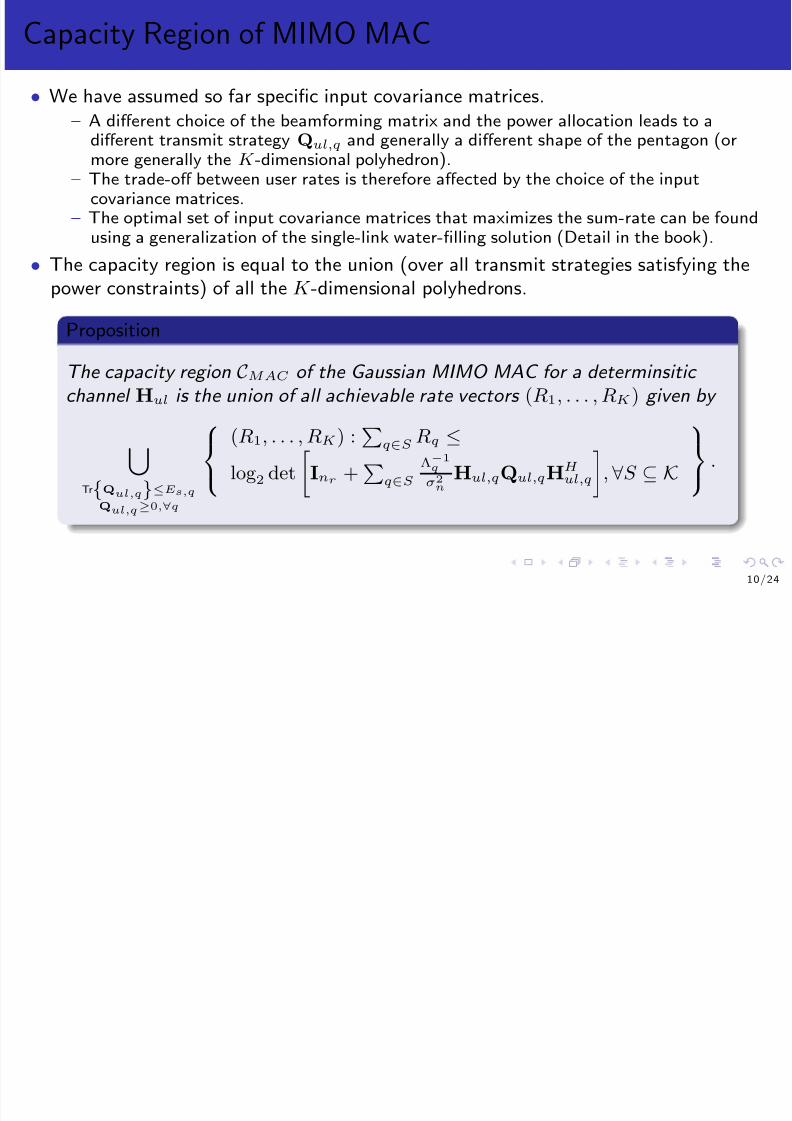
8/12/2019 Wireless Communications Lectures
http://slidepdf.com/reader/full/wireless-communications-lectures 196/271
power constraints) of all the K -dimensional polyhedrons.
Proposition
The capacity region C MAC of the Gaussian MIMO MAC for a determinsitic channel Hul is the union of all achievable rate vectors (R1, . . . , RK) given by
TrQul,q≤Es,qQul,q≥0,∀q
(R1, . . . , RK) :
q∈S Rq ≤
log2 detInr +
q∈S
Λ−1q
σ2n Hul,qQul,qH
H
ul,q
, ∀S ⊆ K .
10/24
Capacity Region of a Two-User MIMO MAC
• Due to the union of pentagons, the capacity region of the two-user MIMO MACdoes not look like a pentagon in general.

8/12/2019 Wireless Communications Lectures
http://slidepdf.com/reader/full/wireless-communications-lectures 197/271
• However, with a single antenna (nt,q = 1), the capacity region remains a pentagonbecause a single data is transmitted per user at the full power, i.e. E s,q.
11/24
Capacity Region of SISO MAC
Corollary
C MAC = (R1, . . . , RK) :q∈S
Rq ≤ log2 1 +q∈S
ηq |hul,q|2 , ∀S ⊆ Kwhere ηq = Λ−1
q E s,q/σ2n.
Example

8/12/2019 Wireless Communications Lectures
http://slidepdf.com/reader/full/wireless-communications-lectures 198/271
Example
Two-user SISO: C MAC is the set of all rates pair (R1, R2) satisfying to
Rq ≤ log2
1 + ηq |hul,q |2
, q = 1, 2
R1 + R2 ≤ log2
1 + η1 |hul,1|2 + η2 |hul,2|2
.
R′2 = log2 1 + η1 |hul,1|2 + η2 |hul,2|2− log2 1 + η1 |hul,1|2
= log2
1 +
η2 |hul,2|2
1 + η1 |hul,1|2
= log2
1 +
Λ−12 |hul,2|2 E s,2
σ2n + Λ−1
1 |hul,1|2 E s,1
.
12/24
Capacity Region of SIMO MAC
Corollary
C MAC =
(R1, . . . , RK) :
q∈S Rq ≤
log2 det Inr +q∈S ηqhul,qhH ul,q , ∀S ⊆ K
where ηq = Λ−1q E s,q/σ2
n.
Example

8/12/2019 Wireless Communications Lectures
http://slidepdf.com/reader/full/wireless-communications-lectures 199/271
Two-user SIMO: C MAC is the set of all rates pair (R1, R2) satisfying to
Rq ≤ log2
1 + ηq hul,q2
= log2 detInr + ηqhul,qh
H ul,q
, q = 1, 2
R1 + R2 ≤ log2 detInr + η1hul,1h
H ul,1 + η2hul,2h
H ul,2
.
R
′
2 = log2 detInr + η1hul,1h
H
ul,1 + η2hul,2h
H
ul,2
− log2 detInr + η1hul,1h
H
ul,1
= log2 detInr + η2hul,2h
H ul,2
Inr + η1hul,1h
H ul,1
−1 = log2
1 + η2h
H ul,2
Inr + η1hul,1h
H ul,1
−1
hul,2
13/24
Achievability of the Capacity Region
• For nt = 1, the SIMO MAC architecture is reminiscent of the Spatial Multiplexingarchitecture discussed for a single-link MIMO channel.
• We can therefore fully reuse the various receiver architectures derived for single-linkMIMO.
• Recall the optimality of the MMSE V-BLAST (also called Spatial Multiplexing withMMSE-SIC receiver)
Proposition
MMSE-SIC is optimal for achieving the corner points of the MIMO MAC rate

8/12/2019 Wireless Communications Lectures
http://slidepdf.com/reader/full/wireless-communications-lectures 200/271
MMSE SIC is optimal for achieving the corner points of the MIMO MAC rate region.
• The exact corner point that is achieved on the rate region depends on the streamcancellation ordering:
– Point A, user 2 is canceled first (i.e. all streams from user 2) such that user 1 is leftwith the Gaussian noise and can achieve a rate equal to the single-link bound.
– Assuming nt = 1, R′2 = log2(1 + ρq) where ρq is the SINR of the MMSE receiver for
user 2’s stream treating user 1’s stream as colored Gaussian interference.
14/24
Comparisons with TDMA
• TDMA allocates the time resources in an orthogonal manner such that users arenever transmitting at the same time (line D-C in the rate region).
• SISO: both TDMA and SIC exploit a single degree of freedom but TDMA rateregion is strictly smaller than the one achievable with SIC.
• SIMO: TDMA incurs a big loss compared to SIMO MAC (with MMSE-SIC) as itonly exploits a single degree of freedom despite the presence of min nr, K degreesof freedom achievable with SIMO MAC at high SNR.

8/12/2019 Wireless Communications Lectures
http://slidepdf.com/reader/full/wireless-communications-lectures 201/271
• MIMO: As nt increases, the gap between the TDMA and MIMO MAC rate regions
decreases.
15/24

8/12/2019 Wireless Communications Lectures
http://slidepdf.com/reader/full/wireless-communications-lectures 202/271
MIMO BC System Model
• By stacking up the received signal vectors, the noise vectors and the channelmatrices of all K users,
y =
yT 1 , . . . ,yT K
T
,
n =nT 1 , . . . ,nT KT
,
H =
Λ−1/21 H
T 1 , . . . , Λ
−1/2K H
T K
T ,
the system model also writes as

8/12/2019 Wireless Communications Lectures
http://slidepdf.com/reader/full/wireless-communications-lectures 203/271
the system model also writes as
y = Hc′ + n.
H is assumed to be full-rank as it would be the case in a typical user deployment.• SNR of user q defined as ηq = E sΛ−1
q /σ2n,q.
• Perfect instantaneous channel state information (CSI) at the Tx and all Rx.• Generally speaking, c′ is written as the superposition of statistically independent
signals c′q
c′ =
Kq=1
c′
q.
The input covariance matrix of user q is defined as Qq = E c′qc
′H q
.
17/24
Capacity Region of two-user SISO Deterministic BC
• In two-user SISO MAC, point A was obtained by canceling user 2’s signal first suchthat user 1 is left with Gaussian noise.
• Let us apply the same philosophy to the SISO BC:– transmit c′ = c′1 + c′2, with power of c′q denoted as sq– user 1 cancels user 2’s signal c′2 so as to be left with its own Gaussian noise
– user 2 decodes its signal by treating user 1’s signal c′1 as Gaussian noise.• Achievable rates of such strategy (with sum-power constraint s1 + s2 = E s)
R1 = log2
1 +
Λ−11 s1
σ2n,1
|h1|2

8/12/2019 Wireless Communications Lectures
http://slidepdf.com/reader/full/wireless-communications-lectures 204/271
n,1
R2 = log2
1 +
Λ−12 |h2|2 s2
σ2n,2 + Λ−1
2 |h2|2 s1
.
• Careful! For user 1 to be able to correctly cancel user 2’s signal, user 1’s channel hasto be good enough to support R2, i.e.
R2 ≤ log21 + Λ−1
1 |h1|2 s2
σ2
n,1 + Λ−1
1 |h1|
2
s1 .
• The channel gains normalized w.r.t. their respective noise power should be ordered
Λ−12 |h2|2
σ2n,2
≤ Λ−1
1 |h1|2
σ2n,1
.18/24
Capacity Region of two-user SISO Deterministic BC
• If the ordering condition is satisfied, the above strategy achieves the boundary of thecapacity region of the two-user SISO BC for any power allocation s1 and s2satisfying s1 + s2 = E s.
• The capacity region is given by the union of all rate pairs (R1, R2) over all powerallocations s1 and s2 satisfying s1 + s2 = E s.

8/12/2019 Wireless Communications Lectures
http://slidepdf.com/reader/full/wireless-communications-lectures 205/271
19/24
Capacity Region of K-user SISO Deterministic BC
• Define hq = Λ−1/2q hq/σn,q. Assume |h1|2 ≥ |h2|2 ≥ . . . ≥ |hK|2.
Proposition
With the ordering |h1|2 ≥ |h2|2 ≥ . . . ≥ |hK|2, the capacity region C BC of the
Gaussian SISO BC is the set of all achievable rate vectors (R1, . . . , RK) givenby
(R1, . . . , RK) : Rq ≤ log2
1 +
|hq|2 sq2 1
, ∀q
.

8/12/2019 Wireless Communications Lectures
http://slidepdf.com/reader/full/wireless-communications-lectures 206/271
sq :Kq=1
sq=Es
( , , ) q g2
1 + |hq|2 q−1p=1 sp
, q
Proposition
The sum-rate capacity of the SISO BC is achieved by allocating the transmit power to the strongest user
C BC = log2
1 + E s maxq=1,...,K |hq|2
= log2
1 + maxq=1,...,K ηq |hq|2
.
Recall that the MAC sum-rate capacity is obtained with all users simultaneouslytransmitting at their respective full power.
20/24
Achievability of the SISO BC Capacity Region
• Receiver cancellation - Superposition coding with SIC and appropriate ordering :– User ordering: decode and cancel out weaker users signals before decoding their own
signal.– The weakest user decodes only the coarsest constellation. The strongest user decodes
and subtracts all constellation points in order to decode the finest constellation.
• Transmitter cancellation - Dirty-Paper Coding (DPC)– Assume a system model y = hc′ + i + n with i, n Gaussian interference and noise.Simply subtracting i for transmit signal is not a good idea!
Proposition

8/12/2019 Wireless Communications Lectures
http://slidepdf.com/reader/full/wireless-communications-lectures 207/271
If Tx has full (non-causal) knowledge of the interference, the capacity of the dirty paper channel is equal to the capacity of the channel with the interference completely absent.
– By encoding users in the increasing order of their normalized channel gains, DPCachieves the capacity region of the SISO BC.
Example
Assume |h1|2
≥ |h2|2
. By treating user 2’s signal c′
2 as known Gaussian interferenceat Tx and encoding user 1’s signal c′1 using DPC, user 1 can achieve a rate as high asif user 2’s signal was absent. User 2 treats user 1’s signal as Gaussian noise.
21/24
Achievability of the SISO BC Capacity Region
Proposition
With the appropriate cancellation/encoding ordering, Superposition Coding with SIC and Dirty-Paper Coding are both optimal for achieving the SISO BC capacity region.
Proposition
The SISO BC sum-rate capacity is achievable with dynamic TDMA (to the

8/12/2019 Wireless Communications Lectures
http://slidepdf.com/reader/full/wireless-communications-lectures 208/271
strongest user), Superposition Coding with SIC (with the appropriate
cancellation ordering) and Dirty-Paper Coding (with the appropriate encoding ordering).
22/24
Capacity Region of MIMO BC and its Achievability
• MAC with multiple Rx antennas provides a tremendous capacity increase comparedto suboptimal TDMA. So does BC with multiple Tx antennas!
• MIMO BC difficult problem: users’ channels cannot be ranked anymore.• Assume an increasing encoding order from user 1 to K :
1 Encode user 1’s signal into c′1.
2 With full knowledge of c′1, encode user 2’s signal into c′2 using DPC: c′1 appearsinvisible to user 2 but c′2 appears like a Gaussian interference to user 1.
3 With full knowledge of user 1 and user 2’s signals, encode user 3’s signal into c′3 usingDPC.
4 ... till K users are encoded.
• A given user q sees signals from users p > q as a Gaussian interference but does not

8/12/2019 Wireless Communications Lectures
http://slidepdf.com/reader/full/wireless-communications-lectures 209/271
• A given user q sees signals from users p > q as a Gaussian interference but does notsee any interference signals from users p < q :
– Covariance of Noise plus Interference at user q: σ2n,qInr,q + Λ−1q Hq
p>q QpHH q .
– With a MMSE receiver that whitens the colored Gaussian interference (same as inMAC)
Rq = log2 det
Inr,q + Λ−1
q HqQqHH q
σ2n,qInr,q + Λ−1
q Hq
p>q
Qp
HH q
−1
• Capacity region: Repeat for all covariance matrices Q1, . . . ,QK satisfying thesum-power constraint
q Tr Qq = E s and all user ordering.• Only DPC can achieve the MISO/MIMO BC sum-rate capacity.
23/24
Comparisons with TDMA
• SISO– Similarly to MAC, TDMA rate region is contained in the BC capacity region.– The gap between the BC capacity region and the TDMA rate region increases
proportionally with the asymmetry between users normalized channel gains.– TDMA achieves the sum-rate capacity of SISO BC.
• MIMO– The maximum sum-rate C TDMA (H) is the largest single-link capacity among K users
C TDMA (H) = maxq=1,...,K
C CSIT (Hq) .
– The sum-rate capacity of MIMO BC for a deterministic channel H, achievable withDPC, C BC (H)

8/12/2019 Wireless Communications Lectures
http://slidepdf.com/reader/full/wireless-communications-lectures 210/271
( )
Proposition
For channels H1, . . . ,HK , SNR ηq , number of receive antennas nr,
C BC (H)
C TDMA (H)≤ min nt, K .
PropositionFor any nt, nr and K , at high SNR ( E s → ∞, i.e. ηq → ∞ ∀q),
C BC (H)
C TDMA (H)≈
min nt, Knr
min nt, nr .
24/24
Lecture 15&16: Multi-User MIMO - Scheduling
and Precoding (Downlink)
Bruno Clerckx

8/12/2019 Wireless Communications Lectures
http://slidepdf.com/reader/full/wireless-communications-lectures 211/271
EE4-65/EE9-SO27 Wireless CommunicationsDepartment of Electrical and Electronic Engineeing
Imperial College London
January 2014
1 / 2 4
Contents
1 Introduction
2 System Model
3 Multi-User Diversity
4 Resource Allocation, Fairness and Scheduling CriteriaResource Allocation and Utility MaximizationPractical Proportional Fair SchedulingUser Grouping

8/12/2019 Wireless Communications Lectures
http://slidepdf.com/reader/full/wireless-communications-lectures 212/271
User Grouping
5 Precoding with Perfect Transmit Channel KnowledgeZero-Forcing BeamformingBlock Diagonalization
6 Sum-Rate Scaling LawsGlobal Performance Comparison
7 Precoding with Partial Transmit Channel Knowledge
2 / 2 4
Reference Book
• Bruno Clerckx and Claude Oestges, “MIMO Wireless Networks: Channels,Techniques and Standards for Multi-Antenna, Multi-User and Multi-Cell Systems,”Academic Press (Elsevier), Oxford, UK, Jan 2013.

8/12/2019 Wireless Communications Lectures
http://slidepdf.com/reader/full/wireless-communications-lectures 213/271
– Chapter 12
Section:12.1,12.5,12.6.1,12.8.2,12.8.3,12.9.2(Figure 12.21)
3 / 2 4
Introduction
• BC: K >> nt, MAC: K >> nr → All users cannot be scheduled at the same time.– Which users to schedule?– How to account for fairness?
• DPC is optimal in MIMO BC but is very complex to implement.– Can we derive suboptimal strategies? Yes, there are various linear and non-linear
precoding techniques– How to design suboptimal linear precoders?– What is the performance of those precoders combined with scheduling?

8/12/2019 Wireless Communications Lectures
http://slidepdf.com/reader/full/wireless-communications-lectures 214/271
g
• What if we do not have perfect channel knowledge at the transmitter to design theprecoders in MIMO BC?
4 / 2 4
System Model
• Downlink multi-user MIMO (MU-MIMO) transmission– total number of K users (K = 1, . . . ,K ) distributed in a cell,– nr,q receive antennas at mobile terminal q (we simply drop the index q and write nr if nr,q = nr ∀q)
– nt transmit antenna at the base station
• Received signal (we drop the time dimension)
yq = Λ−1/2q Hqc′ + nq
where– yq ∈ nr,q

8/12/2019 Wireless Communications Lectures
http://slidepdf.com/reader/full/wireless-communications-lectures 215/271
yq ∈
– Hq ∈
nr,q×nt models the small scale time-varying fading process and Λ−1q refers to
the large-scale fading accounting for path loss and shadowing– nq is a complex Gaussian noise CN
0, σ2n,qInr,q
.
• Long term SNR of user q defined as ηq = E sΛ−1q /σ2n,q.
• Generally speaking, c′ is written as the superposition of statistically independentsignals c′q
c′ =
Kq=1
c′q.
• Power constraint: TrQ ≤ E s with Q = E
c′c′H
.
5 / 2 4
System Model - Linear Precoding
• scheduled user set , denoted as K ⊂ K, is the set of users who are actually scheduled(with a non-zero transmit power) by the transmitter at the time instant of interest.
• The transmitter serves users belonging to K with ne data streams and user q ∈ K isserved with nu,q data streams (nu,q ≤ ne). Hence, ne =
q∈K nu,q.• Linear Precoding
c′ = Pc = WS
1/2c =
q∈K
Pqcq =q∈K
WqS1/2q cq
where– c is the symbol vector made of ne unit-energy independent symbols.
H

8/12/2019 Wireless Communications Lectures
http://slidepdf.com/reader/full/wireless-communications-lectures 216/271
– P ∈
nt×ne is the precoder subject to TrPPH ≤ E s, made of two matrices: a
power control diagonal matrix denoted as S ∈
ne×n
e and a transmit beamformingmatrix W ∈
nt×ne .– Pq ∈
nt×nu,q , Wq ∈
nt×nu,q , Sq ∈
nu,q×nu,q , and cq ∈
nu,q are user q’ssub-matrices and sub-vector of P, W, S, and c, respectively.
• The received signal yq ∈
nr,q is shaped by Gq ∈
nu,q×nr,q and the filteredreceived signal zq ∈
nu,q at user q writes as
zq = Gqyq,
= Λ−1/2q GqHqWqS1/2q cq +
p∈K, p=q
Λ−1/2q GqHqWpS1/2p cp + Gqnq.
6 / 2 4
Multi-User Diversity
• In single-link systems, channel fading is viewed as a source of unreliability mitigatedthrough diversity techniques (e.g. space-time coding).
• In multi-user communications, fading is viewed as a source of randomization thatcan be exploited!
• Multi-User (MU) diversity is a form of selection diversity among users provided byindependent time-varying channels across the different users.
• Provided that the BS is able to track the user channel fluctuations (based onfeedback) it can schedule transmissions to the users with favorable channel fading

8/12/2019 Wireless Communications Lectures
http://slidepdf.com/reader/full/wireless-communications-lectures 217/271
feedback), it can schedule transmissions to the users with favorable channel fading
conditions, i.e. near their peaks, to improve the total cell throughput.
• Recall that MU diversity was already identified as part of the sum-rate maximizationin SISO BC.
7 / 2 4
Multi-User Diversity Gain in SISO
• Assume that the fading distribution of the K users are independent and identically(Λ−1q = Λ−1 and channel gains hq are drawn from the same) Rayleigh distributedand that users experience the same average SNR ηq = η (σ2
n,q = σ2n) ∀q :
yq = Λ−1/2hqc′ + nq.
• Assume MU-SISO where one user is scheduled at a time in a TDMA manner: selectthe user with the largest channel gain.
• Mathematically same as antenna selection diversity.• Average SNR gain
– Average SNR after user selection ρout

8/12/2019 Wireless Communications Lectures
http://slidepdf.com/reader/full/wireless-communications-lectures 218/271
ρout = E η maxq=1,...,K |hq |2
= η
Kq=1
1
q .
– SNR gain provided by MU diversity gm
gm = ρout
η=
Kq=1
1
q
K→∞∼= log(K ).
gm is of the order of log(K ) and hence the gain of the strongest user grows as log(K )!• Heavily relies on CSIT (partial or imperfect feedback impacts the performance) and
independent user fading distributions (correlated fading or LOS are not good for MUdiversity)
8 / 2 4
Multi-User Diversity Gain in SISO
• Sum-rate capacity
C TDMA = E C TDMA = E
log2
1 + η max
q=1,...,K|hq|2
.
– low SNR
C TDMA ≈ E
maxq=1,...,K
|hq|2η log2 (e) ≈ gmC awgn.
Observations: capacity of the fading channel log(K ) times larger than the AWGNcapacity.
– high SNR (Use Jensen’s inequality: E x F (x) ≤ F (E x x) if F concave)
2

8/12/2019 Wireless Communications Lectures
http://slidepdf.com/reader/full/wireless-communications-lectures 219/271
C TDMA ≈ log2 (η) + E log2 max
q=1,...,K
|hq |2 ,
≈ C awgn + E
log2
max
q=1,...,K|hq|2
,
(a)
≤ C awgn + log2
E
max
q=1,...,K|hq|2
,
= C awgn + log2 (gm) .
Observations: capacity of a fading channel is larger than the AWGN capacity by afactor roughly equal to log2 (gm) ≈ log log (K ).
• Fading channels are significantly more useful in a multi-user setting than in asingle-user setting
9 / 2 4
Multi-User Diversity
• In MU-MIMO, the performance is function of the channel magnitude but also of thespatial directions and properties of the channel matrices.
• MU diversity offers abundant spatial channel directions and allows to appropriatelychoose users with good channel matrix properties or spatial separations.
• Few fundamental differences with classical spatial/time/frequency diversity:– Diversity techniques, like space-time coding, mainly focus on improving reliability by
decreasing the outage probability in slow fading channels. MU diversity on the otherhand increases the data rate over time-varying channels.

8/12/2019 Wireless Communications Lectures
http://slidepdf.com/reader/full/wireless-communications-lectures 220/271
– Classical diversity techniques mitigate fading while MU diversity exploits fading.
– MU diversity takes a system-level view while classical diversity approaches focus on asingle-link. This system-level view becomes increasingly important as we shift fromsingle-cell to multi-cell scenarios.
10/24
Resource Allocation, Fairness and Scheduling Criteria
• An appropriate scheduler should allocate resources (time, frequency, spatial, power)to the users in a fair manner while exploiting the MU diversity gain.
• Goal of the resource allocation strategy at the scheduler: maximize the utility metric U .
c′⋆, G
⋆, K⋆ = arg max
c′,G
,K⊂K
U
where c′⋆ is the optimum transmit vector, G⋆ denotes the optimum set of receivebeamformers, and K⋆ ⊂ K refers to the optimum subset of users to be scheduled.
• Two major kinds of resource allocation strategies:– rate-maximization policy : maximizes the sum-rate - no fairness among users
fairness oriented policy commonly relying on a proportional fair (PF) metric:

8/12/2019 Wireless Communications Lectures
http://slidepdf.com/reader/full/wireless-communications-lectures 221/271
– fairness oriented policy , commonly relying on a proportional fair (PF) metric:
maximizes a weighted sum-rate and guarantees fairness among users.• Those two strategies can be addressed by using two different utility metrics:
c′⋆, G
⋆, K⋆ = arg max
c′,G,K⊂K
q∈K
wqRq
where– rate-maximization approach: wq = 1
– proportional fair approach: wq = γ qRq
( Rq is the long-term average rate of user q and
γ q is the Quality of Service (QoS) of each user).
11/24
Practical Proportional Fair Scheduling
• The long-term average rate Rq of user q is updated using an exponentially weightedlow-pass filter such that the estimate of Rq at time k + 1, denoted as Rq (k + 1), isfunction of the long-term average rate Rq (k) and of the current rate Rq(k) atcurrent time instant k as outlined by
Rq (k + 1) =
(1 − 1/tc) Rq (k) + 1/tcRq(k), q ∈ K⋆
(1 − 1/tc) Rq (k) , q /∈ K⋆
where tc is the scheduling time scale and K⋆ refers to the scheduled user set at timek. The resources should thus be allocated at time instant k as

8/12/2019 Wireless Communications Lectures
http://slidepdf.com/reader/full/wireless-communications-lectures 222/271
c′⋆, G⋆, K⋆
= arg max
c′,G,K⊂K
q∈K
γ q Rq(k)Rq(k) .
• The scheduling time scale tc is a design parameter of the system that highlyinfluences the user fairness and the performance
– Very large tc: assuming all users experience identical fading statistics and have thesame QoS, the PF scheduler is equivalent to the rate-maximization scheduler, i.e. userscontributing to the highest sum-rate are selected.
– Small tc: assuming all users have the same QoS, the scheduler divides the availableresources equally among users (Round-Robin scheduling). No MU diversity is exploited.
12/24

8/12/2019 Wireless Communications Lectures
http://slidepdf.com/reader/full/wireless-communications-lectures 223/271
User Grouping
• Given the presence of K users in the cell, the scheduler for MU-MIMO aims atfinding the best scheduled user set among all possible candidates within K.
• The exhaustive search is computationally intensive. Assuming a single streamtransmission per user and ne ≤ min nt, K , a search like
K⋆ = arg max
K⊂Kne≤minnt,K
R (K)
requires to consider a large number of different sets and has a complexity thatquickly becomes cumbersome as K increases.

8/12/2019 Wireless Communications Lectures
http://slidepdf.com/reader/full/wireless-communications-lectures 224/271
• Lower complexity user grouping algorithms: Greedy User Selection, Semi-orthogonalUser Selection.
14/24
Precoding with Perfect Transmit Channel Knowledge
• Single-link Spatial Multiplexing: Multiple Eigenmode Transmission relies on CSIknowledge at both the transmitter and the receiver and splits the spatial channelequalization between the transmitter and the receiver. As a result, the channel isdecoupled into multiple parallel data pipes.
• Unfortunately, this approach cannot be applied to MU-MIMO as the receivers do not
cooperate.• MIMO BC, DPC optimal but extremely complex. Any suboptimal strategies?• In MU-MIMO where CSI is available at the transmitter, precoding techniques
reminiscent of the receiver architectures for SM
precoding transmitter side receiver side

8/12/2019 Wireless Communications Lectures
http://slidepdf.com/reader/full/wireless-communications-lectures 225/271
Linear Matched Beamforming (MBF) MRCLinear Zero-Forcing Beamforming
(ZFBF)ZF
Linear Regularized Zero-Forcing Beamform-ing (R-ZFBF)
MMSE
Non-linear Tomlinson-Harashima Precoding
(THP)
SIC
Non-linear Vector Perturbation (VP) sphere decoder
15/24
Achievable rate
• Maximum rate achievable by user q with linear precoding is
Rq =
nu,ql=1
log2 (1 + ρq,l)
where ρq,l
denotes the SINR experienced by stream l of user q
ρq,l = Λ−1q |gq,lHqpq,l|2
I l + I c + gq,l2 σ2n,q
= Λ−1q |gq,lHqwq,l|2 sq,l
I l + I c + gq,l2 σ2n,q
with pq,l = wq,lsq,l (resp. gq,l) the precoder (resp. combiner) attached to stream lof user q , I l the inter-stream interference and I c the intra-cell interference (also

8/12/2019 Wireless Communications Lectures
http://slidepdf.com/reader/full/wireless-communications-lectures 226/271
(
called multi-user interference)I l =
m=l
Λ−1q |gq,lHqpq,m|2 =m=l
Λ−1q |gq,lHqwq,m|2 sq,m,
I c =
p∈Kp=q
nu,p
m=1
Λ−1q |gq,lHqpp,m|2 =
p∈Kp=q
nu,p
m=1
Λ−1q |gq,lHqwp,m|2 sp,m.
• If nr = 1, the SINR of user q simply reads as ρq = Λ−1q |hqwq |2sq
p∈Kp=q
Λ−1q |hqwp|2sp+σ2n,q.
16/24
Zero-Forcing Beamforming (ZFBF)
• Most popular MU-MIMO precoder. Assume single receive antenna per user.• Channel Direction Information (CDI) of user q : hq = hq/ hq.• Idea is to force the intra-cell interference I c to zero: the precoder of a user q , wq , is
chosen such that hpwq = 0 ∀ p ∈ K \ q . Only possible if ne ≤ nt!• Define
H =
Λ−1/2i hT i , . . . , Λ−1/2j hT
j
T
i,j∈K= DH
with
D = diag
Λ−1/2i hi , . . . , Λ−1/2j hj
i,j∈K,
T

8/12/2019 Wireless Communications Lectures
http://slidepdf.com/reader/full/wireless-communications-lectures 227/271
H =
hT
i , . . . , hT
jT
i,j∈K .
The ZFBF aims at designing W = [wi, . . . , wj ]i,j∈K such that HW is diagonal.
• Assuming ne ≤ nt and H is full rank, the precoders can be chosen as the normalizedcolumns of the right pseudo inverse of H
F = H
H HH
H −1= FD
−1
= HH
HH
H −1D
−1
.
Transmit precoder wq for user q ∈ K: wq = F(:, q )/F(:, q ) = F(:, q )/F(:, q )where F(:, q ) is to be viewed as the column of F corresponding to user q .
17/24
Zero-Forcing Beamforming (ZFBF)
• Assuming that c =
ci, . . . , cjT
i,j∈K, the received signal of user q ∈ K is
yq = Λ−1/2q hqwqs1/2q cq + nq = dqcq + nq,
with dq = Λ−1/2q hqwqs
1/2q = Λ
−1/2q
hqF(:,q)
s1/2q .
Observations: MU-MIMO channel with ZFBF is split into ne parallel(non-interfering) channels.
• The rate achievable by user q is given by
Rq = log2
1 + d2q/σ2n,q
.
d2q is low if H is badly conditioned but would get larger if users’ CDI are orthogonal

8/12/2019 Wireless Communications Lectures
http://slidepdf.com/reader/full/wireless-communications-lectures 228/271
q y g g g
or quasi-orthogonal.– reminiscent of the loss caused by noise enhancement incurred by the linear ZF
• For large K , better conditioning of matrix H through the use of user grouping.• By uniformly allocating the power across user streams sq = E s/ne and by choosing
ne = min nt, K , d2q/σ2n,q = α2
qηq/ne with α2q = |hqwq|2 = hq2 /F(:, q )2
C BF (H) =
minnt,Kq=1
log2
1 + α2qηq
n
.
At high SNR with ηq = η, C BF (H) ≈ min nt, K log2 (ηq). The multiplexing gainmin nt, K is achieved (same as with DPC).
18/24
Zero-Forcing Beamforming (ZFBF)
• Illustration of ZFBF precoding for a two-user scenario: (a) non-orthogonal user set,(b) quasi-orthogonal user set.

8/12/2019 Wireless Communications Lectures
http://slidepdf.com/reader/full/wireless-communications-lectures 229/271
19/24

8/12/2019 Wireless Communications Lectures
http://slidepdf.com/reader/full/wireless-communications-lectures 230/271
Block Diagonalization (BD)
• Multi-user interference is eliminated and each user experiences an equivalentsingle-user MIMO channel Heq,q = Hq
V′q, for which the optimal solution is obtained
by transmitting along the nu,q dominant right singular vectors of Heq,q
Heq,q = Ueq,q U′
eq,q Λeq,q 0
0 0 Veq,q
V′eq,q H
where Veq,q refers to the nu,q dominant right singular vectors.• The final beamformer for user q writes as
Wq = V′q
Veq,q.
G UH

8/12/2019 Wireless Communications Lectures
http://slidepdf.com/reader/full/wireless-communications-lectures 231/271
• Applying G
q = UH
eq,q , the equivalent channel of each user iszq = Gqyq = Λ−1/2q
Λeq,qS1/2q cq + Gqnq.
• Achievable sum-rate (with λeq,q,m diagonal entries of Λ2eq,q)
q∈K
nu,q
m=1
log21 + sq,mΛ−1q
λeq,q,m
σ2
n,q
For a sum-power constraint
q∈K
nu,qm=1 sq,m = E s, the optimal power allocation is
obtained by water-filling.21/24
Sum-Rate Scaling Laws
• For a large number of users in i.i.d. Rayleigh Fading
Proposition
Assuming ηq = η, ∀q , for nt, nr and η fixed, the average maximum sum-rates of TDMA, DPC and BF in i.i.d. Rayleigh fading channels (across antennas and
users) scales as
C TDMAKր∼ n log2
1 +
η
n log (K )
C BC
Kր∼ C BF
Kր∼ nt log2
1 +
η
ntlog (nrK )

8/12/2019 Wireless Communications Lectures
http://slidepdf.com/reader/full/wireless-communications-lectures 232/271
where n = min nt, nr.
Observations:– log (nrK ): K users with nr receive antennas effectively act as a set of nrK
independent users.
– C BC Kր
∼ nt log2 logK : full spatial multiplexing gain and MU diversity gain are
exploited with DPC.– C BC
Kր∼ C BF : as K gets large, there is a large probability to find a set of orthogonal
user channels to transmit over, each of those channels having a channel gain growingroughly as log(K ).
22/24
Global Performance Comparison
• Sum-rate of linear (left) and non-linear (right) MU-MIMO precoders vs SNR innt = 4, K = 20 i.i.d. Rayleigh fading channels
10
20
30
40
50
60
S u m − r a t e [ b p s / H z ]
ZFWF
greedy−ZFWF
MSR
greedy−MSR
MSR−DE
10
20
30
40
50
60
S u m − r a t e [ b p s / H z ]
DPC
MSR−DE
greedy−THP
greedy−ZFWFVP

8/12/2019 Wireless Communications Lectures
http://slidepdf.com/reader/full/wireless-communications-lectures 233/271
−5 0 5 10 15 20 25 30 35 400
SNR [dB]
−5 0 5 10 15 20 25 30 35 400
SNR [dB]
Observations: ZFBF without user selection (ZFWF) performs poorly. ZFBF withuser selection (greedy-ZFWF) is a competitive strategy for MU-MIMO broadcast
channels, in terms of both performance and complexity.Keep in mind the assumptions: perfect CSIT, the same average SNR for all usersand a max-rate scheduler (i.e. there is no fairness issue involved here).
23/24
Precoding with Partial Transmit Channel Knowledge
• If imperfect CSIT (e.g. quantized feedback), residual interference term in the SINRdoes not vanish with SNR, therefore inducing a ceiling effect as SNR increases.
• Performance of channel statistics-based codebook (CDIT-CB) and DFT codebookwith Greedy user selection for B = 2, 3, 4, nt = 4, |t| = 0.95 and K = 10.
25
30
35
40
|t|=0.95, K=10
[ b p s / H z ]
Perfect CSIT
CDIT CB, B=4CDIT CB, B=3
CDIT CB, B=2
DFT, B=4DFT, B=3
DFT, B=2

8/12/2019 Wireless Communications Lectures
http://slidepdf.com/reader/full/wireless-communications-lectures 234/271
0 5 10 15 20 25 300
5
10
15
20
SNR [dB]
S u m − r a t e
24/24
Lecture 17: Multi-Cell MIMO
Bruno Clerckx
EE4-65/EE9-SO27 Wireless CommunicationsDepartment of Electrical and Electronic Engineeing

8/12/2019 Wireless Communications Lectures
http://slidepdf.com/reader/full/wireless-communications-lectures 235/271
Imperial College London
January 2014
1 / 1 4
Contents
1 Introduction
2 System ModelLinear PrecodingWideband/long-term SINRAchievable Rate

8/12/2019 Wireless Communications Lectures
http://slidepdf.com/reader/full/wireless-communications-lectures 236/271
3 Classical Inter-Cell Interference Mitigation
4 Towards Multi-Cell MIMO: Coordination and Cooperation
2 / 1 4
Reference Book
• Bruno Clerckx and Claude Oestges, “MIMO Wireless Networks: Channels,Techniques and Standards for Multi-Antenna, Multi-User and Multi-Cell Systems,”Academic Press (Elsevier), Oxford, UK, Jan 2013.

8/12/2019 Wireless Communications Lectures
http://slidepdf.com/reader/full/wireless-communications-lectures 237/271
– Chapter 13Section: 13.1, 13.2, 13.4
3 / 1 4
Introduction
• Current wireless networks primarily operate using a frequency reuse 1 (or close to 1),i.e. all cells share the same frequency band
• Interference is not only made of intra-cell (i.e. multi-user interference), but also of inter-cell (i.e. multi-cell) interference.
• Cell edge performance is primarily affected by the inter-cell interference.

8/12/2019 Wireless Communications Lectures
http://slidepdf.com/reader/full/wireless-communications-lectures 238/271
4 / 1 4
System Model
• General downlink multi-cell multi-user MIMO network with a total number of K T
users distributed in nc cells• K i users in every cell i, nt,i transmit antennas at BS i, nr,q receive antennas at
mobile terminal q .• Extended to incorporate simultaneous transmissions from nc cells such that the
received signal of a given user q in cell i is
yq = Λ−1/2q,i Hq,ic
′i +
j=i
Λ−1/2q,j Hq,jc
′j
inter-cell interference
+nq

8/12/2019 Wireless Communications Lectures
http://slidepdf.com/reader/full/wireless-communications-lectures 239/271
where– yq ∈
nr,q ,– nq is a complex Gaussian noise CN
0, σ2n,qInr,q
,
– Λ−1q,i refers to the path-loss and shadowing between transmitter i and user q,
– Hq,i ∈
nr,q×nt,i models the MIMO fading channel between transmitter i and user q.
5 / 1 4
Linear Precoding
• scheduled user set of cell i, denoted as Ki, as the set of users who are actuallyscheduled by BS i at the time instant of interest
• Transmit ne,i streams in each cell i using MU-MIMO linear precoding
c′i = Pici = WiS
1/2i ci =
q∈Ki
Pq,icq,i =
q∈Ki
Wq,iS1/2q,i cq,i
where– ci is the symbol vector made of ne,i unit-energy independent symbols
– Pi ∈
nt,i×ne,i is the precoder made of two matrices, namely a power controldiagonal matrix denoted as Si ∈
ne,i×ne,i and a transmit beamforming matrixWi ∈
nt,i×ne,i .

8/12/2019 Wireless Communications Lectures
http://slidepdf.com/reader/full/wireless-communications-lectures 240/271
– Pq,i ∈ nt,i×nu,q , Wq,i ∈
nt,i×nu,q , Sq,i ∈ nu,q×nu,q , and cq,i ∈
nu,q areuser q’s sub-matrices and sub-vector of Pi, Wi, Si, and ci, respectively.
6 / 1 4
Linear Precoding
• The received signal yq ∈
nr,q of user q ∈ Ki
yq = Λ−1/2q,i Hq,iPq,icq,i +
p∈Ki, p=q
Λ−1/2q,i Hq,iPp,icp,i
intra-cell (multi-user) interference
+j=i
l∈Kj
Λ−1/2q,j Hq,jPl,jcl,j
inter-cell interference
+nq.
• Apply a receive combiner to stream l of user q in cell i

8/12/2019 Wireless Communications Lectures
http://slidepdf.com/reader/full/wireless-communications-lectures 241/271
z q,l = gq,lyq = Λ−1/2q,i gq,lHq,ipq,i,lcq,i,l +
m=l
Λ−1/2q,i gq,lHq,ipq,i,mcq,i,m
inter-stream interference
+
p∈Ki, p=q
Λ−1/2q,i gq,lHq,iPp,icp,i
intra-cell (multi-user) interference
+j=i
l∈Kj
Λ−1/2q,j gq,lHq,jPl,jcl,j
inter-cell interference
+gq,lnq.
7 / 1 4
Wideband/long-term SINR
• For user q in cell i, the wideband/long-term SINR is commonly evaluated by ignoringthe effect of fading but only account for path loss and shadowing
SINRw,q =Λ−1
q,i E s,i
σ2n,q +
j=i Λ−1q,jE s,j
.
• Provides a rough estimate of the network performance. Function of majorpropagation mechanisms (path loss, shadowing, antenna radiation patterns,...), basestations deployment and user distribution.
• CDF of SINRw,q in a frequency reuse 1 network (cells share the same frequencyband) with 2D and 3D antenna patterns in urban macro deployment.
100

8/12/2019 Wireless Communications Lectures
http://slidepdf.com/reader/full/wireless-communications-lectures 242/271
−10 −5 0 5 10 15 20 250
10
20
30
40
50
60
70
80
90
Downlink wideband SINR [dB]
C D F [ % ]
3D
2D
8 / 1 4
Achievable Rate
• By treating all interference as noise, the maximum rate achievable by user q in cell iwith linear precoding is
Rq,i =
nu,ql=1
log2
(1 + ρq,l) .
• The quantity ρq,l denotes the SINR experienced by stream l of user-q and writes as
ρq,l = S
I l + I c + I o + gq,l2σ2n,q
.
where S refers to the received signal power of the intended stream, I l theinter-stream interference, I c the intra-cell interference (i.e. interference fromco-scheduled users) and I o the inter-cell interference and they write as

8/12/2019 Wireless Communications Lectures
http://slidepdf.com/reader/full/wireless-communications-lectures 243/271
)
S = Λ−1q,i |gq,lHq,ipq,i,l|
2,
I l =m=l
Λ−1q,i |gq,lHq,ipq,i,m|2 ,
I c = p∈Ki,p=q
nu,p
m=1 Λ
−1
q,i |g
q,lH
q,ip
p,i,m|
2
,
I o =j=i
Λ−1q,j gq,lHq,jPj
2.
9 / 1 4
Achievable Rate
Example
Given a fixed set of precoders in all cells, what is the SINR of stream l of user-q in cell i?
• Noise plus interference: I l + I c + I o + gq,l2σ2n,q = gq,lRni
gH q,l where
Rni =
m=l
Λ−1q,iHq,ipq,i,m (Hq,ipq,i,m)H
+
p∈Ki,p=q
nu,pm=1
Λ−1q,iHq,ipp,i,m (Hq,ipp,i,m)H
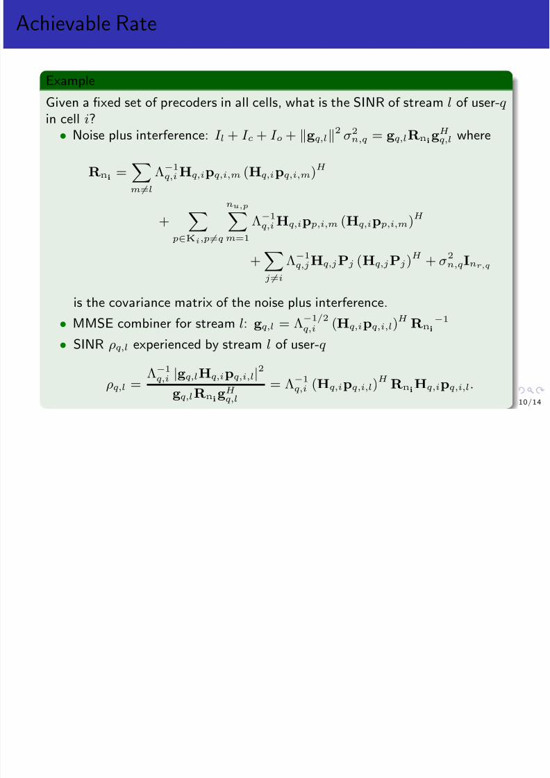
8/12/2019 Wireless Communications Lectures
http://slidepdf.com/reader/full/wireless-communications-lectures 244/271
+j=i
Λ−1q,jHq,jPj (Hq,jPj )H + σ
2
n,qInr,q
is the covariance matrix of the noise plus interference.
• MMSE combiner for stream l: gq,l = Λ−1/2q,i (Hq,ipq,i,l)H
Rni
−1
• SINR ρq,l experienced by stream l of user-q
ρq,l =Λ−1
q,i |gq,lHq,ipq,i,l|2
gq,lRnigH
q,l
= Λ−1q,i (Hq,ipq,i,l)H
RniHq,ipq,i,l.
10/14
Classical Inter-Cell Interference Mitigation
• Divide-and-conquer approach:– fragmenting the network area into small zones independently controlled from each other– making progressively use of advanced error correction coding, link adaptation, frequency
selective scheduling and lately single-user and multi-user MIMO in each of those zones.

8/12/2019 Wireless Communications Lectures
http://slidepdf.com/reader/full/wireless-communications-lectures 245/271
Figure: Frequency Reuse Partitioning. Figure: Static Fractional Frequency Reuse.
11/14
Towards Multi-Cell MIMO: Coordination and Cooperation
• Jointly allocate resources across the whole network (and not for each cellindependently) and use the antennas of multiple cells to improve the received signalquality at the mobile terminal and to reduce the co-channel interferences.
• Two categories:– Coordination: No data sharing (user data is available at a single transmsitter) - CSI
sharing– Cooperation: Data sharing (user data is available at multiple transmsitters) - CSI
sharing

8/12/2019 Wireless Communications Lectures
http://slidepdf.com/reader/full/wireless-communications-lectures 246/271
12/14
Coordination
• Modelled by an Interference Channel in Information Theory– Optimal strategies known only for a two-user case in very weak and very strong
interference regimes

8/12/2019 Wireless Communications Lectures
http://slidepdf.com/reader/full/wireless-communications-lectures 247/271
Figure: Illustration of a two-user SISO ICin a two-cell cluster.
Figure: Achievable multiplexing gain per
user of the two-user Gaussian SISO IC(α = INR/SNR).
• In practice: coordinated scheduling (CS), beamforming (CB) and power control (PC)13/14
Cooperation
• Modelled by a Broadcast Channel (for Downlink) and Multiple Access Channel (forUplink) in Information Theory
• Reuse the analysis and tools designed for MU-MIMO• One major difference for the BC: No sum power constraint anymore but per BS
power constraint
• Sometimes called Joint Transmission or Network MIMO

8/12/2019 Wireless Communications Lectures
http://slidepdf.com/reader/full/wireless-communications-lectures 248/271
14/14
Lecture 18: MIMO in LTE/LTE-A
Bruno Clerckx
EE4-65/EE9-SO27 Wireless CommunicationsDepartment of Electrical and Electronic Engineeing
Imperial College London

8/12/2019 Wireless Communications Lectures
http://slidepdf.com/reader/full/wireless-communications-lectures 249/271
Imperial College London
January 2014
1 / 2 0
Contents
1 System Requirements
2 Frame Structure
3 Key Downlink TechnologiesReference SignalsMIMO Feedback
4 Key Uplink Technologies
8/12/2019 Wireless Communications Lectures
http://slidepdf.com/reader/full/wireless-communications-lectures 250/271
4 Key Uplink Technologies
5 Downlink Performance EvaluationsSU-MIMOMU-MIMOMulti-cell MIMO
2 / 2 0
Reference Book
• Bruno Clerckx and Claude Oestges, “MIMO Wireless Networks: Channels,Techniques and Standards for Multi-Antenna, Multi-User and Multi-Cell Systems,”Academic Press (Elsevier), Oxford, UK, Jan 2013.
– Chapter 14 15

8/12/2019 Wireless Communications Lectures
http://slidepdf.com/reader/full/wireless-communications-lectures 251/271
– Chapter 14,15
3 / 2 0
System Requirements
• peak rate– highest theoretical throughput achievable with SU-MIMO spatial multiplexing but are
typically not achieved in practical deployments.– e.g. 8x8 Spatial multiplexing with 8 streams transmission
• cell average spectral efficiency
– average spectral efficiency of a cell (with K users).– much more representative of throughput encountered in practice
• cell edge user spectral efficiency– spectral efficiency achieved by at least 95% of the users in the network.– much more representative of throughput encountered in practice

8/12/2019 Wireless Communications Lectures
http://slidepdf.com/reader/full/wireless-communications-lectures 252/271
4 / 2 0
Frame Structure
• Multiplexing/Access– DL: OFDM– UL: DFT-Spread OFDM (SC-FDM)
• Frame structure– OFDMA/SC-FDMA create a
time-frequency grid composed of time-frequency resources
– A resource block (RB) is formed by 12consecutive REs in the frequencydomain for a duration of 7 OFDMsymbols in the time domain.
– A subframe is formed of 14
consecutive OFDM/SC-FDM symbolsS h d li d d t t i i i

8/12/2019 Wireless Communications Lectures
http://slidepdf.com/reader/full/wireless-communications-lectures 253/271
consecutive OFDM/SC FDM symbols.– Scheduling and data transmission isperformed at the RB-level with theminimum scheduling unit consisting of two RBs within one subframe.
– First 3 symbols used to carry controlinformation.
5 / 2 0
Key Downlink Technologies
• Antenna configurations: 2, 4 or 8 transmit antennas and a minimum of 2 receiveantennas
• LTE Rel. 8 (finalized in Dec 2008):– Up to 4x4 (up to 4 stream transmission)– Transmit diversity (to protect against fading) using Orthogonal Space-Frequency Block
Coding (O-SFBC) for 2Tx, non-orthogonal SFBC for 4TX
– Open-loop (for high speed) Spatial Multiplexing with rank adaptation based onpredefined precoders
– Closed-loop (for low speed) Spatial Multiplexing based on codebook precoding– Stone-age MU-MIMO based on common reference signals (CRS)
• LTE Rel. 9 (finalized in Dec 2009):– Up to 4x4 (up to 4 stream transmission)– Introduction of demodulation reference signals (DM-RS)– Enhancement of MU-MIMO to support ZFBF-like precoding

8/12/2019 Wireless Communications Lectures
http://slidepdf.com/reader/full/wireless-communications-lectures 254/271
Enhancement of MU MIMO to support ZFBF like precoding
• LTE-A Rel. 10 (finalized mid 2011):– Up to 8x8 (up to 8 stream transmission)– New channel measurement reference signals (CSI-RS)– New feedback mechanisms for 8Tx (similar to adaptive codebook)
• LTE-A Rel. 11 (finalized in Dec 2012):
– Coordinated Multi-Point Transmission/Reception (CoMP) for Homogeneous (Macro)and heterogeneous (pico, DAS) networks
• LTE-A Rel. 12 on-going
6 / 2 0
Reference Signals
Dedicated RS (DRS) Common RS (CRS)
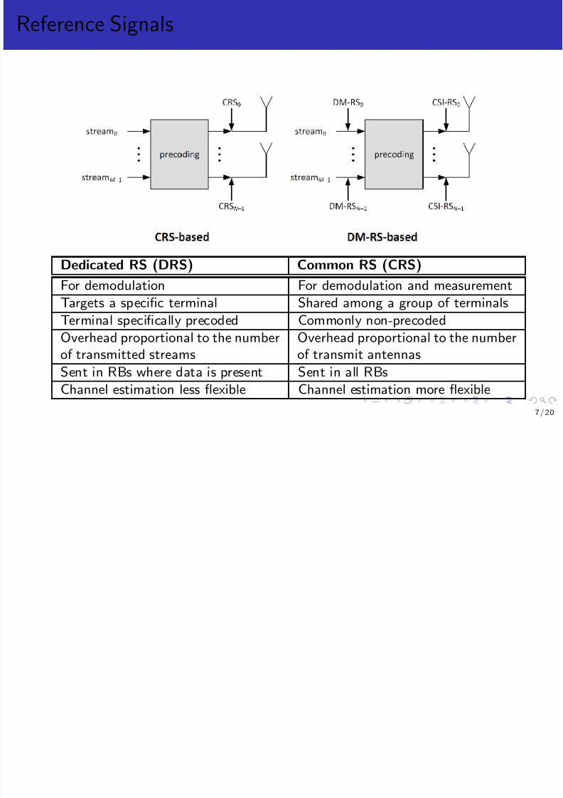
8/12/2019 Wireless Communications Lectures
http://slidepdf.com/reader/full/wireless-communications-lectures 255/271
Dedicated RS (DRS) Common RS (CRS)
For demodulation For demodulation and measurement
Targets a specific terminal Shared among a group of terminals
Terminal specifically precoded Commonly non-precoded
Overhead proportional to the number
of transmitted streams
Overhead proportional to the number
of transmit antennasSent in RBs where data is present Sent in all RBs
Channel estimation less flexible Channel estimation more flexible
7 / 2 0
Reference Signals

8/12/2019 Wireless Communications Lectures
http://slidepdf.com/reader/full/wireless-communications-lectures 256/271
8 / 2 0
MIMO Feedback
• Three main feedback information:– Rank Indicator (RI): the preferred number of streams (denoted as layers in LTE) a user
would like to receive– Precoding Matrix Indicator (PMI): the preferred precoder in the codebook– Channel Quality Indicator (CQI): the rate achievable with each stream (used to
perform link adaptation)
• Open-Loop relies only on RI and CQI– High mobility or limited CSI feedback prevent the use of PMI
• Closed-Loop (Spatial Multiplexing and MU-MIMO) rely on RI, CQI and PMI– If Spatial Multiplexing, the actual precoder is the same as the one selected by the user
(PMI)– If MU-MIMO based on CRS, the actual precoder is the same as the one selected by the
user (PMI)– If MU-MIMO based on DM-RS, the actual precoder (e.g. ZFBF) is computed based on

8/12/2019 Wireless Communications Lectures
http://slidepdf.com/reader/full/wireless-communications-lectures 257/271
p ( g ) pthe one selected by the user (PMI).
9 / 2 0
Key Uplink Technologies
• Antenna configurations: 1, 2 or 4 transmit antennas in the uplink with a minimum of 2 receive antennas
• LTE Rel. 8 (finalized in Dec 2008):– single antenna transmission and transmit antenna selection– MU-MIMO
• LTE-A Rel. 10 (finalized mid 2011):– Spatial Multiplexing with codebook– Transmit diversity (for control channels)
• LTE-A Rel. 11 (finalized in Dec 2012):– Coordinated Multi-Point Transmission/Reception (CoMP)
• LTE-A Rel. 12 on-going

8/12/2019 Wireless Communications Lectures
http://slidepdf.com/reader/full/wireless-communications-lectures 258/271
10/20
Antenna Deployments

8/12/2019 Wireless Communications Lectures
http://slidepdf.com/reader/full/wireless-communications-lectures 259/271
11/20
Network Deployments

8/12/2019 Wireless Communications Lectures
http://slidepdf.com/reader/full/wireless-communications-lectures 260/271
12/20

8/12/2019 Wireless Communications Lectures
http://slidepdf.com/reader/full/wireless-communications-lectures 261/271
SU-MIMO
Antenna deployment (with 6RB)
8x2 (0.5,15) 4x2 (0.5,15) 4x2 (4,15)2
2.25
2.5
2.75
3
c e l l a v e r a g e t h r o u g h p u t
[ b i t s / s / H z / c e l l ] ULA
DP
8x2 (0.5,15) 4x2 (0.5,15) 4x2 (4,15)0
0.05
0.1
0.15
c e l l e d g e t h r o u g h p u t
[ b i t s / s / H z / u s e r ] ULA
DP
Observations:
Antenna configuration (for ULA)
1 RB 3 RB 6 RB 50 RB1.5
2
2.5
3
3.5
4
c e l l a v e r a g e t h r o u g h p u t
[ b i t s / s / H z / c e l l ]
1 RB 3 RB 6 RB 50 RB0
0.05
0.1
0.15
0.2
c e l l e d g e t h r o u g h p u t
[ b i t s / s / H z / u s e r ] 2x2 (4,15)
4x2 (4,15)4x4 (4,15)2x2 (0.5,8)4x2 (0.5,8)4x4 (0.5,8)
2x2 (4,15)
4x2 (4,15)4x4 (4,15)2x2 (0.5,8)4x2 (0.5,8)4x4 (0.5,8)
43%
37%
50%
40%
58%
48%
65%
77%
Observations:

8/12/2019 Wireless Communications Lectures
http://slidepdf.com/reader/full/wireless-communications-lectures 262/271
• 8× 2 > 4× 2 (larger transmit array gainand SM gain).
• DP > ULA for cell average if nt large (SMgain & large array gain on each pol).
• ULA>DP for cell edge (large array gaindue to spatial correlation).
• Large AS < small AS (large array gain >
large SM gain).
• 4× 2 ≥ 2× 2, 4× 4 >> 4× 2 (symmetricconf. better).
• gain of large nr higher for less correlatedscenarios and large subband size.
14/20
SU-MIMO
Statistics of the transmission rank
1 2 3 40
0.5
1
p r o b a b i l i t y
3 RB, ULA, 4λ, 15°AS
1 2 3 40
0.5
1
p r o b a
b i l i t y
3 RB, ULA, 0.5λ, 8°AS
1 2 3 40
0.5
1
number of transmitted streams
p r o b a b i l i t y
6 RB, 0.5λ, 15°AS
4x2 ULA
8x2 ULA8x2 DP
2x2
4x24x4
2x2
4x24x4
Observations:
Channel estimation errors (ULA,3RB)
2x2 4x2 4x4 2x2 4x2 4x42
2.5
3
3.5
4
c e l l a v e r a g e t h r o u g h p u t
[ b i t s / s / H z / c e l l ]
2x2 4x2 4x4 2x2 4x2 4x40.05
0.1
0.15
0.2
c e l l e d g e t h r o u g h p u t
[ b i t s / s / H z / u s e r ]
ideal CSI−RS, ideal DM−RS
non−ideal CSI−RS, ideal DM−RSnon−ideal CSI−RS, non−ideal DM−RS
(4,15) (0.5,8)7%
7%4%
6%
4%
6%
Observations:

8/12/2019 Wireless Communications Lectures
http://slidepdf.com/reader/full/wireless-communications-lectures 263/271
• higher ranks as nt, nr, spacing and ASincrease.
• higher ranks for DP than ULA.
• rank-1 transmission most encountered.
• symmetric antenna set-up: full ranktransmission negligible.
• loss of 6 to 7% in the cell average and celledge throughputs.
15/20
SU-MIMO
Feedback subband size
2x2 4x2 4x4 2x2 4x2 4x41.5
2
2.5
3
3.5
4
c e l l a v e r a g e t h r o u g h p u t
[ b i t s / s / H z / c e l l ]
2x2 4x2 4x4 2x2 4x2 4x40
0.05
0.1
0.15
0.2
c e l l e d g e t h r o u g h p u t
[ b i t s / s / H z / u s e r ]
1 RB3 RB6 RB50 RB
(0.5,8)(4,15)
39%
14%31%
13%
42%
16%
30%11%
Observations:
Quantized and unquantized PMI
4x2 ULA (0.5,15) 4x2 DP (0.5,15) 8x2 DP (0.5,15)
2
2.5
3
3.5
c e l l a v e r a g e t h r o u g h p u t
[ b i t s / s / H z / c e l l ] quantized PMI
unquantized PMI
4x2 ULA (0.5,15) 4x2 DP (0.5,15) 8x2 DP (0.5,15)0.06
0.08
0.1
0.12
c e l l e d g e t h r o u g h p u t
[ b i t s / s / H z / u s e r ]
6% 6.5%
11.5%
4%
13.5%
7%
Observations:

8/12/2019 Wireless Communications Lectures
http://slidepdf.com/reader/full/wireless-communications-lectures 264/271
Observations:
• as the subband size increases, theperformance decreases (due to channelfrequency selectivity)
• less pronounced in spatially correlated
environment (0.5, 8).
Observations:
• loss incurred by codebook quantizationlarger in DP compared to ULA deploymentsand in 8× 2 compared to 4× 2.
16/20
MU-MIMO
Antenna deployment
8x2 (0.5,15) 4x2 (0.5,15) 4x2 (4,15)2
2.5
3
3.5
4
c e l l a v e r a g e t h r o u g h p u t
[ b i t s / s / H z / c e l l ] ULA
DP
8x2 (0.5,15) 4x2 (0.5,15) 4x2 (4,15)0
0.05
0.1
0.15
c e l l e d g e t h r o u g h p u t
[ b i t s / s / H z / u s e r ] ULA
DP
Observations:
Antenna configuration
DP ULA2
3
4
5
6
c e l l a v e r a g e t h r o u g h p u t
[ b i t s / s / H z / c e l l ] 4x2 (0.5,15)
8x2 (0.5,15)
8x4 (0.5,15)
DP ULA0.05
0.1
0.15
0.2
c e l l e d g e t h r o u g h p u t
[ b i t s / s / H z / u s e r ]
Observations:

8/12/2019 Wireless Communications Lectures
http://slidepdf.com/reader/full/wireless-communications-lectures 265/271
• ULA > DP for cell average for any nt
• ULA > DP at the cell edge
• 0.5λ > 4λ
• 8x4 provides significant gain over 8x2
– 8Tx ZFBF is far from nulling out MUinterference
– more pronounced in DP
17/20
MU-MIMO
MU-MIMO dimensioning without overhead
4x2, q. CDI 4x2, unq. CDI 8x2, q. CDI 8x2, unq. CDI2
2.5
3
3.5
4
4.5
c e l l a v e r a g e t h r o u g h p u t
[ b i t s / s / H z / c e l l ]
4x2, q. CDI 4x2, unq. CDI 8x2, q. CDI 8x2, unq. CDI0.05
0.075
0.1
0.125
0.15
c e l l e d g e t h r o u g h p u t
[ b i t s / s / H z / u s e r ] max−2 streams
max−4 streams
max−2 streams
max−4 streams
14%
14%
9%
Observations:
CSI measurement and feedback
1
1.5
2
2.5
3
3.5
c e l l a v e r a g e t h r o u g h p u t
[ b i t s / s / H z / c e l l ]
u n q . C D I / C Q I
i d . C S I / D M − R S
u n q . C D I / C Q I
n o n − i d . C S I
i d . D M − R S
u n q . C D I / C Q I
n o n − i d . C S I / D M − R S
u n q . C D I / q . C Q I
n o n − i d . C S I / D M − R S
q . C D I / C Q I
n o n − i d . C S I / D M − R S
0.075
0.1
0.125
c e l l e d g e t h r o u g h p u t
[ b i t s / s / H z / u s e r ]
42%23%16%
30%
Observations:

8/12/2019 Wireless Communications Lectures
http://slidepdf.com/reader/full/wireless-communications-lectures 266/271
• 4× 2: 4 streams > 2 streams with accuratefeedback, 2 streams > 4 streams withquantized feedback
• 8× 2: 4 streams > 2 streams if accurateand quantized feedback
• ranking of losses in increasing order of severity: CSI-RS < q. CQI < DM-RS <<
q. CDI (assuming 6RB subband size andfeedback delay)
18/20
Multi-cell MIMO
Which users benefit from cooperation?
−500 −400 −300 −200 −100 0 100 200 300 400 500−600
−400
−200
0
200
400
600
12
45
6
78
9
1011
12
1314
15
1617
18
1920
21
12
45
6
78
9
1011
12
1314
15
1617
18
1920
21
1
2
45
6
78
9
1011
12
1314
15
1617
18
1920
21
x [m]
y [ m
]
3
−500 −400 −300 −200 −100 0 100 200 300 400 500−600
−400
−200
0
200
400
600
12
3
45
6
78
9
1011
12
1314
15
1617
18
1920
21
12
3
45
6
78
9
1011
12
1314
15
1617
18
1920
21
12
3
45
6
78
9
1011
12
1314
15
1617
18
1920
21
x [m]
y [ m
]
600
78
78
78

8/12/2019 Wireless Communications Lectures
http://slidepdf.com/reader/full/wireless-communications-lectures 267/271
−500 −400 −300 −200 −100 0 100 200 300 400 500−600
−400
−200
0
200
400
12
45
6
9
1011
12
1314
15
1617
18
1920
21
12
45
6
9
1011
12
1314
15
1617
18
1920
21
12
3
45
6
9
1011
12
1314
15
1617
18
1920
21
x [m]
y [ m ]
19/20
Beyond LTE-A: Massive Multi-Cell and MassiveMulti-Antenna Networks

8/12/2019 Wireless Communications Lectures
http://slidepdf.com/reader/full/wireless-communications-lectures 268/271
20/20
Lecture 19&20: Revision and further info about
exam
Bruno Clerckx
EE4-65/EE9-SO27 Wireless Communications
Department of Electrical and Electronic EngineeingImperial College London

8/12/2019 Wireless Communications Lectures
http://slidepdf.com/reader/full/wireless-communications-lectures 269/271
January 2014
1 / 3
Exam
• Exam (written, 3 hours, closed book): 70%; Project (using Matlab): 30%• You should understand all what has been covered in the lectures. The book is there
to help and clarify the content of the lecture notes. Exam is based on theunderstanding you should acquire from the lectures/lecture notes.
• 3 questions, each question made of sub-questions.• Do not only give an answer. Explain your reasoning as much as possible!• First question addresses fundamental principles, e.g.
– Given a channel matrix, write the expression of basic MIMO receive combiner, e.g.matched filter, ZF, MMSE. Understand the difference between them.
– Given BER vs SNR or capacity vs SNR, derive the diversity gain or multiplexing gain.Relate the achievable diversity gain/multiplexing gain to transmission/receptionstrategies and antenna configurations.
Similar problems in Problem sheet 1 - Lecture 1&2 question 3 (Matlab), Problem sheet1 - Lecture 3&4 question 1 (Matlab), Problem sheet 3 - Lecture 7,8&9 question 2(Matlab)

8/12/2019 Wireless Communications Lectures
http://slidepdf.com/reader/full/wireless-communications-lectures 270/271
(Matlab)– Explanations of basic theories discussed in the course, e.g. diversity-multiplexing
tradeoff, capacity region, ....See for example Problem sheet 5 - Lecture 13&14 questions 1,2,3 (On a sheet of paper)
– Predict the performance (e.g. diversity gain) of a space-time code.See for example Problem sheet 3 - Lecture 7,8&9 question 3 (On a sheet of paper)
2 / 3
Exam
• Second question requires more thinking. Statements are made and you are asked toexplain the validity of each statement by giving a proof, example(s) and/orcounter-example(s). Statements can cover any topic in the course.See for example Problem sheet 1 - Lecture 3&4 question 4 (On a sheet of paper),Problem sheet 2 - Lecture 5&6 question 2,4,5 (On a sheet of paper).
• Third question consists in applying techniques and transmission/reception strategiesto some particular scenarios and assess the performance, e.g. write system model,design receive combiners, precoders, power allocation strategies, compute (average)error probability or sum-rate, ...See for example Problem sheet 1 - Lecture 1&2 questions 2,4,5,6 (On a sheet of paper), Problem sheet 3 - Lecture 10 question 2,3 (On a sheet of paper), Problem
sheet 4 - Lecture 11 question 1,2,3 (On a sheet of paper), the system model andderivation of the expression of the rate achievable with any receiver listed in thej LTE

8/12/2019 Wireless Communications Lectures
http://slidepdf.com/reader/full/wireless-communications-lectures 271/271
project on LTE.• You should be able to perform basic matrix analysis and derivations (similar to those
involved in the lectures). Complicated expressions of MGF (E.g. Theorem D.1 inappendix D) or matrix properties (as in Appendix A) are not to be remembered by
heart. They will be provided if necessary.
3 / 3