1

Wind Turbine System Identification Final Report MAE 566 Sean Semper and Sumit Tripathi 5/7/2009

Table of Contents Introduction/Background ........................................................................................................................................ 3

Goals ................................................................................................................................................................... 3 Wind Turbine System Model .................................................................................................................................. 4

Wind Speed and Direction: ................................................................................................................................. 4 Rotor: .................................................................................................................................................................. 4 Gear Box: ............................................................................................................................................................ 4 Electrical Generator: ........................................................................................................................................... 4 Physical Models: ................................................................................................................................................. 5 Wind Turbine Types ........................................................................................................................................... 5

Actual Data ............................................................................................................................................................. 6 Input – Output Data ............................................................................................................................................ 6 Sensors: (WMU Specific) ................................................................................................................................... 7 Tachometers: & Power Meter: ............................................................................................................................ 7

System Identification (SysID) Methods.................................................................................................................. 8 Time Domain Methods ....................................................................................................................................... 8

Linear Difference Model (1): Autoregressive Exogenous (ARX) .................................................................. 8

Model .............................................................................................................................................................. 8

Linear Difference Model (2): Autoregressive Moving Average .................................................................... 8

Exogenous Model (ARMAX) ......................................................................................................................... 8

Linear Programming ....................................................................................................................................... 8

System Realization and Frequency Response Functions (FRF) ....................................................................... 10 Eigensystem Realization Algorithm (ERA).................................................................................................. 10

DFT and Coherence Function ....................................................................................................................... 10

Kalman Filter for State Estimation ................................................................................................................... 11 Results (SkyStream3.7) .......................................................................................................................................... 12

ERA................................................................................................................................................................... 12 Hankel Matrix System Order Reduction ....................................................................................................... 12

DFT and Coherence Function ....................................................................................................................... 13

ARX and ARMAX ........................................................................................................................................... 14 Power Curve Investigation ............................................................................................................................ 14

Prediction of y(k) and Variable Wind Speed Prediction (High and Low) .................................................... 15

Kalman Filter .................................................................................................................................................... 16 State Estimation of Identified Discrete-Time Model (Wind speed Input-RPM Output) .............................. 16

State Estimation of Identified Discrete-Time Model (Wind Speed Input – Power Output) ......................... 18

SysID Methods Comparisons ........................................................................................................................... 20 ARX and ARMAX ....................................................................................................................................... 20

ARX and Linear Programming ..................................................................................................................... 21

Conclusions ........................................................................................................................................................... 22 References ............................................................................................................................................................. 22 Appendix ............................................................................................................................................................... 23

Matlab Codes .................................................................................................................................................... 23

Introduction/Background Wind Energy Systems is an area of research which is maturing rapidly due to the concern of long term global energy consumption. With advances in wind turbine technology and government decisions that are favorable to ‘green’ or renewable power, wind turbines are an increasingly viable economic alternative to conventional fossil-fuelled power generation [8]. Some of these advances are in the areas of aerodynamic blade design, new variable speed transmissions (gear boxes) and electrical generator design. Within each subcomponent nonlinear effects complicate model dynamics and the system model order (nth order > 8). Even with advance tools for system identification and control, it is impractical/ not impossible to use complex and higher order models when simpler may be available. Currently systems and dynamics research is ongoing in modeling and identification primarily for controller design, state estimation and fault detection/diagnosis. With accurate and precise system model identification, no aspect from controls to fault detection should have to employ unreasonable architectures/strategies to lower production cost and to expand the operational life of the turbine [6,7 ].

Goals The goals of this semester project are to:

o Used ERA to investigate/estimate model order (degree) and State Space Model o Compare Power Curves of identified model and Manufactures specifications o Estimated/predicted output power based on wind speed input (ARX and ARMAX) o Identify a SkyStream3.7 Wind turbine o Used Optimal Filtering (Kalman Filter) for improved state prediction

RPM and kW

Wind Turbine System Model Individual wind turbine components by themselves are quite complex far more the whole system itself. A total “system model” consists of the following: Wind, Rotor, Gear Box, and Electrical Generator, all with various parameters and dynamics which describe the system, see Figure 1. Wind Speed and Direction: Usually overlooked by consumers and must be properly calculated and if simulated one must use special distributions such as Weibull [3]. Rotor: Aerodynamic Research has pushed this portion to feasible cost effective designs. This captures the Energy from the wind, usually there is more energy in the wind than actually outputted in electrical energy however there is a physical limit called the Betz Limit which limits the actual power captured. [1]http://ww.alliantenergy.com/wcm//groups/wcm_internet/documents/image/015077-2.jpg

[2] Product Ad. [3] http:// 2.bp.blogspot.com/_WyIc2oXjvmc/S AczhuyGIgI/AAAAAAAAAfo/-leD5JgDlZU/s400/Vestas%2Brotor%2Blifting .jpg Gear Box: Transmission. Device or mechanism for transmitting the power of the rotor to that of the load, most commonly used for converting the low speed of the main shaft to the high speed required by a generator [3]. Simple Fix speed to Variable Speed gear selections are the two main types with the latter optimized for higher energy yields, lower component stress, and fewer grid connection power peaks. A generalized schematic of a typical wind turbine gearbox is shown in Figure 4. Electrical Generator: Creates the electrical power from the torque of rotor, see Figure 5 Advances in circuits/electronics and materials enhances consistent power output. Many wind turbines produced use Asynchronous AC generators (alternators) for their simple construction, starting speeds and torque characteristics [5].

Figure 1

Figure 2 Figure 3

[4] http:// www.nrel.gov/docs/fy07osti/41548.pdf [5] http:// www.windmission.dk/workshop/BonusTurbine.pdf

Physical Models: Black – Nothing is assumed Grey – Some dynamics and model orders are understood

White – Complete with all equations and parameters must be identified or matched closely

For our wind turbine model we assume all “black boxes” for relationships set forth for identification. Basic properties are provided through the manufactures produced brochures, but detailed parameters such as inertia are not available for use.

Wind Turbine Types There are three general types of wind turbines that range in size and power output from approximately 1 meter to over 120 meters and les than a 1kW to over 3 MW. Most if not all types have specific goals to meet from the personal home owner to backing up the power grids of towns and cities.

Household Medium LargeRotor Diameter (m) 1 to 20 20 to 50 50 and above

Hieght (m) 1 to 45 45 to 100 100 and abovePower Output (kW) 0.1 to 20 100 to 500 500 and above

Table 1

We will perform system identification of two types, specifically the Vestas V82-1.65 MW and SkyStream3.7 models. Where the Vestas is a Large Type and the SkyStream is a Household Type, despite the various types these two turbines currently have accessible data logs.

Figure 4

Figure 5

Figure 6

Actual Data

Input – Output Data Wind Turbine was collected from two free sources on the internet pages, Carlton College located in Northfield (“Green Carlton”), Minnesota and Western Michigan University located in Kalamazoo Michigan (“WMU Alternative and Renewable Energy Research”). Both institutions logged data from electronic sensors and meters, but WMU provided more in depth data formatting and information for downloading. However the latter datasets will be used to for system identification. Carlton College’s charted datasets extends to 2004 to 2009 for monthly Energy Output (kWh) totals, while the monthly daily output (kWh) totals range from October 2008 to April 2009. Within daily totals the average kW and wind speeds are recorded, providing a needed input-output relationship for identification.

At WMU the datasets extends from July 3, 2008 to March 31, 2009 which is viewable or downloadable in a .csv format. Parameters available from the dataset are RPM, Output (W) Power, Regulated Power (W), Wind Speed Estimate (m/s) and Watt Hours. At their website they note, “Data from the turbine is logged at nominal 1 second intervals and the tabular view of data is limited to 1000 records…” Upon inspection of the “second interval” data we noticed the sample time per minute varied from 1 sample per minute to 46 samples per minute, which were indications of future issues with the identification Methods. However minute, hour and day averaged data was available for selection and use. For our identification we used the minute data from a minimum of hours to a whole month since the sample time was shorter.

Figure 7

Sensors: (WMU Specific) Anemometer: We assumed a high performance wind sensor is used for the dataset source. From WMU’s

webcam we visual noted a similar anemometer to SUTRON WINS SENSOR PROP VANE 5600-0200 and used it specifications (σ ≈ 1% of reading) for estimation purposes.

Figure 8

Tachometers: & Power Meter: RPM and kW readings sensor statistics are not given but collected through a wireless link and computer software for turbine performance monitoring.

System Identification (SysID) Methods

Time Domain Methods

Linear Difference Model (1): Autoregressive Exogenous (ARX)

Model ARX model:

The parameters are solved using Least Square algorithm. Above equation can be written in matrix form.

, ,

Linear Difference Model (2): Autoregressive Moving Average

Exogenous Model (ARMAX) Further refinement in predicted values is possible with incorporation of error modeling. We followed ARMAX algorithm to predict based on error vector of predicted output from ARX and actual output. By describing error as moving average of white noise we have,

For m predictions, formulating MATRIX similarly, we can write

, ,

Linear Programming We can approach our problem with linear programming concepts. Although, the actual problem might be of non-linear form, it is possible to simplify a nonlinear optimization problem by linearization and then solving it using Linear programming techniques. We can take next predicted output as a function of previous outputs and inputs as we did in ARX. However, here we will use MALLAB ‘linprog’ command to minimize the error of predication by posing it as optimization problem.

Considering the discrete ARX series

The objective is to minimize error Where is the measured output signal. The problem can be posed as linear programming problem as follows

For all K. We have used ‘linprog’ command to implement linear programming. X=LINPROG(f,A,b) attempts to solve the linear programming problem: min f'*x subject to: A*x <= b x For our problem f become a row vector with all the terms as zero except last term that is the term for our cost function ‘t’. A is the matrix of time shift values of y(k) and u(k). From equation (1)

And

Combining equation (2) and (3) for multiple record data, we get our A and b matrix for linprog.

X is a vector containing coefficients of and coefficients of

System Realization and Frequency Response Functions (FRF)

Eigensystem Realization Algorithm (ERA) Determining Order of the model: We approached with Hankel order reduction technique. We begin with finding out Markov parameters of the system with Frequency Response Function

Where, are the DFT of output and input vectors. is transpose of Markov parameters The Hankel matrix can be formed with Markov parameters as follows

Now we examine singular values of block Hankel Matrix H0. Only relatively large values are due to true modes of the system. The relatively small singular values may be ignored as they contain more noise information than system information. With the information on order of the system we can now proceed for power predication. To find minimum order realization [ , we use H(0) and shifted block Hankel matrix H(1)

Where n = Identified Order of the System from Singular Values of ∑

Note (1): ERA/DC Even at this stage we want to get rid of any noise in Markov parameters to have better examination of singular values. Data correlation technique is again used. If noise in the Markov Parameters are not correlated, the correlation matrix H0*H0’ will contain less noise than the Hankel matrix H0. Hence, we examine singular values of H0*H0’ in order to observe any noise reduction of the states. Note (2): Modal Amplitude Coherence (MAC) This method is a check for the identified State-Space Model to see if it will reproduce the pulse response data. If the value is 1 for the MAC then the identified model can be used for the system, which is just a different state transformation.

DFT and Coherence Function Checking input-output noise levels with coherence function: In order to qualify the computed frequency response function, we use coherence function. The coherence function between input and the output is defined as

is average cross-spectral density between the input and the output. is the complex conjugate of . is the autocorrelation functions between the outputs. The coherence function value always lies between 0 and 1 1>= >=0 The coherence is unity with negligible noise. On the other hand if noise is not negligible but is uncorrelated wit the input signal, the coherence function is zero. It is worth noting that any leakage problem in FRF due to improper periodicity of the input/ output data will contribute to poor coherence. The leakage problem can be solved by windowing the input/output data. We used Hamming window for our analysis.

Kalman Filter for State Estimation With an identified system model the Kalman Filter is used to enhance system state prediction. Since it is an Optimal State Estimator which handles noise measurement and inaccurate system models we will look for any improvements over ARX and ARMAX output predictions. The overall flow of the algorithm is as follows:

Results (SkyStream3.7)

ERA

Hankel Matrix System Order Reduction

Figure 9

Decomposition of H(0) reveals four dominating σi in Figure 9. From 5th to 20th singular values (σi ≈ σ5 … σ20) are relatively small and are omitted. Hence the order of the system (wind speed input and power output) is taken as n = 4. Further results in the Kalman Filter Results Section will use ERA to discover intermediate relationships within the wind turbine.

0 2 4 6 8 10 12 14 16 18 200

0.1

0.2

0.3

0.4

0.5

0.6

0.7

0.8

0.9

1Normalized Singular Values σ(i) of Hankel Matrix with DC

Nor

mal

ized

σ(i)

DFT and Coherence Function

Figure 10

Figure 11

It is clear from Figures 10 & 11 that windowing helps to improve coherence by reducing the leakage problem. This problem might be there due to the lack of periodicity in the input and output signals.

0 0.05 0.1 0.15 0.2 0.25 0.3 0.35 0.4 0.45 0.50.4

0.5

0.6

0.7

0.8

0.9

1Coherence between "Wind Speed" and "Watts"-Raw Data

Frequency

0 0.05 0.1 0.15 0.2 0.25 0.3 0.35 0.4 0.45 0.50.4

0.5

0.6

0.7

0.8

0.9

1

Coherence between input "Wind Speed" and output "Watts"with Hamming Window

ARX and ARMAX

Power Curve Investigation

Figure 12

From Figure 12 the plot of Power Vs. Wind speed, it is clear we have much less power contribution for power generation from wind speed less than 3 m/s. This gives motivation to solve for different parameter sets for different wind speed range. [parsol_H]=ARX_model(mb,na,u_in,y_out) %Parameters solved by wind speed 3 to 20 parsol_H = 1.0e+002 * 0.00314431982496 0.00197149892957 0.00419248381483 1.18846704373996 -0.32658292076718 -0.33721715858577 -0.49947948696246 [parsol_L]=ARX_model(mb,na,u_in,y_out) )%Parameters solved by wind speed 0 to 3 parsol_L = 0.27436706116393 0.21191000048309 0.14685638790042 7.26211367238954 -0.37655912755919 -1.51050438089302 -2.11611181449937 “u_in” and “y_out” are the preprocessed input (wind speed) and output (power) vectors.

2 4 6 8 10 12 14 16 18 20 220

500

1000

1500

2000

2500

3000

X: 10Y: 1717

Wind Speed (m/s)

Pow

er O

utpu

t (kW

)

Power vs. Wind Speed

X: 5Y: 270.9

X: 3Y: 29.07

Actual Power CurveMean Power Curve

Prediction of y(k) and Variable Wind Speed Prediction (High and Low) One step ahead predication by parameter solved with low speed range data gives poor prediction, as we can see from the graph below in Figure 13.

Figure 13

This implies that low speed range data is now able to capture systems’ dynamics. However, if we perform one step ahead prediction with parameters solved with high speed range data we get much better prediction, see Figure 14.

Figure 14

0 5 10 15 20 25 30 35 40 45 500

50

100

150

200

250

300

350

400

450Predicton with only Low Wind Speed data: ARX

Time(min)

Wat

tsIdentified WattsActual Watts

0 5 10 15 20 25 30 35 40 45 50-50

0

50

100

150

200

250

300

350

400

450Predicton with only High Wind Speed data: ARX

Time(min)

Wat

ts

Identified WattsActual Watts

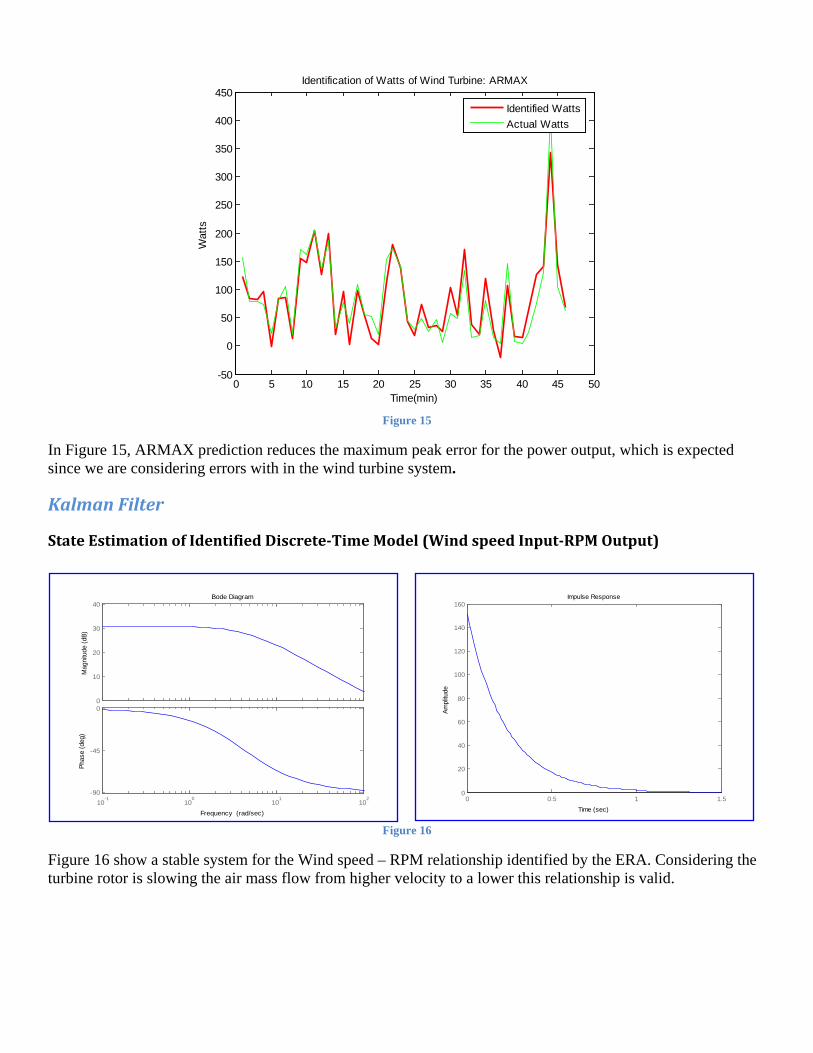
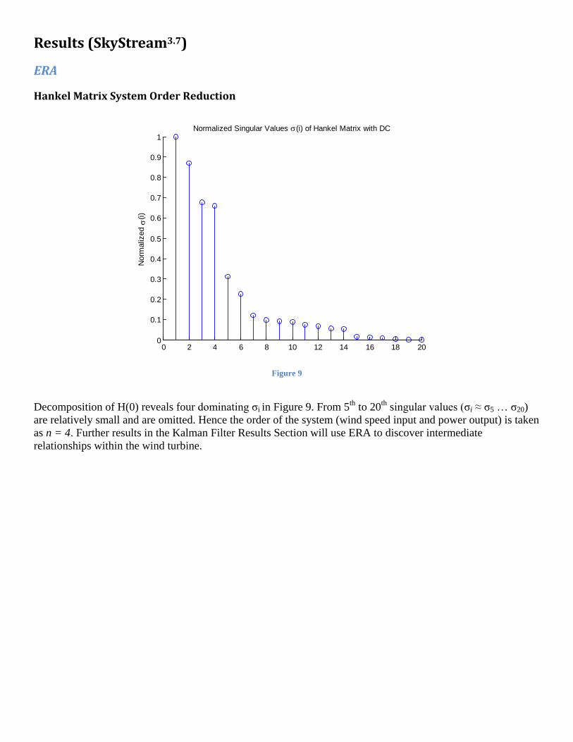
Figure 15

In Figure 15, ARMAX prediction reduces the maximum peak error for the power output, which is expected since we are considering errors with in the wind turbine system.

Kalman Filter

State Estimation of Identified Discrete-Time Model (Wind speed Input-RPM Output)

Figure 16

Figure 16 show a stable system for the Wind speed – RPM relationship identified by the ERA. Considering the turbine rotor is slowing the air mass flow from higher velocity to a lower this relationship is valid.

0 5 10 15 20 25 30 35 40 45 50-50

0

50

100

150

200

250

300

350

400

450Identification of Watts of Wind Turbine: ARMAX

Time(min)

Wat

ts

Identified WattsActual Watts

0

10

20

30

40

Mag

nitu

de (d

B)

10-1

100

101

102

-90

-45

0

Phas

e (d

eg)

Bode Diagram

Frequency (rad/sec)

0 0.5 1 1.50

20

40

60

80

100

120

140

160Impulse Response

Time (sec)

Ampl

itude

Figure 17

Simulating the realized State-Space model reveal accurate identification for the same wind speed input, see Figure above. Below we see in Figure 18, using the Kalman Filter and a separate dataset for input-output validates the estimated model, and it can be used as representation of this intermediate relationship.

Figure 18

2100 2120 2140 2160 2180 2200 2220 2240 2260 2280 2300-50

0

50

100

150

200

250

RPM

(rev

/min

)

Time (mins)

RPM vs. Time

0 0.2 0.4 0.6 0.8 1 1.2 1.4 1.6 1.8 2

x 104

-50

0

50

100

150

200

250

300

350

RP

M (r

ev/m

in)

Time (mins)

RPM vs. Time

0 500 1000 15000

50

100

150

200

250

300

350

400

time (min)

Simulation of March 1, 2009

Figure 19

In Figure 19, 1st Order System shows low error covariance prediction because of 1st dominant mode and 1% standard deviation for rpm measurement error from our sensor assumptions.

State Estimation of Identified Discrete-Time Model (Wind Speed Input – Power Output)

Figure 20

0 2000 4000 6000 8000 10000 12000 14000 16000 18000 20000-1

-0.8

-0.6

-0.4

-0.2

0

0.2

0.4

0.6

0.8

1

RPM

Est

imat

e Er

rors

Time (mins)

Errors and 3σ Bounds vs. Time

0 2000 4000 6000 8000 10000 12000-50

0

50

100

150

200

250

300

350

Pow

er O

utpu

t (W

atts

)

Time (mins)

Power Output (Watts) vs. TimeState-Space ID with March 2009 and Oct 2008 Validation

1800 1820 1840 1860 1880 1900 1920 1940 1960 1980 2000-20

0

20

40

60

80

100

120

140

160

Pow

er O

utpu

t (W

atts

)

Time (mins)

Power Output (Watts) vs. TimeState-Space ID with March 2009 and Oct 2008 Validation

Figure 21

Figure 20 & 21 plots the result for a 4th Order system identified by ERA with its estimated states for power output. Specifically in the left plot of Figure 20 we note the prediction is close but not exact due to the higher order effects of 4th Order model. Also the estimated errors for power prediction will be within +20 Watts, a reasonable error for a 2.4 kW rated system, see Figure 21.

Figure 22

Figure 22 plots the MAC for the identified State-Space Model and validates that our model can reproduce the pulse response data justifying our choice for n=4 states. Which does not mean no other models can be found for the wind turbine, just the system is satisfactory for prediction.

0 2000 4000 6000 8000 10000-80

-60

-40

-20

0

20

40

60

80

Wat

ts E

stim

ate

Erro

rs

Time (mins)

Errors and 3σ Bounds vs. Time

1 2 3 40

0.2

0.4

0.6

0.8

1

Modal Amplitude Coherence (MAC)

MAC

Val

ue

Eigenvalue Index i

Figure 23

If we check coherence function with identified states from Kalman Filter, we can see that the noise level has gone down. Since coherence is close to 1 we have negligible noise in the identified states, see Figure 23.

SysID Methods Comparisons

ARX and ARMAX

Figure 24

Clearly in Figure 24, we see ARMAX, modeling error as moving average of white noise, gives little better performance than only ARX.

0 0.05 0.1 0.15 0.2 0.25 0.3 0.35 0.4 0.450.6

0.65

0.7

0.75

0.8

0.85

0.9

0.95

1

Coherence between Identified States With Kalman Filter

ω

1 2 3 4 5 6 7 8 9 100

500

1000

1500

p

(Σx i

p ) 1

/p

Comparision of P norms between error vectorsidentified by ARX andARMAX

ARXARMAX

ARX and Linear Programming

Figure 25

We have little improvement by the method of linear programming, which is visible between 10 and 15 min in Figure 25. We can as well visualize by plot plotting p-norms of error form two methods from. Clearly, ARX error norm is always greater than Linear Programming error norm, seen in Figure 26.

Figure 26

0 5 10 15 20 25 30 35 40 45 50-50

0

50

100

150

200

250

300

350

400

450

Time minute

Wat

ts

Identification With ARX

ActualEstimate

0 5 10 15 20 25 30 35 40 45 50-50

0

50

100

150

200

250

300

350

400

450

Time(minute)

Wat

ts

Identification With Linear Programming

ActualEstimate

1 2 3 4 5 6 7 8 9 100

500

1000

1500

p

(Σx i

p ) 1

/p

Comparision of P norms between error vectorsidentified by ARX and Linear Programming

ARXLinear Programming

Conclusions We initial used ERA to investigate model order (degree) then estimated/predicted output power based on wind speed input (ARX, ARMAX and Linear Programming). Next we identified SkyStream wind turbine considering 4° - 6° models and used Optimal Filtering (Kalman Filter) for improved state prediction RPM and kW. Given a black box for the wind turbine system the overall results are provide a good description and prediction for a SkyStream Wind Turbine. If actual inertial properties were available identification for physical parameters would be then next step for the future goals.

References Books

1. Chi-Tsong. C., Linear System Theory and Design 3rd Ed, Oxford University Press, 1998. 2. Eldridge, F.R., Wind Machines, Van Nostrand Reinhold Company, New York, 1980. 3. Gipe, P., Wind Power, Chelsea Green Publishing Company, Vermont, 2004. 4. Juang, J., Applied System Identification, Prentice Hall PTR, New Jersey, 1994. 5. Rizzoni, R., Principles and Applications of Electrical Engineering 3rd Ed, Mc Graw Hill, Boston, 2000.

Journal Articles

6. Bonger, P.M.M., Experimental Validation of a Flexible Wind Turbine Model, IEEE, Proceedings of the 30th Conf. on Decision and Control, England, 1991.

7. Novak, P., Modeling and Identification of Drive-System Dynamics in a Variable-Speed Wind Turbine, IEEE, 1994.

8. Yang, W., Wind Turbine Condition Monitoring and Fault Diagnosis Using both Mechanical and Electrical Signatures, IEEE, International Conference on Advance Intelligent Mechtronics, China, July 2008.

Appendix

Matlab Codes See files “MATLAB_codes.docx” and “Codes_part2.docx”