Embed Size (px)
Citation preview

Wind Turbine Selection: A case-study for Búrfell, Iceland
by
Samuel Perkin
60 ECTS Thesis
Master of Science in Sustainable Energy Engineering
January 2014

Wind Turbine Selection: A case-study for Búrfell, Iceland
Samuel Perkin
60 ECTS Thesis submitted to the School of Science and Engineering
at Reykjavík University in partial fulfillment
of the requirements for the degree of
Master of Science in Sustainable Energy Engineering
January 2014
Supervisors:
Páll Jensson, Supervisor
Professor, Department Head, Reykjavík University, Iceland
Margrét Arnardóttir, Co-Supervisor
Project Manager (Wind Power), Landsvirkjun
Deon Garrett, Co-Supervisor
Research Scientist, Icelandic Institute for Intelligent Machines
Examiner:
Magnus Þór Jónsson, Examiner
Professor, University of Iceland, Iceland

Wind Turbine Selection: A case-study for Búrfell, Iceland
Samuel Perkin
60 ECTS Thesis submitted to the School of Science and Engineering
at Reykjavík University in partial fulfillment
of the requirements for the degree of
Master of Science in Sustainable Energy Engineering
January 2014
Student:
___________________________________________
Samuel Perkin
Supervisors:
___________________________________________
Páll Jensson
___________________________________________
Margrét Arnardóttir
___________________________________________
Deon Garrett
Examiner:
___________________________________________
Magnus Þór Jónsson

iv
ABSTRACT
The efficient selection of a wind turbine is presently limited by a developer’s knowledge of
what products are available on the market, and their ability to test and compare available
turbine designs before investing. Poor turbine selection results in a financially sub-optimal
investment. This study applies Blade Element Momentum theory, cost-scaling models and
Genetic Algorithms to produce a model that predicts the ideal turbine design for a given site.
The model was verified and tested using raw, real-world data from met masts and two
Enercon E-44 turbines installed at Búrfell, Iceland.
The model identified an optimum wind turbine design for Búrfell which decreases the
Levelized Cost of Energy by 10.4% when compared to the existing E-44 turbines. The power
curve of the optimum turbine design was then used as a search parameter in a set of real
turbines, to determine that the optimum turbine model for Búrfell is the Leitwind LTW70
2MW turbine. The use of this turbine would decrease the Levelized Cost of Energy by 8%
when compared to the existing Enercon E-44 turbines.
Future recommendations are to develop a similar model using Finite Element Analysis in lieu
of Blade Element Momentum theory, and to include optimization of the rotor shape and
material. A more up-to-date analysis of wind turbine costs is also advised.
Keywords: Wind Turbine Selection, Blade Element Momentum theory, Cost-Scaling, Genetic
Algorithms, Levelized Cost of Energy.

v
ACKNOWLEDGEMENTS
I would like to acknowledge Páll Jensson for his supervision and advice throughout the
duration of the thesis; Margrét Arnardóttir for her assistance in finding a useful problem to
solve, for providing the data that formed the basis of the thesis, and for providing insights
into the operation of the wind turbines at Búrfell; and Deon Garret for allowing use of his
Genetic Algorithm code and providing priceless advice and assistance with my C++ troubles.
I would like to thank Ágúst Valfells for his advice and initial push in the right direction, and
for Halla Logadóttir for putting me in touch with Margrét. I would also like to acknowledge
the great help and critique from Stefán Kári Sveinbjörnsson on my model, and practical
insights into the wind turbine industry.
Finally I’d like to acknowledge my family for providing the long-distance moral and
grammatical support from across the pond, and for my friends in Iceland for patiently
tolerating my wind turbine-based rants and keeping me relatively sane.

vi
CONTENTS
Abstract .................................................................................................................................... iv
Acknowledgements .................................................................................................................. v
List of figures ........................................................................................................................ viii
List of tables.............................................................................................................................. x
List of Symbols and Acronyms .............................................................................................. xi
1. Introduction ...................................................................................................................... 1
1.1. Background ................................................................................................................. 1
1.2. Research Focus ............................................................................................................ 3
1.3. Aim and Objectives ..................................................................................................... 4
1.4. Motivation ................................................................................................................... 4
1.5. Outline of thesis .......................................................................................................... 5
2. Literature review ............................................................................................................. 6
2.1. Wind Resources........................................................................................................... 6
2.2. Wind Turbines ........................................................................................................... 10
2.3. Wind Turbine Selection ............................................................................................ 12
2.4. Wind Turbine Design ................................................................................................ 16
2.5. Turbine electrical output estimation .......................................................................... 18
2.6. Wind Turbine Cost .................................................................................................... 24
2.7. Economic Analysis of Wind Power Investments ...................................................... 26
2.8. Genetic Algorithms ................................................................................................... 26
2.9. BEM, Cost-Scaling and GA based turbine optimisation models .............................. 27
3. Research methods .......................................................................................................... 31
3.1. General Model Structure ........................................................................................... 31
3.2. Size and cost constraints for wind turbine ................................................................ 33
3.3. Genetic Algorithm Population Generation ................................................................ 34
3.4. BEM Theory Loop and Rotor Blade Data ................................................................ 36

vii
3.5. Wind Data and AEP calculation................................................................................ 38
3.6. Cost Model ................................................................................................................ 38
3.7. GA fitness function and population mutation ........................................................... 41
4. Results ............................................................................................................................. 43
4.1. Wind Data Analysis .................................................................................................. 43
4.2. BEM Theory Model Verification .............................................................................. 45
4.3. Optimisation model comparison ............................................................................... 49
4.4. Sensitivity Analysis ................................................................................................... 53
5. Conclusions ..................................................................................................................... 54
5.1. Key results ................................................................................................................. 54
5.2. Model critique ........................................................................................................... 55
5.3. Future Research Recommendations .......................................................................... 56
6. References ....................................................................................................................... 57
7. Appendix ......................................................................................................................... 61
7.1. Raw Wind Data ......................................................................................................... 61
7.2. Blade profile geometry .............................................................................................. 61
7.3. Lift and drag coefficient data .................................................................................... 62
7.4. Detailed Cost Equations ............................................................................................ 63
7.5. Turbine Reference Numbers ..................................................................................... 65
7.6. C++ Code (excluding GA code implementation) ..................................................... 67

viii
LIST OF FIGURES
Figure 1: Levelized Cost of Landsvirkjun's investment options in Hydro/Geothermal power,
compared with estimated costs for infrastructure built in the US in 2016 (excluding
transmission costs) (GAM Management, 2011). ....................................................................... 2
Figure 2: Relationship between Power Coefficient and axial induction factor for an ideal rotor
.................................................................................................................................................. 11
Figure 3: Power curve of the Enercon E-44 wind turbine (Enercon, 2013a) .......................... 12
Figure 4: Annular element of wind turbine as assessed by BEM Theory (Moriarty and
Hansen, 2005) .......................................................................................................................... 19
Figure 5: Definition of relative air velocity and air flow angle (Hansen, 2008) ..................... 20
Figure 6: Breakdown of initial costs associated with a turbine constructed in 2011 (Tegen et
al., 2013) .................................................................................................................................. 25
Figure 7: Schematic diagram of the computational model developed for this study............... 31
Figure 8: Example of a possible chromosome (i.e. a unique solution in the Genetic Algorithm
model) ...................................................................................................................................... 35
Figure 9: Pseudo-code diagram for BEM Theory module, which calculates the power curve
given a set of input turbine characteristics ............................................................................... 37
Figure 10: Example of two 10 bit chromosomes undergoing uniform crossover .................... 42
Figure 11: Example of two 10 bit chromosomes undergoing bitwise mutation (black,
underlined bits are those that were altered by bitwise mutation). The mutation of Offspring A
has no effect on the mutation of Offspring B. ......................................................................... 42
Figure 12: RMSE fitted annual Weibull Distribution for wind at Búrfell, at a height of 10m 44
Figure 13: Comparison of simulated power curve (generated with BEM model) with the
Enercon E-44 power curve, and raw data from an E-44 turbine at Búrfell ............................. 46
Figure 14: Shows the same as Figure 13 above but with the raw data consolidated as an
average power curve ................................................................................................................ 46
Figure 15: Turbine comparison matrix showing the NRMSE of the simulated power curve for
each turbine, compared with the actual power curve of all other turbines (i.e. an accurate
model would have low NRMSE on the diagonal, and low NRMSE otherwise) ..................... 48
Figure 16: Impact of wind turbine generation capacity on the accuracy of the BEM code
(measured by NRMSE when comparing the modelled power curve with the manufacturer's
power curve for a specific turbine) .......................................................................................... 49
Figure 17: LCoE of optimum wind turbine verses number of evaluations performed ............ 50

ix
Figure 18: Comparison of the power curves of the optimum turbine and the most similar
turbine (Leitwind LTW70) ...................................................................................................... 51
Figure 19: Initial Cost vs AEP for all 47 turbines from Helgason, as calculated by the model,
with the optimum turbine (found by the GA model) highlighted in red .................................. 52
Figure 20: Rotor Radius vs Generator Capacity for all turbines from Helgason, with the
optimum turbine highlighted in red ......................................................................................... 52
Figure 21: A sensitivity analysis of the model, using the optimum turbine design as a baseline
design. The sensitivity of the LCoE to the three main design variables is shown, such that the
impact of changing each variable can be compared. ............................................................... 53

x
LIST OF TABLES
Table 1: Assumed values for wind turbine design variables that are not optimised in the
model........................................................................................................................................ 32
Table 2: Summary of variable constraints used to define the solution space in the model ..... 34
Table 3: Summary of bit assignment and variable precision (* Precision = 1, due to integer
rounding in the code) ............................................................................................................... 34
Table 4: Summary of monthly RMSE-fitted Weibull parameters for Búrfell ......................... 44
Table 5: Summary of monthly Weibull parameters determined by (Helgason, 2012) ............ 44
Table 6: Model input data for Enercon E-44 Turbine .............................................................. 45
Table 7: NRMSE of Enercon and Simulated power curves with the raw data from one of the
E-44 turbines at Búrfell ............................................................................................................ 47
Table 8: Results of optimisation model for a wind turbine at Búrfell based on LCoE, with
modelled results of Enercon E-44 and E-88 turbines for comparison ..................................... 50
Table 9: Comparison of the optimum turbine, as determined by the model, and the most
similar turbine in the set of 47 turbines defined in Appendix 7.5 ............................................ 51
Table 10: NREL S809 rotor blade geometry, used in BEM model (NREL, 2000) ................. 61
Table 11: NREL S809 rotor lift and drag coefficients, used in BEM model (Ramsav et al.,
1996) ........................................................................................................................................ 62
Table 12: Turbine reference list, including rotor radius and generator capacity, and NRMSE
of comparison with modelled power curve .............................................................................. 65

xi
LIST OF SYMBOLS AND ACRONYMS
AEP Annual Energy Production [GWh/year]
GA Genetic Algorithm
LCoE Levelized Cost of Energy [USD/MWh]
NPV Net Present Value [2013 US Dollars]
Wind speed at an elevation of [m/s]
Elevation measured from ground level [m]
Wind-shear coefficient [dimensionless]
Weibull shape parameter [dimensionless]
Weibull scale parameter [m/s]
Power produced at a particular wind speed [W]
Weibull distribution of wind speed , given parameters and [dimensionless]
Kinetic energy of wind [J]
Mass of a particle [kg]
Velocity of a particle [m/s]
Mass [kg]
Air density [kg/m3]
Area [m2]
Duration [s]
Axial induction factor [dimensionless]
Tangential induction factor [dimensionless]
Power coefficient [dimensionless]
Initial investment cost [2013 US Dollars]
Annual cost in year [2013 US Dollars]
Discount rate [%]
CF Capacity factor [dimensionless]
Flow angle [radians]
Angle of attack [radians]
CL Lift force coefficient [dimensionless]

xii
CD Drag force coefficient [dimensionless]
CN Normal force coefficient [dimensionless]
CT Tangential force coefficient [dimensionless]
Wind speed approaching the rotor blade [m/s]
Wind speed relative to the rotating turbine blade [m/s]
Speed of the wind turbine rotor [m/s]
Rotational speed of wind turbine rotor [radians/s]
Rotor radius at blade section [m]
Rotor pitch angle [radians]
Local pitch angle of rotor [radians]
Local blade twist angle [radians]
/ Lift/Drag coefficient adjusted for 3-dimensional rotational effects [dimensionless]
Correction factor for 3-dimensional rotational effect adjustment [dimensionless]
Chord width at rotor blade section [m]
Prandtl correction factor [dimensionless]
Secondary Prandtl correction factor [dimensionless]
Number of rotor blades on wind turbine [# of blades]
Rotor Radius [m]
Solidity factor at blade section [dimensionless]
Glauret correction factor [dimensionless]
Thrust force [N]
Point thrust force on segment on a rotor blade [N]
Moment [Nm]
Combined efficiency of gearbox and generator [dimensionless]

1
1. INTRODUCTION
The following chapter gives a general background to the thesis topic, describes the focus of
the research, and states the aims and objectives. The research motivations are also explained,
as well as a brief outline of the following chapters in the paper.
1.1. BACKGROUND
British appreciation for Iceland’s natural wind resources stretch back as far as 1871 with
William Morris’ poem ‘Iceland first seen’ (Morris, 1892) in which he describes:
The sight of this desolate strand,
and the mountain-waste voiceless as death
but for winds that may sleep not nor tire?
He acknowledges Iceland’s strong and reliable wind resources, as well as the low terrain
roughness and lack of wind-breaking obstacles. Therefore It is only fitting that a
Memorandum of Understanding for a submarine electrical transmission cable between the
United Kingdom and Iceland (DECC, 2012) was signed the same year that the first two wind
turbines in Iceland were erected (Askja Energy, 2013a). Such a cable would require
additional energy infrastructure to meet the increased demand in electricity.
The installation of the two wind turbines by Landsvirkjun at Búrfell suggests that wind power
is seen as a competitive technology and a potential means of diversifying Iceland´s renewable
energy portfolio. Currently 72.7% of Iceland’s electricity is supplied by Hydropower, 27.3%
from geothermal power plants, and 0.01% from fuel generators (Orkustofnun, 2013).
This need to grow Iceland’s energy portfolio comes, not only from the potential for a
submarine connection to the UK, but from the likelihood of new energy-intensive industries
establishing in Iceland. Approximately 79% of electrical energy is used by energy-intensive
aluminium and ferro-silicon smelters (Orkustofnun, 2013). It is likely that there will be
further growth in energy-intensive industry given Iceland’s globally competitive electricity
prices. Conversely, the average growth in non-industrial electricity demand in Iceland is
estimated to be 2.8% (Orkustofnun, 2006); equivalent to 55 MW of additional capacity
required annually.

2
Wind power in general is not competitive with the current energy infrastructure options for
investment in Iceland, shown below in Figure 1. However environmental/social concerns
may restrict future developments in geothermal and hydropower infrastructure. Development
in wind power however is supported by 81% of the population (Askja Energy, 2013b), and
has no permanent environmental impact. Wind power is also suited to operate in a portfolio
with hydropower resources, given the short-term variability of wind and the long-term
variability of water resources, which effectively mitigate one another.
Figure 1: Levelized Cost of Landsvirkjun's investment options in Hydro/Geothermal power, compared with estimated costs
for infrastructure built in the US in 2016 (excluding transmission costs) (GAM Management, 2011).
It should be noted that Figure 1 is also based on a general case-study of the USA, which does
not account for the cost of using wind resources in Iceland. Morris’ poetic assessment of
Iceland’s wind resources is supported by a more recent wind resource assessment (Nawri et
al., 2013) which states that: “The wind energy potential of Iceland is within the highest class
as defined in the European Wind Atlas”. Given these top-class wind resources and the
growing electricity demands in Iceland, the recent interest in developing wind power in
Iceland can be understood.
Regardless of when new wind turbines will be competitive or what demand they will satisfy,
Iceland is a new frontier for the wind turbine industry. It is important to verify that the
commercially available wind turbines are ideal for Icelandic applications. If the ideal turbine
does not exist, then it is equally important to determine which available turbine is most
similar to the ideal turbine.

3
1.2. RESEARCH FOCUS
The previous section discussed the growing interest in wind turbines in Iceland, specifically
the suitability of commercially available wind turbines. This thesis will focus on how
developers choose turbines from the set of available turbines, and whether the selection
process can be improved by the use of a physics-based model.
In choosing a wind turbine, the decision making progress is generally based upon the
profitability of the investment. Simply put, the turbine that produces the highest Net Present
Value (NPV) will be chosen by a rational developer. However, the decision is restricted by
the following constraints:
- Spatial (limited availability of land or wind resources);
- Capital (restrictions on the value of the initial investment);
- Capacity (limitations on the output of the turbine, due to market or technical issues);
- Availability (certain wind turbine models may not be available, or practical, to
transport to Iceland).
Spatial constraints are important to consider for wind farm design or in cases where multiple
or topographically complex sites are available for wind farm development. The impact of
spatial constraints will not be considered in this study. Instead the report will focus on a
decision involving a single turbine and a particular site, such that capital, capacity and
availability constraints can be discussed.
Based on discussions with a large energy infrastructure developer, the current approach to
turbine selection is to assume some capital and capacity constraints to create a subset of the
market-available wind turbines. The energy production of each wind turbine is then assessed
using Weibull distributions or through computational packages like WAsP (DTU National
Laboratory, 2013). A bidding process is then initiated with the manufacturers of the most
appealing turbines, in order to determine costs and to assess each turbine’s profitability. This
is in essence a brute force or trial-and-error approach to finding the optimum wind turbine.
This approach requires the assumption that the subset of commercially available turbines that
are assessed includes the ‘ideal’ turbine for the site in question. The impact of this
assumption, and how this assumption can be avoided, is the general focus of this thesis.

4
1.3. AIM AND OBJECTIVES
The overall aim of the proposed research is to create a physics-based model to design an ideal
turbine given wind-data and cost-scaling relationships for a particular site, and to compare the
results with the trial-and-error approach.
Specifically, the objectives of this research are to:
1) Identify the common goals of the wind turbine selection process
2) Evaluate critically the use of a trial-and-error approach to turbine selection
3) Develop a turbine selection model that incorporates state-of-the-art methods
4) Verify and compare the physics-based model with the trial-and-error method
5) Recommend an efficient approach to turbine selection
1.4. MOTIVATION
Identifying the common goals of the process and the metrics by which turbines are compared,
or excluded from comparison, will provide insight into how energy developers make
decisions. Clearly defined goals and metrics will provide a baseline to which turbine
selection methods can be compared. This baseline will initially be used to identify and define
the strengths and weaknesses of a trial-and-error approach to turbine selection.
From this assessment of the trial-and-error approach, a physics-based model will be justified
and developed. It is expected that a physics-based model that uses cost-scaling estimates can
effectively assess the entire set of possible wind turbine designs (including those that don’t
exist yet) on a basis of NPV or Levelized Cost of Energy (LCoE) without the need to enter a
bidding process with manufacturers. In order to verify the accuracy of the physics-based
model, it will be compared with real world data for a specific turbine at a specific site in
Iceland. The model will then be verified on the decision-making scale, by comparing the
results of the model with a recent paper by Helgason that applied the trial-and-error approach
in Iceland. From this, the motivation is to make recommendations for energy infrastructure
developers on the process of choosing a suitable wind turbine, and to provide some insights
into the characteristics of a turbine capable of achieving the optimal capture of energy from
specific wind resources.

5
1.5. OUTLINE OF THESIS
Chapter 2 provides a literature review of wind resource assessment, wind turbines, wind
turbine selection, wind turbine design, blade element momentum theory, and wind turbine
costs. The aim of Chapter 2 is to satisfy the first two research objectives.
Chapter 3 outlines the methods and theory used in the physics-based model, as well as the
cost-scaling and optimisation components of the model. It also includes the methodology for
the verification of the physics-based model, as well as the method for comparing it with the
trial-and-error approach. Chapter 3 satisfies objective three.
Chapter 4 states the findings of the study. Initially it covers the analysis of the wind resource
at the specified site. Then the model is verified, using wind speed and electrical production
data from the Enercon E-44 turbines installed at Búrfell, Iceland. Finally the results of the
optimisation model are compared with the results of a trial-and-error approach. The aim of
this chapter is to satisfy objective four.
Chapter 5 concludes the paper with a discussion of the results and their implications. The
model developed in this study is critiqued, and recommendations for approaches to turbine
selection are discussed. Finally the paper is reviewed, and further research is recommended.
Chapter 5 aims to satisfy objective five.

6
2. LITERATURE REVIEW
The following chapter provides a summary of the general concepts behind wind turbines, and
the state-of-the-art research in their analysis. It builds up the basic knowledge required to
understand the goals of the turbine selection processes. The state-of-the-art research into
turbine selection is analysed. Finally the state-of-the-art methods in turbine design and
literature on cost-estimation and optimisation is discussed in order to provide a foundation for
the creation of the turbine selection model.
2.1. WIND RESOURCES
2.1.1. THE CAUSE OF WIND
Wind is the movement of atmospheric gases from one place to another due to air pressure
differences. Gases move from high pressure to low pressure areas, at varying speeds, in an
attempt to reach equilibrium. There are two main mechanisms that cause differences in air
pressures at a macro-scale.
The first is the uneven heating of the surface of the Earth. The sun heats up the land and the
atmosphere during the day, and then heat is lost through the night as it is radiated as infra-red
electromagnetic waves into the galaxy. Additionally, the incident angle of sunlight onto land
at the equator is perpendicular to the surface of the Earth (assuming the Earth is
approximately flat) but this angle decreases closer to the poles. The low angle of incidence
causes solar insolation to be spread over a larger area, and causes the radiation to travel a
longer distance through the atmosphere giving it more opportunities to be absorbed or
refracted before reaching the Earth’s surface. This uneven heating causes climatic differences
between regions, causing the atmosphere in these locations to be at differing temperatures.
The second mechanism that causes differences in air pressure is the rotation of the Earth,
known as the Coriolis Effect. As the Earth rotates, wind appears to be deflected in
comparison to the fixed reference frame of an observer standing on the rotating surface of the
Earth, causing polar regions to be heated less than the equatorial regions. This deflection is
clockwise in the Northern Hemisphere and anti-clockwise in the Southern. The upper-
atmosphere winds that result from these two mechanisms are described as ‘geostrophic’
winds, which are are not impacted by local geography.

7
Local winds are impacted by the shear forces of the surface of the earth, and are related to the
roughness of the terrain and the presence of obstacles. That is, the wind speed at ground level
is 0 metres per second, and then increases gradually until it reaches the geostrophic boundary
layer, where terrain roughness has no effect. The most commonly used method to
approximate wind at various heights is the Hellmann power equation (Tong, 2010):
(
)
(2.1)
Where is the wind speed [m/s] to be determined at a height of metres above ground
level, is the known wind speed at an elevation of metres, and is the wind shear
coefficient. The wind-shear coefficient is normally determined using empirical data for each
site, but if data is not available and the terrain is fairly flat, it can be approximated that
(Tester, 2012). Previous Icelandic studies have estimated the wind-shear value to be
between 0.08 and 0.16 (Helgason, 2012), (Arason, 1998), (Sigurðsson et al., 2000), (Blöndal
et al., 2011). In an interview (Sveinbjörnsson, 2013) it was suggested that the value of alpha
at Búrfell is between 0.07 and 0.11, based on previous measurements.
2.1.2. MEASUREMENT OF WIND
The most common instrument used to measure wind speeds is the cup anemometer. In fact, as
stated in (Tong, 2010):
The current version of the internationally used standard for power curve measurements, the
IEC standard 61400-12-1, only permits the use of cup anemometry for power curve
measurements.
A study (Curvers and van der Werff, 2001) on the accuracy of cup anemometers suggests that
instruments measure the wind speed with a relative error of ±3.5% when compared to other
commercially available instruments. The main source of the error between instruments was
identified as vertical turbulence intensity. That is, locations with highly turbulent wind and
rough terrain will produce larger errors in wind speed measurements. The study also
determines that a relative error of ±3.5% in wind speed measurement translates to a 10%
error in Annual Energy Production (AEP) estimates at sites with an average wind speed of 9
m/s and 20% at sites with an average wind speed of 5 m/s.

8
The measurement of wind on potential wind turbine sites is generally performed by mounting
cup anemometers onto a mast commonly called a Met Mast. As the anemometers are
installed onto the met mast at fixed heights, the wind-shear equation (Equation 2.1) can be
used to extrapolate to higher elevations. The wind measurements over the course of a year are
then used with the power curve to directly estimate AEP, or to generate a Weibull
Distribution.
It is also common for wind speeds to be predicted with the use of numerical, meteorological
models, such as the meso-scale WRF model used in Iceland (Nawri et al., 2012). These
methods will not be covered in this study however, as met mast data has been made available
by Landsvirkjun. Additionally, the challenge of site selection and micro-siting of turbines has
been excluded from this study, such that the issue of turbine selection can be concentrated on.
2.1.3. WIND SPEED DATA SIMPLIFICATION AND USE
A year of wind speed data at 10 minute intervals would consist of at least 50,000 data points.
In order to simplify the analysis of wind speed data, it is common for the data to be reduced
to statistical relationships. The most common method of describing wind speed data is to
display it as a two-parameter Weibull distribution:
{
(
)
( )
(2.2)
Where is the wind speed [m/s], is the shape parameter, and is the scale parameter. The
Weibull distribution was first described in detail by Weibull in 1951, initially suggested to
have applications for describing particle distributions and material strengths, but not for wind
speed distributions (Weibull, 1951). Weibull distributions have been used since 1976 to
describe wind distributions. (Justus et al., 1976). However, they have also been criticised
since 1978 for not accurately capturing the proportion of calm wind speeds (Takle and
Brown, 1978), and more recently for being too empirical and simplistic (Drobinski and
Coulais, 2012). Regardless, the simplicity and elegance of the Weibull distribution has led it
to become, “By far the most widely-used distribution for characterization of 10-min average
wind speeds” (Morgan et al., 2011).
Weibull shape and scale parameters were traditionally estimated using graphical methods, but
the modern approach is to use the Maximum Likelihood method (Genschel and Meeker,
2010), (Seguro and Lambert, 2000). Another approach is to set Weibull shape and scale

9
parameters such that the average wind power density of the distribution matches that of
measured wind speeds (Nawri et al., 2013), with a similar distribution of above-average wind
speeds.
For a given wind resource and turbine model, a Weibull distribution can be used to determine
the Annual Energy Production (AEP). This is calculated using the following equation:
∫
(2.3)
Where is the function describing the power produced at a particular wind speed,
is the Weibull distribution, and 8766.25 is the number of hours per year. The form
and theory of the power curve, , will be discussed in the next two sections.
2.1.4. WIND ENERGY CALCULATION
The kinetic energy of the moving gases is of interest when evaluating wind power and wind
resources. The equation to calculate the kinetic energy of a particle is:
(2.4)
Where is the kinetic energy of a particle [J], is the mass of the particle [kg], and
is the velocity of the particle [m/s]. The flow of wind however is a flux of a large number
of particles. When considering the energy of a large number of particles moving
homogenously through an area (i.e. wind), the mass can be described as:
(2.5)
Where is the air density [kg/m3], is the flux area [m
2], and is the duration of the flux [s].
Substituting Equation 2.5 into Equation 2.4 gives:
(2.6)
This equation can be further simplified by describing the energy as power ( ), in other
words as the rate of energy over a period of time:
(2.7)
Given the swept area of a turbine, , and air density (normally assumed to be 1.225 kg/m3) it
is possible to determine the total kinetic power available for a wind turbine to extract. The
actual air density can be calculated using the method outlined in (Nawri et al., 2013), which

10
has been applied in this study. Equation 2.7 can be modified to allow for the use of an
adjusted air density ( ) by modifying it to:
(2.8)
However, due to physical limitations of airflow through turbines, it is not possible to extract
all of the kinetic energy available. This limitation is defined and discussed in the next section.
2.2. WIND TURBINES
A wind turbine is a mechanical structure that converts the kinetic energy of the wind into
mechanical energy through the induced rotation of aerofoil-shaped rotors. The rotational
force of the rotors is then used to drive a generator and produce electricity for consumption.
As mentioned at the end of the previous section, there is a limitation to the proportion of
kinetic energy that a wind turbine can extract from the wind, which is equivalent to 16/27 or
59.3%, as defined by Betz’ Law (Betz, 1919). The proportion of energy extracted is generally
referred to as the Power Coefficient, . This limit was derived by assuming an ideal rotor
extracting energy from a homogenous tube of air flowing through the rotor at a constant
velocity. The maximum energy extraction for an ideal turbine was calculated to occur at an
axial induction ratio of 1/3, which is defined by:
(2.9)
Where is the axial induction factor, is the velocity of air exiting the rotor plane, and is
the velocity of air entering the rotor plane. The relationship between and is described by
the equation:
(2.10)
Which is derived in detail in (Hansen, 2008). This relationship is shown graphically below in
Figure 2. It is trivially obvious that no energy is produced when no kinetic energy is removed
from the wind ( ). Additionally, if all kinetic energy is removed from the air ( ) no
energy can be removed due to an unmoving mass of air blocking the flow of any further air
through the rotor.

11
Figure 2: Relationship between Power Coefficient and axial induction factor for an ideal rotor
In practice Betz’ limit has not been reached, and as such all commercially available turbines
output a suboptimal level of energy at any given wind speed. The energy output of an
individual wind turbine model is defined by its power curve.
A power curve is an experimentally measured relationship between wind speed and expected
power output, as per the methodology prescribed by the IEC 61400-12-1 standard
(International Electrotechnical Commission, 2005). That is, corresponding wind speeds and
power outputs are averaged over 10 minute periods, and then placed into bins with a width
of . The power outputs are then averaged again within each individual bin. This
is the industry standard at the moment, but recent studies have suggested that a dynamic
power curve will produce more accurate results (Milan et al., 2008). For the purpose of this
study, the IEC 61400-12-1 method will be applied, such that calculated power curves can be
compared directly with manufacturer specified power curves. The power curve of the
Enercon E-44 turbine is shown below in Figure 3 for reference.
0
0.1
0.2
0.3
0.4
0.5
0.6
0.7
0 0.2 0.4 0.6 0.8 1
Cp
a
Cp
Betz Limit

12
Figure 3: Power curve of the Enercon E-44 wind turbine (Enercon, 2013a)
The power curve is the function described as in Equation 2.3. Therefore the power
curve, along with the Weibull distribution, is one of the two main components required to
estimate the AEP of a turbine at a particular site. The next section will discuss how turbines
can be compared, and how developers select turbines.
2.3. WIND TURBINE SELECTION
This section aims to satisfy objectives 1 and 2, as outlined in Section 1.3, by discussing
methods of comparing turbines and then methods of selecting the optimum turbine for a
particular site.
2.3.1. METRICS FOR TURBINE COMPARISON
Trivially, the desired outcome when building or designing a wind turbine is to produce as
much electricity as possible, as cheaply as possible, to maximise profits. Energy
infrastructure projects are commonly compared based on their Levelized Cost of Electricity
(LCoE), which is defined by the following equation:
∑ ⁄
∑ ⁄
(2.11)
Where is the total cost in year , until the end of the investment period in year .
Similarly is the production of energy in year . The discount rate for the project is shown
as in the above equation. The LCoE is commonly expressed in units of Cents per kilowatt-
0
100
200
300
400
500
600
700
800
900
1000
0 5 10 15 20 25
Power Output (kW)
Wind Speed (m/s)

13
hour or Dollars per megawatt-hour. The use of a discount factor on the denominator of the
LCoE is not to discount the annual energy production, but is just an algebraic consequence of
the derivation of the LCoE equation, as shown in (Short et al., 1995).
For wind turbine investments the initial cost consists of turbine purchase, transport, erection,
and grid connection. The annual costs generally consist of running costs as well as operation
and maintenance costs. These costs will be described in greater detail in Sections 2.6 and 2.7.
The LCoE of an investment is useful for comparing wind turbines as it describes both the fit
of a wind turbine to a particular site (i.e. it’s AEP) and relative difficulty to
acquire/construct/maintain (i.e. costs) in a single parameter.
Turbines themselves can also be compared based on their Capacity Factor (CF). That is, the
proportion of time they are operating at their rated capacity, described by the following
equation:
(2.12)
Where is the rated power of the turbine (i.e. generator capacity) and is the number of
hours in a year. The CF is useful for determining how well matched a turbine is to a
particular site. However, this metric does not take the costs of acquiring and maintaining
turbine into account, and is therefore not as useful as the LCoE.
Objective 1 of the thesis was to, “Identify the common goals of the wind turbine selection
process”. As discussed in this section, the common goal is to choose a wind turbine that
produces the most electricity for the least cost (i.e. to minimize LCoE).
2.3.2. TURBINE SELECTION METHODOLOGY
In an interview with an energy infrastructure developer (Arnardóttir, 2013) the general
approach to turbine selection for a chosen site was described as a trial and error process that
follows the approach of:
1) Define conditional limits on price, turbine capacity;
2) Find a subset of commercially available turbines that fit these conditions;
3) Use a software package (e.g. WAsP or other CFD-based software) to estimate AEP;

14
4) Contact the manufacturers of the best performing turbines (i.e. Highest AEP) to start
the bidding process;
5) Choose a turbine based on LCoE using the negotiated prices, and estimates of
transportation, construction and annual costs.
The first step aims to reduce the set of turbines to assess by removing turbines that are above
a set price threshold, normally limited by the developer’s access to capital. The turbines are
restricted again based on spatial requirements (e.g. size limits for zoning, or social impacts),
and practical requirements (e.g. proximity of the grid, grid capacity, demand for electricity).
The second step applies these conditions, but is also restricted based on how informed the
developer is regarding what is commercially available. As such it is possible that the turbines
selected for comparison in Step 3 are a subset of the available turbines.
A similar approach to that described above was used in (Helgason, 2012) for selecting
turbines at particular locations. In this paper an arbitrary set of commercially available
turbines was selected, and the power curve of each turbine was used to assess each turbine’s
performance. Cost-scaling relationships were then used to estimate LCoE. Both of these
turbine selection processes make two large assumptions:
1) That the optimum wind turbine is part of the subset of turbines evaluated;
2) That the optimum wind turbine is commercially available.
The first assumption is generally made because evaluating turbine performance using a trial-
and-error method is laborious. The second assumption is generally made because wind
turbine developers have no control over the products that are designed and supplied to them
by manufacturers.
However, most turbines available on the market are designed for applications in mainland
Europe and North America, and therefore the 2nd
assumption listed above also assumes that a
turbine that suits Europe and North America is suitable for Iceland. Comparison of the
optimum turbine determined by the model with a set of existing turbines should allow for
these assumptions to be investigated.
As outlined in Section 1.3, Objective 2 of this study is to, “evaluate critically the use of a
trial-and-error approach to turbine selection”. The weaknesses of the trial-and-error approach
have been identified in this section as:
1) Evaluates only a subset of commercially available turbines;

15
2) Assumes that the ideal turbine exists on the market, and in the chosen subset;
3) Requires a time consuming trial-and-error approach.
An attempt to get around these weaknesses was made by (Martin, 2006), by applying a Blade
Element Momentum theory model (discussed in detail in Section 2.5) and basic cost-scaling
relationships to determine the optimum sizing of rotors and generators for a given capital
cost. This method successfully bypassed assumptions 1 and 2 above, assessing the entire
range of possible rotor-generator pairs, regardless of whether they are commercially
available.
This method however failed to capture the influence of hub heights and towers on production
and costs, resulting in a simplistic model of how turbines operate. The paper also ignored the
importance of LCoE as a performance metric. Additionally, the cost of rotor-hub
combinations is not transparent to developers, and therefore the results of the paper are likely
to be of use subjectively rather than objectively.
Therefore, the ideal method of turbine selection would be one that:
1) Does not require prerequisite knowledge of what is commercially available;
2) Can evaluate the entire set of theoretical wind turbine designs;
3) Does not exclude components of the wind turbine in the analysis;
4) Is not affected by non-linearity or a large number of variables;
5) Produces an optimal solution based on LCoE.
To be able to satisfy the first two conditions, the process of wind turbine design must be
understood. This is discussed in the next section.

16
2.4. WIND TURBINE DESIGN
A typical horizontal axis wind turbine consists of four main parts:
Rotor blades;
Nacelle (housing the gearbox, generator, brakes and control mechanisms);
Tower;
Foundation.
The rotor blades are long aerofoils that rotate as air moves across them, due to aerodynamics
forces. The rotors rotate around a hub, at which point they are fixed to a single shaft, housed
in the Nacelle. The moment generated by the rotor blades is therefore concentrated at a single
axis along the shaft. The shaft then enters a gearbox which increases the rpm of the shaft to a
speed that matches the generator. The generator then turns the rotational energy of the shaft
into electricity, which is conveyed from the nacelle to the ground by cables on the inside of
the tower.
Control mechanisms are also housed in the Nacelle. The two main control mechanisms are
the yaw control and pitch control, which adjust the orientation of the Nacelle and the angle of
the rotors, respectively. Brakes are also housed in the nacelle, which slow down the rotational
speed of the shaft and rotors during high wind speeds. Wind turbines also generally have an
anemometer and wind vane to send wind speed data to a control system in real-time, which
then automatically operates the control mechanisms and brakes. In the context of this study,
the four main components are the rotors, the generator, the tower and the control system. The
general constraints on their size and selection are discussed below.
Rotors
The main attributes of wind turbine rotors are the shape (profile, twist, and chord length), the
materials and the radius. The shape and materials are not within the scope of this study. The
radius length depends upon the strength of the materials used, and the expected aerodynamic
forces that the rotor may experience. The largest rotor currently available on the wind turbine
market is the Siemens 6MW Offshore wind turbine, which has a diameter of 154 metres, or a
radius of 77 metres (Seimens, 2011). There is no limitation on the minimum rotor length,
other than economics and general sensibilities.
Generator
Although many types of generators exist, they are all commonly defined by their maximum
electricity generating capacity. The costs and benefits of different types of generators are out

17
of the scope of this study. The largest generator available on the wind turbine market is the
Enercon E-126 with a nameplate capacity of 7.58 MW (Enercon, 2013b). Similar to the rotor,
there is no meaningful limitation on how small the nameplate capacity can be.
Tower and Foundation
The tower height, material and thickness are constrained by the static weight of the nacelle
and rotors, as well as the dynamic aerodynamic loading on the entire structure. The
foundation size is dependent upon the same loading, as well as the geotechnical properties of
the chosen location. For this study only the height of the tower will be considered. The largest
tower height constructed to date is 160 metres, using a lattice tower (Epoznan, 2012). Tubular
steel towers are typically no taller than 80 metres (Fingersh et al., 2006). The limiting factor
on the minimum tower size is the length of the rotors, as the tower must be tall enough to
ensure that the rotors operate at a safe distance above ground level. A review of ground
clearance regulations in the USA (Oteri, 2008) found that the minimum acceptable ground
clearance of the rotor ranged from 3.6 to 22.5 metres, with an average of 10.8 metres.
Control Systems
Control systems refer to the systems that control the rotational speed of the rotors. The
rotational speed of the rotors is controlled for both safety reasons (using brakes) and
performance reasons (using pitch or variable RPM). Typically the cut-in speed for a turbine is
constrained only by the parasitic load of the wind turbines systems, as there is no benefit in
operating a wind turbine if the energy it produces is less than its system’s requirement. The
cut-out speed however is limited to prevent mechanical failure of wind turbines. Modern
wind turbines typically cut-out at 25 m/s.
The RPM of the rotors is normally limited by the capacity of the generator and the gearbox.
The pitch angle of the rotor is only limited in the sense that a rotor at a pitch angle of 90° is
likely to produce no rotational force.
As stated in Section 2.3, the best wind turbine is one that has the lowest LCoE. Therefore, it
is important to understand how each component affects the overall electrical output and cost
when designing a wind turbine. This will be discussed in the following two sections.

18
2.5. TURBINE ELECTRICAL OUTPUT ESTIMATION
This section will cover some of the commonly used methods for calculating wind turbine
output that could be considered state-of-the-art. Software packages such as WAsP and
WindPro are considered to be the present state-of-the-art tools in the wind turbine industry, as
well as Computational Fluid Dynamic models based on Navier-Stokes equations. However,
there are few available analytical methods that do not require proprietary software packages.
The most common method used today is the Blade Element Moment theory (BEM theory)
which applies fundamental aerodynamic and physical equations to predict power output. This
is supported by the commentary of (Sørensen, 2011), who states that:
On the basis of various empirical extensions, the BEM method has developed into a
rather general design and analysis tool that is capable of coping with all kinds of flow
situations. Owing to its simplicity and generality, it is today the only design
methodology in use by industry.
Blade Element Momentum (BEM) theory was developed by Betz and Glauret in 1935 in
order to calculate the lift generated by screw propellers (Glauert, 1935). BEM theory is based
on two assumptions. The first that rotors can be broken up into annular 2D segments that act
independently of one another, for which the aerodynamic lift and drag forces can be
computed. The second assumption is that the momentum or pressure lost by the flow of air is
equal to the work done by the air flow on the rotor. These assumptions do not account for
flow across the rotors, or tangential to the rotors, and do not allow for bending of the rotor
blades.
Given the simplicity of the BEM theory, a number of corrections have been developed to
improve its accuracy and to account for aerodynamic effects that were initially discounted.
The most commonly used corrections are:
Prandtl’s tip loss factor: to allow for energy losses due to the movement of air around
the tip of the rotor blade;
Glauret’s turbulent wake correction: to improve the calculation of thrust forces for
high axial induction factors (ratio of inlet velocity to outlet velocity);
Hub-loss corrections: allow for turbulent losses close to the hub;
3D Rotational Corrections: to allow for 3D rotational effects on the lift and drag
coefficient of the aerofoil.

19
All of these corrections, except for the hub-loss correction, are used in the model developed
for this study, in order to guarantee that it is using state-of-the-art methods. The hub-loss
correction was excluded as the first element of the blade is assumed to produce no rotational
forces, therefore no correction is necessary. The BEM theory method used for this study
follows the method outlined in (Hansen, 2008) and (Moriarty and Hansen, 2005). As stated in
(Hansen, 2008), the key steps in a BEM theory algorithm, including the above corrections,
are:
1) Set the axial and tangential induction factors ( and ) to 0 for blade element
2) Calculate the local flow angle ( )
3) Calculate the local angle of attack ( )
4) Look up the Lift and Drag force coefficients from the reference table (CL and CD)
5) Adjust Lift and Drag force coefficients for 3D rotational effects
6) Calculate the Normal and Tangential force coefficients (CN and CT)
7) Calculate the axial and tangential inductions factors ( and )
8) If and have changed more than a certain tolerance, go to step 2 or else finish.
9) Compute the local loads on the segment of the blades.
That is, for a given wind speed, rotor rpm and pitch angle, the moment and thrust loading can
be calculated for a single segment of a rotor blade (i.e. as shown in Figure 4). The model
developed for this study follows these steps in calculating the loads on a blade element. The
calculations required for each step will now be discussed in detail.
Figure 4: Annular element of wind turbine as assessed by BEM Theory (Moriarty and Hansen, 2005)

20
The first step of the BEM theory algorithm is trivial, in that the axial ( ) and tangential (
induction factors are set to zero, that is:
(2.13)
These two factors are the basis of the iterative process of the BEM Theory algorithm. The
second step is to calculate the flow angle. The flow angle is defined as the angle between the
rotational plane of the rotor and relative direction of the air velocity. The relative direction of
the air velocity is the vector product of the actual wind velocity (perpendicular to the
rotational plane) with the rotational speed of the rotor blade (tangential to the rotational
plane). This is shown visually by in Figure 5.
Figure 5: Definition of relative air velocity and air flow angle (Hansen, 2008)
The air flow angle for the blade element is calculated using the following equation:
(2.14)
Where is the wind speed approaching the rotor blade, is the radial velocity of the rotor,
and is the radius for blade element . The flow angle is then used to calculate the local
angle of attack , for step 2, using the following equation:
(2.15)
Where the local pitch angle ( ) is defined as the overall rotor pitch angle ( ) plus the local
twist angle of the rotor ( ):
(2.16)
The fourth step is to use the angle of attack calculated in Equation 2.15 to look up the lift
(CL) and drag (CD) coefficients for the S809 airfoil, which are listed in Appendix 7.3. When
the angle of attack is not an integer value, the lift and drag coefficients are linearly
interpolated from the table. The lift and drag coefficients must then be corrected for 3D
rotational effects. This correction follows the methodology developed in (Chaviaropoulos and

21
Hansen, 2000) and described in (Hansen, 2000). The correction is made to the lift or drag
coefficients using the following equation:
⁄ (2.17)
Where:
and (2.18)
Where refers to either or , depending on which coefficient is being adjusted. Also,
refers to the chord width of the airfoil element, is the radius of the element and the
subscripts and refer to the original and corrected coefficients, respectively. The
factor in Equation 2.17 is used to ensure that the correction only applies for low angles of
attack. This factor is defined by the following equation:
{
( (
) )
(2.19)
The lift and drag coefficients are perpendicular and parallel to the relative air velocity,
respectively. However, the relative air velocity approaches the plane of rotation at the flow
angle ( ), therefore the force that causes rotation will be a combination of both lift and drag
effects. Step 6 corrects the lift and drag coefficients for this angle, resolving them into normal
and tangential coefficients, using the following equations:
(2.20a)
(2.20b)
These two coefficients can then be used to calculate new values for the axial and tangential
induction factors ( and ). Both the Prandtl tip-loss and Glauret’s turbulent wake
corrections are applied in this step of the calculations. Due to convergence issues of the
Prandtl tip-loss formula, the following modified tip-loss equation was used:
(
)
(2.21)
Where,
(2.22)

22
Where is the number of rotor blades. The new axial induction factor is calculated using the
following equation:
(
)
(2.23)
Where is the solidity factor, which is the fraction of the swept annular area that is covered
by the blades, calculated by:
(2.24)
Glauret however determined that Equation 2.23 is only valid for low axial induction values,
below some critical value . The value of is approximated to be 0.2 as per (Wilson,
1994). In the case that the axial induction factor is calculated using:
( √
] (2.25)
Where,
(2.26)
The new tangential induction factor is calculated using the following equation:
(
)
(2.27)
Step 8 of the algorithm is to compare the new axial and tangential induction factors with the
assumed values in Step 1. The values are compared iteratively until the algorithm converges
within some tolerance. The equation used to check convergence for the model used in this
study is:
| | | | (2.28)
If the above statement is false, the algorithm returns to step 1, but with:
(2.29)

23
The algorithm continues until the statement in Equation 2.28 is true, when the BEM
algorithm has converged. The thrust force on the blade elements in the annular area is then
calculated using the following equation:
(2.30)
The total thrust force on the rotor blades is trivially the sum of all the elemental thrust forces.
The tangential force at a point on a single blade element is calculated using the following
equation:
(2.31)
The tangential force between and can then be interpolated using:
(2.32)
Where, the slope and intercept coefficients are calculated as:
(2.33)
(2.34)
Therefore the incremental moment across a blade element is defined by the following
equation, when combined with the linear interpolation:
(2.35)
For a particular element the moment is calculated as:
∫
(2.36)
Which can be reduced to:
(2.37)
Therefore the torque generated by the rotors can be calculated as the number of blades,
multiplied by the sum of the moments on the individual blade elements:

24
∑
(2.38)
This assumes that the first element of the blade does not produce torque to the shaft given the
presence of the hub. Finally the power generated by the turbine is calculated by the following
equation:
(2.39)
Where is the combined efficiency of the gearbox and generator, which is assumed to be
95%.
Using the BEM theory algorithm allows for the power output of a turbine to be calculated for
a range of wind speeds (by changing ). The curve that defines the power output for a range
of wind velocities is known as a ‘power curve’ and is sufficient for estimating AEP for a
wind turbine at a particular site with a known wind speed distribution. The next section will
discuss methods of estimating costs of wind turbines.
2.6. WIND TURBINE COST
The cost of wind turbines can be broken down into three components. These are initial costs,
fixed annual costs, and variable annual costs. The initial costs consist of the cost to purchase,
transport and install the wind turbine, as well as costs associated with permits and supporting
infrastructure. A breakdown of the initial costs for a single wind turbine is shown below in
Figure 6. This is based upon a study of the state of the wind industry in 2011 (Wiser and
Bolinger, 2012). Quite clearly the initial costs are dominated by the purchase of the turbine.

25
Figure 6: Breakdown of initial costs associated with a turbine constructed in 2011 (Tegen et al., 2013)
The installation cost was estimated to be 2098 USD/kW for a new turbine in 2011, with
annual costs (combined variable and fixed) of 35 USD/kW (Tegen et al., 2013). The LCoE
for a new wind turbine is estimated by the same study to be 72 USD/MWh, assuming an
interest rate of 8% and a 20 year investment period.
A study by the NREL on cost scaling relationships of wind turbine components provides a
more detailed breakdown of initial and annual costs (Fingersh et al., 2006). The cost scaling
relationships in this paper are based upon material price estimates, component mass
estimates, and on a review of other literature on cost scaling. These equations are summarised
in Appendix 7.4. This is currently the most detailed publication of cost scaling equations for
wind turbines that is publically available. These equations are used in this paper to
approximate the costs of turbines, which is used as a metric for turbine comparison.
The study differentiates between four types of generators and their respective gearboxes and
mainframes. The performance of gearboxes and generator types is outside of the scope of this
study, therefore a single cost-scaling equation will be used for the gearbox, generator and
mainframe. The generator is assumed to be a medium-speed permanent magnet generator
with a single-stage gearbox, and the relevant cost calculations from (Fingersh et al., 2006) are
used in this study.

26
2.7. ECONOMIC ANALYSIS OF WIND POWER INVESTMENTS
As stated in the previous section, wind turbine investments are normally characterised by a
large initial investment cost, with relatively small fixed and variable annual costs. The only
form of profit associated with wind turbines in Iceland is the sale of electricity. The initial
investment costs are normally covered by a loan (if not completely funded with equity) which
is then paid off over the period of production as regular repayments. In general, if the gross
income generated in each year does not exceed the annual costs (operational costs plus loan
repayments) then the investment is not viable.
The main metric for comparing the profitability of energy investments is the Levelized Cost
of Electricity (LCoE). This is the average marginal cost of producing energy, and can be used
as a preliminary measure of profitability. That is, if the LCoE of an energy investment is
lower than the wholesale price of electricity, there is a margin in which profits can be made.
Similarly, if the wholesale price of electricity is unknown, the LCoE of two potential
investments can be compared, where the lower LCoE defines the more profitable investment.
2.8. GENETIC ALGORITHMS
An optimization method must be adopted to minimize the LCoE of wind turbines. For a
simple optimization problem, with linear functions and a single variable, the most economic
optimization technique is likely to be an arithmetic solution. Multi-variable and non-linear
problems, however, require more complicated approaches. One such approach is to use a
Genetic Algorithm (GA); first described by John Holland (Holland, 1973). A GA is a search
algorithm that attempts to find the optimum solution to a problem by applying the concepts of
natural selection (competition, mutation, crossover, etc.). In general a GA process is defined
by the following steps:
1) Define optimization variables (e.g. rotor length) and a fitness function (e.g. LCoE);
2) Constrain the size of the variables (e.g. tower height from 1 to 100 metres);
3) Define GA parameters (mutation and crossover rates, competition method, population
size, maximum number of iterations);
4) Randomly generate an initial population of chromosomes (i.e. binary strings
representing distinct solutions);
5) Calculate the fitness value of each chromosome;
6) Retain a proportion of the best performing chromosomes and discard the rest;

27
7) Replace the discarded chromosomes by using a breeding/inheritance algorithm on the
retained chromosomes;
8) Perform crossover and mutation operations on each chromosomes;
9) Repeat steps 5-8 until the exit criterion has been satisfied.
An optimization approach using GAs has been used in this study due to previous experience
with the technique, and access to pre-existing GA code in C++ (Garrett, 2013). The finer
details of the methodology adopted will be discussed in Section 3.3 and Section 3.7.
Alternate optimization techniques may be more efficient at optimizing turbine designs, but
comparing optimization methodology is out of the scope of this study. The previous
application of GAs in wind power design, suggest that the use of a GA in this study is a valid
choice. Evolutionary algorithms were used by Kusiak and Zheng to optimize the control of
rotor pitch and generator torque for a Doubly Fed Induction Generator, optimizing the power
factor (Kusiak and Zheng, 2010). A study by Grady used Genetic Algorithms to arrange wind
farms (Grady et al., 2005), and a study by Fahmy used the Bee’s algorithm (similar
conceptually to genetic algorithms) to optimise rotor speeds (Fahmy, 2012).
Genetic Algorithms have also been used to find the optimum shape for rotor blades (Jureczko
et al., 2005), (Eke and Onyewudiala, 2010), (Bureerat and Kunakote, 2006), and for turbine
design (Sagol, 2010), (Dong et al., 2013) and (Ceyhan et al., 2009). These six papers will be
discussed in more detail in the next section.
2.9. BEM, COST-SCALING AND GA BASED TURBINE OPTIMISATION MODELS
The previous sections of the literature review present brief explanations of concepts that are
used in the design or selection of wind turbines. This section will discuss how these concepts
have been combined in previous research on the wind turbine selection or design process.
Reviewing the methods applied to date will help achieve the third objective of the thesis
which is to ‘Develop a turbine selection model that incorporates state-of-the-art methods’, as
stated in Section 1.3. Research to-date can be split into three categories: trial and error; partial
BEM-Cost-GA; and complete BEM-Cost-GA methods. Each of these categories are
discussed in the following sub-sections.
2.9.1. TRIAL AND ERROR METHODS
Section 2.3 briefly covered the methodology adopted by Helgason, being the calculation of
AEP and LCoE for 47 turbines at 48 locations around Iceland (Helgason, 2012). By using

28
manufacturer specified power curves, the use of BEM theory is avoided, but it also assumes
that the ideal turbine is included in this chosen set of 47. The cost function used in
Helgason’s report is only based on the rotor diameter, and therefore fails to capture the
marginal costs of changing generator and tower sizes. The paper looks at 2256 turbine-
location pairings, and therefore does not need Genetic Algorithms in order to find the
optimum scenario. The optimum turbine-location pair is selected as the pair with the lowest
LCoE. The limitations of this method are the lack of detail in the costing, and the assumption
that the ideal turbine is included in the chosen set of 47. The impact of varying the generator
capacity and the tower height should also be included. A similar method is used by Eltamaly,
who evaluates a set of 100 turbines, but with a cost function that is solely based on the
generator size (Eltamaly, 2013).
Other trial-and-error method applications include that of (Jowder, 2009), who performs a
similar analysis but for a set of only 5 turbines in Bahrain. Capacity Factor is chosen as the
fitness function, resulting in turbines with the lowest rated speed to be selected as ‘optimum’.
This is not a useful result in any practical sense for designers or developers, as high capacity
factors do not imply low LCoE or high AEP. Similarly (El-Shimy, 2010) uses capacity factor
as a basis for turbine selection from a set of 14 turbines. Finally (Abul’Wafa, 2011) uses self-
developed indexes based on Capacity Factor and Rated Speed to select turbines from a set of
25, as well as using LCoE, but fails to properly define how LCoE and AEP was calculated.
2.9.2. PARTIAL BEM-COST-GA METHODS
There exist a few partial applications of the BEM-Cost-GA approach that is proposed in this
study. A study by Martin applied BEM theory in sizing the rotor and generator, based on a
simple cost scaling equations (Martin, 2006). The optimum rotor-generator size was found by
calculating all possible permutations, reducing the rotor and generator size to a single
variable and plotting this variable against AEP. Graphical curve-fitting approaches such as
this one are only possible once the problem has been reduced to two degrees of freedom. The
main weaknesses identified in this approach are the open-loop, iterative implementation of
BEM theory, and simulation of only fixed speed turbines (despite most modern turbines
being variable speed).
Some more detailed implementations include that of (Fuglsang et al., 1998), (Jureczko et al.,
2005) and (Bureerat and Kunakote, 2006) who use BEM theory in order to optimize the

29
shape and material of rotor blades, respectively. These studies also apply Numerical Search
Methods in order to optimize the design, and use the blade mass as the fitness function as a
substitute for cost. The methods applied in these three studies are useful for the design of
rotors, but cannot be applied to overall turbine design/selection. A recent study by Dong also
applied genetic algorithms to select turbines, but only calculated self-defined indexes to
compare turbines, given a particular set of Weibull parameters (Dong et al., 2013). The
weaknesses identified in these papers were the use of sub-optimal fitness functions that are
not easily interpreted, and failure to model the entire structure of the turbine.
2.9.3. COMPLETE BEM-COST-GA METHODS
In the past 5 years there have been a few attempts to implement a wind turbine
design/selection model that combines BEM theory with cost scaling models and genetic
algorithm optimization. (Eke and Onyewudiala, 2010) optimize for the shape of the turbine
rotors only, using a simplified cost model derived by (Xudong et al., 2009). The study finds a
rotor blade shape that improves upon the LCoE for a particular turbine in a particular location
by 3.5%. Similarly, (Ceyhan et al., 2009) optimizes for the rotor blade shape (twist and chord
length) and size, but keeps the generator size and tower size constant.
The technique used by (Sagol, 2010) is the most similar to that proposed in this study. Sagol
applies BEM theory, using the turbine cost study by (Fingersh et al., 2006) to optimize the
design of a wind turbine using a Genetic Algorithm. The variables optimized are the
generator capacity and the blade shape (S809 aerofoil or NREL S-series family of aerofoils).
The tower height, rotor length, RPM and pitch are all held constant. The general objective of
the paper was to analyse an existing turbine and to determine how much the LCoE could be
reduced by manipulating the shape of the rotors and the capacity of the generator.
The study by Sagol is only relevant for a designer who is looking to optimize a particular
design. The chord length and twist attributes of a rotor blade are normally unknown to a wind
turbine developer due to it being proprietary knowledge of the designer, and therefore are
irrelevant to the turbine selection process from the developer’s perspective.
The common shortcomings identified in research to-date, if used for the sake of wind turbine
selection, are:

30
Modelling only fixed speed turbines;
Overly-simplistic cost-scaling models;
Optimization of parameters that cannot be known by the developer (i.e. blade shape);
Sub-optimal fitness functions (i.e. optimizing for capacity factor instead of LCoE);
Restriction to a small set of turbine designs;
Slow optimization techniques (i.e. brute force calculations or manual iterations);
Failure to account for impact of changing tower height on cost and production.
As such, the model developed in this study will attempt to address these shortcomings, and to
provide a model that is useful in identifying the ideal turbine design for a particular site in
Iceland.

31
3. RESEARCH METHODS
The third objective of this study is to develop a model to predict the output of a wind turbine
based on state-of-the-art methods. The previous section established state-of-the-art methods
for optimizing the design of wind turbines based on their LCoE. This section will detail how
these state-of-the-art methods will be built into a model, how the model will be verified, how
the Genetic Algorithm will be applied, and how the weaknesses identified in the previous
section are to be addressed.
3.1. GENERAL MODEL STRUCTURE
In order to calculate the electrical output and cost of a wind turbine, and to optimize the wind
turbine design based on these parameters, a computational model was developed. The model
was programmed in C++ given the efficiency of the language in performing a large number
of calculations. The general structure of the model is shown below in Figure 7.
Figure 7: Schematic diagram of the computational model developed for this study

32
Given the weaknesses outlined in the previous section, the design variables chosen for the
model are:
Rotor radius [m];
Generator capacity [kW];
Hub height [m];
RPM;
Pitch angle [degrees].
These wind turbine characteristics were chosen as variables as they cover the main
characteristics available to developers during the period in which the turbines are being
selected. These variables are also sufficient to estimate a power curve, and therefore are
suitable for estimating annual energy production. For simplicity, hub height and tower height
are assumed to be equivalent.
Table 1 below lists the potential wind turbine design variables that were kept constant in the
model, as well as their assumed values. The generator and gearbox types were kept constant
in order to maintain the simplicity of the model. Similarly, the performance of the gearbox
and generator has been assumed as a combined fixed efficiency of 95%.
Table 1: Assumed values for wind turbine design variables that are not optimised in the model
Variable Value
Generator Type Medium-Speed Permanent-Magnet Generator
Gearbox Type Single stage gearbox
Combined Generator Gearbox Efficiency 95%
Blade Profile NREL S809
Blade Twist/Chord As per Appendix 7.2
Blade Count 3
Wind Cut-out Speed 25 m/s
The blade profile is assumed to be the NREL S809 profile, as the blade profile and lift-drag
characteristics are publically available, and have been used extensively in previous research
(Hansen, 2000), (Ramsav et al., 1996), (NREL, 2000). Similarly, the blade twist angles and
chord lengths have been assumed to be the same as those used by the NREL in their
experiments with the S809 profile.

33
As previously mentioned, most studies that applied BEM Theory and Genetic Algorithms to
turbine design/selection only optimised the rotor blade shape. However the shape and
performance data for rotor blades is proprietary and not easily accessible to turbine
developers. Therefore it is not useful to optimise for a hidden variable in the turbine selection
process. Instead, by keeping the blade profile constant, the general scale of the ideal turbine
can be determined and then compared with turbines that exist on the market.
Given the dominance on the market of three-bladed wind turbines, the number of blades has
been kept constant. Similarly, the majority of wind turbines on the market have accepted 25
m/s as a reasonable cut-out speed. In an Icelandic context, increasing the cut-out speed
beyond 25 m/s is unlikely to have any noticeable effect on the AEP. Using the Weibull curve
in Figure 12 as an approximation, the wind speeds at Búrfell only exceed 25 m/s 0.01% of the
time (equivalent to 35 minutes per year). Therefore cut-out speed has been set as a static 25
m/s to accurately reflect the current turbine market.
3.2. SIZE AND COST CONSTRAINTS FOR WIND TURBINE
Given that genetic algorithms are a special case of numerical search methods, the search
space for the algorithm needs to be properly defined. The search space is defined by the
constraints on the possible values that the model variables can take. Given that the aim of the
model is to reflect the present wind turbine market, the variables will be constrained to the
maximum and minimum dimensions available on the market.
The limiting factors are discussed in Section 2.4, and a summary of the constraints placed on
the model variables is shown below in Table 2.
It should be noted that although towers up to 160m tall have been constructed, the hub height
in the model is limited to a maximum height of 80m due to limitations in the cost-scaling
equations. The limitation being that the equations only apply to tubular steel towers shorter
than 80 metres.

34
Table 2: Summary of variable constraints used to define the solution space in the model
Variable Model Constraints
Rotor Length 0.5 – 77 metres
Generator Capacity 100 – 7580 kW
Hub Height 15 – 80 metres
RPM Range 1 – 35 rpm
Pitch Angle Range 0 – 30 degrees
3.3. GENETIC ALGORITHM POPULATION GENERATION
The solution space of a Genetic Algorithm (GA) is a set of binary strings (chromosomes) that
define all the possible wind turbine designs that lie within the constraints outlined in Section
3.2. A binary string is created by assigning each of the design variables a string of bits, and
then concatenating the strings into a single chromosome. Each unique chromosome
represents a unique combination of design variables. The number of bits assigned to each
variable affects the precision of the model. The bit assigned to each of the design variables,
and their resultant precision, are shown below in Table 3. It should be noted that the RPM
and Pitch Angle variables are split up into separate ‘minimum’ and ‘range’ variables, to allow
for easier manipulation in the code. The strings are expressed using grey encoding.
Table 3: Summary of bit assignment and variable precision (* Precision = 1, due to integer rounding in the code)
Variable Bits Assigned Precision
Rotor Length 10 0.075 metres
Generator Capacity 10 7.3 kW
Hub Height 7 0.51 m
RPM Minimum 4 0.88*
RPM Range 5 0.63*
Pitch Angle Minimum 4 0.94*
Pitch Angle Range 4 0.94*
The precision of a variable reflects the detail that the model can solve for. For example, the
minimum possible hub height in the model is 15 metres. Based on a precision of 0.5 metres
the second smallest hub height possible in the model is 15.5 metres, and so on, until the
maximum constraint of 80 metres is reached. The precision of a particular variable is
calculated as:

35
(3.1)
Given the bit assignments defined in Table 3, the size of a chromosome is 44 bits. Therefore
there are 244
, or 1.76 x 10¹³
, possible solutions in the solution space. An example of a
chromosome is shown below in Figure 8. Excluding the bits assigned to the RPM and Pitch
Angles, there are 227
, or 134 million, possible solutions. If the average solution takes 1
second to be evaluated, evaluating and comparing 134 million individual solutions would
take 4.25 years of continuous computation. Therefore the use of a genetic algorithm is
justifiable, in order to greatly reduce computation time.
1011011010 0011001101 00110110 1101 10110 0001 1010
Rotor Generator Hub Min RPM Min Pitch
Length Capacity Height RPM Range Pitch Range
Figure 8: Example of a possible chromosome (i.e. a unique solution in the Genetic Algorithm model)
The benefit of using a GA to optimize large problems is that it uses an iterative
competition/mutation process on small groups of chromosomes to arrive at a near optimal
solution without the need to evaluate the entire solution space. The small set of chromosomes
analysed in a single iteration of the GA is called a ‘population’.
An initial population must be generated in order for the GA to start, normally by a random
number generator. In this case the initial population is generated by the Mersenne Twister
number generator (Matsumoto and Nishimura, 1998), with a population size of 50. Once a
population of chromosomes/strings/solutions has been generated it is passed into the BEM,
cost-scaling and fitness code modules, which will be discussed in the next few sections.

36
3.4. BEM THEORY LOOP AND ROTOR BLADE DATA
The power output of each string/chromosome in the GA Population is calculated using BEM
Theory, as detailed in Section 2.5. The only difference between the convention BEM
algorithm and the algorithm in this study is a modification to the Prandtl Tip-Loss correction
(Equation 2.21) which caused convergence issues in the model. The Prandtl f factor
(Equation 2.22) is calculated using the previously described method, but the Prandtl F factor
is calculated using a function that approximately matches the original expression whilst
avoiding the convergence issues.
The first step in the code is to decode the chromosome into the individual optimization
variables (as defined in Table 3). The variables are then sent to the BEM Theory module. The
module follows the pseudo-code diagram shown below in Figure 9. In short, the module runs
through the BEM Theory algorithm in a set of 3 nested loops which increment through the
variable-defined RPM and pitch angle ranges, as well as all integer wind velocities up to the
cut-out speed. These nested loops allow for variable pitch and speed turbines to be modelled.
The maximum power output of the turbine for each wind velocity is stored in an array, which
then forms the power curve of the wind turbine. The BEM module returns the power curve
array as an output to the main program.

37
Figure 9: Pseudo-code diagram for BEM Theory module, which calculates the power curve given a set of input turbine
characteristics
As mentioned in Section 3.1, the rotor blade is assumed to be the NREL S809 design, as
described in Appendix 7.2 and Appendix 7.3. The Rotor Blade Data component of the model
has two main functions. The first function is to read in the blade radius and the element
number (i.e. the annular section of the blade currently being evaluated in the BEM Theory
calculations) and to return the blade twist and chord length. The second function is to read in
the angle of attack and to return the lift and drag coefficients for the rotor.
Once the power curve has been calculated and returned to the main program, it is then moved
to the Wind Data module, which is discussed in the next section.

38
3.5. WIND DATA AND AEP CALCULATION
As stated in Figure 7, the AEP calculation module follows on from the BEM theory module
in the model. Other than the power curve, the only input for the calculation of the AEP is the
wind data. 10 minute interval wind and air temperature data has been supplied by
Landsvirkjun for a site at Búrfell (Iceland). The data supplied by Landsvirkjun consists of 52
704 wind speed measurements taken every 10 minutes during 2012, from a 50 metre met-
mast at every 10 metre height interval. For confidentiality, the data has not been published
within this study.
Before the AEP can be calculated, the air density is adjusted using the 10 minute temperature
data, based on the method detailed in (Nawri et al., 2013). The wind speed must also be
adjusted to the hub height using Equation 2.1. The wind-shear coefficient, , used to adjust
the wind speeds was calculated to be 0.127 from the provided data. The AEP calculation is
then simply calculated as:
∑
(
) (3.2)
Where is the power output (in kW) at a velocity equal to , which is the average wind
speed during the time interval , is the length of the time interval (in hours), and is the
adjusted air density at time interval . The resulting units are in kWh. The time interval
ranges from 1 to 52704, which is the number of 10 minute intervals in a year. Similarly, the
value of is fixed at 10 minutes, or 0.1667 hours.
The model also has the capability to calculate the AEP based on Weibull Parameters, using
the methodology described in Section 2.1.3.
3.6. COST MODEL
As described in Section 2.6, the turbine costs are approximated by a series of cost scaling
relationships (Fingersh et al., 2006), which are listed in Appendix 7.5. The initial costs are
defined as a set of 24 equations that describe the cost of individual components, and the
annual costs are described by 3 equations. In order to reduce the number of calculations
required by the code, the 24 initial cost equations have been reduced analytically to a single
equation:

39
(3.3)
The cost (in 2002 USD) is therefore described as a function of the rotor radius (metres), the
rated capacity of the generator (kW), and the hub height (metres). This cost describes the
purchase, transportation and installation of the turbine. The cost is adjusted for inflation by
multiplying by a factor of 1.298, given the 29.8% rate of inflation of the US dollar between
2002 and 2013 (Bureau of Labour Statistics, 2013). The pitch angle range and RPM range are
assumed to have no impact on the cost.
Comparisons of the results from Equation 3.3 above with real-world cost data (withheld in
confidence) show that the initial cost is largely underestimated by the Fingersh equations.
Therefore Equation 3.3 is multiplied by a scaling factor in order to improve the accuracy of
the initial cost estimates, as follows:
(3.4)
This adjustment however is based on only a single reference point in the 3D solution space
for the cost model. Therefore the accuracy of the cost model cannot be guaranteed for
scenarios other than the reference point. It will be assumed that the adjusted cost model is
accurate enough, in a relative sense, to allow for comparison between turbines. This
weakness in the cost-scaling model is also identified by (Fingersh et al., 2006), which states:
The WindPACT studies were not designed as optimization studies, but were structured to
identify barriers to size increase. This model should be viewed as a tool to help identify such
barriers and quantify the cost and mass impact of design changes on components without
such innovation.
The formulae used by Fingersh for annual costs were found to be quite accurate (data used
for comparison is withheld in confidence) and are therefore used in the model as listed in
Appendix 7.5, and multiplied by a factor of 1.298 to adjust for inflation.
The initial and annual costs are then used to calculate the LCoE (described in Section 2.7) of
the wind turbine, assuming an interest rate of 5%.

40

41
3.7. GA FITNESS FUNCTION AND POPULATION MUTATION
A key component of GAs is the fitness function. This is the objective function for the
optimization process. The fitness function chosen for this study was the LCoE, as it combines
the energy production and life-cycle costs into a single metric. Therefore the objective of the
GA is to find the global minimum LCoE achievable at Búrfell.
Once the individual chromosomes of a population have had their fitness evaluated (i.e. LCoE
calculated) they are then ranked and manipulated in a number of ways in order to create the
population for the next iteration. It is useful to think of the set of chromosomes in one model
iteration as the parent population, and the set of chromosomes in the next model iteration as
the offspring population. The following method has been adopted to generate the offspring
population:
1) Pick two chromosomes at random from parent population
2) Compare both chromosomes using tournament selection
3) Repeat steps 1 and 2 to get a second fit chromosome
4) Perform uniform crossover on the two fit parent chromosomes
5) Perform bitwise mutation on the two chromosomes
6) Send the two chromosomes to the offspring population
7) Repeat steps 1 to 6 until the size of the offspring population is 50
Through the processes of tournament selection, followed by crossover and mutation, the
offspring population is expected to contain a more optimal set of chromosomes than the
parent population. Offspring populations are generated and assessed until an exit condition is
triggered. The following sub-sections describe each of these processes.
3.7.1. TOURNAMENT SELECTION
Multiple selection methods have been developed, as is the case for crossover and mutation,
but for the sake of simplicity the most basic methods have been applied in this study. The
selection method used is Tournament Selection. The two random chromosomes are
compared, and the individual with the lowest LCoE is used in the crossover and mutation
process.

42
3.7.2. UNIFORM CROSSOVER
Once two chromosomes have passed the tournament selection process, the pair has a 90%
chance of undergoing uniform crossover. If uniform crossover is triggered, each bit in one of
the two chromosomes has a 50% chance of switching with the other chromosomes bit. This is
illustrated by Figure 10 below, which shows uniform crossover for a pair of 10 bit
chromosomes.
Parent A: 1010011011 Uniform Crossover
Offspring A: 1010101010
Parent B: 0001101110 Offspring B: 0001011111
Figure 10: Example of two 10 bit chromosomes undergoing uniform crossover
3.7.3. BITWISE MUTATION
The two offspring chromosomes generated by the uniform crossover process then undergo
bitwise mutation. Bitwise mutation assesses each bit in each offspring chromosome and flips
the bit from a 0 to a 1 (or vice-versa) with a pre-defined probability. For this study a
probability equal to 1/population size, or 2%, is assumed to be satisfactory. An example of
bitwise mutation is shown below in Figure 11.
Offspring A: 1010101010 Bitwise Mutation
Offspring A: 1010111010
Offspring B: 0001011111 Offspring B: 0011011101
Figure 11: Example of two 10 bit chromosomes undergoing bitwise mutation (black, underlined bits are those that were
altered by bitwise mutation). The mutation of Offspring A has no effect on the mutation of Offspring B.
3.7.4. EXIT CRITERION
The GA processes described above can essentially run endlessly. Therefore an exit criterion
must be defined in order to prevent an endless loop. The exit criterion adopted in this study is
to set an upper limit on the number of fitness evaluations. Once a pre-set number of
evaluations have been performed, the GA stops generating new offspring populations and
outputs the optimum chromosome that it evaluated. Through trial runs of the model it was
determined that convergence was normally achieved within 18 000 evaluations, and that
increasing the exit criterion to 100 000 evaluations did not improve the results. Therefore a
max evaluation limit of 20 000 has been chosen as a reasonable interval for convergence.

43
4. RESULTS
As discussed in Section 2, the combination of BEM theory, cost-scaling models, and genetic
algorithms may provide a suitable turbine selection method. This section will discuss the
result of using such a model programmed in C++, based on the methodology described in
Section 3, for a site at Búrfell, Iceland. Section 4.1 will analyse the wind data provided,
comparing it to other studies, and putting the location into a global context. Section 4.2 will
aim to verify the BEM theory portion of the model. Section 4.3 will outline the results of the
combined BEM theory, cost-scaling, GA model for Búrfell and will compare the results with
those of (Helgason, 2012). Finally Section 4.4 will perform a sensitivity analysis on the
model, in order to determine weaknesses of the model or draw out additional insights.
4.1. WIND DATA ANALYSIS
The wind speed data used in the model is data from a 50 metre met-mast at Búrfell, supplied
by Landsvirkjun. The data includes 10-minute average wind speeds and ground temperatures
for 2012, consisting of 52 704 separate data points. The wind speed data at a height of 10
metres is used for the model. Although it is likely that wind speeds at 10 metres are
influenced by topographical variations or obstacles, it is assumed that their effects are
negligible in this study.
The wind-shear coefficient (defined as α in Equation 2.1) was calculated to be equal to 0.127
for Búrfell. This was calculated by using Equation 2.1 to project the average wind speeds at
each interval from a height of 10 metres to a height of 40 metres, and comparing the
projected wind speeds with the wind speeds measured at 40 metres. The 50 metre met-mast
data was excluded due to data quality issues. The projected and measured wind speeds were
compared using Root-Mean-Square-Error (RMSE), which was then minimized by changing
the wind-shear coefficient. To check this result, the same method was repeated by projecting
from a height of 10 metres to 30 metres, which resulted in a wind-shear coefficient of 0.124.
The Weibull parameters for the wind data were also calculated, to allow for comparison with
other locations. The year-long scale parameter, k, and the shape parameter, λ, were calculated
to be 1.863 and 7.567, respectively. The Weibull parameters were calculated using the solver
function in Excel to minimize the RMSE between the Weibull curve and the actual wind
distribution. A visual comparison of the actual data and the best-fit Weibull distribution is
shown below in Figure 12. It is graphically obvious that the Weibull distribution does not

44
perfectly match the raw 10-minute interval wind speed data. Therefore the raw data will be
used to estimate the AEP at Búrfell, instead of the Weibull distribution.
Figure 12: RMSE fitted annual Weibull Distribution for wind at Búrfell, at a height of 10m
The monthly Weibull parameters were also calculated to allow for a comparison with the
Weibull parameters determined by (Helgason, 2012). A comparison between the two sets of
Weibull data can be made below, with the Weibull parameters fitted to the Landsvirkjun met-
mast data in Table 4, and the data from (Helgason, 2012) in Table 5.
Table 4: Summary of monthly RMSE-fitted Weibull parameters for Búrfell
Month Jan Feb Mar Apr May Jun Jul Aug Sep Oct Nov Dec
k 1.69 2.01 1.74 2.49 2.07 1.61 1.77 1.89 1.57 2.32 1.65 3.06
A 8.18 8.80 9.12 7.37 7.17 5.62 5.47 7.06 6.83 7.42 9.55 9.65
Table 5: Summary of monthly Weibull parameters determined by (Helgason, 2012)
Month Jan Feb Mar Apr May Jun Jul Aug Sep Oct Nov Dec
K 1.58 2.02 1.71 1.96 1.75 1.64 1.58 1.36 1.48 1.69 1.79 1.70
A 7.93 9.04 8.74 8.40 7.64 6.12 6.27 6.06 7.26 8.64 8.89 8.19
0
0.02
0.04
0.06
0.08
0.1
0.12
0 5 10 15 20 25
Relative Frequency
Wind Speed (m/s)
10m data
RMSE fittedWeibull Curve
Weibull Parameters k = 1.863 A = 7.567

45
The monthly Weibull parameters are quite obviously different. This difference is due to the
(Helgason, 2012) data being from a different met-mast at Búrfell, and also covering a
different time period (1998 to 2010).
4.2. BEM THEORY MODEL VERIFICATION
The BEM model was verified by comparing it with the manufacturer power curve for the
Enercon E-44 turbine, as well as the raw production data of one of the E-44 wind turbines
installed at Búrfell (see Figure 13 below). The BEM model used the factory characteristics of
the Enercon E-44 turbine as input, shown below in Table 6.
Table 6: Model input data for Enercon E-44 Turbine
Variable Input
Rotor Length 22 metres
Generator Capacity 910 kW
Hub Height 55 metres
RPM Range 12 - 34
Pitch Range 0 – 30 (estimated)
The raw production data is from a period from March until October of 2013, consisting of
14936 data points. Each data point spans a 10 minute period and consists of an average power
output from the wind turbine SCADA data, and an average wind speed from a 60m met-mast
located 150 metres away from the wind turbine. The SCADA and met-mast data were
matched using timestamp data. Each raw data point in Figure 13 is shown as a semi-
transparent dot, causing the more common data points to show up as black, with uncommon
points showing up as grey. Given the large number of data points, the observed power curve
is shown as a black cloud of data points, rather than a single continuous line.

46
Figure 13: Comparison of simulated power curve (generated with BEM model) with the Enercon E-44 power curve, and raw
data from an E-44 turbine at Búrfell
For clarity, the same comparison is shown with the raw Búrfell data represented as an
average curve in Figure 14. The average curve was calculated using the following equation
for each integer wind speed:
∑
{ }
(4.1)
Where is an integer wind speed, and is the raw data power output that corresponds
to the wind speed for each data point that satisfies . It is worth noting that
the average curve seems to imply consistently larger than expected power outputs, but is
likely due to the large number of outliers visible in Figure 13 above.
Figure 14: Shows the same as Figure 13 above but with the raw data consolidated as an average power curve
0
100
200
300
400
500
600
700
800
900
1000
0 5 10 15 20 25 30
Power Output (kW)
Wind Speed (m/s)
E-44 Power Curve
Búrfell Data
Simulated PowerCurve
0
100
200
300
400
500
600
700
800
900
1000
0 5 10 15 20 25 30
Power Output (kW)
Wind Speed (m/s)
E-44 PowerCurve
Simulated PowerCurve
Average BúrfellData

47
The NRMSE (Normalized Root Mean Square Error) of the raw data from Búrfell was
calculated for both the Enercon E-44 power curve and the simulated power curve. The results
of the NRMSE calculations are shown below in Table 7. It should be noted that the NRMSE
is calculated by dividing the RMSE by the maximum power output of the modelled wind
turbine. Using the NRMSE instead of the RMSE allows for different turbines to be compared
directly with one another.
Table 7: NRMSE of Enercon and Simulated power curves with the raw data from one of the E-44 turbines at Búrfell
Power Curve NRMSE vs. raw Búrfell data
Enercon 8.0%
Simulated 7.5%
Therefore the BEM code reflects the actual power curve of the wind turbine at Búrfell, to a
similar degree of accuracy as the manufacturer specified power curve.
The BEM code was further verified by simulating each of the 47 turbines sampled by
(Helgason, 2012), to prove the model’s accuracy for all turbines. The turbines are assigned to
reference numbers as shown in Appendix 7.5. The simulated power curve of each turbine was
compared with the manufacturer power curve, as well as the 46 other turbines, to calculate
the NRMSE. If the model is accurate the NRMSE should be high when compared to the
power curve of the simulated turbine, and low for the 46 other turbines. The results of this
verification process are shown below in Figure 15. For reference, the darkest blue cells
correspond to an NRMSE of less than 12%.

48
Figure 15: Turbine comparison matrix showing the NRMSE of the simulated power curve for each turbine, compared with
the actual power curve of all other turbines (i.e. an accurate model would have low NRMSE on the diagonal, and low
NRMSE otherwise)
The figure shows that when the simulated power curve is compared to the manufacturer
power curve (i.e. the diagonal squares of the matrix, where x=y) the NRMSE is low.
Otherwise the NRMSE is relatively high, which is expected from an accurate model.
Therefore the BEM code accurately models a wide range of wind turbines with a reasonable
degree of accuracy. Figure 16 below shows that the accuracy of the BEM code has no
correlation to the generator capacity of the wind turbine. It is likely that the variation in
accuracy is due to the assumption that all turbines use a S809 aerofoil for the rotor blades.

49
Figure 16: Impact of wind turbine generation capacity on the accuracy of the BEM code (measured by NRMSE when
comparing the modelled power curve with the manufacturer's power curve for a specific turbine)
4.3. OPTIMISATION MODEL COMPARISON
Objective 4 of this study was to: “Verify and compare the physics-based model with the trial-
and-error method”. Therefore the results of the optimisation model must be compared with
the turbine selection recommendations of (Helgason, 2012), which was the Enercon E-82
(3MW) wind turbine. The results are also compared with the actual decision made by
Landsvirkjun to install two Enercon E-44 turbines.
The optimisation model was run for a total of 50 000 iterations, resulting in the ideal turbine
design after 18 930 iterations. The convergence of the model towards the optimum solution is
shown below in Figure 17. The improvement in LCoE on the 18 930th
evaluation is almost
unperceivable in the figure, as it improved upon the previous optimum LCoE by only
0.006%. As stated previously there are 134 million possible turbine designs within the
constraints of the model (excluding RPM and pitch angle range). This implies that using a
Genetic Algorithm has found a near optimum result (not necessarily the global optimum) by
only testing 0.01% of the possible solutions. This calculation took approximately 5.7 hours to
reach is optimum, or an average of 1.08 seconds per iteration.
0%
2%
4%
6%
8%
10%
12%
14%
- 1.00 2.00 3.00 4.00
NRMSE
Turbine Capacity (MW)

50
Figure 17: LCoE of optimum wind turbine verses number of evaluations performed
A comparison of the model outputs for the optimum turbine and the E-82 and E-44 turbines is
shown below in Table 8. The results indicate that the two Enercon turbines are significantly
different to the optimum turbine, with an LCoE that is at least 11% higher than the optimum
turbine. For comparison, the E-82 turbine in (Helgason, 2012) was calculated to have an
LCoE of 63 USD/MWh.
Table 8: Results of optimisation model for a wind turbine at Búrfell based on LCoE, with modelled results of Enercon E-44
and E-88 turbines for comparison
Turbine Attribute Optimum E-44 E-82
Rotor Length (m) 37.4 22 41
Generator Capacity (MW) 1.738 0.91 3
Hub Height (m) 57.0 55.0 78
RPM Range 15-28 12-34 6-19
Pitch Angle Range 0-6 0-30 0-30
LCoE (USD/MWh) 65.49 73.12 75.21
AEP (GWh/year) 6.83 2.87 9.42
The obvious downside to the optimum turbine found by the model is that it does not exist on
the market. Therefore the most similar wind turbine must be determined. By comparing the
power curve of the 47 turbines studied by Helgason with the optimum turbine’s power curve
using NRMSE, the most ideal turbine is determined to be the Leitwind LTW70 2MW wind
turbine. The comparison between the optimum wind turbine’s power curve and the LTW70
power curve is shown below in Figure 18. A comparison of the ideal turbine with the LTW70
results in an NRMSE of 9%.
65
65.5
66
66.5
67
67.5
68
0 10000 20000 30000 40000 50000
LCoE (USD/MWh)
Number of Model evaluations

51
Figure 18: Comparison of the power curves of the optimum turbine and the most similar turbine (Leitwind LTW70)
The Leitwind LTW70 2MW is also defined as an IEC Class 1A turbine (Leitwind, 2013),
making it suitable for use in Iceland (Nawri et al., 2013). A comparison between the
optimum turbine and the Leitwind LTW70 is shown below in Table 9. The LCoE of the
Leitwind LT70 2MW turbine is fairly similar to that of the ideal turbine, and is considerably
better than the LCoE of the Enercon E-44 and E-82 turbines.
Table 9: Comparison of the optimum turbine, as determined by the model, and the most similar turbine in the set of 47
turbines defined in Appendix 7.5
Turbine Attribute Optimum Leitwind LTW70
Rotor Length (m) 37.4 35
Generator Capacity (MW) 1.738 2
Hub Height (m) 57.0 60.0
RPM Range 15-28 0-21
Pitch Angle Range 0-6 0-30
LCoE (USD/MWh) 65.49 67.26
AEP (GWh/year) 6.83 6.91
The model was also run for the 47 turbines used by Helgason in order to gain some insights
into the results of the model, and where the optimum turbine design fits in relative to this
particular set of turbines. Given that each turbine has a range of available hub heights, the
hub height was set as a constant 55m to allow for the effect of rotor size and generator size to
be analysed. Figure 19 below shows that the optimum turbine is not at the extreme ends of
AEP and initial cost when compared to the 47 turbines analysed by Helgason.
0
500
1000
1500
2000
2500
0 5 10 15 20 25
Ene
rgy
Pro
du
ctio
n (
kW)
Wind Speed (m/s)
OptimumTurbine
Leitwind_LTW70_2MW

52
Figure 19: Initial Cost vs AEP for all 47 turbines from Helgason, as calculated by the model, with the optimum turbine
(found by the GA model) highlighted in red
The turbines are also compared in Figure 20, with regards to their rotor radius and generator
capacity. This shows that the optimum turbine for Búrfell is within the practical limits of
what exists today in the wind turbine market, and does not occupy a unique niche.
Figure 20: Rotor Radius vs Generator Capacity for all turbines from Helgason, with the optimum turbine highlighted in red
0
2
4
6
8
10
12
14
16
0 5000000 10000000 15000000
AEP (GWh/year)
Initial Cost (USD)
HelgasonTurbines
OptimumTurbine
0
500
1000
1500
2000
2500
3000
3500
4000
0 10 20 30 40 50 60
Generator Capacity (kW)
Rotor Radius (m)
Helgason Turbines
Optimum Turbine

53
4.4. SENSITIVITY ANALYSIS
A sensitivity analysis was performed to determine which parameters have the greatest effect
on the LCoE. As expected the sensitivity analysis shows (see Figure 21) that the LCoE
increase as the design variables get further away from the optimum turbine design, with all
other variables held constant. However the shape of the sensitivity analysis curve for the rotor
radius has an unexpected jump in LCoE when increased by approximately 5%. The cause for
this is unknown, but it likely due to a convergence issue within the BEM code, possibly due
to the RPM and pitch angles being restricted to integer values.
Figure 21: A sensitivity analysis of the model, using the optimum turbine design as a baseline design. The sensitivity of the
LCoE to the three main design variables is shown, such that the impact of changing each variable can be compared.
60
62
64
66
68
70
72
74
76
78
80
-60% -40% -20% 0% 20% 40% 60%
LCoE (USD/MWh)
Change relative to optimum value
Rotor Radius (m)
Generator Capacity (kW)
Hub Height (m)

54
5. CONCLUSIONS
The conclusion of this thesis is split into three sections. The first discusses the key results
from Section 4 and their implications. The second discusses the performance of the model as
a turbine selection process, and provides critique on the model. The third outlines future
improvements and recommends further research.
5.1. KEY RESULTS
A C++ model was developed in order to automate and optimise the turbine selection process.
The model was based on Blade Element Momentum (BEM) theory, a cost-scaling model
developed by (Fingersh et al., 2006) and a simple Genetic Algorithm (GA). The model was
verified by comparing the modelled power curve for an Enercon E-44 with raw power output
data from Búrfell (Iceland) as well as the manufacturer power curve for the E-44 turbine.
This verification process showed that the modelled power curve matched the Búrfell data
more accurately than the manufacturer power curve. The model was also verified with the
power curves of the turbines used by (Helgason, 2012), and was found to be relatively
accurate for a range of turbine designs.
The model was then run for 50 000 iterations, using 10 minute interval wind speed data from
Búrfell, to optimise the wind turbine design based on LCoE. The model converged on a
solution after 18 930 iterations with a turbine design that improved the LCoE by 10.4% (from
73.12 USD/MWh to 65.49 USD/MWh). This took approximately 5.7 hours of computation
time. The optimum turbine design was then compared with the list of turbines used by
(Helgason, 2012), in order to determine the turbine with the most similar power curve. The
Leitwind LTW70 2MW turbine was found to be most similar to the optimum turbine. By
installing the Leitwind LTW70 2MW turbine at Búrfell, instead of the Enercon E-44, the
model predicts that the LCoE would decrease by 8% (from 73.12 USD/MWh to 67.26
USD/MWh).
These results suggest that a combined BEM theory, cost-scaling and GA model may be a
useful tool to assist developers in choosing wind turbines for a particular site.

55
5.2. MODEL CRITIQUE
As stated above, the model allows for a fairly good estimation of what the characteristics of
the ideal turbine might be for a given location. However, a large number of simplifications
were made given the short development time for the model. Removing these simplifications
would greatly improve the confidence in the results of the model, in predicting what the ideal
turbine for a particular location may look like. These simplifications could be improved by:
Including multiple aerofoil designs, rather than assuming the S809 aerofoil;
Improving multiple generator types, and of different gear boxes;
Including the geotechnical characteristics of the site to improve foundation costs;
Allowing RPM and pitch angle to take non-integer values;
Including structural loading and penalties turbine failure in the optimization process;
Implementing a complete tip-loss correction without convergence issues;
Allowing for optimization of aerofoil chord and twist parameters;
Including alternate material types.
Use of Finite Element Analysis rather than Blade Element Moment theory
Including these improvements, however, may increase the complexity of the model, and
hence increase calculation time.
Similarly, the cost-scaling model is quite simplistic, as it is only calibrated to a single
reference point (the cost of the turbines at Búrfell). Confidence in the cost model could be
improved by having multiple reference points, from multiple developers and different
locations. The cost model also fails to take into account location specific issues such as the
availability of O&M, the distance from the turbine supplier (transport costs) and the distance
from the transmission grid.
The restriction of the model to a single location, and to the assumption that only a single wind
turbine is being installed is also a large over-simplification. The model could be further
improved by integrating it with geo-spatial data, similar to a program like WAsP. Similarly
the number of turbines could be included as a variable, however the inclusion of wind-
shadows, wind farm arrangements and micro-siting are likely to greatly increase the
calculation and convergence time of the model.
Additionally, a simple GA may not be the most efficient method of optimizing the turbine
selection model. For the sake of this study the simple GA was adequate, as the model

56
converged on a solution within a reasonable timeframe. If the improvements suggested above
are implemented, it is likely that the calculations will require more computational effort,
which will require more study into improved optimization techniques.
5.3. FUTURE RESEARCH RECOMMENDATIONS
As stated above, there are a large number of individual improvements that could be made to
the model to improve confidence in the results; however they assume that a similar approach
to the turbine selection problem is adopted. Replacing the BEM theory code with a Finite
Element Analysis program may provide a far more accurate and useful model. Similarly,
including a code like Xfoil (Drela, 2013) to iteratively optimize the aerofoil design may also
improve the quality of the model. A program suite such as WAsP could also be used to
improve the modelling of multiple turbines and topography data.

57
6. REFERENCES
Abul’Wafa, A.R., 2011. Matching wind turbine generators with wind regime in Egypt. Electr.
Power Syst. Res. 81, 894–898.
Arason, Þ., 1998. Mat á vindi á fyrirhuguðum brúm í Reykjavík ( No. VÍ-G98017-TA01).
Veðurstofa Íslands, Reykjavik, Iceland.
Arnardóttir, M., 2013. Personal Communication. Interviewed by Samuel Perkin [in person]
Landsvirkjun, 29.8.13.
Askja Energy, 2013a. Landsvirkjun becomes Wind Power Operator [WWW Document].
URL http://askjaenergy.org/2013/02/18/landsvirkjun-becomes-wind-power-operator/
(accessed 10.1.13).
Askja Energy, 2013b. Positive Attitudes Towards Wind Energy [WWW Document]. Askja
Energy - Indep. Icel. Energy Portal. URL http://askjaenergy.org/2013/09/06/positive-
attitudes-towards-wind-energy/ (accessed 9.23.13).
Betz, A., 1919. Schraubenpropeller mit geringstem Energieverlust. Mit einem Zusatz von l.
Prandtl. Nachrichten Von Ges. Wiss. Zu Gött. Math.-Phys. Kl. 193–217.
Blöndal, J., Birgisson, T., Björnsson, H., Jónasson, K., Petersen, G.N., 2011.
Vindhraðamælingar og sambreytni vinds ( No. VÍ 2011-014). Veðurstofa Íslands,
Reykjavík, Iceland.
Bureau of Labour Statistics, 2013. CPI Inflation Calculator [WWW Document]. US Dep.
Labour. URL http://www.bls.gov/data/inflation_calculator.htm (accessed 11.26.13).
Bureerat, S., Kunakote, T., 2006. Multiobjective Design of a Horizontal-Axis Wind Turbine
Blade. Presented at the The 20th Conference of Mechanical Engineering Network of
Thailand, Nakhon Ratchasima, Thailand.
Ceyhan, O., Ortakaya, Y., Korkem, B., Sezer-Uzol, N., Tuncer, I.H., 2009. Optimization of
horizontal axis wind turbines by using BEM theory and genetic algorithm, in: 5th
Ankara International Aerospace Conference, METU, Ankara (17–19 August, 2009)
AIAC-2009-044.
Chaviaropoulos, P.K., Hansen, M.O.L., 2000. Investigating Three-Dimensional and
Rotational Effects on Wind Turbine Blades by Means of a Quasi-3D Navier-Stokes
Solver. J. Fluids Eng. 122, 330–336.
Curvers, A., van der Werff, P.A., 2001. Identification of Variables for Site Calibration and
Power Curve Assessment in Complex Terrain SiteParIden ( No. JOR3-CT98-0257).
SiteParIden.
DECC, 2012. UK and Iceland sign energy agreement [WWW Document]. URL
http://webarchive.nationalarchives.gov.uk/20121217150421/http://www.decc.gov.uk/
en/content/cms/news/pn12_071/pn12_071.aspx (accessed 10.1.13).
Dong, Y., Wang, J., Jiang, H., Shi, X., 2013. Intelligent optimized wind resource assessment
and wind turbines selection in Huitengxile of Inner Mongolia, China. Appl. Energy
109, 239–253.
Drela, M., 2013. Xfoil - Subsonic Airfoil Development System [WWW Document]. URL
http://web.mit.edu/drela/Public/web/xfoil/ (accessed 12.24.13).
Drobinski, P., Coulais, C., 2012. Is the Weibull distribution really suited for wind statistics
modeling and wind power evaluation? ArXiv Prepr. ArXiv12113853.
DTU National Laboratory, 2013. WAsP - Wind Atlas Analysis and Application Program
[WWW Document]. URL http://wasp.dk/ (accessed 12.24.13).
Eke, G.B., Onyewudiala, J.I., 2010. Optimization of Wind Turbine Blades Using Genetic
Algorithm. Glob. J. Res. Eng. 10.
El-Shimy, M., 2010. Optimal site matching of wind turbine generator: Case study of the Gulf
of Suez region in Egypt. Renew. Energy 35, 1870–1878.
58
Eltamaly, A.M., 2013. Design and implementation of wind energy system in Saudi Arabia.
Renew. Energy 60, 42–52.
Enercon, 2013a. Enercon Product Overview.
Enercon, 2013b. Enercon E-126 [WWW Document]. URL http://www.enercon.de/en-
en/66.htm (accessed 12.10.13).
Epoznan, 2012. Nowy Tomyśl: powstały najwyższe wiatraki na świecie! [WWW Document].
URL http://epoznan.pl/news-news-36935-
Nowy_Tomysl_powstaly_najwyzsze_wiatraki_na_swiecie (accessed 12.10.13).
Fahmy, A.A., 2012. Using the Bees Algorithm to select the optimal speed parameters for
wind turbine generators. J. King Saud Univ. - Comput. Inf. Sci. 24, 17–26.
Fingersh, L.J., Hand, M.M., Laxson, A.S., 2006. Wind turbine design cost and scaling model.
National Renewable Energy Laboratory Golden, CO.
Fuglsang, P., Thomsen, K., Forsogsanlag Riso, 1998. Cost optimization of wind turbines for
large-scale offshore wind farms. Riso National Laboratory, Roskilde, Denmark.
GAM Management, 2011. Landsvirkjun’s Renewable Energy Potential and its Impact on
Iceland’s Economy (Economic Analysis). GAM Management, Reykjavík, Iceland.
Garrett, D., 2013. Stochastic Local Search framework [WWW Document]. GitHub. URL
https://github.com/deong/sls (accessed 12.10.13).
Genschel, U., Meeker, W.Q., 2010. A comparison of maximum likelihood and median-rank
regression for Weibull estimation. Qual. Eng. 22, 236–255.
Glauert, H., 1935. Airplane Propellers, in: Aerodynamic Theory. Springer Berlin Heidelberg,
pp. 169–360.
Grady, S.A., Hussaini, M.Y., Abdullah, M.M., 2005. Placement of wind turbines using
genetic algorithms. Renew. Energy 30, 259–270.
Hansen, M.O.L., 2000. Description of the code and airfoil data used for the NREL 10-m
Wind Turbine ( No. ROTABEM-DTU), AMES Turbine - Blind Comparison.
Technical University of Denmark, Denmark.
Hansen, M.O.L., 2008. Aerodynamics of wind turbines. Earthscan, London; Sterling, VA.
Helgason, K., 2012. Selecting Optimum Location and Type of Wind Turbines in Iceland
(Master of Science in Decision Engineering). Reykjavík University, Reykjavik,
Iceland.
Holland, J.H., 1973. Genetic Algorithms and the Optimal Allocation of Trials. SIAM J.
Comput. 2, 18.
International Electrotechnical Commission, 2005. International Standard: Wind Turbines -
Part 12-1: Power performance measurements of electricity producing wind turbines.
International Electrotechnical Commission, Geneva.
Jowder, F.A.L., 2009. Wind power analysis and site matching of wind turbine generators in
Kingdom of Bahrain. Appl. Energy 86, 538–545.
Jureczko, M., Pawlak, M., Mężyk, A., 2005. Optimisation of wind turbine blades. J. Mater.
Process. Technol. 167, 463–471.
Justus, C.G., Hargraves, W.R., Yalcin, A., 1976. Nationwide Assessment of Potential Output
from Wind-Powered Generators. J. Appl. Meteorol. 15, 673–678.
Kost, C., Schlegl, T., Thomsen, J., Nold, S., Mayer, J., 2012. Study: Levelized cost of
electricity renewable energies (Renewable Energy Innovation Policy). Fraunhofer
Institute for Solar Energy Systems ISE, Freiburg, Germany.
Kusiak, A., Zheng, H., 2010. Optimization of wind turbine energy and power factor with an
evolutionary computation algorithm. Energy 35, 1324–1332.
Leitwind, 2013. LTW70 2.000 kW - Turbine Specifications [WWW Document]. URL
http://en.leitwind.com/Products-Services/Product-Overview2/LTW70-2.000-kW
(accessed 12.24.13).

59
Martin, K.A., 2006. Site Specific Optimization of Rotor/Generator Sizing of Wind Turbines
(Thesis). Georgia Institute of Technology.
Matsumoto, M., Nishimura, T., 1998. Mersenne Twister: A 623-dimensionally
equidistributed uniform pseudorandom number generator. ACM Trans Model.
Comput. Simul. 8, 3–30.
Milan, P., Gottschall, J., Flandrin, P., 2008. The stochastic power curve analysis of wind
turbines (MS Thesis). University of Oldenburg, Germany, Oldenburg, Germany.
Morgan, E.C., Lackner, M., Vogel, R.M., Baise, L.G., 2011. Probability distributions for
offshore wind speeds. Energy Convers. Manag. 52, 15–26.
Moriarty, P.J., Hansen, A.C., 2005. AeroDyn theory manual. National Renewable Energy
Laboratory Golden, Colorado, USA.
Morris, W., 1892. Poems by the Way. Meever & Turner.
Nawri, N., Björnsson, H., Jónasson, K., Petersen, G.N., 2012. Evaluation of WRF mesoscale
model simulations of surface wind over Iceland ( No. VÍ 2012 - 010). Veðurstofa
Íslands, Reykjavík, Iceland.
Nawri, N., Petersen, G.N., Björnsson, H., Jónasson, K., 2013. The wind energy potential of
Iceland ( No. VÍ 2013 - 001). Veðurstofa Íslands, Reykjavík, Iceland.
NREL, 2000. NREL S809 Turbine Specifications for Model Construction.
Orkustofnun, 2006. Energy in Iceland: Historical perspective, present status, future outlook.
Orkustofnun, 2013. Energy Statistics in Iceland 2012. Orkustofnun, Reykjavik, Iceland.
Oteri, F., 2008. An Overview of Existing Wind Energy Ordinances. National Renewable
Energy Laboratory.
Ramsav, R., Janiszewska, J., Gregorek, G., 1996. Wind Tunnel Testing of Three S809
Aileron Configurations for use on Horizontal Axis Wind Turbines (National
Renewable Energy Laboratory). Ohio State University, Columbus, Ohio, USA.
Sagol, E., 2010. Site Specific Design Optimization of a Horizontal Axis Wind Turbine based
on Minimum Cost of Energy. Middle East Technical University, Ankara, Turkey.
Seguro, J.V., Lambert, T.W., 2000. Modern estimation of the parameters of the Weibull wind
speed distribution for wind energy analysis. J. Wind Eng. Ind. Aerodyn. 85, 75–84.
Seimens, 2011. Seimens 6.0 MW Offshore Wind Turbine.
Short, W., Packey, D.J., Holt, T., 1995. A Manual for the Economic Evaluation of Energy
Efficiency and Renewable Energy Technologies ( No. NREL/TP-462-5173). NREL,
Golden, Colorado, USA.
Sigurðsson, F.H., Hjartarson, H., Antonsson, T.K., Arason, Þ., 2000. Additional Wind and
Stability Observations at Sómastaðagerði in Reyðarfjörður II ( No. VÍ-G00007-
TA03). Veðurstofa Íslands, Reykjavik, Iceland.
Sørensen, J.N., 2011. Aerodynamic Aspects of Wind Energy Conversion. Annu. Rev. Fluid
Mech. 43, 427–448.
Sveinbjörnsson, S.K., 2013. Personal Communication. Interviewed by Samuel Perkin [in
person] 4.10.13
Takle, E.S., Brown, J.M., 1978. Note on the Use of Weibull Statistics to Characterize Wind-
Speed Data. Am. Meteorol. Soc. 17, 556–559.
Tegen, S., Lantz, E., Hand, M., Maples, B., Smith, A., Schwabe, P., 2013. 2011 Cost of Wind
Energy Review (Technical Report No. NREL/TP-5000-56266). NREL, Colorado,
USA.
Tester, J.W., 2012. Sustainable Energy: Choosing among Options. MIT Press.
Tong, W., 2010. Wind power generation and wind turbine design. WIT Press, Southampton;
Boston.
Weibull, W., 1951. A statistical distribution function of wide applicability. ASME J. Appl.
Mech. 18, 293–297.

60
Wilson, R.E., 1994. Aerodynamic Behavior of Wind Turbines, in: Wind Turbine Technology,
Chapter 5. The American Society of Mechanical Engineers, New York, NY, pp. 231–
232.
Wiser, R., Bolinger, M., 2012. 2011 Wind Technologies Market Report. Berkeley National
Laboratory.
Xudong, W., Shen, W.Z., Zhu, W.J., Sørensen, J.N., Jin, C., 2009. Blade optimization for
wind turbines, in: European Wind Energy Conference & Exhibition EWEC.

61
7. APPENDIX
7.1. RAW WIND DATA
The wind speed, electrical production and temperature data used in this study is not published
due to a confidentiality agreement with Landsvirkjun.
7.2. BLADE PROFILE GEOMETRY
Table 10: NREL S809 rotor blade geometry, used in BEM model (NREL, 2000)
Radius Ratio (m/m) Chord Ratio (m/m) Twist (degrees)
- 0 0
0.160 0.0331 0
0.182 0.0631 6.7
0.193 0.0797 9.9
0.205 0.0983 13.4
0.227 0.1350 20.04
0.243 0.1316 18.074
0.273 0.1285 14.292
0.298 0.1260 11.909
0.353 0.1204 7.979
0.408 0.1150 5.308
0.424 0.1133 4.715
0.463 0.1094 3.425
0.518 0.1038 2.083
0.573 0.0982 1.15
0.576 0.0980 1.115
0.628 0.0926 0.494
0.683 0.0871 -0.015
0.727 0.0826 -0.381
0.739 0.0815 -0.475
0.794 0.0759 -0.92
0.849 0.0703 -1.352
0.864 0.0689 -1.469
0.904 0.0647 -1.775
0.959 0.0593 -2.191
1.000 0.0551 -2.5

62
7.3. LIFT AND DRAG COEFFICIENT DATA
Table 11: NREL S809 rotor lift and drag coefficients, used in BEM model (Ramsav et al., 1996)
Angle of Attack (degrees) CL CD
-5.99 -0.604 0.0161
-0.01 0.028 0.0049
3.01 0.382 0.0065
6.02 0.721 0.01
9.03 0.925 0.0222
12.01 0.983 0.0519
15 1.043 0.0826
17.97 0.952 0.1452
19.98 0.609 0.2944
24 0.671 0.3805
27.01 0.803 0.4939
30.01 0.972 0.6439
34.98 1.111 0.8596
39.97 1.21 1.0878
45.01 1.231 1.2915
60.08 1.098 1.8717
70.1 0.849 2.15
80.07 0.524 2.3761
90.02 0.149 2.3912

63
7.4. DETAILED COST EQUATIONS
All turbine cost equations used in this study are sourced from (Fingersh et al., 2006), and give
results in 2002 US dollars. All symbols are consistent with those used throughout the study.
Some equations have been adjusted to remove intermediate calculations, but still result in the
same values as the original formulas. Detailed descriptions and derivations of each of these
empirical formulas can be found in (Fingersh et al., 2006). The rotor radius ( ) and hub
height ( ) are measured in metres, and the rated power of the generator ( is measured
in kilo-Watts.
INITIAL COSTS
The initial cost of purchasing, transporting, installing and commissioning a wind turbine can
be estimated by a sum of the following equations:
[ ⁄ ]
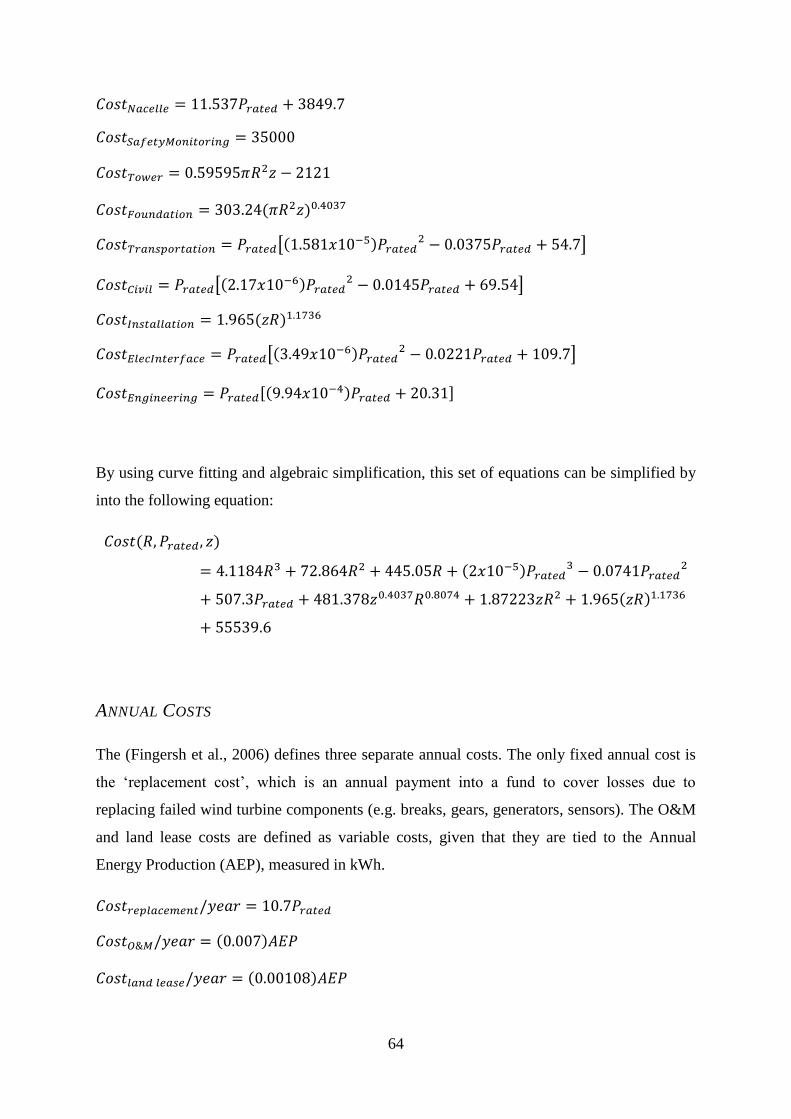
64
[
]
[
]
[
]
[ ]
By using curve fitting and algebraic simplification, this set of equations can be simplified by
into the following equation:
ANNUAL COSTS
The (Fingersh et al., 2006) defines three separate annual costs. The only fixed annual cost is
the ‘replacement cost’, which is an annual payment into a fund to cover losses due to
replacing failed wind turbine components (e.g. breaks, gears, generators, sensors). The O&M
and land lease costs are defined as variable costs, given that they are tied to the Annual
Energy Production (AEP), measured in kWh.

65
7.5. TURBINE REFERENCE NUMBERS
This section includes the list of turbines analysed in this study, sourced from (Helgason,
2012), with reference numbers as used in Figure 15. The table includes the model’s accuracy
in measuring each turbine, shown as NRMSE when comparing the modelled power curve
with the manufacturer’s specified power curve.
Table 12: Turbine reference list, including rotor radius and generator capacity, and NRMSE of comparison with modelled
power curve
Ref # Turbine Name Rotor Radius (m) Capacity (MW) Model NRMSE
1 AAER A1650 77m 1650kW 38.50 1.65 5%
2 AAER A1650 82m 1650kW 41.00 1.65 12%
3 Bonus 82.4m 2.3MW 41.00 2.31 8%
4 Bonus MkIV 44m 600kW 22.00 0.61 6%
5 Clipper C100 100m 2500kW 50.00 2.50 4%
6 Clipper C89 89m 2500kW 44.50 2.50 6%
7 Clipper C93 93m 2500kW 46.50 2.50 6%
8 Clipper C96 96m 2500kW 48.00 2.50 5%
9 Enercon E101 101m 3000kW 50.50 3.05 8%
10 Enercon E33 33.4m 330kW 16.50 0.34 8%
11 Enercon E44 44m 900kW 22.00 0.91 7%
12 Enercon E48 48m 800kW 24.00 0.81 8%
13 Enercon E53 52.9m 800kW 26.00 0.81 9%
14 Enercon E70 71m 2300kW 35.50 2.31 7%
15 Enercon E82 E2 82m 2000kW 41.00 2.05 12%
16 Enercon E82 82m 2300kW 41.00 2.35 11%
17 Enercon E82 82m 3000kW 41.00 3.02 9%
18 Gamesa G52 850kW 26.00 0.85 6%
19 Gamesa G58 850kW 29.00 0.85 6%
20 Gamesa G80 2.0MW 40.00 2.00 9%
21 Gamesa G83 2.0MW 41.50 2.00 8%
22 Gamesa G87 2.0MW 43.50 2.00 7%
23 Gamesa G90 2.0MW 45.00 2.00 7%
24 GE 1.6MW 50.00 1.60 5%
25 GE 1.5sl 77m 1500kW 38.50 1.50 5%
26 GE 2.5xl 100m 2500kW 50.00 2.50 3%
27 GE 3.6sl 111m 3600kW 55.50 3.60 4%
28 Leitwind LTW101m 3MW 50.00 3.00 5%
29 Leitwind LTW70 1.7MW 35.00 1.70 5%
30 Leitwind LTW70 2MW 35.00 2.00 4%
31 Leitwind LTW77m 1.5MW 38.50 1.50 4%
32 Leitwind LTW80 1.5MW 40.00 1.50 12%
33 Leitwind LTW80 1.8MW 40.00 1.80 12%
34 Nordex N100 2500kW 49.50 2.50 8%
35 Nordex N60 1.3MW 30.00 1.34 6%

66
36 Nordex N70 1.5MW 35.00 1.50 5%
37 Nordex N90 2500kW 45.00 2.51 6%
38 Nordex S70 1500kW 35.00 1.50 5%
39 Nordex S77 1500kW 38.50 1.50 4%
40 Siemens SWT 101m 2.3MW 50.50 2.30 7%
41 Siemens SWT 93m 2.3MW 46.50 2.30 8%
42 Siemens SWT 3.6MW 53.50 3.60 4%
43 Vestas V90 3MW 45.00 3.00 6%
44 Vestas 80m 2MW 40.00 2.00 10%
45 Vestas V 90 GridStreamer 2MW 45.00 2.00 7%
46 Vestas V52 850kW 26.00 0.85 5%
47 Vestas V82 1.65MW 41.00 1.65 9%

67
7.6. C++ CODE (EXCLUDING GA CODE IMPLEMENTATION)
The Genetic Algorithm code has been excluded from the appendix, as it is available at
(Garrett, 2013). Instead the code shown here is for a single iteration of the BEM theory and
Cost-Scaling model.
7.6.1. MAIN CODE /* TurbOpt.cpp: * Turbine selection program - * Uses BEM Theory and NREL Cost Scaling Model * To calculate performance of a wind turbine * That uses S809 aerofoils * At a given location */ #include "stdafx.h" #include "RotorProfiles.h" #include "BEMLoop.h" #include <iostream> #include <fstream> #include <cmath> #include <string> #include "TurbineCost.h" #include "Burfell.h" #include "LCOE.h" int main() { using namespace std; //Step 0: Initial Global Assumptions (GA variables noted with a '[ga]' at start of comment) double dB = 3; // Number of Blades (#) double dR = 37.4; // [ga] Rotor Length [metres] double dGenCap = 1738000; // [ga] Maximum Generator Capacity (W) int iHH = 70; // [ga] Hub Height (m) double dRho = 1.225; // Assumed density of air (kg/m3) double dEfficiency = 0.95; // Efficiency Assumed for gearbox and generator int iWindCutOut = 20; // Cutout speed for wind turbine int iWindCutIn = 5; // Cutin speed for wind turbine double alpha = 0.127; // Wind Shear Factor int iInvestPeriod = 20; // Investment period measured in years (for LCoE calculation) double dDiscountRate = 0.05; // Discount rate for future investments (for LCoE calculation) int iRPMmin = 12; // [ga] Set minimum rotor RPM for BEM theory loop int iRPMRange = 30; // [ga] Range of RPM speeds for wind turbine int iRPMmax = iRPMmin+iRPMRange; // Calculated maximum rotor RPM for BEM loop int iPitchMin = 0; // [ga] Set minimum rotor pitch angle for BEM theory loop int iPitchRange = 20; // [ga] Set range of pitch control for wind turbine int iPitchMax = iPitchMin+iPitchRange;// Calculated max pitch angle for BEM loop double dInflation = 0.298; // Inflation since 2002 (to 2013) //STEP 1: BEM THEORY CALCULATIONS // Initialize Power Curve array, 20 elements for velocity, each with [dPower,dThrust,iRPM,iPitch] double adPowerCurve[20][4] = { 0 }; //Runs BEM Theory modules and outputs resultant Power Curve to PCurve.csv BEMLoop(dB,dR,dGenCap,dRho,dEfficiency,adPowerCurve,iRPMmin,iRPMmax,iPitchMin,iPitchMax); //STEP 2: AEP CALCULATIONS //Enter 'Burfell.h' to check wind output based on 10min wind interval data and hub height, in kWh double dAEPBurf = Burfell(iHH,iWindCutOut,iWindCutIn,alpha,adPowerCurve, dRho);

68
//STEP 3: COST CALCULATIONS double dCostInitial; double dCostFixed; double dCostVariable; //Calls 'TurbineCost.h' and returns turbine costs TurbineCost(dB,dR,dGenCap,iHH,dAEPBurf,dCostInitial,dCostFixed,dCostVariable,dInflation); //STEP 4: KEY RESULT OUTPUT //output key results to screen cout << "KEY RESULTS" << endl; cout << "--------------------" << endl; cout << "AEP = " << dAEPBurf/1000000 << " GWh/year" << endl; cout << "Initial Cost = " << static_cast<int>(dCostInitial) << " USD" << endl; cout << "LCoE = ";
cout << LCOE(dCostInitial,dCostFixed,dCostVariable,iInvestPeriod,dDiscountRate,dAEPBurf)*1000; cout << " USD/MWh" << endl;
cout << "Capacity Factor = " << dAEPBurf / ((dGenCap/1000)*8766) << endl << endl; //output key results to 'Summary.csv' file ofstream outf("Summary.csv"); outf << "Initial Cost (USD),Fixed Cost (USD),Var. Cost (USD),AEP (GWh/yr)”;
outf << “,LCoE (USD/MWh),Cap Fac." << endl; outf << static_cast<int>(dCostInitial) << "," << static_cast<int>(dCostFixed);
outf << "," << static_cast<int>(dCostVariable); outf << "," << dAEPBurf/1000000 << ",";
outf << LCOE(dCostInitial,dCostFixed,dCostVariable,iInvestPeriod,dDiscountRate,dAEPBurf)*1000; outf << "," << dAEPBurf / ((dGenCap/1000)*8766) << endl; outf.close(); //end program return 0; }

69
7.6.2. BEM LOOP CODE //Module that receives wind turbine characteristics and returns a power curve //in the form of an array #ifndef BEMLoop_H #define BEMLoop_H #include <iostream> #include <fstream> #include <cmath> const double PI =3.141592653589793238462; void BEMLoop(double dB, double dR,double dGenCap,double dRho, double dEfficiency, double adPowerCurve[20][4], int iRPMmin, int iRPMmax, double iPitchMin, double iPitchMax) { using namespace std; //Define output file ofstream outf("PCurve.csv"); //Check that output file was created successfully, else write error message and terminate if (!outf) { cerr << "Uh oh, couldn't create PCurve.csv, try closing PCurve.csv if it is open." << endl; exit(1); } //Set loop parameters const int iii_max = 20; // Maximum Iteration Count (for convergence of a and a') const int iSections = 25; // blade sections: should be data points for r/R, C/R and twist minus 1 iRPMmin = 0; // Set min RPM to 0 //Initialize parameters (where required) double dRadius = 0.0; // Element Radius [r] (m) double dRadius_old = 0.0; // Stores the radius of the previous element (m) double dC = 0.0; // Element Chord Width [C] (m) double dTwist = 0.0; // Element Twist angle (in degrees) double dElementWidth = 0.0; // Element width [dr] (m) double dCL = 0.0; // Profile Lift Coefficient (-) double dCD = 0.0; // Profile Drag Coefficient (-) double dT = 0.0; // Incrememental thrust (N) double dM = 0.0; // Incremental moment (N.m) double da = 0.0; // Axial induction factor (-) double da_dash = 0.0; // Rotational induction factor (-) double dPhiRads = 0.0; // Flow Angle (radians) double dCn = 0.0; // Normal Blade Coefficient (-) double dCt = 0.0; // Tangential Blade Coefficient (-) double dMoment = 0.0; // Total Blade Moment (N.m) double dPower = 0.0; // Total Rotor power for given wind speed and settings (W) double dThrust = 0.0; // Total thrust force on the rotor (N) int iRPM = iRPMmin; // RPM counter (-) int iPitch = 0; // Pitch counter (-) //Begin loop for integer value of Wind Speed (1 to 25, as curve is flat or cut-out after 25 m/s) for(int iV = 1 ; iV < 21 ; iV++) { //Begin loop for RPM (min value to max value) for(iRPM = iRPMmin ; iRPM < iRPMmax+1 ; iRPM++) { double dGamma = (iRPM*2.0*PI)/60.0; //Angular velocity of blade tip double dTSR = (dGamma * dR) / iV; //Set upper-limit of TSR, to avoid wasteful calculations if(dTSR >11) break; //Begin loop for Pitch angle (min value to max value) for(iPitch = iPitchMin ; iPitch < iPitchMax+1 ; iPitch++) { double dPT[iSections];

70
//Reset key result parameters before new iteration of BEM algorithm dMoment = 0.0; dPower = 0.0; dThrust = 0.0; //Begin loop for blade elements from element 1 to 19 for(int iElement=1 ; iElement<iSections+1; iElement++) { //Step 1: Initialize a and a', typically a = a' = 0 da = 0.0; //a da_dash = 0.0; //a' //Store previous radius value dRadius_old = dRadius; //Initialize and define Prandtl Tip Loss coefficients double dPrandtl_f = 0.0; double dPrandtl_F = 0.0; //Begin loop for convergence of a and a' for given blade section for(int iii=1 ; iii< iii_max; iii++) { //Call formula from 'RotorProfiles.h' to update blade parameters from table ChordTwist(iElement, dR, dRadius, dC, dTwist, dElementWidth); //Step 2: Compute the flow angle (phi) using equation 6.7 dPhiRads = atan( ((1.0-da)*iV) / ((1.0+da_dash)*dGamma*dRadius) ); //Flow Angle [radians] //Step 3: Local Angle of Attack using equation 6.6 double dTheta = static_cast<double>(iPitch) + dTwist; //Local pitch [degrees] double dAlpha = (dPhiRads * 180.0)/PI - dTheta; //Local angle of attack [degrees] //Step 4: Determine Lift and Drag Coefficients from table //Look up Lift and Drag data values from table in 'RotorProfiles.h', and assign to params LiftDrag(dAlpha, dCL, dCD); //Chaviaropolous and Hansen correction (2000) double dChaviF = 0.0; if(dAlpha<15.0) dChaviF = 1.0; else if(dAlpha<25.0) dChaviF = 0.5 * (cos(PI*((dAlpha - 15.0)/10))+1); else dChaviF = 0.0; dCL += dChaviF*(2.2*pow(dC/dRadius,1.3)*pow(cos(dTwist),4.0)*(1.231 - dCL)); dCD += dChaviF*(2.2*pow(dC/dRadius,1.3)*pow(cos(dTwist),4.0)*(dCD - 0.005)); //Step 5: Compute the Normal and Tangential Coefficients (Equations 6.12 and 6.13) dCn = dCL * cos(dPhiRads) + dCD * sin(dPhiRads); //Normal coefficient dCt = dCL * sin(dPhiRads) - dCD * cos(dPhiRads); //Tangential coefficient //Step 6: Calculation of new a and a' (Equations 6.23 and 6.24) double dSigma = (dC * dB)/(2.0 * PI * dRadius); //Simplified Prandtl Correction 'f' and 'F' coefficients dPrandtl_f = (dB/2.0)*((dR - dRadius)/(dRadius*sin(dPhiRads))); dPrandtl_F = (cos(exp((-1.0*dPrandtl_f)/2.5))); //Calculate new a and a' values, using Prandtl Tip Loss and Glauret corrections double da_new = 0.0; if(da<0.2) da_new = 1.0/(4.0 * dPrandtl_F * ((sin(dPhiRads)*sin(dPhiRads))/(dSigma * dCn)) + 1.0); else { double dK = (4.0 * dPrandtl_F * (sin(dPhiRads)*sin(dPhiRads)))/(dSigma*dCn);
da_new = 0.5*(2.0+dK*(1.0-2*0.2)-pow(pow(dK*(1.0-2.0*0.2)+2,2)+4.0*(dK*0.2*0.2-1),0.5)); }

71
double da_dash_new= 1.0/(4.0 * dPrandtl_F * ((sin(dPhiRads)*cos(dPhiRads))/(dSigma * dCt)) - 1.0); //Exit conditions for loop //calculate error between new and old a values, to check loop double dError_a = da - da_new; double dError_a_dash = da_dash - da_dash_new; //Ensure error values are positive (i.e. remove sign) if(dError_a < 0.0) dError_a *= -1.0; if(dError_a_dash < 0.0) dError_a_dash *= -1.0; //sum errors in a and a' as a total error double dTotError = dError_a + dError_a_dash; //If errors are less than tolerance, exit loop, else update a and a' if(dTotError <0.00001) break; else { da = da_new; da_dash = da_dash_new; } } //Calculate the incremental thrust (dT) and tangential (dPT) forces of the element double dT = 0.5 * dRho * dB * ((iV*iV*(1-da)*(1-da))/(sin(dPhiRads)*sin(dPhiRads)))*dC*dCn*dElementWidth; dPT[iElement-1] = 0.5 * dRho * ((iV*(1-da)*dGamma*dRadius*(1+da_dash))/(sin(dPhiRads)*cos(dPhiRads)))*dC*dCt; //Add incremental thrust to total thrust force dThrust += dT; //Interpolate the incremental tangential forces to calculate the moment on the blade if(iElement>1) { //Calculate the slope 'M' and intercept 'X' for linear integration of moments double dCoeffM = (dPT[iElement-1] - dPT[iElement-2])/(dRadius-dRadius_old); double dCoeffX = (dPT[iElement-2] * dRadius - dPT[iElement-1] * dRadius_old) / (dRadius-dRadius_old); dMoment += (1.0/3.0) * dCoeffM * ( pow(dRadius,3.0) - pow(dRadius_old,3.0)) + 0.5 * dCoeffX * (pow(dRadius,2.0) - pow(dRadius_old,2.0)); } //End of BEM loop } //Multiply moment by number of rotor blades to find total rotor moment dMoment *= dB; //Calculate rotor power in Watts dPower = dMoment * dGamma * dEfficiency; //Make sure generation is below/at generator capacity if(dPower>dGenCap)
dPower=dGenCap; if(dPower>adPowerCurve[iV-1][0]) { adPowerCurve[iV-1][0] = dPower; adPowerCurve[iV-1][1] = dThrust; adPowerCurve[iV-1][2] = iRPM; adPowerCurve[iV-1][3] = iPitch; } //End of RPM Loop } //End of Pitch Angle loop }

72
//Raise the minimum RPM and Pitch to values of previous operating RPM and Pitch, to reduce wasteful calculations if(adPowerCurve[iV-1][2] > iRPMmin) iRPMmin = adPowerCurve[iV-1][2]-1; if(adPowerCurve[iV-1][3] > iPitchMin) iPitchMin = adPowerCurve[iV-1][3]-1; //Output Power Curve to '.csv' file outf << iV <<","<< adPowerCurve[iV-1][0] <<","<< adPowerCurve[iV-1][1] <<","<< adPowerCurve[iV-1][2] <<","<< adPowerCurve[iV-1][3] << endl; //End Wind Speed Loop } outf.close(); } #endif

73
7.6.3. S809 ROTOR PROFILE REFERENCE CODE //Module that receives the angle of attack and returns a vector with the interpolated Lift Coefficient //in the first value, and the Drag Coefficient in the second value #ifndef RotorProfiles_H #define RotorProfiles_H //Formula to look up Lift and Drag coefficients from a table based on a given alpha angle (in degrees) void LiftDrag(double alpha, double &dLift, double &dDrag) { // Find integer value above and below specified alpha, as int values required for look-up table int down = static_cast<int>(alpha); int up = static_cast<int>(alpha+1); //2D array, where entry 0 is alpha = -20 degrees;column A = CL, column B = CD (Ramsav,1996 p.B-5) double adLiftDrag[97][2] = {Data from Appendix 7.3}; //Return values for Lift & Drag for integer alpha values bounding actual alpha value double dLiftDown = adLiftDrag[6+down][0]; double dDragDown = adLiftDrag[6+down][1]; double dLiftUp = adLiftDrag[6+up][0]; double dDragUp = adLiftDrag[6+up][1]; //Linearly interpolate Lift and Drag values for alpha based on the values returned from the table dLift = ((dLiftUp - dLiftDown) / (up - down))*(alpha-down) + dLiftDown; dDrag = ((dDragUp - dDragDown) / (up - down))*(alpha-down) + dDragDown; //Lift and Drag values are returned to the main program through reference parameters } //Formula that looks up the radius ratio (r/R), chord ratio (C/R) and Twist at elements along the rotor //Based on values listed in a pre-defined table void ChordTwist(int iElement, double dR, double &dRadius, double &dC, double &dTwist, double &dElementWidth) { //3-Dimensional array where entry 0 is r = 0 metres, entry 20 is r=R metres; //Column A = Radius Ratio, column B = Chord Ratio, column C = twist angle (deg) (NREL,2000) double RadChordTwist[26][3] = {Data from Appendix 7.2}; dRadius = RadChordTwist[iElement][0]*dR; dC = dR*RadChordTwist[iElement][1]; dTwist = (RadChordTwist[iElement][2]+ RadChordTwist[iElement-1][2])/2.0; dElementWidth = dR*RadChordTwist[iElement][0] - dR*RadChordTwist[iElement-1][0]; } #endif

74
7.6.4. AEP CALCULATION CODE #ifndef Burfell_H #define Burfell_H #include <cmath> double Burfell(int iHH, int iWindCutOut, int iWindCutIn, double alpha, double adPowerCurve[20][4], double dRho) { //Burfell Wind Data 10min intervals static const double BurfellWind[52704] = {Wind Speed Data redacted due to confidentiality agreement}; //Contains temperature at a height of 10m above ground level at Burfell static const double BurfellTemp[52704] = {Temperature Data redacted due to confidentiality agreement}; //Set initial parameters double dV = 0.0; //Wind Speed read from Burfell data, used in iteration loop below double dP = 0.0; //Power at dV, used in iteration loop below double dTime = 10.0/60.0; //Time step for each data point (i.e. 10/60 hours) double dAEP = 0.0; //Annual Energy Production, returned by function double dElev = 100; //Assumed elevation at Burfell double dPress0 = 100600; //Air pressure at sea level [Pa] (Nawri, 2012) double dTemp0 = 278.5; //Air temperature at sea level [K] (Nawri, 2012) double dLt = 0.0063; //Terrain following temperature lapse rate [K/m] (Nawri, 2012) double dL = 0.0057; //Atmospheric temperature lapse rate [K/m] (Nawri, 2012) const int iRgas = 287; //Specific gas constant of dry air [J/K.kg] const double g = 9.81; //Gravitational accelleration constant [m/s2] double dTempHH = 0.0; //Temperature at hub height, initialized for loops below double dRhoAdj = 0.0; //Adjusted air density at hub height [kg/m3] for loops below //Air Density Correction: pressure calculation
double dPress = dPress0 * (pow(dTemp0 / (dTemp0 + (dLt * dElev)),g/(dLt*iRgas))) * (pow((dTemp0 + (dLt * dElev)) / (dTemp0 + (dLt * dElev)+(dL*iHH)),g/(dL*iRgas))); //Loop over all wind speed values and calculate power output for(int iii=0; iii <52703; iii++) { dV = BurfellWind[iii]; dTempHH = BurfellTemp[iii] + dL * (iHH - 10.0) + 273.15; //Temperature at Hub Height [K] dRhoAdj = dPress / (iRgas*dTempHH); //adjusted air density value //Wind shear correction, using alpha value and hub height dV *= pow((static_cast<double>(iHH)/10.0),alpha); //Check if wind speed is within operational range if(dV > iWindCutOut || dV < iWindCutIn) { dAEP += 0; continue; } else if(dV > 20) { dP = adPowerCurve[19][0]; dAEP += dP * dTime * (dRhoAdj/dRho); continue; } //Linearly interpolate output from BEM power curve int iVDown = static_cast<int>(dV); int iVUp = static_cast<int>(dV+1); dP = ((adPowerCurve[iVUp-1][0] - adPowerCurve[iVDown-1][0])/(iVUp-iVDown))*(dV-iVDown) + adPowerCurve[iVDown-1][0]; dAEP += dP * dTime * (dRhoAdj/dRho); } dAEP /= 1000; //Convert dAEP from Wh to kWh return dAEP; } #endif

75
7.6.5. TURBINE COST CODE //'TurbineCost.h' calculates the cost of the defined turbine // and returns Initial, Fixed and Variable costs in 2013 USD #ifndef TurbineCost_H #define TurbineCost_H #include <cmath> int TurbineCost(double dB, double dR,double dGenCap, int iHH, double dAEP, double &dCostInitial, double &dCostFixed, double &dCostVariable, double dInflation) { //Convert Generator Capacity from Watts to kiloWatts dGenCap /= 1000.0; //Use the Fingersh WINDPACT method, gives cost in 2002 USD (Fingersh,2006) //INITIAL COSTS
dCostInitial= 4.1184*pow(dR,3)+72.864*pow(dR,2)+445.05*dR+(2.0E-5)*pow(dGenCap,3)-0.0741*pow(dGenCap,2)+507.3*dGenCap+481.378*pow(iHH,0.4037)*pow(dR,0.8074)+1.87223*iHH*pow(dR,2)+1.965*pow(iHH*dR,1.1736)+55539.6; //ANNUAL COSTS //Annual Replacement Cost double dAnnualRepFix = 10.7 * dGenCap; //Operations and Maintenance double dOMVar = 0.007 * dAEP; //Land Lease Costs double dLLVar = 0.00108 * dAEP; dCostFixed = dAnnualRepFix; dCostVariable = dOMVar + dLLVar; //Adjustment factor to bring cost estimates in line with reality (based on real costs at Burfell) double dInitialAdj = 2.4022; //Adjust for inflation dCostInitial *= (1+dInflation)*dInitialAdj; dCostFixed *= (1+dInflation); dCostVariable *= (1+dInflation); return 0; } #endif

76
7.6.6. LEVELIZED COST OF ENERGY CODE //Module that receives initial and annual costs, AEP and discount rate //And returns the Levelized Cost of Energy (LCoE) #ifndef LCOE_H #define LCOE_H #include <cmath> double LCOE(double dCostInitial,double dCostFixed,double dCostVariable,int iInvestPeriod, double dDiscountRate, double dAEP) { //Initialize loop parameters double dAnnualSum = 0.0; //Sum of Levelized annual costs double dAEPSum =0.0; //Sum of Levelized annual electricity production //Loop for investment period (lifetime of investment in years) for(int iii = 1 ; iii < iInvestPeriod ; iii++) { dAnnualSum += (dCostFixed+dCostVariable) / pow((1.0+dDiscountRate),iii); dAEPSum += dAEP / pow((1.0+dDiscountRate),iii); } //Return LCoE return ((dCostInitial + dAnnualSum) / dAEPSum); } #endif