Embed Size (px)
Citation preview

Wind Loads on Bridges
Analysis of a three span bridge based on theoretical
methods and Eurocode 1
M. Sajad Mohammadi
Rishiraj Mukherjee
June 2013TRITA-BKN. Master Thesis 385, 2013
ISSN 1103-4297ISRN KTH/BKN/EX-385-SE

.
Examiner and supervisor: Prof. Raid Karoumi
@M. Sajad Mohammadi ([email protected]), 2013@Rishiraj Mukherjee ([email protected]), 2013Royal Institute of Technology (KTH)Department of Civil and Architectural EngineeringDivision of Structural Design and BridgesStockholm, Sweden, 2013
Abstract
The limitations lying behind the applications of EN-1991-1-4, Eurocode1, actionson structures-general actions-wind load-part 1-4, lead the structural designers to agreat confusion. This may be due to the fact that EC1 only provides the guidancefor bridges whose fundamental modes of vibration have a constant sign (e.g. simplysupported structures) or a simple linear sign (e.g. cantilever structures) and thesemodes are the governing modes of vibration of the structure. EC1 analyzes onlythe along-wind response of the structure and does not deal with the cross wind re-sponse. The simplified methods that are recommended in this code can be used toanalyze structures with simple geometrical configurations. In this report, the ana-lytical methods which are used to describe the fluctuating wind behavior and predictthe relative static and dynamic response of the structure are studied and presented.The criteria used to judge the acceptability of the wind load and the correspondingstructural responses along with the serviceability considerations are also presented.Then based on the given methods the wind forces acting on a continuous bridgewhose main span is larger than the 50 meters (i.e. > 50 meter requires dynamicassessment) is studied and compared with the results which could be obtained fromthe simplified methods recommended in the EC1.
Key words: Wind load, dynamic response of a continuous bridge, theoretical meth-ods, Eurocode 1, vortex shedding, aerodynamic and aeroelastic instabilities, Naturalfrequencies.


Sammanfattning
De begransningar som ligger bakom tillampningarna av Eurokod 1: Laster pa barverk-Del 1-4: Allmanna laster – Vindlast leder, byggnadskonstruktorer till stor forvirring.Detta beror eventuellt pa grund av det faktum att Euokod 1 bara ger vagledning forbroar vars huvudsakliga svangningsmoder har konstant tecken eller enkelt linjarttecken och att dessa ar de dominerande svaningsmoder av barverk. Eurocod 1analyserar endast hur barverk ror sig i vindriktningen. De forenklade metodersom rekommenderas i denna kod tillampas for att analysera de barverk som harenkla geometriska konfigurationer. I denna rapport diskuteras och redovisas deanalytiska metoderna som anvands for att beskriva det varierande vindbeteendetoch berakningar av relativ statisk och dynamisk respons av barverket. De kriteriersom anvands for att bedomma godtagbarheten av vindlasten och dess motsvarandepaverkan pa barverket, tillsammans med overvaganden kring funktionsduglighet,presenteras ocksa. Baserat pa de givna metoderna studeras och jamfors vindlastersom verkar pa en kontinuerlig bro vars storsta spann ar storre an 50 meter (dvs.> 50 meter kraver dynamisk bedomning), med de resultat som kan erhallas fran deforenklade metoderna som rekommenderas i EC1.
Sokord: Vindlast, dynamisk respons av en kontinuerlig bro, teoretiska metoder, Eu-rokod 1, virvelavlosning, aerodynamiska och aeroelastisk instabilitet, egenfrekvens..


Acknowledgements
We would like to express our sincere gratitude to our project guide Prof. RaidKaroumi for his valuable comments, remarks and suggestions throughout the dura-tion of the master thesis. Furthermore we would like to thank Ali Farhang, MarcoAndersson, Jens Haggstrom and Jesper Janzon-Daniel of Ramboll AB for providingus with the relevant data and information required for the thesis. Also, we wouldlike to thank Johan Jonsson of Trafikverket for his guidance and comments.We would like to express our deepest appreciation to all the faculty members ofthe school of Architecture and Built Environment, KTH who imparted us with theknowledge and skills required for the successful completion of the project.


Contents
1 Introduction 5
2 Wind load 72.1 Wind load chain . . . . . . . . . . . . . . . . . . . . . . . . . . . . . . 72.2 The atmospheric boundary layer . . . . . . . . . . . . . . . . . . . . . 8
2.2.1 The roughness length . . . . . . . . . . . . . . . . . . . . . . 82.3 Mean wind velocity- wind profile(homogenous terrain) . . . . . . . . . 8
2.3.1 The logarithmic profile . . . . . . . . . . . . . . . . . . . . . 92.3.2 Corrected logarithmic profile . . . . . . . . . . . . . . . . . . 92.3.3 Power law profile . . . . . . . . . . . . . . . . . . . . . . . . . 10
2.4 Wind turbulence . . . . . . . . . . . . . . . . . . . . . . . . . . . . . 102.4.1 Standard deviation of the turbulence components . . . . . . . 102.4.2 Time scales and integral length scales . . . . . . . . . . . . . . 112.4.3 Power-spectral density function . . . . . . . . . . . . . . . . . 132.4.4 correlation between turbulence at two points . . . . . . . . . . 16
2.5 Static wind load . . . . . . . . . . . . . . . . . . . . . . . . . . . . . . 162.5.1 Total wind load on structure- Davenport’s model . . . . . . . 17
3 Dynamic response of structures to the wind load 213.1 Along-Wind Response . . . . . . . . . . . . . . . . . . . . . . . . . . 21
3.1.1 Single degree of freedom . . . . . . . . . . . . . . . . . . . . . 213.1.2 The Along-wind response of bluff bodies . . . . . . . . . . . . 243.1.3 Design procedure for mode shapes with constant sign . . . . . 28
3.2 Cross-wind vibtrations induced by vortex shedding . . . . . . . . . . 303.3 Bridge aerodynamics and wind-induced vibrations . . . . . . . . . . . 34
3.3.1 Flutter . . . . . . . . . . . . . . . . . . . . . . . . . . . . . . . 363.3.2 Buffeting . . . . . . . . . . . . . . . . . . . . . . . . . . . . . . 393.3.3 Galloping . . . . . . . . . . . . . . . . . . . . . . . . . . . . . 42
4 Wind Load on Bridges based on Eurocode1 454.1 General . . . . . . . . . . . . . . . . . . . . . . . . . . . . . . . . . . 45
4.1.1 Distinction between principles and application rules . . . . . . 464.1.2 Definitions . . . . . . . . . . . . . . . . . . . . . . . . . . . . . 46
4.2 Design situation . . . . . . . . . . . . . . . . . . . . . . . . . . . . . . 474.2.1 Persistent situations . . . . . . . . . . . . . . . . . . . . . . . 484.2.2 Transient situations . . . . . . . . . . . . . . . . . . . . . . . . 48
2

Contents 3
4.2.3 Accidental situations . . . . . . . . . . . . . . . . . . . . . . . 484.2.4 Fatigue situations . . . . . . . . . . . . . . . . . . . . . . . . . 48
4.3 Modeling of wind actions . . . . . . . . . . . . . . . . . . . . . . . . . 494.4 Wind Velocity and Wind Pressure . . . . . . . . . . . . . . . . . . . . 49
4.4.1 Basic wind velocity . . . . . . . . . . . . . . . . . . . . . . . . 504.4.2 Mean wind . . . . . . . . . . . . . . . . . . . . . . . . . . . . 504.4.3 Wind turbulence . . . . . . . . . . . . . . . . . . . . . . . . . 504.4.4 Wind action . . . . . . . . . . . . . . . . . . . . . . . . . . . . 51
4.5 Structural factor (cs.cd) . . . . . . . . . . . . . . . . . . . . . . . . . . 514.6 Wind actions on bridges . . . . . . . . . . . . . . . . . . . . . . . . . 52
4.6.1 Force coefficients . . . . . . . . . . . . . . . . . . . . . . . . . 534.6.2 Force in x-direction- simplified method . . . . . . . . . . . . . 534.6.3 Wind forces on bridge decks in z-direction . . . . . . . . . . . 544.6.4 Wind forces on bridge decks in y-direction . . . . . . . . . . . 544.6.5 Wind effects on piers . . . . . . . . . . . . . . . . . . . . . . . 54
4.7 Annexes . . . . . . . . . . . . . . . . . . . . . . . . . . . . . . . . . . 54
5 Finite Element Modelling 555.1 LUSAS FEM . . . . . . . . . . . . . . . . . . . . . . . . . . . . . . . 55
5.1.1 Geometry . . . . . . . . . . . . . . . . . . . . . . . . . . . . . 555.1.2 Cross-sections . . . . . . . . . . . . . . . . . . . . . . . . . . . 605.1.3 Foundations . . . . . . . . . . . . . . . . . . . . . . . . . . . . 615.1.4 Materials . . . . . . . . . . . . . . . . . . . . . . . . . . . . . 615.1.5 Element interactions . . . . . . . . . . . . . . . . . . . . . . . 635.1.6 Finite element modeling in LUSAS . . . . . . . . . . . . . . . 635.1.7 Analysis of different boundary conditions . . . . . . . . . . . . 66
5.2 MATLAB FEM . . . . . . . . . . . . . . . . . . . . . . . . . . . . . . 70
6 Analysis and Results 726.1 Natural frequencies and Mode shapes . . . . . . . . . . . . . . . . . . 72
6.1.1 Results from LUSAS . . . . . . . . . . . . . . . . . . . . . . . 726.1.2 Results from Matlab . . . . . . . . . . . . . . . . . . . . . . . 80
6.2 Power spectral density function . . . . . . . . . . . . . . . . . . . . . 806.2.1 Deck . . . . . . . . . . . . . . . . . . . . . . . . . . . . . . . . 846.2.2 Piers . . . . . . . . . . . . . . . . . . . . . . . . . . . . . . . . 86
6.3 Response-influence function . . . . . . . . . . . . . . . . . . . . . . . 866.3.1 Deck . . . . . . . . . . . . . . . . . . . . . . . . . . . . . . . . 866.3.2 Piers . . . . . . . . . . . . . . . . . . . . . . . . . . . . . . . . 86
6.4 Wind Load Analysis . . . . . . . . . . . . . . . . . . . . . . . . . . . 876.4.1 Determination of Gust factor . . . . . . . . . . . . . . . . . . 876.4.2 Determination of Maximum Wind Load on the Structure . . . 89
6.5 Vortex shedding and Aeroelastic instabilities . . . . . . . . . . . . . . 906.5.1 Vortex shedding . . . . . . . . . . . . . . . . . . . . . . . . . . 906.5.2 Galloping . . . . . . . . . . . . . . . . . . . . . . . . . . . . . 906.5.3 Divergence and Flutter Response of the Bridge Deck . . . . . 90

4 Contents
7 Conclusion 97
References 99
Appendices 102
A Mass Participation Factor 103
Appendices 105
B MATLAB Code 106


Chapter 1
Introduction
Wind load is one of the structural actions which has a great deal of influence onbridge design. The significant role of wind loads is more highlighted after it causednumbers of bridge structures to either collapse completely, e.g., Tacoma NarrowsBridge (1940) or experience serviceability discomforts e.g. Volgograd bridge (2010).Massive researches and studies have been carried out all over the world in order toanalyze and model the fluctuating wind behavior and its relative static and dynamicinteractions with the bridge components and the corresponding structural responsesto the turbulent wind load.
The nature of the wind load is dynamic. This means that its magnitude varieswith respect to time and space. As a result, analysis and modeling of such a loadand its relative effects on structure may be quite complex and require substantialknowledge in mathematics, computational fluid dynamics and structural analysis.The EN-1991-1-4 or Eurocode 1 and SS-EN-1991-1-4(2005) are the standard codesfor the designers to evaluate both the wind forces acting on the surface of thestructure and the corresponding static and dynamic response of the structures. SS-EN-1991-1-4(2005) contains the Swedish annex which points out which clauses inthe EN-1991-1-4 may or may not be used in Sweden. The mentioned standard codehas simplified the complex nature of the wind load and its corresponding effectson the bridge structures by suggesting some simplified methods to model the windphenomena and also recommends some simplified methods to determine the staticand dynamic response of structures. However, great attention must be paid whileusing the mentioned guidance as one may require knowledge of the background andlogics applied behind the given simplifications and the corresponding assumptionsand limitations to assure that the results represent the actual situations in the field.
The limitations behind the applications of the EN-1991-1-4, Eurocode1, actionson structures-general actions-wind load-part 1-4, lead the structural designers to agreat confusion. This may be due to the fact that, EC1 provides only the guid-ance for the bridges whose fundamental mode of vibrations have constant sign (e.g.simply supported structures) or a simple linear sign (e.g. cantilever structures) andthese modes are the governing mode of vibrations of the structure; it analyzes onlythe along-wind response of the structure and not the cross wind response and the
5

6 Introduction
simplified methods recommended in this code are covering only the structures withsimple geometrical configurations.
In this report, the analytical methods which are used to describe the fluctuatingwind behavior and predict the relative static and dynamic response of the structuresalong with the effect of serviceability criteria which influence the performance, arestudied and presented in the following chapters. Then based on the given methodsthe wind forces acting on a continuous bridge whose main span is larger than the50 meters (i.e. > 50 meter requires dynamic assessment) is studied and comparedwith the results which could be obtained from the simplified methods recommendedin the EC1.
In chapter 1, the wind characteristics, wind phenomena, basic wind velocity,mean wind velocity, turbulence, methods to determine the corresponding wind spec-tral density functions and static wind loads are described. In chapter 2 the corre-sponding dynamic response of the structure against the fluctuating wind load arediscussed. The vortex shedding and aerodynamic instabilities are also described inthis chapter. Chapter 3 is based on the EN-1991-1-4 and SS-EN-1991-1-4(2005)specifications and how the Eurocode 1 deals with the wind actions on bridge struc-tures. Chapter 4 describes the finite element analysis of the given continuous bridgeand modeling of the bridge structure in order to determine its relevant natural fre-quencies and carry out a dynamic assessment of the bridge. Chapter 5 representsthe analytical calculation of the wind loads acting on the bridge structure based onthe theoretical methods and the final conclusion is given in the chapter 6. The cor-responding tables of mass participation factors, sum mass participations obtainedfrom LUSAS and MATLAB code are given in appendix A and B respectively.

Chapter 2
Wind load
2.1 Wind load chain
Wind load and the wind response of the structure relation is illustrated in the formof a chain by A.G. Daveport, which draws the attentions towards the significantrole of each and every factor in the given chain while designing a safe and stablestructure against wind load which is shown below.
Figure 2.1: Wind load chain, suggested by A.G. Daveport
Davenport’s approach describes that the wind loading on the structures is de-termined by a combined effect of the wind climate which needs to be calculatedstatistically; the local wind exposure which depends on the terrain roughness and to-pography; aerodynamic characteristics of the structures which depend on the shapeof the structure; dynamic effect i.e. the wind load magnitude (potential) increasesdue to the wind-induced resonant vibrations. Stiff structures may vibrate in differentways when subjected to wind loading. e.g. along-wind vibrations called buffetingmay occur with the turbulence[15]. Slender structures are especially susceptible tocross-wind vibrations caused by vortex shedding, and within certain ranges of windvelocities, wind load perpendicular to the wind direction may be in resonance withthe structure. Cable supported bridges and some other structures may vibrate whenvertical and torsional movements are coupled. This phenomenon, known as classicalflutter, occurs only at high wind velocities. However, bridges where flutter is likelyto occur must be studied in wind-tunnel experiments, as flutter can cause the struc-ture to collapse completely. And finally the clear criteria needs to be establishedto judge acceptability of the predicted wind load and the corresponding responses.This includes the effect of the wind on the entire structure, each component, exteriorenvelope and various serviceability considerations which influence the performance
7
8 Wind load
and which determine the habitability [9].
2.2 The atmospheric boundary layer
The wind velocity and its corresponding direction near the ground surface changeswith respect to the variation of height. When wind is approaching the offshoreits velocity reduces close to the ground as the ground surface tends to reduce thewind speed and this effect is minimized as the height of the wind increases from theground surface. This effect exists up to a height of 1000 meters which is known asheight of geostrophic wind above the atmospheric layer [7].
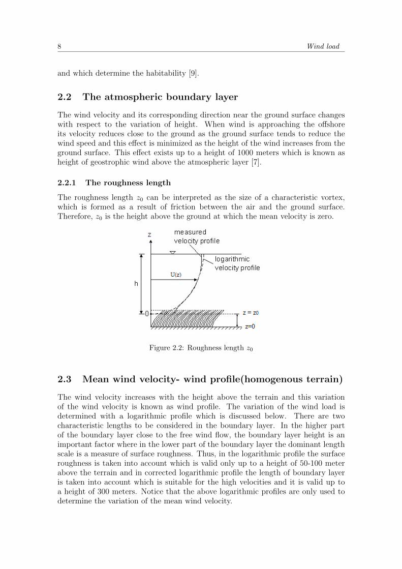
2.2.1 The roughness length
The roughness length z0 can be interpreted as the size of a characteristic vortex,which is formed as a result of friction between the air and the ground surface.Therefore, z0 is the height above the ground at which the mean velocity is zero.
Figure 2.2: Roughness length z0
2.3 Mean wind velocity- wind profile(homogenous terrain)
The wind velocity increases with the height above the terrain and this variationof the wind velocity is known as wind profile. The variation of the wind load isdetermined with a logarithmic profile which is discussed below. There are twocharacteristic lengths to be considered in the boundary layer. In the higher partof the boundary layer close to the free wind flow, the boundary layer height is animportant factor where in the lower part of the boundary layer the dominant lengthscale is a measure of surface roughness. Thus, in the logarithmic profile the surfaceroughness is taken into account which is valid only up to a height of 50-100 meterabove the terrain and in corrected logarithmic profile the length of boundary layeris taken into account which is suitable for the high velocities and it is valid up toa height of 300 meters. Notice that the above logarithmic profiles are only used todetermine the variation of the mean wind velocity.

Mean wind velocity- wind profile(homogenous terrain) 9
2.3.1 The logarithmic profile
The friction velocity u∗ is defined by the following formula:
u∗ =
√τ
ρ(2.1)
Where τ is the shear stress at the ground surface and ρ is the air density. Close tothe ground, the velocity gradient dU(z)/dz depends upon τ and ρ and the height zabove the ground. Based upon a dimensional analysis, a differential equation for themean wind velocities can be formulated and if there is a long , flat terrain upstream,its solutions lead to the following expression for the logarithmic profile.
U(z) =u∗κ. ln
z
z0(2.2)
Where κ is von Karaman’s constant (κ ∼ 0.4) and z0 is called the roughnesslength. Eurocode 1 uses the logarithmic profile for the mean wind velocity up to200 meter above the ground level. The corresponding value of the z0 is given by thefollowing table 4.1 in EC1.
2.3.2 Corrected logarithmic profile
The expression (2.2) for logarithmic profile is not valid at very high altitude aboveground. Harris and Deaves (1980) have suggested the following formula.
U(z) = u∗κ.[ln z−d
z0+ 5.75a− 1.88a2 − 1.33a3 + 0.25a4]
Where the actual, effective height, z − d, is normalized by the gradient height zgwhen calculating the non-dimensional argument a.
a =z − dzg
(2.3)
The gradient height zg is given by :
zg =u∗
6.fc(2.4)
Where fc is the coriolis parameter and given as follows:
fc = 2.Ω. sinλ (2.5)
Where Ω is the angular velocity of the earth (2.π/24hours = 7.27.10−5rad/sec)and λ is the latitude.

10 Wind load
2.3.3 Power law profile
There is another empirical formula which is used in Canadian code NBC 1990, whichis expressed as:
U(z) = U(zref ).(z
zref)α (2.6)
Where, zref is the reference height in m, α is given in tabular form in the codewhich depends on the terrain category.
2.4 Wind turbulence
The wind in the boundary layer is naturally turbulent i.e. the flow varies randomlyfrom interval of a second to several minutes. The statistical methods are used todescribe the turbulent flow. A Cartesian coordinate system is applied, with thex-axis in the direction of the mean wind velocity (along wind direction), the y-axishorizontal (cross wind direction) and the z –axis vertical , positive upwards. Thevelocities at a given time t are formulated as:
Longitudinal − direction : U(z) + u(x, y, z, t) (2.7)
Lateral − direction : v(x, y, z, t) (2.8)
V ertical − direction : w(x, y, z, t) (2.9)
Where the U(z) is the mean velocity and depends only on the height above theground . u, v, w describe the fluctuating part of the wind field, and can be treatedmathematically as stationary, stochastic processes with a zero mean value.
A stochastic process is referred to a phenomenon if the phenomenon has beenmeasured/recorded on many occasions during sufficiently long interval of time, thencertain statistical properties of the phenomenon can be deduced. Statistical prop-erties may also be based on mathematical modeling of the phenomenon. The phe-nomenon itself is then described as a stochastic process, and any measured sampleduring a time period is called a realization of the stochastic process.
Expected values of the process itself, or combinations of the process at differenttimes or positions, can be derived from the measurements or mathematical model-ing. If theses expected values are time independent, and if the correlation betweenvalues at different times only depend on time differences, then the process is calledstationary.
The figure below illustrates the variation of the mean wind velocity with re-spect to the height above the ground level and the time along with the turbulencecomponent u(z,t).
2.4.1 Standard deviation of the turbulence components
The standard deviations of the turbulence components in the wind direction u, inhorizontal v, and in vertical direction w, up to a height of 100-200m above homoge-neous terrain are approximately

Wind turbulence 11
Figure 2.3: Simultaneous wind velocities in the wind direction at different heights abovethe ground (left) and time(right).
σu = A.u∗ (2.10)
σv ≈ 0, 75.σu (2.11)
σw ≈ 0, 5.σu (2.12)
Where the constant A ≈ 2.5ifz0 = 0.05m and A ≈ 1.8ifz0 = 0.3mThe turbulence intensity Iu(z) for the long-wind turbulence component u at
height z is defined as:
Iu(z) =σu(z)
U(z)(2.13)
Where σu(z) is the standard deviation of the turbulence component u and U(z)is mean vind velocity, both at height z. For flat terrain, the turbulence intensity isapproximately given by:
Iu(z) =1
ln zz0
(2.14)
Where z0 is the roughness length and σu/u∗ is assumed to be 2.5 .Up to 100-200 m above the ground, it is usually reasonable to assume that
the turbulence components are distributed normally with a zero mean value andstandard deviations as given above. However this does not hold for the tails ofthe distribution, i.e. when the turbulence components are outside a range of ±3standard deviations. In this case the assumption of normal distribution may leadto significant errors.
2.4.2 Time scales and integral length scales
Here in this section two correlation functions are introduced. The autocorrelationfunctions ρTu (z, τ) which is defined as the normalized mean value of the product ofthe turbulence component u at the time t and u at the time t+ τ ,
12 Wind load
ρTu (z, τ) = Eu(x, y, z, t).u(x, y, z, t+ τ)/σ2u(z) (2.15)
The function indicates that how much information a measurement of the turbu-lence component u(x, y, z, t) in the mean wind direction will provide about the valueof u(x, y, z, t+ τ) measured at a time τ later at the same place [9].
The autocorrelation function depends only on height z above ground and on timedifference τ due to the assumption of the horizontal homogeneous flow. u may besaid to have a characteristic time of memory, the so called time scale T (z). In otherwords, time scale represents how long the turbulence is being measured i.e. the totaltime period and τ is the time segments inside the interval of time scale. One of theimportant measurements of u taken at time t give a great deal of information aboutu at the time τ later if τ T (z) , but only little information, if τ T (z). theformal definition of time scale T (z) is
T (z) =
∫ ∞0
ρTu (z, τ) dτ (2.16)
ρTu (z, τ) = exp(− τ
T (z)) (2.17)
Lxu =
∫ ∞0
ρu(z, rx)drx (2.18)
Integral length scale is a measure of the sizes of the vortices in the wind, or inother words the average size of a gust in a given direction. According to Taylor’shypothesis, ρu(z, rx) = ρTu (z, τ)forrx = U(z).τ indicating that the longitudinalintegral length scale is equal to the time scale multiplied by the mean velocity,Lxu(z) = U(z)T (z).
Full scale measurements are used to estimate integral length scales. Howeverresults show extensive scatter originating mainly from the variability of the lengthand degree of stationary of the records being analyzed. The integral length scalesdepend upon the height z above ground and on the roughness of the terrain, i.e.roughness length z0. The wind velocity may also influence the integral length scalesat site. Counihan(1975), has suggested the following purely empirical expression forthe longitudinal integral length at height z in the range of 10-240m.
Lxu = Czm (2.19)
Where C and m depend on roughness length z0 which can be determined graph-ically by referring to the Counihan(1975).
Lyu ≈ 0.3Lxu (2.20)
Lzu ≈ 0.2Lxu (2.21)

Wind turbulence 13
2.4.3 Power-spectral density function
Power spectral density function is a dimensionless function which describes the fre-quency in a distributed form for the turbulent along-wind velocity component, u.There are different suggestions to determine these functions. The most commonand frequently used power spectral density functions are discussed here in this sec-tion. The frequency distribution of the turbulent along-wind velocity component uis described by the non-dimensional power spectra density function Rn(z, n) definedas:
RN(z, n) = nSu(z, n)/σ2u(z) (2.22)
Where n is the frequency in Hertz and Su(z, n) is the power spectrum for thealong-wind turbulence component. Turbulent energy is generated in large eddies(low frequencies) and dissipated in small eddies (high frequencies). In the intermedi-ate region, called the inertial sub-range the turbulent energy production is balancedby turbulent energy dissipation, and the turbulent energy spectrum is independentof the specific mechanisms of generation and dissipation. For most of the structuresexcept flexible offshore structures (as these structures have very low frequencies),the spectral values for frequencies within this range (inertial sub-range) are the mostimportant.
Based on Tylor’s hypothesis frozen turbulence and considering the frequenciesin the inertial sub-range, the non-dimensional power spectrum function RN is givenby:
RN(z, n) = A.f−2/3L (2.23)
Where A is a constant depending slightly on height and fL = nLxu(z)/U(z) andLxu(z) is a height dependent length scale of turbulence. The constant A should beobtained based on full-scale spectral density functions measured at different height,preferably using the integral length scale in the high-frequency calculated by equa-tion above i.e. L(z) = Lxu(z). According to ESDU 85020, a function decreases withincreasing height and for a structure up to a height of 200-300 m, spectral functionsare obtained within accuracy 5% accuracy using A = 0, 14 for all heights assum-ing L(z) = Lxu(z). Different suggestions or methods to determine the power spectradensity functions in the literatures are Von Karman, Harris, Davenport and Kaimal.
Kaimal spectra density function for longitudinal turbulence component
Kaimal el al. (1972) [17] suggests the following spectral density function which iscommonly used:
Rn(z, n) = 2.3λfz/(1 + λfz)5/3 (2.24)
Where, λ = 50, the non-dimensional parameter used to locate the maximumvalue of the spectral density obtained for fz = f(z,max) = 3/2λ. The integrallength scale Lxu obtained using the spectral density function is equal to:

14 Wind load
Lxu(z) = U(z)T (z) =U(z)Su(z, 0)
4σ2u(z)
= λz/6 (2.25)
The above equation is appropriate for the height higher than 50 meters, forstructures lower than this height instead of fz in the spectral density function thefollowing equation needs to be used:
fL = nLxu(z)/U(z) (2.26)
Therefore we obtain the following expression which is used in Eurocode1:
Rn(z, n) = 6.8fL/(1 + 10.2fL)5/3 (2.27)
Where, fL is calculated from expression (2.25). The spectral density functionmay be used for the structures whose fundamental frequency of vibration is higherthan the lower end of the inertial sub-range. It gives an accurate representation ofthe turbulent fluctuations in the frequency range of interest for most structures.
Von Karman spectra density function for longitudinal turbulence component
Von Karman (1948) [36] has suggested the following expression for the the spectraldensity function:
Rn(z, n) = 4fL/(1 + 70.8f 2L)5/6 (2.28)
The above expression is used by the Swedish annex.
Davenport (1967) spectra density function for longitudinal turbulence compo-nent
Rn(z, n) = 2f 2L/3(1 + f 2
L)4/3 (2.29)
The only difference in this expression is that the function is based on the fL =nL/U(z), where and L ≈ 1200m [6].
Harris (1970) spectra density function for longitudinal turbulence component
Rn(z, n) = 2f 2L/3(2 + f 2
L)5/6 (2.30)
With non-dimensional frequency fL = nL/U(z), where and L ≈ 1800m [14]. Acomparison is made between the suggested functions which is shown in Figure 2.4.The fuctions are based on the integral length scale of Lxu(z) = 180m. It can beobserved that Davenport gives the highest power spectra and Von Karman giveshigher power spectral than the Kaimal( Eurocode1) but after frequency of 1 it isvice versa.
The Swedish annex suggests the value of integral length Lxu(z) = 150m. There-fore, corresponding spectral power density function is shown in Figure 2.5.
It can be observed that Von Karman gives a higher power spectra than theKaimal spectra function but for frequencies higher than 1 the power spectra obtainedby Kaimal(Eurocode1) is higher.

Wind turbulence 15
Figure 2.4: Power-spectral density functions for longitudinal turbulence component forLxu(z) = 180m.
Figure 2.5: Power-spectral density functions for longitudinal turbulence component forLxu(z) = 150m.

16 Wind load
Power spectra of lateral and vertical turbulence components are approximatelygiven by [28].
nSv(z, n)
u2∗=
15fz(1 + 9.5fz)5/3
(2.31)
nSw(z, n)
u2∗=
3.36fz(1 + 10fz)5/3
(2.32)
2.4.4 correlation between turbulence at two points
Davenport [8] suggested on the emperical basis the relaions between two turbulencepoint having distances ry and rz in horizontal and vertical dimensions (horizontalstructures) the following expression:
ϕu(ry, rz, n) = exp(− nU
√(Cyry)2 + (Czrz)2) (2.33)
Where Cy and Cz are the decay constants and they are determined using fullscale measurements.
2.5 Static wind load
In most of the structures the wind-induced resonant vibrations may be negligibleand the wind responses can be determined using the procedures applicable for staticloads. The wind load calculation is performed using the probabilistic methods andstochastic process. This means that the wind has a mean wind value and a stan-dard deviation. The peak factor kp is used to include the effect of the highest meanwind load taking place within the measured period of time (i.e. 10 min.). Turbu-lence gives a fluctuating contribution to the wind load which depends on structuralgeometry and other parameters. Therefore wind always fluctuates when acting onstructure or the structural components.
The characteristic wind load is the wind load with a mean wind value of mux orFmax and standard deviation of σF obtained within a particular time i.e. 10 minuteswhich is shown in the equation 2.34. The response of the structure to the charac-teristic wind load is also expressed as the characteristic response of the structurehaving mean response value and standard deviation. The static load that generatesa characteristic response on the structure or structural components due to the actualfluctuating wind load is usually known as ‘equivalent static load’.
Fmax = Fq + kpσF (2.34)
The wind fluctuation is proportional to the twice of the turbulence intensitytherefore the standard deviation is given by:
σF = Fq2Iu√kb (2.35)

Static wind load 17
The gust factor is the ratio of the characteristic wind load and the correspondingmean wind load.
ϕ =FmaxFq
= 1 + kp2Iu√kb (2.36)
The background turbulence factor kb is an integral measure of the load reductiondue to the lack of pressure correlation over the surface of the structure. The non-simultaneous action of wind gust over the structure causes reduction of maximuminstantaneous pressure averaged over the surface of the structure. Benjamin Backer1884 discovered that the wind load acting over the smaller plates experience higherloads proportional to its size than the larger plates and correctly attributed theeffect of the size of the wind gust relative to the plates.
The concept of the ‘equivalent static gust’ is commonly used in the codes whichis based on the filtering of the time series of either the fluctuating wind velocitypressure in the undisturbed wind or of the surface pressure measured at a point byrunning averaging to remove high-frequency fluctuations lasting for periods largerthan 5 to 15 seconds. The cut-off frequency is chosen based on the size of thestructural area [9].
2.5.1 Total wind load on structure- Davenport’s model
Davenport (1962) has developed a method to convert the wind flow with its fluctu-ating nature into the wind load acting on structure. The method is described below[5].
Wind load on small structure
The wind load on small structure or point like structure is calculated by assumingthat the size of the wind gusts are smaller than the size of structure or the size ofthe structural components. Therefore, the effect of the reduced wind load due tothe lack of pressure correlation on the surface is negligible and hence the value of kbis taken as 1. Therefore, the gust factor is given by [6]:
ϕ =FmaxFq
= 1 + kp2Iu (2.37)
The total static wind load is obtained by equation 2.36.
Ftot = Fq + Ft (2.38)
Fq =1
2CAAρU
2 (2.39)
Ft = CAAρUu (2.40)
Ftot is the total wind load which is determined by adding the mean wind load,Fq and the fluctuating wind load, Ft with a mean of zero. The power spectrum ofthe fluctuating wind load Ft is given by the following equation.
18 Wind load
SF (n) = (CAAρU)2Su(n) =4F 2
q
U2Su(n) (2.41)
The variance of the wind fluctuations is given by integrating the power spectrumSF (n) over all frequencies n [9]:
σ2F =
∫ ∞0
4F 2q
U2Su(n)dn =
4F 2q
U2σ2u (2.42)
Wind load on large structures
In the structures with considerably large size, the spatial pressure correlation overthe surface of the structure must be taken into account. This can be done us-ing aerodynamic admittance function χ2(nl/U) which argues the ratio between thelength l of the structure and the characteristic eddy size of natural wind U/l forline like structures and for structures with rectangular area the ratio between thelengths l1 and l2 and the characteristic eddy size of the natural wind U/l given theaerodynamic admittance function χ2((nl1)/U, (nl2)/U) [9].
The variance of the fluctuation wind load is given by:
σ2F =
∫ ∞0
4F 2q
U2χ2(
nl1U,nl2U
)Su(n)dn =4F 2
q
U2σ2u (2.43)
Where the aerodynamic admittance function is equal to:
χ2(nl1U
) =1
l
∫ l
0
2(1− r
l)ψp(r, n, U)dr (2.44)
And for the rectangular area the admittance function is equal to:Where the aerodynamic admittance function is equal to:
χ2(nl1U,nl2U
) =1
l1l2
∫ l1
0
∫ l2
0
4(1− r1l1
)(1− r2l2
)ϕp(r1, r2, n, U)dr1dr2 (2.45)
And the gust factor is given by:
ϕ =FmaxFq
= 1 + kp2Iu√kb (2.46)
The aerodynamic admittance function value is less than or equal to 1, thereforethe corresponding value of kb is also less than or equal to 1. The size factor cs isexpressed as the ratio of the gust factor corresponding to large structure and thatof small structures.
cs =1 + kLp 2Iu
√kb
1 + ksp2Iu(2.47)

Static wind load 19
Determination of aerodynamic admittance functions for line like structures
In order to determine the admittance function for line like structures the Davenport’smodel can be used. Extreme wind responses such as bending moment, stresses anddeflection are estimated based on a statistical description of the fluctuating loadon the structure. The normalized co-spectrum data described below are used asan input when calculating wind responses on line-like structures. The ‘equivalentstatic gust’ which is defined as the shortest-duration, hence smallest, gust whichfully loads the structure or structural components is used to determine the extremewind responses based on the dynamic admittance function[28]. The basic idea is toestimate the extreme wind load on the basis of air turbulence measured only at onepoint. The spatial distribution of the load is taken into account by time averagingthe air turbulence measured. The load on large structures corresponds to long av-eraging times, where short averaging times are used for small structures.
The normalized co-spectrum of the surface pressure could be described using anexponential decay function [9]:
ϕp(r, n, U) = exp (−Crnr
U) (2.48)
Where Cr is decay constant and is equal to Cr = 8 in Sweden, n is the structuralfundamental frequency in Hertz, r is the distance between two points and U is themean wind velocity. The response of the structure to the wind load is obtained bythe summation of surface pressures multiplied by the response-influence functions.The response can be bending moment or deflection of the structure. These responseinfluence function should be incorporated into the aerodynamic admittance functionthat corresponds to the response in question.
R(t) =
∫ l
0
IR(z)F (z, t)dz (2.49)
Where R(t) is the response of the structure such as bending moment or deflection.IR(z) is the response-influence function of the point specified by the coordinate of zand F (z, t) is the wind load at location z and time t. The corresponding admittancefunction is given by the following expression:
χ2(φ) =1l
∫ l0k(r)ψp(r, n, U)dr
(1l
∫ l0|IR(z)|dz)2
(2.50)
Where the non-dimensional parameter is φ = Crnr/U . The absolute value ofthe response influence function in the denominator of equation 2.48 provides thefacility of a normalization that is valid for IR with constant sign as well as responseinfluence functions with changing sign. The normalized co-influence function k(r)is obtained by
k(r) =2
l
∫ l−r
0
IR(z)IR(z + r)dz (2.51)
20 Wind load
Rectangular area
The wind load response for only rectangular area is obtained using the followingexpression [9]:
R(t) =
∫ l1
0
∫ l2
0
IR(z1, z2)F (z1, z2, t)dz2dz1 (2.52)
Where IR(z1, z2) is the response-influence function and F (z1, z2, t) is the windload at the point (z1, z2). The aerodynamic admittance function for rectangulararea is calculated as:
χ2(φ1, φ2) =1l1l2
∫ l10
∫ l20kr(r1, r2)ψp(r1, r2, n, U)dr2dr1
( 1l1l2
∫ l10
∫ l20|IR(z1, z2)|dz2dz1)2
(2.53)
Where φ1 = Cp(nl1)/U and φ2 = Cp(nl2)/U and the normalized co-influencefunction is obtained by:
k(r1, r2) =2
l1l2
∫ l1−r1
0
∫ l2−r2
0
|IR(z1, z2, r1, r2)|dz2dz1 (2.54)
Where,
IR(z1, z2, r1, r2) = IR(z1, z2)IR(z1 + r1, z2 + r2) + IR(z1, z2 + r2)IR(z1 + r1, z2) (2.55)
Structures with constant sign response-influence functions, give an aerodynamicadmittance function which is equal to 1 for full pressure correlation occurring atzero frequency in accordance with the exponential decay function in equation(2.17).Therefore, for the structures with a response-influence function of constant sign, theaerodynamic admittance function can be approximated using the following expres-sion:
χ2(φ1, φ2) =1
1 +√
(G1φ1)2 + (G2φ2)2 + ( 2πG1φ1G2φ2)2
(2.56)
Where φ1 = Cr(nl1)/U and φ2 = Cr(nl2)/U .

Chapter 3
Dynamic response of structures tothe wind load
3.1 Along-Wind Response
There are structures which are sensitive to the fluctuating wind load. This meansthat the fluctuating wind load causes the structure to vibrate. Hence the responseof the structure must be taken into account while calculating the wind load. Forsuch structures the along-wind load can be calculated with reasonable accuracy byconsidering the structure to have a single degree of freedom. For such structures thealong-wind component is taken into account as the other two components are notof great importance.
3.1.1 Single degree of freedom
Here the analysis is performed for both point-like structure and large structures. Asit has already been explained that the lack of pressure correlation on the surface ofsmall structures is not significant. Therefore, the value of kb is taken as 1. But inlarge structures the effect of the reduced maximum wind load due to lack of pressurecorrelation will contribute to the factor kb.
Wind load on point-like structures
The structure is assumed to have a mass of m which is modeled by a spring havingstiffness k connected parallel with a viscous damper of a damping coefficient of cs.Therefore, the simple dynamic equation is as follows:
mξdef + csξdef + kξdef = Ftot (3.1)
Where ξ is deflection and Ftot is the total along-wind force and calculated by thefollowing expression:
Ftot =1
2CDAρ(U + u− ξdef )2 (3.2)
21

22 Dynamic response of structures to the wind load
It can be seen that for calculating the wind load the effect of speed of structureagainst the wind load is taken into account. This is very important as it gives riseto the aerodynamic damping which is often of the same order of magnitude as thestructural damping. As a matter of fact the value of mean wind velocity is higherthan the along-wind component which leads to the following expression.
(U + u− ξdef )2 = U2 + 2Uu− 2Uξdef (3.3)
Hence, the total wind load is a summation of mean wind load, fluctuating windload and the aerodynamic damping load as below:
Ftot = Fq + Ft − Fa (3.4)
Fq =1
2CDAρU
2 (3.5)
Ft = CDAρUu (3.6)
Fa = CDAρUξdef = caξdef (3.7)
ca = CDAρU (3.8)
The total damping coefficient is given by a summation of structural dampingand aerodynamic damping coefficients.
c = ca + cs (3.9)
Mean deflection
The response of structure to the characteristic wind load has also a mean valueand standard deviation. The mean response of the structure is obtained using thefollowing formula:
µξ =Fqk
(3.10)
Structural vibrations
The standard deviation of the response is obtained by the following set of formula:the auto-spectrum Sξ(n) of deflection is given by [9]:
Sξ(n) = |H(n)|2SF (n) (3.11)
Where, H(n) is the frequency response function for the structure and SF (n) is theauto-spectrum for load. The variance σ2
ξ of deflection is obtained by integrating theauto-spectrum Sξ(n) of deflection from zero to infinity which leads to the followingexpression:
σ2ξ =
∫ ∞0
Sξ(n)dn =4F 2
q
k2σ2u
U2
∫ ∞0
k2|H(n)|2Su(n)
σ2u
dn (3.12)

Along-Wind Response 23
As it is already mentioned the structures with constant sign response influencefunction give a value of kb = 1 at frequency zero.
kb =
∫ ∞0
k2|H(n = 0)|2Su(n)
σ2u
dn = 1 (3.13)
kr =
∫ ∞0
k2|H(n)|2Su(n)
σ2u
dn =neSu(ne)
σ2u
π
4ζ(3.14)
Therefore, it is a good approximation to calculate the integral as the sum ofkb + kr.
σξµξ
= 2I√kb + kr (3.15)
And the damping ratio is given by:
ζ =ca + cs
2√mk
(3.16)
Wind load on large structures
For a large structure the effect of lack of pressure correlation or the reduced spatialcorrelation plays a significant role. The effect of this can be considered by using theaerodynamic admittance function as shown below:
kb =
∫ ∞0
χ2(nl
U)Su(n)
σ2u
dn (3.17)
kr = χ2(nel
U)Su(ne)
σ2u
π
4ζ(3.18)
Gust response factor
The maximum response of the structure is obtained as follow:
ξmax = µξ + kpσξ (3.19)
ϕ =ξmaxµξ
= 1 + kp2Iu√kb + kr (3.20)
The peak factor kp is the ratio of the expected maximum fluctuating part ofresponse and standard deviation of response and it is determined as follows [24]:
kp =√
2 ln (vT ) +0.577√2 ln (vT )
(3.21)
v =
√n20kb + n2
ekrkb + kr
(3.22)

24 Dynamic response of structures to the wind load
Where ne is the resonant frequency (Hz) of the structure for the along-windvibration of the structure and n0 is the representative frequency (Hz) of the gustloading on rigid structures. n0 is determined as follows:
n0 =
√∫∞0n2χ2( n
U)Su(n)dn∫∞
0χ2( n
U)Su(n)dn
(3.23)
3.1.2 The Along-wind response of bluff bodies
In this section the dynamic response of the structure subjected to the along-windload is calculated. The methods originally presented by A. G. Davenport (1960s)and then developed by Hansen and Krenk (1996) [13,25].
The procedure to estimate the dynamic response of line-like structures subjectedto along-wind load is presented. The procedure for plate-like structures is usuallyused when the width of the structure is of the same order of magnitude with thecharacteristic eddy size (U/n) [9].The following assumptions are considered:
• The shape of the structure is simple.
• The wind load is determined from the undisturbed wind field.
• The structure is assumed to be linear-elastic with viscous damping.
• The along-wind mode considered is uncoupled from other modes.
The calculation presented here is not covering the modal coupling. However,for structures with more than one mode contributing to the resonant response, thefollowing calculation can be used to obtain each single mode response σr,i . Thetotal response is given by:
σ2R =
∑i
σ2r,i (3.24)
There are two frequency functions which are used to describe the dynamic re-sponse of the structures. The joint acceptance function and the size reductionfunction. The joint acceptance function is used to describe the interaction betweenthe mode shape of the structure and the fluctuating wind load on the structure. Fora structure with a constant sign mode shape the size reduction function is equalto the joint acceptance function normalized to 1 at zero frequency. Therefore, thesize reduction function describes the response reduction from the interaction be-tween mode shape and lack of load correlation over the structure as a function offrequency [27,28].
The calculation of joint acceptance function for line-like structures requires thecalculation of a double-integral for line-like structures and a four-folded integral forplate-like structures.
Along-Wind Response 25
Extreme structural response
The characteristic response of the structure is expressed in the terms of mean re-sponse µR , the peak factor kp and standard deviation of structural response σR.
Rmax = µR + kpσR (3.25)
The standard deviation of the response of the structure is obtained as follows:
σR =√σ2b + σ2
r (3.26)
Where, σb is the standard deviation which originates from the background turbu-lence and σr originates from the resonant turbulence which are given by the followingexpressions:
σb = µR2Iu,refθb√kb (3.27)
σr = µR2Iu,refθr√kr (3.28)
The gust factor is obtained from the following expression:
ϕ = 1 + kp2Iu
√θ2bkb + θ2rkr (3.29)
Where, θb and θr incorporates the effect of different influence functions for themean and fluctuating response.
Response of line-like structures
For line-like structures the total wind load per unit length is given by the followingexpression:
F (z, t) =1
2ρ(U(z) + u(z, t)− ξdef (z, t))2d(z)C(z) (3.30)
The wind load is given by the following expressions:
F (z, t) = Fq(z) + Ft(z, t)− Fa(z, t) (3.31)
Fq(z) =1
2ρU(z)2d(z)C(z) (3.32)
Ft(z, t) = ρU(z)u(z, t)d(z)C(z) (3.33)
Fa = ρU(z)ξdef (z, t)d(z)C(z) (3.34)
The aerodynamic damping load is taken into account using a logarithmic decre-ment δ describing the total damping expressed as:
δ = δa + δs (3.35)
Where, δs is the logarithmic decrement of the structural damping. The aero-dynamic damping may be calculated by the following expression:

26 Dynamic response of structures to the wind load
δa =1
2Cref
UredMred
γa (3.36)
Ured =Urefnedred
(3.37)
Mred =mg/h
ρd2ref(3.38)
mg =
∫ h
0
m(z)ξ2(z)
ξ2refdz (3.39)
γa =1
h
∫ h
0
C(z)
Cref
d(z)
dref
U(z)
Uref
ξ2(z)
ξ2refdz (3.40)
Where, Cref is the reference shape factor, Ured is non-dimensional reduced windvelocity,Mred is a non-dimensional mass ratio, m is the mass per unit length, mg
is the normalized, generalized mass of the mode considered and γa is a factor thataccounts for the actual distribution of shape factor, wind velocity and mode shapealong the structure.
Mean response
The mean response originates from the mean wind acting over the structure and isobtained by the multiplication of response-influence function and the applied windload.
µR =
∫ h
0
Fq(z)IR(z)dz (3.41)
The mean wind response is given by the following expression:
µR = hdrefCref1
2ρU2
refIR,refγm (3.42)
Where, h is the length of the structure, dref is the width of the structure perpen-dicular to the direction of the wind load, Cref is the reference shape factor, IR,refis the response-influence function at the reference point and γm gives the integraleffect of the function gm.
γm =1
h
∫ h
0
gm(z)dz (3.43)
gm(z) =C(z)
Cref
d(z)
dref
U(z)2
U2ref
IR(z)
IR,ref (z)(3.44)
gm is the non-dimensional function describing the variation of the mean windload and response-influence function along the structure.

Along-Wind Response 27
Background turbulence response
The background response is obtained by multiplying the fluctuating wind load by theresonance-influence function and integrating throughout the length of the structure.
Rb(t) =
∫ h
0
Ft(z, t)IR(z)dz (3.45)
The variance of the background turbulence function is obtained from the follow-ing expression:
σ2b = (hdrefCrefρUrefσ
2u,refI
2R,refJ
2b (3.46)
The non-dimensional response variation is determined by double integral asshown below:
J2b =
1
h2
∫ h
0
∫ h
0
ρu(rz)gb(z1)gb(z2)dz1dz2 (3.47)
The gb(z) is a non-dimensional function describing the background turbulentwind load variation along the length of the structure and is obtained as follows:
gb(z) =C(z)
Cref
d(z)
dref
U(z)
Uref
σ(z)
σu,ref
IR(z)
IR,ref (z)(3.48)
The gm and gb functions with constant sign are given in Table 3.1 for differentmode shapes.
Table 3.1: Asymptotic behaviour of the non-dimensional response variance J2b . γb and G
values used to calculate joint acceptance function
Load variation J2b Asymptote J2
b Asymptote γb Γ
fungtion g for ϕz → 0 for ϕz →∞ γr G
1 1 2/ϕz 1 1/2z/h 1/4 2/(3ϕz) 1/2 3/8
(z/h)2 1/9 2/(5ϕz) 1/3 5/18(z/h)3 1/16 2/(7ϕz) 1/4 7/32(z/h)4 1/25 2/(9ϕz) 1/5 9/50
sin(z/h) 4/π2 1/ϕz 2/π 4/π2
2z/h− 1 ϕz/15 2/(3ϕz) 0 -
Resonance turbulence response
The structural response of the dynamic part of the along wind loading may becalculated using modal analysis. The response to gusty wind is usually dominatedby the fundamental mode.
Q(t) =
∫ h
0
C(z)ρU(z)u(z, t)d(z)dz (3.49)

28 Dynamic response of structures to the wind load
Where, Q(t) is the corresponding generalized fluctuating load. The dynamicpart of the structural deflection may, as an approximation, be written as ξ(z)a(t).Where, a(t) is stochastic amplitude function. The spectral density function of a(t)is given by:
Sa(n) = hdrefCrefρUrefξ2ref |H(n)|2|Jz(n)|2Su,ref (n) (3.50)
The joint acceptance function is obtained by a double-integration given below:
|Jz(n)|2 =1
h2
∫ h
0
∫ h
0
gr(z1, n)gr(z2, n)ψF (rz, n, U)dz1dz2 (3.51)
gr(z1, n) =C(z)
Cref
d(z)
dref
U(z)
Uref
√Su(z)
Su,ref (n)
ξ(z)
ξref(3.52)
Where, gr(z1, n) is a non-dimensional function describing the resonant wind loadvariation along the structural length. ψF (rz, n, U) is the normalized co-spectrum forthe wind load components at two points having a distance rz.H(n)2 is the structuralfrequency response. The variance of acceleration σ2
acc at reference height is givenby multiplying ξref
2(2πne)2 to the integral from zero to infinity of the spectral
density functions. This is due to the fact that, the inertial force is proportional toacceleration.
σ2acc = ξ2ref (2πne)
2σ2a =
(2Iu,ref )2
m2g
(hdrefCrefρU2ref )
2π2
2δRN(zref , ne)|Jz(ne)|2 (3.53)
The resonance response such as bending moment and deflection in the structureare obtained by multiplying the inertia force to the response-influence function asshown below:
Rr(t) =
∫ h
0
FI(z, t)IR(z)dz (3.54)
FI(z, t) = m(z)(2πne)2ξ(z)a(t) (3.55)
3.1.3 Design procedure for mode shapes with constant sign
The mean wind velocity is obtained using the following expression:
U(z) = UbaskT ln(z
z0) (3.56)
Where the integral length scale used in the design procedure is obtained asfollows:
Lxu = L10(z
z10)0.3; 10m ≤ z ≤ 200m (3.57)
Where, z10 = 10m and L10 = 100m. The integral length scale for the other twodirections are obtained as follows: Lyu = 1/3Lxu and Lzu = 1/4Lxu.

Along-Wind Response 29
Gust factor
ϕ = 1 + kp2Iu,ref
√θ2bkb + θ2rkr (3.58)
Where it is a good approximation for most of the structure to consider the θb = 1and θr = 1.
Peak factor
kp =√
2 ln (vT ) +0.577√2 ln (vT )
(3.59)
v =
√n20kb + n2
ekrkb + kr
(3.60)
n0 =
√∫∞0n2Ks(n)Su(n, zref )dn∫∞
0Ks(n)Su(n, zref )dn
(3.61)
n0 = 0.3U(zref√
hb
√√hb
Lu;n0 ≤ ne (3.62)
Background response
The background turbulence factor for constant sign is approximated by the followingexpression:
kb =1
1 + 32
√( bLu
2+ ( h
Lu)2 + ( 3
πbLu
hLu
)2(3.63)
Resonance response
The resonance response can be calculated by the following expression:
kr =π2
2δRN(zref , ne)Ks(ne) (3.64)
Where, Ks(ne) is given by equation (-). And the total logarithmic decrement ofalong wind vibrations:
δ = δa + δs (3.65)
Where the aero-dynamic damping is obtained by:
δa =CρU(zref )
2neµ(3.66)
Where,µ is the mass per unit area of the structure.

30 Dynamic response of structures to the wind load
3.2 Cross-wind vibtrations induced by vortex shedding
When a fluid flows over a slender structure, alternative vortices are shed over itssides resulting in the generation of an inconsistent force due to low pressure regionsbeing created in the direction normal to the flow of the fluid. This systematicformation pattern of vortices is referred to as the von Karman vortex street. Whenthe shedding frequency of the vortices are in resonance with one of the naturalfrequencies of the structure, large amplitude vibrations may be expected in a planenormal to the flow [1]. The phenomenon of vortex shedding is generally significantfor the lower natural frequencies of the structure, but for flexible structures havinga low damping ratio, this might occur at higher frequencies as well. The effect ofvortex shedding is generally predominant for slender structures having an aspectratio of 20 or more (i.e. a width to height ratio of 20). A bridge deck is generallynot considered to be a slender structure but vortices will be shed by the flow ofwind in the downwind side and large amplitude vibrations may result if the naturalfrequency of the bridge is in resonance with the shedding frequency.
The figure below presented by I. Giosan [12] shows the alternating high andlow pressure regions created by wind flow in the downwind direction. The blue andyellow colored vortices represent low pressure and high pressure regions respectively.
Figure 3.1: Vortex shedding phenomena by wind flow over a cylinder (I. Giosan)
For cylindrical cross-sections, the nature of vortex shedding induced depends onthe Reynolds number,
Re =U.d
ν(3.67)
Where, U = wind speed [m/s], d = diameter of the structure [m], ν = kinematicviscosity [m2/s].
The shedding frequency of the vortices ns is represented by equation 3.68,
ns = St.U
d(3.68)
Where: St is the Strouhal number which depends on the wind turbulence, natureof surface roughness and the cross-sectional shape of the structure. Strouhal num-ber is generally considered as 0.15 but for further details one can refer to Simiu and

Cross-wind vibtrations induced by vortex shedding 31
Scanlan, 1978. U is the wind speed [m/s], d is the characteristic width or diameterof the structure.
The figure below demonstrates the lock-in phenomena for various wind velocitiesand was given by Simiu and Scanlan, 1986 [28].
Figure 3.2: Vortex shedding trend with velocity (Simiu and Scanlan, 1986)
The ratio between the inertial force and the friction force subjected to the fluid isgenerally represented by the Reynolds number. When the Reynolds number is verylow, the flow pattern can be considered to be laminar in nature as the inertia effectscan be neglected. At very high Reynolds number, the regularity of the sheddingvibrations decreases and is irregular in nature.
The vortex shedding phenomenon generally occurs at steady wind flow conditions ata critical velocity. The periodic vibrations of the shed vortices may lock-in with thenatural frequency of the structure causing high amplitude vibrations in the transver-sal plane to the wind flow. Vortex shedding generally does not occur for velocitiesless than 5 m/s. Vortex shedding generally takes place for steady wind flows withvelocities in the range of 5 to 15 m/s. For turbulent wind flow caused due to veloc-ities higher than 15 m/s, vortex shedding will not occur. The oscillations generatedby vortex shedding can be quite severe to cause fatigue cracks in structures.
Sinusoidal method
The excitation and vibration caused due to vortex shedding is analyzed as a time-dependent load of frequency. The phenomenon of vortex shedding is very complexin nature and as a result load induced is described by a probabilistic method [12].The load is harmonic and sinusoidal in nature.
The load induced per unit length of the structure at a location x may be deter-mined as follows:

32 Dynamic response of structures to the wind load
F (x, t) =1
2.ρ.U2.D.CL. sin (2.π.ωe.t) (3.69)
Where U is the mean wind speed [m/s], D is the diameter or width of the cross-section of the structure, S is the Strouhal number, CL is defined as the RMS liftco-efficient and is determined by a stochastic process,ρ is the density of air.
The force to be applied on the structure is calculated by evaluating the maximumforce that is caused due to each mode of vibration multiplied with the amplitude ofthe corresponding modal shape. The calculated force must be applied alternativelyon the structure with the natural frequency ωi of the structure and the correspondingstresses are compared with the limiting values.
Band limited random forcing model
The sinusoidal method is considered to provide conservative results for vortex shed-ding analysis as it does not take into consideration the wind speed variation withheight, turbulent nature of wind and other properties. The band limited randomforcing model assumes that the force induced due to vortex shedding tends to behaveharmonically only when the motion of the structure is considerably sufficient to shedvortices (i.e. the amplitude of the vibrations are of the order of 2-2.5% of the widthof the cross-section). In this method, the member is loaded with peak inertia loadswhich are considered to act statically on the structure and the resulting stresses arecomputed. The relation to compute the peak inertia load at any location is givenas follows [12]:
Fi(x) = (2πωi)2yi(x)m(x) (3.70)
Where, Fi(x) is the peak inertia member load at any location x on the structurefor the ith mode of vibration, [N/m] and m(x) is the mass per unit length at locationx of the member, [kg/m] and yi(x) is the peak member displacement caused due tovortex shedding for the ith mode at a location x, [35]
yi(x) = αiµi(x) (3.71)
Where, αi is the modal coefficient of the oscillatory displacement magnitude for theith mode of vibration and µi(x) is the mode shape amplitude for the ith mode ata location x. The modal coefficient can be calculated for non-tapered sections withthe procedure described below:
αi =3.5CLρD
2π0.25C√B(4πS)2GMi
(3.72)
In case yi(x) is greater than 0.025D, αi should be evaluated as,
αi =
√2CLρD
3∫ H0|µi(x)|dx
ξi(4πS)2GMi
(3.73)

Cross-wind vibtrations induced by vortex shedding 33
where,
C =
√(H/D)2
1 +H/2LD
∫ H
0
x3αµ2i (x)
H1+3αdx (3.74)
GMi is the generalized modal mass for the ith vibration mode, [kg]:
GMi =
∫ H
0
m(x)µ2i (x)dx (3.75)
ξi is the critical damping ratio for the ith mode and α is the wind velocity profileexponent.
Vibrations produced due to vortex shedding may take place in slender structuressuch as cables, towers, chimneys and bridge decks. The risk of vortex shedding isenhanced if
• Slender structures are placed in a line and the separation distance betweenthem is less than approximately 10-15 times the width of the structures.
• Vortices shed by an adjacent solid structure may affect a nearby slender struc-ture.
The vortex shedding response can be analyzed using the spectral model or theresonance model. The vortex shedding response analysis of the piers and the bridgedeck is based on the vortex resonance model on which Eurocode 1 is based. Thevortex resonance model seeks to include the large aero-elastic effects that occur withflexible structures.
The modal force Q(t) is analyzed as follows:
Q(t) =
∫ h
0
F (z, t)ξ(z)dz (3.76)
The cross-wind load acting per unit height due to vortex shedding is calculatedanalytically as
F (z, t) = q(z)d(z)cF (z) sin (2πnst+ γ(z)π) (3.77)
Where: q(z) is the velocity pressure, d(z) is the width of the structure, cF (z)is the non-dimensional shape factor, ns is the vortex shedding frequency, and γis a factor correlating the load and deflection direction. The maximum deflectionamplitude ymax is calculated as,
ymax =Fe
(2πne)2me
π
δs(3.78)
Where, δs is the aerodynamic logarithmic decrement of damping, me is the massper unit length, and Fe is the equivalent load.
Fe =ξmax
∫ h0q(z)d(z)cF (z)ξ(z)dz∫ h
0ξ2(z)dz
(3.79)

34 Dynamic response of structures to the wind load
When the vortex shedding load frequency ns is equal to the natural frequencyne of the structure, the maximum deflection amplitude is given by
ymaxdref
= ξmax
∫ h0
q(z)qref
d(z)dref
cF (z)ξ(z)dz
4π∫ h0ξ2(z)dz
1
Sc
1
St2(3.80)
Where: Sc is the Scruton number, St is the Strouhal number. Simplifying theabove equations, the following relation can be obtained,
ymaxdref
= KξKwclat1
Sc
1
St2(3.81)
Where: clat is the standard deviation of the load and can be obtained from TableE.2 of EC1. Kξ is the mode shape factor, and Kw is the effective correlation lengthfactor.
Kξ = ξmax
∫ h0ξ(z)dz
4π∫ h0ξ2(z)dz)
(3.82)
Kw =
∫ L0eξ(z)dz∫ h
0ξ(z)dz
(3.83)
The results obtained for the vortex shedding response for the piers and the bridgedeck based on the above analytical method are shown here.
3.3 Bridge aerodynamics and wind-induced vibrations
When a slender structure is subjected to wind flow, forces in three directions mayact on the structure, i.e. along the x, y and the z-axis. The three kinds of reactionsinduced by wind on the bridge deck are shown in Figure 3.3. The wind load actingon the structure is composed of the mean wind load and the fluctuating parts (u(t)and w(t)) which vary with time. The force components are the lift force L, the dragforce D and the moment generated M. When a slender structure obstructs the pathof wind flow, wind circulates around the cross-section and this causes variation inpressure in the wake region of the cross-section due to the turbulent nature of theflow. Vortices may be created in the wake region which are carried forward in thedownstream direction and this shedding of vortices cause the structure to vibratewith high amplitudes in a direction perpendicular to the flow of wind. These typesof vibrations are known as cross-wind vibrations.
When the structure is not rigidly fixed but has a particular stiffness in the direc-tion of the wind force, the structure will be subjected to an oscillation of a particularfrequency which will be amplified if the vortex shedding frequency is close to thenatural frequency of the structure causing resonance. This phenomenon can be pre-vented by increasing the damping or by stiffening the structure.

Bridge aerodynamics and wind-induced vibrations 35
Another type of aerodynamic instability is called galloping. Galloping causes slen-der structures such as cables to vibrate in the cross-wind directions with sufficientlyhigh amplitudes which are larger than the cross-sectional dimension of the structure.Galloping is a very common phenomenon in cables and is catalyzed by the formationof ice around the cables. Galloping must be considered for the design of long-spansuspension bridges but it is not much of a concern when it is analyzed for simplegirder bridges.
Figure 3.3: Reactions induced by wind (Jain, Jones & Scanlan (1995))
The two phenomena mentioned above involve the separation of the wind flowacross the cross-section of the structure causing an excitation which is periodic innature. Another type of aerodynamic instability is known as flutter and this phe-nomenon does not involve the separation of flow. Flutter is generally predominantin streamlined structures and it is a self-excited instability. Flutter can occur atvarious wind velocities above the critical velocity and the wind forces provide en-ergy to the structure resulting in harmonic oscillations. Flutter can be consideredas a case of negative aerodynamic damping for it occurs for a coupled motion in twodegrees of freedom. The instability due to flutter can be checked and suppressed byincreasing the damping and stiffness of the structure.
Figure 3.4 shows the classification of the various wind induced vibrations and sub-divides them into limited-amplitude and divergent-amplitude vibrations. The in-stability phenomena causing limited-amplitude vibrations do not generally causestructural failure. Instead they cause serviceable discomfort and structural fatigue.On the other hand, the instabilities causing divergent-amplitude vibrations can causestructural catastrophe and failure.
Figure 3.5 demonstrates the relation between the resonance amplitudes and thewind velocities inducing these amplitudes for various instability phenomena. It isquite evident from the figure that vortex shedding is generally caused at lower ve-locities of wind and the maximum amplitude is reached at a resonance value afterwhich the amplitude decreases with further increase in the wind velocity.

36 Dynamic response of structures to the wind load
Figure 3.4: Classification of the wind induced vibrations and Bridge aerodynamics (T. H.Le, 2003)
The resonance amplitude for buffeting is lower than that induced by vortex sheddingand is caused at higher values of wind velocity. Flutter and galloping instabilities arecaused at even higher wind velocities and the resultant resonant amplitude producedare very high compared to the other instabilities and increase with the increase inthe velocity.
Figure 3.6 demonstrates the possible interactions between the various phenomenacausing aerodynamic instabilities. The various methods to perform the analysis arealso mentioned in terms of physical and mathematical models. The most importantcases to be considered for the design of a bridge are buffeting random vibration,flutter self-excited vibration and coupled flutter with buffeting response.
The detailed descriptions for the aerodynamic instabilities are mentioned furtherin this chapter. A brief description of the different analytical procedure for eachphenomenon is also presented.
3.3.1 Flutter
The phenomenon of flutter is an aero-elastic effect on bridges and its occurrenceis predominantly due to the aero-dynamic force, inertia force and the elastic force.Flutter is generally considered as an example of negative aerodynamic dampingand the deflections caused due to it increase to enormous levels until failure of thestructure occurs. This phenomenon is known as classical flutter and the other typesof flutter are stall flutter and panel flutter [28]. The main reason behind the failureof the Tacoma Narrows Bridge is believed to be flutter.
Classical flutter is most common phenomena for bridges and it is treated for a

Bridge aerodynamics and wind-induced vibrations 37
Figure 3.5: Relationship between wind velocity and aerodynamic instabilities (T. H. Le,2003)
Figure 3.6: Possible interactions between the various phenomena causing aerodynamicinstabilities and reduced velocity (T. H. Le, 2003)
Figure 3.7: Definition of the degrees of freedom for flutter analysist (G.Morgenthal, 2000)

38 Dynamic response of structures to the wind load
linear elastic system behavior as the structural oscillations are harmonic in natureand the amplitude of the vibration is controlled at the onset of flutter. In the caseof classical flutter, energy is fed by wind into the system during the consecutivecycles counteracting the damping of the bridge. With the increase in the speed ofincoming wind, the damping of the structure increases as well but starts decreasingwith further increase in wind speed. The velocity at which the damping of thestructure tends to approach zero is known as the critical flutter velocity and inthis case the amplitude of the structure is maintained constant. Any increase in thevelocity beyond the critical limit will initiate amplitude of higher oscillations. Thereare two methods which are adopted to study the critical flutter velocity. They arethe free oscillation method and the forced oscillation method.
Free oscillation method
In this method [18,31], the structure under analysis is suspended elastically andis given an initial displacement and allowed to oscillate freely. Thus, this methodstudies the flutter stability of the structure during motion. The various coefficientssuch as the drag lift and moment coefficients are measured and the translationaland rotational motions are governed by the following equations:
mh+ chh+ khh = L (3.84)
Iα + cαα + kαα = M (3.85)
Where, m Mass of the structure, is the Moment of inertia, h is the displacementof the structure, α is the rotation of the structure , L and M are the Lift forceand Moment respectively and c and k are the Damping and Stiffness coefficientsrespectively. The lift and the moment forces are computed from CFD analysis andare incorporated in the above equations. From these equations, the displacementsand rotations at each instant of time are calculated and the results are plottedagainst time. If the rotational angle due to flutter diminishes with the passage oftime then it can be concluded that the flutter velocity is not reached. On the otherhand, if the induced rotational angle keeps on increasing then it signifies that thecritical flutter velocity is reached and is thus calculated from the resulting plots.
Forced Oscillation Method
In this method [18], the structure is subjected to a torsional or a drag force so thatit vibrates with a prescribed frequency and amplitude. A lift force and moment isgenerated due to the applied force and the corresponding aerodynamic derivativesare calculated. These aerodynamic derivatives are used to compute the criticalflutter velocity. The bridge deck has two degrees of freedom, namely the verticaland the torsional. The moment and the lift force generated can be calculated bythe following formulae [28]:
L =1
2ρU2(2B)[KH∗1
h
U+KH∗2
Bα
U+K2H∗3α +K2H∗4
h
B] (3.86)

Bridge aerodynamics and wind-induced vibrations 39
M =1
2ρU2(2B2)[KA∗1
h
U+KA∗2
Bα
U+K2A∗3α +K2A∗4
h
B] (3.87)
Where, K = Bω/U , is the reduced non-dimensional frequency, H∗i and A∗i (i =1, 2, 3, 4) are the aerodynamic derivatives, U is the wind velocity and B is the widthof the bridge deck These aerodynamic coefficients are generally computed from theresults obtained by the wind tunnel experiments. The analytical methods for solvingthe above equations to obtain the aerodynamic derivatives are quite tedious andcumbersome as the air flow is separated along bluff bodies or due to the generationof vortices. Hence this derivation is beyond the scope of this report. After thecomputation of the aerodynamic derivatives, they are incorporated into the followingequations of motion for displacement and rotation
mh+ chh+ khh =1
2ρU2(2B)[KH∗1
h
U+KH∗2
Bα
U+K2H∗3α +K2H∗4
h
B] (3.88)
Iα + cαα + kαα =1
2ρU2(2B2)[KA∗1
h
U+KA∗2
Bα
U+K2A∗3α +K2A∗4
h
B] (3.89)
Rewriting the above equations and substituting for angular frequency and damp-ing ratio, the following equations are derived ω2
h = k/m and ζh = c/2mω. Solvingthe above equations based on plotting the graphs for the roots of the real and imag-inary parts against the non-dimensional wind velocity [18] will provide the criticalflutter velocity as the intersection point of the real and imaginary root curves.
Uc = (U
ωB)XcωcB (3.90)
Where, Uc is the Critical flutter velocity and Xc is the Intersection point ordinateFor classical and stall flutter, the criteria for aerodynamic stability is that the criticalwind velocity is greater than 1.3 times the value of the reference velocity of the windat the bridge site. Otherwise, it can be checked that the resulting amplitudes causedby flutter are within the allowable levels for the structure.
3.3.2 Buffeting
The aero-elastic phenomenon buffeting falls in the category of wind-induced vibra-tions caused due to wind turbulence that are created by the fluctuating and incon-sistent forces. The velocity of the incoming wind is fluctuating in nature and henceresults in an inconsistent force on the structure. When the pressure variations inthe incoming wind force have a frequency similar to one of the natural frequenciesof the bridge, resonance will occur. The response of the bridge to buffeting willmainly depend on the turbulence intensity, the natural frequencies and the shape ofthe structure. Buffeting along with flutter can cause large aerodynamic instabilitiesin long span bridges due to the large amplitude vibrations induced by them.
Buffeting in bridges may cause serviceability discomfort due to high and unpre-dicted displacements and also cause fatigue failure of structural members of the

40 Dynamic response of structures to the wind load
bridge. Buffeting in structures can be a serious threat because it can be caused atvariable levels of fluctuating velocities and thus had the potential to cause seriousdamage to a structure. Buffeting can also take place in a coupled condition withflutter at high velocity ranges. The buffeting response analysis can be evaluated bythe following two analytical approaches:
• Frequency-domain approach (Linear behavior) or
• Time-domain approach (Linear and non-linear behavior)
Figure 3.8: Buffeting response prediction classification (T. H. Le, 2003)
Frequency-domain approach
The frequency-domain analysis of buffeting response has been used during the re-cent times due to the fact that the time-domain analysis is time-consuming. Inthe frequency-domain, a Fourier transform is applied from the time-domain to thefrequency-domain with spectral analysis and statistical computation. Also, nDOFsystems have been decomposed to single DOF using modal analysis technique. Geo-metrical and aerodynamic nonlinearity can be taken into account in the time-domainanalysis.

Bridge aerodynamics and wind-induced vibrations 41
Assumptions and uncertainties
In the time-domain approach, the wind forces are applied at discrete nodes of thestructure. Both quasi-steady sectional forces (aerodynamic admittance) and un-steady forces (indicial functions) can be used in the time-domain models. At higherwind velocities causing coupled flutter and buffeting, the frequency-domain forcescan be transformed into the time-domain forms using rational function approxi-mation with frequency response function (FRF). Newmark and Wilson direct in-tegration methods can also be applied for time-domain analysis for wind-structureinteraction and corresponding responses.
Time-domain approach
Both the frequency-domain and the time-domain approaches are based on certainassumptions for simplifications specified by Le Thai Hoa [19] as stated below:
1. Gaussian stationary processes assumptions: The fluctuating wind loads andvelocities are treated as Gaussian stationary random processes.
2. Quasi-steady assumption: The unsteady buffeting forces are modeled as quasi-steady buffeting forces by approximations made in the relative velocity andthe unsteady force coefficients. The relative velocity is simplified by omittingthe unimportant components and force coefficients are linearly approximatedfrom the Taylor series expansion.
3. Strip assumption: Line-like structures are divided into span-wise strips andthe unsteady forces on a single strip are caused by the forces acting only onthat strip. At the same time, the forces acting on a single strip can be used torepresent the entire line-like structure.
4. Correlation functions and transfer functions: Certain correlation functions suchas aerodynamic admittance, coherence and joint acceptance, and transfer func-tion such as mechanical admittance are added in transformation of statisticalcomputation and single DOF input-output relation.
5. Modal uncoupling assumption: Multi-modal response is validated from gener-alized response. This assumption can be validated by the fact that the modalfrequencies are diverse enough to create modal coupling and due to the com-plicated mechanism of the dynamic coupling of the modes.
Effects of buffeting on bridges
The buffeting phenomena can cause serious damages to bridges of which some arelisted as follows:
• Serviceability discomfort.
• Fatigue damage to structural components.

42 Dynamic response of structures to the wind load
• Structural failure when coupled with flutter at higher velocities resulting instructural collapse.
For the analytical approach of buffeting, Davenport [5] proposed the quasi-staticmethod by introducing the aerodynamic admittance function for considering theunsteady nature of the wind effects. The complex nature of various bridge cross-sections was taken into account by Scanlan [22] and he suggested the aerodynamiccoefficients be derived by the wind tunnel tests which are used to compute the self-excited force. Scanlan [23] has also provided a relation between the aerodynamicadmittance functions and the aerodynamic derivatives which forms the foundationof the conventional analysis procedure for buffeting.
The frequency domain approach for buffeting analysis is limited to linear structureswithout aerodynamic nonlinearities ignoring the aerodynamic coupling of modes.This is a major limitation as this method cannot be performed under ultimatestrength conditions but only for serviceability checks. The buffeting force can beexpressed in the form of matrix as follows:
Where, CL , CD and CM are the coefficients for lift, drag and moment respec-tively, α is the angle of attack of wind, [Cb] is the static coefficient matrix, and η isthe turbulent wind component vector.
3.3.3 Galloping
Galloping is an example of aerodynamic instability and results in cross-wind vibra-tions due to negative aerodynamic damping and takes place when the resultant windload is positioned or angled in the same direction as the motion-induced wind load.Galloping is an instability phenomenon which takes place at much lower frequenciesthan vortex shedding and is generally common in slender structures. The two basictypes of galloping phenomena are wake galloping and across wind galloping. Theforce diagram for galloping depicting the respective force directions are shown in thefollowing figure 3.9 :
As depicted in the above figure, if the width of the structure is taken as d andneglecting the turbulent wind components, the various force components can berepresented as:
FD = 1/2ρU2r dCD (3.91)
FL = 1/2ρU2r dCL (3.92)
In the above equation, Ur represents the relative wind velocity;

Bridge aerodynamics and wind-induced vibrations 43
Figure 3.9: Directions of forces in galloing and angle of attack
tanα = (−ζdefU
) (3.93)
Simultaneously,
Fy = 1/2ρU2dCy (3.94)
Cy = (CL + CD tanα)1
cosα(3.95)
Due to the approximation of small angles, a Taylor equation is assumed withrespect to α, representing the relation with the aerodynamic damping,
Fy = −1
2ρU ˙ζdef (
dCLdα
+ CD)|α=0 (3.96)
The following equation shows the aerodynamic damping on the right hand sideand CL and CD are the lift coefficent and the drag coefficient respectively. Theden Hartog’s criteria is applied and the equation is simplified. If the den Hartog’scriteria is specified then the damping coefficient swill be negative.
(dCLdα
+ CD)|α=0 ≺ 0 (3.97)
It should be noted that galloping is not much of a hindrance as flutter andbuffeting as most of the cross-sections do not verify the den Hartog’s criteria [20].The cross-sectional types that are prone to galloping are square and D-shaped cross-sections. The mass of the structure should also be taken into account while designingas increasing the mass of the structure (especially steel members) will increase thecritical velocity.
Hence, galloping is defined as a self-induced vibration in a flexible structure in thecross-wind vibration mode. Galloping takes place at a particular onset wind velocityvCG and the amplitude of vibration increases with increasing velocity. EN 1991-1-4specifies criteria based on which a structure is analyzed for galloping response. Theonset wind velocity for galloping is calculated as

44 Dynamic response of structures to the wind load
vCG =2Sc
aGn1,yb (3.98)
Where: Sc is the Scruton number, aG is the factor of galloping instability, n1,y isthe first fundamental frequency in the cross-wind direction, and b is the cross-winddepth of the bridge deck.

Chapter 4
Wind Load on Bridges based onEurocode1
In this chapter the way Eurocode1 treats the wind phenomena and the correspondingbridge responses are discussed in details.
4.1 General
EN-1991-1-4 Eurocode, actions on structures-General Actions (EC1), provides guid-ance to determine the characteristic wind actions over entire structure, some partsof the structure or a member of the structure. EC1 tends to provide a platform todetermine the wind action acting on any land based structures. This in practiceis very difficult as a matter of fact that for different structures, different wind loadinformation is required. For instance, to design bridges the wind load informationwhich is required varies horizontally whereas to design masts the wind load infor-mation which is required varies vertically up to the height of the mast. EC1 is usedas a guidance for almost all member states. Therefore, it is recommended to use na-tional annex (NA) while following EC1. National annex provides specific data andmethods based on the geological, topographical and meteorological characteristicsof the state.
The current version of the code can only be used for the structures having spanlength not more than 200 meters or height of 200 meters. The information regardingarch bridges, cable supported bridges, cable state bridges, torsional vibration of thestructure, vibrations where more than the fundamental modes need to be consideredand response of bridge deck against the transverse wind turbulence are not providedand the user is recommended to refer to the national annexes.
EC1 contains a number of informative appendices starting from annex A tillannex F. The term informative may represent the fact that an alternative methodcould be used provided that they are in accordance with the principles of EC1.Annex A provides guidance on different terrain categories, effect of orography, ge-ographical conditions of the landscape and the influence of neighboring structuresthat need to be considered while determining the mean wind velocity and the cor-
45

46 Wind Load on Bridges based on Eurocode1
responding peak wind pressure. Annex B and C suggests two different methodsto calculate the structural factor cscd of the entire structure when there is a needfor dynamic assessment. Annex D illustrates some figures and diagrams to obtaindirectly the structural factor. Annex E gives some guidance on vortex shedding andother aeroelastic effects. Annex F propose some methods to determine the dynamiccharacteristics of the structure with linear behavior. NA can reject any of the aboveannexes and suggest an alternative method to replace them but it is not permittedto adopt part of the annex or cherry-pick individual clauses except when it is men-tioned in the clause [3].
4.1.1 Distinction between principles and application rules
EC1 states that the rules in EN 1990, 2002 clause 1.4 apply in this case. Referringto the given clause it is stated that the principles are the general statements thatshall not be replaced by any other statements i.e. there is no alternative for themuntil it is mentioned in the clause. Principles are represented by capital letter (P)following the paragraph number. On the other hand the application rules are therecognized rules that alternative rules are permitted to be used instead, providedthat they comply with the principles and are at least equivalent with regards tostructural safety, durability and serviceability with what would be expected whenusing the Eurocode. Therefore there is no alternative when a statement started bythe letter (P) or where the word shall is used in the statement indicating that thereis no alternative. Application rules are identified by a letter inside a bracket and alsothe words ‘should’ or ‘may’ in the statements may indicate that the given rule couldbe replaced by an alternative which complies with EC1 specifications. However, byreplacing any rule the user cannot claim that the substituted rule is in accordancewith the EC1 although the rule is in accordance with the principles given in theEC1.
4.1.2 Definitions
Fundamental basic wind velocity is the basic start-point to estimate the design windvelocity which varies based on the geographical variation of the site. It is definedin EC1 as the 10 minute mean wind velocity with an annual risk of being exceededof 0.02, irrespective of wind direction, at a height of 10 m above flat open countryterrain and accounting for altitude effects (if required). This value is usually givenin the National annex but it is not the case with the Swedish annex as here thevalue of the basic wind velocity is directly provide.
Basic wind velocity is the modification of the fundamental basic wind velocity in-cluding the seasonal and directional factors. In Swedish annex, this value is directlyprovided for each zone and city which is given in table NA1 and illustrated on amap as well. Notice that the seasonal factor, directional factor and the probabilityfactor which are needed to calculate the basic wind velocity according to the EC1all are considered to be unity. Therefore the probability factor which accounts for

Design situation 47
the life span of the structure as well as percentage of annual risk of exceeding cannotbe modified.
Mean wind velocity is modified to include the effects of terrain roughness and orog-raphy. The given value is given directly by the Swedish annex in the table NA2afor different heights and terrain categories for the basic wind velocities ranging from21 to 26 m/s. The only disadvantage of this table is that the mean wind velocitycannot be calculated for the basic wind velocities which are lesser than the givenbasic wind velocities when calculating the effect of wind on the structure during theconstruction.
Force coefficients give the overall effect of the wind on a structure, structural el-ement or component as a whole. They may account for the integration of surfacepressure distribution. They are specified in wind axes, that is along-wind or dragcoefficient, cross-wind or lift coefficient and rotational or moment coefficient.
Background response factor is represented by the B and controls the size effectfactor, cs which allows for the lack of full correlation of fluctuations in the externalpressure over the surface of the structure.
Resonance response factor is represented by R and controls the dynamic responsefactor cd which allows for dynamic response in the fundamental mode of the struc-ture. This may represent the fundamental mode of the whole structure, but it wouldbe appropriate for major components of the structure that act independently of thewhole structure. For example a tall chimney stack on top of a building.
4.2 Design situation
EC1 recommends that the wind load for different design situation shall be deter-mined for each design situations referring to EN 1990 clause 3.2. Therefore referringto the given clause the design situations are as follows:
• Persistent situations
• Transient situations
• Accidental situations
• Seismic situations
The above design situations account for all the situations that can be predictedor may occur during the construction phase or service life. The last situation maynot be considered in this report as the possibility of seismic force taking place inSweden is very small. Additionally, the simultaneous occurrence of seismic force andthe maximum wind velocity is very rare. But it is quite possible that accident maytake place when there is a storm wind. EC1 defines another extra situation whichis known as:
48 Wind Load on Bridges based on Eurocode1
• Fatigue
4.2.1 Persistent situations
Persistent situations refer to the condition of normal use. This may refer to the windactions with characteristic risk acting on structures i.e. high wind will occur onlywithin a few hours and the maximum wind load relevant to the static structureswill take place for about a second. The structure is required to withstand thesepersistent loads without any failure or distress. This means that the structureneeds to remain intact. The most important parameter in this case specially forbuilding structure is the existing openings in the structure which need to be assumedclosed while designing. The effect of persistent wind load acting on structure can beconsidered using partial coefficient gama . The effect of ice, snow and traffic mustbe considered in combined with the wind load wherever relevant. In this report theeffect of traffic is only taken into account. This was due to the assumption of aregular and immediate removal of snow in Sweden.
4.2.2 Transient situations
Transient situations refer to the condition when the structures are under construc-tion, assembly or repair. The wind load acting on the structure at different phasesof construction need to be fully considered. The extra components such as frames,walls and temporary structures may change the reference area over which the windmay be applied. The seasonal and directional factors could be modified to mini-mize the conservatism in wind loads during the construction as the duration of theconstruction work and the possibility of the occurrence of the peak wind velocityduring the work is low. Designers usually specify a limit for wind velocity beyondwhich the construction will not take place. Transient wind load is considered usinga partial coefficient gama. In this report the effect of Transient loads are taken intoconsideration.
4.2.3 Accidental situations
Accidental situations refer to the condition when an accident occurs. Although thepossibility of this condition is very low and even may not be happening during theentire life of the structure EC1 recommends this possibility needs to be accountedwhile designing the structure. Accidental load is referred to an impact load of veryshort period which may cause to change the reference area over which the wind isapplied. The effect of this is accounted by a partial coefficient f = 1. This load mayeven take place in combination with snow and storm.
4.2.4 Fatigue situations
The effect of fatigue needs to be assessed for the susceptible structures. The criteriafor such structures are not provided by EC1. Therefore the user is advised to referto the relevant structural Eurocodes.

Modeling of wind actions 49
4.3 Modeling of wind actions
The term modeling in this chapter refers not to the physical or numerical modelingof the structure which may be required for tunnel testing and the computationalfluid dynamics (CFD) but it refers to modeling of wind load which is complex innature by using a set of simplified methods. The wind load is a variable load inboth space and time. Therefore this makes the modeling of the wind phenomenavery complex. EC1 uses a set of simplified values and formula to represent the windactions on the surface of the structure. These simplified methods are based on deter-mining the most severe characteristic wind loads i.e. extreme wind actions that canact over the surface of the structure. This hence may lead to conservative results.However EC1 allows for any measurement and testing to be carried out in order tomodel the wind action. It is found that when the design is assisted by measurementand testing, it results in lower design loads and more efficient structures.
In this chapter EC1 states the term characteristic values. These values havea characteristic annual risk of being exceeded by 0.02 each year during its servicelife. This indicates that the possibility of occurrence of extreme wind velocity maybe once in 50 years. Although EC1 introduces an expression for coefficient of proba-bility which is a function of the return period and the total life span of the structurebut in the Swedish annex the value of basic wind load is directly provided. Thismeans that the expression provided by the EC1 may not be possible to use as thiscoefficient is used to determine the basic wind velocity.
EN1 models the wind load by considering the structure’s size, shape and dy-namic properties. It also models aeroelastic structures such as bridges whose motioncauses increase in effect of the wind load on the structure.
4.4 Wind Velocity and Wind Pressure
Wind load is dynamic in nature. EC1 uses peak factor model for calculation ofwind velocity. The concept is that the wind load that may represent the maximumquasi-steady gust loading or the corresponding dynamic response of the structuremay be expressed by addition of a mean, steady part to a turbulent, unsteady part.Therefore, the maximum velocity of the wind can be determined by the followingformula[3].
v(m) = vm(z) + g(t).σv(z) = vm(z).[1 + g(t).Iv(z)] (4.1)
The term g(t) represents the proportionality of the turbulent part which for thegust loads depends on the size of the gusts and for dynamic structures dependson the characteristics of the structure. The term σv(z) is the standard deviationof the turbulence or the root mean square of the turbulent and is calculated asIv(z) = σv(z)/vm(z) . Therefore the turbulence intensity of the wind is the ratio ofthe wind turbulence by the mean wind velocity. Turbulence intensity is inverselyproportional to the mean wind velocity which indicates that by increasing the meanwind velocity with height the turbulence will reduce. Based on the square relations

50 Wind Load on Bridges based on Eurocode1
of pressure and velocity the given wind pressure may be calculated by the followingformula:
Fw = Fw.[1 + g(t).Iv(z)]2 = Fw.[1 + 2.g(t).Iv(z) + g2(t).I2v (z)] (4.2)
where Fw is the total wind pressure
Fw ≈ Fw.[1 + 2.g(t).Iv(z)] (4.3)
4.4.1 Basic wind velocity
As it is mentioned in the section 1.1.2 the effect of wind direction and seasons andthe probability of the extreme wind being exceeded are considered by multiplyingtheir corresponding factors with the characteristic wind speed. For calculation ofrelevant probability factor, the value of K = 0.2 and n = 0.5, which correspond toFisher-Tippett Type 1(FT1) distribution of dynamic pressure. The other FT1 isto assume k = 0.1 and n = 1. The difference in the above two models is not verysignificant for the common structures like building and bridges but for the structureslike nuclear installation is quite large [3].
4.4.2 Mean wind
After determining the basic wind velocity, the mean wind velocity is obtained byconsidering the roughness factor and the orography factor. The value of orogra-phy factor is recommended to be equal to 1. In annex A of the EC1 a procedureis suggested to calculate the value of the factor which depends on the slope of thelandscape around the structure where the structure is located and the relative lengthof the cliffs and escarpments. The roughness factor accounts for the height abovethe ground and the ground roughness of the terrain upwind of the structure in thewind direction.
The expression 4.4 in EC1 defines the given factor which depends on the ter-rain factor, roughness length and height of the structure. EC1 divides the terrainsin five categories with their respective roughness length and the maximum and min-imum heights. The effect of change in roughness length is considered when there isa transition between two terrain categories in annex A of EC1. The expression 4.4in EC1 is valid when the upstream distance with uniform terrain is long enough tostabilize the profile sufficiently. The upstream distance is determined based on thedirection of the wind with ±15 degree variation on either side. The length up towhich the distance needs to be considered is left to the national annexes to decide.
4.4.3 Wind turbulence
The expression 4.7 in EC1 is used to determine the turbulence intensity whichdepends on turbulence factor kI and orography factor c0 . However, setting therecommended value kI = 1 and c0 = 14 then Iv(z) = 1/ ln(z/z0) , we get that

Structural factor (cs.cd) 51
cr(z).Iv(z) = kr, so that the turbulence intensity is predicted to be constant for allheights.
4.4.4 Wind action
The mean wind velocity acting on bridges is determined generally by the expression5.3 given in EC1. The expression can be used for both dynamic and static structures.The values of cs.cd is equal to 1 for the static structures and for dynamic structuresshould be calculated based on two procedure suggested by the EC1 in correspondingannexes B and C [29].
Fw = cs.cd.cf .qp(ze).Aref (4.4)
Where Fw is the maximum load acting normal to the surface of structures, cs.cd isthe structural factor which is discussed in the next section, qp(ze) is the peak windpressure and Aref is the reference area normal to the direction of the wind.
4.5 Structural factor (cs.cd)
In order to be able to use the Eurocode’s simplified method given in chapter 8 fordetermining the wind forces acting on the bridge deck first a dynamic assessment ofthe structure is needed. If the structure is found not behaving dynamically againstthe wind load then the given methods could be used otherwise the structural factorshould be calculated. The structural factor accounts for the two following factors:
• Non-simultaneous occurrence of peak wind pressure over the surface of thestructure, generally called size effect.
• Vibration of the structure in its fundamental mode due to action of turbulence,generally called dynamic factor.
The structural factor therefore is consisted of two individual factors. The shapefactor which is denoted by cs takes into account the effect of the shape and thesize of the structure as the non-simultaneous occurrence of the wind pressure overthe surface of the structure will minimize the maximum pressure averaged over thesurface. On the other side the dynamic factor which is denoted by cd accounts for thevibration of the structure in its fundamental mode due to action of turbulence. Thefluctuation of the wind in the same frequency as that of the fundamental mode ofvibration of the structure will magnify the response of the structure to the fluctuatingload. Therefore the effect considered in the structural factor tends to encompass eachother [29,30].
In EC1 the structural factor is determined both individually and together. TheSwedish annex will not allow the designer to determine the cs.cd individually. How-ever the model used in EC1 to represent the dynamic response component is validonly for the response of building structures in the first cantilever mode and it is notapplicable to bridges or for many of the individual building structures which can beregarded as being static [32,33].

52 Wind Load on Bridges based on Eurocode1
The procedure recommended by the EC1 is based on the dynamic response of thestructure in the along-wind direction as the root sum-square of a background andresonance component. The background component accounts for the quasi-steady(i.e. not amplified) response of the structure to the atmospheric turbulence and thedynamic component represents the dynamic vibration of the structure in its naturalfrequencies. This is usually called the Davenport method [4].
4.6 Wind actions on bridges
There exist a large number of limitations in order to use Eurocode1 for determiningthe effect of wind acting on bridges which some are as follows:
• The bridge must be first assessed that it is responding statically against thefluctuating wind load.
• If it is assessed that the bridge is acting dynamically against the fluctuatingwind load then the procedures given in the annex B and C may not be useful.This is due to the fact that the structural factors which account for the dy-namic behavior of the structure are obtained based on the dynamic responsecomponent which is valid only for the response of building structures in thefirst cantilever mode and it is not applicable to bridges or for many of theindividual of building structures which can even be regarded as being static.
• The methods recommended in chapter 8 of EC1 are valid only for the structureswith mode shapes of constant sign or simple linear mode shapes (cantileverstructures) and it is not appropriate to use for continuous bridges, guyed masts,cable stayed bridges or arch bridges.
• The method is covering only the response of the structure in the along-winddirection of the wind.
• The maximum height of the structure is 200 meter and the same is for thelength of main span.
• The cross section and the depth of the bridge deck should be uniform through-out the span of the bridge.
The EN-1991-1-4 recommends a simplified method to use when it is assessedthat the structure is not responding dynamically to the fluctuating wind load. Thegeneral bridge configurations that the given method could be applied are given inthe figure (8.1) [10]. The analysis of wind loading is performed both on the deckand the corresponding piers. While, combining these loads the forces need to beconsidered acting simultaneously to capture the most unfavorable conditions. Theeffect of the wind load is supposed to be in three directions. The x- axis is thealong wind direction, y-axis is parallel to the span in the plane of the deck and thez-axis is perpendicular to the deck. The simultaneous occurrence of wind in x- andy-direction is quite rare as they act usually orthogonal, normal to the span of thedeck. But the simultaneous occurrence of the wind in x- and z- axis is very common[10,11].

Wind actions on bridges 53
4.6.1 Force coefficients
The wind force in x-direction is usually named as drag force and the coefficient ofthe force in x-direction is called as drag coefficient. The value of the drag coefficientis cfx,0 = 1.3 or it can be determined from the figure 8.3 in EC1. The drag coefficientgiven is applicable only for the structures without free end flow. This means thatthe bridge track or road should be continuous over the abutments that are the casefor most of the bridges, except during the construction stage.
The value of force coefficient is reduced by 0.5 % per degree of this inclinationfor the bridge deck which has vertical inclinations on the wind ward side, whichis limited to 30% reductions. The inclined flow takes place when the deck is nothorizontal or when the terrain below the structure has slope, in this case the EC1recommends performing especial studies such as tunnel test for the inclined deckhigher than 10 degree. When the bridge deck is transversally inclined or when itis not horizontal to the direction of the wind i.e. when the total resolved height ofthe deck is greater than the actual depth of the deck then an increase of 0.3% perdegree of inclination needs to be considered for the drag coefficient, which is limitedto a maximum of 25%.
The reference area Aref is the total solid area of the structural parts that areprojected windward. For bridges with solid barriers the whole area of the solid bar-riers is taken into account where in the case of open parapets, railing and safetybarriers an area of 0.3m2 per meter run is considered. The combination effect of theabove is given in the table 8.1 in EC1. The reference area is increased by 2m2 permeter run when the influence of the traffic is included. This may be causing a veryconservative result as it considers the whole length of the bridge to be covered bytraffic. For bridges with multiple main girders the reference area is determined ina way so that the influence of the girders is taken into account by considering boththe girders before the placement of the deck to have exposure to the wind load. Inthe case of bridges with multiple girders all girders are assumed to have exposure tothe wind load since before the placement of the deck the wind can penetrate insidethe girders. The reference height of the bridge ze is the distance from the center ofthe deck structure to the lowest point of the ground under the bridge.
4.6.2 Force in x-direction- simplified method
As it is already mentioned this method can be used when the structure is assessedresponds statically to the fluctuating wind load.
Fw =1
2.ρ.C.v2b .Aref (4.5)
Where, vb is the basic wind speed, C is the wind load factor, Aref is the referencearea and ρ is the density of air.

54 Wind Load on Bridges based on Eurocode1
4.6.3 Wind forces on bridge decks in z-direction
The wind force acting in the z-direction is usually called lift force and its corre-sponding coefficient is called lift coefficient. This force acts upward or downwardnormal to the bridge deck. The EC1 recommends the same formula (8.2) in thex-direction to be applied but recommends using the value of the lift coefficient ascf,z = ±0.9 otherwise the diagram 8.6 in EC1 may be used. Aref is the plan area ofthe deck and no end-effect factor is appropriate. The force is assumed to act withan eccentricity of e = b/4 from the center of the deck unless it is mentioned in theNA [10,11].
4.6.4 Wind forces on bridge decks in y-direction
Eurocode1 suggests to approximate the value of the wind load in y-direction bytaking 25 % of the force in x-direction for plated bridges (bridges with solid plategirders or box-girders) and 50 % for the truss bridges. Effect of this wind force is notvery significant due to the low magnitude of the wind load and the high resistanceof the bridge deck in this direction.
4.6.5 Wind effects on piers
The designer is required to determine the most unfavorable direction of the windload on the structure for each load effect under consideration and make separatecalculations for all transient design situations during the construction. There is noprovision recommended by EC1 to calculate the wind load acting on the piers of abridge but the designer is directed to the general provisions of clauses 7.6, 7.8 or7.9.2 for structural sections and cylinders.
4.7 Annexes
There are five annexes which are used as informative appendices in EC1. Informativeterms may refer to the fact that the suggested methods given in the annexes canbe replaced by the methods recommended by the national annexes. The annexA recommends a method to determine the terrain factor. Annex B,C and D aresimplified methods to determine the structural factor cs.cd of the structure. InAnnex E, a simplified overview of a highly complex set of dynamic instabilities thatmay affect certain structures is given. In this annex some criteria are suggested thatneed to be fulfilled in order to assure that the structure is aerodynamically stable.Annex F provides some methods to determine the dynamic characteristics of thestructure. The Swedish Annex suggests that the following annexes should not beused; A.4, A.5, B.1, B.2, B.4, the entire annex B, C, D and E.1.

Chapter 5
Finite Element Modelling
5.1 LUSAS FEM
In this chapter a detailed discription of the LUSAS modeling of the bridge is pre-sented. The goemetric properties of the bridge and the element type and mesh sizeswhich are used for the different elements of the structure are described and reasonsfor selection of such element types and sizes are also presented. A comparison isthen made between different boundary conditions or different support conditions.
5.1.1 Geometry
Figure 5.1: Full bridge model
The bridge that is under consideration is a simple girder bridge consisting ofthree spans to be built over a channel at Bergeforsen, Sweden. The total lengthof the bridge is 166 meters with a mid-span of is 66 meters and two side spans of50 meter each. The entire length of the bridge is sub-divided by the cross channelbracings into 23 parts at specified distances which are unequal in length at specifieddistances as mentioned in the drawings.
At the supports, the main I-girders are connected by cross I-beams. The deckof the bridge is composite in nature and consists of two main I-girders connected
55

56 Finite Element Modelling
Figure 5.2: Plan view of bridge showing the 23 sub-divisionsl

LUSAS FEM 57
by plates and channel sections at intervals. The girders are modeled as two longi-tudinal I-sections having a flange thickness of 40 mm and 48 mm at the top andbottom respectively. The web thickness is 21 mm. The actual bridge girder hasvarying geometrical properties at the supports and at the middle of each span. Forsimplicity, we have assumed the mean value of the thicknesses of each section. Themain girder is stiffened by four stiffening plates placed at the abutments and atintermediate piers. A pathway is made inside the girder section to provide passagefor maintenance work which is not included in the finite element modeling due tosimplification. The upper deck of the bridge is made up of concrete floor. Thecross-sections of the deck at different locations are shown below.
Figure 5.3: Deck cross-section at abatments
Figure 5.4: Deck cross-section at sub-divided locations showing the cross channel sections
The total width of the concrete deck is approximately 12 meters and has beenassumed to have a uniform cross-sectional thickness of 0.4 meters for simplificationas the thickness of the concrete deck varies throughout the width in the actual cross-section. The c/c distance of the main I-girders is 6 meters as shown in the Figure5.6.

58 Finite Element Modelling
Figure 5.5: Deck cross-section at the piers
Figure 5.6: Longitudinal I-girders
The piers and the foundations are described in the figures below. The two in-termediate piers are attached to the deck at the top and to the foundation at thebottom.
The height of the piers are approximately taken as 25 meters each as per thedrawings. The cross-section of the piers are in the shape of a dumbbell and thewidth increases from 5.2 meters to 7.6 meters at a height of 19.475 meters from theupper surface of the foundation as shown in the following diagrams.
The thickness of each pier is 0.6 meters at the stem of the dumbbell cross-sectionand 1.6 meters at the ends. The c/c distances and other cross-sectional dimensionsare shown in Figure 5.8 and Figure 5.9.
The piers are attached to the rectangular foundations at the base. The length,breadth and thickness of the foundations are 11 meters, 6.3 meters and 1.5 metersrespectively. The foundations are placed directly on the soil and the cross-sectional

LUSAS FEM 59
Figure 5.7: Elevation of the pier at support 3
Figure 5.8: Plan view of the piers with varying cross-section

60 Finite Element Modelling
dimensions are mentioned in the following figures.
Figure 5.9: Plan view of the piers with varying cross-section
The abutments at supports 1 and 4 are assumed to be simply supported in thefinite element modeling and have been designed with hinge and roller supports. Theactual cross-sectional details of the abutments as per the drawings are shown in thefollowing figure.
Figure 5.10: Side and front view of abutment at support 1
5.1.2 Cross-sections
The cross-sections of the main steel members that compose the deck are shown asper the drawings as follows (note: the drawings are not to scale):
The deck of the bridge is orthopedic in nature which signifies that the deck hasdifferent properties in the longitudinal and transverse directions. The deck transfers

LUSAS FEM 61
Figure 5.11: Steel cross sections
the load to the piers via the cross bracings and the main I-girders and the pierstransfer the load to the underneath soil via the foundation.
5.1.3 Foundations
The bridge is designed as a simply supported at the end supports and as springsupports at the intermediate piers. The following diagrams illustrate the supportconditions applied to the bridge.
Figure 5.12: Simply supported at the abutments (diagram not to scale)
5.1.4 Materials
The quality of steel used for the top and bottom flanges of the I-girder is S460and for the rest of the steel components S355N and S355J2 strength steel has beenused. The modulus of elasticity of the steel has been adopted as 210 GPa witha Poisson’s ratio of 0.3. The density of steel is taken as 7800 kg/m3. The otherdetailed mechanical properties of the steel qualities are shown in the table below.
The grade of concrete used for the bridge components is C30/37. The modulusof elasticity for concrete is adopted as 30 GPa with a Poisson’s ratio of 0.2. Thedensity of concrete is taken as 2400 kg/m3.

62 Finite Element Modelling
Figure 5.13: Simply supported and spring stiffness at abutment and intermediate pier
Table 5.1: Characteristic strength of steel

LUSAS FEM 63
5.1.5 Element interactions
The interaction that is considered for the bridge is that between the concrete deckand the I-girders. The connection between the deck and the I-girders is assumed tobe rigid and is modeled as Constraint Equations or Joint Elements in LUSAS. Thedeck is modeled as a Master and the corresponding I-girders are modeled as Slaves.With the help of Tied Mesh, lines and areas can be rigidly linked together.
Figure 5.14: Deck and girder joint element constrain
5.1.6 Finite element modeling in LUSAS
The bridge is modeled and analyzed in LUSAS modeler which is based on the FiniteElement Method of analysis. Finite Element Modeling and Analysis is based on thediscretization technique and is a very dominant tool for analyzing complex structuralmechanics problems. The basic idea behind FEM analysis is the discretization ofthe complex model into simple non-overlapping elements having finite degrees offreedom. The elements are interconnected with each other appropriately and theresponse of the model is obtained by the superimposition of the individual responsesobtained from the discrete elements.
A finite element analysis generally requires a thorough understanding of thegeometry of the structure, the nodal connecting elements, the mass properties ofthe structure, boundary conditions and restraints to be applied and the variousloads that are to act on the structure.
Beam elements
The beam elements that are used in the LUSAS model are of the type BMS3.The cross bracings are modeled as 3D thick beams BMS3. The properties of theBMS3 beam type are that the shear properties are included for this type of beamand the geometric properties are included throughout the length of the beam. Thematerial properties for this type of beam elements are linear and isotropic. Non-linear geometric effects cannot be modeled with this type of beam elements.
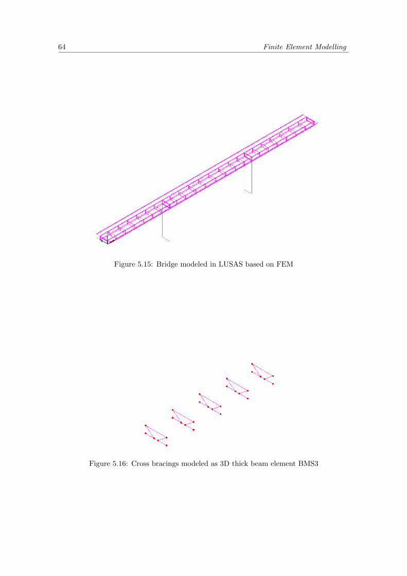
64 Finite Element Modelling
Figure 5.15: Bridge modeled in LUSAS based on FEM
Figure 5.16: Cross bracings modeled as 3D thick beam element BMS3

LUSAS FEM 65
Shell elements
The surfaces are designed as 3D thin shell elements QSI4. These elements take intoaccount both membrane and flexural deformations and the transverse shear defor-mations are not included. The directional material properties are defined in thelocal axes of the elements. The elements are assigned as isotropic in nature and themass is modeled as lumped mass. The membrane stresses vary in a linear mannerin QSI4 elements and all the loads applied on the membranes are lumped at thenodes. These elements cannot be used for non-linear behavior of materials. Thedeck surface, the I-girders and the stiffeners are modeled as QSI4 shell elements.The thicknesses are assigned as per the drawings. The piers are also modeled asthin shell elements and then the thickness is assigned. The following figure providesa description of the thin shell elements in the bridge model.
Figure 5.17: Shell elements represented by the surfaces marked in ‘green’
Mesh
A regular mesh of element size 0.5 has been used for both lines and surfaces. Thecross bracings are modeled as line elements and the remaining structural membersare modeled as surface elements. The mesh size of 0.5 was chosen as it provided theappropriate density of the mesh which generated practically accurate results andalso the computer processing time was within limits.

66 Finite Element Modelling
Figure 5.18: Mesh of bridge components
Loading
The bridge model was assigned its self-weight by the option of ‘Body Force’ inLUSAS. The acceleration due to gravity value was assigned as 9.81 m/s2.
Figure 5.19: Self-weight acting on the deck surface
5.1.7 Analysis of different boundary conditions
During the modeling of a structure for performing a finite element analysis, theboundary conditions have quite a significant impact on the results obtained. Suit-able assumptions regarding the support conditions and boundary restrains are nec-essary for the accurate analysis and estimation of results for a structure in a givenload case scenario.
For the problem under consideration in this report, various possible outcomes anddiscrepancies have been observed by editing the boundary conditions. The possiblecases that were modeled and analyzed in this report are mentioned as follows:

LUSAS FEM 67
• Modeling the foundation of the bridge piers with spring stiffness values takingthe soil-structure interaction into account and the abutments as being simplysupported with hinge and roller supports as shown in the figure 5.20.
• Modeling the bridge with piers and the foundation slabs and assigning a springstiffness values to the foundation slabs so that they behave as flexible struc-tures. The abutments are modeled as simply supported as the previous caseshown in the figure 5.21.
Figure 5.20: Bridge modeled with spring supports without considering the footing
Figure 5.21: Bridge modeled with spring supports with considering the footing
• Modeling the bridge without the piers and the foundation slabs and assumingthe bridge to be simply supported at the abutments and at the intermedi-ate supports. One of the abutments is assigned as a hinge support and theremaining three supports are assigned as roller supports shown in the figure5.22:
The case consisting of the spring stiffness boundary condition at the pier supportsis further subdivided into two cases. The first case considers the spring stiffnessvalues for the soil-structure interaction computed and provided by Ramboll AB.The spring stiffness values provided for the supports 2 and 3 are shown in thetable 5.2 : In the second case, we have computed the spring stiffness values for a

68 Finite Element Modelling
Figure 5.22: Bridge modeled without considering piers
Table 5.2: Spring stiffness for supports 2 and 3, case1 (Ramboll value) and case 2 (Gazetas,1991)
Case 1 Case 2
Support 2 Support 3 Support 2 Support 3 Unit
1 Length of the footing 11 11 11 11 m2 Breadth of the footing 6.3 6.3 6.3 6.3 m3 E-value of soil 79 105 79 105 MPa4 Rotational stiffness kφ,x 6.898.106 9.168.106 15.62.106 20.76.106 kNm/rad5 Rotational stiffness kφ,x 12.04.106 16.01.106 35.15.106 46.71.106 kNm/rad
rectangular footing based on Literature (Gazetas, 1991) and the values are in table5.2:
The results obtained by the analysis are presented in details in the next chap-ter. For case 1, the fundamental frequencies were observed to be the lowest whenthe spring stiffness values provided by Ramboll were used. The first fundamentalfrequency was observed to be 0.724 Hz and it had a transversal fundamental modeshape. The second mode of vibration was vertical in shape. When the spring stiff-ness values from Gazetas, 1991 were used, the fundamental frequency increased asexpected from 0.724 Hz to 0.92 Hz due to higher spring stiffness values. The modeshapes were observed to be identical as the boundary conditions were not altered.
For case 2, when the foundation slabs of the bridge under the piers were consid-ered to behave in a flexible manner and are assigned with the spring stiffness values,the frequencies observed were higher than the previous observed cases. This obser-vation was obvious from the fact that the addition of the foundation slabs to thestructure will increase the total mass of the structure resulting in an increase of thestiffness of the bridge. In this case the spring stiffness values that were provided byRamboll were used for the analysis and the first fundamental frequency of the bridgewas observed to be 0.961 Hz. The fundamental mode shapes did not show any vari-ation with the first case and the first fundamental mode shape was transversal andthe second mode was vertical in shape.
For case 3, the bridge deck was modeled as a simply supported beam on one hinge

LUSAS FEM 69
and three roller supports. The model was analyzed for frequencies and mode shapesand the first fundamental frequency was observed to be 1.578 Hz. The first funda-mental mode shape was vertical in nature and the second fundamental mode shapewas transversal in nature. The results for the frequencies and mode shapes obtainedwere found to be exactly similar to the case if the bridge was modeled with a foun-dation slab and a fixed boundary condition was assigned to the foundation.
After a complete understanding of the behavior of the bridge under varying bound-ary conditions and restrains, we decided to proceed with our calculations based onthe most critical case. From the results it is quite evident that the most critical caseis the first case with the spring stiffness values provided by Ramboll. This case hadthe lowest fundamental frequency of all the cases and had a transversal first modeshape of vibration. When a structure has a lower fundamental frequency then it ismore prone to dynamic behavior being imposed by wind action. Lower frequencyindicates a lower stiffness and signifies that the structure can be easily excited tovibrate in its first mode by a low frequency harmonic load. This means that a lowerwind velocity can induce large amplitude of vibrations on the structure if the fre-quency of the induced load is in the range of one of the natural frequencies of thestructure resulting in resonance.
The participation factors and the sum mass participation factors were also gener-ated from LUSAS for all the above discussed cases. A detailed report of the resultsincluding the mode shapes, Eigen values and Eigen frequencies, sum mass participa-tion and the participation factors have been presented and discussed in Chapter 6.The sum mass participation factor provides a platform to identify the most signifi-cant modes that need to be analyzed and it generally provides a cut-off boundaryof 90

70 Finite Element Modelling
5.2 MATLAB FEM
The bridge is also modeled as a 2-dimensional finite element structure and analyzedin MatLab to generate the fundamental frequencies and mode shapes. The bridgeelements are designed as Beam Element (Euler-Bernoulli Beam) where the sheardeformations are not taken into account. The elemental stiffness matrix of theEuler-Bernoulli beam along with the transformation matrix is shown as follows:
A general representation of the degrees of freedom of an Euler-Bernoulli beam isthe following figure:
Figure 5.23: Degrees of freedom in 2D beam element
In MatLab, the degrees of freedom of the structure have been specified at eachnode. The bridge deck is sub-divided into 23 members by various nodes and thepiers are sub-divided into three members each.
Figure 5.24: Degrees of freedom of the structural elements
Each node has three degrees of freedom, namely, translation along the x-direction,translation along the y-direction and rotation along the axis perpendicular to theplane of the paper. Hence, it is clearly visible from the diagram that the degrees of

MATLAB FEM 71
freedom of the bridge are numbered from 1 to 90 for all the 30 nodes i.e. 3 degreesof freedom for each node.
The boundary conditions that are assigned to the model are similar to thoseassigned in LUSAS for case 3. The left abutment (node 1) has been modeled as ahinge support with the translations (DOFs 1 and 2) in the x and y-directions asconstrained and the rotation (DOF 3) about the perpendicular axis as free. Theright abutment (node 24) has been modeled as a roller support with the translationin the y-direction (DOF 71) as constrained and the translation in the x-direction(DOF 70) and the rotation about the perpendicular axis as free (DOF 72). Thebases of the piers (node 27 and node 30) are assigned as fixed supports with boththe translations (DOFs 79, 80, 88 and 89) and the rotations (DOFs 81 and 90) tobe fixed and restrained.
The MatLab program generates the fundamental frequencies and the first threemodes shapes of the 2-dimensional structure. The detailed description of the MatLabprogram has been shown in Appendix B. The fundamental frequency value of the2-D bridge obtained from MatLab was found to be 1.476 Hz and the first threefundamental mode shapes are illustrated as follows:
Figure 5.25: Mode shapes obtained from MATLAB
The fundamental frequency value of 1.476 Hz is quite similar to that obtainedfrom LUSAS modeling the bridge as a simply supported bridge or with fixed foun-dation slabs. This shows that the modeling of the bridge in LUSAS is justified andaccurate and hence can be used for further extraction of results.


Chapter 6
Analysis and Results
In this chapter the total wind load acting over the bridge components is calculatedas it causes a wind-induced vibration over the bridge structure. The bridge has alength of 166m and three spans which is supported by two intermediate piers withequal distance of 50m away from abatements. The piers have a height of 23m fromthe footing levels. The dimension of the bridge is described in details in chapter5. The wind load and the corresponding bridge response is calculated by assumingthe deck as a continuous beam of three spans. The procedure is based on theconsideration that the deck is a line like structure. This is due to the fact thatthe vertical dimension of the deck is not in the same order of magnitude with thecharacteristic eddy sizes or the wave length taken at the natural frequency, (U/n).Also, the lack of correlation along the deck height does not significantly contributeto the response calculations. If, it is found that the width of the structure is equalor larger than the wave length taken at the natural frequency then the deck has tobe analyzed based on the ‘plate-line’ structures.
6.1 Natural frequencies and Mode shapes
6.1.1 Results from LUSAS
The natural frequencies of the bridge are obtained using finite element model,LUSAS and the results are then verified by MATLAB. The results which are ob-tained by MATLAB are very close to the values extracted from LUSAS. The bridgeis modeled by assuming two different boundary conditions; the fixed boundary con-dition and the spring boundary conditions. The values corresponding to the stiffnessof the spring are supplied by Ramboll (case 1) and used in analysis. However, thesprings stiffness may also be determined based on the modulus of the soil beneaththe footings for a rectangular footing based on Literature (Gazetas, 1991) (i.e. case2). The results are presented in table 5.2.
72

Natural frequencies and Mode shapes 73
Spring boundary condition
The first case is analyzed by modeling the bridge piers with spring support con-ditions. This case is further subdivided into two corresponding cases; case 1 forthe spring stiffness values provided by Ramboll and case 2 for the spring stiffnessvalues obtained from literature (Gazetas, 1991). The values of the spring stiffnessare provided in Table 5.2 for the respective intermediate piers.
The spring stiffness values obtained from literature (Gazetas, 1991) are higher thanthose provided by Ramboll. Hence, the eigen frequencies obtained for case 1 arelower than eigen frequencies obtained for case 2. Both the cases generate fundamen-tal mode shapes which are identical in nature. As case 1 gives lower fundamentalfrequencies, it is considered to be the more critical case of the two and further anal-ysis is performed for case 1.
The fundamental frequency for case 1 is obtained as 0.724 Hz and the correspond-ing mode shape is transversal in nature (Figure 6.1). The first fundamental modeis in the along-wind direction and the second mode of vibration is in the cross-winddirection having a frequency of 1.484 Hz. The mass participation along the y-axisis 75.82% for the first mode which signifies a considerable mass contribution of thetotal mass (Figure 6.4). The mass participations along the x and z-directions areconsiderably negligible for the first mode (Figure 6.3 and 6.5).
Fixed boundary condition
In this model, the bridge piers were assigned fixed boundary conditions and thetranslations and rotations about the x, y and z-directions were restricted. Theabutments were assigned similar boundary conditions as the previous case as hingeand roller supports. The fundamental frequencies and mode shapes were extractedfrom LUSAS and were compared and analyzed.
The first fundamental frequency for this case was obtained as 1.491 Hz and themode shape was a sinusoidal vertical deflection mode in nature (Figure 6.6). Thismode resembled the second mode shape of the previous case with spring supports.The fundamental frequency was observed to be higher than the previous case as thefixed boundary conditions imparted a rigid nature to the bridge. The mass partic-ipation along the x-direction was 1.54% which was higher than those along the yand z-directions (Figure 6.8, 6.9 and 6.10). The third mode of vibration showed asignificant mass participation of 66.38% along the y-direction as well (Figure 6.9).The sum mass participation for the first 50 modes was extracted and it was observedto reach 87% in the x-direction which can be approximated to 90%.
Piers
The piers were also analyzed and the eigen frequencies and mode shapes were ex-tracted from LUSAS. The piers were modeled independently with spring stiffnessvalues assigned to the base of the piers. The spring stiffness values used for this

74 Analysis and Results
Fixed boundary condition The mode shapes and mass participation is shown below.
Mode 1
F1 = 0.7235 Hz
Mode 2
F2 = 1.4848 Hz
Mode 3
F3 = 1.7869 Hz
Mode 4
F4 = 2.2121 Hz
Mode 5
F5 = 2.2765 Hz
Mode 6
F6 = 2.6301 Hz
Mode 7
F7 = 2.6332 Hz
Mode 8
F8 = 3.1753 Hz
Mode 9
F9 = 4.1435 Hz
Mode 10
F10 = 4.9304 Hz
Figure 6.1: Mode shapes and fundamental frequencies for the bridge with spring supports

Natural frequencies and Mode shapes 75
Figure 6.2: Modes and frequencies for spring support case
Figure 6.3: Percentage mass participation in x-direction for spring support case

76 Analysis and Results
Figure 6.4: Percentage mass participation in y-direction for spring support case
Figure 6.5: Percentage mass participation in z-direction for spring support case

Natural frequencies and Mode shapes 77
Mass participation ans natural frequencies:
Mode 2
F2 = 1,8026 Hz
Mode 1
F1 = 1,491 Hz
Mode 3
F3 = 2,064 Hz
Mode 4
F4 = 2,242 Hz
Mode 5
F5 = 2,617 Hz
Mode 6
F6 = 2,647 Hz
Mode 7
F7 = 3,033 Hz
Mode 8
F8 = 3,484 Hz
Mode 9
F9 = 4,396 Hz
Mode 10
F10 = 4,952 Hz
Figure 6.6: Mode shapes and fundamental frequencies for the bridge with fixed supports

78 Analysis and Results
Figure 6.7: Modes and frequencies for fixed support case
Figure 6.8: Percentage mass participation in x-direction for fixed support case

Natural frequencies and Mode shapes 79
Figure 6.9: Percentage mass participation in y-direction for fixed support case
Figure 6.10: Percentage mass participation in z-direction for fixed support case

80 Analysis and Results
case were those provided by Ramboll. The first fundamental frequency of the pierwas observed to be 1.363 HZ and it had a mode of vibration along the y-direction(Figure 6.11). The second modal frequency was observed to be 3.399 Hz and themode of vibration was along the x-direction. The first three modal frequencies andmode shapes for the two corresponding directions x and y were extracted to analyzethe pier for different directions of wind actions. Mode 1 showed a significant massparticipation of 66.92% along the y-direction which is obvious from the first modeof vibration (Figure 6.13). The second mode of vibration shows significant massparticipation of 63.97% along the x-direction which is justified by the second modeof vibration (Figure 6.15).
The first two modes of vibration are analyzed further in this chapter for wind actionsalong the y and x-directions respectively.
Table 6.1: Frequencies, percentage mass participation and percentage sum mass partici-pation for deformation along y-axis
Frequency (Hz) (%) Mass Participation (%) Sum Mass Participation
Mode 1 1.362 66.92 66.92Mode 4 9.287 18.25 85.17Mode 8 27.137 5.52 90.69
Table 6.2: Frequencies, percentage mass participation and percentage sum mass partici-pation for deformation along x-axis
Frequency (Hz) (%) Mass Participation (%) Sum Mass Participation
Mode 2 3.399 63.97 63.97Mode 7 20.495 19.04 83.01Mode 12 52.458 7.01 90.02
6.1.2 Results from Matlab
A 2-dimensional model similar to the actual bridge was analyzed in MATLAB andthe fundamental frequencies and mode shapes were extracted. The modes of vibra-tions are along the vertical direction (Figure 6.16). The fundamental frequency was1.467 Hz and the first ten fundamental frequencies were extracted (Table 6.3).
The results obtained from MATLAB comply with those which are obtained fromLUSAS for the fixed boundary condition case (Table 6.3). This shows that themodeling in LUSAS is justified and hence will provide satisfactory results for modalfrequencies and mode shapes.
6.2 Power spectral density function
There are four different Power Spectral Density Functions which can be found inliterature for analyzing the wind action on structures (Chapter 2.4.3 Figure 2.4).

Power spectral density function 81
Mode 1
F1 = 1,363 Hz
Mode 2
F2= 3,399 Hz
Mode 3
F3= 6,679 Hz
Mode 4
F4= 9,287 Hz
Mode 5
F5 = 17,950 Hz
Mode 6
F6= 19,996 Hz
Mode 7
F7= 20,495 Hz
Mode 8
F8= 27,137 Hz
Mode 9
F9=33,339 Hz
Mode 10
F10=35,737 Hz
Mode 11
F11= 46,955 Hz
Mode 12
F12= 52,458 Hz
Figure 6.11: Mode shapes and frequencies of piers

82 Analysis and Results
Figure 6.12: Modes and frequencies of piers for deformations along y-axis
Figure 6.13: Percentage mas participation of piers for deformations along y-axis

Power spectral density function 83
Figure 6.14: Modes and frequencies of piers for deformations along x-axis
Figure 6.15: Percentage mas participation of piers for deformations along x-axis

84 Analysis and Results
Table 6.3: Comparison between the frequencies obtained from MATLAB with the fre-quencies along z-axis in LUSAS
MATLAB LUSAS
Mode Frequency(Hz) Mode Frequency (Hz)
1 1.467 1 1.4912 1.742 4 2.2423 1.867 6 2.6474 3.611 9 4.3975 4.685 11 5.0776 5.683 14 6.9397 5.905 15 7.2328 7.973 16 7.4299 9.100 18 7.91210 11.060 21 9.118
Among these, the two most commonly used PSDF are von Karman spectral densityand Kaimal spectral density which is shown in the figure 2.5. Eurocode 1 is basedon the Kaimal spectral density function (Equation 2.26) and Swedish Annex SS-EN-1-4-2005 is based on the von Karman spectral density function (Equation 2.27).Hence, in this report we have analyzed the wind response based on the von Karmanspectral density function.
Eurocode 1 suggests the value of integral length scale Lxu to be 180 m and theSwedish annex suggests a value of Lxu to be 150 m. In this report, we have analyzedthe spectral response based on an integral length scale of 150 m (Figure 2.5). Fromthe mentioned figure, it is clear that for a non-dimensional frequency fL of 0.04, thevon Karman spectral density gives a higher response value than the Kaimal spectraldensity and for a non-dimensional frequency fL of 0.6, the Kaimal spectral densitygives a higher response value than the von Karman spectral density.
6.2.1 Deck
In the analysis of the bridge deck against wind action, the two cases for springsupport condition and fixed support condition are analyzed independently. For thecase with spring support, the first two modes generate a non-dimensional frequencyvalue which seems to be within the range of spectral density function (Figure 6.17).These two cases are first analyzed separately and then together and the gust factorsfor both the cases are calculated which is shown further in the chapter. For the casewith fixed boundary conditions, the only the first fundamental mode of vibration isanalyzed as this generates a non-dimensional frequency fL which is in range of thespectral density function. This value of fL is similar to that generated by the secondmodal vibration of the previous case (Figure 6.17). The non-dimensional frequencyfL for the corresponding vibration modes is calculated according to Equation 2.25.

Power spectral density function 85
Figure 6.16: Mode shapes obtained from MATLAB
Figure 6.17: Power spectral density function of the deck(von Karman)

86 Analysis and Results
6.2.2 Piers
For the case of piers, the analysis is performed for two different wind directions,namely x and y-direction. The modes and frequencies along these directions areextracted and the corresponding non-dimensional frequencies are calculated. It isfound out that only the first fundamental mode of vibration (f1 = 1.362Hz) providesa non-dimensional frequency fL which falls within the range of the spectral densityfunction (Figure 6.18). This mode of vibration is along the y-direction and the gustfactor and other dynamic analysis parameters are calculated further in this chapter.
Figure 6.18: Power spectral density function of the pier (von Karman)
6.3 Response-influence function
6.3.1 Deck
In order to calculate the dynamic response of the structure the influence responsefunction of the structure is required. The response may be in the form of bendingmoment, deflection or stress. For this case i.e. continuous beam with three spans,the normalized bending moment influence line diagram for the central mid-span isshown in figure 6.19. The bending moment influence function is normalized withrespect to the maximum bending moment value at the central mid-span i.e IR,ref .The IR,ref is the maximum response which here is equal to 11.55.
6.3.2 Piers
The response influence functions (IR) of the piers are assumed to have a constantsign. The corresponding response influence functions for such structures are shown

Wind Load Analysis 87
Figure 6.19: Bending moment influence function for the three continuous span beam
in Table 3.1. The entire procedure to calculate IR is given in the section 3.1.2.
6.4 Wind Load Analysis
The structure has a main span of the 66m which is higher than the 50m. Thereforea dynamic assessment of the bridge is needed based on the Swedish annex. Addi-tionally the two first natural freguencies are falling within the range of the powerspectral density functions. In this section, first the corresponding gust factor isobtained and then the maximum wind load acting over the structure is determined.
6.4.1 Determination of Gust factor
The wind analysis of the structure is performed based on three cases mentioned asfollows:
• Bridge with intermediate piers having spring boundary conditions.
• Bridge with intermediate piers having fixed boundary conditions.
• Piers
Bridge with intermediate piers having spring boundary conditions
This case is subdivided into two cases. In the first case, only the first mode of vi-bration is considered to be the governing mode of vibration and hence the analysisis performed considering only the first fundamental frequency. For the second case,both the first and the second modes of vibrations are considered to be the governing

88 Analysis and Results
modes of vibrations and hence the response of the structure to the wind action isanalyzed for both the modes.
Table 6.4 provides the input parameters required for the analysis and calculation ofgust factor. Table 6.5 shows the calculation of gust factor for the case consideringonly the first fundamental mode as the governing mode of vibration. Table 6.6 showsthe calculation of the gust factor for the case considering the first two fundamentalmodes of vibrations together as the governing modes.
Table 6.4: Input parameters
spring fixed
support support Unit Comment
Wind climate1 Reference wind velocity Ubas 23 23 m/s SS-EN-Table NA1
2 Air density ρ 1.25 1.25 kg/m3
Site specifications3 Roughness length z0 0.05 0.05 m SS-EN-Table 4.1
4 Terrain factor 0.19 0.19Structural specifications
5 Horizontal dimension b 166 166 m6 Vertical dimension h 3.5 3.5 m7 Natural frequency ne 0.742 1.48 Hz FEM (LUSAS)
8 Logarithmic decrement δs 0.04 0.04 SS-EN-Table F.2
9 Mass per unit of length 10843.37 10843.37 kg/m10 Mass per unit of area µ 3098.1 3098.1 kg/m2
11 Shape factor C 1.56 1.56 SS-EN-Figure 8.3
Bridge with intermediate piers having fixed boundary conditions
For this case, the support condition for the intermediate piers is assigned as fixedand the bridge deck is analyzed for the along-wind response. For this case, it hasbeen shown previously from the Power Spectral Density Function that only thefirst mode generates a non-dimensional frequency which has a significant response.Hence, only the first fundamental mode is considered to be the governing mode andthe gust factor is calculated based on the first fundamental frequency as shown inTable 6.5.
Piers
For the case of the piers, it has been shown previously in this chapter that onlythe first fundamental mode of vibration along the y-direction generates a non-dimensional frequency which shows a significant response in the Power SpectralDensity (PSDF) diagram. The second mode of vibration generates a response whichfalls out of the range of the PSDF diagram. Hence, the dynamic wind analysis ofthe piers is performed for the first fundamental mode of vibration and the details ofthe calculation are shown in Table 6.7 and Table 6.8.

Wind Load Analysis 89
Table 6.5: Design parameters of the bridge deck
spring fixed
support support Unit Comment
1 Reference height zref 25 25 m2 Mean wind velocity U(zref ) 27.16 27.16 m/s Eq. 3.563 Reference Influence number 11.55 11.55 Nm/N Figure 3.14 Integral effect of gm i.e. γm 0.105 0.105 Eq. 3.435 Mean bending moment at mid-span 506.7 506.7 kN/m Eq. 3.426 Turbulence intensity Iu(zref ) = Iu,ref 0.161 0.161 Eq. 2.147 Integral length scale Lu = Lxu(zref ) 131.64 131.64 m Eq. 3.578 Lyu = Lu/3 43.88 43.88 m9 Non-dimensional response variance J2
b 0.021 0.021 Eq.3.4710 Background bending moment σb 32.61 32.61 kN/m Eq. 3.4611 Aero-dynamic damping δa 0.0113 0.0055 Eq. 3.6612 Total damping δ 0.0513 0.00.0455 Eq. 3.6513 Non-dimensional frequency fL 3.51 7.17 Eq. 2.2514 Spectral density function RN (zref , ne) 0.0497 0.0308 Eq. 2.2715 φy = Cynb/Uref (Cy = 8) 35.403 72.3716 Joint acceptance function Jy(ne)
2 0.02804 0.0136 Eq. 3.5117 Equivalent mass mg 9.105 9.105 kg Eq. 3.3918 Variance of acceleration σacc 0.0544 0.0318 m Eq. 3.5319 Resonant bending moment σr 194.57 94.53 kNm Eq. 3.5320 Peak factor Kp(v = ne) 3.651 3.841 Eq. 3.5921 Standard deviation of 197.28 99.998 kNm Eq. 3.26
Structural response σR22 Maximum bending moment Rmax 1226.97 890.83 kNm Eq. 3.2523 Gust factor ϕ = Rmax/µR 2.421 1.758 Eq. 3.25
6.4.2 Determination of Maximum Wind Load on the Structure
The maximum wind load calculations for the bridge deck are shown in table 6.9 forthe three cases mentioned previously, i.e. spring support condition with first modeas the governing mode, spring support condition with the first two modes as thegoverning modes and fixed support condition with the first fundamental mode asthe governing mode of vibration.
Table 6.10 also shows three different load conditions, i.e. without traffic, with trafficand under construction. In the case of without traffic, the vertical dimension ofthe deck is equal to 4 m and for the case of with traffic, the vertical dimension ofthe deck is 6 m taking into consideration the height of the vehicles. In the caseof under construction, it is assumed that the two girders are placed over the piersbefore installing the concrete deck. Therefore, the vertical dimensions of the twogirders are calculated to be 5.1 m taking into consideration the effect of both thegirders. The basic wind velocity vb during the construction is taken as 15 m/s.The corresponding maximum wind loads per unit length of the deck in x-direction(along-wind direction) are shown in table 6.11. The maximum wind in the vertical

90 Analysis and Results
direction i.e. z-direction is taken as the same as that of in x-direction but the forcecoefficient cfz is taken as ±0.9 which is recommended by EC1 (cl. 8.3.3) . Themaximum wind force in y-direction is taken as 25% of the force in x-direction forplated bridges based on cl. 8.3.4 of EC1.
For the piers, table 6.12 shows the maximum wind load per unit length actingon the pier based on the gust factor calculated in table 6.9.
6.5 Vortex shedding and Aeroelastic instabilities
6.5.1 Vortex shedding
For the bridge deck, the ratio between the critical vortex shedding velocity and themean wind velocity is calculated to be 1,404. Annex E.1.2(2) specifies that the vor-tex shedding response need not be checked if the above ratio exceeds 1,25. Hence,it can be concluded that the bridge deck will be safe against vortex shedding insta-bility.
The maximum deflection caused due to the vortex shedding load on the piers iscalculated to be 0,036m which is quite negligible when compared to the total heightand the cross-sectional dimensions of the pier. Hence, it can be concluded that thepiers will not be affected by vortex shedding and the resultant deflections are withinsafe limits. The detailed calculations are shown in the Appendix.
6.5.2 Galloping
Eurocode1 mentions that for a structure to be declared safe against galloping in-stability, the ratio between the onset galloping velocity and the mean wind velocityshould be greater than 1,25. In our case, the above ratio is 2,259 and hence it canbe concluded that the bridge deck is safe against galloping instability.
6.5.3 Divergence and Flutter Response of the Bridge Deck
The divergence and flutter response of the bridge deck is analyzed with the help ofEN1991-1-4 Annex E.4. Divergence and flutter are aerodynamic instabilities thatcan occur for plate-like structures above a certain threshold or critical wind veloc-ity. To avoid divergence and flutter, three criteria are given in EC1 to check thesusceptibility of a structure to these instabilities. The three criteria are checked inorder stated and if any one of the criteria is not met, then the structure will not beprone to either divergence or flutter.
The three criteria provided by EC1 are as follows:
• The structure or a substantial part of it has an elongated cross-section similarto a flat plate with b/d less than 0.25.

Vortex shedding and Aeroelastic instabilities 91
Hence, b/d = 3.5/12.01 = 0.291 which is greater than 0.25. Thus, the firstcriterion is not met and so the bridge deck will not be prone to either divergenceor flutter. The remaining two criteria that are mentioned below need not befurther checked:
• The torsional axis is parallel to the plane of the plate and normal to the winddirection. The center of torsion is at least d/4 downwind of the windward edgeof the plate.
• The lowest natural frequency corresponds to a torsional mode, or else thelowest torsional natural frequency is less than 2 times the lowest translationalnatural frequency.

92 Analysis and Results
Table 6.6: Determining the gust factor by considering the effect of first two mode shapesfor spring support.
Mode 1 Mode 2
Wind climate1 Reference wind velocity Ubas 23 23 m/s SS-EN-Table NA1
2 Air density ρ 1.25 1.25 kg/m3
Site specifications3 Roughness length z0 0.05 0.05 m SS-EN-Table 4.1
4 Terrain factor 0.19 0.19Structural specifications
5 Horizontal dimension b 166 166 m6 Vertical dimension h 3.5 3.5 m7 Natural frequency ne 0.742 1.48 Hz FEM (LUSAS)
8 Logarithmic decrement δs 0.04 0.04 SS-EN-Table F.2
9 Mass per unit of length 10843.37 10843.37 kg/m10 Mass per unit of area µ 3098.1 3098.1 kg/m2
11 Shape factor C 1.56 1.56 SS-EN-Figure 8.3
12 Reference height zref 25 25 m13 Mean wind velocity U(zref ) 27.16 27.16 m/s Eq. 3.5614 Reference Influence number 11.55 11.55 Nm/N Figure 3.115 Integral effect of gm i.e. γm 0.105 0.105 Eq. 3.4316 Mean bending moment at mid-span 506.7 506.7 kN/m Eq. 3.4217 Turbulence intensity Iu(zref ) = Iu,ref 0.161 0.161 Eq. 2.1418 Integral length scale Lu = Lxu(zref ) 131.64 131.64 m Eq. 3.5719 Lyu = Lu/3 43.88 43.88 m20 Non-dimensional response variance J2
b 0.021 0.021 Eq.3.4721 Background bending moment σb 32.61 32.61 kN/m Eq. 3.4622 Aero-dynamic damping δa 0.0113 0.0055 Eq. 3.6623 Total damping δ 0.0513 0.00.0455 Eq. 3.6524 Non-dimensional frequency fL 3.51 7.17 Eq. 2.2525 Spectral density function RN (zref , ne) 0.0497 0.0308 Eq. 2.2726 φy = Cynb/Uref (Cy = 8) 35.403 72.3727 Joint acceptance function Jy(ne)
2 0.02804 0.0136 Eq. 3.5128 Equivalent mass mg 9.105 9.105 kg Eq. 3.3929 Variance of acceleration σacc 0.0544 0.0318 m Eq. 3.5330 Resonant bending moment σr 194.57 94.53 kNm Eq. 3.5331 Peak factor Kp(v = ne) 3.651 3.841 Eq. 3.5932 Standard deviation of 197.28 99.998 kNm Eq. 3.26
Structural response σR32 Total resonant response σR 221.18 kNm Eq. 3.2433 Maximum bending moment Rmax 1356.34 kNm Eq. 3.2534 Gust factor ϕ = Rmax/µR 2.677 Eq. 3.25
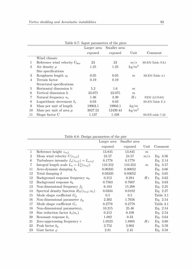
Vortex shedding and Aeroelastic instabilities 93
Table 6.7: Input parameters of the piers
Larger area Smaller area
exposed exposed Unit Comment
Wind climate1 Reference wind velocity Ubas 23 23 m/s SS-EN-Table NA1
2 Air density ρ 1.25 1.25 kg/m3
Site specifications3 Roughness length z0 0.05 0.05 m SS-EN-Table 4.1
4 Terrain factor 0.19 0.19Structural specifications
5 Horizontal dimension b 5.2 1.6 m6 Vertical dimension h 23.075 23.075 m7 Natural frequency ne 1.36 3.39 Hz FEM (LUSAS)
8 Logarithmic decrement δs 0.03 0.03 SS-EN-Table F.2
9 Mass per unit of length 19903.1 19903.1 kg/m10 Mass per unit of area µ 3827.52 12439.44 kg/m2
11 Shape factor C 1.137 1.428 SS-EN-table 7.23
Table 6.8: Design parameters of the pier
Larger area Smaller area
exposed exposed Unit Comment
1 Reference height zref 13.845 13.845 m2 Mean wind velocity U(zref ) 24.57 24.57 m/s Eq. 3.566 Turbulence intensity Iu(zref ) = Iu,ref 0.1778 0.1778 Eq. 2.147 Integral length scale Lu = Lxu(zref ) 110.252 110.252 m Eq. 3.5711 Aero-dynamic damping δa 0.00335 0.00052 Eq. 3.6612 Total damping δ 0.03335 0.03052 Eq. 3.6512 Background response frequency n0 0.212 0.284 Hz Eq. 3.6212 Background response kb 0.7563 0.7607 Eq. 3.6313 Non-dimensional frequency fL 6.104 15.208 Eq. 2.2514 Spectral density function RN (zref , ne) 0.0334 0.0182 Eq. 2.2715 Mode shape coefficient Gy 0.5 0.5 Table 3.116 Non-dimensional parameter φy 2.302 1.7656 Eq. 2.5417 Mode shape coefficient Gz 0.2778 0.2778 Table 3.118 Non-dimensional parameterφz 10.215 25.46 Eq. 2.5419 Size reduction factor ks(ne) 0.212 0.109 Eq. 2.5420 Resonant response kr 1.082 0.33 Eq. 3.6421 Zero-uppcrossing frequency v 1.0523 1.8805 Hz Eq. 3.6022 Peak factor kp 3.752 3.903 Eq. 3.5923 Gust factor ϕ 2.81 2.45 Eq. 3.58

94 Analysis and Results
Table 6.9: Design parameters of the piers obtained from Eurocode1
Larger area Smaller area
exposed exposed Unit Comment
Wind climate1 Reference wind velocity Ubas 23 23 m/s SS-EN-Table NA1
2 Air density ρ 1.25 1.25 kg/m3
Site specifications3 Roughness length z0 0.05 0.05 m SS-EN-Table 4.1
4 Terrain factor 0.19 0.19Structural specifications
5 Horizontal dimension b 5.2 1.6 m6 Vertical dimension h 23.075 23.075 m7 Natural frequency ne 1.36 3.39 Hz FEM (LUSAS)
8 Logarithmic decrement δs 0.03 0.03 SS-EN-Table F.2
9 Mass per unit of length 19903.1 19903.1 kg/m10 Mass per unit of area µ 3827.52 12439.44 kg/m2
11 Shape factor C 1.137 1.428 SS-EN-table 7.23
12 Reference height zref 13.845 13.845 m13 Mean wind velocity U(zref ) 26.808 26.808 m/s EC1,Eq. 4.3
14 Turbulence intensity Iu(zref ) = Iu,ref 0.161 0.161 Eq. 4.7
15 Integral length scale Lu = Lxu(zref ) 150 150 m16 Aero-dynamic damping δa 0.001 0.001 Table F.2
17 Total damping δ 0.031 0.03118 Background response factor B2 0.961 0.97 Swedish Annex
19 Non-dimensional frequency fL 7.01 18.968 Swedish Annex
20 Spectral density function RN (zref , ne) 0.03 0.01621 Non-dimensional parameter φb 0.542 0.60722 Non-dimensional parameterφh 0.299 0.14623 Resonant response Factor R2 0.977 0.29124 Zero-uppcrossing frequency v 0.965 1.628 Hz25 Peak factor kp 3.735 3.87226 Structural factor cscd 1.257 1.128 Cl. 6.3.1
27 Gust factor ϕ 2.674 2.399
Table 6.10: Input parameters to determine maximum wind load acting along the decklength
Without With During
traffic traffic construction unit Comment
vertical dimension dtot 4 6 5.278 mReference areaAref 664 996 876.148 m2
Force coefficient Cfx 1.56 1.87 1.65Basic wind velocity vbas 23 23 15 m/sAir Density 1.25 1.25 1.25 kg/m3

Vortex shedding and Aeroelastic instabilities 95
Table 6.11: Maximum wind load acting along the deck length
Spring support Spring support Fixed
(1st mode) (1st and 2nd modes) support unit Comment
Gust factor 2.422 2.678 1.758Air Density 1.25 1.25 1.25 kg/m3
Mean load Uz,ref (z) 27.16 27.16 17.71 m/s
Without Traffic 6.965 7.699 5.057 kN/m Eq. (2.37)(2.39)With traffic 12.524 13.844 9.093 kN/m Eq. (2.37)(2.39)Under Construction 4.134 4.57 3.002 kN/m Eq. (2.37)(2.39)
Table 6.12: Maximum wind load acting along the pier length
Larger area Smaller area
exposed exposed Unit Comment
Reference area 120 36.92 m2
Gust factor 2.81 2.45Shape factor 1.137 1.428Air Density 1.25 1.25 kg/m3
Mean load Uz,ref (z) 24.57 24.57 m/s
Maximum wind load 6.23 2.112 kN/m Eq. (2.37)(2.39)
Table 6.13: Vortex shedding response of bridge deck
Values Unit Comment
1 Fundamental frequency in crosswind direction f1 1.48 Hz2 Width of the deck in the crosswind direction d 3.5 m3 Width of the deck in the alongwind direction b 12.01 m4 Strouhal Number St 0.142 Fig. E.1 EC15 Density of air ρ 1.25 kg/m3
6 Structural logarithmic decrement of damping δs 0.047 Mass per unit length me 10843.37 kg/m8 Critical velocity for vortex shedding Ucrit 36.4788 m/s9 Mean wind velocity at the center 27.16 m/s
of the deck Um10 Ratio of critical velocity to 1.343
mean wind velocity (Ucrit/Um)11 Max. governing ratio for susceptibility 1.25 E.1.2(2) EC1
to vortex shedding (Ucrit/Um)1

96 Analysis and Results
Table 6.14: Vortex shedding response of piers
Values Unit Comment
1 Fundamental frequency in crosswind direction f1 1.362 Hz2 Width of the pier in the crosswind direction d 1.6 m3 Width of the pier in the alongwind direction b 5.2 m4 Strouhal Number St 0.107 Fig. E.1 EC15 Density of air ρ 1.25 kg/m3
6 Structural logarithmic decrement of damping δs 0.037 Height of the piers h 23.075 m8 Mass per unit length me 19903.1 kg/m9 Scruton Number Sc 373.183110 Assumed correlation length Lj 9.6 m11 Critical velocity for vortex shedding Ucrit 20.3664 m/s12 Mean wind velocity at the center 22.53 m/s
of the correlation length Um,Lj13 Basic value of standard deviation of load clat,0 1.1 Table E.2 EC114 Ratio of critical velocity to 0.9039
mean wind velocity (Ucrit/Um,Lj)15 Standard deviation of load clat 0.913516 Mode shape factor Kξ 0.13317 Effective correlation length factor Kw 0.80118 Maximum deflection amplitude ymax 0.0364 m
Table 6.15: Galloping response of bridge deck
Values Unit Comment
1 Fundamental frequency in crosswind direction f1 1.48 Hz2 Width of the deck in the crosswind direction d 3.5 m3 Width of the deck in the alongwind direction b 12.01 m4 Strouhal Number St 0.142 Fig. E.1 EC15 Density of air ρ 1.25 kg/m3
6 Structural logarithmic decrement of damping δs 0.047 Mass per unit length me 10843.37 kg/m8 Scruton Number Sc 56.659 Factor of galloping instability aG 1010 Onset velocity for galloping Ucg 58.69 m/s11 Mean wind velocity at the center 27.16 m/s
of the deck Um12 Ratio of onset velocity to 2.161
mean wind velocity (Ucg/Um)13 Max. governing ratio for susceptibility 1.25 E.2.1(2) EC1
to galloping (Ucg/Um)1


Chapter 7
Conclusion
EN-1991-1-4 or Eurocode 1, actions on structures-General Actions part 1-4, providescertain simplified methods that can be used as a guidance to determine the effectof fluctuating wind load on various types of structures and structural components.These methods are found to be based on a set of specific assumptions and simplifica-tions which restrict the applications of the code to structures having a complicatedresponse functions to the fluctuating wind load. If the wind-induced vibration ofthe structure is negligible i.e. the non-dimensional frequency of the structure isnot within the range of the power spectral density function (section 2.4.3), thenthe wind load is treated as a static wind load case and the simplified method sug-gested in clause 8.3.2 can be used. The structures whose non dimensional frequencyfalls within the range, a dynamic assessment needs to be performed. Eurocode1 presents specific methods to determine the structural factor which are applica-ble only for particular structural configurations (figure 6.1 EC1) whose response-influence functions have constant signs. The formula to obtain the aerodynamicadmittance functions that are presented in Eurocode 1 (annex B and C) are validfor structures whose response-influence functions have constant sign. For structureswhose response-influence function have complicated signs like the bending momentinfluence function of the given bridge in this report, these simplified methods maynot be appropriate to use in order to calculate the aerodynamic admittance function.
The other limitations behind the simplified methods to calculate the structuralfactors are that the along-wind vibration in the fundamental mode needs to besignificant and have a constant sign. This may not be valid for continuous bridgesfor which more than one mode shape may contribute to the response of the struc-ture against fluctuating wind load and one of the contributing fundamental modesmay vary in a complicated manner such as a sinusoidal function with changing sign.Hence, the aerodynamic admittance functions are obtained from multiple integralsof the normalized co-spectrum funtions and the mode shapes (section 3.1.2).
By comparing the results obtained from Eurocode1 and the analytical method pre-sented in chapter 3 for the piers which are analyzed as structural components havinga constant sign response-influence function and fundamental mode shape, it has beenobserved that the differences in the gust factor-values are very minor and both pro-
97

98 Conclusion
vide similar results. On the other hand, in the case of the three span bridge deck thebending moment influence function does not vary with a constant sign but rather ina complicated manner, the methods presented in Euocode 1 may not be appropriateto use and hence no comparison could be made between the results obtained fromthe theoretical methods and Eurocode 1.
The bridge is modeled using FEM with two separate boundary conditions, namelyspring support and fixed support conditions. It has been observed that modelingthe intermediate piers of the bridge as fixed supports increases the fundamental fre-quency of the structure and hence results in a lower value of the gust factor. Onthe other hand, modeling the footing of the intermediate piers as spring supportsreduces the fundamental frequency of the structure and changes the fundamentalmode shape which results in a higher value of the gust factor. It has also been ob-served that the resultant wind load acting on the structure increases by 13% whenthe dynamic response of the structure is considered.
From the above observations it may be concluded that one must be aware of the lim-itations and assumptions behind the simplified methods presented in the Eurocode1and knowledge of the concepts behind these suggested methods will enhance the ca-pability of a designer towards an efficient use of the given code. Further research isrecommended to analyse the deck of the bridge as a plate-like structure to evaluatethe dynamic response of the deck in two directions. A wind tunnel test if conducted,may also provide more accurate force coefficients for the bridge.

References
[1] Basu, R.I. (1983) ”Across-wind Response of Slender Structures of CircularCross-Section to Atmospheric Turbulence” PhD Thesis, BLWT-3-1983, Uni-versity of Western Ontario, London, Ontario, Canada.
[2] Bouassida, Y., Bouchon, E., Crespo, P., Croce, P., Davaine, L., Denton, S.,Feldmann, M.,Frank, R., Hanswille, G., Hensen, W., Kolias, B., Malakatas, N.,Mancini, G., Ortega, M., Raoul, J., Sedlacek, G., Tsionis, G. (2010) “BridgeDesign to Eurocodes Worked examples”. Bridge Design to Eurocodes, Vienna,4-6 October.
[3] Cook, N. (2007) “Designers’ Guide to EN 1991-1-4 Eurocode I: Actions onStructures, General Actions, Part 1-4: Wind Actions”. Designers’ Guide to theEurocodes.
[4] Davenport, A. G. (1961) ”The application of the statistical concepts to the windloading of the structures”. Proceeding of the Institution of Civil Engineers, 19,449-471.
[5] Davenport, A.G. (1962) “The response of slender line-like structures to a gustywind”. Proceedings of the Institution of Civil engineers, 23, 389-408.
[6] Davenport, A.G. (1967) “Gust loading factors”. Journal of the Structural divi-sion, ASCE, 93, 11-34.
[7] Davenport, A.G. (1977) “The prediction of the response of structures to gustywind”. Safety of Structures under Dynamic Loading, Hoalnd, Kavlie, Moe andSigbjornsson (eds.), Tapir, Trondheim, pp. 257-284.
[8] Davenport, A.G. (1982) “The reliability and synthesis of aerodynamic and me-teorological data for wind loading”. Seminar on Structural Aerodynamics, In-sititut Technique du Batiment et des Travaux Publics (ITBTP), St-Remy-Les-Chevreuse, France, April 20-22.
[9] Dyrbye, C. and Hansen, S.O. (1988) “Calculation for joint acceptance functionfor line-like structures”. Journal of Wind Engineering and Industrial Aerody-namics, 31, 210-430.
[10] Eurocode 1 (1995) “Basis of design and actions on structures-Part 2-4: Actionson structures-Wind actions”. European Prestandard ENV 1991-2-4.
99

100 References
[11] Eurocode 1 (2005) “Basis of design and actions on structures-Part 1-4: Actionson structures-Wind actions”. Svensk Standard SS-EN-1991-1-4:2005.
[12] Giosan, I.(2000) “Vortex shedding induced loads on free standing structures”.Structural Vortex Shedding Response Estimation Methodology and Finite Ele-ment Simulation, 1-20.
[13] Hansen, S.O. and Krenk, S. (1996) “Dynamic along-wind response of simplestructures”. Journal of Engineering, Mechanics ASCE.
[14] Harris, R.I.(1971) ”The nature of wind in the modern design of wind-sensitivestructures”. London: Construction Industry Research and Information Associ-ation.
[15] Isyumov, N. (2011) ”Announcement of the Alan G. Davenport Wind LoadingChain, Boundary Layer Wind Tunnel Laboratory”. The University of WesternOntario.
[16] Jain, A., Jones, N.P. and Scanlan, R.H. (1995) “Fully coupled buffeting analysisof long-span bridges”. Proceedings of the Ninth International Conference onWind Engineering, New Delhi, January, pp. 962-971.
[17] Kaimal, J.C., Wyngaard, J.C., Izumi, Y. and Cote, O.R. (1972) “Spectral char-acteristics of surface layer turbulence”. Journal of Royal Meteorological society,98, 563-589.
[18] Larsen, A. (1995) “Prediction for aeroelastic stability of suspension bridgesduring erection”. Proceedings of the Ninth International Conference on WindEngineering, New Delhi, January, pp. 917-927.
[19] Le, T.H., (2003) “Flutter aerodynamic stability analysis and some aerodynamiccontrol approaches of cable-stayed bridges (in Vietnamese)”. Master’s thesisat Vietnam National University of Hanoi.
[20] Morgenthal, G. (2000) “Fluid-Structure Interaction in Bluff-Body Aerodynam-ics and Long-Span Bridge Design: Phenomena and Methods”. PhD Thesis,CUED/D-STRUCT/TR.187, University of Cambridge.
[21] Sanpaolesi, L. and Croce, P. (2005) “ Handbook 4: Design of bridges: Guideto the basis of bridge design related to Eurocodes supplemented by practicalexamples”. Leonardo Da Vinci Pilot Project CZ/02/B/F/PP-134007.
[22] Scanlan, R. H. (1978) “The action of flexible bridges under wind. 2: Buffetingtheory J. ”. Sound and Vibration, 60(2), 201–211.
[23] Scanlan, R. H. (2000) “Bridge Deck Aeroelastic Admittance Revisited”. ASCE,J. Bridge Engineering, 5(1), pp. 1-7.
[24] Simiu, E. (1973) “Gust Factor and Alongwind Pressure Correlations”. Journalof Structural Division, 99, pp. 773-783.

References 101
[25] Simiu, E. (1974) “Wind Spectra and Dynamic Alongwind Response”. Journalof Structural Division, 100, pp. 1897-1910.
[26] Simiu, E. (1976) “Equivalent Static Wind Loads for Tall Building Design”.Journal of Structural Division, 102, pp. 719-737.
[27] Simiu, E. (1980) “Revised Procedure for Estimating Alongwind Response”.Journal of Structural Division, 106, pp. 1-10.
[28] Simiu, E. and Scanlan, R.H. (1986) Wind Effects on Structures. An Introductionto Wind Engineering. Second edition. Wiley, New York.
[29] Solari, G. (1982) “Design Wind Loads”. Proceedings of the 5th Colloquium onIndustrial Aerodynamics, Aachen, Germany. Part 2, pp. 73-86.
[30] Solari, G. (1982) “Alongwind Response Estimation: Closed Form Solution”.Journal of Structural Division, 108, 225-244.
[31] Theodorsen, Th. (1934) “General theory of aerodynamic instability and themechanism of flutter”. NACA Report No. 496, Washington DC.
[32] Trafikverkets foreskrifter om andring i Vagverkets foreskrifter (VVFS 2004:43)om tillampningen av europeiska berakningsstandarder (2011) “ TRVFS2011:12”. Trafikverkets forfattningssamling.
[33] TRVK Bro 11 (2011) “Trafikverkets tekniska krav Bro TRV publ nr 2011:085”.Trafikverket.
[34] Vickery, B.J. (1970) “On the reliability of gust loading factors”. Proceedingsof Technical Meeting concerning Wind Loads on Buildings and Structures, Na-tional Bureau of Standards, Washington, DC, 93-10.
[35] Vickery, B.J. and Basu, R.I. (1983) “Across-wind vibrations of structures ofcircular cross-section. Part 1. Development of a mathematical model for two-dimensional conditions”. Journal of Wind Engineering and Industrial Aerody-namics, 12, 49-73.
[36] von Karman, T. (1948) “Progress in the statistical theory of turbulence”, Jour-nal of Maritime Research, 7.

Appendices
102

Appendix A
Mass Participation Factor
Figure A.1: Modal analysis and mass participation factors of spring case
103
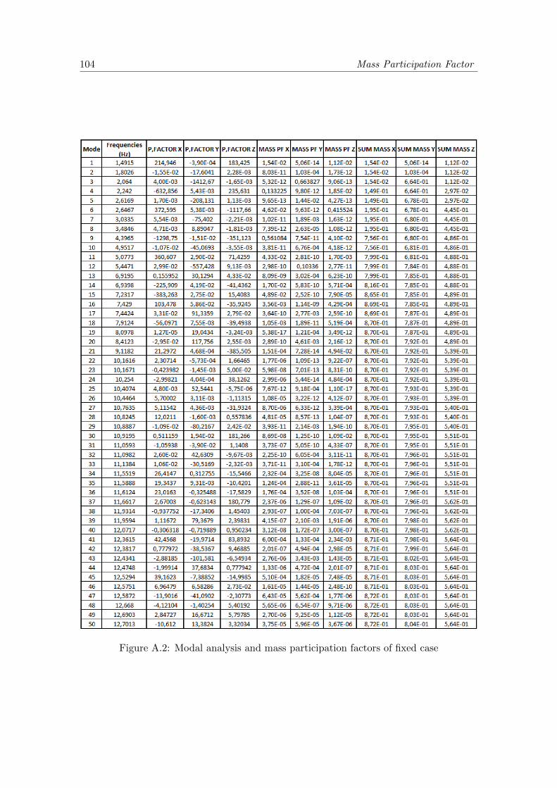
104 Mass Participation Factor
Figure A.2: Modal analysis and mass participation factors of fixed case

Appendices
105

Appendix B
MATLAB Code
106

%Determining the Natural frequencies and mode shapes of the given bridge %for fixed boundary conditions clc, clear all % section properties % span properties L_span= 166; Ls = L_span/23; %m A_span= 0.827 ; %m2 I_span =0.687 ; % m4 E_span= 6.868*10^10 ; %Pa EI_span= I_span*E_span ; m_el_span=1907000/23; % column properties A_clm= 1.5*6 ; %m2 I_clm =6*1.5^3/12; % m4 L_clm= 23/3 ; %m density= 2400 %kg/m3 E_clm= 33*10^9; %Pa EI_clm= I_clm*E_clm ; m_el_clm=density*A_clm*L_clm; % determinin the stiffness matrix and mass matrix element =[1 1 2 ; 2 2 3; 3 3 4 ; 4 4 5; 5 5 6; 6 6 7; 7 7 8; 8 8 9; 9 9 10; 10 10 11; 11 11 12; 12 12 13 ; 13 13 14; 14 14 15 ; 15 15 16; 16 16 17; 17 17 18; 18 18 19; 19 19 20; 20 20 21; 21 21 22; 22 22 23; 23 23 24; 24 8 25; 25 25 26; 26 26 27; 27 17 28; 28 28 29; 29 29 30];

edof= [ 1 1 2 3 4 5 6 ; 2 4 5 6 7 8 9; 3 7 8 9 10 11 12 ; 4 10 11 12 13 14 15; 5 13 14 15 16 17 18; 6 16 17 18 19 20 21; 7 19 20 21 22 23 24; 8 22 23 24 25 26 27; 9 25 26 27 28 29 30; 10 28 29 30 31 32 33; 11 31 32 33 34 35 36; 12 34 35 36 37 38 39; 13 37 38 39 40 41 42 ; 14 40 41 42 43 44 45; 15 43 44 45 46 47 48; 16 46 47 48 49 50 51; 17 49 50 51 52 53 54; 18 52 53 54 55 56 57; 19 55 56 57 58 59 60; 20 58 59 60 61 62 63; 21 61 62 63 64 65 66 ; 22 64 65 66 67 68 69; 23 67 68 69 70 71 72; 24 22 23 24 73 74 75; 25 73 74 75 76 77 78 ; 26 76 77 78 79 80 81; 27 49 50 51 82 83 84; 28 82 83 84 85 86 87; 29 85 86 87 88 89 90]; % span stiffness Matrix Kg1 = zeros(90); ne = 23; for i = 1:ne d1=Ls^2/12; k1 = A_span*E_span/Ls; k2= 12*EI_span/Ls^3; k3= 6*EI_span/Ls^2; k4= 4*EI_span/Ls; k5= 2*EI_span/Ls; kel_span = [ k1 0 0 -k1 0 0 0 k2 k3 0 -k2 k3 0 k3 k4 0 -k3 k5 -k1 0 0 k1 0 0 0 -k2 -k3 0 k2 -k3 0 k3 k5 0 -k3 k4]; m_el_s =eye(6,6); m_el_s(3,3)=d1; m_el_s(6,6)=d1; m_span= m_el_s * m_el_span/2; Kg1(edof(i,2:end),edof(i,2:end)) = Kg1(edof(i,2:end),edof(i,2:end)) + kel_span; end % column stiffness Matrix

Kg2 = zeros(90); ne = 29 for i = 24:ne Le_clm=3 %m d2=Le_clm^2/12 k1 = A_clm*E_clm/Le_clm; k2= 12*EI_clm/Le_clm^3; k3= 6*EI_clm/Le_clm^2; k4= 4*EI_clm/Le_clm; k5= 2*EI_clm/Le_clm; kel_clm = [ k1 0 0 -k1 0 0 0 k2 k3 0 -k2 k3 0 k3 k4 0 -k3 k5 -k1 0 0 k1 0 0 0 -k2 -k3 0 k2 -k3 0 k3 k5 0 -k3 k4] %transformation matrix T=[0 1 0 0 0 0 -1 0 0 0 0 0 0 0 1 0 0 0 0 0 0 0 1 0 0 0 0 -1 0 0 0 0 0 0 0 1] Kg_clm= T'*kel_clm* T; Kg2(edof(i,2:end),edof(i,2:end)) = Kg2(edof(i,2:end),edof(i,2:end)) + Kg_clm; end stiffness_matrix = Kg1+Kg2; K_total=Kg1+Kg2; % boundary conditions for stiffness matrix K_total(90,:)= []; K_total(:,90)= []; K_total(89,:)= []; K_total(:,89)= []; K_total(88,:)= []; K_total(:,88)= []; K_total(81,:)= []; K_total(:,81)= []; K_total(80,:)= []; K_total(:,80)= []; K_total(79,:)= []; K_total(:,79)= []; K_total(71,:)= []; K_total(:,71)= []; K_total(2,:)= []; K_total(:,2)= []; K_total(1,:)= []; K_total(:,1)= []; stiff_M =K_total;

% Mass Matrix % span mass Matrix Kg_mass_1= zeros(90); ne = 23; for i = 1:ne d1=Ls^2/12; m_el_s =eye(6,6); m_el_s(3,3)=d1; m_el_s(6,6)=d1; m_span= m_el_s * m_el_span/2; Kg_mass_1(edof(i,2:end),edof(i,2:end)) = Kg_mass_1(edof(i,2:end),edof(i,2:end)) + m_span; end % column mass Matrix Kg_mass_2= zeros(90); ne = 29 for i = 24:ne Le_clm=19,5/3 ;%m d2=Le_clm^2/12; %transformation matrix T=[0 1 0 0 0 0 -1 0 0 0 0 0 0 0 1 0 0 0 0 0 0 0 1 0 0 0 0 -1 0 0 0 0 0 0 0 1] Kg_clm= T'*kel_clm* T; %mass matrix column m_el_c =eye(6,6); m_el_c(3,3)=d2; m_el_c(6,6)=d2; m_column= m_el_c * m_el_clm/2; m_clm= T'*m_column* T; Kg2(edof(i,2:end),edof(i,2:end)) = Kg2(edof(i,2:end),edof(i,2:end)) + Kg_clm; Kg_mass_2(edof(i,2:end),edof(i,2:end)) = Kg_mass_2(edof(i,2:end),edof(i,2:end)) + m_clm; end mass_matrix =Kg_mass_1+ Kg_mass_2; M_total= Kg_mass_1+ Kg_mass_2; % boundary conditions for mass matrix M_total(90,:)= []; M_total(:,90)= []; M_total(89,:)= []; M_total(:,89)= []; M_total(88,:)= []; M_total(:,88)= []; M_total(81,:)= []; M_total(:,81)= [];

M_total(80,:)= []; M_total(:,80)= []; M_total(79,:)= []; M_total(:,79)= []; M_total(71,:)= []; M_total(:,71)= []; M_total(2,:)= []; M_total(:,2)= []; M_total(1,:)= []; M_total(:,1)= []; mass_M =M_total; %obtaining the eigen frequency % AA= eigen vector & BB = eigen values [AA,BB]=eig(stiff_M,mass_M); % the frequecy for i=1:25 frequency(i,1)= sqrt(BB(i,i))/2/pi; end Max= max(abs(AA)); for i=1:81 j=1:81 fi(i,j)=AA(i,j)./Max(1,j); end mode1=[ 0; 0; fi(1:68,1);0;fi(69:75,1);0;0;0; fi(76:81,1);0;0;0] ver_mode1= [mode1(2);mode1(5);mode1(8);mode1(11);mode1(14);mode1(17) mode1(20);mode1(23);mode1(26);mode1(29);mode1(32);mode1(35) mode1(38);mode1(41);mode1(44);mode1(47);mode1(50);mode1(53) mode1(56);mode1(59);mode1(62);mode1(65);mode1(68);mode1(71)]; d=166/23 x=[0 d 2*d 3*d 4*d 5*d 6*d 7*d 8*d 9*d 10*d 11*d 12*d 13*d 14*d 15*d 16*d 17*d 18*d 19*d 20*d 21*d 22*d 23*d]; plot(x,ver_mode1','b'); xlabel('Total length of Bridge(m)') ylabel('Unit displacement') title('Mode shapes') text(98,0.7,'\leftarrow mode 1',... 'HorizontalAlignment','left') hold on mode2=[ 0; 0; fi(1:68,2);0;fi(69:75,2);0;0;0; fi(76:81,2);0;0;0] ver_mode2= [mode2(2);mode2(5);mode2(8);mode2(11);mode2(14);mode2(17) mode2(20);mode2(23);mode2(26);mode2(29);mode2(32);mode2(35) mode2(38);mode2(41);mode2(44);mode2(47);mode2(50);mode2(53) mode2(56);mode2(59);mode2(62);mode2(65);mode2(68);mode2(71)]; plot(x,ver_mode2','g'); text(38,-0.5,'\leftarrow mode 2',... 'HorizontalAlignment','left') hold on mode3=[ 0; 0; fi(1:68,3);0;fi(69:75,3);0;0;0; fi(76:81,3);0;0;0]

ver_mode3= [mode3(2);mode3(5);mode3(8);mode3(11);mode3(14);mode3(17) mode3(20);mode3(23);mode3(26);mode3(29);mode3(32);mode3(35) mode3(38);mode3(41);mode3(44);mode3(47);mode3(50);mode3(53) mode3(56);mode3(59);mode3(62);mode3(65);mode3(68);mode3(71)]; plot(x,ver_mode3','r'); text(4,0.3,'\leftarrow mode 3',... 'HorizontalAlignment','left'); hold on; y=zeros(24); plot (x,y','k'); hold on; % m_generalized = generalized mass matrix [e_vec, e_val]=eig(stiffness_matrix, mass_matrix); m_generalized = e_vec'*mass_matrix*e_vec; % Again, r is the influence vector which represents the displacements of the masses % resulting from static application of a unit ground displacement. For this example, each % mass simply has the same static displacement as the ground displacement. % for i=1:90 % r_dash = eye(90); % % end for i=1:90 j=1:90 r_dash(i,j)= 1; end % the coefficient vector = L_dash (kg) L_dash = e_vec'*mass_matrix*r_dash ; %(kg) % Modal participation factor for each mode =MPF for i=1:90 MPF (i) = L_dash(i,1)/m_generalized (i,i); end %effective modal mass =EMM for i=1:90 EMM (i) = L_dash(i,1)^2./m_generalized (i,i) end % sum mass participation or sum of effective mass participation