Embed Size (px)
Citation preview
0
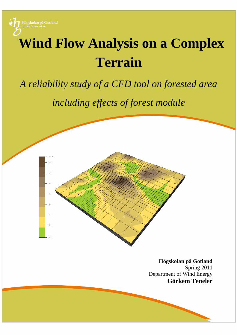
Wind Flow Analysis on a Complex
Terrain
A reliability study of a CFD tool on forested area
including effects of forest module
Högskolan på Gotland
Spring 2011
Department of Wind Energy
Görkem Teneler
Eventuell figur/bild (Formatmall: Figure and
picture text)
1
Wind Flow Analysis on a
Complex Terrain
A reliability study of a CFD tool on forested area
including effects of forest module
Master of Science Thesis
Wind Power Project Management
Spring 2011
GÖRKEM TENELER
Supervisor: Assoc. Dr. Stefan Ivanell
Co-supervisor: Karl J. Nilsson, MSc.
Examiner: Prof. Dr. Jens N. Sørensen
DEPARTMENT OF WIND ENERGY
GOTLAND UNIVERSITY
VISBY, SWEDEN, 2011
2
Abstract
The main aim of this thesis is to compare actual power production from an existing wind farm
with power production predicted by WindSim, which is a CFD tool based on a nonlinear flow
model. The wind farm in analysis is located in Northern Sweden and has high orographic
complexity with forested hilly terrain. There is 1 year record of met-mast wind measurements
and nearly 2 years record of production data.
Firstly, roughness and height data are given as input in order to simulate and generate the
wind fields over the complex terrain. In addition, the forest model is used to get more detailed
roughness height. After generating the wind fields, the existing turbine locations and 1-year
wind speed measurements are imported.
The results show how accurate the CFD calculations are to solve turbulence in complex
terrain. Comparison between actual production data and simulated energy production values
is the main approach of this thesis work to validate the simulations.
The results indicate that both WAsP and WindSim overestimate the energy production and the
wind speed. However, particularly when using the WindSim forest module, the CFD
calculations have more accurate results than the WAsP estimations.
Key words
Wind, Complex terrain, Forest, CFD, WindSim

3
Acknowledgments
This master of science thesis is the final project for the one year master`s program in Wind
Power Project Management at the Gotland University, Sweden. Examiner for the report is
Prof. Dr. Jens N. Sørensen from Technical University of Denmark, and the supervisor is
Assoc. Dr. Stefan Ivanell from Gotland University.
I would like to thank the academic staff in the department of wind energy at Gotland
University for providing this unique master education focused on wind power. Special thanks
to my thesis supervisor Assoc. Dr. Stefan Ivanell and also to Assoc. Dr. Bahri Uzunoğlu for
valuable suggestions.
Particular thanks to my second supervisor, Karl J. Nilsson and my classmate Raphael
Desilets-Aubé for their support and valuable discussion time.
I also thank you all my classmates and friends from other departments at Gotland University.
Lately I would like to give my most valuable thanks to my parents for their moral and
financial support during all my education life especially in Sweden.
Visby, September 2011
Görkem Teneler

4
Table of Contents Abstract ................................................................................................................................................... 2
Acknowledgments ................................................................................................................................... 3
Table of Contents .................................................................................................................................... 4
List of Figures ........................................................................................................................................... 6
List of Tables ............................................................................................................................................ 6
1 INTRODUCTION ........................................................................................................................... 7
1.1 Aim .......................................................................................................................................... 7
1.2 Question formulation ............................................................................................................... 8
1.3 Scientific methodology ............................................................................................................ 8
2 WIND .............................................................................................................................................. 9
2.1 Wind profile and shear ............................................................................................................ 9
2.2 Boundary layer ...................................................................................................................... 10
3 TOPOGRAPHY ............................................................................................................................ 12
3.1 Surface Roughness ................................................................................................................ 12
3.2 Obstacles ............................................................................................................................... 12
3.3 Terrain Orography ................................................................................................................. 12
3.4 Forest ..................................................................................................................................... 13
4 TURBULENCE ............................................................................................................................. 14
4.1 Turbulence intensity .............................................................................................................. 14
5 SIMULATION SITE ...................................................................................................................... 15
5.1 Terrain type and roughness ................................................................................................... 15
5.2 Orography and height contours ............................................................................................. 16
5.3 Wind conditions .................................................................................................................... 16
5.4 Wind turbines ........................................................................................................................ 16
6 METHODOLOGY ........................................................................................................................ 17
6.1 Terrain ................................................................................................................................... 17
6.1.1 Forest feature ................................................................................................................. 19
6.2 Wind Fields ........................................................................................................................... 20
6.3 Wind Data.............................................................................................................................. 22
6.4 Hardware ............................................................................................................................... 22
6.5 Software................................................................................................................................. 22
6.6 Test cases ............................................................................................................................... 23
7 RESULTS ...................................................................................................................................... 24

5
7.1 Wind resource and climatology ............................................................................................. 24
7.2 Wind profiles ......................................................................................................................... 25
7.3 Turbulence Intensity .............................................................................................................. 28
7.4 Wind shear exponent and wind speeds .................................................................................. 30
7.5 Annual Energy Production .................................................................................................... 31
8 DISCUSSION AND CONCLUSIONS ......................................................................................... 32
8.1 Terrain and wind data ............................................................................................................ 32
8.2 Wind speed ............................................................................................................................ 33
8.3 Energy production ................................................................................................................. 33
9 REFERENCES .................................................................................................................................. 35

6
List of Figures
Figure 2-1 Wind Profiles [6] ................................................................................................................. 10
Figure 2-2 Effect of roughness change on the atmospheric boundary layer [10] .................................. 10
Figure 2-3 Effects of roughness change on wind profiles [5] ............................................................... 11
Figure 3-1 Roughness length [6] ........................................................................................................... 12
Figure 3-2 Speed up effect [4] ............................................................................................................... 13
Figure 3-3 Flow inside and above forest canopy [9] ............................................................................. 13
Figure 5-1 Roughness map Figure 5-2 Height contours map ...................................... 15
Figure 5-3 Modelled terrain created in WindSim .................................................................................. 16
Figure 6-1 Sample of WindSim Terrain Module Properties table ......................................................... 17
Figure 6-2 Digital terrain model with refinement ................................................................................. 18
Figure 6-3 3D meshing with refinement ............................................................................................... 18
Figure 6-4 WindSim Forest Collection Editor ..................................................................................... 19
Figure 6-5 Roughness Map. .................................................................................................................. 20
Figure 6-6 Sample of WindSim Wind Field module properties table ................................................... 21
Figure 7-1 Wind frequency distribution Figure 7-2 Wind rose ................................................. 24
Figure 7-3 Wind resource map .............................................................................................................. 24
Figure 7-4 Wind profiles ....................................................................................................................... 25
Figure 7-5 Turbulence intensity ............................................................................................................ 28
List of Tables
Table 7-1 Wind speed results analysis .................................................................................................. 26
Table 7-2 Percentage difference between WindSim and WAsP wind speed predictions...................... 27
Table 7-3 TI results analysis ................................................................................................................. 29
Table 7-4 Wind speed, wind shear exponent and turbulence intensity analysis at met-mast location .. 30
Table 7-5 Annual energy production analysis ....................................................................................... 31
7
1 INTRODUCTION
Siting of turbines in complex land is becoming more and more common, although these areas
are not best sites, due to high shear and turbulence levels in the wind flow. Correct predictions
of flow are of great importance for the wind energy production. Forested and hilly areas are
normally characterized by large-scale heterogeneities, either due to the natural variation in the
landscape such as lakes and mires or due to clearings in the managed forests. These
heterogeneities add to the complexity of the flow. For forested hilly terrain, the prediction of
the separation of the flow above and below the boundary layer may be critical for assessing
the flow field around the hill correctly and therefore to optimize turbines location in order to
maximize energy output. These reasons can be cited for the increased importance of
simulation techniques in the recent years.
Computational Fluid Dynamics or simply CFD is concerned with obtaining numerical
solutions to the fluid flow problems using computers. The advent of high-speed and large-
memory computers has allowed CFD to get solutions for many flow problems including
compressible or incompressible, laminar or turbulent flows.
1.1 Aim
The main purpose of this study is to compare actual annual energy production from an
existing wind farm with power production values predicted using WindSim, which is a CFD
tool based on a nonlinear flow model.
The wind farm that is being worked on is located in Northern Sweden and has high
orographic complexity with forested hilly terrain. The complexity of the area makes flow over
the terrain harder to simulate using linear solvers. Furthermore, the farm is located in a
forested area; forest has significant effect on the flow by adding an internal boundary layer
and turbulence. For this reason, the additional forest module in WindSim is used to get more
accurate flow simulation.
There is about 1 year record of met-mast wind measurements and nearly 2 years record of
production data.
Firstly roughness and height data are given as input in order to simulate and generate wind
fields over the complex terrain. In addition, the forest model is used to get more detailed
8
roughness height. After generating the wind fields, the existing turbine locations and the 1-
year wind speed measurement are imported.
A comparison between actual production values from the wind farm and WAsP predicted
values (previously done by company), as well as WindSim simulation results is then
performed.
1.2 Question formulation
- How reliable is the CFD tool for the estimation of wind energy production specifically at
forested hilly terrain?
- How accurate is the CFD tool in modelling wind flow over complex terrain?
- How well does the forest module perform in representing the forest?
1.3 Scientific methodology
There are mainly three parts in the thesis:
- The theoretical part covers the theory about wind resource, boundary layer over complex
terrain, turbulence and flow models based on a literature study.
- The set-up and simulations part presents the compilation work performed based on the
data available from the existing farm.
- The analysis part presents simulation results and includes the comparison analysis
between energy estimation results and real production data.
9
2 WIND
The understanding of the characteristics of the wind is crucial in the development of wind
power especially in the choice of suitable sites and in the estimation of the energy production
regarding the economic feasibility of the wind farm projects.
The most significant characteristic of the wind is its unpredictability, both graphically and
temporally.
2.1 Wind profile and shear
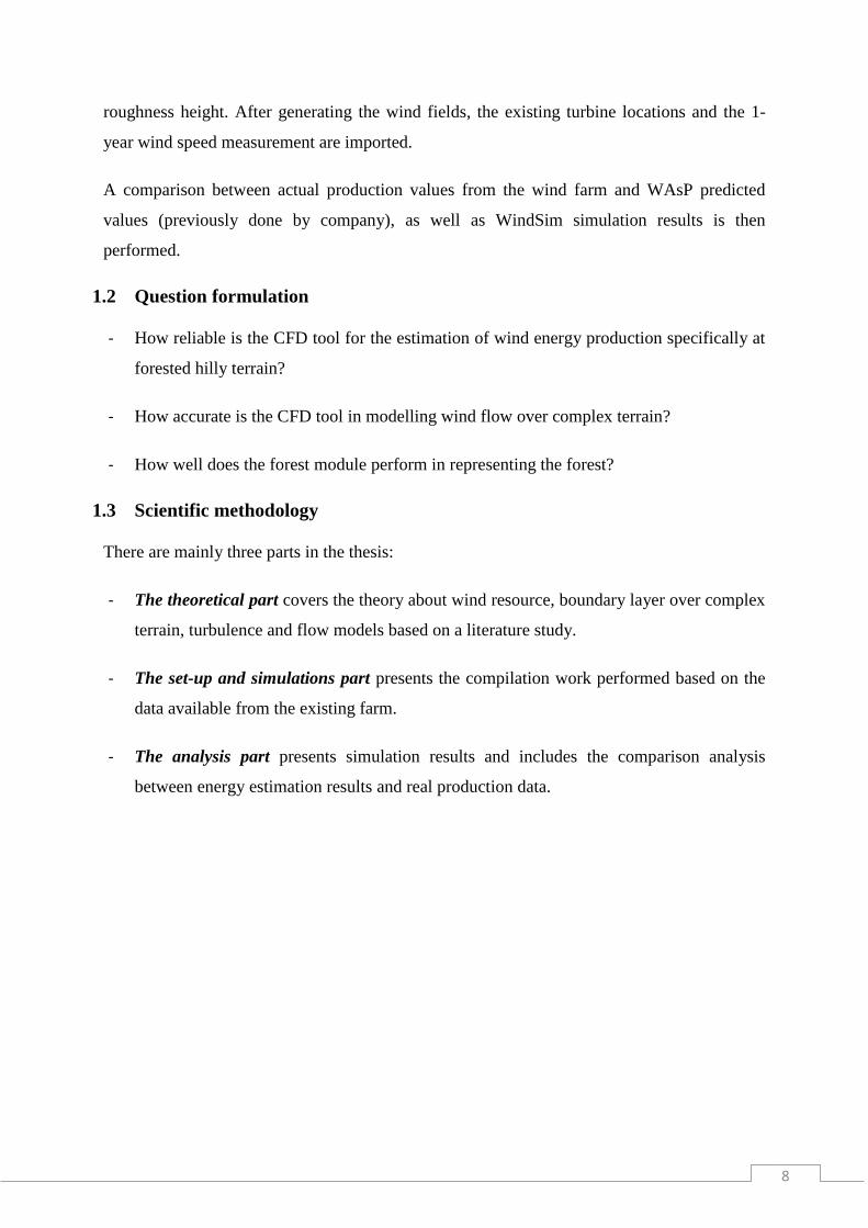
The relation between wind speed and height is called the wind profile. [8] The wind speed
increases with height. This increase depends on the friction against the surface. Over flat
terrain with low friction, the wind isn’t affected so much and the increase with height isn’t
very big. Over a surface with high roughness, the wind speed increases more significantly
with height.
Friction is stronger closer to the surface. For this reason the wind speed will decrease with
decreasing height and the wind direction changes as well across the isobars closer to the
surface. This change of wind speed and wind direction is called wind shear. [8]
The mean wind profile, that is basically wind speed as a function of height is often described
by the following approximation:
( )
( ) (
)
U (z1) and U (z2) are the wind speeds at heights z1 and z2;
p is the power law exponent, which varies with height, surface roughness and stability; for
this reason a more realistic expression for the wind speed as function of height z can be
obtained using the logarithmic wind profile:
10
Figure 2-1 Wind Profiles [6]
( ) (
)
u* is the friction velocity, k is the von Karman constant (≈ 0.4), z0 is the roughness length, and
φ is a stability-dependent function.
2.2 Boundary layer
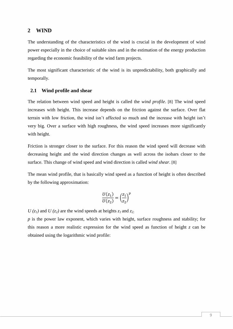
Friction is significant in the boundary layer. The velocity increases rapidly from zero at the
surface, to the value on the outer edge of the boundary layer.
Figure 2-2 Effect of roughness change on the atmospheric boundary layer [10]
The most straight forward definition of the location of the boundary layer’s upper edge is the
disturbance thickness δ; this is usually defined as the distance from the surface at which the
wind velocity u, is 99% of the free stream velocity U, that is, u ≈ 0.99U [1]
11
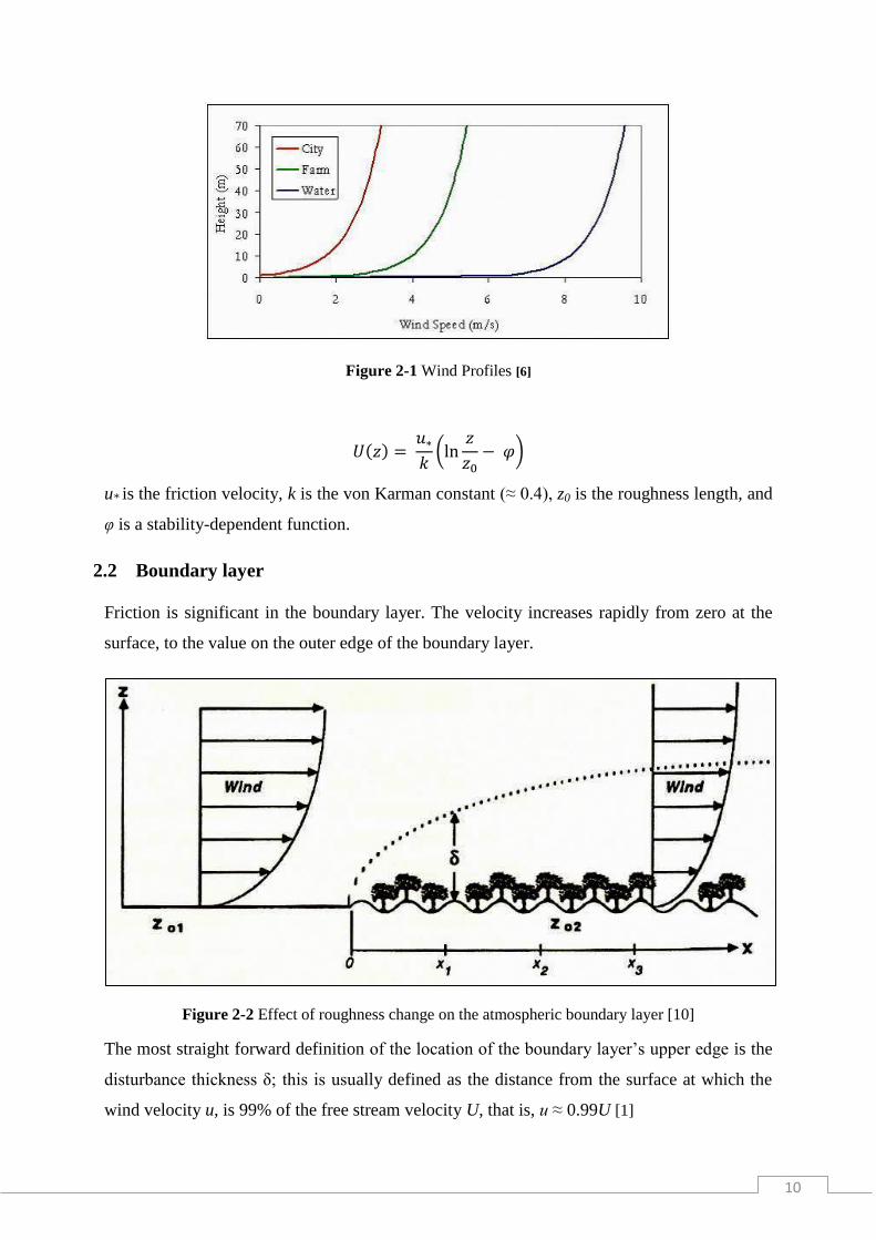
Figure 2-3 Effects of roughness change on wind profiles [5]
If the terrain conditions are not homogenous, that change affects the logarithmic wind profile.
The wind profile changes with roughness. Consequently, the height of the boundary layer
changes as well. Every new change of the location of the boundary layer causes the formation
of internal boundary layers.
( ⁄ )
( ⁄ )
is the friction velocity after the change, is before the change. h is the height of the
boundary layer. and represent roughness lengths before and after the profile change,
respectively.
12
3 TOPOGRAPHY
The wind is influenced by the Earth’s surface when it gets closer to the ground. In order to
better understand wind power meteorology, which is related to the wind flow up to 200
meters above the surface, three categories of the topography effects should be examined. [2]
3.1 Surface Roughness
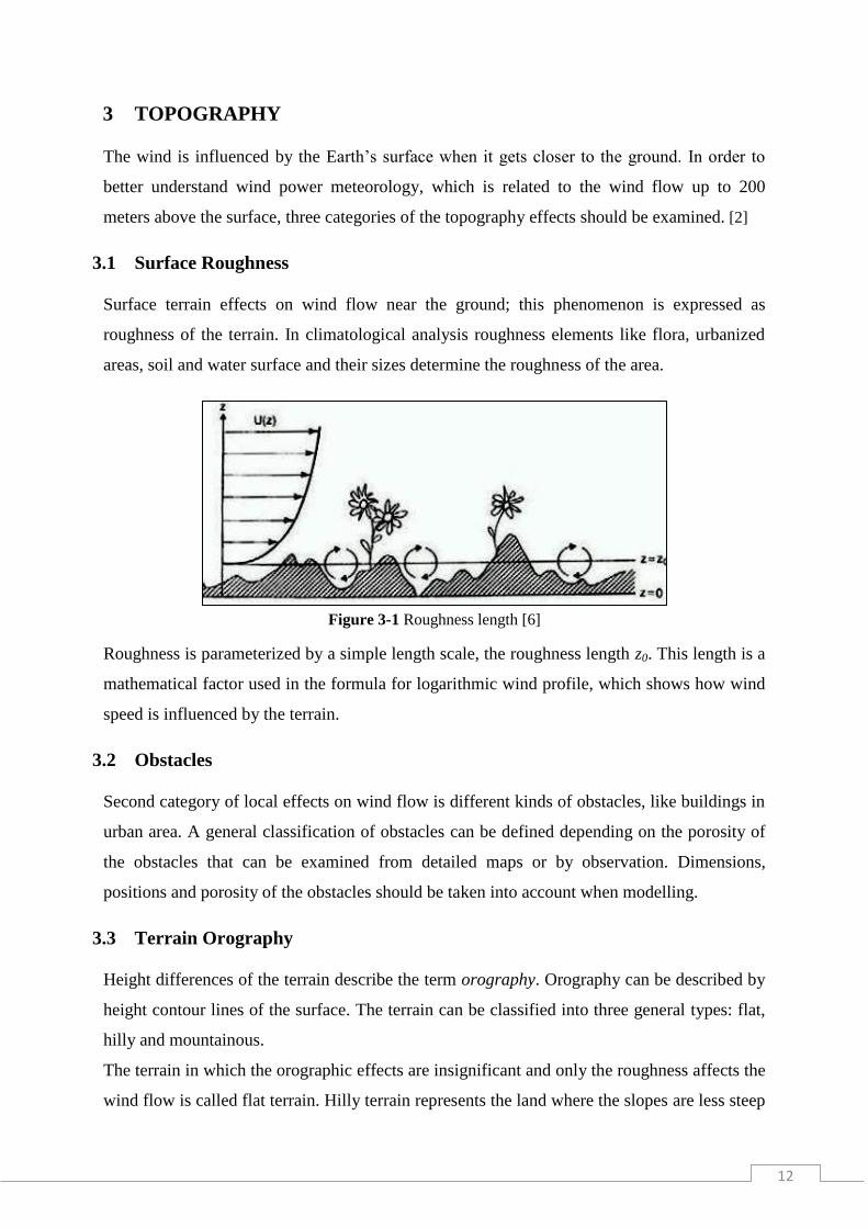
Surface terrain effects on wind flow near the ground; this phenomenon is expressed as
roughness of the terrain. In climatological analysis roughness elements like flora, urbanized
areas, soil and water surface and their sizes determine the roughness of the area.
Figure 3-1 Roughness length [6]
Roughness is parameterized by a simple length scale, the roughness length z0. This length is a
mathematical factor used in the formula for logarithmic wind profile, which shows how wind
speed is influenced by the terrain.
3.2 Obstacles
Second category of local effects on wind flow is different kinds of obstacles, like buildings in
urban area. A general classification of obstacles can be defined depending on the porosity of
the obstacles that can be examined from detailed maps or by observation. Dimensions,
positions and porosity of the obstacles should be taken into account when modelling.
3.3 Terrain Orography
Height differences of the terrain describe the term orography. Orography can be described by
height contour lines of the surface. The terrain can be classified into three general types: flat,
hilly and mountainous.
The terrain in which the orographic effects are insignificant and only the roughness affects the
wind flow is called flat terrain. Hilly terrain represents the land where the slopes are less steep
13
than about 0.3. [2] Hills have a significant influence on the wind speed. A smooth and not too
steep hill causes acceleration of the wind and makes the wind speed up when flowing towards
the hill top. The resultant increase in energy content is called hill impact.
Figure 3-2 Speed up effect [4]
In mountainous terrain, the slopes are steeper than in hilly terrain and it results on flow
separation. Terrain with high mountains and steep inclinations is called complex terrain. In
that type of terrain, the wind flow is very hard to predict and model by linear models. For this
reason non-linear models or measurements must be used.
3.4 Forest
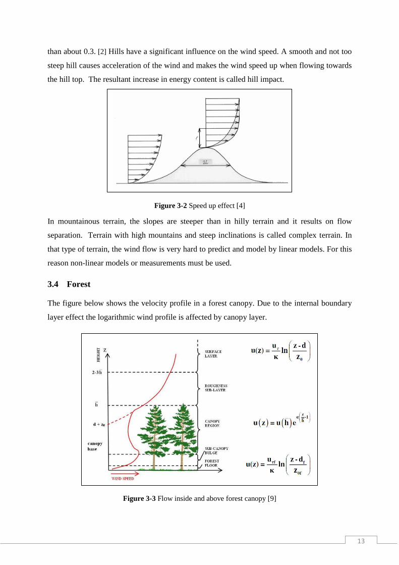
The figure below shows the velocity profile in a forest canopy. Due to the internal boundary
layer effect the logarithmic wind profile is affected by canopy layer.
Figure 3-3 Flow inside and above forest canopy [9]

14
4 TURBULENCE
The wind speed is naturally not stable. In other words, it fluctuates in short time scales,
typically less than 10 minutes. These variations of the wind speed are expressed in terms of
the standard deviation of the wind speed, σu. Turbulence refers to these fluctuations. Two
main causes generate turbulence: friction by the terrain surface, especially in hills and
mountains; and vertical air movement caused by temperature changes of the air.
It is clearly understood that turbulence is a complex phenomenon that cannot be defined in
terms of deterministic equations. In order to do that, physical laws such as conversation of
mass, momentum and energy, as well as descriptions of variation of temperature, pressure,
density, humidity and movement of air in three dimensions should be taken in to
consideration.[3] It makes turbulence more complex to understand well. Therefore, statistical
properties of turbulence are used to describe it.
4.1 Turbulence intensity
Turbulence intensity is one of the statistical properties that can be defined as the relation
between the standard deviation of the wind speed and the mean wind speed, that is,
Where σ is the standard deviation of the wind speed variations about the mean wind speed ,
often defined over 10 minutes or 1 hour. [8]
15
5 SIMULATION SITE
This thesis study was performed using data from a wind farm operated by a Swedish wind
power developer. In this section limited site information is presented in accordance to an
existent non-disclosure agreement.
5.1 Terrain type and roughness
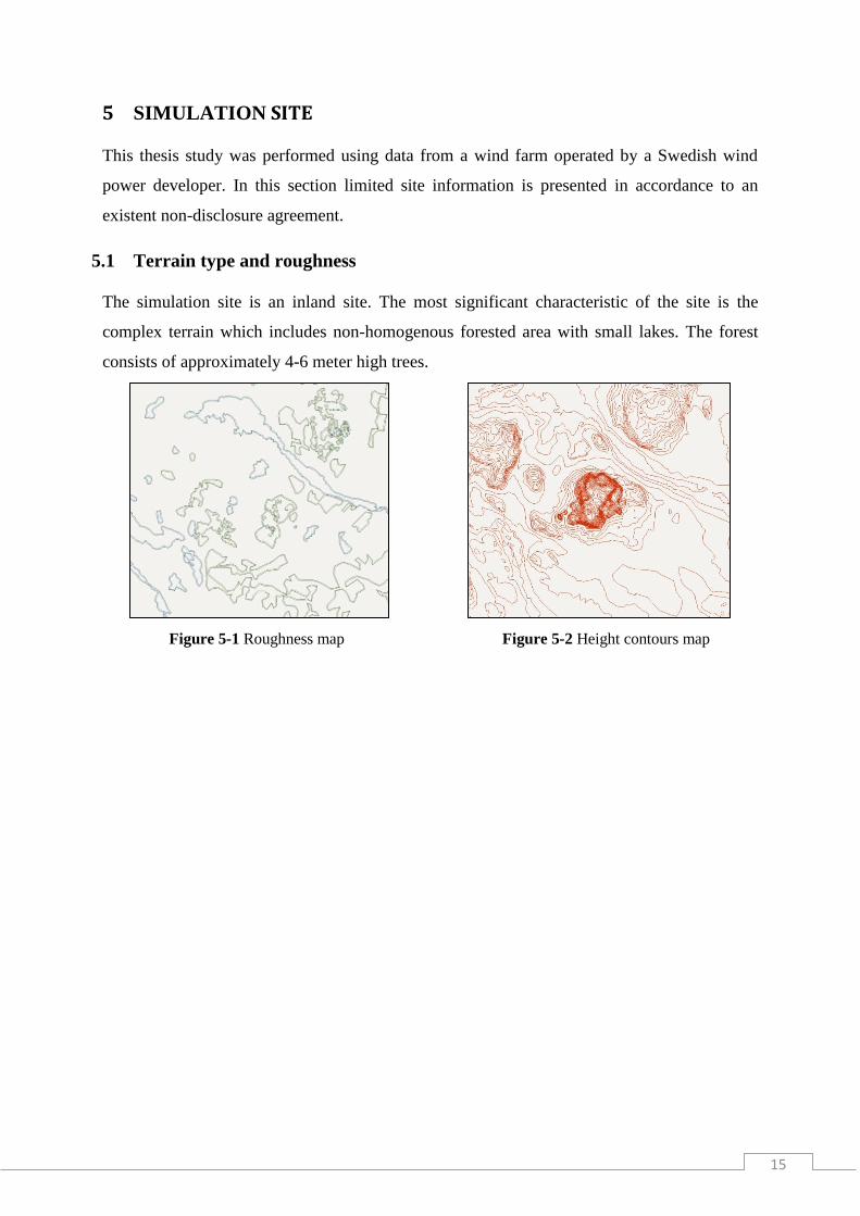
The simulation site is an inland site. The most significant characteristic of the site is the
complex terrain which includes non-homogenous forested area with small lakes. The forest
consists of approximately 4-6 meter high trees.
Figure 5-1 Roughness map Figure 5-2 Height contours map
16
5.2 Orography and height contours
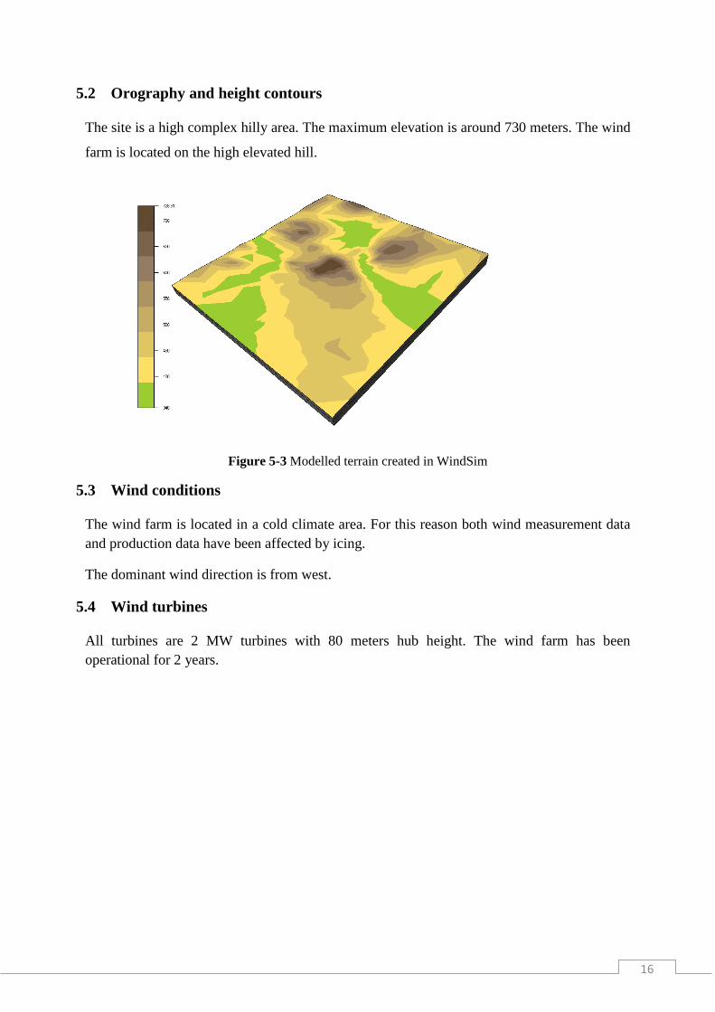
The site is a high complex hilly area. The maximum elevation is around 730 meters. The wind
farm is located on the high elevated hill.
Figure 5-3 Modelled terrain created in WindSim
5.3 Wind conditions
The wind farm is located in a cold climate area. For this reason both wind measurement data
and production data have been affected by icing.
The dominant wind direction is from west.
5.4 Wind turbines
All turbines are 2 MW turbines with 80 meters hub height. The wind farm has been
operational for 2 years.
17
6 METHODOLOGY
6.1 Terrain
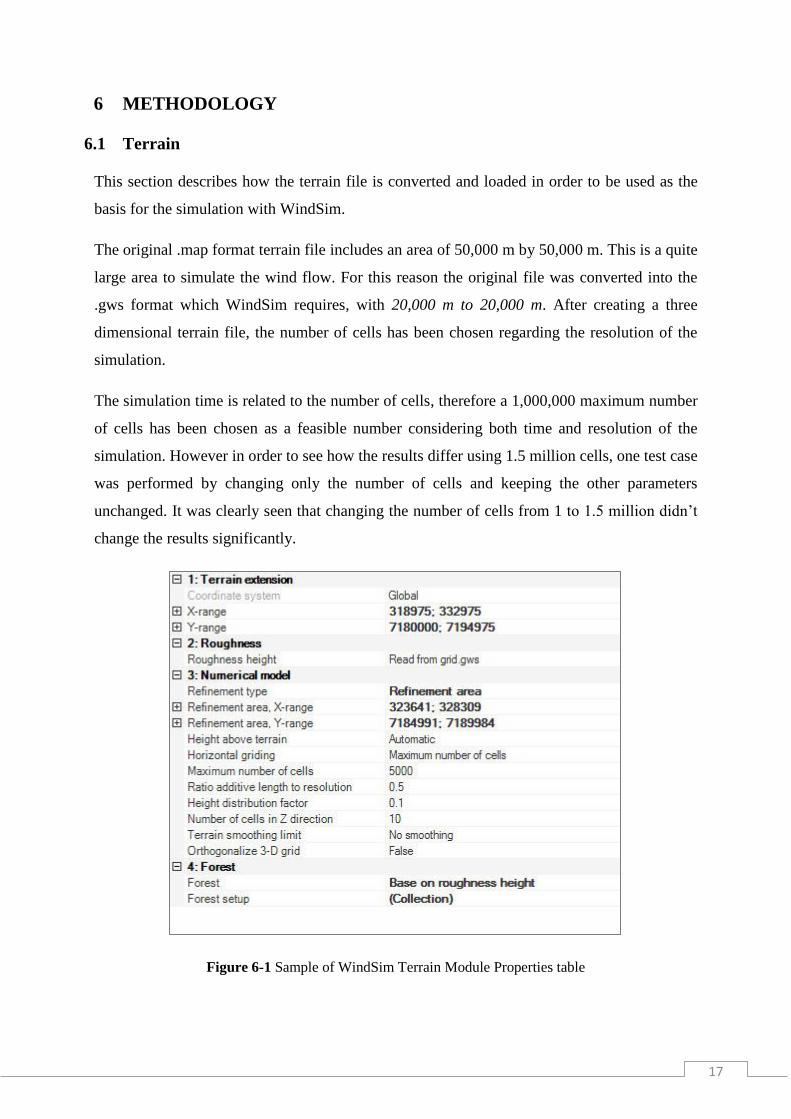
This section describes how the terrain file is converted and loaded in order to be used as the
basis for the simulation with WindSim.
The original .map format terrain file includes an area of 50,000 m by 50,000 m. This is a quite
large area to simulate the wind flow. For this reason the original file was converted into the
.gws format which WindSim requires, with 20,000 m to 20,000 m. After creating a three
dimensional terrain file, the number of cells has been chosen regarding the resolution of the
simulation.
The simulation time is related to the number of cells, therefore a 1,000,000 maximum number
of cells has been chosen as a feasible number considering both time and resolution of the
simulation. However in order to see how the results differ using 1.5 million cells, one test case
was performed by changing only the number of cells and keeping the other parameters
unchanged. It was clearly seen that changing the number of cells from 1 to 1.5 million didn’t
change the results significantly.
Figure 6-1 Sample of WindSim Terrain Module Properties table
18
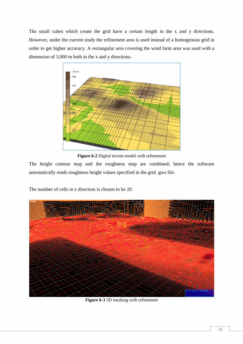
The small cubes which create the grid have a certain length in the x and y directions.
However, under the current study the refinement area is used instead of a homogenous grid in
order to get higher accuracy. A rectangular area covering the wind farm area was used with a
dimension of 3,000 m both in the x and y directions.
Figure 6-2 Digital terrain model with refinement
The height contour map and the roughness map are combined; hence the software
automatically reads roughness height values specified in the grid .gws file.
The number of cells in z direction is chosen to be 20.
Figure 6-3 3D meshing with refinement
19
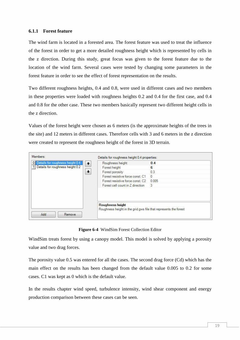
6.1.1 Forest feature
The wind farm is located in a forested area. The forest feature was used to treat the influence
of the forest in order to get a more detailed roughness height which is represented by cells in
the z direction. During this study, great focus was given to the forest feature due to the
location of the wind farm. Several cases were tested by changing some parameters in the
forest feature in order to see the effect of forest representation on the results.
Two different roughness heights, 0.4 and 0.8, were used in different cases and two members
in these properties were loaded with roughness heights 0.2 and 0.4 for the first case, and 0.4
and 0.8 for the other case. These two members basically represent two different height cells in
the z direction.
Values of the forest height were chosen as 6 meters (is the approximate heights of the trees in
the site) and 12 meters in different cases. Therefore cells with 3 and 6 meters in the z direction
were created to represent the roughness height of the forest in 3D terrain.
Figure 6-4 WindSim Forest Collection Editor
WindSim treats forest by using a canopy model. This model is solved by applying a porosity
value and two drag forces.
The porosity value 0.5 was entered for all the cases. The second drag force (Cd) which has the
main effect on the results has been changed from the default value 0.005 to 0.2 for some
cases. C1 was kept as 0 which is the default value.
In the results chapter wind speed, turbulence intensity, wind shear component and energy
production comparison between these cases can be seen.

20
Figure 6-5 Roughness Map.
(Forest is represented by grey cells by the canopy model)
6.2 Wind Fields
WindSim has a second module where user determines the boundary conditions such as the
number of sections, the boundary layer (BL) height and the speed above the BL height. In
addition, some important physical properties can be chosen in this section. Air density and
turbulence models are parts of this module. After generating a 3D model with the terrain
feature, the properties of wind fields were entered.
For all cases the number of wind sectors was selected to be 12 which is equal to the number of
sectors used in the climatology. The wind sectors were distributed uniformly. The height of
the boundary layer was defined as 1000m (default value is 500m) and the velocity above
boundary layer was set to 12 m/s.
The potential temperature was disregarded.
An inland and forested area has a different air density as compared to an offshore or coastal
area. Previous simulations were done by the developer with WAsP, where the air density
21
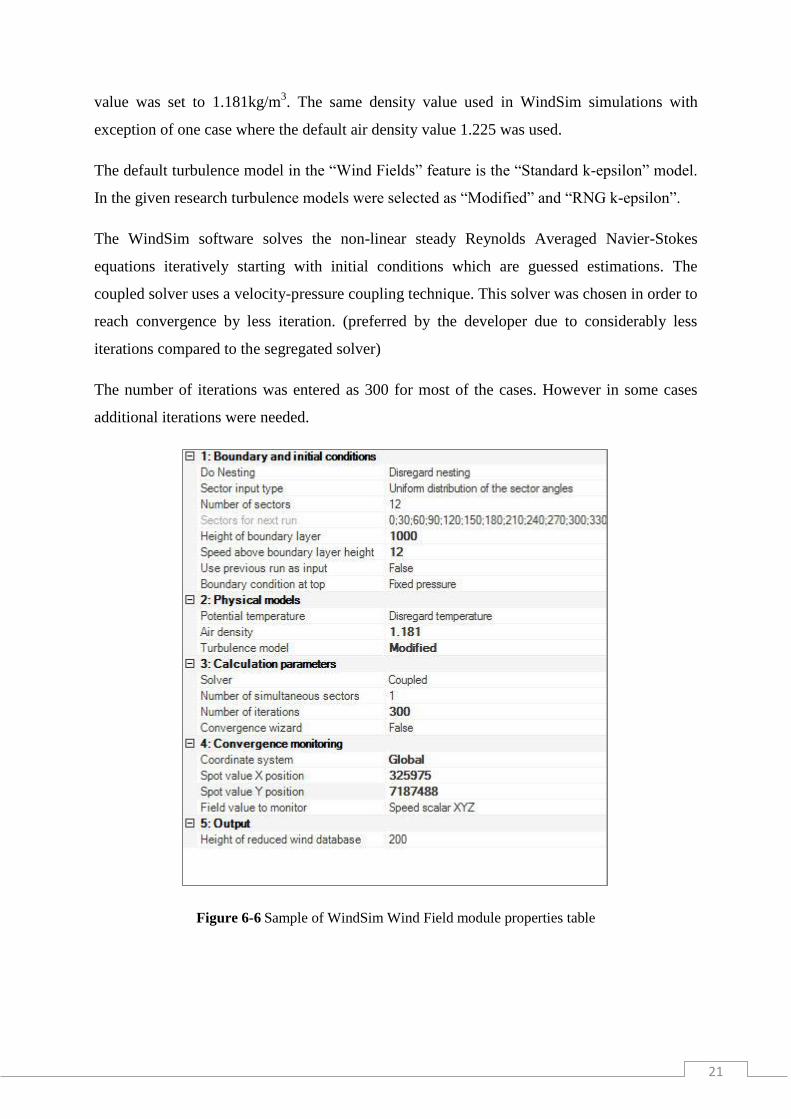
value was set to 1.181kg/m3. The same density value used in WindSim simulations with
exception of one case where the default air density value 1.225 was used.
The default turbulence model in the “Wind Fields” feature is the “Standard k-epsilon” model.
In the given research turbulence models were selected as “Modified” and “RNG k-epsilon”.
The WindSim software solves the non-linear steady Reynolds Averaged Navier-Stokes
equations iteratively starting with initial conditions which are guessed estimations. The
coupled solver uses a velocity-pressure coupling technique. This solver was chosen in order to
reach convergence by less iteration. (preferred by the developer due to considerably less
iterations compared to the segregated solver)
The number of iterations was entered as 300 for most of the cases. However in some cases
additional iterations were needed.
Figure 6-6 Sample of WindSim Wind Field module properties table
22
6.3 Wind Data
The wind data provided by the developer is from a met mast which measured the wind before
the installation of the turbines. For wind resource assessments, a minimum of 12 months
measurement is recommended. In the given study, 1 year of met mast measurements is used.
The mast measurement data correspond to a 49.7 meters height and include 10 minutes
average wind speed and wind direction for a 1 year period.
However the wind data was influenced by icing due to cold climate mainly in winter time. For
this reason, icing periods were identified and removed from the measured data by the
developer company. Therefore, there are two wind data sets for the same time period: the
original dataset and the cleaned dataset.
The company used cleaned data for power production estimation using WAsP. In order to
compare the results obtained from both softwares, cleaned data were used as well in this
study.
6.4 Hardware
Similarly to most of the commercial and very computationally intensive CFD tools, WindSim
requires high end strong computing resources with enough memory to run a model of large
size. The computer which was used for simulations has Intel Core i7 quad-core processors
with 16GB of fast 1333 MHz (DDR3) memory.
6.5 Software
WindSim version 5.0.1 was used. For 3D images WindSim GL view Pro 6.3-42 version was
used.
The software licence was procured by the Gotland University as an academic license under an
agreement between the university and the software developer.
23
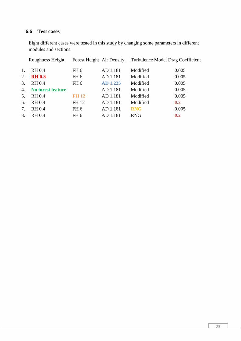
6.6 Test cases
Eight different cases were tested in this study by changing some parameters in different
modules and sections.
Roughness Height Forest Height Air Density Turbulence Model Drag Coefficient
1. RH 0.4 FH 6 AD 1.181 Modified 0.005
2. RH 0.8 FH 6 AD 1.181 Modified 0.005
3. RH 0.4 FH 6 AD 1.225 Modified 0.005
4. No forest feature AD 1.181 Modified 0.005
5. RH 0.4 FH 12 AD 1.181 Modified 0.005
6. RH 0.4 FH 12 AD 1.181 Modified 0.2
7. RH 0.4 FH 6 AD 1.181 RNG 0.005
8. RH 0.4 FH 6 AD 1.181 RNG 0.2
24
7 RESULTS
7.1 Wind resource and climatology
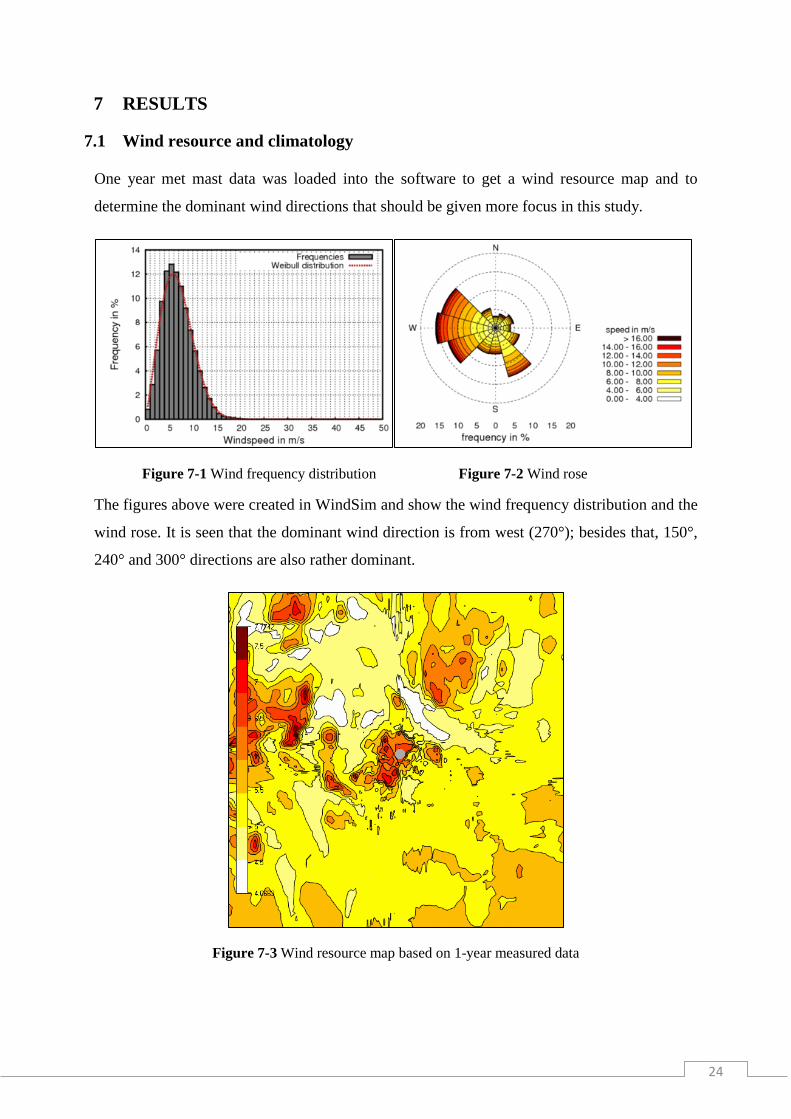
One year met mast data was loaded into the software to get a wind resource map and to
determine the dominant wind directions that should be given more focus in this study.
Figure 7-1 Wind frequency distribution Figure 7-2 Wind rose
The figures above were created in WindSim and show the wind frequency distribution and the
wind rose. It is seen that the dominant wind direction is from west (270°); besides that, 150°,
240° and 300° directions are also rather dominant.
Figure 7-3 Wind resource map based on 1-year measured data
25
7.2 Wind profiles
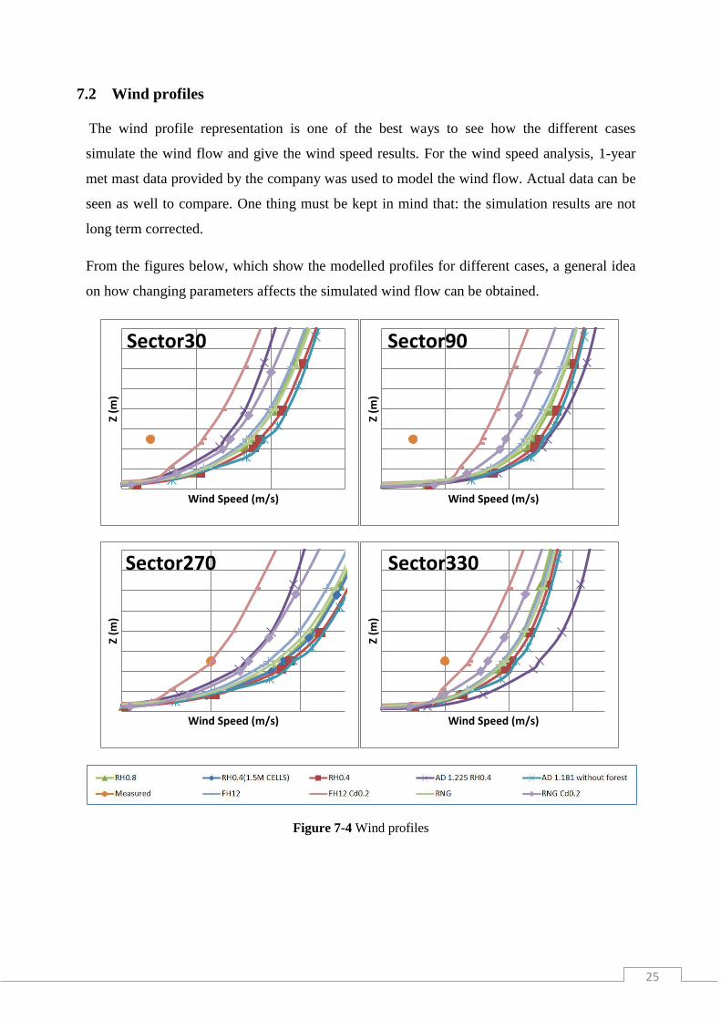
The wind profile representation is one of the best ways to see how the different cases
simulate the wind flow and give the wind speed results. For the wind speed analysis, 1-year
met mast data provided by the company was used to model the wind flow. Actual data can be
seen as well to compare. One thing must be kept in mind that: the simulation results are not
long term corrected.
From the figures below, which show the modelled profiles for different cases, a general idea
on how changing parameters affects the simulated wind flow can be obtained.
Figure 7-4 Wind profiles
Z (m
)
Wind Speed (m/s)
Sector30
Z (m
)
Wind Speed (m/s)
Sector90
Z (m
)
Wind Speed (m/s)
Sector270
Z (m
)
Wind Speed (m/s)
Sector330
26
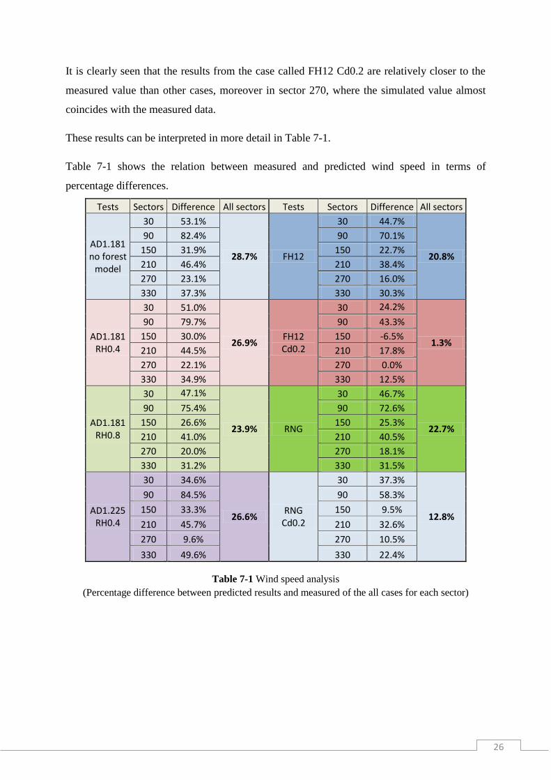
It is clearly seen that the results from the case called FH12 Cd0.2 are relatively closer to the
measured value than other cases, moreover in sector 270, where the simulated value almost
coincides with the measured data.
These results can be interpreted in more detail in Table 7-1.
Table 7-1 shows the relation between measured and predicted wind speed in terms of
percentage differences.
Tests Sectors Difference All sectors Tests Sectors Difference All sectors
AD1.181 no forest
model
30 53.1%
28.7% FH12
30 44.7%
20.8%
90 82.4% 90 70.1%
150 31.9% 150 22.7%
210 46.4% 210 38.4%
270 23.1% 270 16.0%
330 37.3% 330 30.3%
AD1.181 RH0.4
30 51.0%
26.9% FH12 Cd0.2
30 24.2%
1.3%
90 79.7% 90 43.3%
150 30.0% 150 -6.5%
210 44.5% 210 17.8%
270 22.1% 270 0.0%
330 34.9% 330 12.5%
AD1.181 RH0.8
30 47.1%
23.9% RNG
30 46.7%
22.7%
90 75.4% 90 72.6%
150 26.6% 150 25.3%
210 41.0% 210 40.5%
270 20.0% 270 18.1%
330 31.2% 330 31.5%
AD1.225 RH0.4
30 34.6%
26.6% RNG
Cd0.2
30 37.3%
12.8%
90 84.5% 90 58.3%
150 33.3% 150 9.5%
210 45.7% 210 32.6%
270 9.6% 270 10.5%
330 49.6% 330 22.4%
Table 7-1 Wind speed analysis
(Percentage difference between predicted results and measured of the all cases for each sector)
27
A main conclusion from these results is that without using forest module the results are rather
higher than cases with forest module. Furthermore, when it comes to cases with forest height
(FH) and drag coefficient (Cd), which are the main factors of the canopy model, the
percentage difference are smaller; it means that predicted results are closer to the measured
data.
It appears that the forest canopy model, especially when drag coefficient was changed,
worked well.
WindSim
AD1.225 RH0.4
AD1.181 RH0.4
AD1.181 RH0.8
AD1.181 no forest
FH12 FH12 Cd0.2
FH12 RNG
RNG Cd0.2
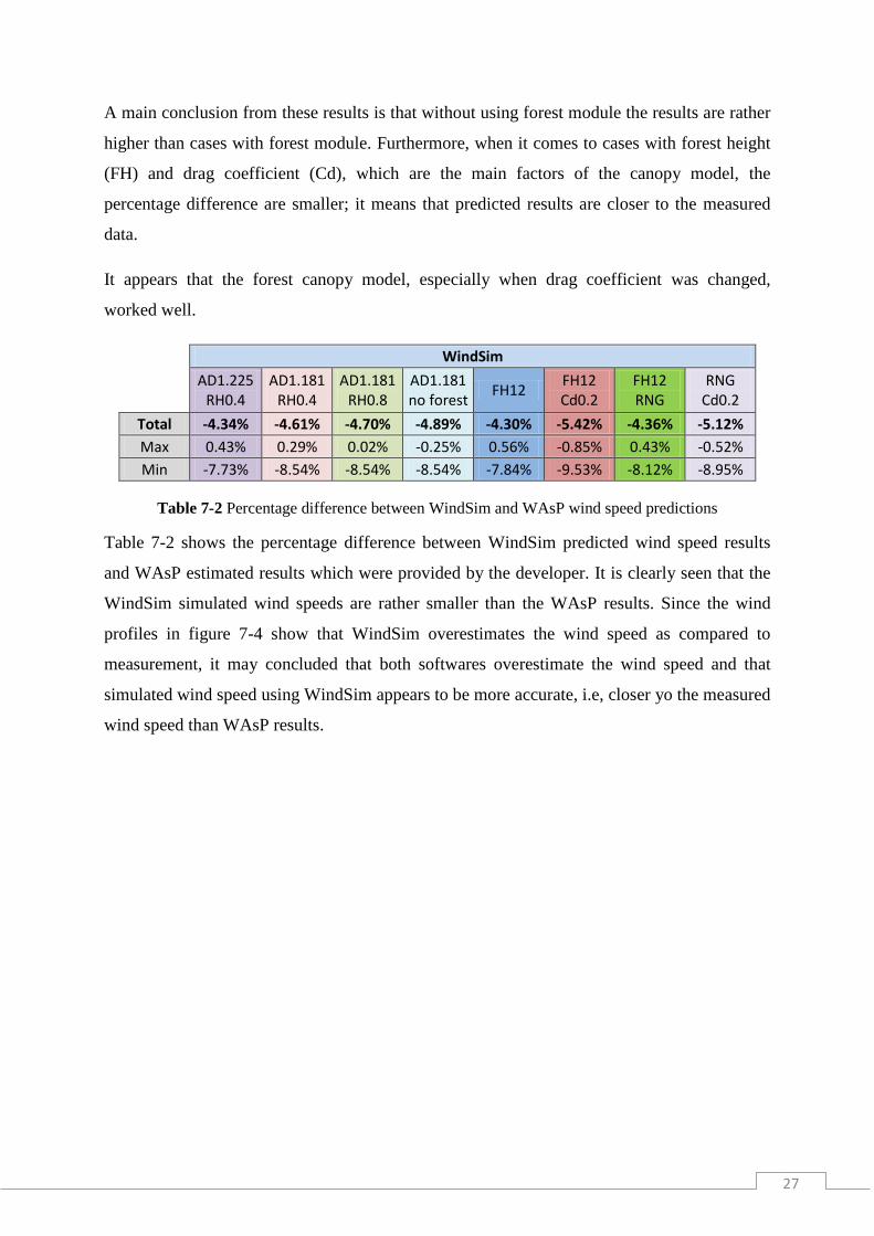
Total -4.34% -4.61% -4.70% -4.89% -4.30% -5.42% -4.36% -5.12%
Max 0.43% 0.29% 0.02% -0.25% 0.56% -0.85% 0.43% -0.52%
Min -7.73% -8.54% -8.54% -8.54% -7.84% -9.53% -8.12% -8.95%
Table 7-2 Percentage difference between WindSim and WAsP wind speed predictions
Table 7-2 shows the percentage difference between WindSim predicted wind speed results
and WAsP estimated results which were provided by the developer. It is clearly seen that the
WindSim simulated wind speeds are rather smaller than the WAsP results. Since the wind
profiles in figure 7-4 show that WindSim overestimates the wind speed as compared to
measurement, it may concluded that both softwares overestimate the wind speed and that
simulated wind speed using WindSim appears to be more accurate, i.e, closer yo the measured
wind speed than WAsP results.
28
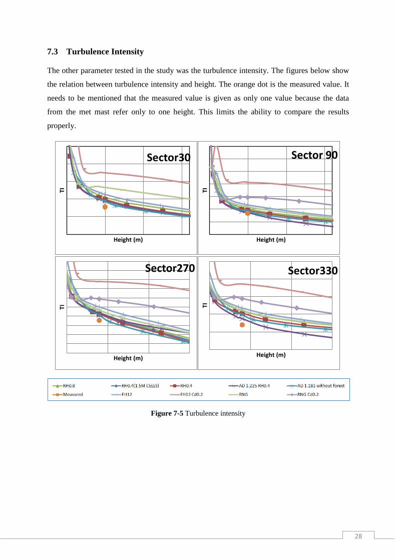
7.3 Turbulence Intensity
The other parameter tested in the study was the turbulence intensity. The figures below show
the relation between turbulence intensity and height. The orange dot is the measured value. It
needs to be mentioned that the measured value is given as only one value because the data
from the met mast refer only to one height. This limits the ability to compare the results
properly.
Figure 7-5 Turbulence intensity
TI
Height (m)
Sector30
TI
Height (m)
Sector 90
TI
Height (m)
Sector270
TI
Height (m)
Sector330
29
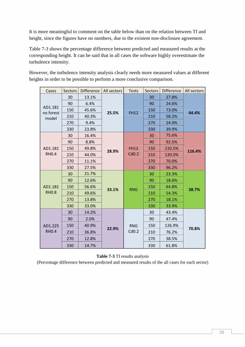
It is more meaningful to comment on the table below than on the relation between TI and
height, since the figures have no numbers, due to the existent non-disclosure agreement.
Table 7-3 shows the percentage difference between predicted and measured results at the
corresponding height. It can be said that in all cases the software highly overestimate the
turbulence intensity.
However, the turbulence intensity analysis clearly needs more measured values at different
heights in order to be possible to perform a more conclusive comparison.
Cases Sectors Difference All sectors Tests Sectors Difference All sectors
AD1.181 no forest
model
30 13.1%
25.5% FH12
30 27.8%
44.4%
90 6.4% 90 24.6%
150 45.6% 150 73.0%
210 40.3% 210 58.2%
270 9.4% 270 24.0%
330 23.8% 330 39.9%
AD1.181 RH0.4
30 16.4%
28.9% FH12 Cd0.2
30 75.6%
116.4%
90 8.8% 90 92.5%
150 49.8% 150 210.5%
210 44.0% 210 120.0%
270 11.1% 270 70.0%
330 27.5% 330 96.2%
AD1.181 RH0.8
30 21.7%
33.1% RNG
30 23.3%
38.7%
90 12.6% 90 18.6%
150 56.6% 150 64.8%
210 49.6% 210 54.3%
270 13.8% 270 18.1%
330 33.0% 330 33.9%
AD1.225 RH0.4
30 14.2%
22.9% RNG
Cd0.2
30 43.4%
70.8%
90 2.0% 90 47.4%
150 40.9% 150 126.9%
210 36.8% 210 76.2%
270 12.8% 270 38.5%
330 14.7% 330 61.8%
Table 7-3 TI results analysis
(Percentage difference between predicted and measured results of the all cases for each sector)

30
7.4 Wind shear exponent and wind speeds
In this section of the results part, a general conclusion is given by the table below for the all
cases and including wind shear exponent analysis.
Case
AD1.181 RH0.4
AD1.181 RH0.8
AD1.225 RH0.4
AD1.181 no forest
FH12 FH12 Cd0.2
RNG RNG
Cd0.2
Speed_2D 26.9% 23.9% 26.6% 28.7% 20.8% 1.3% 22.7% 12.8%
Shear Exp.
20.6% 20.5% 24.0% 27.2% 18.8% 17.2% 17.6% 25.4%
TI 28.9% 33.1% 22.9% 25.5% 44.4% 116.4% 38.7% 70.8%
Table 7-4 Wind speed, wind shear exponent and turbulence intensity analysis at met-mast location
(Percentage difference between predicted and measured results)
As it can be seen from table the above, WindSim overpredicts the results for almost all the
cases and for all the parameters.
For wind speed and wind shear exponent results, especially in the cases when the canopy
model was used, the percentage difference is lower. However, the deviation between
simulated and measured turbulence intensity is rather large for these cases.
These results are further discussed in the Discussion section.

31
7.5 Annual Energy Production
The WindSim simulation is performed with and without wake interaction between turbines.
Since the wind farm has several turbines, the results with wake interaction will be presented
in the study. The company has previously done a simulation of the expected production using
WAsP. Furthermore, available actual annual production data was provided. The table below
compares measured actual production with both WAsP and WindSim predicted annual energy
production values.
There are 3 different representations of the analysis with total, max and min. Total means
percentage difference of the estimated production for the whole farm including all turbines.
Max and min values are the results obtained for singular turbines.
WAsP
(AD1.181)
WindSim
AD1.225 RH0.4
AD1.181 RH0.4
AD1.181 RH0.8
AD1.181 no forest
FH12 FH12 Cd0.2
FH12 RNG
RNG Cd0.2
Total 12.68% 15.14% 12.15% 14.54% 11.47% 12.86% 10.36% 12.75% 11.17%
Max 25.11% 25.36% 22.23% 25.01% 21.42% 22.93% 20.89% 22.81% 21.21%
Min 0.89% 3.08% -1.28% 1.14% -1.63% -0.35% -2.21% -0.50% -0.92%
Table 7-5 Annual energy production analysis
(Percentage difference between predicted results by both softwares and actual production results)
The results show that WAsP overestimated the total energy production of the farm with
12.68%. Although for one turbine the estimated production using WAsP is almost the same as
the actual production. However there is a rather high overestimation for another turbine
(25.11%).
Eight different cases were tested to get more accurate estimations. It can be seen from the
Table 7-5 that different cases corresponding to different parameters change the results
significantly. Although WindSim simulation results also highly overestimate the production,
half of the cases have rather lower overestimation than the WAsP results.
It should be mentioned that the most accurate estimation is the case when the canopy model
was applied with FH12 and Cd0.2 (see Section 6.6 for the definition of the different test
cases). This means that the use of canopy model is appropriate for the simulation of the
energy production of this wind farm, that is, indeed, located on a forested area.
32
8 DISCUSSION AND CONCLUSIONS
The wind farm in analysis is located on a forested area with hilly terrain. The impact of the
hilly terrain and of the forested surface makes the simulation of the wind flow to be complex.
Hence, the focus of this study is to model the wind flow by testing different parameters and
by trying to find accurate estimations over complex terrain.
Starting with the definition of the climatology and of the simulations for wind speed,
turbulence intensity and annual energy production, it was the given at attempt to get the
answers for the questions “How reliable is the CFD tool for estimation wind energy
production specifically at forested hilly terrain?” and “How accurate is the CFD tool to model
wind flow over complex terrain?”
8.1 Terrain and wind data
Terrain and wind data of the wind farm were provided by the company.
Terrain data includes height contours and roughness data. Especially after modelling the
forest by the WindSim software it was clearly seen that the roughness data wasn’t detailed
enough to represent the complexity of the forest. Therefore the forest module couldn’t work
properly. There is the need to define the properties of the forest using parameters such as
forest height, porosity etc.
There are one-year wind measurements available. The wind measurements were cleaned for
icing events.
Wind data is measured only at one height. This fact limits the possibilities of testing the
results from the CFD simulations.

33
8.2 Wind speed
Wind speed is the parameter that can help finding an answer to the question “how well does
the CFD tool model the wind flow?” There are 8 different test cases. After running
simulations for each of them wind profiles were created in WindSim software, see section 7.2.
Both from profiles and table that show percentage difference between measured and predicted
results it can be said that generally the results are overestimated by WindSim. The main
approach using the canopy model by changing the forest height and the drag coefficient works
well. The closest results are given by the canopy model with FH12 and Cd0.2.
This conclusion reinforces the importance of using a canopy model when modelling the wind
flow in forested terrain and of defining the forest properties properly.
8.3 Energy production
The main goal of testing different simulation cases is to get accurate energy production
estimations. It is crucial for the wind energy industry to predict well. Therefore simulation
results for energy production are the final step of this study.
The company performed production estimation prior to the construction of the wind farm. The
software used was WAsP which is known as a linear solver. The WAsP model is generally
used for wind farm in rather less complex terrain. CFD solvers are on the other hand getting
more popular for complex areas.
Both WindSim and WAsP simulation results overestimate the wind speed and the actual
annual production as shown in Section 7.5. However, using the canopy model one gets more
accurate results, i.e., the estimated values are closer to the actual measured results
For both cases there should be some losses due to the other factors that the software does not
take into consideration.
The wind farm is located in a cold climate area. It is known that icing affects the production
results with around 10% loss. After this assumption, the simulation results seem more realistic
and closer to the actual values.

34
Overall for further studies in the field of this study, it is recommended the following:
To get more detailed terrain data especially for forested area.
To get more information about forest properties (tree type, porosity, forest height)
To improve the variety and quantity of the measurements
To work on single turbine instead of whole farm might give better energy comparison
To provide production data for each sector could give a more accurate comparison
Cold climate effects should be taken into consideration by more accurate corrections.
35
9 REFERENCES
[1] W.Fox Alan T.McD, Introduction to Fluid Mechnanics, 6th
edition, 2004.
[2] E.L. Petersen, Wind Power Meteorology, Risoe-1-1206(EN), 2007.
[3] T. Burton, D.Sharpe, N.Jenkins, Wind Energy Handbook, 2001.
[4] T. Wallbank, WindSim Validation Study, 2008.
[5] K.J. Nilsson, A reliability study of two conventional computer software, Master Thesis at
Chalmers University and Gotland University, 2010.
[6] A.Crockford, S-Y Hui, Wind profiles and forests, Master Thesis at Risoe DTU, 2007.
[7] C.Meissner, WindSim Getting Started, 5 th
edition, 2010.
[8] T.Wizelius, Developing Wind Power Projects, 2007.
[9] G.Crasto, Numerical simulations of the atmospheric boundary layer, 2007.
[10] R.B. Stull, An Introduction to Boundary Layer Meteorology, 1988.