Embed Size (px)
Citation preview

University of Calgary
PRISM: University of Calgary's Digital Repository
Graduate Studies The Vault: Electronic Theses and Dissertations
2017
Wind Farm Layout Optimization Considering
Commercial Turbine Selection and Hub Height
Variation
Abdulrahman, Mamdouh Ahmad
Abdulrahman, M. A. (2017). Wind Farm Layout Optimization Considering Commercial Turbine
Selection and Hub Height Variation (Unpublished doctoral thesis). University of Calgary, Calgary,
AB. doi:10.11575/PRISM/28711
http://hdl.handle.net/11023/4118
doctoral thesis
University of Calgary graduate students retain copyright ownership and moral rights for their
thesis. You may use this material in any way that is permitted by the Copyright Act or through
licensing that has been assigned to the document. For uses that are not allowable under
copyright legislation or licensing, you are required to seek permission.
Downloaded from PRISM: https://prism.ucalgary.ca

UNIVERSITY OF CALGARY
Wind Farm Layout Optimization Considering Commercial Turbine Selection and Hub Height
Variation
by
Mamdouh Ahmad Abdulrahman
A THESIS
SUBMITTED TO THE FACULTY OF GRADUATE STUDIES
IN PARTIAL FULFILMENT OF THE REQUIREMENTS FOR THE
DEGREE OF DOCTOR OF PHILOSOPHY
GRADUATE PROGRAM IN MECHANICAL AND MANUFACTURING ENGINEERING
CALGARY, ALBERTA
SEPTEMBER, 2017
© Mamdouh Ahmad Abdulrahman 2017

ii
Abstract
New aspects were added to the wind farm layout optimization problem; commercial turbine
selection, generic realistic representation for the thrust coefficient, investigating the power-cost of
energy trade-off range, and introducing the wind farm layout upgrade optimization problem. A
range of commercial turbines was selected and the manufacturers’ power curves were used to
evaluate the power developed by each turbine using the effective wind speed. The classical
Jensen’s wake model was implemented to simulate the wake and wake interference within the
farm in an analytic and accurate way. A simple field-based cost model was developed to evaluate
the cost of any layout in terms of the turbine rated power and hub height. For the upgrade cases,
the cost model included an area factor to account the upgraded area to the original farm area. A
Genetic Algorithm was used for optimization throughout this dissertation. A technique called
Random Independent Multi-Population Genetic Algorithm was used in some cases to accelerate
the optimization.
The results showed that co-operative optimization is superior over the selfish one. The turbine
aerodynamic efficiency was found to magnify the difference between the two optimization
strategies. A wide range of commercial turbines was selected and a useful range of power-cost of
energy trade-off was obtained. The optimization was found to be more efficient in offshore cases
because of the low entrainment coefficient in the wake model. The Random Independent Multi-
Population technique caused a significant reduction in the speed of the optimization. It is likely
that most farms can be efficiently and practically upgraded with a wide range of power-cost of
energy trade-offs, using the proposed upgrade layout and the optimization objective.

iii
Keywords: Wind farm layout optimization, Layout upgrade optimization, Commercial turbine
selection, Hub height variation, Multi-population genetic algorithm, Thrust coefficient,
Aerodynamic efficiency, Co-operative optimization, Selfish optimization.

iv
Preface
This thesis collects the research conducted by the candidate under the supervision of Professor
D.H. Wood in the field of Wind Farm Layout Optimization (WFLO). Chapter 3, Chapter 4, and
Chapter 5 have been published, the citations are:
▪ Kiani, A., Abdulrahman, M., Wood, D. (2014). Explicit solutions for simple models of
wind turbine interference. Wind Engineering, 38(2), pp. 167-180.
▪ Abdulrahman, M., Wood, D. (2015). Some effects of efficiency on wind turbine
interference and maximum power production. Wind Engineering, 39(5), pp. 495-506.
▪ Abdulrahman, M., Wood, D. (2017). Investigating the power-COE trade-off for wind
farm layout optimization considering commercial turbine selection and hub height
variation. Renewable Energy, 102 (B) (2017) 267-516.
Chapter 6 has revised and resubmitted to Renewable Energy and is under review:
▪ Abdulrahman, M., Wood, D. (2017). Large wind farm layout upgrade optimization.
Revised and Submitted on July, 31st 2017 to Renewable Energy.
The candidate has done the computation and the editing for Chapter 4, Chapter 5, and Chapter
6. Professor Wood has done the academic supervision, consultation, and revision.
In Chapter 3, the idea and the formulation were due to Professor Wood, the literature review
was done by the candidate, the editing was done mainly by Dr. Kiani, and the revisions were done
by the three authors. Although the candidate did not make the major contribution to this work, it
is included in the thesis as it provides the background to the subsequent chapters.

v
Acknowledgements
This research is part of a program of work on renewable energy funded by the Natural Science
and Engineering Council (NSERC) and the ENMAX Corporation. The candidate acknowledges
the Egyptian Government and Al-Azhar University for providing financial support during the early
(and the important) part of this work.
The candidate wants to express his gratefulness to Prof. David Wood for being an exceptional
supervisor. David was exceptionally available even in weekends and holidays. He was
exceptionally patience during the idle periods of this research. The exceptional supervisor has
offered all kinds of support (academic, technical, financial, and spiritual) that any grad student
needs to accomplish his/her degree.
The very first brain storming led to this research was attained with the great Professor Faisal
El-Refaie, Ex-Dean of the Faculty of Engineering, Al-Azhar University.
The very first steps, problem formulation, and the early supervision were done by the
candidate’s Godfather in research, Professor El-Adl El-Kady, the current Dean of the Faculty of
Engineering, Al-Azhar University.

vi
Dedication
To:
My Mother … My Founder …
The Memory of My Father …
The Memory of My Father In-Law …
My Mother In-Law … My Co-Mother …
My Wife … My Life …
My Elder Sister … My Younger Mother …
My Brother … My Father after My Father …
My Younger Sister … My First Daughter …
My Children … My Present & Future …

vii
Table of Contents
Abstract ....................................................................................................................... ii
Preface ........................................................................................................................ iv Acknowledgements .....................................................................................................v Dedication .................................................................................................................. vi Table of Contents ..................................................................................................... vii List of Tables ...............................................................................................................x
List of Figures and Illustrations .............................................................................. xi List of Symbols, Abbreviations and Nomenclature ............................................. xiv
Chapter 1 : Background ....................................................................................................1 1.1 Wind Energy...........................................................................................................1
1.2 Wind Turbines .......................................................................................................2 1.3 Wind Turbine Wake and Wake Modelling .........................................................4
1.4 Wind Farm Cost Breakdown ................................................................................6 1.5 The Wind Farm Layout Optimization Problem .................................................8
1.5.1 Design variables. ..............................................................................................8 1.5.2 Constraints........................................................................................................8 1.5.3 Optimization technique. ..................................................................................9
1.5.4 Optimization objectives. ................................................................................10 1.6 Thesis Outline .......................................................................................................10
1.7 References .............................................................................................................12
Chapter 2 : Literature Review ........................................................................................16 2.1 Introduction ..........................................................................................................16
2.2 Early Studies.........................................................................................................17 2.3 Recent Studies ......................................................................................................18
2.4 Motivation and Research Objectives .................................................................21 2.5 References .............................................................................................................22
Chapter 3 : Explicit Solutions for Simple Models of Wind Turbine Interference.....27 3.1 Introduction ..........................................................................................................28 3.2 The Basic Model of Turbines In Line ................................................................31
3.3 Optimization of the Power Output .....................................................................32 3.3.1 Selfish optimization. .......................................................................................32 3.3.2 Co-operative optimization. ............................................................................33
3.4 Optimization with Wake Recovery ....................................................................35 3.4.1 Selfish optimization with wake recovery. ....................................................36
3.4.2 Co-operative optimization with wake recovery. .........................................37 3.5 Optimization Examples and Numerical Simulation .........................................37 3.6 Modeling Turbines In Line with Changing Wind Speed .................................42 3.7 Conclusions ...........................................................................................................46
3.8 References .............................................................................................................48
Chapter 4 : Some Effects of Efficiency on Wind Turbine Interference and Maximum
Power Production....................................................................................................50

viii
4.1 Introduction ..........................................................................................................51
4.2 Wake Model ..........................................................................................................53 4.3 Determining the Induction Factor ......................................................................54
4.4 Details of the Simulations ....................................................................................56 4.5 Results and Discussion .........................................................................................58 4.6 Conclusions ...........................................................................................................62
Appendix to Chapter 4: The technical specifications for the 8 commercial turbines.64 4.7 References .............................................................................................................66
Chapter 5 : Investigating the Power-COE Trade-Off for Wind Farm Layout
Optimization Considering Commercial Turbine Selection and Hub Height
Variation ..................................................................................................................69 5.1 Introduction ..........................................................................................................70
5.2 Literature Review ................................................................................................71 5.3 Methodology .........................................................................................................73
5.3.1 Wake model and interference calculations. .................................................74 5.3.2 Commercial Turbines and Power Calculations ..........................................77
5.3.3 Commercial Turbine Coefficients ................................................................78 5.3.4 Hub Height Variation ....................................................................................80 5.3.5 Simple Cost Model .........................................................................................81
5.3.6 Test cases.........................................................................................................83 5.3.7 Optimization ...................................................................................................85
5.3.7.1 Design Variables. ..............................................................................85 5.3.7.2 Constraints ........................................................................................86 5.3.7.3 Optimization objectives .....................................................................87
5.3.7.4 Optimization technique .....................................................................87 5.4 Results, and Discussion ........................................................................................88
5.5 Conclusions ...........................................................................................................99 5.6 References ...........................................................................................................101
Chapter 6 : Large Wind Farm Layout Upgrade Optimization .................................107 6.1 Introduction ........................................................................................................108 6.2 Horns Rev 1: Background and Reasons for Its Selection ..............................110
6.3 Upgrade Methodology .......................................................................................113 6.3.1 Proposed upgraded layouts. ........................................................................113 6.3.2 Wake model and interference calculations ................................................115 6.3.3 Commercial turbines and AEP calculations..............................................117 6.3.4 Hub height variation ....................................................................................119
6.3.5 Modified simple cost model .........................................................................120 6.3.6 Optimization .................................................................................................122
6.4 Results and Discussion .......................................................................................124 6.5 Conclusions .........................................................................................................131
6.6 References ...........................................................................................................133
Chapter 7 : Conclusions and Suggestions for Further Investigations ......................139
7.1 Introduction ........................................................................................................139

ix
7.2 Findings from “Explicit Solutions for Simple Models of Wind Turbine
Interference” ......................................................................................................139 7.3 Findings from “Some Effects of Efficiency on Wind Turbine Interference and
Maximum Power Production” ..........................................................................140 7.4 Findings from “Investigating the Power-COE Trade-Off for Wind Farm Layout
Optimization Considering Commercial Turbine Selection and Hub Height
Variation” ...........................................................................................................141 7.5 Findings from “Large Wind Farm Layout Upgrade Optimization” ............142
7.6 Suggestions for Further Investigations ............................................................145

x
List of Tables
Table 5.1: Technical data for the six most selected turbines in decreasing order. ....................... 98
Table 6.1: Code, rated power, rotor diameter, and rated speed for the turbines included in the
selection. ............................................................................................................................. 118
Table 6.2: Illustration of the three objective functions. .............................................................. 122

xi
List of Figures and Illustrations
Figure 1.1: Global wind power cumulative capacity (2001-2016) [2]. .......................................... 1
Figure 1.2: CP and CT vs. a, according to the ADT equations. ....................................................... 3
Figure 1.3: CT - CP relation according to the ADT equations, up to the Betz-Joukowsky limit. ... 4
Figure 1.4: Wind turbine wake structure [11]. ................................................................................ 5
Figure 1.5: Capital cost breakdown for a typical onshore wind power project [20]. ..................... 7
Figure 1.6: Capital cost breakdown for a typical offshore wind power project [20]. ..................... 7
Figure 1.7: Flowchart for Genetic Algorithm [29]. ...................................................................... 10
Figure 2.1: Normalized power curve for GE-1.5 xle-82.5, as developed by Chowdhury et al.
[34] and generalized for all turbines as long as the rated power, Pr, the rated speed, Ur,
and the cut-in speed, Uin, are defined. ................................................................................... 20
Figure 3.1: Total power output from co-operative (symbols) and individual (solid lines)
optimization as a function of 𝑏. The number of turbines in the line is indicated on the
Figure. ................................................................................................................................... 38
Figure 3.2: Ratio of total power output from co-operative optimization to individual
optimization. Lines for visual aid only. The number of turbines in the line is indicated on
the Figure. ............................................................................................................................. 39
Figure 3.3: Wake induction factors for 𝑏 = 0.5. Individual optimization for 𝑁 = 12, shown by
diamonds. Other results for co-operative optimization for 𝑁 indicated by last symbol. ...... 40
Figure 3.4: Induction factors for co-operative optimization for 𝑁 = 5 as a function of 𝑏. .......... 40
Figure 3.5: Individual turbine power output for 𝑁 = 6 and 𝑏 as indicated for co-operative (top
Figure) and individual (bottom Figure) optimization. Value of 𝑏 indicated in legend. ........ 41
Figure 3.6: Maximum power output of two turbines for selfish (solid lines) and co-operative
(dotted lines) optimization for a range of 𝑘. The value of 𝑏 is indicated on each curve.
The heavy dashed line indicates the power output with the first turbine shut down. ........... 46
Figure 4.1: CT vs U for the 8 wind turbines described in the Appendix compared with Equation
(4.9) and CT = 0.88. ............................................................................................................... 55
Figure 4.2: CT vs CP for the 8 wind turbines described in the Appendix compared to that from
Equations (4.10) and (4.11)................................................................................................... 56
Figure 4.3: Comparison of the two efficiencies for turbines 1-3. The left Figure shows ηa and
the right ηc. ............................................................................................................................ 57

xii
Figure 4.4: The local aerodynamic power coefficient for co-operative and selfish cases. From
the top left Figure the values of ηa are 0.75, 0.80, and 0.85. From the bottom left Figure
the values of ηa are 0.90, 0.95, and 1.0.................................................................................. 58
Figure 4.5: The local blade axial induction factor for co-operative and selfish cases. From the
top left Figure the values of ηa are 0.75, 0.80, and 0.85. From the bottom left Figure the
values of ηa are 0.90, 0.95, and 1.0. ...................................................................................... 59
Figure 4.6: The global aerodynamic power coefficient for co-operative and selfish cases. From
the top left Figure the values of ηa are 0.75, 0.80, and 0.85. From the bottom left Figure
the values of ηa are 0.90, 0.95, and 1.0. ................................................................................ 60
Figure 4.7: The sum of the global power coefficients for the co-operative cases. ....................... 60
Figure 4.8: The sum of the global power coefficients for the selfish cases. ................................. 61
Figure 4.9: The ratio of selfish to co-operative total power. ........................................................ 61
Figure 5.1: A front view (parallel to wind direction) illustrates the overlap of the upwind
turbine wake (the dashed circle) with the downwind turbine rotor (the solid circle). The Y
co-ordinate is into the page. .................................................................................................. 74
Figure 5.2: Validation of Jensen wake model against data from Horns Rev 1 offshore wind
farm. ...................................................................................................................................... 77
Figure 5.3: General representation for the thrust coefficient, CT, vs the aerodynamic and the
electric power coefficients, CP,a and CP,e, respectively, compared with CT - CP,a curves
obtained for NREL 5 MW reference turbine at different values of pitch angle, β. .............. 80
Figure 5.4: Reference TIL, array, and staggered SWF layouts. ................................................... 85
Figure 5.5: Flowchart for Genetic Algorithm. .............................................................................. 88
Figure 5.6: Normalized P and TCI to the reference layout for onshore TIL as a function of S. .. 91
Figure 5.7: Normalized P and TCI to the reference layout for offshore TIL as a function of S. .. 92
Figure 5.8: Normalized P and TCI to the reference layout for onshore SWF as a function of S.
............................................................................................................................................... 95
Figure 5.9: Normalized P and TCI to the reference layout for offshore SWF as a function of S.
............................................................................................................................................... 96
Figure 5.10: Frequency of turbine and H selection for TIL cases. ............................................... 97
Figure 6.1: The percentage global cumulative installed wind capacity, relative to 2015, adapted
from Ref. [2]. ...................................................................................................................... 109

xiii
Figure 6.2: Frequency of occurrence, f, of wind speed and direction at hub height for Horns
Rev 1, adapted from Ref. [23]. ........................................................................................... 112
Figure 6.3: Proposed upgraded layouts for Horns Rev 1 wind farm. (a): inside. (b): outside.
The existing turbines are numbered from 1 to 80 (in black), while the added turbines are
numbered from 81 (in red). ................................................................................................. 114
Figure 6.4: A front view (parallel to wind direction) illustrates the overlap of the upwind
turbine wake (the dashed circle) with the downwind turbine rotor (the solid circle). The Y
co-ordinate is into the page [22]. ........................................................................................ 116
Figure 6.5: Hmax, Hmax, and HHR as function of D in the investigated range. ............................ 120
Figure 6.6: Normalized AEP, TCI, and COEI for single turbine layouts. .................................. 126
Figure 6.7: Normalized AEP, TCI, and COEI for multi-turbine layouts. ................................... 128
Figure 6.8: Rated power distribution for the selected turbines for all multi-turbine cases. ........ 129
Figure 6.9: Coefficient of height, CH, distribution for all multi-turbine cases. .......................... 129
Figure 6.10: Frequency of turbine selection for multi-turbine cases. ......................................... 130
Figure 6.11: Frequency of CH selection for multi-turbine cases, with bin width = 0.05. ........... 130
Figure 7.1: TCCI vs NCOEI. ...................................................................................................... 144
Figure 7.2: TCCI dependence on Pr and D. ................................................................................ 144

xiv
List of Symbols, Abbreviations and Nomenclature
Abbreviations
Abbreviation Definition
ADT Actuator Disk Theory
AEP Annual Energy Production
AF Area Factor
CC Capital Cost
CCI Capital Cost Index
CF Capacity Factor
COE Cost Of Energy
COAEI Cost Of Added Energy Index
COTEI Cost Of Total Energy Index
GA Genetic Algorithm
HAWT Horizontal-Axis Wind Turbine
HHR Hub Height Range
LCOE Localized Cost Of Energy
MGC Minimum Ground Clearance
MTH Maximum Tip Height
NAEP Normalized Annual Energy Production
NCOEI Normalized Cost Of Energy Index
NTCI Normalized Total Cost Index
ObjFun Objective Function

xv
O&M Operation and Maintenance
PS Population Size
RIM-GA Random Independent Multi-Population
Genetic Algorithm
SWF Small Wind Farm
TC Total Cost
TCI Total Cost Index
TCIOP Total Cost Index per Output Power
TCCI Turbine Cost of energy Comparison Index
TIL Turbine In Line
TolFun Tolerance Function
WFLO Wind Farm Layout Optimization
WFLUO Wind Farm Layout Upgrade Optimization
Subscripts
Subscript Definition
a Aerodynamic
a Ambient
b Blade
exp Expansion
H Height
i Upwind turbine

xvi
j Downwind turbine
k Counter
o Original
o Free stream
P Power
nominal Nominal rotor diameter
r Rated
ref Reference
T Thrust
w Wake
x Crosswind distance
y Downwind distance
English Symbols
Symbol Definition
A Rotor area
Aij Overlap area
a Blade axial induction factor
b Wake recovery factor
CP Power coefficient
CH Coefficient of height
CT Thrust coefficient

xvii
cik Polynomial coefficient
D Rotor diameter
Dexp Expansion diameter
Dw,ij Wake diameter
Dnominal Nominal diameter
f Frequency of occurrence
G, g Number of generations
H Hub height
Href Reference height
i, j, k, m, n Counters
I Inside upgraded layout
K Degree of polynomial
k Wind speed factor
k Wake expansion coefficient
L Line length
M Number of added turbines
N Number of existing turbines
n Number of independent initial populations
O Outside upgraded layout
P Power
Pr Rated power
p Pressure
pa Ambient pressure

xviii
R Rotor radius
Rexp Expansion radius
Rw,ij Wake radius of the
S Turbine spacing multiplier
T Thrust force
U, V Local wind speed
Ua, Va Ambient wind speed
Ub Wind speed at blade section
Ui Effective wind speed
Uin Cut-in speed
Uo Free stream wind speed
Ur Rated speed
Uref Reference wind speed
Uw Wind speed within the wake
Y Main wind direction
zo Roughness length
Greek Symbols
Symbol Definition
𝛼 Wake expansion coefficient
𝛽 Pitch angle
Δn sum of the power coefficients from terms

xix
involving 𝑎𝑛
Δx𝑖𝑗 Crosswind distance
Δy𝑖𝑗 Downwind distance
δU𝑖𝑗 Single wake velocity deficit
δU𝑖 Multiple wake velocity deficit
𝜂 Turbine efficiency
𝜃 Wind direction angle
1
Chapter 1 : Background
1.1 Wind Energy
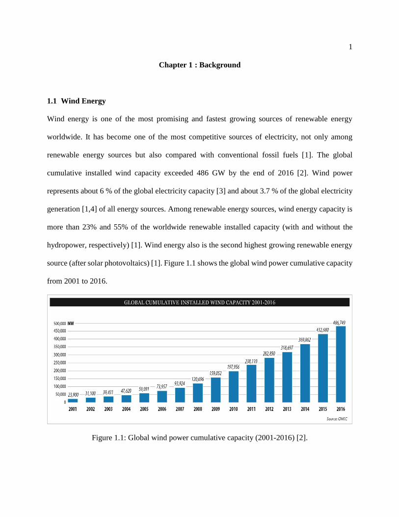
Wind energy is one of the most promising and fastest growing sources of renewable energy
worldwide. It has become one of the most competitive sources of electricity, not only among
renewable energy sources but also compared with conventional fossil fuels [1]. The global
cumulative installed wind capacity exceeded 486 GW by the end of 2016 [2]. Wind power
represents about 6 % of the global electricity capacity [3] and about 3.7 % of the global electricity
generation [1,4] of all energy sources. Among renewable energy sources, wind energy capacity is
more than 23% and 55% of the worldwide renewable installed capacity (with and without the
hydropower, respectively) [1]. Wind energy also is the second highest growing renewable energy
source (after solar photovoltaics) [1]. Figure 1.1 shows the global wind power cumulative capacity
from 2001 to 2016.
Figure 1.1: Global wind power cumulative capacity (2001-2016) [2].
2
1.2 Wind Turbines
Wind turbines convert a fraction of the wind’s kinetic energy into mechanical energy by direct
contact with its blades. Wind turbines are classified according to the direction of the axis of rotation
into two categories: horizontal-axis wind turbines and vertical-axis wind turbines. The former is
the most widely used and it is also the type considered in the proposed work, so reference will only
be made to “wind turbine(s)” or even “turbine(s)” throughout this thesis.
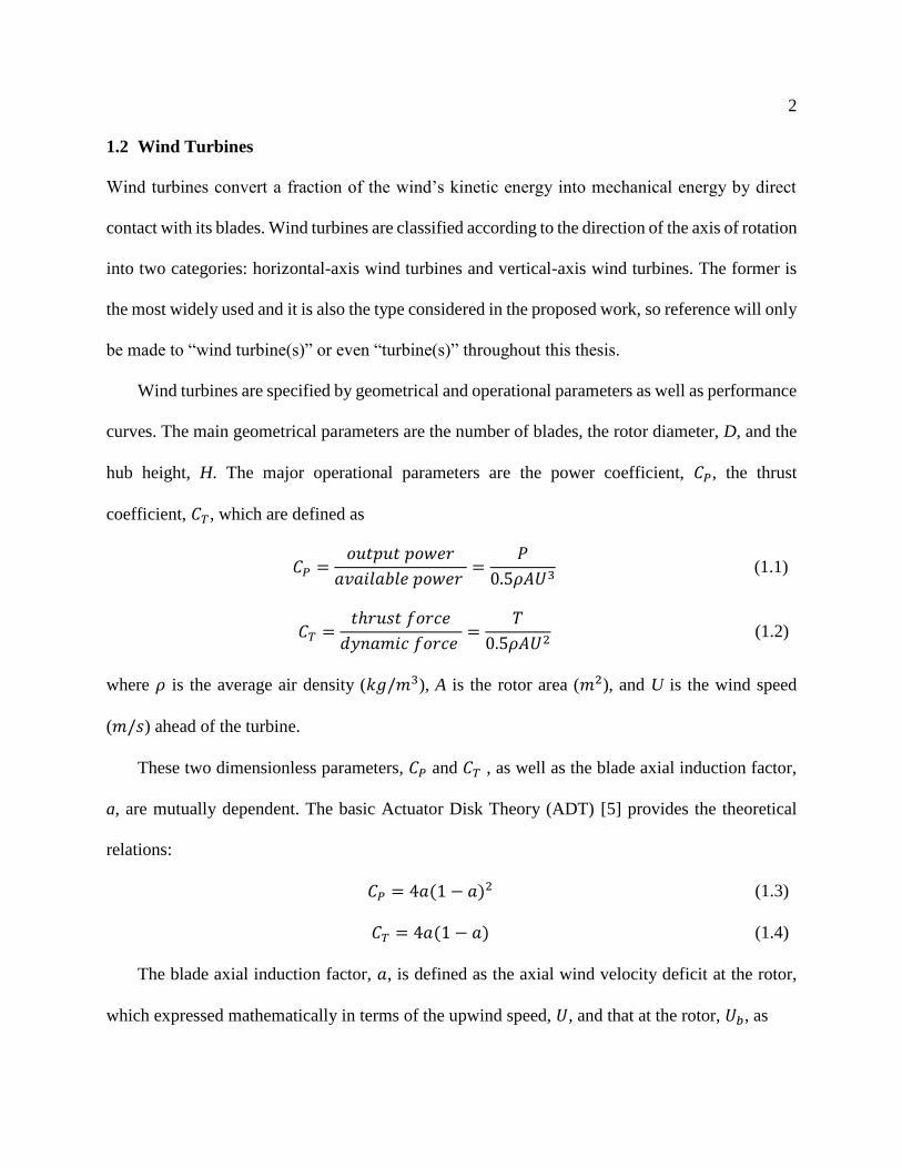
Wind turbines are specified by geometrical and operational parameters as well as performance
curves. The main geometrical parameters are the number of blades, the rotor diameter, D, and the
hub height, H. The major operational parameters are the power coefficient, 𝐶𝑃, the thrust
coefficient, 𝐶𝑇, which are defined as
𝐶𝑃 =𝑜𝑢𝑡𝑝𝑢𝑡 𝑝𝑜𝑤𝑒𝑟
𝑎𝑣𝑎𝑖𝑙𝑎𝑏𝑙𝑒 𝑝𝑜𝑤𝑒𝑟 =
𝑃
0.5𝜌𝐴𝑈3 (1.1)
𝐶𝑇 =𝑡ℎ𝑟𝑢𝑠𝑡 𝑓𝑜𝑟𝑐𝑒
𝑑𝑦𝑛𝑎𝑚𝑖𝑐 𝑓𝑜𝑟𝑐𝑒 =
𝑇
0.5𝜌𝐴𝑈2 (1.2)
where 𝜌 is the average air density (𝑘𝑔/𝑚3), A is the rotor area (𝑚2), and U is the wind speed
(𝑚/𝑠) ahead of the turbine.
These two dimensionless parameters, 𝐶𝑃 and 𝐶𝑇 , as well as the blade axial induction factor,
a, are mutually dependent. The basic Actuator Disk Theory (ADT) [5] provides the theoretical
relations:
𝐶𝑃 = 4𝑎(1 − 𝑎)2 (1.3)
𝐶𝑇 = 4𝑎(1 − 𝑎) (1.4)
The blade axial induction factor, 𝑎, is defined as the axial wind velocity deficit at the rotor,
which expressed mathematically in terms of the upwind speed, 𝑈, and that at the rotor, 𝑈𝑏, as

3
𝑎 =𝑈 − 𝑈𝑏
𝑈= 1 −
𝑈𝑏
𝑈 (1.5)
Figure 1.2 provides graphical representation for Equations (1.3) and (1.4), while Figure 1.3
shows the 𝐶𝑇-𝐶𝑃 curve according to the ADT analysis. Compared with commercial turbines,
Equations (1.3) and (1.4) overestimate 𝐶𝑃 for a particular 𝐶𝑇 (or underestimate 𝐶𝑇 for a particular
𝐶𝑃), as will be proven later in Chapter 4 and Chapter 5. ADT also indicates that no more than
16/27 of the kinetic energy that possessed by the air passing through a wind turbine rotor can be
converted into mechanical energy. This value is the maximum theoretical 𝐶𝑃 for a wind turbine
(known as the Betz- Joukowsky limit), when 𝑎 = 1/3 and 𝐶𝑇 = 8/9, as indicated in Figure 1.2
by the dashed vertical line.
Figure 1.2: CP and CT vs. a, according to the ADT equations.

4
Figure 1.3: CT - CP relation according to the ADT equations, up to the Betz-Joukowsky limit.
1.3 Wind Turbine Wake and Wake Modelling
By absorbing part of the wind’s kinetic energy, the wake behind the turbine rotor is characterized
by decreased wind speed and increased turbulence. The entrainment of the ambient (undisturbed)
air into the wake eventually leads to recovery so that far from a turbine the wind speed and
turbulence will have effectively returned to the undisturbed values. Wind turbine wake modelling
consists of characterizing the air flow (mainly the velocity and the turbulence level) downstream
of the rotor.
The wake behind a wind turbine has two main regimes: near wake, and far wake, e.g. [6,7].
The near wake, dominated by the tip and hub vortices, extends a few rotor diameters downstream,
where which the velocity deficit at the centerline reaches its maximum and the pressure equals the
free stream value [8]. On the other hand, the far wake is the region in which the actual rotor shape
is less important, but the focus lies on wake modeling, wake interference, turbulence modelling

5
and topographic effects, e.g. [6,9]. A third region may be considered between near and far wakes,
called transition, e.g. [8,9,10], or intermediate wake [11]. Figure 1.4 illustrates the flow structure
of a typical wind turbine wake.
Figure 1.4: Wind turbine wake structure [11].
Many wake models have been developed over the past five decades, extensive details can be
found in the review articles, e.g. [12,10,9,6,13]. For the present purposes, the aerodynamics of
wind turbines can be divided into two principal domains [14]:
I. The prediction of rotor performance (focusing only on the near wake).
II. The study of the wake (mainly the far wake) to evaluate the influence of wind turbines
in farms (which is the aspect of relevance to the current research).
The output power from a single wind turbine is limited (up to few MW), so wind turbines are
commonly installed in groups (wind farms) to increase the energy production. Any wind turbine

6
in a wind farm is affected by the wake(s) of the upwind turbine(s). Wake overlap (interference)
significantly affects the performance of the whole farm, especially downstream the first few
upwind rows, e.g. [10,15,16,17,18,19], after which their multiple wakes are merged [17].
1.4 Wind Farm Cost Breakdown
Although the wind is blowing freely, the conversion of wind’s kinetic energy into useful electrical
power is not free. The wind power Cost Of Energy (COE) significantly varies over time and
location and it also affected by the wind resources and the farm size, e.g. [20,21]. The major cost
of a wind power project is due to the initial capital cost, which represents more than 70 % and up
to 89 % of the total cost over the life span [22]. The operations and maintenance costs can be
represented globally as 11 - 30 % of the total cost over the life span [22] or annually as 1.5 - 3 %
of the initial capital cost [23].
The capital cost, in turn, is due to turbines, balance of the system, and financial costs [20].
The turbine cost represents the major part for onshore projects, while the balance of the system
cost is the major part of the offshore ones, as shown in Figure 1.5 and Figure 1.6, respectively.

7
Figure 1.5: Capital cost breakdown for a typical onshore wind power project [20].
Figure 1.6: Capital cost breakdown for a typical offshore wind power project [20].

8
1.5 The Wind Farm Layout Optimization Problem
As the wind power market expands, it faces increasing challenges, which can be classified in to
three main categories: technical, financial, and environmental. For example, to produce more
power from a wind farm, the number of turbines should increase and the turbines should be larger.
Besides, the turbines should be spaced further apart in order to reduce the wake interference. On
the other hand, larger turbines and/or larger wind farm area mean more cost (turbines, land, roads,
cables, etc.). Moreover, many restrictions have been put on wind farm installations because of their
environmental impact regarding noise, visual effects, flight paths, and even birds’ seasonal
immigration routes. All these factors increase the need for Wind Farm Layout Optimization
(WFLO), which investigates the ways to design wind farms so that the power is maximized while
the cost as well as the unwanted environmental impacts are minimized.
Any optimization problem, including the WFLO, consists of the four fields described in the
following sub-sections, e.g. [24,25]:
1.5.1 Design variables.
The design (or decision) variable is the parameter that needs to be determined (adjusted) in order
to achieve the optimum solution, e.g. [38,26,1]. The design variables must have upper and lower
limits within which the feasible solutions are obtained.
1.5.2 Constraints.
Optimization problems are usually subjected to restrictions (constraints), and hence not all
solutions are feasible. The upper and lower limits for the design variables are the simplest form of
constraints, and the integer constraint is another example, in which one (or more) of the design

9
variables, such as number of turbines, is (are) necessarily integer. Both upper and lower limits as
well as the integer constraints are linear, moreover, most the engineering optimization problems
are subjected to other constraints (linear and/or nonlinear) according the physics of the problem.
In the WFLO, the minimum turbine spacing is the most common nonlinear constraint on turbine
siting inside the farm is restricted.
1.5.3 Optimization technique.
The best optimization technique depends mainly on the nature of the problem as well as the
constraints. The present optimization problem is discrete, non-linear, non-convex, high-
dimensional, and mixed integer. Genetic algorithms (GAs) have been proven a powerful tool for
such complex problems, e.g. [27]. For this reason, GAs were implemented in most the WFLO
literature, although they are slow compared with the other optimization methods [26,1]. GAs are
computer programs that mimic the processes of biological evolution in order to solve problems
and to model evolutionary systems [28]. The solution is obtained by moving from one population
of chromosomes (feasible solutions) to a new population by using a kind of natural selection
(random search) together with the genetics-inspired operators of crossover, mutation, inversion,
etc. Each chromosome consists of a number of genes that are the possible values of the design
variables. The selection operator chooses those chromosomes in the population that will be
allowed to reproduce, and on average the fitter chromosomes produce more offspring than the less
fit ones [28]. A flowchart for GA used in the present work [29] is given in Figure 1.7.

10
Figure 1.7: Flowchart for Genetic Algorithm [29].
1.5.4 Optimization objectives.
An objective (fitness) function is simply the function that its value is to be optimized (maximized
or minimized), e.g. [26,1]. The objective in most of the WFLO literature is to maximize energy
production, minimize cost of energy, COE, maximize profit, or a combination of them [19].
1.6 Thesis Outline
An introduction to the topic of this thesis is given in this chapter. A literature review for the WFLO
problem followed by the motivation and research objectives are provided in Chapter 2. The rest of
the thesis is arranged as follows:

11
The selfish (individual) and the co-operative (collective) control alternatives for wind farms
are the topic of Chapter 3. The arrangement of Turbines In Line (TIL) is considered, as it gives the
maximum wake interference. The effect of wake recovery and topology are investigated.
The different efficiencies of commercial wind turbines relative to the ADT is introduced in
Chapter 4. The effect of the aerodynamic efficiency on the maximum power production is
investigated for both selfish and co-operative optimization strategies.
In Chapter 5, the power-COE trade-off is investigated. Selection among 61 commercial
turbines and common range of hub height variation are considered. The optimization is carried out
on two simple wind farm arrangements; 6 TIL and a 6-by-3 matrix of turbines.
Wind Farm Layout Upgrade Optimization (WFLUO) for existing farms is introduced in
Chapter 6. The famous large offshore wind farm (Horns Rev 1) is taken as case study. The power-
COE trade-off for both inside and outside upgrades are investigated. Commercial turbine selection
and turbine-specific hub height variation are employed. The cost model is modified and the GA is
improved by using Random Independent Multi-Population technique.
Finally, in Chapter 7, the chapters are concluded and the logical sequence of the different
chapters as one unit is explained.

12
1.7 References
1. REN21. 2016. Renewables 2016 Global Status Report (Paris: REN21 Secretariat). ISBN
978-3-9818107-0-7.
2. Global Wind Statistics 2016 (2017). Global Wind Energy Council GWEC.
3. http://www.tsp-data-portal.org/Breakdown-of-Electricity-Capacity-by-Energy-
Source#tspQvChart [last accessed: Dec. 2016].
4. http://www.gwec.net/global-figures/wind-in-numbers/ [last accessed: Dec. 2016].
5. Froude, R. E. (1889). On the part played in propulsion by difference in pressure.
Transaction of the Institute of Naval Architects, 30, pp. 390-423.
6. Sanderse, B. (2009). Aerodynamics of wind turbine wakes: literature review. ECN-e--09-
016.
7. Rathmann, O., Frandsen, S., Barthelmie, R. (2007). Wake modelling for intermediate and
large wind farms. Wind Energy Conference and Exhibition, Paper BL3.199.
8. Eecen, P.J., Bot, E.T.G., (2010). Improvements to the ECN wind farm optimisation
software "FarmFlow". ECN-M--10-055 , Presented at European Wind Energy Conference
and Exhibition, Warsaw, Poland.
9. Vermeer, L.J., Sørensen, J.N., Crespo, A. (2003). Wind turbine wake aerodynamics.
Progress in Aerospace Sciences, 39, pp. 467–510.
10. Crespo, A., Hernandez, J., Frandsen, S. (1999). Survey of modelling methods for wind
turbine wakes and wind farms. Wind Energy, 2, pp. 1-24.
11. Werle, M.J. (2008). A new analytical model for wind turbine wakes. FloDesign Inc.
Wilbraham MA, REPORT No. FD 200801.

13
12. Bossanyi, E. A., Maclean, C., Whittle, G. E., Dunn, P. D., Lipman, N. H., Musgrove, P. J.
(1980). The efficiency of wind turbine clusters. Proceedings of the 3rd International
Symposium on Wind Energy Systems, Lyngby, pp. 401-416.
13. Sanderse, B. (2011). Review of computational fluid dynamics for wind-turbine wake
aerodynamics. Wind Energy, 14, pp. 799–819.
14. El Kasmi, A., Masson, C. (2008). An extended 𝑘 − 𝜖 model for turbulent flow through
horizontal-axis wind turbines. Journal of Wind Engineering and Industrial Aerodynamics,
96, pp. 103–122.
15. Katic, I., Hojstrup, J., Jensen, N.O. (1986). A simple model for cluster efficiency. In
Proceedings of the European Wind Energy Association Conference and Exhibition, pp.
407–410.
16. Frandsen, S., Chacon, L., Crespo, A., Enevoldsen, P., Gomez-Elvira, R., Hernandez, J.,
Højstrup, J., Manuel, F., Thomsen, K., Sørensen, P. (1996). Measurements on and
modelling of offshore wind farms. Editor: Frandsen, S., Risø-R-903(EN), 100 p.
17. Frandsen, S., Barthelmie, R., Pryor, S., Rathmann, O., Larsen, S., Højstrup, J., Thøgersen,
M. L. (2006). Analytical modelling of wind speed deficit in large offshore wind farms.
Wind Energy, 9, pp. 39–53.
18. Kiani, A., Abdulrahman, M., Wood, D. (2014). Explicit solutions for simple models of
wind turbine interference. Wind Engineering, 38(2), pp. 167-180.
19. Tesauro, A., Réthoré, P-E, Larsen, G.C. (2012). State of the art of wind farm optimization.
Proceedings of European Wind Energy Conference & Exhibition, European Wind Energy
Association (EWEA 2012), Copenhagen, Denmark.

14
20. Mone, C., Hand, M., Bolinger, M., Rand, J., Heimiller, D., Ho, J. (2017). 2015 Cost of
Wind Energy Review. Technical Report, NREL/TP-6A20-66861, Revised May 2017.
[https://www.nrel.gov/docs/fy17osti/66861.pdf]
21. REN21. 2016. Renewables 2016 Global Status Report. (Paris: REN21 Secretariat). ISBN
978-3-9818107-0-7.
22. Schwabe, P., Lensink, S., Hand, M. (2011). IEA wind task 26: multi-national case study of
the financial cost of wind energy. Work Package 1, Final Report, NREL Report No. TP-
6A20-48155.
23. Manwell, J.F., McGowan, J.G., Rogers, A.L. (2009) Wind energy explained: Theory,
Design and Application, Second Edition, John Wiley & Sons, Ltd, Chichester, UK.
24. Boyd, S., Vandenberghe, L. (2009). Convex Optimization. Cambridge University Press,
New York.
25. Baldick, R. (2008). Applied Optimization, Formulation and algorithms for engineering
systems. Cambridge University Press, New York.
26. Samorani, M. (2010). The wind farm layout optimization problem. Technical Report,
Leeds School of Business, University of Colorado.
27. Kwong P., Zhang P.Y., Romero D.A., Moran J., Morgenroth M., Amon C.H. (2012). Wind
farm layout optimization considering energy generation and noise propagation. In
Proceedings of the ASME International Design Engineering Technical Conferences.
28. Melanie, M. (1999). An introduction to genetic algorithms. 5th Printing, MIT
Press, Cambridge, Massachusetts, USA.

15
29. Abdulrahman, M., Wood, D. (2017). Investigating the power-COE trade-off for wind farm
layout optimization considering commercial turbine selection and hub height variation.
Renewable Energy, 102 (B), pp. 267-516.

16
Chapter 2 : Literature Review
2.1 Introduction
As mentioned in section 1.5; the WFLO is the problem of designing wind farms so that the power
is maximized while the cost as well as the unwanted environmental impacts are minimized. The
interest in WFLO increased over the time as the installation of new large wind farm faces technical,
financial, and environmental challenges. WFLO is relatively new area of research; in 1994,
Mosetti et al. [1] studied this problem for the first time. They considered 10x10 square cells of
length 200 m, in which the 40 m rotor diameter turbines were possibly centered. Identical turbines
with constant thrust coefficient, 𝐶𝑇 = 0.88, as well as simple cubic power curve were considered.
Three cases were studied:
(1) uniform wind direction with constant wind speed,
(2) multi-directional wind with constant mean wind speed, and
(3) multi-directional wind with variable speeds.
The analytical Jensen’s wake model [2,3] was used to evaluate the wake behind the turbines.
A GA was implemented to maximize a combined objective function including the total power and
the inverse of the COE, using arbitrary weighting factors.
For the following decade, no significant contribution was added to WFLO. New aspects were
then added; either to the design variables, constraints, objective functions, and/or to the
optimization methodology.
Many researchers have analyzed the problem proposed by [1] in order to obtain better layouts
and/or reduce the computational time; either with some improvements to the GA, e.g. [4,5,6,7] or
by implementing other optimization strategies, e.g. [8,9,10,11,12].

17
2.2 Early Studies
Ozturk et al. [13] introduced a heuristic methodology to find layouts that maximize profit, which
is the product of the cost efficiency of the turbines and the total power output from the wind farm.
To evaluate their solution methodology, they constructed six test problems with different siting
area sizes.
Şişbot et al. [14] employed a multi-objective GA approach to optimize the layout for a
particular wind farm in order to maximize the power production while constraining the cost of
installed turbines.
Many other biologically-inspired algorithms have been also applied successfully for WFLO.
As examples: Particle Swarm Optimization [15,16], Ant Colony Optimization [17], Coral Reef
Optimization [18], and Viral Based Optimization [19].
Mixed Integer Programming (MIP) was proved to be a powerful tool in WFLO [20]. Many
Linear and Nonlinear MIP models have been developed and improved to find optimum layouts as
well as reducing the computational time, e.g. [21,22,23,20,24]. Monte Carlo Simulation [8,25] and
Simulated Annealing [26,27] were also successfully implemented for WFLO.
Landowner decisions and participation rates have been modeled as design variables and their
impact on WFLO has been investigated in series of publications by Chen and MacDonald
[28,7,29].
Recently, noise propagation has been added to the problem. Fagerfjäll [30] and Zhang et al.
[31] considered the noise level as a constraint in their optimization using Mixed Integer
Programming. Kwong et al. [32] considered noise level minimization as a second objective
function (beside the power production maximization) in their multi-objective optimization using
the Non-dominated Sorting Genetic Algorithm-II (NSGA-II) algorithm.

18
Very few studies have considered using different turbines and hub heights; these will be
reviewed in more detail in the next subsection.
2.3 Recent Studies
Herbert-Acero et al. [26] maximized the power production by a line of turbines in the wind
direction, using both Simulated Annealing and a Genetic Algorithm implemented in MATLAB.
This arrangement maximizes the power loss by interference. They used the technical data for
REpower, MD77 (rotor diameter, D = 77 m). Two values of hub height (H) were used, 50 m and
85 m, to reduce the effect of wake interference. The design parameters were the number of
turbines, their location, and the individual H while fixing the line length at 1,550 m. The results
showed that the placement of wind turbines with different heights could increase the power
generation in a straight line layout for a single wind speed and two opposite wind directions along
the line.
Chowdhury et al. [33,16] applied their Unrestricted Wind Farm Layout Optimization to
optimize the farm layout, simultaneously with the appropriate selection of turbines in terms of D
(while fixing H), in order to maximize the total power generation. Three different layout
optimization cases were considered:
(1) Wind farm with identical turbines,
(2) Wind farm with differing D, and
(3) Wind farm with identical turbines that can adapt to wind conditions (variable a
depending on the wind speed) as in the case of commercial turbines.
They found that an optimal combination of wind turbines with differing rotor diameters can
appreciably increase the farm power generation. They mentioned that a more practical wind farm

19
optimization requires the treatment of rotor diameters as discrete design variables, as there is only
a limited choice of commercial wind turbines.
Chowdhury et al. [34] significantly improved their method, enabling it to simultaneously
optimize the placement and the selection of turbines for commercial-scale wind farms to minimize
the COE. The number of turbines and the farm size were assumed to be fixed at the values for the
particular wind farm that they studied. They used the GE 1.5 xle-82.5 as the reference turbine and
normalized the manufacturer’s power curve with respect to the general specifications (rated power
(𝑃𝑟), cut-in and rated speeds, 𝑈𝑖𝑛 and 𝑈𝑟, respectively). This curve was assumed to hold for all
commercial turbines and scaled back to represent the power curve for any turbine (in the rated
power range from 0.6 to 3.6 MW) as long as the general specifications are defined, as shown in
Figure 2.1.
The results showed significant increase in energy production by simultaneous optimization of
the layout and the turbine selection compared with layout optimization alone. The optimum layout
contained turbines with rated power from 1.8 to 3 MW, with rotor diameters from 90 to 110 m,
and hub heights from 80 to 120 m.
Chen et al. [35] investigated the use of different H in a small wind farm layout optimization
using the GA function in MATLAB. They first conducted the layout optimization of a 500 m
square wind farm. Enercon E40-600kW turbines were used in the analysis with two values of hub
height, 50 and 78 m, and the minimum spacing was set as 100 m. Then a larger wind farm (2800
m x 1200 m) with larger wind turbine (GE 1.62-100) was analyzed to further examine the benefits
of using different hub heights (80 and 100 m) in more realistic conditions. The minimum spacing
was set as 400 m. Different cost models were used in the analysis, and results showed that different
hub height wind turbines can increase the power production and/or reduce the COE.

20
Figure 2.1: Normalized power curve for GE-1.5 xle-82.5, as developed by Chowdhury et al.
[34] and generalized for all turbines as long as the rated power, Pr, the rated speed, Ur, and the
cut-in speed, Uin, are defined.
Tong et al. [36], based on their previous work [16,37,38,34], have proposed a bi-level multi-
objective optimization framework considering the capacity factor and the land use as objective
functions. The capacity factor (CF) of a wind farm can be defined as the ratio of the actual (or
expected) output of the farm over a time period and the potential output if the farm was operating
at full nameplate capacity throughout that time period, e.g. [34]. Identical turbines were assumed,
and the design variables were the turbine locations, the land area, and the nameplate or rated
capacity. The model aimed to investigate the trade-off between the CF and the land use and its
effect on the optimum capacity.

21
2.4 Motivation and Research Objectives
By reviewing the WFLO literature, some deficiencies can be identified. The proposed work aims
to fill these gaps by adding the following dimensions to WFLO, which are considered also the
novelties of the presented work:
(1) The selection among a range of actual (commercial) turbines,
(2) The realistic evaluation of the turbine 𝐶𝑇, and hence the wake development, and
(3) Investigating the power-COE trade-off for WFLO, and
(4) Exploring the possibility and the feasibility for existing wind farms to be upgraded either
by extra turbines within the original farm area or outside that area.

22
2.5 References
1. Mosetti, G., Poloni, C., Diviacco, B. (1994). Optimization of wind turbine positioning in
large wind farms by means of a genetic algorithm. Journal of Wind Engineering and
Industrial Aerodynamics, 51, pp. 105-116.
2. Jensen, N.O. (1983). A note on wind generator interaction. Risø-M-2411, Risø National
Laboratory.
3. Katic, I., Hojstrup, J., Jensen, N.O. (1986). A simple model for cluster efficiency. In
Proceedings of the European Wind Energy Association Conference and Exhibition, pp.
407-410.
4. Grady, S.A., Hussaini, M.Y., Abdullah, M.M. (2005). Placement of wind turbines using
genetic algorithms. Renewable Energy. 30(2), pp. 259-270.
5. Hou-Sheng, H. (2007). Distributed genetic algorithm for optimization of wind farm annual
profits. International Conference on Intelligent Systems Applications to Power Systems,
ISAP 2007, Kaohsiung, Taiwan.
6. Emami, A., Noghreh, P. (2010). New approach on optimization in placement of wind
turbines within wind farm by genetic algorithms. Renewable Energy, 35, pp. 1559-1564.
7. Chen, L., MacDonald, E. (2012). Considering landowner participation in wind farm layout
optimization. Journal of Mechanical Design, 134, 084506-1:6.
8. Marmidis, G., Lazarou, S., Pyrgioti, E. (2008). Optimal placement of wind turbines in a
wind park using monte carlo simulation. Renewable Energy, 33, pp. 1455–1460.
9. González, J.S., Gonzalez Rodriguez, A.G., Mora, J.C., Santos, J.R., Payan, M.B. (2010).
Optimization of wind farm turbines layout using an evolutive algorithm. Renewable
Energy, 35(8), pp. 1671-1681.

23
10. Ituarte-Villarreal, C.M., Espiritu, J.F. (2011). Wind turbine placement in a wind farm using
a viral based optimization algorithm, Procedia Computer Science, 6, pp. 469–474.
11. Turner, S.D.O., Romero, D.A., Zhang, P.Y., Amon, C.H., Chan, T.C.Y. (2014). A new
mathematical programming approach to optimize wind farm layouts. Renewable Energy
63(c), pp. 674–680.
12. Zhang, P.Y., Romero, D.A., Beck, J.C., Amon, C.H. (2014). Solving wind farm layout
optimization with mixed integer programming and constraint programming. EURO Journal
on Computational Optimization, 2(3), pp. 195-219.
13. Ozturk, U.A, Norman B.A. (2004). Heuristic methods for wind energy conversion system
positioning. Electric Power Systems Research, 70, pp. 179–185.
14. Şişbot, S., Turgut, Ö., Tunç1and, M., Çamdalı, Ü. (2010). Optimal positioning of wind
turbines on gökçeada using multi-objective genetic algorithm. Wind Energy, 13(4), pp.
297–306.
15. Wan, C., Wang, J., Yang, G., Zhang, X. (2010). Optimal micro-siting of wind farms by
particle swarm optimization. In: Advances In Swarm Intelligence, Berlin, Heidelberg, pp.
198-205.
16. Chowdhury, S., Zhang, J., Messac, A., Castillo, L. (2012). Unrestricted wind farm layout
optimization (UWFLO): Investigating key factors influencing the maximum power
generation. Renewable Energy, 38(1), pp. 16–30.
17. Eroğlu, Y., Seçkiner S.U. (2012). Design of wind farm layout using ant colony algorithm.
Renewable Energy, 44, pp. 53-62.

24
18. Salcedo-Sanz, S., Gallo-Marazuela, D., Pastor-Sánchez, A., Carro-Calvo, L., Portilla-
Figueras, A., Prieto L. (2014). Offshore wind farm design with the coral reefs optimization
algorithm. Renewable Energy, 63, pp. 109-115.
19. Ituarte-Villarreal, C.M., Espiritu, J.F. (2011). Wind turbine placement in a wind farm using
a viral based optimization algorithm. Procedia Computer Science, 6, pp. 469–474.
20. Donovan, S. (2006). An improved mixed integer programming model for wind farm layout
optimization. In: Proceedings of the 41st annual conference of the Operations Research
Society, Wellington.
21. Turner, S.D.O., Romero, D.A., Zhang, P.Y., Amon, C.H., Chan, T.C.Y. (2014). A new
mathematical programming approach to optimize wind farm layouts. Renewable Energy
63(c), pp. 674–680.
22. Zhang, P.Y., Romero, D.A., Beck, J.C., Amon, C.H. (2014). Solving wind farm layout
optimization with mixed integer programming and constraint programming. EURO Journal
on Computational Optimization, 2(3), pp. 195-219.
23. Donovan, S. (2005). Wind farm optimization, In: Proceedings of the 40th annual conference
of the Operations Research Society, Wellington.
24. Archer, R., Nates, G., Donovan, S., Waterer, H. (2011). Wind turbine interference in a
wind farm layout optimization mixed integer linear programming model. Wind
Engineering, 35, pp. 165-178.
25. Brusca, S., Lanzafame, R., Messina M. (2014). Wind turbine placement optimization by
means of the monte carlo simulation method. Modelling and Simulation in Engineering
Volume 2014.

25
26. Herbert-Acero, J-F., Franco-Acevedo, J-R., Valenzuela-Rendon, M., Probst-Oleszewski,
O. (2009). Linear wind farm layout optimization through computational intelligence.
Proceedings of 8th Mexican International Conference on Artificial Intelligence, pp. 692–
703.
27. Rivas, R.A., Clausen, J., Hansen, K.S., Jensen, L.E. (2009). Solving the turbine positioning
problem for large offshore wind farms by simulated annealing. Wind Engineering, 33, pp.
287–297.
28. Chen, L., MacDonald, E. (2011). A New Model for Wind Farm Layout Optimization with
Landowner Decisions, In: Proceedings of the ASME 2011 International Design
Engineering Technical Conferences and Computers and Information in Engineering
Conference, pp. 303-314.
29. Chen, L., MacDonald, E. (2014). A system-level cost-of-energy wind farm layout
optimization with landowner modeling. Energy Conversion and Management, 77, pp. 484-
494.
30. Fagerfjäll, P. (2010). Optimizing wind farm layout: More bang for the buck using mixed
integer linear programming. MSc Thesis, Chalmers University of Technology and
Gothenburg University.
31. Zhang, P.Y., Romero, D.A., Beck, J.C., Amon, C.H. (2014). Solving wind farm layout
optimization with mixed integer programming and constraint programming. EURO Journal
on Computational Optimization, 2(3), pp. 195-219.
32. Kwong P., Zhang P.Y., Romero D.A., Moran J., Morgenroth M., Amon C.H. (2012). Wind
farm layout optimization considering energy generation and noise propagation. In
Proceedings of the ASME International Design Engineering Technical Conferences.

26
33. Chowdhury, S., Messac, A., Zhang, J., Castillo, L., Lebron, J. (2010). Optimizing the
unrestricted placement of turbines of differing rotor diameters in a wind farm for maximum
power generation. ASME 2010 International Design Engineering Technical Conferences
and Computers and Information in Engineering Conference, Paper No. DETC2010-29129,
pp. 775-790.
34. Chowdhury, S., Zhang, J., Messac, A., Castillo, L. (2013). Optimizing the arrangement and
the selection of turbines for wind farms subject to varying wind conditions. Renewable
Energy, 52, pp. 273-282.
35. Chen, Y., Li, H., Jin, K., Song, Q. (2013). Wind farm layout optimization using genetic
algorithm with different hub height wind turbines. Energy Conversion and Management,
70, pp. 56–65.
36. Tong, W., Chowdhury, S., Mehmani, A. Messac, A. (2013). Multi-objective wind farm
design: Exploring the trade-off between capacity factor and land use. 10th World Congress
on Structural and Multidisciplinary Optimization, Orlando, Florida.
37. Chowdhury, S., Tong, W., Messac, A., Zhang, J. (2012). A mixed-discrete particle swarm
optimization algorithm with explicit diversity-preservation. Structural and
Multidisciplinary Optimization, 47(3), pp. 367-388.
38. Chowdhury, S., Zhang, J., Messac, A., Castillo, L. (2012). Characterizing the influence of
land area and nameplate capacity on the optimal wind farm performance. In ASME 2012
6th International Conference on Energy Sustainability, San Diego, pp. 1349-1359.

27
Chapter 3 : Explicit Solutions for Simple Models of Wind Turbine Interference
Abstract
Wind turbine interference - the reduction in output power of a turbine downwind of any others - is
a major problem for wind farm optimization and control. With interference, it is well-known for
specific cases that co-operative optimization of power output yields more power than does the
selfish optimization of individual turbines. This paper develops explicit solutions for simple
models of interference for the general case of any number of turbines in line with the wind. For
the simplest case of no wake recovery, analytical solutions for co-operative and selfish
optimization are derived. They show that co-operative optimization nearly always yields more
power and never yields less. Adding a simple form of wake recovery for equally spaced turbines
precludes analytical solutions, but numerical solutions are developed to find the power to any
required level of accuracy. Again, co-operative optimization is superior in nearly all cases. These
simple solutions should be useful for demonstrating the importance of interference and for testing
methods for optimizing wind farm layout and operation. It is shown that the maximum benefit
from co-operative operation occurs at turbine spacing comparable to that commonly used in wind
farms. The analysis is then extended to include topographical effects modeled as changes in wind
speed along the line. Explicit solutions are obtained for two turbines in line. Co-operative
optimization remains the best strategy. In particular, when the wind speed increases, it quickly
becomes optimal to shut down the first turbine.

28
3.1 Introduction
Wind energy is usually harvested by wind farms that consist of multiple wind turbines located in
a particular layout over a substantial stretch of land (onshore) or water (offshore). It has been
shown in the literature (see [1,2,3,4,5]) that the total power extracted by a wind farm is often
significantly less than the simple product of the power extracted by a stand-alone turbine and the
number of turbines in the farm. The loss in energy is due mainly to interference on any downwind
turbines due to the wake of the upwind machines [6].
Given the primary effect of the wake in the reduction of the wind farm power, an analytical
wake model is an important tool to study and particularly mitigate interference. The Park wake
model, originally developed by Jensen [7] and later completed by Katic et al. [8], is one of the
most popular analytical wake models used in wind farm modeling. The modified Park wake model
and the Eddy Viscosity wake model are other standard wake models [6]. The Park model includes
wake recovery, the entrainment of the external flow into the turbine wake to re-energize it.
Recently, Hancock [9] analyzed turbines in a line by an extension of the one-dimensional analysis
using conservation of mass, momentum, and energy, that leads to the Betz-Joukowsky limit for a
single turbine (1). Hancock extended his model to include a simple form of wake recovery that we
will also use in this paper.
The loss of output power due to interference depends primarily on the geometric arrangement
of multiple wind turbines in relation to the important wind directions. Hence, an optimal layout of
turbines that ensures maximum output power is expected to improve the economics of a wind farm
project (see [2,3,4]).
(1) Okulov & van Kuik [10] recently argued that the commonly-termed Betz limit should be attributed to Joukowsky as well.

29
Another factor that plays an important role in increasing wind farm power in the presence of
interference is the co-ordination of the control of power output among the turbines in the wind
farm. There should be a close interaction between layout design and operational control which is
not addressed in this paper. We assume that the wind farm layout is given and the goal of this
paper is to provide a collective adjustment of the power output of multiple wind turbines in line to
maximize the total output power. Following Hancock [9], we consider the extreme case of the
interaction within a farm that occurs when turbines form a straight line in the wind direction, as
this minimizes the energy available to the downwind turbines.
Studies of control methodologies by Herbert-Accro et al. [11], Madjidian & Rantzer [12], and
Marden et al. [13] show that co-operative optimization produces more power than does selfish
optimization of the individual turbines. This paper considers co-operative and selfish optimization
for simple wake models. It starts with Hancock’s basic model to develop a closed form
maximization of the power output from N identical turbines in line with no wake recovery.
Hancock’s second model with wake recovery reduces to the first as a special case but cannot
generally be solved in closed form. However, we describe an iterative solution which can be made
arbitrarily accurate for any 𝑁. Power optimization is done for two cases. In the first, the 𝑁 turbines
are individually maximized which is an 𝑁-dimensional problem. In the second case, a simpler one-
dimensional optimization of the collective or co-operative power is considered. We demonstrate
explicitly and numerically that the maximum co-operative power is never less than the sum of the
maximum individual powers, and in many cases, it is considerably higher. For simplicity, we
assume that the turbines are equi-spaced.
Finally, we consider some effects of topography, modeled as a change in wind speed along
the line of turbines. Because this change is likely to be different for each turbine, we do not attempt

30
to solve the general problem. Analytic solutions are developed for selfish and co-operative
optimization of two turbines in line with wind speed changes. Again, co-operative optimization is
superior. In particular, we find a special case of co-operative optimization, “sacrificial”
optimization in which power output is maximized if the first turbine is shut down when the wind
speed increases from the first to second. Sacrificial optimization is valid even for small increases
in the wind speed from the first to second turbine.
The main contributions of this paper are:
(1) A simple analysis which shows the advantage of co-operative turbine operation when there
is no wake interference with and without topographical effects.
(2) A more sophisticated analysis that includes a form of wake recovery. The equations can
be solved iteratively to arbitrary accuracy. Co-operative optimization is shown to be most
beneficial at turbine spacing typical of modern wind farms.
(3) In all cases, the co-operative maximum power was shown to be greater than the sum of
the maximum individual powers. This result is proved for the first simple model for an
arbitrary number of turbines, and demonstrated numerically for the second model. The
superiority of co-operative optimization is established analytically for wake recovery for
two turbines in line, with wind speed changes between them.
This paper is organized as follows. In the next section, we derive the equation for the power
output of N turbines in line without wake recovery. This is largely a restatement of the analysis of
Hancock [9]. In Section 3.1, we analyze the case where each turbine maximizes its power
extraction. Then in Section 3.2, we will present the results for maximization of the overall output.
A simplified form of the Park model which modifies the induction factor of the wake is presented

31
in Section 3.4. Following this, numerical simulations are provided in Section 3.5. Topographical
effects are considered in Section 3.6. Concluding remarks are made in Section 3.7.
3.2 The Basic Model of Turbines In Line
Denote the induction factor in the wake of the 𝑛𝑡ℎ turbine as 𝑎𝑛, the wind speed by 𝑈 and turbine
area by 𝐴. 𝑎𝑛 is defined relative to 𝑈 and there is no compounding of 𝑎𝑛 for the downwind turbines.
We assume that the 𝑁 turbines in line are identical. From Hancock’s formulation of the momentum
equation, the thrust of the 𝑛𝑡ℎ turbine, 𝑇𝑛, in the presence of the wake of the (𝑛 − 1)𝑡ℎ turbine can
be written as
𝑇𝑛 = 𝜌𝑈(1 − 𝑎𝑏,𝑛)𝐴[𝑈(1 − 𝑎𝑛−1) − 𝑈(1 − 𝑎𝑛)] (3.1)
or
𝑇𝑛 = 𝜌𝑈2𝐴(1 − 𝑎𝑏,𝑛)(𝑎𝑛 − 𝑎𝑛−1) (3.2)
where 𝑎𝑏,𝑛 is the induction factor at the blades of turbine n. The pressure difference across the
rotor can be found using Bernoulli’s equation for the upwind and downwind flow for each turbine:
𝑃+ − 𝑃− = 1
2𝜌𝑈2(1 − 𝑎𝑛−1)2 −
1
2𝜌𝑈2(1 − 𝑎𝑛)2 (3.3)
From Equation (3.3), the thrust of turbine 𝑛 is
𝑇𝑛 = (𝑃+ − 𝑃−)𝐴 = 1
2𝜌𝑈2𝐴[(1 − 𝑎𝑛−1)2 − (1 − 𝑎𝑛)2]
=1
2𝜌𝑈2𝐴(𝑎𝑛 − 𝑎𝑛−1)(2 − 𝑎𝑛 − 𝑎𝑛−1) (3.4)
Comparing Equation (3.2) with Equation (3.4), it follows that
𝑎𝑏,𝑛 = (𝑎𝑛 + 𝑎𝑛−1)
2 (3.5)

32
From the energy equation, the power output of turbine 𝑛 is
𝑃 = 1
2𝜌𝑈3𝐴(1 − 𝑎𝑏,𝑛)[(1 − 𝑎𝑛−1)2 − (1 − 𝑎𝑛)2] (3.6)
Defining 𝐶𝑃,𝑛 as the power coefficient of the 𝑛𝑡ℎ turbine in the normal manner allows Equation
(3.6) to be combined with Equation (3.5) to give
𝐶𝑃,𝑛 =𝑃
12 𝜌𝑈3𝐴
= 1
2(𝑎𝑛 − 𝑎𝑛−1)(2 − 𝑎𝑛 − 𝑎𝑛−1)2 (3.7)
Now consider two different cases: in the first case designated as “selfish” optimization, each
individual 𝐶𝑃,𝑛 is maximized. The second case of “co-operative” optimization, maximizes
∑ 𝐶𝑃,𝑛𝑁𝑛=1 . As with the common derivation of the Betz–Joukowsky equation, optimization is based
on selecting the value of 𝑎𝑛 to maximize the power.
3.3 Optimization of the Power Output
3.3.1 Selfish optimization.
To maximize the power for each individual turbine from Equation (3.7), we set
𝜕𝐶𝑃,𝑛
𝜕𝑎𝑛=
1
2(3𝑎𝑛 − 𝑎𝑛−1 − 2)(𝑎𝑛 + 𝑎𝑛−1 − 2) = 0 (3.8)
Since 𝑎𝑛 , 𝑎𝑛−1 < 1,
3𝑎𝑛 = 𝑎𝑛−1 + 2 (3.9)
Given 𝑎0 = 0, it follows that
𝑎1 =2
3 (3.10)
which is the Betz-Joukowsky value. By extension to the downwind turbines, we obtain

33
𝑎2 =1
3(
2
3+ 2) =
2
32+
2
3 𝑎𝑛𝑑 𝑎3 =
1
3[1
3(
2
3+ 2)] =
2
33+
2
32+
2
3 (3.11)
Generalizing Equation (3.11) gives 𝑎𝑛 as
𝑎𝑛 = 2 ∑1
3𝑖
𝑛
𝑖=1
= 1 − 3−𝑛 (3.12)
It is easy to interpret Equation (3.12) as showing that each turbine operates at the Betz–Joukowsky
limit with the “wind” speed equal to the wake velocity of the immediately upwind turbine. For 𝑛
sufficiently large, 𝑎𝑛 → 1. Using Equation (3.12), the sum of the power coefficients can be
calculated as
∑ 𝐶𝑃,𝑛
𝑁
𝑛=1
=1
2∑(2 − 𝑎𝑛 − 𝑎𝑛−1)2
𝑁
𝑛=1
(𝑎𝑛 − 𝑎𝑛−1)
=1
2∑(3−𝑛 + 3−𝑛+1)2
𝑁
𝑛=1
(3−𝑛 + 3−𝑛+1) (3.13)
Summing Equation (3.13), we obtain
∑ 𝐶𝑃,𝑛
𝑁
𝑛=1
=8
13(1 −
1
33𝑁) →
8
13 𝑎𝑠 𝑁 → ∞ (3.14)
Equation (3.14) gives the maximum power obtainable from 𝑁 turbines in line if each maximizes
its power. For 𝑁 = 1, Equation (3.14) reduces to the Betz-Joukowsky limit which is only 3.8 %
less than the maximum possible power coefficient, 8/13, for an infinite line of turbines.
3.3.2 Co-operative optimization.
From Equation (3.7), the contribution to the sum of the power coefficients from terms involving
𝑎𝑛 is

34
∆𝑛= 𝐶𝑃,𝑛 + 𝐶𝑃,𝑛+1, 𝑓𝑜𝑟 1 < 𝑛 < 𝑁
=1
2[(2 − 𝑎𝑛 − 𝑎𝑛−1)2(𝑎𝑛 − 𝑎𝑛−1) + (2 − 𝑎𝑛+1 − 𝑎𝑛)2(𝑎𝑛+1 − 𝑎𝑛)] (3.15)
To find the 𝑎𝑛 that maximizes the sum of the power from the turbines up to 𝑁 − 1, we set
𝜕∆𝑛
𝜕𝑎𝑛= 0, 𝑜𝑟
1
2[(3𝑎𝑛 − 𝑎𝑛−1 − 2)(𝑎𝑛 + 𝑎𝑛−1 − 2) + (3𝑎𝑛+1 − 𝑎𝑛 − 2)(𝑎𝑛+1 + 𝑎𝑛 − 2)] = 0 (3.16)
It follows that
𝑎𝑛 =(𝑎𝑛−1 + 𝑎𝑛+1)
2, 𝑓𝑜𝑟 1 < 𝑛 < 𝑁 (3.17)
Obviously, Equation (3.17) does not apply to the last turbine which must be considered separately.
Given that 𝑎0 = 0, it follows that 𝑎2 = 2𝑎1, and 𝑎3 = 3𝑎1. It is easy to use induction to establish
the general result that
𝑎𝑛 = 𝑛𝑎1, 𝑓𝑜𝑟 1 < 𝑛 < 𝑁 (3.18)
The 𝑁𝑡ℎ turbine must operate according to Equation (3.9) with 𝑛 = 𝑁. Substituting Equation
(3.18) into Equation (3.7) and evaluating the sum gives
∑ 𝐶𝑃,𝑛 = 𝑎1
2∑(2 − 2𝑛𝑎1 + 𝑎1)2 +
16
27[1 − (𝑁 − 1)𝑎1]3
𝑁−1
𝑛=1
𝑁
𝑛=1
=𝑁 − 1
6[12𝑎1 − 12(𝑁 − 1)𝑎1
2 + 4𝑎13(𝑁 − 1)2] +
16
27[1 − (𝑁 − 1)𝑎1]3 (3.19)
Equation (3.19) shows the power output of all 𝑁 turbines now depends only on 𝑎1. The maximum
total power occurs when
𝜕 ∑ 𝐶𝑃,𝑛𝑁𝑛=1
𝜕𝑎𝑛=
𝑁
18[4 − 8𝑁𝑎1 − (4𝑁2 − 9)𝑎1
2] = 0 (3.20)

35
Solving Equation (3.20) yields
𝑎1 = 1/ (𝑁 +1
2) (3.21)
When 𝑁 = 1, Equation (3.21) gives 𝑎1 = 2/3 and when 𝑁 tends to infinity, 𝑎1 → 1/𝑁. Using
Equation (3.21), the maximum total power for 𝑁 turbines is
∑ 𝐶𝑃,𝑛
𝑁
𝑛=1
=2𝑁(𝑁 + 1)
3 (𝑁 +12
)2 →
2
3 𝑎𝑠 𝑁 → ∞ (3.22)
The asymptotic result is a small increment (12.5%) above the Betz-Joukowsky limit for a
single turbine. Nevertheless, co-operative optimization always gives the same or more power than
selfish optimization. Let 𝛿(𝑁) denote the difference in the sum of power outputs between N co-
operative turbines and N selfish turbines. Equations (3.14) and (3.22) give
𝛿(𝑁) = 8
39(31−𝑁 +
𝑁2 + 𝑁 − 3
(1 − 2𝑁)2) (3.23)
𝛿(1) = 0 obviously, but 𝛿(𝑁) > 0 for any 𝑁 > 1.
3.4 Optimization with Wake Recovery
We now use a simplified form of the Park model which modifies the induction factor of the wake
of the (𝑛– 1)𝑡ℎ turbine before that wake reaches the 𝑛𝑡ℎ turbine in an equi-spaced line. The upwind
induction factor of the 𝑛𝑡ℎ turbine is 𝑎𝑛–1′ = 𝑏𝑎𝑛–1, where, as before, 𝑎𝑛–1 is the wake induction
factor for the (𝑛– 1)𝑡ℎ turbine, and 𝑏 ≤ 1. The factor 𝑏 is identical to 𝑓 used by Hancock [9]. It
allows for some wake recovery by entrainment of external air at higher wind speed. Thus,
𝐶𝑃,𝑛 =1
2(2 − 𝑎𝑛 − 𝑏𝑎𝑛−1)2(𝑎𝑛 − 𝑏𝑎𝑛−1) (3.24)
We now extend the results in Sections 3.3.1 and 3.3.2 to include 𝑏.

36
3.4.1 Selfish optimization with wake recovery.
Modifying Equation (3.8), using the wake recovery model in Equation (3.24), we have
𝜕𝐶𝑃,𝑛
𝜕𝑎𝑛=
1
2(3𝑎𝑛 − 𝑏𝑎𝑛−1 − 2)2(𝑎𝑛 + 𝑏𝑎𝑛−1 − 2) = 0
Since b ≤ 1, the second term can never be zero and therefore
𝑎𝑛 =(𝑏𝑎𝑛−1 + 2)
3, 𝑓𝑜𝑟 1 ≤ 𝑛 ≤ 𝑁 (3.25)
Thus for 𝑏 ≤ 1,
𝑎0 = 0, 𝑎1 =2
3 , 𝑎2 =
1
3[2𝑏
3+ 2] =
2𝑏
32+
2
3
and, in general,
𝑎𝑛 = 2 ∑𝑏𝑖−1
3𝑖=
2 − 2 (𝑏3)
𝑛
3 − 𝑏
𝑛
𝑖=1
(3.26)
Substituting Equation (3.26) in Equation (3.24), we obtain
∑ 𝐶𝑃,𝑛 = 2 ∑ [2 − 2𝑏 + 4 (
𝑏3)
𝑛
3 − 𝑏]
3𝑁
𝑛=1
𝑁
𝑛=1
(3.27)
When the turbines are far enough apart, 𝑏 → 0. In this case, Equation (3.27) implies that
∑ 𝐶𝑃,𝑛
𝑁
𝑛=1
=16
27𝑁 (3.28)
which shows that each turbine operates at the Betz-Joukowsky limit. When 𝑏 = 1, we recover the
simple model result, Equation (3.14). It should be noted that from Equation (3.27) does not have
a compact summation as did Equation (3.14). It is probably better to evaluate the sum directly for
each 𝑁.

37
3.4.2 Co-operative optimization with wake recovery.
The contribution to the overall power coefficient from the (𝑛 − 1)𝑡ℎ and 𝑛𝑡ℎ turbines denoted in
Equation (3.15) becomes
∆𝑛= (2 − 𝑎𝑛 − 𝑏𝑎𝑛−1)2(𝑎𝑛 − 𝑏𝑎𝑛−1) + (2 − 𝑎𝑛+1 − 𝑏𝑎𝑛)2(𝑎𝑛+1 − 𝑏𝑎𝑛)
As in Section 3.3.2, the maximum power occurs when
𝜕∆𝑛
𝜕𝑎𝑛= 4 + 𝑏(𝑎𝑛+1
2 − 𝑏𝑎𝑛−12 − 4) − 3(𝑏3 − 1)𝑎𝑛
2 +
+2𝑎𝑛[𝑏(𝑎𝑛−1 − 𝑏𝑎𝑛+1 + 4𝑏) − 4] = 0
(3.29)
Rewriting Equation
(3.29) to make 𝑎𝑛 the subject gives
𝑎𝑛̅̅ ̅ =4 + 𝑏(𝑎𝑛+1
2 − 𝑏𝑎𝑛−12 − 4) − 3(𝑏3 − 1)𝑎𝑛
2
2[4 − 𝑏(𝑎𝑛−1 − 𝑏𝑎𝑛+1 + 4𝑏)] (3.30)
where 𝑎𝑛̅̅ ̅ indicates that the equation can be used to iterate for 𝑎𝑛 as solving the quadratic equations
for every n would also have to be done iteratively. Again 𝑎0 = 0 independent of 𝑏.
The form of Equation (3.30) suggests an analytic solution is possible only when 𝑏 = 1 or 0.
When 𝑏 = 0, Equation (3.30) does not require iteration and 𝑎𝑛 = 2/3 from Equation (3.10). When
𝑏 = 1, Equation (3.30) reduces to Equation (3.17), again without iteration. For the 𝑁𝑡ℎ turbine,
𝑎𝑁+1 = 0 so 𝑎𝑁 is given by Equation (3.25) and the power output of the last turbine is
𝐶𝑃,𝑁 = (2 − 𝑎𝑁 − 𝑏𝑎𝑁−1)2(𝑎𝑛 − 𝑏𝑎𝑛−1) (3.31)
3.5 Optimization Examples and Numerical Simulation
Figure 3.1 and Figure 3.2 compare the maximum co-operative power output to the individually
optimized power. As 𝑏 → 0, the turbines become far enough apart to operate independently and

38
the co-operative and individual optimizations yield the same total power. For all other 𝑏, co-
operative optimization produces more power, with the biggest improvement around 𝑏 = 0.7. In
this version of the Park model we can approximate
𝑏 = (1 + 2𝑘𝑥)−2 (3.32)
where the empirical factor 𝑘 has the value of 0.075 in the well-known software WAsP, and 𝑥 is
the distance between the turbines of diameter 𝐷. Thus, 𝑏 = 0.4 corresponds to turbines spaced
four diameters apart, which is about the minimum distance used in practice.
Figure 3.1: Total power output from co-operative (symbols) and individual (solid lines)
optimization as a function of 𝑏. The number of turbines in the line is indicated on the Figure.

39
Figure 3.2: Ratio of total power output from co-operative optimization to individual
optimization. Lines for visual aid only. The number of turbines in the line is indicated on the
Figure.
The assumption of constant 𝑏 is an approximation to the Park model because no account is
taken of the interaction of successive wakes when 𝑁 > 2.
Figure 3.3 shows the induction factors for selfish (𝑁 = 12) and co-operative optimization for
𝑁 = 3, 6, 9, 𝑎𝑛𝑑 12. The difference in operation between the two types of optimization is much
more obvious in 𝑎𝑛 than in the power output. Figure 3.4 shows the variation in 𝑎𝑛 with 𝑛 for 𝑁 =
5 and varying 𝑏 for co-operative optimization. For the extreme case of 𝑏 = 0 (𝑎𝑛 = 2/3) all
turbines operate at the Betz-Joukowsky limit. With no wake recovery, 𝑏 = 1 and 𝑎𝑛 = 𝑛
𝑁+0.5 from
Equation (3.18) and Equation (3.21)).

40
Figure 3.3: Wake induction factors for 𝑏 = 0.5. Individual optimization for 𝑁 = 12, shown by
diamonds. Other results for co-operative optimization for 𝑁 indicated by last symbol.
Figure 3.4: Induction factors for co-operative optimization for 𝑁 = 5 as a function of 𝑏.
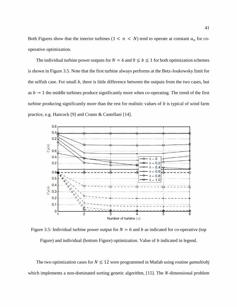
41
Both Figures show that the interior turbines (1 < 𝑛 < 𝑁) tend to operate at constant 𝑎𝑛 for co-
operative optimization.
The individual turbine power outputs for 𝑁 = 6 and 0 ≤ 𝑏 ≤ 1 for both optimization schemes
is shown in Figure 3.5. Note that the first turbine always performs at the Betz-Joukowsky limit for
the selfish case. For small 𝑏, there is little difference between the outputs from the two cases, but
as 𝑏 → 1 the middle turbines produce significantly more when co-operating. The trend of the first
turbine producing significantly more than the rest for realistic values of 𝑏 is typical of wind farm
practice, e.g. Hancock [9] and Crasto & Castellani [14].
Figure 3.5: Individual turbine power output for 𝑁 = 6 and 𝑏 as indicated for co-operative (top
Figure) and individual (bottom Figure) optimization. Value of 𝑏 indicated in legend.
The two optimization cases for 𝑁 ≤ 12 were programmed in Matlab using routine gamultiobj
which implements a non-dominated sorting genetic algorithm, [15]. The 𝑁-dimensional problem

42
of Case 1 was always evaluated with larger error than Case 2. For the latter, gamultiobj with the
default parameters and a population size of 100 gave results so close to those from the present
theory, that there would be no point in displaying them. Since co-operative optimization is the
much more likely goal of wind farm layout design and subsequent operation, this is highly
desirable result.
3.6 Modeling Turbines In Line with Changing Wind Speed
We now extend the analysis to include topographical effects modelled as changes in the mean
wind speed along the line of turbines. Although the analysis is straightforward, it quickly becomes
complicated for more than two turbines. We therefore consider co-operative and selfish
optimization of only two turbines in line for either increasing wind speed (if, say, one turbine was
below a hill and the second on the crest) or decreasing wind speed (if, say, the first is at the crest
of a hill followed by a plateau). It is shown that co-operative optimization is superior and for
increasing wind speed it is beneficial to switch off the first turbine even when the increase is small.
It is simple to extend Equation (3.24) to the situation where the wind speed at the 𝑛𝑡ℎ turbine
is a factor 𝑘𝑛 times the reference speed, say at the first turbine. With wake recovery, the power
coefficient based on the reference wind speed is
𝐶𝑃,𝑛 =1
2[𝑘𝑛(1 − 𝑏𝑛𝑎𝑛−1) + (1 − 𝑎𝑛)]2[𝑘𝑛(1 − 𝑏𝑛𝑎𝑛−1) − (1 − 𝑎𝑛)] (3.33)
The topography of a wind farm sets the values of 𝑘𝑛. The wake model and turbine spacing
determine the values of 𝑏𝑛, so the optimization of power output then depends only on 𝑎𝑛 as for the
situations considered previously.

43
An example estimation of 𝑘𝑛 comes from Mohamed & Wood [16] who computed the wind
profile above the crest of two-dimensional hills and compared the results with measurements in a
wind tunnel. They developed an empirical expression for the modification of the logarithmic law
with the principal aim of improving the vertical extrapolation of wind speeds. The expression was
then extended to include a plateau starting at the crest by matching the wind tunnel results of
Rφkenes & Krogstad [17]. Equation (25) of Mohamed & Wood [16] gives the ratio of the wind
speed at the crest (𝑥 = 0) or on the plateau (𝑥 > 0) to that before the hill as
𝑘(𝑥) = 1 +(𝐻/ℎ)0.12 − 0.505
0.034(𝑅 + 98𝑥)/𝐻 (3.34)
where 𝐻 is the height of the crest with a radius of curvature 𝑅. ℎ is the turbine hub height and all
lengths are in 𝑚. If there is one turbine before the hill and one on the crest, and we take typical
values of ℎ = 𝐻 and 𝑅/𝐻 = 9, then Equation (3.34) gives: 𝑘2 = 2.6. Reducing 𝑅 obviously
increases 𝑘 so large values of 𝑘2 are possible. If the first turbine is on the crest, then 𝑘2 =
𝑘(𝑥)/𝑘 (𝑥 = 0) < 1.
Equation (3.33) gives the power output of the two turbines, 𝐶𝑃 , as
∑ 𝐶𝑃 = 𝐶𝑃,1 + 𝐶𝑃,2 =
=1
2𝑎1(2 − 𝑎1)2 +
1
2[𝑘(1 − 𝑏2𝑎1) + (1 − 𝑎2)]2[𝑘(1 − 𝑏2𝑎1) − (1 − 𝑎2)]
(3.35)
where 𝑘2 is written as 𝑘 and 𝑘1 = 1. For co-operative optimization
𝜕 ∑ 𝐶𝑃
𝜕𝑎1=
𝜕 ∑ 𝐶𝑃
𝜕𝑎2= 0 (3.36)
From the first derivative in Equation (3.36):
4 − 8𝑎1 + 3𝑎12 + (𝑎2 − 1)2𝑏𝑘 − 2(𝑎2 − 1)(𝑎1 − 1)𝑏𝑘2 − 3𝑏(𝑏𝑎1 − 1)2𝑘3 = 0 (3.37)

44
and from the second:
[(𝑎1 − 1) + (𝑏𝑎1 − 1)𝑘] [3𝑎2 − 3 −𝑏𝑎1 − 1
𝑘] = 0 (3.38)
The first root in Equation (3.38) makes 𝑎2 > 1 in some cases and must be rejected. Therefore
𝑎2 = 1 +(𝑏𝑎1 − 1)𝑘
3 (3.39)
which reduces to Equation (3.25) when 𝑘 = 1, and
𝑎1 =16𝑏2𝑘3 − 18 + 3√9 + (24 − 64𝑏 + 32𝑏2)𝑏𝑘3
16𝑏3𝑘3 − 27/2 (3.40)
In the spirit of the previous section note that if 𝑎2 is replaced by 𝑎𝑛 and 𝑎1 by 𝑎𝑛−1, Equation
(3.39) remains valid. It is therefore possible to analyze 𝑁 turbines in line in a straightforward
manner but the variation in 𝑘𝑛 would probably preclude simple analytical results of any use. It is
unlikely that situations where 𝑘𝑛 is constant for 𝑁 > 2 are ever likely to be important.
The argument of the square root in Equation (3.40) must be non-negative. For it to be zero:
𝑘 =−9
√(24 − 64𝑏 + 32𝑏2)𝑏3
(3.41)
Even with a real root, it is possible for 𝑎1 to be zero. This occurs when
𝑘 =1
2√9/𝑏3
(3.42)
for which the denominator of Equation (3.40) is always positive. The other value of 𝑘 for which
the numerator of Equation (3.40) is zero also makes the denominator zero and the factors cancel.
𝑘 from Equation (3.42) is always less than, or equal to that from Equation (3.41) with the equality
occurring only at 𝑏 = 1. Thus, Equation (3.42) gives the maximum possible value of 𝑘 for each 𝑏
for which 𝑎1 is non-negative. Larger values of 𝑘 are only possible if 𝑎1 = 0. This constraint has
no effect if 𝑘 < 1 but clearly limits the range of optimal operating conditions for 𝑘 > 1, especially

45
at large 𝑏 because Equation (3.42) gives 𝑘 = 1.04 at 𝑏 = 1. Before elaboration, the conditions for
selfish optimization are established.
The first term on the right of Equation (3.35) is the output from the first turbine, which depends
only on 𝑎1. Thus, selfish optimization requires operation at the Betz-Joukowsky limit with 𝑎1 =
2/3. Equation (3.39), which is valid for both types of optimization, then gives 𝑎2 = 1– 𝑘/9 and
Equation (3.35) can be evaluated easily. Figure 3.6 shows Equation (3.35) as a function of 𝑘 for
selected values of 𝑏 for co-operative and selfish optimization. The total power coefficient is
divided by 2(1 + 𝑘3) so the maximum normalized total power is 16/27 if both turbines operate
at the Betz-Joukowsky limit, which occurs for all 𝑘 when there is full wake recovery (𝑏 = 0) for
both types of optimization. For other values of 𝑏, co-operative optimization, shown as dotted lines,
always produces equal, or greater, power than selfish optimization shown as the solid lines. In
particular, the curve 𝑘3/(1 + 𝑘3) (heavy dashed lines) indicates that the second turbine is
operating at the Betz-Joukowsky limit and the first is shut down. All the co-operative maxima
follow this curve at sufficiently large 𝑘, showing that there is a large range of operating conditions
where it is optimal to shut down the first turbine. This subset of co-operative optimization will be
called “sacrificial” optimization. Not surprisingly, Figure 3.6 shows that sacrificing the first
turbine is optimal only when 𝑘 > 1. It is also not surprising that sacrificing the first turbine
eventually becomes optimal as 𝑘 increase above unity, but what is surprising is that it becomes
optimal at remarkably small values of 𝑘: for no wake recovery, sacrificial optimization should be
used when 𝑘 ≥ 1.04 from Equation (3.42). Even when 𝑏 = 0.4, sacrificial optimization is superior
for 𝑘 ≥ 1.41.

46
Numerical optimization using the Matlab routine gamultiobj gave results that were
indistinguishable from the analytic solutions for a wide range of 𝑏 and 𝑘.
Figure 3.6: Maximum power output of two turbines for selfish (solid lines) and co-operative
(dotted lines) optimization for a range of 𝑘. The value of 𝑏 is indicated on each curve. The heavy
dashed line indicates the power output with the first turbine shut down.
3.7 Conclusions
We have solved three simple models for output power optimization when an arbitrary number of
turbines are in a straight line aligned with the wind direction, so that the wake of upwind turbine(s)
can significantly reduce the power output of all downwind ones. The first model, taken from
Hancock [9], has no wake recovery. It was solved exactly for any number of turbines. The second

47
model, also from [9], includes a simple measure of wake recovery by entrainment of external air
which causes partial re-energization. The extent of the recovery is set by the factor 𝑏. The third
model includes topographical effects by allowing the wind speed at the second and subsequent
turbines to vary by a factor 𝑘 from the reference value at the first turbine. Exact solutions were
obtained for two turbines for both increasing and decreasing 𝑘 and for any value of 𝑏.
The second model cannot be solved exactly for an arbitrary number of turbines, but an iterative
method was developed to solve it to any level of accuracy. When 𝑏 = 1, the first model is
recovered and when 𝑏 = 0 the turbines act independently. If the turbine output is optimized
individually or selfishly, the total power output never exceeds that for co-operative optimization
of the entire line of turbines. The advantage of co-operative optimization is significant in the range
of turbine spacings that is common in wind farm practice. For the third model, co-operative
optimization continued to be superior, to the extent that the first turbine should be shut down for
surprisingly small values of 𝑘 greater than unity.
Co-operative optimization is the easiest to program because it is one-dimensional.
Calculations using Matlab routine gamultiobj for up to twelve turbines showed good agreement
with the analytic solutions for all models.
ACKNOWLEDGMENTS
The work of Arman Kiani was supported by the University of Calgary’s Institute for Sustainable
Energy, Environment and Economy (ISEEE), that of David Wood by the NSERC Industrial
Research Chairs program and the ENMAX Corporation, and Mamdouh Abdulrahman
acknowledges the award of an Egyptian Government scholarship.
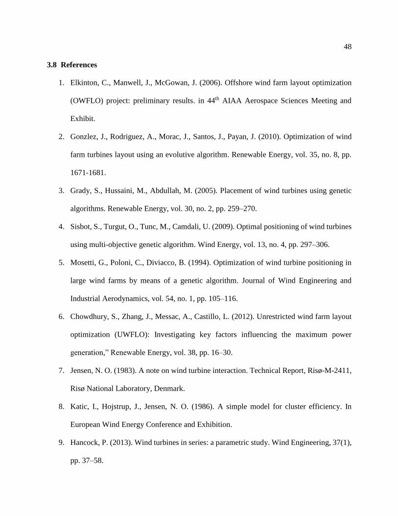
48
3.8 References
1. Elkinton, C., Manwell, J., McGowan, J. (2006). Offshore wind farm layout optimization
(OWFLO) project: preliminary results. in 44th AIAA Aerospace Sciences Meeting and
Exhibit.
2. Gonzlez, J., Rodriguez, A., Morac, J., Santos, J., Payan, J. (2010). Optimization of wind
farm turbines layout using an evolutive algorithm. Renewable Energy, vol. 35, no. 8, pp.
1671-1681.
3. Grady, S., Hussaini, M., Abdullah, M. (2005). Placement of wind turbines using genetic
algorithms. Renewable Energy, vol. 30, no. 2, pp. 259–270.
4. Sisbot, S., Turgut, O., Tunc, M., Camdali, U. (2009). Optimal positioning of wind turbines
using multi-objective genetic algorithm. Wind Energy, vol. 13, no. 4, pp. 297–306.
5. Mosetti, G., Poloni, C., Diviacco, B. (1994). Optimization of wind turbine positioning in
large wind farms by means of a genetic algorithm. Journal of Wind Engineering and
Industrial Aerodynamics, vol. 54, no. 1, pp. 105–116.
6. Chowdhury, S., Zhang, J., Messac, A., Castillo, L. (2012). Unrestricted wind farm layout
optimization (UWFLO): Investigating key factors influencing the maximum power
generation,” Renewable Energy, vol. 38, pp. 16–30.
7. Jensen, N. O. (1983). A note on wind turbine interaction. Technical Report, Risø-M-2411,
Risø National Laboratory, Denmark.
8. Katic, I., Hojstrup, J., Jensen, N. O. (1986). A simple model for cluster efficiency. In
European Wind Energy Conference and Exhibition.
9. Hancock, P. (2013). Wind turbines in series: a parametric study. Wind Engineering, 37(1),
pp. 37–58.

49
10. Okulov, V., van Kuik, G. (2012). The Betz-Joukowsky limit: On the contribution to rotor
aerodynamics by the British, German and Russian scientific schools. Wind Energy, 15(2),
pp. 335–344.
11. Herbert-Accro, J.-F., Franco-Acevedo, J.-R., Valenzuela-Rendon, M., Probst- Oleszewski,
O. (2009). Linear wind farm layout optimization through computational intelligence. In
MICAI 2009, LNAI 5845.
12. Madjidian, D., Rantzer, A. (2011). A stationary turbine interaction model for control of
wind farms. In 18th IFAC World Congress.
13. Marden, J., Ruben, S., Pao, L. (2012). Surveying game theoretic approaches for wind farm
optimization. In Proceedings of the AIAA Aerospace Sciences Meeting.
14. Crasto, G., Castellani, F. (2013). Wakes calculation in an offshore wind farm. Wind
Engineering, 37(3), pp. 269–280.
15. Deb, K. (2001). Multi-objective optimization using evolutionary algorithms. John Wiley
& Sons.
16. Mohamed, M., Wood, D. (2013). Vertical wind speed extrapolation using the k–휀
turbulence model. Wind Engineering, 37(1), pp. 13–36.
17. Rφkenes, K., Krogstad, P. (2009). Wind tunnel simulation of terrain effects on wind farm
siting. Wind Energy, 12(4), pp. 391–410.

50
Chapter 4 : Some Effects of Efficiency on Wind Turbine Interference and Maximum
Power Production
Abstract
The effects of finite efficiency on wake interference and power output are studied for identical
horizontal-axis wind turbines in line with the wind. Interference occurs whenever turbines reduce
the power available to any turbines downwind of them. The analysis uses wake models that are
commonly employed in wind farm layout design. The aerodynamic efficiency is varied from 75%
to 100% for six identical hypothetical turbines in line parallel to the wind direction with spacing
from four to six rotor diameters. Selfish optimization of the power output of individual turbines
and co-operative optimization of the total power are considered. For selfish control, all turbines
operate at the maximum possible local CP, based on the aerodynamic efficiency. For co-operative
optimization, each turbine operates at a CP value between zero and the selfish value, and the total
power is optimized numerically. The results show that at low efficiency, there is little difference
in total power output between the two strategies. As efficiency increases, co-operative
optimization produces increasingly more power. As turbine spacing increases, the difference
between the strategies decreases. There is, however, a realistic range of efficiencies and spacing
over which more power is delivered by co-operative optimization. The simplest form of co-
operative optimization requires reducing the power output of the most upwind turbine to allow
increased performance from those downwind. This should be an easy strategy to implement in
wind farm control.

51
Keywords: Layout optimization, Co-operative optimization, Selfish optimization, Turbines in-
line, Wind farm control.
4.1 Introduction
One of the main challenges in designing a wind farm layout is the minimization of turbine wake
interference. Any upwind turbine necessarily reduces the energy available to any turbine in its
wake, and this interference is obviously maximized when turbines are in line in the direction of
the wind. Hancock [1] formulated the problem of identical ideal turbines in line using two models,
the first from actuator disk theory (ADT) which is the simplest possible, and the second was a
modification that allowed wake recovery. Kiani et al. [2] derived explicit solutions for similar
models and found, for example, that an infinite array of ideal wind turbines can produce only
12.5% more power than a single turbine operating at the Betz-Joukowsky limit. It was also found
that co-operative optimization of all turbines always produced more power than selfish (or
individual) optimization of each turbine. This is, potentially, a valuable result as the current
paradigm in wind farm control is selfish optimization. To justify a move towards co-operative
optimization, it must be demonstrated to be superior for more realistic wake models. Further, it is
necessary to account for the effects of turbine efficiency on the energy remaining in the wind and,
therefore, the performance of the downwind turbines. Efficiency in this context has two
components, the first being the aerodynamic efficiency, 𝜂𝑎, which relates the extracted
(aerodynamic) power coefficient, 𝐶𝑃,𝑎, to that obtained from the ADT analysis at the same 𝐶𝑇. It
is maximized at the Betz-Joukowsky limit and defined as

52
𝜂𝑎 =𝑎𝑒𝑟𝑜𝑑𝑦𝑛𝑎𝑚𝑖𝑐 𝑝𝑜𝑤𝑒𝑟
𝐴𝐷𝑇 𝑝𝑜𝑤𝑒𝑟 = (
𝐶𝑃,𝑎
𝐶𝑃,𝐴𝐷𝑇)
𝐶𝑇
(4.1)
Second, the available power curves of commercial turbines give the electrical output power whose
ratio to the extracted power is the efficiency of power conversion. The conversion efficiency, 𝜂c,
is defined as
𝜂c =𝑐𝑜𝑛𝑣𝑒𝑟𝑡𝑒𝑑 𝑒𝑙𝑒𝑐𝑡𝑟𝑖𝑐𝑎𝑙 𝑝𝑜𝑤𝑒𝑟
𝑎𝑒𝑟𝑜𝑑𝑦𝑛𝑎𝑚𝑖𝑐 𝑝𝑜𝑤𝑒𝑟 = (
𝐶𝑃,𝑐
𝐶𝑃,𝑎)
𝐶𝑇
(4.2)
In this paper the two power coefficients, 𝐶𝑃,𝑎 and 𝐶𝑃,𝑐, and the corresponding thrust
coefficient, 𝐶𝑇, are based on the local wind speed of the turbine. The total power coefficient of the
turbines in line based on the undisturbed wind speed, 𝑈𝑂, is denoted 𝐶𝑃,𝑂.
Only horizontal-axis wind turbines (HAWTs) are considered in this paper. They have complex
wakes whose interaction with downwind turbines is even more complex, e.g. [3]. Many studies of
interfering wind turbines have used sophisticated methods to solve the wake flow, such as large
eddy simulation, which is computationally expensive even on powerful computer clusters, e.g.
[4,5,6,7]. Such models are obviously unsuitable for optimization with present computational
resources. They represent the other extreme from the models used by [1,2]. A satisfactory
compromise that is accurate and useful for control will lie somewhere between these extremes.
This paper attempts to move towards that satisfactory model by using a wake model that is a
common component of current wind farm layout software.
In the next section, the mathematical formulation of the chosen wake model is described. The
determination of the major operational parameters (𝐶𝑃, 𝐶𝑇, and 𝑎) is discussed briefly in section
4.3. Section 4.4 gives the remaining details of the simulations. The results are presented and
discussed in section 4.5, and finally the major conclusions are collected in section 4.6.

53
4.2 Wake Model
Among many wake models that have been developed during the last four decades, Jensen’s is one
of the oldest, simplest, and most accurate, e.g. [8,9]. According to Barthelmie et al. [10], who
evaluated it along with other commonly used wake models: “Overall, it is not possible to establish
any of the models as having individually superior performance with respect to the measurements.”
Further the model “has proven to be reliable for long-term power predictions in small to medium
size wind farms, but tends to underestimate wake losses for large wind farms” [11], especially in
the first few rows, [12]. This model, originally proposed by Jensen [13], was developed further by
Katic et al. [14] and Frandsen [15].
The wake diameter, 𝐷𝑤, and wind speed, 𝑈𝑤, can be estimated at any downstream location, x,
as function of an expansion constant, 𝑘, and the blade local axial induction factor, 𝑎, as:
𝐷𝑤 = 𝐷𝑒𝑥𝑝 + 2𝑘𝑥 (4.3)
𝑈𝑤 = 𝑈 {1 −2𝑎
[1 + 2𝑘. 𝑥/𝐷𝑒𝑥𝑝.]2} (4.4)
𝐷𝑒𝑥𝑝 = 𝐷 [1 − 𝑎
1 − 2𝑎]
1/2
(4.5)
where 𝑎 = 1 −𝑈𝑏
𝑈, 𝐷 is the rotor diameter, 𝐷𝑒𝑥𝑝 is the downstream diameter immediately after
the initial wake expansion [15], 𝑈 is the turbine’s upstream wind speed, and 𝑈𝑏 is the wind speed
at the rotor plane. The value of 𝑘 is taken as 0.075 as recommended by WAsP [16] and WindPro
[17] for onshore wind farms.
Each turbine (except the most upstream) is assumed to be effected by all the upwind ones. The
total velocity deficit of the 𝑖𝑡ℎ turbine is approximated as

54
𝛿𝑈𝑖 = √ ∑ 𝛿𝑈𝑖𝑗 2
𝑗=𝑖−1
𝑗=1
(4.6)
where the contribution of the 𝑗𝑡ℎ turbine (𝑗 < 𝑖) is
𝛿𝑈𝑖𝑗 =2𝑎𝑗
[1 + 2𝑘∆𝑥𝑖𝑗/𝐷𝑒𝑥𝑝,𝑗]2 (4.7)
and ∆𝑥𝑖𝑗 is the distance between the 𝑖𝑡ℎ and 𝑗𝑡ℎ turbines. Thus, the velocity immediately upwind
of turbine i is
𝑈𝑖 = 𝑈0(1 − 𝛿𝑈𝑖) (4.8)
where 𝑈0 is the undisturbed wind speed well upwind of the turbine line.
4.3 Determining the Induction Factor
Wake models normally use the turbine thrust coefficient, 𝐶𝑇, to establish the value of 𝑎. Further,
most optimization studies assumed a fixed value for 𝐶𝑇, typically 0.88, e.g. [18,19,20,21,22],
which is not generally accurate. On the other hand, Acero et al. [23] used the manufacturer’s data
for 𝐶𝑇 for the commercial turbine that they considered. Alternatively, Frandsen [24] proposed a
generic formula for 𝐶𝑇 as function of wind speed:
𝐶𝑇 =3.5(2𝑈 − 3.5)
𝑈2 (4.9)
For an isolated turbine, Figure 4.1 demonstrates that neither 𝐶𝑇 = 0.88 nor Equation (4.9) match
the available manufacturers’ data for commercial turbines, as documented in the Appendix.
The thrust data from Figure 4.1 is re-plotted in Figure 4.2 as a function of 𝐶𝑃 along with the
relation inferred from the basic ADT equations, e.g. [25]:

55
𝐶𝑃 = 4𝑎(1 − 𝑎)2 (4.10)
𝐶𝑇 = 4𝑎(1 − 𝑎) (4.11)
Equation (4.10) was used by [1,2], to determine 𝑎. This over-estimates the power output for a
turbine as well as the available power for the downwind ones. The thrust coefficient for three
turbines (turbines 1-3) was given in terms of 𝐶𝑃,𝑎 while for the other five (turbines 4-8) was based
on 𝐶𝑃,𝑐 .
Figure 4.1: CT vs U for the 8 wind turbines described in the Appendix compared with
Equation (4.9) and CT = 0.88.

56
Figure 4.2: CT vs CP for the 8 wind turbines described in the Appendix compared to that from
Equations (4.10) and (4.11).
4.4 Details of the Simulations
Figure 4.3 shows the two efficiencies for turbines 1-3. Since the wake development depends only
on the aerodynamic efficiency, we decided to simplify the analysis by using only that efficiency.
The wake development and interference were computed for a range of 𝜂𝑎 (0.75 𝜂𝑎 ≤ 1.0) that
exceeds the range shown in Figure 4.3. In other words, 𝑎 was determined from Equation (4.10)
using 𝐶𝑃 = 𝐶𝑃,𝑎/𝜂𝑎, and no use was made of the thrust data for the wake calculations.
It was decided to study six turbines in line as this is typical of wind farm arrangement and large
enough to display the major effects of interference, e.g. [14,26,27]. Calculations were done for
turbine spacings of 4, 5, and 6 rotor diameters on the grounds that interference is greater for smaller
distances and 4 is approximately the minimum used for wind farms.

57
MATLAB scripts were used to obtain the optimum solution for co-operative operation using
the genetic algorithm solver, ga. The decision variable was the local aerodynamic power
coefficient and the objective function for co-operative optimization was the total power. The
population size was 60, and the computations were allowed to evolve for a maximum of 300
generations. The termination criterion in ga, TolFun, defines the tolerance on the converged
solution. It was set at 10-15, which is significantly smaller than the default value of 10-6, in an
attempt to get accurate differences between selfish and co-operative power output when the
difference was very small. Typically, 200 to 250 generations were required for termination. No
optimization algorithm was needed for selfish cases as the local 𝐶𝑃,𝑎 for all turbines were set to
the maximum value of 16 𝜂𝑎 /27.
Figure 4.3: Comparison of the two efficiencies for turbines 1-3. The left Figure shows ηa and
the right ηc.

58
4.5 Results and Discussion
Figure 4.4 and Figure 4.5 present the optimal distribution of 𝐶𝑃,𝑎 and 𝑎, respectively, for all cases.
For the lowest efficiency, 𝜂𝑎 = 0.75, there is very little difference between selfish and co-operative
optimizations. The differences increase with increasing 𝜂𝑎 and are maximized for ideal turbines
with 𝜂𝑎 = 1.0, as studied by [2]. The main difference between the two optimizations occurs for the
first turbine: if it operates co-operatively, then its power output is reduced to increase that of the
downwind machines. As the efficiency increases, the power output of the first turbine rises, but
very slightly. In all cases, the second turbine has the minimum power coefficient, and the last
turbine has the same power coefficient independently of the optimization. As expected, there is an
increase in power output as turbine spacing increases as this increases wake recovery.
Figure 4.4: The local aerodynamic power coefficient for co-operative and selfish cases. From
the top left Figure the values of ηa are 0.75, 0.80, and 0.85. From the bottom left Figure the
values of ηa are 0.90, 0.95, and 1.0.

59
Figure 4.6 shows the contribution of each turbine to the total power output as measured by CP,O,
and Figure 4.7 and Figure 4.8 show the sum of the power coefficients. The difference between the
two optimizations is negligible at the lowest efficiency but becomes significant as efficiency
increases. In all cases of co-operative optimization, the first turbine reduces its output so the
subsequent turbines can produce more. There is almost constant power produced by the second to
sixth turbines, which agree with many experimental and theoretical data, e.g. [26,27]. This leads,
as seen in Figure 4.9, to co-operative optimization generally producing more power than selfish
optimization.
Figure 4.5: The local blade axial induction factor for co-operative and selfish cases. From the
top left Figure the values of ηa are 0.75, 0.80, and 0.85. From the bottom left Figure the values of
ηa are 0.90, 0.95, and 1.0.
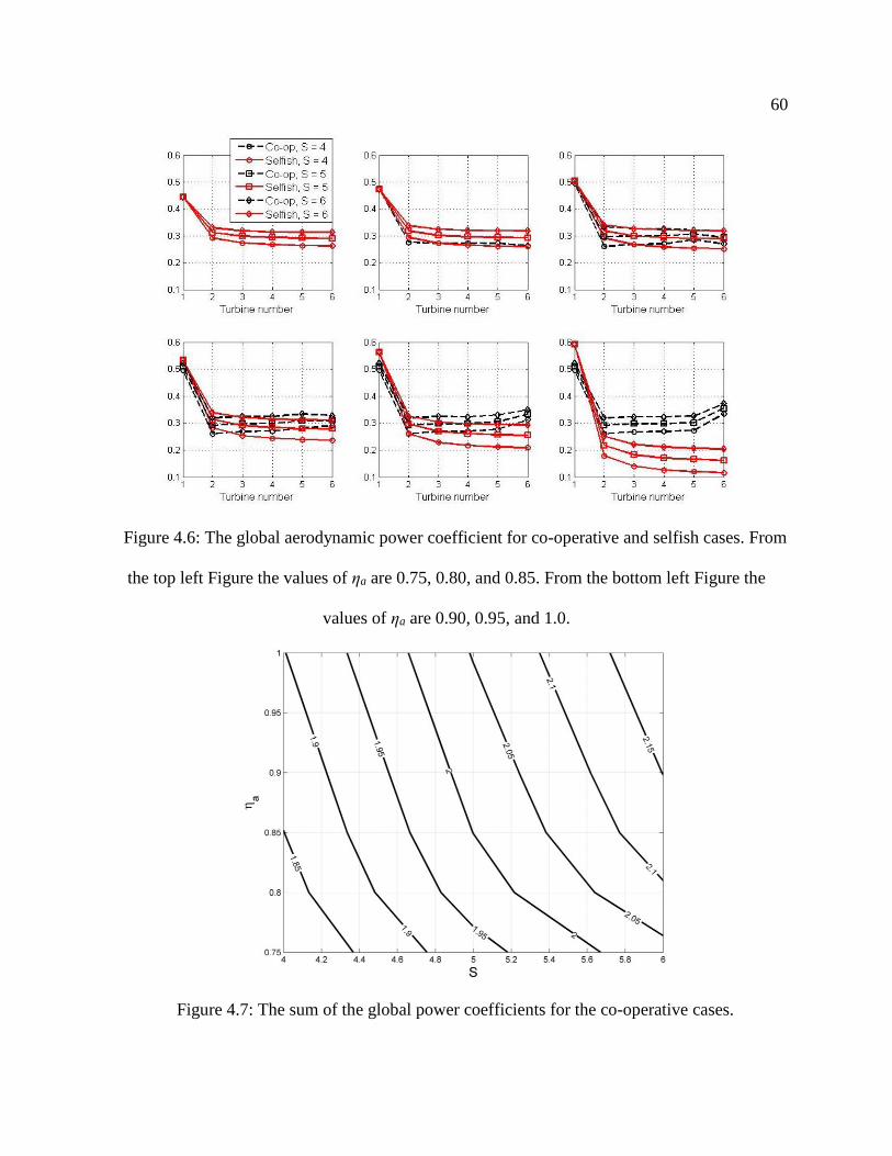
60
Figure 4.6: The global aerodynamic power coefficient for co-operative and selfish cases. From
the top left Figure the values of ηa are 0.75, 0.80, and 0.85. From the bottom left Figure the
values of ηa are 0.90, 0.95, and 1.0.
Figure 4.7: The sum of the global power coefficients for the co-operative cases.

61
Figure 4.8: The sum of the global power coefficients for the selfish cases.
Figure 4.9: The ratio of selfish to co-operative total power.

62
4.6 Conclusions
This paper considers methods to optimize the power output from a straight line of HAWTs parallel
to the wind direction by modelling the significant interference of downwind turbines by upwind
ones. This problem was investigated by [1,2] who assumed ideal turbine behaviour and simple
wake models. They found that co-operative optimization of the total power output always
produced more power than selfish optimization of the individual turbines.
The main aim of this paper was to compare the optimization methods for the more realistic
situation of non-ideal turbines using a wake model that is used in commercial wind farm layout
software. A consideration of the available thrust data for commercial HAWTs showed that it was
preferable to base the wake calculations on the aerodynamic parameters. The aerodynamic
efficiency varied from 0.75 to 1.0, with the upper limit corresponding to an ideal turbine as defined
by standard actuator disk theory.
All calculations were done for six turbines in line at spacing of 4, 5, and 6 rotor diameters on
the grounds that these were representative values. Co-operative optimization can be done
analytically only for simpler wake models than those used here, so we used MATLAB’s genetic
algorithm solver, ga, to perform such. On the other hand, selfish control was computed by adapting
all the N turbines to work at the maximum possible CP,a. The main results were:
1. At low efficiency, there is little difference in total power output between the two
strategies,
2. As efficiency increases, co-operative optimization produces increasingly more power,
3. As turbine spacing increases, the difference between the two strategies decreases, and
4. There is a realistic range of efficiencies and spacing over which more power is delivered
by co-operative optimization.

63
5. Co-operative optimization requires reducing the power output of the most upwind turbine
to allow increased performance from those downwind. This should be an easy strategy to
implement.
Acknowledgments
This research is part of a programme of work on renewable energy funded by the Natural Science
and Engineering Council (NSERC) and the ENMAX Corporation.
64
Appendix to Chapter 4: The technical specifications for the 8 commercial turbines.
S/N Manufacturer Turbine
designation
D
(m)
Rated power
(MW)
Rated speed
(m/s)
1 Sinovel SL1500/89 89.42 1.5 11.5
2 Vestas V90-1.8 90 1.8 13
3 Sinovel SL3000/113-HH90 113.3 3 11
4 Vestas V100-1.8 100 1.815 11.5
5 REpower MM92 92.5 2.050 13
6 Vestas V112-3.0 112 3.075 13
7 REpower 3.2M114 114 3.17 12
8 REpower 3.4M104 104 3.37 14
1- Sinovel (2012). Technical specification SL 1500/89 (CC-60Hz). Sinovel wind group Co.,Ltd.
https://www.edockets.state.mn.us/EFiling/edockets/searchDocuments.do?method=showPoup
&documentId=%7B00FEBE64-5230-48BF-B68F-
96EE5AA5EF09%7D&documentTitle=20124-74025-04 [accessed March 2015].
2- Vestas (2010). General Specification V90–1.8/2.0 MW 50 Hz VCS, Vestas Wind Systems
A/S.
http://ventderaison.eu/gembloux/eie_ABO-
WIND/Annexes/Annexe_N_1_Courbe_acoustique_V90.pdf [accessed March 2015].
3- Sinovel (2011). Specification SL3000 series wind turbine SL3000/113-HH90 (60Hz).
Sinovel wind group Co.,Ltd.
http://www.greenextreme.se/wp-content/uploads/2013/08/Bilagor.pdf [accessed March 2015].

65
4- Vestas (2010). General Specification V100–1.8 MW VCUS, Vestas Wind Systems A/S.
http://www.opsb.ohio.gov/opsb/assets/File/12-0160-12-0160-Vestas%20V100.PDF
[accessed March 2015].
5- Repower (2011). Power Curve & Sound Power Level REpower MM92 [2050 kW], REpower
Systems AG.
http://www.sholland.gov.uk/PublishedRecords/PBC/DC/APP/4/H19-0081-11-H19-0081-
11_V1014400702052013_4DOCS.pdf [accessed March 2015].
6- Vestas (2010). General Specification V112–3.0 MW 50/60 Hz, Vestas Wind Systems A/S.
http://documents.dps.ny.gov/public/Common/ViewDoc.aspx?DocRefId=%7B15E6A798-
4D37-488D-A150-BD6CE70359CE%7D [accessed March 2015].
7- Repower (2011). Power Curve & Sound Power Level REpower 3.2M114[3.2M/114/50Hz],
REpower Systems SE.
http://ventderaison.eu/honnelles/eie_eneco_2013/annexes/annexe_F.pdf [accessed March
2015].
8- Repower (2011). Power Curve & Sound Power Level REpower 3.4M104[3.4M/104/50Hz],
REpower Systems SE.
http://ventderaison.eu/honnelles/eie_eneco_2013/annexes/annexe_F.pdf [accessed March
2015].

66
4.7 References
1. Hancock, P. (2013). Wind turbines in series: A parametric study, Wind Engineering, 37(1),
pp. 37-58.
2. Kiani, A., Abdulrahman, M., Wood, D. (2014). Explicit solutions for simple models of
wind turbine interference. Wind Engineering, 38(2), pp. 167-180.
3. Adaramola, M.S., Krogstad P.-Å. (2011). Experimental investigation of wake effects on
wind turbine performance. Renewable Energy, 36, 2078-2086.
4. Sanderse, B., van der Pijl, S., Koren, B. (2011). Review of computational fluid dynamics
for wind turbine wake aerodynamics. Wind Energy, 14, pp. 799-819.
5. Vogstad, K., Bhutoria, V., Luns, J.A., Ivanell, S., Uzunoglu, B. (2012). Instant wind -
Model reduction for fast CFD computations, Elforsk rapport V-366.
6. Porte-Agel, F., Yu, Y.T., Chen, C-H (2013). A numerical study of the effects of wind
direction on turbine wakes and power losses in a large wind farm. Energies, 6, pp. 5297-
5313.
7. Annoni, J., Seiler, P., Johnson, K., Fleming, P., Gebraad, P. (2014). Evaluating wake
models for wind farm control. American Control Conference, pp. 2517-2523.
8. Sørensen, T., Nielsen, P., Thøgersen, M. L. (2006). Recalibrating wind turbine wake model
parameters – Validating the wake model performance for large offshore wind farms. EMD
International A/S.
9. Sørensen, T., Thøgersen, M. L., Nielsen, P., Jernesvej, N. (2008). Adapting and calibration
of existing wake models to meet the conditions inside offshore wind farms. EMD
International A/S. Aalborg.

67
10. Barthelmie, R.J., Folkerts, L., Larsen, G.C., Rados, K., Pryor, S.C., Frandsen, S.T., Lange,
B., Schepers, G. (2006). Comparison of wake model simulations with offshore wind
turbine wake profiles measured by SODAR. Journal of Atmospheric & Oceanic
Technology, 23(7), pp. 888-901.
11. Schlez, W., Neubert, A. (2009). New developments in large wind farm modelling.
Proceedings of the EWEC, Marseille, France.
12. Beaucage, P., Robinson, N., Brower, M., Alonge, C. (2012). Overview of six commercial
and research wake models for large offshore wind farms. Proceedings of the EWEA
conference, Copenhagen.
13. Jensen, N.O. (1983). A note on wind generator interaction. Risø-M-2411, Risø National
Laboratory.
14. Katic, I., Hojstrup, J., Jensen, N.O. (1986). A simple model for cluster efficiency. In
Proceedings of the European Wind Energy Association Conference and Exhibition, pp.
407–410.
15. Frandsen, S. (1992). On the wind speed reduction in the center of large clusters of wind
turbines. Journal of Wind Engineering and Industrial Aerodynamics, 39, pp. 251-265.
16. Mortensen, N.G., Heathfield, D.N., Myllerup, L., Landberg, L., Rathman, O. (2005). Wind
atlas analysis and application program: WAsP 8 help facility. Risø National Laboratory,
Roskilde, Denmark. ISBN 87-550-3457-8.
17. Nielsen, P. (2006). The WindPRO manual, edition 2.5, EMD International A/S.
18. Mosetti, G., Poloni, C., Diviacco, B. (1994). Optimization of wind turbine positioning in
large windfarms by means of a genetic algorithm. Journal of Wind Engineering and
Industrial Aerodynamics 51(1), pp. 105-116.

68
19. Grady, S.A., Hussaini, M.Y., Abdullah, M.M. (2005). Placement of wind turbines using
genetic algorithms. Renewable Energy 30(2), pp. 259–270.
20. Marmidis, G., Lazarou, S., Pyrgioti, E. (2008). Optimal placement of wind turbines in a
wind park using monte carlo simulation. Renewable Energy, 33, pp. 1455–1460.
21. Emami, A., Noghreh, P. (2010). New approach on optimization in placement of wind
turbines within wind farm by genetic algorithms. Renewable Energy, 35, pp. 1559–1564.
22. Chen, Y., Li, H., Jin, K., Song, Q. (2013). Wind farm layout optimization using genetic
algorithm with different hub height wind turbines. Energy Conversion and Management,
70, pp. 56–65.
23. Acero, J., Acevedo, J., Rendon, M., Oleszewski, O. (2009). Linear wind farm layout
optimization through computational intelligence. Proceedings of 8th Mexican International
Conference on Artificial Intelligence, pp. 692–703.
24. Frandsen, S. (2007). Turbulence and turbulence-generated structural loading in wind
turbine clusters. Risø-R-1188(EN), Risø National Laboratory.
25. Burton, T., Sharpe, D. (2011). Wind energy handbook. John Wiley & Sons Ltd, ISBN 0-
471-48997-2, Chichester, 2nd edition.
26. Crespo, A., Hernandez, J., Frandsen, S. (1999). Survey of modelling methods for wind
turbine wakes and wind farms. Wind Energy, 2, pp. 1–24.
27. Frandsen, S., Barthelmie, R., Pryor, S., Rathmann, O., Larsen, S., Højstrup, J., Thøgersen,
M. (2006). Analytical modelling of wind speed deficit in large offshore wind farms. Wind
Energy, 9, pp. 39–53.

69
Chapter 5 : Investigating the Power-COE Trade-Off for Wind Farm Layout Optimization
Considering Commercial Turbine Selection and Hub Height Variation
Abstract
New aspects were added to the wind farm layout optimization problem by including commercial
turbine selection and a realistic representation for the thrust coefficient. The available
manufacturers’ data were used to develop generic representation for the thrust coefficient, on
which the wake and power calculations mainly depend. A simple field-based cost model was
implemented. The optimization was performed for onshore and offshore conditions using
MATLAB genetic algorithm, ga, solver for two simple test cases. Three objective functions were
considered, individually: (1) the output power, (2) the capacity factor, and (3) the cost per output
power.
The results showed that the flexibility of using different turbines and hub heights can provide a
useful trade-off between power and cost. The trade-off was found to be wider in offshore cases,
which means that the optimization is more useful in such conditions. The optimization for
maximum capacity factor acts as a mid-point between the two design extremes of maximizing
power and minimizing the cost of energy. Almost all turbines were selected at least once in an
optimum layout. However, the priority in selection was for the turbines that have bigger diameter
and/or lower rated speed amongst the other turbines of the same rated power.
Keywords: Wind farm layout optimization, Genetic algorithm, Commercial turbine selection,
Wind turbine thrust, Hub height variation.

70
5.1 Introduction
The expanding wind power market faces several technical and financial challenges related to
output power maximization and cost of energy (COE) minimization. Moreover, many restrictions
have been put on wind farm installations because of environmental impact in the form of noise,
visual effects, and bird and bat interactions. All these factors increase the need for Wind Farm
Layout Optimization (WFLO) which investigates the design of wind farms in order to optimize
the value of one (or more) objective function(s) while satisfying one (or more) constraint(s). The
classical WFLO literature deals mainly with placing identical turbines to maximize energy
production, minimize COE, maximize profit, or a combination of them [1].
Mosetti et al. [2] introduced the WFLO problem. They considered 10×10 square cells of 200
m sides, in which identical 40 m diameter turbines were to be placed. A constant thrust coefficient,
𝐶𝑇 = 0.88, as well as simple cubic power curve were assumed. Jensen’s analytical wake model
[3,4] was used to assess turbine interference and a Genetic Algorithm (GA) was implemented to
maximize a combined objective function including the total power and the inverse of the cost of
energy, using arbitrary weighting factors.
For the following decade, no significant contribution was made to WFLO. New aspects were
then implemented; either to the design variables, constraints, objective functions, and/or to the
optimization methodology. Many researchers have analyzed the problem proposed by Mosetti et
al. in order to obtain better layouts and/or reduce the computational time, either with some
improvements to the GA, e.g. [5,6,7,8] or by implementing other optimization strategies, e.g.
[9,10,11,12,13].
Very few studies have considered non-identical turbines and/or varying hub heights; these will
be reviewed in more detail in the next section. The motivation and the aims of the proposed

71
research are stated at the end of section 5.2. The proposed methodology is explained in detail in
section 5.3. Finally, the primary results for the test cases as well as the major conclusions are the
topics of sections 5.4 and 5.5, respectively.
5.2 Literature Review
Herbert-Acero et al. [14] maximized the power production by a line of turbines in the wind
direction using both Simulated Annealing and a GA implemented in MATLAB. They used the
technical data for the REpower, MD77 turbine with rotor diameter, D = 77 m. Two values of hub
height (H) were used, 50 m and 85 m, to reduce the effect of wake overlap. The design parameters
were the number of turbines, locations, and the individual H, while fixing the line length at 1,550
m (20.13 D). The optimum number of turbines was 6 or 7, which results in average spacing of 4
D and 3.35 D, respectively. The results showed that the placement of wind turbines with different
heights could increase the power generation in a straight line layout for a single wind speed and
two opposite wind directions along the line.
Most actual wind farms employ identical turbines (one model and one H) even if the
installation was done in several stages. It is worth noting, however, that a typical major wind farm
owner owns up to several thousand turbines with a wide range of models and H [15]. For example,
the European fleet maintained directly by EDPR (one of the major owners in Europe) includes 32
turbine models with a wide range of H [16]. In this context, a change from the current situation of
companies owning a large number of farms with identical turbines to varying models and H in
each farm, does not seem like a big change.
Chowdhury et al. [17,18] applied their Unrestricted Wind Farm Layout Optimization
(UWFLO) simultaneously with the appropriate selection of turbines in terms of D (while fixing
72
H), in order to maximize the total power generation. Three different cases were considered: (1)
wind farm with identical turbines, (2) wind farm with differing D, and (3) wind farm with identical
turbines that can adapt to wind conditions (axial induction factor varying on the wind speed) which
can be done for commercial turbines. They found that an optimal combination of wind turbines
with differing rotor diameters can appreciably increase the farm power generation. They
mentioned that a more practical wind farm optimization requires the treatment of rotor diameters
as discrete design variables, as there is only a limited choice of commercial wind turbines.
Chowdhury et al. [19] significantly improved their UWFLO, enabling it to simultaneously
optimize the placement and the selection of turbines for commercial-scale wind farms to minimize
the COE. The number of turbines and the farm size were assumed to be fixed at the values for the
particular wind farm that they studied. They considered the GE 1.5 xle-82.5 as the reference turbine
and normalized the manufacturer’s power curve with respect to the general specifications (rated
power, 𝑃𝑟, cut-in and rated speeds, 𝑈𝑖𝑛 and 𝑈𝑟, respectively). This curve was assumed to be valid
for all commercial turbines and scaled to represent the power curve for any turbine (in the range
0.6 < 𝑃𝑟 < 3.6 MW) as long as the general specifications are defined. The results showed that
simultaneous optimization of the layout and the turbine selection increased the capacity factor by
2% more than that accomplished by layout optimization alone. The optimum layout contained
turbines with 1.8 < 𝑃𝑟 < 3 MW, 90 < D < 110 m, and 80 < H < 120 m.
Chen et al. [20] investigated the use of different H in a small wind farm layout optimization
using GA in MATLAB. They first conducted the layout optimization of a 500 m square wind farm.
Enercon E40m-600kW turbines were used with two values of H (50 and 78 m) and the minimum
turbine proximity of 100 m (2.5 D). Then a larger wind farm (2800 m x 1200 m) with larger wind
turbine (GE 1.62-100) was analyzed to further examine the benefits of using different hub heights

73
(80 and 100 m) in more realistic conditions. The minimum turbine proximity was set as 400 m (4
D). Different cost models were used in the analysis, and results showed that different hub height
wind turbines can increase the power production and/or reduce the COE.
By reviewing the WFLO literature, three deficiencies were identified and led to the research
objectives of the present work:
(5) Selection among the available commercial turbines,
(6) Developing realistic evaluation for commercial turbines’ 𝐶𝑇, and hence the wake
development, and
(7) Investigating the trade-off range between total farm power and COE.
This was done for the basic layout of 6 Turbines In Line (TIL) with the wind as this maximizes
turbine interference, and for a small wind farm (SWF) array consists of 18 turbines. Both typical
onshore and offshore cases were simulated.
5.3 Methodology
In this section, the proposed methodology is presented in detail. In subsection 5.3.1, the wake
model is described first and then the wake interference calculations are formulated. In subsection
5.3.2, the commercial turbines included in the proposed analysis are mentioned and the power
calculations are presented, while subsection 5.3.3 presents the general 𝐶𝑇 representation for
commercial turbines. The investigated range of hub heights is given and justified in subsection
5.3.4, the cost analysis is discussed in subsection 5.3.5, the test cases are described in subsection
5.3.6, and the optimization methodology is illustrated in subsection 5.3.7.

74
5.3.1 Wake model and interference calculations.
Among many wake models that have been developed over the last four decades, Jensen’s analytical
wake model is one of the oldest, simplest, and most accurate in estimating both velocity and power
deficits within wind farms, e.g. [21,22,23,24]. It was also implemented in the majority of WFLO
literature as well as the major WFLO software packages, such as WAsP [25] and WindPro [26].
This model, originally proposed by Jensen [3], was developed by Katic et al. [4] and further by
Frandsen [27]. Referring to Figure 5.1, the wake calculations are as follows:
Figure 5.1: A front view (parallel to wind direction) illustrates the overlap of the upwind turbine
wake (the dashed circle) with the downwind turbine rotor (the solid circle). The Y co-ordinate is
into the page.

75
The wind blows in the positive Y direction, and the turbines were sorted in ascending order
according to their Y coordinates. For example: the most upwind turbine, which has the least Y-
coordinate, was designated 1, while the most downwind one was N (the total number of turbines).
Accordingly, except the most upstream turbine, each turbine i in the farm, 2 < i < N, is potentially
affected by the wake of every upwind turbine j, 1 < j < i-1.
In Figure 5.1, a schematic of the wake interference between upwind and downwind turbines
is given. 𝐻𝑖 and 𝐻𝑗 are the hub heights for the downwind and upwind turbines, respectively, 𝑅𝑖 is
the downwind turbine rotor radius, and 𝑅𝑤,𝑖𝑗 is the radius of the 𝑗𝑡ℎ turbine wake when it reaches
the 𝑖𝑡ℎ turbine [27]
𝑅𝑤,𝑖𝑗 = 𝑅𝑒𝑥𝑝,𝑗 + 𝛼𝑗∆𝑦𝑖𝑗 (5.1)
where
𝑅𝑒𝑥𝑝,𝑗 = 𝑅𝑗√(1 − 𝑎𝑗)/(1 − 2𝑎𝑗) (5.2)
▪ 𝛼𝑗 is the wake expansion coefficient for the 𝑗𝑡ℎ turbine, which is given in terms of the hub
height, 𝐻𝑗, and the site roughness length, 𝑧𝑜, as [27]
𝛼𝑗 = 0.5/𝑙𝑛 (𝐻𝑗
𝑧𝑜) (5.3)
▪ ∆𝑦𝑖𝑗 = 𝑦𝑖 − 𝑦𝑗, is the Y-distance between the two turbines, not shown in Figure 5.1.
▪ The velocity deficit for the 𝑖𝑡ℎ turbine that caused by the wake of the 𝑗𝑡ℎ turbine, 𝛿𝑈𝑖𝑗, is
approximated as
𝛿𝑈𝑖𝑗 = {1 − √1 − 𝐶𝑇,𝑗
[1 + 𝛼𝑗∆𝑦𝑖𝑗/𝑅𝑒𝑥𝑝,𝑗]2} (
𝐴𝑖𝑗
𝐴𝑖) (5.4)
where 𝐴𝑖𝑗 is the overlap of the 𝑗𝑡ℎ turbine wake with the downwind turbine rotor, 𝐴𝑖.

76
▪ The cumulative velocity deficit ahead of the 𝑖𝑡ℎ turbine caused by all upwind turbines is [4]
𝛿𝑈𝑖 = √ ∑ (𝛿𝑈𝑖𝑗)2
𝑗=𝑖−1
𝑗=1
(5.5)
The effective wind speed immediately upwind of the ith turbine is given in terms of the
cumulative velocity deficit and the undisturbed wind speed at Hi, 𝑈𝑜,𝑖 as [3,4]
𝑈𝑖 = 𝑈𝑜,𝑖(1 − 𝛿𝑈𝑖) (5.6)
The following assumptions were made:
(1) The wind has constant speed, direction, and density, 𝜌 = 1.225 𝑘𝑔/𝑚3. Three values were
used (𝑈𝑟𝑒𝑓 = 8, 10, and 12 m/s at 𝐻𝑟𝑒𝑓 = 60 m).
(2) The roughness length, 𝑧𝑂, was taken as 0.3 m for onshore and 0.0002 m for offshore farms.
These values are widely accepted in the WFLO literature.
(3) The log law [28] was used to extrapolate wind speed from the reference height in order to
estimate the undisturbed wind speed at any height, 𝐻𝑚𝑖𝑛 ≤ 𝐻𝑖 ≤ 𝐻𝑚𝑎𝑥
𝑈𝑜,𝑖 = 𝑈𝑟𝑒𝑓 [𝑙𝑛(𝐻𝑖 𝑧𝑜⁄ )
𝑙𝑛(𝐻𝑟𝑒𝑓 𝑧𝑜⁄ )] (5.7)
For each 𝑈𝑟𝑒𝑓 the electrical power output of any turbine depends on its location relative to all
its upwind turbines, the type, H, and 𝐶𝑇 for all upwind turbines, and its type (in terms of its power
curve) and H.
The wake model was validated against the energy production data for Horns Rev 1 offshore
wind farm (as one of the most famous large wind farms worldwide). The farm layout and turbines’
power curve are available in [29], wind resource assessment over three years for the farm site
(before installation) is available in [30], while the details of farm energy production are found in
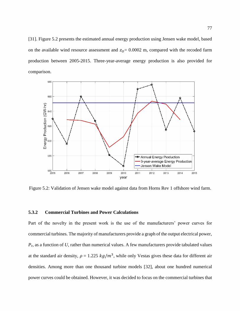
77
[31]. Figure 5.2 presents the estimated annual energy production using Jensen wake model, based
on the available wind resource assessment and 𝑧𝑂= 0.0002 m, compared with the recoded farm
production between 2005-2015. Three-year-average energy production is also provided for
comparison.
Figure 5.2: Validation of Jensen wake model against data from Horns Rev 1 offshore wind farm.
5.3.2 Commercial Turbines and Power Calculations
Part of the novelty in the present work is the use of the manufacturers’ power curves for
commercial turbines. The majority of manufacturers provide a graph of the output electrical power,
Pe, as a function of U, rather than numerical values. A few manufacturers provide tabulated values
at the standard air density, 𝜌 = 1.225 𝑘𝑔/𝑚3, while only Vestas gives these data for different air
densities. Among more than one thousand turbine models [32], about one hundred numerical
power curves could be obtained. However, it was decided to focus on the commercial turbines that

78
fall in the most popular range of rated power (1.5 < 𝑃𝑟 < 3.0 MW). To this end, 61 commercial
turbines from 15 manufacturers in 8 countries were included in the analysis. The selected turbines
cover a wide range of rotor diameter (66 𝑚 ≤ 𝐷 ≤ 115 𝑚) and rated speed (11 𝑚/𝑠 ≤ 𝑈𝑟 ≤
17 𝑚/𝑠). The 61 curves were fitted by a 5th degree polynomial, and the coefficients were used to
estimate the power developed by each turbine at any wind speed between 𝑈𝑖𝑛 and 𝑈𝑟. For wind
speeds above rated speed, the power output was taken as the rated value. Note that no simulations
were done for wind speeds greater than the cut-out speed. Accordingly, the power developed by
the 𝑖𝑡ℎ turbine based on its type and the effective wind speed, 𝑈𝑖 determined as per the previous
section, is estimated as
𝑃𝑖 = 𝑐𝑖0 + 𝑐𝑖1𝑈𝑖 + 𝑐𝑖2𝑈𝑖2+ 𝑐𝑖3𝑈𝑖
3 + 𝑐𝑖4𝑈𝑖4
+ 𝑐𝑖5𝑈𝑖
5= ∑ 𝑐𝑖𝑘𝑈𝑖
𝑘
𝑘=5
𝑘=0
(5.8)
The total farm output power is simply the sum of the individual powers from the N turbines
𝑃 = ∑ 𝑃𝑖
𝑁
𝑖=1
= ∑ ∑ 𝑐𝑖𝑘𝑈𝑖𝑘
𝑘=5
𝑘=0
𝑁
𝑖=1
(5.9)
and the farm capacity factor (CF) is defined as
𝐶𝐹 =𝑂𝑢𝑡𝑝𝑢𝑡 𝑃𝑜𝑤𝑒𝑟
𝑅𝑎𝑡𝑒𝑑 𝑃𝑜𝑤𝑒𝑟=
∑ ∑ 𝑐𝑖𝑘𝑈𝑖𝑘𝑘=5
𝑘=0𝑁𝑖=1
∑ 𝑃𝑟,𝑖𝑁𝑖=1
(5.10)
5.3.3 Commercial Turbine Coefficients
The major wind turbine operational parameters are the power and thrust coefficients. As shown by
Equation (5.4), 𝐶𝑇 is required for wake analysis, however, thrust data is rarely available and one
of the greatest challenges in WFLO is the lack of accurate 𝐶𝑇, e.g. [19]. For this reason, many
WFLO analyses assumed a fixed value for 𝐶𝑇, usually 0.88, e.g. [2,5,9,7,20]. However, it is not

79
accurate in comparison with the available 𝐶𝑇 curves for commercial turbines, [33]. It was found
by simple calculations that an underestimation of 𝐶𝑇 by 0.1 typically results in a significant
underestimation in 𝛿𝑈𝑖𝑗 by about 2-3 %, which overestimates the power output of a downstream
turbine by 6-10 %. In order to obtain a general and practical representation for the thrust
coefficient, the available 𝐶𝑇 data for thirteen commercial turbines (eight from Vestas, three from
REpower, and two from Sinovel) were used to develop two general representations for 𝐶𝑇 in terms
of the aerodynamic and the electric power coefficients, 𝐶𝑃,𝑎 and 𝐶𝑃,𝑒, respectively. The electric
power is simply the turbine output power given by the manufacturer as function of the approaching
wind speed, while the aerodynamic power is defined as the turbine output power if the mechanical
and conversion losses are neglected. These two generic curves are given in Figure 5.3 along with
the results obtained by WT_Perf BEM theory code for NREL 5 MW reference turbine for different
values of pitch angle, 𝛽 [34]. It is clear that the 𝐶𝑇-𝐶𝑃,𝑎 curve matches well with that for NREL
turbine at different pitch angles, which give confidence to the proposed generalization. Finally, the
𝐶𝑇-𝐶𝑃,𝑒 (the dashed line in Figure 5.3) was fitted by a 5th degree polynomial and used to estimate
the thrust coefficient for any turbine once the electric power coefficient is evaluated.

80
Figure 5.3: General representation for the thrust coefficient, CT, vs the aerodynamic and the
electric power coefficients, CP,a and CP,e, respectively, compared with CT - CP,a curves obtained
for NREL 5 MW reference turbine at different values of pitch angle, β.
5.3.4 Hub Height Variation
It is essential to specify the minimum and maximum H (𝐻𝑚𝑖𝑛 and 𝐻𝑚𝑎𝑥) to be investigated. For
𝐻𝑚𝑖𝑛, the “minimum ground clearance” recommendations were taken into account, while 𝐻𝑚𝑎𝑥
should be set by the technology available to install and operate turbines on tall towers. The ground
clearance of a commercial turbine is the height of the blade tip at its lowest position (when the
blade is vertically down). The minimum practical value was taken as 75 ft. (22.86 m), e.g. [35].
Accordingly, 𝐻𝑚𝑖𝑛 for the largest rotor diameter included in the current study (Dmax=115 m) is
𝐻𝑚𝑖𝑛= (115/2) + 22.86 = 80.36 m.

81
On the other hand, taller towers are usually employed to avoid the large wind shear and high
turbulence level at relatively low heights caused partly by the topography, [36]. Engström et al.
[36] described welded steel shell towers for large turbines and concluded that the available
technology can provide towers up to 150 m for 3 MW turbines. Moreover, many operating turbines
were installed with H > 140 𝑚, e.g. [37]. To this end, the lower and upper limits for H in the
analysis were taken as 80 m and 140 m, respectively.
5.3.5 Simple Cost Model
Since the pioneering work by Mosetti et al., many cost models have been developed in order to
implement the COE as an objective function in WFLO [38,1]. The majority of these models were
based on assumptions, local experience, and/or limited available data. The cost of wind farm
installation as well as COE varies significantly over time and location, e.g. [39]. The number of
turbines, the distance from the manufacturer, the cost of land and infrastructure, material and labor
costs, etc. significantly affect the total farm cost as well as the COE. Accordingly, it was decided
to simplify the cost analysis by parameterization in terms of the main design variables (𝑃𝑟 and H)
as far as possible. The major wind power cost reports were reviewed and the following conclusions
were drawn:
i. The Capital Cost (CC) is the major component of the Total Cost (TC) of a wind power
project. Its fractional contribution ranges from 0.70 - 0.83 of the Levelized Cost of
Electricity (LCOE) in the major European countries to 0.89 in USA [40].
ii. The operations and maintenance (O&M) costs of wind power can be represented in $/kW,
$/kW-yr, $/MW-h, or as a percentage of the LCOE, e.g. [40,41,42].
82
iii. The average cost/kW for offshore wind farms is almost double that for onshore ones, also
the O&M cost share (𝐶𝑂&𝑀) is larger in offshore projects, e.g. [40,41].
iv. The turbine capital cost represents about 0.68 of the CC for onshore and about 0.32 for
offshore projects. The tower cost share (𝐶𝑡𝑜𝑤𝑒𝑟) represents approximately 0.12 and 0.0565
of the CC for onshore and offshore projects, respectively [43].
In order to develop a simple and general cost model, the following assumptions were made:
a. Turbine cost was assumed to be determined by the rated power and hub height only. Also
the turbines were assumed equally available everywhere, accordingly the factor of
proximity from the manufacturers was disregarded.
b. The CC was represented in terms of the turbines’ rated power and hub height, while the
O&M costs were determined as a fraction of the TC over the entire lifespan, and
independent of layout.
c. It was decided to set 𝐶𝑂&𝑀 as 0.15 and 0.25 of the TC over the entire lifespan for onshore
and offshore farms, respectively.
d. The minimum H (𝐻𝑚𝑖𝑛 = 80 m) was assumed to be the reference tower height, which also
matches with the common practice for multi-MW turbine towers.
e. The CC of 1.0 MW at 𝐻𝑚𝑖𝑛 was taken as the unit cost and was denoted by Capital Cost
Index (CCI).
f. The increase in H was assumed to be added linearly to the CCI, i.e. each increase of 1.0 m
above 𝐻𝑚𝑖𝑛 adds 1/80 of the contribution of the tower cost to the CC.
Accordingly, the Total Cost Index (TCI) was calculated using the general formula

83
𝑇𝐶𝐼 =𝐶𝐶𝐼
1 − 𝐶𝑂&𝑀= (
1
1 − 𝐶𝑂&𝑀) ∑ 𝑃𝑟,𝑖 [1 +
𝐶𝑡𝑜𝑤𝑒𝑟
𝐻𝑚𝑖𝑛
(𝐻𝑖 − 𝐻𝑚𝑖𝑛)]
𝑁
𝑖=1
(5.11)
where 𝑃𝑟,𝑖 is the rated power of the 𝑖𝑡ℎ turbine (in MW).
It is worth noting here that “total” in TCI is strictly not correct, as the financial and balance of
system costs are not included in Equation (5.11). However, the effect on the calculation is
negligible because these costs depend mainly on the turbines citing which was assumed fixed in
the SWF cases and slightly changes along a specified line length in the TIL ones.
Finally, the Total Cost Index per Output Power (TCIOP) as the TCI divided by the output
power (similar to the COE) is the third objective function.
5.3.6 Test cases
Before applying the proposed optimization methodology to real wind farms, it was decided to
consider simpler test cases in order to examine the effect of the investigated parameters on the
different optimum designs. Two arrangements were analyzed (1) turbines in line with the wind
direction, and (2) a small wind farm. For all cases, the wind direction was in the direction of the
turbines in Figure 5.4a. This Figure shows the simplest wind farm layout, the turbine in line, and
the extreme case of wake interference [44,33]. This simple arrangement is suitable for examining
the effect of turbine selection and hub height variation on the different optimum layouts. N = 6 is
typical of wind farm rows and large enough to display the major effects of interference, e.g.
[4,45,46,44,1]. The total length of the line, LY, was specified based on N, an arbitrary spacing
multiplier, S, and nominal diameter, 𝐷𝑛𝑜𝑚𝑖𝑛𝑎𝑙. The nominal diameter was taken as the diameter of
the largest rated power turbine in the dataset used in this work, which has a rated power of 3.075
MW and 112 m rotor diameter.

84
𝐿𝑌 = (𝑁 − 1) 𝑆𝐷𝑛𝑜𝑚𝑖𝑛𝑎𝑙 (5.12)
Three values of S were investigated (4, 5, and 6), giving three values for LY: 2.24, 2.80, and
3.36 km, respectively. The reason for using fixed N and LY was to allow later comparison among
the different optimum layouts and a reference (un-optimized) design. The reference design was
simply N equally spaced turbines of largest rated power installed at maximum investigated height
(H = 140 m). It is important to emphasize here that S was used initially to specify the line length.
Except of the reference design, the turbines can be located anywhere along the line during the
optimization as long as the minimum turbine proximity constraint is satisfied.
The second test case was for small wind farm array of m columns parallel to the wind and n
rows normal to the wind direction, where m = 3 and n = 6 (so N = 18). The same values for S, LY,
and Uref (as given in TIL test case) were investigated. The spacing multiplier in the crosswind
direction was 3, fixed in all optimizations, so the farm crosswind length was fixed (LX = 672 m).
It was decided to fix the turbine locations during the optimizations in order to direct the
optimization towards the turbine selection (which is the main aspect) as well as H variation.
However, two common configurations were used (array and staggered) as shown in Figure 5.4b
and Figure 5.4c, respectively. Again, the reference design for each configuration contains 18
largest turbines at H = 140 m.

85
Figure 5.4: Reference TIL, array, and staggered SWF layouts.
5.3.7 Optimization
Any optimization problem, including the WFLO, consists of four fields: the design variable(s), the
constraint(s), the optimization objective(s), and the optimization technique, e.g. [38,1]. In this
subsection, the treatment of these four parts in the proposed methodology is explained.
5.3.7.1 Design Variables.
The design (or decision) variable is a parameter that needs to be determined (adjusted) in order to
achieve the optimum solution. The design variables must have upper and lower limits within which
the feasible solutions could be obtained. For the first test case, three variables are to be evaluated
for each turbine: location Y, type, and H, while the turbine locations for the second test case are
fixed. Accordingly, the number of design variables are 18 and 36 for TIL and SWF, respectively.

86
5.3.7.2 Constraints
Optimization problems are usually subjected to restrictions (constraints), and hence not all
solutions are feasible. The upper and lower limits for the design variables are the simplest form of
constraints, and the integer constraint is another example, in which one (or more) of the variables
is (are) necessarily integer. The following constraints were involved in the proposed problem:
▪ The location of any turbine, 𝑖, (1 ≤ 𝑖 ≤ 𝑁) in the TIL case was bounded by the line length (linear
constraint)
0 ≤ 𝑦𝑖 ≤ 𝐿𝑌 (5.13)
▪ The hub height for any turbine was bounded by the minimum and maximum investigated value
of H (linear integer constraint)
𝐻𝑚𝑖𝑛 ≤ 𝐻𝑖 ≤ 𝐻𝑚𝑎𝑥 (5.14)
▪ The selection among the commercial turbines is a linear integer constraint. The 61 turbines were
sorted based on the rated power in an ascending order. The turbines then coded and any turbine
in the farm was allowed to take any integer value from 1 to 61.
1 ≤ 𝑐𝑜𝑑𝑒𝑖 ≤ 61 (5.15)
▪ The minimum turbine proximity was used for TIL optimizations, in which the minimum distance
between any two turbines was set as 3𝐷𝑛𝑜𝑚𝑖𝑛𝑎𝑙. Accordingly, the following condition was
applied
∆𝑦𝑖𝑗 = 𝑦𝑖 − 𝑦𝑗 ≥ 3𝐷𝑛𝑜𝑚𝑖𝑛𝑎𝑙 (5.16)
where, 1 ≤ 𝑖, 𝑗 ≤ 𝑁 and 𝑖 ≠ 𝑗; which results in ∑ 𝑘𝑁𝑘=2 = 20 linear constraint equations.

87
5.3.7.3 Optimization objectives
The objective (fitness) function is simply the variable to be optimized (maximized or minimized).
As mentioned before, three objective functions were considered, individually, in this work: total
power, Equation (5.9), farm capacity factor, Equation (5.10), and total cost index per output power,
determined from Equation (5.11) divided by Equation (5.9).
5.3.7.4 Optimization technique
The best optimization technique depends mainly on the nature of the problem as well as the
constraints. The present optimization problem is discrete, non-linear, non-convex (as it has many
local minima), of very high dimension (each turbine has 61 probabilities in both turbine selection
and H), and mixed integer. GAs have been proven a powerful tool for such complex problems, e.g.
[47]. For this reason, a GA was implemented in the majority of the WFLO literature, although it
is slow compared with the other optimization methods [38,1]. GAs are computer programs that
mimic the processes of biological evolution in order to solve problems and to model evolutionary
systems [48]. The solution is obtained by moving from one population of chromosomes (feasible
solutions) to a new population by using a kind of natural selection (random search) together with
the genetics-inspired operators of crossover, mutation, inversion, etc. Each chromosome consists
of a number of genes that are the possible values of the design variables. The selection operator
chooses those chromosomes in the population that will be allowed to reproduce, and on average
the fitter chromosomes produce more offspring than the less fit ones [48].
The MATLAB ga solver was used to obtain the optimum layouts. The population size (number
of feasible solutions) was set as large as possible to widen the random search in order to increase
the probability of finding the global optimum solution instead of local optima. The chromosomes

88
were allowed to evolve up to 3,000 generations unless the algorithm stops because the average
relative change in the best fitness function value is less than or equal to an arbitrary value called
TolFun. This value was set as low as 10-15 compared with the default value, 10-6, in order to ensure
that the solution is optimal. The stopping criterion was satisfied (and hence the algorithm was
terminated and the optimum solution was obtained) after 1,500 to 2,500 generations in the majority
of the test cases presented in this paper. A flowchart is given in Figure 5.5 for the GA procedure.
Figure 5.5: Flowchart for Genetic Algorithm.
5.4 Results, and Discussion
In this section the results are presented and analyzed and the major findings are discussed. The
power output and the total cost index of the un-optimized design will be referred as “reference

89
power” and “reference cost”, respectively. The optimization for minimum TCIOP will be referred
as “min TC” for brevity.
Figure 5.6a, b, and c present the results for the onshore TIL optimizations for Uref = 8, 10, and
12 m/s, respectively, while Figure 5.7a, b, and c are for the offshore ones. The total power, P, and
the total cost index, TCI, are normalized with respect to that for the corresponding reference layout
in order to get clear comparisons. The main results are summarized as:
1. The reference cost was always the maximum cost, as it contains the largest turbines and max H.
However, the reference power was not the maximum, except for the onshore conditions at high
wind speed at which P from all optimizations, except min TC, collapse to the reference power.
2. As expected; the optimization for max P and min TC are two design extremes. The optimization
of max CF gives results between these extremes, except for high wind speed conditions when
it tends to collapse to the max P optimization.
3. Between the two design extremes there is a relatively wide band of both P and TCI which is, in
all cases, shifted up for normalized P compared with that for normalized TCI. These two
observations are very important and beneficial. The existence of the two bands gives many
feasible designs for the P-TCI trade-off. Moreover, the upward shift of normalized P implies
that lower cost well-designed layouts can develop equal to (or even higher than) power that
can be developed by higher cost improperly designed ones.
4. For the same Uref, N, and farm area the onshore cases developed power up to double that of the
offshore ones (especially at low Uref), however, the latter gave higher normalized power as
well as wider trade-off range. These two observations have the same origin which can be
explained as follows: the onshore roughness length, z0, is much larger, which cause more wind
shear. As the reference wind speed was given at a particular height, the wind speed was higher

90
for the larger z0 at higher H. Moreover, the larger the z0 the higher the entrainment and the
wake velocity through the wake, according to Equations (5.3) and (5.4), respectively. All these
reasons make the onshore cases develop much more power and, in the same time, make the
optimization more effective in the offshore cases (especially at lower Uref and/or S).
(5.6a) Uref. = 8 m/s.
(5.6b) Uref. = 10 m/s.

91
(5.6c) Uref. = 12 m/s.
Figure 5.6: Normalized P and TCI to the reference layout for onshore TIL as a function of S.
(5.7a) Uref. = 8 m/s.

92
(5.7b) Uref. = 10 m/s.
(5.7c) Uref. = 12 m/s.
Figure 5.7: Normalized P and TCI to the reference layout for offshore TIL as a function of S.
Figure 5.8a, b, and c present the onshore SWF optimizations for Uref = 8, 10, and 12 m/s,
respectively, while Figure 5.9a, b, and c are for the offshore condition. As mentioned earlier, the

93
turbine locations were fixed as one of the two configurations in Figure 5.4 (b and c). Moreover, it
was decided to exclude the max CF optimization results in order to keep the Figures clear and
understandable. Layouts with fixed turbine type with variable H are also provided for both array
and staggered configurations in order to present the effect of H variation. Again, P and TCI for
array and staggered configurations are normalized relative to that for the un-optimized array
layout.
The general trends for SWF results are quite similar (qualitatively) to those for the TIL ones,
the other findings are summarized below:
1. As expected, the staggered configuration was superior; it can develop power up to 1.15 and
1.4 times the array one for onshore and offshore conditions, respectively.
2. The staggered SWF has the widest P-TCI trade-off band, especially for the offshore conditions,
the TIL comes second, while the array SWF offers a relatively narrow band.
3. The hub height variation was very efficient in optimization, especially for staggered offshore
conditions with low Uref and/or S, with the maximum normalized power of 1.82, at S = 4, with
almost the same reference cost, as seen in Figure 5.9a.

94
(5.8a) Uref. = 8 m/s.
(5.8b) Uref. = 10 m/s.

95
(5.8c) Uref. = 12 m/s.
Figure 5.8: Normalized P and TCI to the reference layout for onshore SWF as a function of S.
(5.9a) Uref. = 8 m/s.

96
(5.9b) Uref. = 10 m/s.
(5.9c) Uref. = 12 m/s.
Figure 5.9: Normalized P and TCI to the reference layout for offshore SWF as a function of S.

97
For the sake of brevity and as the P-COE trade-off is the main aspect, it was decided not to
present the resulted optimum layouts for the test cases in detail. However, the frequency of turbine
and H selection for TIL optimizations are given in Figure 5.10, the technical data for the six most
selected turbines is provided in Table 5.1. Finally, general remarks about turbine selection for all
cases are given below
Figure 5.10: Frequency of turbine and H selection for TIL cases.

98
Turbine code Rated power
(MW)
Diameter
(m)
Rated speed
(m/s)
61 3.075 112 13
56 3.0 112 12
19 1.8 100 12
45 2.5 115 12
1 1.5 77 13
6 1.5 82 12
Table 5.1: Technical data for the six most selected turbines in decreasing order.
1. Almost all the investigated turbines were selected at least once in an optimum design (only two
turbines were never selected). This confirms that any commercial turbine could be used
somewhere in the farm at certain conditions to obtain an optimum farm design based on the
desired objective(s).
2. The superior turbines (those selected most often) have lower Ur and larger D amongst the
turbines of the same rated power. These turbines develop higher power at any wind speed so
the selection for max P optimizations was entirely among them. The second group of turbines
selected in many layouts were those with large D but higher Ur. The turbines that have lower
Ur and smaller D came third, while those of higher Ur combined with smaller D were rarely
selected.
3. At low wind speeds, the CF optimizations tend to mix medium and large size turbines providing
that the CF is kept high but the total power falls between P and TC optimizations. As the wind

99
speed increases, the medium turbines are replaced by larger ones as they can operate at high
CF, this results in increasing the power output to approach the max P optimizations at higher
wind speeds.
4. The max P optimizations generate feasible layouts by using larger turbines as well as elevated
heights in order to increase the power output. At some locations (especially at lower Uref and/or
S) the higher heights cause accumulation of wake deficits so one turbine should have a lower
H in order to allow the wakes to recover for the rest of the downwind turbines.
5. The min TC optimizations have the opposite trend, with smaller to medium size turbines with
low H being in the majority. At some locations some turbines should escape from the wake
accumulation by having higher H in order to increase the power to reduce the overall TCI. The
chosen turbines, usually of low to medium size also reduce the tower cost, as it depends on the
turbine size.
6. At higher wind speeds and/or S, larger turbines can be used in many places for max CF and
even for min TC optimizations as long as CF kept high and TC kept low, respectively.
5.5 Conclusions
Based on the proposed approach for optimizing the layout of wind farms, and by analyzing the
results for the test cases; we conclude:
1. The analysis provides strong reasons to suggest that wind farm design with identical
turbines should be abandoned in favour of using a range of commercial turbines and hub
heights.

100
2. The optimization for maximum power and minimum cost of energy are the extreme designs
bounding a wide band of optimum designs. Maximizing the capacity factor is one example
between the extremes.
3. Taller towers are needed, not only to reach higher wind speeds, but also to reduce wake
effects, especially in compact wind farm layouts, by exploiting hub height variation.
4. The optimization is more effective in offshore wind farms because of the low entrainment
which delays the wake recovery.
5. The diversity of the 61 commercial turbines used in his study is found to be beneficial in
optimizing the wind farm design, as each turbine could be the optimum selection
somewhere inside the farm at a particular hub height.
6. The priority in selection among commercial turbines having the same rated power (and the
same cost as well) is the larger diameter combined with lower rated speed, followed in
order by larger diameter with higher rated speed, the smaller diameter with lower rated
speed, and finally the smaller diameter combined with higher rated speed.
ACKNOWEDGEMENTS
This research is part of a program of work on renewable energy funded by the Natural Science and
Engineering Council (NSERC) and the ENMAX Corporation. The first author also acknowledges
the Egyptian Government and Prof. El-Adl El-Kady for sharing the fund and supervision during
the early (and the important) part of this work.

101
5.6 References
1. Tesauro, A., Réthoré, P-E, Larsen, G.C. (2012). State of the art of wind farm optimization.
Proceedings of European Wind Energy Conference & Exhibition, European Wind Energy
Association (EWEA 2012), Copenhagen, Denmark.
2. Mosetti, G., Poloni, C., Diviacco, B. (1994). Optimization of wind turbine positioning in
large wind farms by means of a genetic algorithm. Journal of Wind Engineering and
Industrial Aerodynamics, 51, pp. 105-116.
3. Jensen, N.O. (1983). A note on wind generator interaction. Risø-M-2411, Risø National
Laboratory.
4. Katic, I., Hojstrup, J., Jensen, N.O. (1986). A simple model for cluster efficiency. In
Proceedings of the European Wind Energy Association Conference and Exhibition, pp.
407–410.
5. Grady, S.A., Hussaini, M.Y., Abdullah, M.M. (2005). Placement of wind turbines using
genetic algorithms. Renewable Energy, 30(2), pp. 259-270.
6. Hou-Sheng, H. (2007). Distributed genetic algorithm for optimization of wind farm annual
profits. International Conference on Intelligent Systems Applications to Power Systems,
ISAP 2007, Kaohsiung, Taiwan.
7. Emami, A., Noghreh, P. (2010). New approach on optimization in placement of wind
turbines within wind farm by genetic algorithms. Renewable Energy, 35, pp. 1559–1564.
8. Chen, L., MacDonald, E. (2012). Considering landowner participation in wind farm layout
optimization. Journal of Mechanical Design, 134, 084506-1:6.
9. Marmidis, G., Lazarou, S., Pyrgioti, E. (2008). Optimal placement of wind turbines in a
wind park using monte carlo simulation. Renewable Energy, 33, pp. 1455–1460.

102
10. González, J.S., Gonzalez Rodriguez, A.G., Mora, J.C., Santos, J.R., Payan, M.B. (2010).
Optimization of wind farm turbines layout using an evolutive algorithm. Renewable
Energy, 35(8), pp. 1671-1681.
11. Ituarte-Villarreal, C.M., Espiritu, J.F. (2011). Wind turbine placement in a wind farm using
a viral based optimization algorithm. Procedia Computer Science, 6, pp. 469–474.
12. Turner, S.D.O., Romero, D.A., Zhang, P.Y., Amon, C.H., Chan, T.C.Y. (2014). A new
mathematical programming approach to optimize wind farm layouts. Renewable Energy
63(c), pp. 674–680.
13. Zhang, P.Y., Romero, D.A., Beck, J.C., Amon, C.H. (2014). Solving wind farm layout
optimization with mixed integer programming and constraint programming. EURO Journal
on Computational Optimization, 2(3), pp. 195-219.
14. Herbert-Acero, J-F., Franco-Acevedo, J-R., Valenzuela-Rendon, M., Probst-Oleszewski,
O. (2009). Linear wind farm layout optimization through computational intelligence.
Proceedings of 8th Mexican International Conference on Artificial Intelligence, pp. 692–
703.
15. http://www.thewindpower.net/owners_en.php [last access: August 2016].
16. Sierra, A. H., Pérez, E. G. (2013). Wind farm owner’s view on rotor blades – from O&M
to design requirements IQPC - Advances in Rotor Blades for Wind Turbines, Bremen,
Germany.
17. Chowdhury, S., Messac, A., Zhang, J., Castillo, L., Lebron, J. (2010). Optimizing the
unrestricted placement of turbines of differing rotor diameters in a wind farm for maximum
power generation. ASME 2010 International Design Engineering Technical Conferences

103
and Computers and Information in Engineering Conference, Paper No. DETC2010-29129,
pp. 775-790.
18. Chowdhury, S., Zhang, J., Messac, A., Castillo, L. (2012). Unrestricted wind farm layout
optimization (UWFLO): Investigating key factors influencing the maximum power
generation. Renewable Energy, 38(1), pp. 16–30.
19. Chowdhury, S., Zhang, J., Messac, A., Castillo, L. (2013). Optimizing the arrangement and
the selection of turbines for wind farms subject to varying wind conditions. Renewable
Energy, 52, pp. 273-282.
20. Chen, Y., Li, H., Jin, K., Song, Q. (2013). Wind farm layout optimization using genetic
algorithm with different hub height wind turbines. Energy Conversion and Management,
70, pp. 56–65.
21. Sørensen, T., Nielsen, P., Thøgersen, M.L. (2006). Recalibrating wind turbine wake model
parameters – Validating the wake model performance for large offshore wind farms. EMD
International A/S.
22. Sørensen, T., Thøgersen, M.L., Nielsen, P., Jernesvej, N. (2008). adapting and calibration
of existing wake models to meet the conditions inside offshore wind farms. EMD
International A/S.
23. Barthelmie, R.J., Folkerts, L., Larsen, G.C., Rados, K., Pryor, S.C., Frandsen, S.T., Lange,
B., Schepers, G. (2006). Comparison of wake model simulations with offshore wind
turbine wake profiles measured by SODAR. Journal of Atmospheric & Oceanic
Technology, 23(7), pp. 888-901.

104
24. Beaucage, P., Robinson, N., Brower, M., Alonge, C. (2012). Overview of six commercial
and research wake models for large offshore wind farms. Proceedings of the EWEA
conference, Copenhagen.
25. Mortensen, N.G., Heathfield, D.N., Myllerup, L., Landberg, L., Rathman, O. (2005). Wind
atlas analysis and application program: WAsP 8 help facility. Risø National Laboratory,
Roskilde, Denmark.
26. Nielsen, P. (2006). The WindPRO Manual Edition 2.5, EMD International A/S.
27. Frandsen, S. (1992). On the wind speed reduction in the center of large clusters of wind
turbines. Journal of Wind Engineering and Industrial Aerodynamics, 39, pp. 251-265.
28. Oke, T.R. (1987). Boundary layer climates. 2nd Edition, Methuen, London.
29. Jensen, L., Mørch, C., Sørensen, P., Svendsen, K. H. (2004). Wake measurements from the
Horns Rev wind farm, EWEC 2004, 22-25, London, United Kingdom.
30. Sommer, A., Hansen, K. (2002). Wind resources at Horns Rev. Tech-Wise A/S, Eltra PSO-
2000 Proj. NR. EG-05 3248, Report no. D-160949, Project no. 11746.01.06, p. 69.
31. http://www.ens.dk/node/2233/register-wind-turbines [lase accessed: August 2016].
32. http://www.thewindpower.net [last accessed: August 2016].
33. Abdulrahman, M., Wood, D. (2015). Some effects of efficiency on wind turbine
interference and maximum power production. Wind Engineering, 39(5), pp. 495-506.
34. https://wind.nrel.gov/forum/wind/viewtopic.php?t=582 [last accessed: August 2016].
35. Oteri, F. (2008). An overview of existing wind energy ordinances. National Renewable
Energy Laboratory Technical Report, NREL/TP-500-44439.

105
36. Engström, S., Lyrner, T., Hassanzadeh, M., Stalin, T., Johansson, J. (2010). Tall towers for
large wind turbines. Report from Vindforsk project V-342 Höga torn för vindkraftverk.
Elforsk rapport 10:48.
37. http://www.abo-wind.com/com/wind-energy/reference-list.html [last accessed: August
2016].
38. Samorani, M. (2010). The wind farm layout optimization problem, Technical Report,
Leeds School of Business, University of Colorado.
39. Tegen, S., Lantz, E., Hand, M., Maples, B., Smith, A., Schwabe, P. (2013). 2011 Cost of
wind energy review. NREL Report No. TP-5000-56266.
40. Schwabe, P., Lensink, S., Hand, M. (2011). IEA wind task 26: multi-national case study of
the financial cost of wind energy. Work Package 1, Final Report, NREL Report No. TP-
6A20-48155.
41. IRENA Working Paper (2012). Renewable energy technologies: Cost analysis series,
Volume 1: Power Sector, Issue 5/5, Wind Power.
42. Manwell, J.F., McGowan, J.G., Rogers, A.L. (2009) Wind energy explained: Theory,
Design and Application, Second Edition, John Wiley & Sons, Ltd, Chichester, UK.
43. Moné, C., Smith, A., Maples, B., Hand, M. (2015). 2013 Cost of wind energy review.
Technical Report, NREL/TP-5000-63267.
44. Kiani, A., Abdulrahman, M., Wood, D. (2014). Explicit solutions for simple models of
wind turbine interference. Wind Engineering, 38(2), pp. 167-180.
45. Crespo, A., Hernandez, J., Frandsen, S. (1999). Survey of modelling methods for wind
turbine wakes and wind farms. Wind Energy, 2, pp. 1–24.

106
46. Frandsen, S., Barthelmie, R., Pryor, S., Rathmann, O., Larsen, S., Højstrup, J., Thøgersen,
M. L. (2006). Analytical modelling of wind speed deficit in large offshore wind farms.
Wind Energy, 9, pp. 39–53.
47. Kwong P., Zhang P.Y., Romero D.A., Moran J., Morgenroth M., Amon C.H. (2012). Wind
farm layout optimization considering energy generation and noise propagation. In
Proceedings of the ASME International Design Engineering Technical Conferences.
48. Melanie, M. (1999). An introduction to genetic algorithms, 5th Printing, MIT
Press, Cambridge, Massachusetts, USA.

107
Chapter 6 : Large Wind Farm Layout Upgrade Optimization
Abstract
The problem of increasing the size of existing wind farms has not been practically investigated in
the literature. In this paper, a proposed wind farm layout upgrade optimization by adding non-
identical (in type and/or hub height) commercial turbines to an existing farm is introduced. A
number of proposed locations were selected to add more turbines, either inside or outside the
existing farm area. The manufacturer’s power curve and a general representation for thrust
coefficient are used in power and wake calculations, respectively. A simple field-based model was
implemented and both offshore and onshore conditions were considered. A Random Independent
Multi-Population Genetic Algorithm was used for optimization and three objective functions were
considered, individually: (1) annual energy production, (2) cost of added energy, and (3) cost of
total energy.
Two proposed upgraded (inside and outside) layouts were determined for the Horns Rev 1
wind farm. The results showed a wide range of suitable upgrade scenarios depending on the
upgraded layout and the optimization objective. The farm energy production was increased by 190
- 336% with an increase in the total cost by 147 – 720 %. The Random Independent Multi-
Population technique significantly increased the Genetic Algorithm optimization efficiency.
Keywords: Wind farm layout upgrade optimization, Multi-population genetic algorithm,
Commercial turbine selection, Hub height variation.

108
6.1 Introduction
Wind energy has become one of the most competitive sources of electricity, not only among
renewable energy sources but also compared with conventional fossil fuels [1]. The global
cumulative installed wind capacity exceeded 432 GW by the end of 2015 [2], which represents
about 6 % of the global electricity capacity [3] and about 3.22 % of the global electricity generation
[4] of all energy sources.
The energy demand for human activities increases rapidly, which requires usage optimization
for conventional and renewable energy sources. For wind power, the feasible sites for new projects
that have promising wind resources are limited. Moreover, wind energy is facing many restrictions
because of environmental impact in the form of noise, visual effects, and bird and bat interactions,
e.g. [5]. As a result, Wind Farm Layout Optimization (WFLO) became an essential part of wind
farm planning, in order to maximize the Annual Energy Production (AEP) and/or minimize the
Cost Of Energy (COE) or any undesired environmental impact. The first WFLO study was
published in 1994 by Mosetti et al. [6] for a very simple problem. The classical era of WFLO
extended up to the end of the first decade in the 21st century. The vast majority of wind farms
designed in this era could be characterized by:
• Identical turbines.
• Relatively low area utilization (large distance among turbines).
• Average tower height, H, of about 80 m [7].
• Average rotor diameter, D, of about 85 m [7].
• Average rated power, 𝑃𝑟, of about 1.8 MW [7].
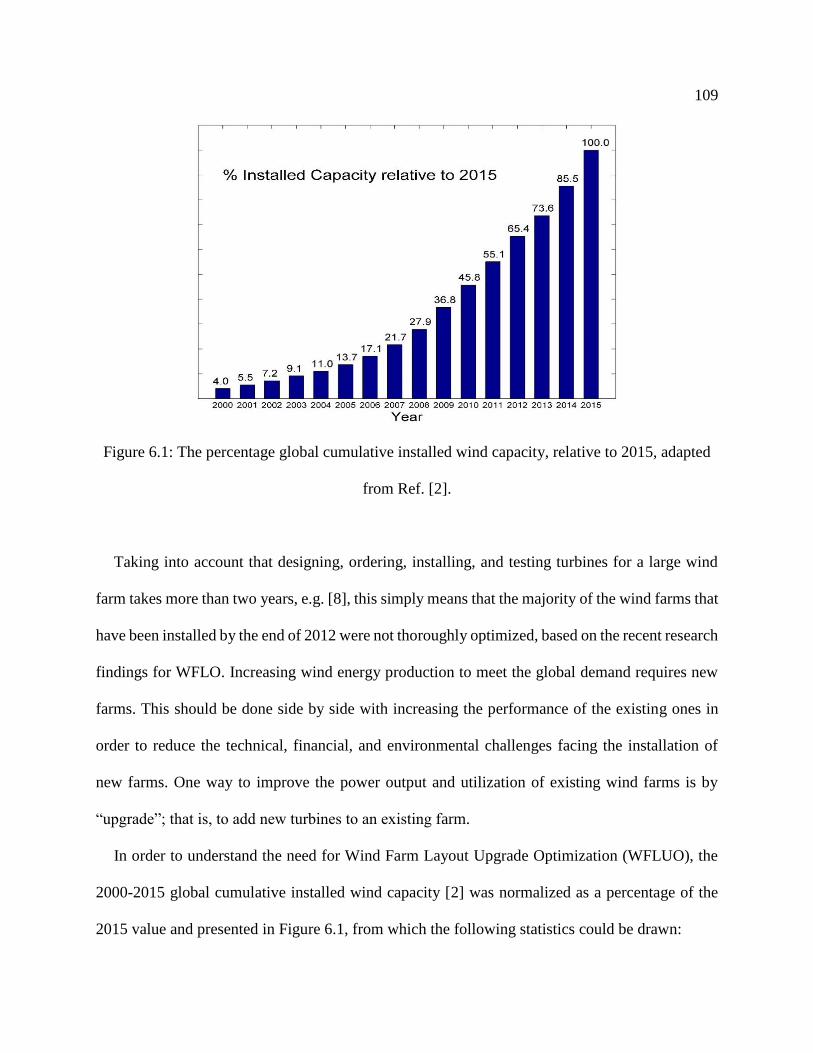
109
Figure 6.1: The percentage global cumulative installed wind capacity, relative to 2015, adapted
from Ref. [2].
Taking into account that designing, ordering, installing, and testing turbines for a large wind
farm takes more than two years, e.g. [8], this simply means that the majority of the wind farms that
have been installed by the end of 2012 were not thoroughly optimized, based on the recent research
findings for WFLO. Increasing wind energy production to meet the global demand requires new
farms. This should be done side by side with increasing the performance of the existing ones in
order to reduce the technical, financial, and environmental challenges facing the installation of
new farms. One way to improve the power output and utilization of existing wind farms is by
“upgrade”; that is, to add new turbines to an existing farm.
In order to understand the need for Wind Farm Layout Upgrade Optimization (WFLUO), the
2000-2015 global cumulative installed wind capacity [2] was normalized as a percentage of the
2015 value and presented in Figure 6.1, from which the following statistics could be drawn:

110
• 96 % of current wind farms were installed during the last 15 years, 86.3 % during the last
decade.
• 65.4 % of the wind farms have been installed by the end of 2012.
The majority of current wind farms may benefit from upgrading, without re-locating or
replacement of the existing turbines as they are in the first half of their lifespan (which is
commonly 20 - 30 years, e.g. [9]).
In this paper, the problem of WFLUO is introduced for the first time in the literature, an upgrade
methodology is proposed and applied to Horns Rev 1 offshore wind farm as a case study. In section
6.2, the case study is highlighted and justified. The proposed upgrade methodology is given in
section 6.3. The results and discussions are the topic of section 6.4, while the most useful
conclusions are listed in section 6.5.
6.2 Horns Rev 1: Background and Reasons for Its Selection
Horns Rev1 is one of the most famous wind farms worldwide. It has received great interest since
commencing power production in 2002 because of many reasons, which can be summarized as:
1. The installed capacity is 160 MW, which made it the world's largest offshore wind farm
when installed and for several years thereafter.
2. Throughout its 13 years of operation it has produced more than 8 TW-hr [10].
3. Three years of detailed wind resource assessment data taken prior to the installation are
publically available [11].
4. Detailed operational measurements are also publically available, e.g. [12].
Accordingly, the farm performance and wake measurements were used in many wake model
validations and wind farm layout optimization studies e.g. [12,13,14,15,16,17,18].

111
Many investigators have computationally improved the Horns Rev 1 performance by relocating
the turbines within the farm area. Rivas, et al. [19] applied the Simulated Annealing Algorithm to
solve the Turbine Positioning Problem in order to maximize the AEP. They concluded that the
AEP could be increased up to 1%. Vezyris [20] applied deterministic, semi-stochastic, and
stochastic approaches in order to minimize the Levelized Production Cost (cents/kWh). The results
showed that a decrease in the Levelized Production Cost by ~1 % combined with an increase in
the AEP with ~1 % could be achieved by re-optimizing the farm layout. Park and Law [21] derived
a continuous and smooth wind speed profile that allowed the wind farm power function to be
expressed as a smooth (differentiable) function of wind turbine location variables. The wind farm
power function then optimized using a gradient-based optimization algorithm. The minimum
turbine proximity was fixed at 5D and the results suggested an increase in the farm output power
by 7.3 %, without providing with any cost calculations.
Horns Rev 1 wind farm is a matrix of 80 identical turbines (8 East to West rows by 10 North to
South columns). The columns are aligned approximately 7.2° West of North, forming a
parallelogram. The turbines are all Vestas V80-2.0 with D = 80 m and 𝑃𝑟 of 2 MW. The spacing
between turbines in both the rows and columns is 7D, as indicated in Figure 6.3. The tower height
is 70 m and the power curve is specific for the turbines delivered to this wind farm and may not
apply to other V80 turbines [12].
Apart from the availability of performance and other data that was noted above, Horns Rev 1
was chosen as a case study as an example of middle-aged non-optimized wind farm, based on the
recent findings. It is slightly more than 13 years old, it contains identical turbines, the turbine 𝑃𝑟
and H are below the recent average values for offshore farms [7], and finally the turbines spacing
is 7D in both directions, which is significantly larger than in more recent farms.

112
The references quoted above optimized the farm performance by computationally re-locating
the turbines, but this is clearly not feasible for most existing wind farms. The present work aims
to give a practical solution for the WFLUO, for the first time in the literature, by not changing the
existing farm layout. The proposed methodology is based on commercial turbine selection and hub
height variation that introduced and tested in [22].
Understanding and analyzing the wind data is an essential task in any wind power project. As
mentioned earlier, three years of wind measurements were made prior to Horns Rev 1 installation.
The wind data at 62 m height from June, 1st, 1999 to May, 31st, 2002 was averaged and Weibull
parameters - scale and shape factors - were evaluated for 12 directional sectors (30 degrees each)
[11]. Moreover, these parameters were extrapolated to the hub height of 70 m [23]. Figure 6.2
shows the frequency of occurrence, f, of each speed (at hub height) at different wind directions in
contour format.
Figure 6.2: Frequency of occurrence, f, of wind speed and direction at hub height for Horns Rev
1, adapted from Ref. [23].

113
6.3 Upgrade Methodology
The proposed upgrade methodology is given in detail in this section. In subsection 3-1, the
proposed upgraded layouts are illustrated. The wake model and wake interference calculations are
described briefly in subsection 3-2. Subsection 3-3 describes the pool commercial turbines from
which were chosen the turbines for the upgraded farm as well as the AEP calculations. The strategy
of hub height variation is discussed in subsection 3-4. Finally, the cost analysis and the
optimization methodology are the topics of subsections 3-5 and 3-6, respectively.
6.3.1 Proposed upgraded layouts.
The development of methodologies for multiple-turbine wind farm layouts (variable turbine size
and/or hub height), e.g. [24,25,26,27,,22], allowed the turbine spacing to be reduced to 3.5D. This
recent finding provides compact farm designs with higher AEP, excellent area and height
utilization, without severe wake loss, and hence lower COE. Accordingly, it was proposed to
install new turbines either inside or outside the existing wind farm area, as illustrated in Figure
6.3a and b, respectively. For the inside upgrade, the farm area was kept unchanged and new
turbines were installed in between the existing ones, in order to maximize the utilization of the
farm space while reducing the added cost due to extra infrastructure. In the outside upgrade, the
added turbines form four rows and four columns outside the existing area, in order to allow larger
turbines to be installed with the least effect on the rest of the turbines. In all cases, Vestas turbines
and the grid layout was considered as this manufacturer’s turbines were used in the original farm.
The number of turbines in the original farm denoted N (N = 80), while the number of the added
turbines denoted M (M = 63 and 68 for the inside and outside layouts, respectively). In all cases,
the existing turbines were numbered from 1 to N, while the added turbines were numbered from

114
N+1 to N+M. The vertical coordinate in Figure 6.3 indicates the North direction and the values in
both vertical and horizontal directions are in terms of D.
(a)
(b)
Figure 6.3: Proposed upgraded layouts for Horns Rev 1 wind farm. (a): inside. (b): outside. The
existing turbines are numbered from 1 to 80 (in black), while the added turbines are numbered
from 81 (in red).

115
As shown in Figure 6.3, the original farm is a parallelogram of base 63D and height 49D which
is unchanged in the inside case. However, the total outside area is a parallelogram of base 91D and
height 77D. Defining the Area Factor, AF, for the upgraded layout as the farm area divided by the
original farm area, gives 𝐴𝐹 for the inside and outside upgrades of 1.0 and 2.27, respectively.
6.3.2 Wake model and interference calculations
Wake modelling is one of the first and most important steps in WFLO. The availability of the field
measurements for some wind farms, especially Horns Rev 1 and Nysted, gave a great opportunity
to validate the existing wake models and even develop new models. Because of many reasons
mentioned in [28,29,30,31], the Jensen wake model was implemented in the present wake
calculation. Ref. [22] demonstrated that the model lead to accurate estimates of the energy
production data for Horns Rev 1 between 2005 and 2015, [31]. Originally proposed by Jensen
[332], the model was developed by Katic et al. [433] and Frandsen [2734]. Full details of its
implementation were given in [22]. Referring to Figure 6.3 and Figure 6.4 [22], the wake
calculations were done as follows:
For each of twelve angles from North, 𝜃 = 0𝑜 , 30𝑜 , 60𝑜 , … , 330𝑜 , the Y-axis used in the
following description was rotated so that the wind was always in the positive Y-direction. The
turbines then sorted in ascending order according to their Y coordinates. For example: the most
upwind turbine, which has the least Y-coordinate, was designated 1, while the most downwind one
was N+M (the total number of turbines). Accordingly, each turbine i in the farm apart from the
most upwind one, 2 < i < N, is potentially affected by the wake of every turbine upwind of it: j, 1
< j < i-1.

116
Figure 6.4: A front view (parallel to wind direction) illustrates the overlap of the upwind turbine
wake (the dashed circle) with the downwind turbine rotor (the solid circle). The Y co-ordinate is
into the page [22].
The roughness length, z0, is an essential parameter in Jensen wake model, on which the vertical
wind profile and the wake entrainment greatly depend. The ambient roughness length for offshore
farms was taken as 0.0002 m in [22] as it widely accepted for open sea, e.g. [35]. However, the
upwind turbines increase the turbulence level within the farm, which in turn increases the effective
roughness. Following many investigators, e.g. [36,37], z0 was taken as 0.05 m in order to match
the field measurement for velocity/power deficits and turbulence level.
The wake analysis used in the present work was described in Ref. [22] and the reader is referred
to that particular reference for full details.
Main
See level
117
6.3.3 Commercial turbines and AEP calculations
In order to obtain practical upgraded layouts, it was decided to restrict the selection to available
models from the same manufacturer as the existing turbines. To this end, the selection in the current
optimization was among 19 Vestas turbines, the turbines were sorted in an ascending order
according to the rated power and then according to the diameter. The turbine code, rated power,
rotor diameter, and rated speed, 𝑈𝑟, are given in Table 6.1.
The manufacturer’s power curves for the 19 turbines were fitted by a 5th degree polynomial and
the coefficients were used to evaluate the power output from any turbine, i, as function of the
effective hub height wind speed, 𝑈𝑖, [22] ahead of its rotor.
Accordingly, the power developed, 𝑃𝑖, by the 𝑖𝑡ℎ turbine based on its type and the effective
wind speed, 𝑈𝑖, was estimated as [22]
𝑃𝑖 = 𝑐𝑖0 + 𝑐𝑖1𝑈𝑖 + 𝑐𝑖2𝑈𝑖2+ 𝑐𝑖3𝑈𝑖
3+ 𝑐𝑖4𝑈𝑖4+ 𝑐𝑖5𝑈𝑖
5 = ∑ 𝑐𝑖𝑘𝑈𝑖𝑘
𝑘=5
𝑘=0
(6.1)
the total farm output power for each wind speed, 𝑣, at each wind direction, 𝜃, is simply the sum
of the individual powers from all turbines
𝑃(𝜃,𝑣) = ∑ 𝑃𝑖
𝑁+𝑀
𝑖=1
= ∑ ∑ 𝑐𝑖𝑘𝑈𝑖𝑘
𝑘=5
𝑘=0
𝑁+𝑀
𝑖=1
(6.2)
and the AEP was calculated as
𝐴𝐸𝑃 = 8,766 ∑ ∑ 𝑓(𝜃,𝑣). 𝑃(𝜃,𝑣)
25
𝑣=4
360
𝜃=0
(6.3)
where 8,766 is the number of hours per year.

118
Turbine code Rated power
(kW)
Rotor diameter
(m)
Rated speed
(m/s)
1 1,815 90 13
2 1,815 100 11.5
3 2,000 80 14
4 2,000 90 13
5 2,000 100 12
6 2,000 110 11
7 2,600 100 15
8 3,000 90 16
9 3,000 112 12
10 3,000 126 10.5
11 3,075 112 13
12 3,300 105 13.5
13 3,300 112 12.5
14 3,300 117 13
15 3,450 105 13.5
16 3,450 112 12.5
17 3,450 117 11.5
18 3,450 126 11.5
19 3,450 136 11
Table 6.1: Code, rated power, rotor diameter, and rated speed for the turbines included in the
selection.

119
6.3.4 Hub height variation
The hub height is one of the most important design parameters for a wind turbine, upon which
power and cost greatly depend. The proper value of H for a specific turbine should consider the
turbine diameter, rated speed, installation cost, wind resources, site restrictions, etc. Moreover,
many recent WFLO studies, e.g. [38,39,22,40], suggest the implementation of individual values
of H for the turbines within the farm, in order to minimize the wake interference, the installation
cost, or a combination of them. In our previous work [22] it was decided to use common H limits
(80 𝑚 ≤ 𝐻 ≤ 140 𝑚) for all turbines. However, in the present work, the investigated range of H
was widened and made flexible (turbine-specific). The Maximum Tip Height (MTH) and the
Minimum Ground Clearance (MGC) along with the turbine diameter were used to determine the
individual H range for each turbine. The MTH and MGC are the blade tip height at its highest and
lowest positions, respectively. The MTH was set as 230 m for Horns Rev wind farms [41], which
matches the world’s tallest installed wind turbine [42]. On the other hand, the recommended value
for the MGC varied worldwide from 5 m to 23 m [35]. However, the rare combination of maximum
wave height and tidal range at Horns Rev site is less than 7 m, the mean value is about 3 m [11].
To this end, the MTH and the MGC were taken as 200 m and 15 m, respectively. Accordingly, the
individual turbine’s H limits and Hub Height Range (HHR) for any turbine, 𝑖, based on its rotor
diameter, 𝐷𝑖, as
𝐻𝑚𝑎𝑥,𝑖 = 𝑀𝑇𝐻 − (𝐷𝑖
2) (6.4)
𝐻𝑚𝑖𝑛,𝑖 = 𝑀𝐺𝐶 + (𝐷𝑖
2) (6.5)
𝐻𝐻𝑅𝑖 = 𝐻𝑚𝑎𝑥,𝑖 − 𝐻𝑚𝑖𝑛,𝑖 (6.6)

120
Figure 6.5 shows 𝐻𝑚𝑎𝑥, 𝐻𝑚𝑖𝑛, and HHR as function of D in the investigated range (80 𝑚 ≤
𝐷 ≤ 136 𝑚), as given in Table 6.1.
Figure 6.5: Hmax, Hmax, and HHR as function of D in the investigated range.
6.3.5 Modified simple cost model
The cost model used in this study is a modified version of the simple model introduced in detail in
[22]. Only the major assumptions for offshore conditions along with the modifications that made
based on the most recent cost reports, e.g. [44] will be given in this subsection.
1. The Total Cost of a wind farm is a combination of the Capital Cost, Cc and the Operation
and Maintenance cost, O&M, CO&M. It was assumed that 𝐶𝐶 = 0.75, while 𝐶𝑂&𝑀 = 0.25.
2. The CC in turn is subdivided into the total turbine cost, 𝐶𝑡𝑢𝑟𝑏𝑖𝑛𝑒, = 0.329𝐶𝐶, and the
remainder, 0.671𝐶𝐶, is the Financial & Balance of system costs, 𝐶𝐹&𝐵.
3. The tower cost, 𝐶𝑡𝑜𝑤𝑒𝑟, is about 0.1831 of the 𝐶𝑡𝑢𝑟𝑏𝑖𝑛𝑒, or 0.06 of the 𝐶𝐶.

121
4. The 𝐶𝐹&𝐵 depends only on the farm area. In other words, if the turbines were added within
the original farm area, the added 𝐶𝐶 would comprise only 𝐶𝑡𝑢𝑟𝑏𝑖𝑛𝑒 while 𝐶𝐹&𝐵 were
considered unchanged.
5. The cost of 1.0 MW at the corresponding 𝐻𝑚𝑖𝑛 was taken as the unit cost and was denoted
by Unit Cost Index, UCI. The corresponding capital and total costs were denoted Capital
Cost Index, CCI, and Total Cost Index, TCI, respectively. Each 1 m increase of 𝐻𝑖 over
𝐻𝑚𝑖𝑛,𝑖 was assumed to add 𝐶𝑡𝑜𝑤𝑒𝑟
𝐻𝑚𝑖𝑛,𝑖 to the CCI.
Accordingly, the added TCI as a result of the upgrade can be expressed as
𝑇𝐶𝐼𝑎 =𝐴𝐹
(1 − 𝐶𝑂&𝑀)(1 − 𝐶𝑡𝑢𝑟𝑏𝑖𝑛𝑒)∑ 𝑃𝑟,𝑖 [1 +
𝐶𝑡𝑜𝑤𝑒𝑟
𝐻𝑚𝑖𝑛,𝑖(𝐻𝑖 − 𝐻𝑚𝑖𝑛,𝑖)]
𝑀
𝑖=1
(6.7)
where 𝑃𝑟,𝑖 and 𝐻𝑖 are the rated power (in MW) and the hub height (in m) of the 𝑖𝑡ℎ turbine,
respectively, while 𝐴𝐹 is the Area Factor as introduced in subsection 3-1.
Based on the above analysis, the TCI for the original farm, 𝑇𝐶𝐼𝑂 is
𝑇𝐶𝐼𝑂 =1.0
(1 − 0.25)(1 − 0.329)∑ 2.0 [1 +
0.06
55(70 − 55)]
80
𝑖=1
= 323 𝑈𝐶𝐼 (6.8)
Two useful quantities are defined; the Cost Of Added Energy Index (COAEI) and the Cost Of
Total Energy Index (COTEI):
𝐶𝑂𝐴𝐸𝐼 =𝑇𝐶𝐼 𝑎
𝐴𝐸𝑃 − 𝐴𝐸𝑃𝑂 (6.9)
𝐶𝑂𝑇𝐸𝐼 =𝑇𝐶𝐼 𝑎
𝐴𝐸𝑃 (6.10)
where 𝐴𝐸𝑃𝑂 = 715 MW-hr is the estimated AEP for the original farm.
Finally, the three objective functions considered in the optimization are shown in Table 6.2.

122
ObjFun# Optimizer Equation
ObjFun1 max AEP (6.3)
ObjFun2 min COAEI (6.9)
ObjFun3 min COTEI (6.10)
Table 6.2: Illustration of the three objective functions.
6.3.6 Optimization
Layout optimization for large wind farms with commercial turbine selection is one of the most
complex optimization problems because it is discrete, non-convex, non-linear, and of high
dimension. Genetic Algorithms (GA) are one of the most successful optimization methods for such
problems that their capability has been proven over years, especially with WFLO, e.g. [45]. On
the other hand, GA is slow compared with other optimization methods [45,46] as it depends
basically on successive random search. The solution evolves from one generation of a fixed
population size (PS) to the next generation. In general, the larger the PS the wider the search and
the greater the probability of finding the global optima. On the other hand, very large PS requires
large execution time and may disperse the conversion to the global optima, e.g. [47,48]. In general,
the CPU time is nonlinear in PS and the proper choice of PS is greatly problem dependent.
However, a simple test case from the current work showed that an increase in PS from 15 to 45
(300%) the execution time increased by about 390% (this relative increase would increase if PS
were increased from 45 to 135 for example). Accordingly, it is very important to select the proper
PS in order to increase the probability of finding the global optima while keeping the execution
time reasonable, e.g. [49].

123
For both inside and outside layouts, two cases were investigated. Single turbine with variable
H was the first with only ObjFun1. Multi-turbine with variable H and the three objective functions
were then considered in turn.
Two significant modifications were made compared to what described in Ref. [22]. First, the
H variation was treated for each turbine individually based on its D. Accordingly, the upper and
lower bands for H were not the same for all turbines and the individual height was not included
explicitly in the optimization design variables. Instead, a fractional parameter denoted “coefficient
of height” was an optimization design variable with the same upper and lower bands (1.0 and 0.0,
respectively) for all turbines. Once the coefficient of height, 𝐶𝐻, is selected (during the
optimization) for a particular turbine, 𝑖, the corresponding value of 𝐻𝑖 is calculated using Equation
(6) as
𝐻𝑖 = 𝐻𝑚𝑖𝑛,𝑖 + 𝐶𝐻. 𝐻𝐻𝑅𝑖 (6.11)
Second, as discussed earlier in this subsection, as the PS increases the execution time per
generation increases significantly. A global optimization technique called “Random Independent
Multi-Population Genetic Algorithm, RIM-GA” was applied to the GA used for the multi-turbine
cases, as it has double the variables than the single turbine cases. The multi-population genetic
algorithms (in general) have been proven as a powerful tool to enhance the GA optimization
efficiency, e.g. [50]. An arbitrary number of independent populations, 𝑛, having relatively small
population size, 𝑝𝑠, were initiated and allowed to evolve over a small number of generations, 𝑔1.
The final population from each run was stored, sorted based on the ObjFun value. The fittest 𝑚
individuals from each independent run were collected and assigned as the initial population for
one last run for 𝑔2 generations. Again, the effectiveness of this technique is problem dependent,
however, RIM -GA was tested with some test cases and gave almost the same results but with 82

124
- 87 % of the execution time. The comparison was made against single runs having population size
𝑃𝑆 = 𝑚. 𝑛. 𝑝𝑠 and number of generations, 𝐺 = 𝑔1 + 𝑔2.
6.4 Results and Discussion
Two proposed upgraded layouts (inside and outside) were investigated. The existing 80 turbines
were left unchanged, while suitable locations were specified for the new turbines. The selection
was among 19 Vestas commercial turbines covering a rated power range of 1.8 – 3.45 MW and
rotor diameter range from 80 – 136 m. MATLAB’s genetic algorithm solver, ga, was employed
for the optimization and three objective functions in Table 6.2 were considered individually.
AEP and the TCI were normalized with respect to the corresponding values for the original
farm (AEPO and TCIO, respectively), the two normalized quantities were denoted NAEP and
NTCI, respectively. Moreover, the NTCI were divided by the NAEP, the resulted quantity called
Normalized Cost Of Energy Index, NCOEI.
Figure 6.6 shows the NAEP, NTCI, and NCOEI for the single turbine cases and ObjFun1. In
these cases, the M added turbines were assumed identical in type, but different in height. The major
remarks are summarized below:
1. There is a wide range of feasible optimum upgrades providing a useful trade-off between
AEP and COE.
2. The single turbine inside layouts produce a range of NAEP from 1.90 to 2.60 with a NTCI
from 1.47 to 2.87, based on the turbine model and optimization objective.
3. The single turbine outside layouts gave NAEP from 2.23 to 3.36 with a NTCI from 3.81 to
7.20, based on the turbine model and optimization objective.

125
4. The inside layout produces a cheap added AEP if small turbines are used. The added AEP
increases as the turbine size increases, but at a higher rate in the added cost. The reason is
the limited wind resources which causes the increase in AEP to reduce as the turbine size
(and hence the cost) increases.
5. As expected, the outside layout adds more AEP than the inside one, however, this increase
in AEP is accompanied with very high cost as a consequence of adding area to the farm.
6. Both inside and outside layouts have the same trends in AEP and TCI (qualitatively),
however, the latter has magnified scales, especially for the cost.
7. Both layouts confirm the superiority of using turbines with relatively large D and relatively
low 𝑈𝑟 (turbines number 2, 1, 6, 5, 4, and 3) than the opposite (turbines number 15, 8, 17,
16, and 12). This finding matches with that obtained in the previous research [22] and with
others in the literature, e.g. [51].
8. The NCOEI for the inside layouts are usually close to unity, which means that the increase
in added AEP coincides with a comparable increase in the TCI.
As the turbine type was fixed in these cases, the hub height variation (not presented here for the
sake of brevity) plays the main role in both AEP maximization and COE minimization. For the
max AEP optimization, the majority of turbines should be installed as high as possible in order to
meet the highest possible wind speed, while the minimum height was required for the rest of
turbines, especially in the middle of the farm, in order to allow wake recovery ahead of the exterior
turbines.
For the min COE optimizations, heights close to 𝐻𝑚𝑖𝑛 were dominant, and scattered values
close to 𝐻𝑚𝑎𝑥 were selected in order to capture the most power at a few locations and to allow

126
wake recovery for the rest of the turbines at lower heights in order to reduce the COE. In general,
a wide range of H was used in order to compensate the absence of the turbine selection.
(a)
(b)
Figure 6.6: Normalized AEP, TCI, and COEI for single turbine layouts.

127
Figure 6.7 shows the NAEP, NTCI, and NCOEI for the multi-turbine layouts where the M added
turbines could be different in both type and height. The rated power distribution for the selected
turbines and the corresponding coefficient of height distribution are given in Figure 6.8 and Figure
6.9, respectively. In Figures 8 to 11, symbols (I) and (O) represent the inside and the outside
layouts, respectively, while the number indicates the ObjFun# as given in Table 6.2. For example:
I2 represents the Inside layout with ObjFun2.
Finally, the histogram of turbine and 𝐶𝐻 selection frequencies for all multi-turbines cases are
given in Figure 6.10 and Figure 6.11, respectively. Again, the outside layout gives significant more
AEP but with a huge cost (Figure 6.7) because of the added area (and hence 𝐶𝐹&𝐵) compared to
the inside layout. The optimization for max AEP (ObjFun1) gave results close to those for the
single-turbine case of larger size for both inside and outside layouts. This can be explained by the
turbine selection distribution (Figure 6.8) which shows for maximum AEP regardless the cost,
larger turbines should be used as much as possible. The resulting layouts usually have high total
cost and COE. Similarly, but at the other extreme, the optimization for min COTEI (ObjFun3)
gave results close to those for the single-turbine case of smaller size in both inside and outside
layouts. This can be also explained by the turbine selection distribution (Figure 6.8) which shows
for maximum COE, the selection should be among small size turbines in general. The larger
turbines should be selected carefully in some places where the increase in power output dominates
the corresponding increase in cost. The medium size turbines were rarely used, which means that
the proper turbine selection should be, in general, among a few large turbines and a few small
ones. The optimization for max AEP requires significantly wider range in both turbine size and H.
On the other hand, the optimization for min COE requires a much smaller range of both turbine
size and H.

128
(a)
(b)
Figure 6.7: Normalized AEP, TCI, and COEI for multi-turbine layouts.

129
Figure 6.8: Rated power distribution for the selected turbines for all multi-turbine cases.
Figure 6.9: Coefficient of height, CH, distribution for all multi-turbine cases.

130
Figure 6.10: Frequency of turbine selection for multi-turbine cases.
Figure 6.11: Frequency of CH selection for multi-turbine cases, with bin width = 0.05.

131
6.5 Conclusions
In this paper, the large wind farm layout upgrade optimization problem was introduced. The
proposed upgrade methodology was based on adding new non-identical turbines to the existing
farm either within the farm area or as an extension. The famous Horns Rev 1 large offshore wind
farm was taken as a case study. The existing 80 turbines were kept as they are while 63 and 88
turbines were added in the inside and outside upgraded layouts, respectively. 19 Vestas
commercial turbines of rated power raged from 1.8 to 3.45 MW were included in the selection.
The following are the implications of the findings of this paper:
1. Existing wind farms can be effectively upgraded by increasing the energy production by
adding new turbines, while keeping the existing turbines unchanged.
2. Wind farm layout upgrade optimization for offshore farms is recommended if it is done
within the original farm area and infrastructure. In this case, a significant increase in the
energy production can be achieved while keeping the cost of energy in reasonable range.
3. Wind farm layout upgrade optimization is an efficient method to increase the utilization of
the existing area instead of installing new costly farm(s).
4. Having a range of commercial turbines for selection as well as allowing variation in height
is a powerful tool in wind farm layout upgrade optimization.
5. The optimum layouts are greatly dependent on the proposed upgraded layout as well as the
optimization objective.
6. The hub height variation is beneficial not only to reduce the wake interference and hence
increase the energy production, but also to reduce the total cost as well as the cost of energy.

132
7. By including a wide range of commercial turbines in the selection, a wide band of feasible
optimum layouts is obtained which provide a trade-off between energy production and cost.
8. Among commercial turbines having the same rated power, the priority in selection should
be biased towards the turbines with larger diameter and lower rated speed.
9. The random independent multi-population technique reduces the execution time for the
genetic algorithm without compromising the outcomes.
ACKNOWLEDGEMENTS
This research is part of a program of work on renewable energy funded by the Natural Science and
Engineering Council (NSERC) and the ENMAX Corporation. The first author also acknowledges
the Egyptian Government and Prof. El-Adl El-Kady for support and supervision during the early
(and the important) part of this work.

133
6.6 References
1. REN21. 2016. Renewables 2016 Global Status Report (Paris: REN21 Secretariat). ISBN
978-3-9818107-0-7.
http://www.ren21.net/wp-content/uploads/2016/06/GSR_2016_Full_Report.pdf [last
accessed: July 2017].
2. Global wind report, Annual market update 2015, Global Wind Energy Council (GWEC),
April, 2016.
3. http://www.tsp-data-portal.org/Breakdown-of-Electricity-Capacity-by-Energy-
Source#tspQvChart [last accessed: July 2017].
4. http://www.tsp-data-portal.org/Breakdown-of-Electricity-Generation-by-Energy-
Source#tspQvChart [last accessed: July 2017].
5. http://www.ucsusa.org/clean_energy/our-energy-choices/renewable-
energy/environmental-impacts-wind-power.html#references [last accessed: July 2017].
6. Mosetti, G., Poloni, C., Diviacco, B. (1994). Optimization of wind turbine positioning in
large wind farms by means of a genetic algorithm. Journal of Wind Engineering and
Industrial Aerodynamics, 51, pp. 105-116.
7. 2014 Wind technologies market report highlights. Prepared for US Department of Energy,
Wind and Water Power Technologies Office (Berkeley, CA: August 2015)
8. Lindvig, K. (2010). European forum for renewable energy sources the installation and
servicing of offshore wind farms. CSO, A2SEA A/S 16th September 2010.
9. http://www.ewea.org/wind-energy-basics/faq/ [last accessed: July 2017].
10. http://www.ens.dk/node/2233/register-wind-turbines [lase accessed: July 2017].

134
11. Sommer, A., Hansen, K., (2002). Wind resources at Horns Rev, Tech-Wise A/S, Eltra
PSO-2000 Proj. NR. EG-05 3248, Report no. D-160949, Project no. 11746.01.06, p. 69.
12. Jensen, L., Mørch, C., Sørensen, P., Svendsen, K. H. (2004). Wake measurements from the
Horns Rev wind farm, EWEC 2004, 22-25, London, United Kingdom.
13. Barthelmie, RJ, Hansen, K, Frandsen, ST, Rathmann, O, Schepers, JG, Schlez, W, Phillips,
J, Rados, K, Zervos, A, Politis, ES, Chaviaropoulos, PK. (2009). Modelling and measuring
flow and wind turbine wakes in large wind farms offshore. Wind Energy 2009, 12, pp.
431–444.
14. Rathmann, O, Barthelmie, RJ, Frandsen, ST. (2006). Wind turbine wake model for wind
farm power production, European Wind Energy Conference, Athens.
15. Barthelmie, RJ, Pryor, S, Frandsen, ST, Hansen, KS, Schepers, JG, Rados, K, Schlez, W,
Neubert, A, Jensen, LE, Neckelmann, S. (2010). Quantifying the impact of wind turbine
wakes on power output at offshore wind farms. Journal of Atmospheric and Oceanic
Technology, 27, pp. 1302-1317.
16. Frandsen, S, Barthelmie, R, Pryor, S, Rathmann, O, Larsen, S, Højstrup, J, Thøgersen, M.
(2006). Analytical modelling of wind speed deficit in large offshore wind farms. Wind
Energy, 9, pp. 39–53.
17. Frandsen, S, Rathmann, O, Barthelmie, R, Jørgensen, HE, Badger, J, Hansen, K, Ott, S,
Rethore, P, Larsen, SE, Jensen, LE. (2008). The making of a 2nd generation wind farm
model. Wake Meeting, Dong Energy, Copenhagen.
18. Beaucage, P., Robinson, N., Brower, M., Alonge, C. (2012). Overview of six commercial
and research wake models for large offshore wind farms, EWEA Proceedings, 10 p.,
Copenhagen, Germany.

135
19. Rivas, R., Clausen, J., Hansen, K., Jensen, L., (2009). Solving the turbine positioning
problem for large offshore wind farms by simulated annealing. Wind Engineering, 33(3),
pp. 287-297.
20. Vezyris, C. (2012). Offshore wind farm optimization investigation of unconventional and
random layouts. MSc Thesis, TU Delft, Netherlands.
21. Park, J., Law, K. (2015). Layout optimization for maximizing wind farm power production
using sequential convex programming. Applied Energy, 151, pp. 320–334.
22. Abdulrahman, M, Wood, D. (2017). Investigating the power-COE trade-off for wind farm
layout optimization considering commercial turbine selection and hub height variation.
Renewable Energy, 102(B), pp. 267-516.
23. Feng, Ju, and Wen Zhong Shen. (2015). Modelling wind for wind farm layout optimization
using joint distribution of wind speed and wind direction. Energies 8.4, pp. 3075-3092.
24. Herbert-Acero, J-F., Franco-Acevedo, J-R., Valenzuela-Rendon, M., Probst-Oleszewski,
O. (2009). Linear wind farm layout optimization through computational intelligence.
Proceedings of 8th Mexican International Conference on Artificial Intelligence, pp. 692–
703.
25. Tesauro, A., Réthoré, P-E, Larsen, G.C. (2012). State of the art of wind farm optimization.
Proceedings of European Wind Energy Conference & Exhibition, European Wind Energy
Association (EWEA 2012), Copenhagen, Denmark.
26. Chowdhury, S., Zhang, J., Messac, A., Castillo, L. (2013). Optimizing the arrangement and
the selection of turbines for wind farms subject to varying wind conditions. Renewable
Energy, 52, pp. 273-282.

136
27. Chen, Y., Li, H., Jin, K., Song, Q. (2013). Wind farm layout optimization using genetic
algorithm with different hub height wind turbines. Energy Conversion and Management,
70, pp. 56–65.
28. Sørensen, T., Nielsen, P., Thøgersen, M.L. (2006). Recalibrating wind turbine wake model
parameters – Validating the wake model performance for large offshore wind farms. EMD
International A/S.
29. Sørensen, T., Thøgersen, M.L., Nielsen, P., Jernesvej, N. (2008). Adapting and calibration
of existing wake models to meet the conditions inside offshore wind farms. EMD
International A/S.
30. Barthelmie, R.J., Folkerts, L., Larsen, G.C., Rados, K., Pryor, S.C., Frandsen, S.T., Lange,
B., Schepers, G. (2006). Comparison of wake model simulations with offshore wind
turbine wake profiles measured by SODAR. Journal of Atmospheric & Oceanic
Technology, 23(7), pp. 888-901.
31. Beaucage, P., Robinson, N., Brower, M., Alonge, C. (2012). Overview of six commercial
and research wake models for large offshore wind farms. Proceedings of the EWEA
conference, Copenhagen.
32. Jensen, N.O. (1983). A note on wind generator interaction. Risø-M-2411, Risø National
Laboratory.
33. Katic, I., Hojstrup, J., Jensen, N.O. (1986). A simple model for cluster efficiency. In
Proceedings of the European Wind Energy Association Conference and Exhibition, pp.
407–410.
34. Frandsen, S. (1992). On the wind speed reduction in the center of large clusters of wind
turbines. Journal of Wind Engineering and Industrial Aerodynamics, 39, pp. 251-265.

137
35. Wieringa, J. (1992). Updating the davenport roughness classification. Journal of Wind
Engineering and Industrial Aerodynamics, 41, pp. 357-368.
36. Port-Agel F, Wu Y-T, Chen C-H. (2013). A numerical study of the effects of wind direction
on turbine wakes and power losses in a large wind farm. Energies, 6(10), pp. 5297–5313
37. Jensen, L., Wake losses and turbulence within the Horns Rev off-shore wind farm. Elsam
Engineering A/S.
https://www.ieawind.org/task_23/Subtask_1S_docs/PPT_Risoe1205/Jensen.pdf [lase
accessed: July 2017].
38. Chowdhury, S., Zhang, J., Messac, A., Castillo, L. (2013). Optimizing the arrangement and
the selection of turbines for wind farms subject to varying wind conditions. Renewable
Energy, 52, pp. 273-282.
39. Chen, Y., Li, H., Jin, K., Song, Q. (2013). Wind farm layout optimization using genetic
algorithm with different hub height wind turbines. Energy Conversion and Management,
70, pp. 56-65.
40. Chen, K., Song, M.X., Zhang, X., Wang, S.F. (2016). Wind turbine layout optimization
with multiple hub height wind turbines using greedy algorithm. Renewable Energy, 96 (A),
pp. 676- 686.
41. Horns Rev 3 - Technical project description for the large-scale offshore wind farm (400
MW) at Horns Rev 3. ENERGINET, Document no. 13/93461-2897, dated 28.04.2014.
42. http://www.nordex-online.com/en/news-press/news-
detail.html?tx_ttnews%5Btt_news%5D=2772&cHash=5f3689a99a [lase accessed: July
2017].

138
43. Oteri, F. (2008). An overview of existing wind energy ordinances. National Renewable
Energy Laboratory Technical Report, NREL/TP-500-44439.
44. Christopher Moné, Tyler Stehly, Ben Maples, and Edward Settle, (2015). 2014 Cost of
wind energy review. National Renewable Energy Laboratory (NREL).
45. Samorani, M. (2010). The wind farm layout optimization problem. Technical Report,
Leeds School of Business, University of Colorado.
46. Tesauro, A., Réthoré, P-E, Larsen, G.C. (2012). State of the art of wind farm optimization.
Proceedings of European Wind Energy Conference & Exhibition, European Wind Energy
Association (EWEA 2012), Copenhagen, Denmark.
47. Goldberg, D.E. (1989b). Sizing populations for serial and parallel genetic algorithms.
Proceedings of the Third International Conference on Genetic Algorithms, San Mateo, CA:
Morgan Kaufman. pp. 70-79.
48. Deb, K., Agrawal, S. (1999). Understanding interactions among genetic algorithm
parameters. Foundations of Genetic Algorithms V, San Mateo, CA: Morgan Kauffman, pp.
265–286.
49. Gotshall, S., Rylander, B. (2003). Optimal population size and the genetic algorithm.
School of Engineering University of Portland, USA.
50. Kim, J. O. (1992). A multi-population genetic algorithm and its application to design of
manipulators. In Proc. IEEE/RSJ Int. Conf. on Intelligent Robots and Systems, Raleigh,
NC, 1992 (pp. 279-286).
51. Rehman, S., Khan, S. A. (2016). Fuzzy logic based multi-criteria wind turbine selection
strategy - A case study of Qassim, Saudi Arabia, Energies 2016, 9, 872.

139
Chapter 7 : Conclusions and Suggestions for Further Investigations
7.1 Introduction
The thesis was organized in such a way to reflect both logical order and research time frame. In
this chapter, the research sequence is illustrated, the chapters are connected, and the findings from
the different papers are integrated. Finally, some further investigations are suggested.
7.2 Findings from “Explicit Solutions for Simple Models of Wind Turbine Interference”
In this paper, the selfish and co-operative optimization strategies were investigated analytically.
The severe wake interference case of N turbines in-line with the wind was considered. The turbines
were assumed identical and the design variable was the axial induction factor, 𝑎. Three simple
models for output power optimization were applied, individually. The first model was with no
wake recovery, the second model was an extension of the first model with including a simple wake
recovery factor, 𝑏 (𝑏 = 1 corresponds to no wake recovery, while 𝑏 = 0 results in complete wake
recovery). Topographical effects were included in the third model by allowing the wind speed at
the second and subsequent turbines to vary by a factor 𝑘 from the reference value at the first
turbine.
The major outcome from this paper is the superiority of the co-operative optimization over
the selfish (individual) one in all cases considered. The formal proof of this result for simple wake
models is the first in the open literature. In other words; the upstream turbine(s) should not capture
the maximum possible energy from the wind. Instead, more energetic wind should be left for the
downstream turbines to increase the total power output. It was also proven that the degree of

140
performance reduction for the upstream turbine(s) increases as the number of turbines in the line
increases and/or the turbines’ proximity decreases.
The next step(s) were to examine these findings from analytic solutions of simple models on
more realistic cases. i.e. real turbines, accurate wake model, and/or real wind farms.
7.3 Findings from “Some Effects of Efficiency on Wind Turbine Interference and Maximum
Power Production”
The performance of the commercial turbines was compared with the actuator disk model (as a
theoretical limit). Accordingly, new operational efficiencies (aerodynamic, conversion, and
overall efficiencies) were defined. It was decided to investigate the effect of the turbine
aerodynamic efficiency on the power production for both selfish and co-operative power
maximization. All calculations were done for six turbines in line at spacing of 4, 5, and 6 rotor
diameters on the grounds, as these were representative values. The classical Jensen’s wake model
was implemented and the turbines’ performance was judged by the power coefficient and the blade
axial induction factor. MATLAB’s genetic algorithm solver, ga, was used to perform the
optimization for the co-operative cases. On the other hand, selfish control was computed by
adapting all the N turbines to work at the maximum possible individual power coefficient.
The results confirmed the superiority of the co-operative optimization over the selfish one. The
difference between the two optimization strategies was found to increase as the turbines’
efficiencies increase and/or the turbine spacing decreases.
The outcome from the first two papers has led to the fact that the operation of each turbine
within the farm should be adapted (based on its location) to increase the total power. Thus, the
non-identical turbine selection for wind farms was found to be more suitable than the classical use

141
of identical turbines. For example: it is more economical to install small turbines somewhere in
the farm instead of installing larger (and hence more expensive) turbine while operating at very
low power coefficient as suggested by the co-operative optimization.
Accordingly, it was decided to proceed for the next step by including co-operative optimization
for non-identical turbines (different models with variable hub height).
7.4 Findings from “Investigating the Power-COE Trade-Off for Wind Farm Layout
Optimization Considering Commercial Turbine Selection and Hub Height Variation”
The commercial turbine selection was added to the wind farm layout optimization problem for the
first time. Generic realistic representation for the thrust coefficient in terms of the power
coefficient were developed from the available commercial turbines’ data. Hub height variation and
three optimization objectives (implemented individually) were also considered. Field-based cost
model was developed to estimate the cost of the different layouts for both onshore and offshore
conditions. Simple wind conditions and simple test cases were considered in order to investigate
the effect of the turbine selection, hub height variation, and optimization objective on the optimal
layouts.
The results showed strong reasons to suggest that wind farm design with identical turbines
should be abandoned in favour of using a range of commercial turbines and hub heights. The
resulted optimum layouts showed a wide range of power-cost of energy trade-off. Almost all the
61 turbines were selected at least once in one optimum layout. However, the priority in selection
was biased towards the larger diameter combined with lower rated speed, followed in order by
larger diameter with higher rated speed, the smaller diameter with lower rated speed, and finally

142
the smaller diameter combined with higher rated speed. The optimization was found more effective
in offshore wind farms because of the low entrainment which delays the wake recovery.
It was decided to apply the previous research findings to a real case study. Instead of re-
optimizing an existing wind farm, it was decided to investigate the upgrade possibilities while
keeping the existing turbines. Finally, the offshore farms were preferred as it was found that the
optimization is more efficient at such conditions.
7.5 Findings from “Large Wind Farm Layout Upgrade Optimization”
In this paper, the large wind farm layout upgrade optimization problem was introduced. It has not
been studied previously in the literature. The proposed upgrade methodology was based on adding
new and different turbines to the existing farm either within the farm area or as an extension. The
famous Horns Rev 1 large offshore wind farm was taken as a case study. The existing 80 turbines
were kept as they are while 63 and 88 turbines were added inside and outside the original farm
area, respectively. Nineteen Vestas commercial turbines of rated power raged from 1.8 to 3.45
MW were included in the selection. The following remarks summarize the output from this paper:
1. Existing wind farms can be effectively upgraded by increasing the energy production by
adding new turbines, while keeping the existing turbines unchanged.
2. Wind farm layout upgrade optimization for offshore farms is recommended if it is done
within the original farm area and infrastructure. In this case, a significant increase in the
energy production can be added while keeping the cost of energy in reasonable range.
3. Wind farm layout upgrade optimization is an efficient solution to increase the utilization
of the existing area instead of installing new costly farm(s).

143
4. Having a range of commercial turbines for selection as well as allowing variation in height
is believed to be a powerful tool in wind farm layout upgrade optimization.
5. The resulted optimum layouts are greatly dependent on the proposed upgraded layout as
well as the optimization objective.
6. The hub height variation is beneficial not only to reduce the wake interference and hence
increase the energy production, but also to reduce the total cost as well as the cost of energy.
7. By including a wide range of commercial turbines in the selection, a wide band of feasible
optimum layouts is obtained which provide a trade-off between energy production and cost.
8. Among commercial turbines having the same rated power, the priority in selection should
be biased towards the turbines with larger diameter and lower rated speed.
9. The random independent multi-population technique reduces the execution time for the
genetic algorithm without compromising the outcomes.
Subsequent to submitting Chapter 6 for publication, a formula was developed including the
turbine technical data given in Table 6.1 to represent the resulted NCOEI (Figure 6.6b). The best
fit, shown in Figure 7.1, was denoted Turbine COE Comparison Index (TCCI)
𝑇𝐶𝐶𝐼 = 𝑃𝑟
0.783
𝐷0.527 (7.1)
Equation (7.1) has a maximum local deviation of 5.5 %. This formula should play an important
role in comparing two or more turbines from the COE point of view. It is clear from Equation (7.1)
that the turbine diameter has an important inverse effect while the rated power is dominant. The
effect of the rated speed was found to be negligible, the reason is believed to be the relatively high
wind speeds considered in the present work.

144
Figure 7.1: TCCI vs NCOEI.
Moreover, Figure 7.2 shows the dependence of TCCI on 𝑃𝑟 and 𝐷 according to Equation (7.1),
within the investigated ranges. Beside the opposite effects of 𝑃𝑟 and 𝐷 on TCCI, Figure 7.2 also
predicts that the use of large diameter is crucial for turbines with high rated power.
Figure 7.2: TCCI dependence on Pr and D.
145
7.6 Suggestions for Further Investigations
The present research used classical models of wind turbine wake, along with some simplified
installations, i.e. offshore as they do not have complex topography, and some complex parameters
were ignored. The following suggestions for further investigations address some of these issues:
1. The study of onshore sites with complex terrain, and hence more complex spatial variations
in the wind speed.
2. Further improvement to the optimization performance for WFLO, either by GA or by
considering new powerful optimization techniques.
3. Using different turbines and hub heights in the farm layout significantly increases the
contribution of partial wake interference, which is believed to increase the dynamic loading
on the rotor. The minimization of dynamic loading is suggested as a new aspect to WFLO.
4. For very large farms, the effect of wake meandering and yaw alignment delay on the energy
production are suggested to be considered.
5. Continuous improvements on cost analysis is suggested in order to be more accurate while
being simple and general. One area on which very little information was available was the
dependence of tower cost on height. Improved estimates for this would be valuable given
the demonstration of the importance of varying this height.
6. The collaboration between WFLO and Co-operative control is believed to be possible and
beneficial. In other words, future WFLO should consider more than just turbine siting.
![The Wind Farm Layout Optimization Problem - Semantic … · In the first case, ... In their survey of these studies, Vermeer et al. [13] ... The Wind Farm Layout Optimization Problem](https://img.dokumen.tips/doc/110x75/5af19fc57f8b9aa9168f5751/the-wind-farm-layout-optimization-problem-semantic-the-rst-case-in.jpg)