Embed Size (px)
Citation preview
1
WIND ENERGY UTILIZATION IN ARCTIC CLIMATE – RACMO 2.3
GREENLAND CLIMATE RUNS PROJECT
Dissertation in partial fulfillment of the requirements for the degree of
MASTER OF SCIENCE WITH A MAJOR IN ENERGY TECHNOLOGY WITH
FOCUS ON WIND POWER
Uppsala University
Department of Earth Sciences, Campus Gotland
José Pedro da Silva Soares
8th
November of 2016

2
WIND ENERGY UTILIZATION IN ARTIC CLIMATE – RACMO 2.3 GREENLAND
CLIMATE RUNS PROJECT
Dissertation in partial fulfillment of the requirements for the degree of
MASTER OF SCIENCE WITH A MAJOR IN ENERGY TECHNOLOGY WITH
FOCUS ON WIND POWER
Uppsala University
Department of Earth Sciences, Campus Gotland
Approved by:
Supervisor, Simon-Philippe Breton
Examiner, Jens Nørkær Sørensen
8th
November of 2016

iii
iii
ABSTRACT
The potential for wind power development in Greenland is evaluated based on the
analysis of 58 years of data (1957-2015) from RACMO 2.3 (Regional Atmospheric
Climate Model). In order to create a wind power development tool, mesoscale maps
based on RACMO 2.3 model were created containing the following characteristics:
mean wind speeds (at 10 m), averaged maximum wind speed (with and without gusts at
10 m), temperature, humidity, geopotential, ice sheet mask and land sheet mask. A
relevant aspect for this thesis is the mean wind speed. Over Greenland, the lower mean
wind speeds range from 2-3 m/s on the tundra areas near the coast. This is influenced by
high temperature inversion over the arctic tundra which disintegrates the predominant
katabatic flow leading to lower wind speeds. On the other hand, the highest mean wind
speeds range from 6 to 10 m/s and are observed in the northeastern region, due to
cyclonic activity over the Greenland Sea. Maps of both the mean wind speed and
averaged maximum wind speed are combined in order to achieve the highest mean wind
speed value while at the same time avoiding maximum wind speeds higher than the cut-
off value of the selected turbine model. This map combination is synchronized with pre-
determined construction constraints, resulting in the suggestion of three different sites
(sites 4, 5 and 6) as potential targets for wind power development. Multi-level data is
sorted for different heights (10, 35, 70, 100 and 120 m) to perform a micro-scale analysis
exercise for the three different site suggestions. A Vestas V90 3MW with an 80 meter
hub height is selected as the standard turbine model to be deployed at the three
recommended positions and for use in further simulations using WindSim. Annual
Energy Production (AEP) for these three turbines in the recommended locations is
calculated based on the interpolation from the climatology data at 70 m which is closest
to the turbines’ hub heights. The AEP results are compared and show that site suggestion
4 presents the best potential for wind power development, surpassing by 79% and 23%
the production results from sites 5 and 6, respectively. Based on the study developed, it
is concluded that the in terms of wind resource assessment the potential for wind power
development in Greenland exists. However the selection of possible deployment sites
should be carefully done and real measurements must be performed.
Keywords: Wind Power, Greenland, RACMO 2.3, Mesoscale, Microscale

iv
iv
ACKNOWLEDGEMENTS
I would like to thanks my supervisor, Simon-Philippe Breton.
Also I would like to thanks my co-supervisor at IMAU Marine and Atmospheric
Institute at Utrecht University in the Netherlands, Willem Jan Van de Berg, for his
guidance and support throughout the course of this research.,
Special thanks to Karl Nilsson, Nikolaos Simisiroglou and Sasan Sarmast from the Wind
Power Department at Campus Gotland for being so helpful in provide me the right
guidance to find the best solutions.
Thanks also to my friends and classmates at the Wind Power Project Management
department as well as the staff for making my time at Uppsala University Campus
Gotland a great experience.
Last but not the least, thanks to my parents for always encourages me to follow my own
path, to my sister Rita for her unconditional support and to my girlfriend Cecilia for her
patience and love.
v
v
NOMENCLATURE
AEP Annual Energy Production in MWh
CFD Computational Fluid Dynamics
CO2 Carbon Dioxide
E East
ECMWF European Centre for Medium-Range Weather Forecast
ffmax Maximum wind speed in m/s at 10 m height without gusts
(RACMO data)
ffgmax Maximum wind speed in m/s at 10 m height with gusts (RACMO
data)
GIMEX Greenland Margin Experiment
GrIS Greenland Ice Sheet
HIRLAM High Resolution Limited Area Model
IMAU Institute of Marine and Atmospheric Research, Utrecht University
KNMI Royal Netherlands Meteorological Institute
SMB Surface Mass Balance
SW Southwest
NW Northwest
W West
q Specific humidity in kg/kg at 2 m height (RACMO data)
RACMO Regional Atmospheric Climate Model4
RANS Reynolds Averaged Navier-Stokes
T Temperature in K at 2 m height (RACMO data)
u Eastward mean wind speed in m/s at 10 m height (RACMO data)
v Meridional mean wind speed in m/s at 10 m height (RACMO
data)
WAsP Wind Atlas Analysis and Application Program
WMO World Meteorological Organization

vi
vi
TABLE OF CONTENTS
Page
ABSTRACT iii
ACKNOWLEDGEMENTS iv
NOMENCLATURE v
TABLE OF CONTENTS vi
LIST OF FIGURES ix
LIST OF TABLES xii
CHAPTER 1. INTRODUCTION 1
1.1. Justification of the research 2
1.2. Scope of the research 2
1.3. Thesis outline 3
CHAPTER 2. LITERATURE REVIEW 4
2.1. Greenland – General Data 4
2.2. Energy, natural resources and potential for renewables in Greenland 5
2.2.1. State of the Art of Renewables in Greenland 6
2.3. Weather Characteristics 8
2.3.1. General overview 8
2.3.2. Greenlandic Winds 10
2.4. Mesoscale Models 17
2.4.1. The RACMO 2.3 model 17
2.4.2. Main studies using RACMO 18
2.5. Micro-scaling 18
2.5.1. WindPro 18
2.5.2. WaSP 19
2.5.3. WindSim 19
2.5.4. Model Selection 20

vii
vii
CHAPTER 3. METHODOLOGY AND DATA 21
3.1. METHODOLOGY – PART I Mesoscaling study using RACMO 2.3 21
3.1.1. Data sorting and saving 21
3.1.2. Plotting Mesoscale maps explanation 22
3.1.3. Project constraints 23
3.1.4. Combination of mesoscale maps 23
3.2. METHODOLOGY – PART II – Micro-siting analysis 24
3.2.1. Map Insertion 24
3.2.2. Map File Creation 26
3.2.3. Multi-level data sorting 26
3.2.4. Generation of time series file (tab file) 27
3.2.5. Micro siting analysis (WindSim) 27
CHAPTER 4. APPLICATION OF THE METHODOLOGY AND RESULTS 31
4.1. Results Part I - Mesoscale Maps (RACMO 2.3) 31
4.1.1. Mean wind speed at 10 m height in m/s 31
4.1.2. Average maximum wind speed in m/s at 10 m height with (ffmax) / without gusts
(ffgmax) 33
4.1.3. Mean temperature in K at 2 m height (T) 35
4.1.4. Mean specific humidity in kg/kg at 2 m height (q) 36
4.1.5 Geopotential 37
4.1.6. Ice Sheet Mask and Land Sea Mask 38
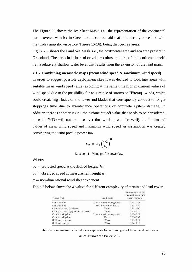
4.1.7. Combining mesoscale maps (mean wind speed & maximum wind speed) 39
4.1.8. Project Constraints 42
4.1.9. Sites Suggestions 44
4.2. Results PART II – Micro-scaling Analysis 46
4.2.1. Grid Independence – Results Site Suggestions 4,5 and 6 46
4.2.2. AEP determination 48
4.2.3 . AEP comparison 55
CHAPTER 5. DISCUSSION AND ANALYSIS 57
5.1. Part I 57

viii
viii
5.2. Part II 57
CHAPTER 6. CONCLUSIONS 61
6.1. Limitations and Future Work 63
REFERENCES 65
APPENDIX 1 - Script for data sorting (example meridional mean wind speed V) 69
APPENDIX 2 (Plotting – Example - UV) 70
APPENDIX 3 – Plotting (Geopotential example) 72
APPENDIX 4 – Vestas V90 3MW Power curve and technical specifications 73
APPENDIX 5 – Combination Maps Script (ffgmax example) 74
APPENDIX 6 – Multi-level data sorting (Site suggestion 4 example) 75
APPENDIX 7 – Multi-level data sorting excel table [partial] (Site suggestion. 4 at 70 m
example) 79
APPENDIX 8 – Wind profiles and mean wind speed variation per month (all site
suggestions) 80
APPENDIX 9 – California – Annual Average Wind speed at 80 m and Redding wind
farms location 82
siting
ix
ix
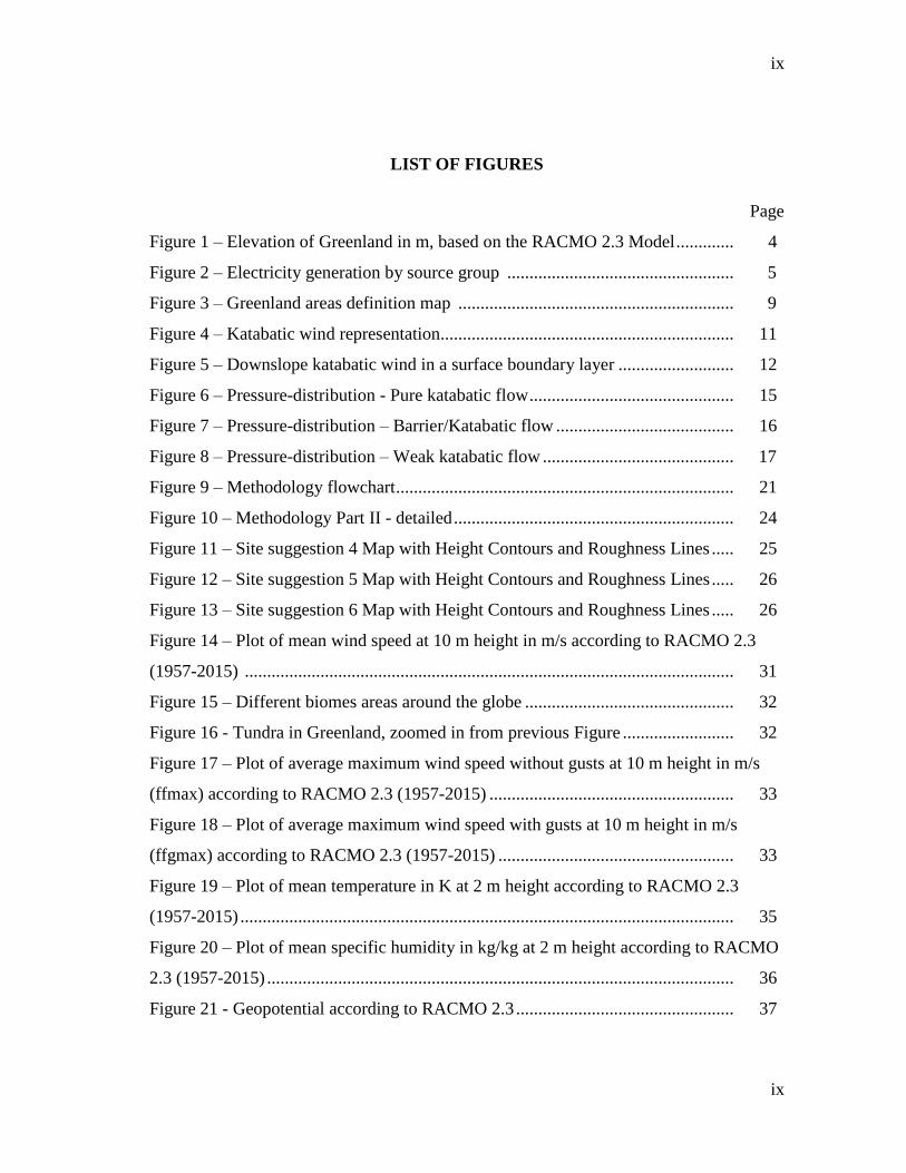
LIST OF FIGURES
Page
Figure 1 – Elevation of Greenland in m, based on the RACMO 2.3 Model ............. 4
Figure 2 – Electricity generation by source group ................................................... 5
Figure 3 – Greenland areas definition map .............................................................. 9
Figure 4 – Katabatic wind representation.................................................................. 11
Figure 5 – Downslope katabatic wind in a surface boundary layer .......................... 12
Figure 6 – Pressure-distribution - Pure katabatic flow .............................................. 15
Figure 7 – Pressure-distribution – Barrier/Katabatic flow ........................................ 16
Figure 8 – Pressure-distribution – Weak katabatic flow ........................................... 17
Figure 9 – Methodology flowchart ............................................................................ 21
Figure 10 – Methodology Part II - detailed ............................................................... 24
Figure 11 – Site suggestion 4 Map with Height Contours and Roughness Lines ..... 25
Figure 12 – Site suggestion 5 Map with Height Contours and Roughness Lines ..... 26
Figure 13 – Site suggestion 6 Map with Height Contours and Roughness Lines ..... 26
Figure 14 – Plot of mean wind speed at 10 m height in m/s according to RACMO 2.3
(1957-2015) .............................................................................................................. 31
Figure 15 – Different biomes areas around the globe ............................................... 32
Figure 16 - Tundra in Greenland, zoomed in from previous Figure ......................... 32
Figure 17 – Plot of average maximum wind speed without gusts at 10 m height in m/s
(ffmax) according to RACMO 2.3 (1957-2015) ....................................................... 33
Figure 18 – Plot of average maximum wind speed with gusts at 10 m height in m/s
(ffgmax) according to RACMO 2.3 (1957-2015) ..................................................... 33
Figure 19 – Plot of mean temperature in K at 2 m height according to RACMO 2.3
(1957-2015) ............................................................................................................... 35
Figure 20 – Plot of mean specific humidity in kg/kg at 2 m height according to RACMO
2.3 (1957-2015) ......................................................................................................... 36
Figure 21 - Geopotential according to RACMO 2.3 ................................................. 37

x
x
Figure 22 – Ice Sheet Mask according to RACMO 2.3 ............................................ 38
Figure 23 – Land Sea Mask according to RACMO 2.3 ............................................ 38
Figure 24 – Plots considering limitations regarding mean wind speed and maximum
wind speed ................................................................................................................. 41
Figure 25 - Preliminary site suggestions ................................................................... 42
Figure 26 – Mean wind speed at 10 m height with site suggestions (rough
approximation) .......................................................................................................... 44
Figure 27 – Final site suggestions ............................................................................. 46
Figure 28 –Mean Wind Speed [m/s] at 80 m site suggestions 4, 5 and 6 for full terrain
domain ..................................................................................................................... 46
Figure 29 – Convergence – Site suggestions 4, 5 and 6 ............................................ 47
Figure 30 – Wind Resource map at 80 m (Site suggestion 4) ................................... 49
Figure 31 – Site suggestion 4 – AEP results interpolated from each climatology height to
hub height .................................................................................................................. 50
Figure 32 – Wind Resource map at 80 m (Site suggestion 5) ................................... 51
Figure 33 – Site suggestion 5 - AEP results interpolated from each climatology height to
hub height .................................................................................................................. 52
Figure 34 – Wind Resource map at 80 m (Site suggestion 6) ................................... 53
Figure 35 – Site suggestion 6 - AEP results interpolated from each climatology height to
hub height .................................................................................................................. 54
Figure 36 – Interpolated AEP (80 m) results interpolated for all site suggestions
according to different climatology heights ................................................................ 55
Figure 37 – AEP results for all site suggestions with data from climatology at 70 m 56
Figure 38 – Vestas 3MW V90 power curve .............................................................. 73
Figure 39– Mean wind profile at climatology position – site suggestion 4 .............. 80
Figure 40– Mean wind profile at climatology position – site suggestion 5 .............. 80
Figure 41 – Mean wind profile at climatology position – site suggestion 6 ............. 80
Figure 42 – Mean wind speed site suggestion 4 - monthly variation ........................ 81
Figure 43 – Mean wind speed site suggestion 5 - monthly variation ........................ 81

xi
xi
Figure 44 – Mean wind speed site suggestion 6 - monthly variation ........................ 81
Figure 45 – California – Annual Average Wind speed at 80 m ................................ 82
Figure 46 – Wind Farms in the proximity of Redding (California) .......................... 82

xii
xii
LIST OF TABLES
Page
Table 1 Mean temperatures in selected towns in Greenland .................................. 10
Table 2 Non-dimensional wind shear exponents for various types of terrain and land
cover ................................................................................................................... 39
Table 3 Wind speed at hub height according to power law .................................... 40
Table 4 Preliminary site suggestions ...................................................................... 41
Table 5 Sites suggestions ....................................................................................... 44
Table 6 Site suggestion 4 - AEP results interpolated from each climatology height to
hub height .................................................................................................................. 50
Table 7 Site suggestion 5 - AEP results interpolated from each climatology height to
hub height .................................................................................................................. 52
Table 8 Site suggestion 6 - AEP results interpolated from each climatology height to
hub height .................................................................................................................. 54
Table 9 Vestas V90 3MW – Technical Specifications ........................................... 73
Table 10 Multi-level data sorting excel table [partial] (Site S.4 at 70 m example) . 79

1
CHAPTER 1. INTRODUCTION
Greenland is a vast land characterized by its extreme climate conditions and
extensive ice cap. Its energy production is extremely dependent on imported power
sources, although the potential for renewables such as wind, hydro or solar is
enormous. According to data obtained in 2015 (Greenland Statistics, 2015), the main
sources for energy production are fossil fuels, such as gas, oil, gasoline or kerosene,
resulting in a total of 555 ktons of CO2 emissions to the atmosphere. It should also be
noted that prospecting permits for oil exploration granted have increased every year
since 2008 (Statistics Greenland, 2015). Although finding oil locally could lead to a
decreased dependency on imported fossil fuels it would not impact the fact that
Greenland’s reliance on fossil fuels results in higher levels of CO2 emissions to the
atmosphere, which contributes to global warming.
Climate change is expected to have an enormous impact on Greenland’s landscape as
the increase in temperature will result in melting ice caps and could potentially
destroy the country’s unique ecosystem. Globally, the melting of the ice caps will
result in a sea level increase and would greatly impact a number of other countries.
Studies have shown that the surface mass balance (SMB) has been decreasing for the
last few decades (Lenaerts et al., 2012) as a result of global warming. Renewable
energy, and wind energy in particular, can play a major role as a viable solution not
only for the Greenlandic energy system but also for the preservation of the world’s
largest island.
In this project, the possibility for wind energy utilization in an artic climate was
investigated. To achieve this it is important to understand the wind phenomena in the
region as well as the wind speed distribution in the area.
Due to the constant severe climate conditions, it is difficult to perform physical
measurements in Greenland as instruments used to perform the tasks are sensitive to
these conditions. Therefore, for the purpose of this study, the data from a regional
atmospheric climate model, RACMO 2.3, improved specifically for polar climates by
the IMAU will be used.
Many studies have been performed using the RACMO model to accurately describe
weather conditions in Greenland; however the possibility for wind power utilization
in the artic climate has not been seen as a potential target before.
2
1.1. Justification of the research
Wind power development has grown exponentially in the last decade, and now
constitutes one of the most important renewable energy sources (GWEC, 2015).
Greenland is a vast area mainly covered by ice and has one of the most unique
ecosystems in the world. This environment is fragile, but is also rich in natural
resources. This combination unfortunately has led to a a high level of exploration for
fossil fuel sources.
Domestic energy consumption is traditionally based on oil and diesel generators,
which are highly polluting. These sources of production lead to an increase of CO2
emissions, endanger the ecosystem, and also accelerate the melting of the ice sheet
which in turn increases sea levels.
To prevent this situation from happening renewable sources of energy can be used
instead to meet Greenland’s energy needs. Unfortunately, Greenland has not yet been
well explored in terms of its wind power potential.
1.2. Scope of the research
The main goal of this thesis is to create a tool that can help potential wind developers
increase their interest in investing on the island. To assess the feasibility of wind
power in Greenland, its wind data must be analyzed.
Each site has its own challenges and Greenland, due to its unique conditions, is not
an exception. One of the challenges to be faced is the islands distinctive climate,
mainly characterized by low temperatures and specific winds. To better grasp the
nature of the challenge the climate characteristics are discussed in the literature
review section, with special focus on the wind.
The base data used for this research was provided by a Regional Atmospheric
Climate Model for a period of 58 years. The data consists of various characteristics
such as mean wind speed (eastward and meridional), maximum wind speed with and
without gusts, temperature, humidity as well as data regarding geopotential, ice and
the land-sea distribution.
Moreover, this data lead to the creation of a model and generation of mesoscale
maps. The analysis of these maps allowed for an assessment of potential for wind
power in the island. Data acquisition is not performed by the thesis’ author.
3
Furthermore, using the developed model as a tool to assess potential wind power
development sites, and setting important project constraints, three sites are chosen to
perform a microscale exercise. To achieve this goal, multi-level data was processed
by IMAU and a script was created to sort and organize the provided data.
The microscale analysis is done using primarily the WindSim software, but the
WindPro software was also used to assist in the creation of the terrain and
climatology files. The decision to use WindSim in the highly complex terrain
selected is explained in the literature review.
The results achieved are compared and a final site suggestion is made based on the
annual estimated production considering the coordinates of the three higher wind
resources within the terrain boundaries for each site.
Project limitations are discussed and future research suggested, as it was not possible
to perform a complete feasibility study due to time constraints.
1.3. Thesis outline
The thesis is divided into six main chapters. Chapter 2 consists on the description of
the location, the main energy sources and natural resources present on Greenland, as
well as the state of the art of renewable energy on the island. A comprehensive
description of the main weather characteristics with special focus on wind is also
performed. Furthermore a general description of the model from which the data was
obtained, and the justification behind the option for specific micro-scaling software is
explained. Chapter 3 explains the methodology and is subdivided into two parts. In
Chapter 4 the results from the methodology application are shown and compared
with results from similar studies (Part I). Discussion and analysis is provided in
Chapter 5. Chapter 6 presents the project conclusions, limitations and
recommendations for future work.
4
CHAPTER 2. LITERATURE REVIEW
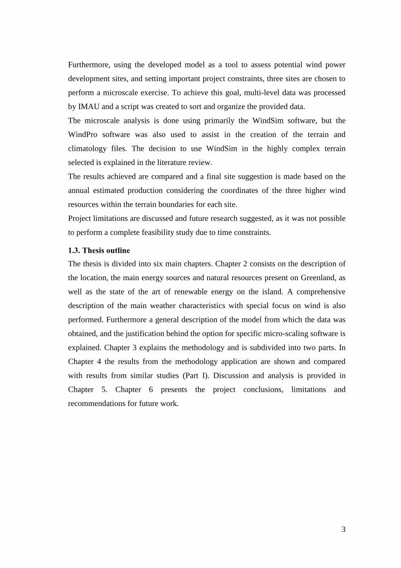
2.1. Greenland – General Data
Kalaallit Nunaat, also known as Greenland, is the largest island in the world. Located
between the Atlantic Ocean and the Arctic Ocean (geographical center coordinates
are approximately 72 00 North and 40 00 West), has a total area of 2.166.086 km2
and is mainly covered by the Greenland Ice Sheet (GrIS) or ice cap. The ice-free part
is roughly 20% of the island’s total area (Statistics Greenland, 2015).
The terrain elevation increases gradually from the coastline towards the center of the
island, (Figure 1) and the highest point is Gunnbjørn Fjeld (3693 m) (The Nordic
Council of Ministers,2016) can be found on the East of the island.
Figure 1 – Elevation of Greenland in m, based on RACMO 2.3
The terrain is generally characterized by an extensive ice sheet, which is flat with
gradual slopes, and with a sterile landscape of rocky mountains dominant on the
coastal regions.
The population of the island, according to Statistics Greenland (2015), was 55.984
habitants distributed among towns and small settlements with a population density of
0,028 /km2, or 0,14/ km2 in the ice-free areas, making it the least densely populated
region in the world.

5
The territory is part of the Kingdom of Denmark, but is self-governed since 2009.
2.2. Energy, natural resources and potential for renewables in Greenland
Nukissiorfiit is the only energy company in Greenland, dominating the market for the
supply and distribution of electricity, heating and water. As shown in Figure 2, where
the blue columns stand for oil products (gas oil being the main fossil product) and the
green for renewable energy sources (mainly hydro, but also biomass), the electricity
generation in Greenland has been taking huge steps towards sustainability since
2009. In 1999 almost 70 % of the electricity was provided by diesel generators (using
gas oil as a main source), but the situation has improved after 10 years, due to the
increase of hydropower on the island.
Figure 2 – Electricity generation by source group, Source: Baunbaek, L. (2014)
Nukissiorfiit is trying to help Greenland lead to its energy independency by
increasing the contribution of renewable energy to Greenland’s energy mix
(Baunbaek, 2014).
It is known that Greenland houses the biggest water mass in the Northern hemisphere
and the second in the world, just after Antarctica (Lenaerts, et al., 2012), and that it
can benefit tremendously by taking the path towards greener energy.
In September 2013, the Ilulissat hydroelectric plant started operating, and was the
first worldwide hydroelectric power plant to be constructed in a permafrost
environment. The energy produced by this hydroelectric plant itself is equivalent to
the consumption of 9 million liters of oil per year and will result in a yearly savings
of 20 kton of CO2 emissions (Landsvirkjun Power, 2016).

6
The company has some targets for the future which include the prioritization of
sustainable solutions as well as the reduction of CO2 emissions. As the expansion for
new or larger hydropower plants has been seen as a huge, unprofitable investment,
Nukissiorfiit instead started producing electricity using solar plants in 2014. The aim
of this project was to study the efficiency of solar energy on Greenland in order to
realize the potential of this renewable source on the future of the Greenlandic energy
system (Nukissiorfiit, 2013).
It is important to note that the information disclosed by the company has not included
wind power development as a possibility for the future. Despite this, the potential for
wind power will still be assessed.
Although Nukissirofitt is looking into sustainability, it is also important to note that
Greenland is one of the wealthiest countries in the world in terms of natural resources
including an enormous amount of minerals such as the so called “rare earth metals”
as well as, “iron ore, gold, zinc rubies, gemstones and uranium” (Wilson, 2015). It is
even stated, that just the “Kvanefjeld” deposit itself, contains around 260,000 tons of
uranium, and that the difficulty in modifying Greenlandic and Danish policies (since
defense and security policies are Denmark’s responsibility) to facilitate exportation
and control of this mineral, can result in the uranium be used as “nuclear fuel” to
produce electricity on Greenland.
Smits, et al.(2016), released a report predicting that the waters around the island hold
large amounts of unexplored oil and gas, which is reinforced by statistics showing
that the number of exploration permits granted had doubled from 2008 to 2013
(Statistics Greenland, 2015). All of this could allow Greenland to become energy
independent, but could also subsequently lead to an overall loss of interest in
renewable energy systems.
2.2.1. State of the Art of Renewables in Greenland
As it was mentioned earlier, Nukissirofitt is aiming to increase the share of
renewables in Greenland’s energy mix. For the moment hydro and solar have been
studied as potential candidates, nevertheless, both sources of energy possess some
particularities that are important to take into consideration, and that can reinforce the
importance of wind power feasibility studies.

7
2.2.1.1. The specific case of hydropower and the aluminum smelting industry
Although some setbacks regarding the way to a sustainable Greenland were
discussed before, the “symbiotic connection” between hydro and aluminum smelting
has been gaining some strength. The aluminum smelting industry is highly energy
dependent which together with the huge potential for natural refrigeration, provided
by Greenland’s artic climate, can lead to an expansion of hydropower. In 2006,
Alcoa, an American company studied the potential of installing an aluminum smelter
unit in Maniitsoq, Greenland (Wilson, 2015).
The project had the intention of using water tanks as an extension of the regional
lakes and drilling to create a piping system that would allow the water in the tanks to
flow to underground powerhouses, feeding the hydro reservoirs from the glacier melt
in the summer and then lowering during the winter in order to have enough water for
the power generation (Bjarnoson, 2007). Even though the project was seen as
economically beneficial both for the local government and Alcoa, the partnership
encountered a few hurdles, mainly in the form social acceptance issues and
environmental risks. This resulted in the project being placed on the “waiting list” for
resolution. If approved, this project can open the door for other companies to transfer
their facilities to Greenland, leading to an overall growth of global renewable energy
(Wilson, 2015).
2.2.1.2 Solar Energy
Dragsted (2011) assessed the potential of using solar energy for heating purposes in
Sisimiut, Greenland. She verified that the positioning of the sun, due to the high
latitude values of the island, is very different compared to many places in the world.
This high latitude values influence the sun position, it is lower in the sky, and results
in a higher tilt angle of the receptor, leading to an increase in efficiency of solar
energy. This coupled with the ”white nights” Greenland experiences during the
summer (24 hours daylight) and the reflectivity from the snow tilted towards
receptors results in both high and efficient power production during the summer. The
amount of energy produce was able to provide households with enough hot water as
well as enough for hot water for heating systems. However, during the winter time, it

8
was verified that the system does not work, mainly due to the near absence of sun-
light (Dragsted, 2011).
Solar energy can actually became one of the main energy resources in Greenland, but
proper storage systems are needed to allow the population from the island save the
excess energy generated during summer for usage during the winter time.
Unfortunately, energy storage devices are currently not advanced enough to support
this kind of solution.
2.2.1.3 Wind Power
The growth of hydropower presented in Section 2.2.1.1 shows an increasing trend.
However hydro will be mainly dedicated to supplying power for industrial uses.
On the other hand, the study regarding solar power shows that the potential, however
high during the summer, is non-existent during the winter. Thus, unless the energy
storage industry finds a solution in a near future, the energy extraction from the sun
will remain on hold for the island.
Due to these factors, the domestic consumption on Greenland will continue to be
provided by traditional oil or diesel generators. This means Greenland will remain
dependent on external sources of energy and its CO2 emission levels will not
continue decreasing. Therefore, wind power, if effective, could be a solution for the
issue. According to Greenland Statistics (2015), wind power is not present in the
energy mix of Greenland.
2.3. Weather Characteristics
2.3.1. General overview
Greenland is characterized by having an arctic climate (Lyck and Taagholt, 1986),
this means that the highest temperatures during the summer do not exceed 10 °C.
More accurately, Greenland can be is divided into different climate areas, as it can be
seen in Figure 3:

9
Figure 3 – Greenland areas definition map, Source: van Angelen et.al, 2011
In the southwest (SW) region the temperature variations are in fact quite similar to
the ones seen in Denmark, however with different absolute values. The precipitation
is higher when compared to Danish statistics, and takes place on a more regular
basis. The southwest region is affected by gusts year around and freezing fog occurs
often (Lyck and Taagholt, 1986).
The west coast (W), characterized by a large number of “fjords”, presents a similar
climate to the one recorded in continental areas, with gusts often recorded during the
winter (Lyck and Taagholt, 1986). This is a result of the predominant katabatic flow
in the region. Katabatic flow refers to winds that arise when cold air with high
density is forced down a slope by the gravitational force and consequently increasing
its speed (Stull, 2009), this is explained with more detail in Section 2.3.2.1.
In the northern region, the temperature variations are higher than in the other zones.
Mean temperatures and wind speeds are particularly low, gusts are rare and
precipitation levels are almost insignificant, for these reasons, some of the northern
areas are named “arctic deserts” (Lyck and Taagholt, 1986).
The eastern region (E) presents lower temperatures during the summer when
compared to the Western area (Lyck and Taagholt, 1986). This can be explained by
the “drifting polar ice” phenomena, which are ice floes (a sheet of floating ice) that
are created by the instability of the top surface of the ice layers. This instability can
be created by “solar, atmospheric, oceanic and tidal forcing” (Lepparanta, 2005).
Precipitation is common in this area, and winds are unstable, varying suddenly with
gusts all over the “fjords”. The following table shows the mean temperature for the

10
different months of 2014. The abbreviations next to the name of the selected towns
represent the geographical region that they are located in:
Nonortalik (SW)
Nukk (W)
Kangerlussuaq (W)
Ilulissat (W)
Tassilaq (E)
Table 1 – Mean temperatures in selected towns in Greenland, Source: Statistics Greenland,
2015
Greenland is an enormous land mass with different climate characteristics and the
climate variations are notorious from region to region. However, as the main purpose
of this project is focused on the feasibility of wind power, the wind’s characteristics
will be discussed in greater detail than other weather characteristics.
2.3.2. Greenlandic Winds
The winds over Greenland differ from the ones seen in Continental Europe. They are
quite local in nature, in large part due to the low temperature conditions, high level of
temperature variations between the tundra and the GrIS as well as the island’s
orographic complexity (mainly at the coastline). A short description of the different
wind phenomenon experienced on Greenland is given below.

11
2.3.2.1. Katabatic Winds
Greenland can be seen as a massive mountain of solid ice. When stable air over the
center of the ice sheet, with relatively high pressure, maintains its placement for a
long period of time it will cool down due to heat transfer with the ambient
temperature. By getting cooler the air increases its density, forcing it down the high
Greenlandic slopes (van den Broeke, M.R. et al., 1993). Figure 4 represents the
katabatic winds.
Figure 4 – Katabatic wind representation, Source: Grobe, et al., 2007
The opposite can also happen, the air is heated up by the ice sheet, when the ambient
temperature is lower than the ice sheet, resulting in air being “pushed” up to the
slopes.
Katabatic winds can be physically explained by analyzing the momentum balance
equation, and assuming that the flow is hydrostatic, shallow and two dimensional
(δ/δy)=0, according to (Mahrt 1982):
𝛿𝑢
𝛿𝑡+ 𝑢
𝛿𝑢
𝛿𝑥+ 𝑤
𝛿𝑢
𝛿𝑧= 𝑔
𝜃𝑑
𝜃0sin α + cos 𝛼
𝑔
𝜃0
𝜕(𝜃𝑑ℎ)
𝛿𝑥+ 𝑓𝑣 −
𝛿𝑢′𝑤′
𝛿𝑧
1 2 3 4 5 6 7
Equation 1: momentum balance equation

12
Where:
x, y and z = 3 dimensions in an infinitesimal cubic element
u = velocity along the slope
v = lateral velocity to the slope
w = velocity perpendicular to the slope
α = slope angle
θd = temperature difference of the layer compared to the background
θ0 = background temperature
h = layer thickness
g = acceleration of gravity
f = Coriolis force parameter
And where each of equation 1 terms represent:
1 – Acceleration
2 – Downslope advection
3 – Vertical advection
4 – Buoyancy
5 – Thermal wind
6 – Coriolis effect
7 – Stress divergence
(Stull, 2009)
The physics behind the katabatic flow are described by the first term on the right
hand side of equation 1 (term 4); therefore it can be seen that it depends on the
acceleration of gravity (g), the temperature variation coefficient θd/θ0 and the
inclination of the slope given by sin α. Depending on the weather setup on the coast
this effect can be prevented or enhanced, i.e., making the flow stronger or weaker.
For a better interpretation of equation 1 a representation of the downslope katabatic
winds as well as the coordinate system used in is shown in Figure 5:

13
Figure 5 – Downslope katabatic wind in a surface boundary layer,
Source: Stull, 2009
In order to further clarify this, it is rather common to have a low pressure system on
the southeast of the island opposed to a high pressure system on the southwest.
Moreover due to the geographic local of Greenland (the Northern Hemisphere), the
Coriolis effect states that low pressure systems rotate counterclockwise and high
pressure systems clockwise. If a cool parcel of air is placed in the center of the GrIS,
it will follow the low pressure system, creating a channeling effect and consequently,
high wind speeds. This flow is dry resulting in a lack of humidity in the center of the
GrIS and dominant katabatic winds all year. It is also important to note that as the
flow approaches the limits of the ice sheet it gets weaker and lower wind speeds are
observed at the edge of the GrIS (Ettema et al., 2010,b). The katabatic winds are
created by the intense energy transfer between ice and air, but they are also
dependent on the conditions of the terrain, and while they are observed in many other
parts of the globe, they are common both in Greenland as well as in Antarctica
(Mathiot et al., 2010).
Studies also show that the katabatic flow is relatively stronger during the winter than
during the summer, which is caused by the temperature fluctuations between these
two different seasons (Ettema et al, 2010,a).
It is, however, important to note in closing that the phenomena of katabatic winds
over Greenland has not been analyzed with any frequency or for long periods (van
den Broeke et al., 1993).

14
2.3.2.2. Barrier Winds
These jets are formed due to the interaction between the ice sheet and the tundra (by
the coast, which presents higher temperature values). Barrier winds are normally
observed in the “melting zone” where the temperature variation is more abrupt and
the interaction with katabatic winds is rather common. As they are thermal winds
they can transport warm air, and are extremely important in the development of
studies regarding the melting of the ice cap (van den Broeke et al., 1996). As
discussed by van den Broeke, et al. (1996), during a study on the western part of
Greenland, and event is described by being a pure interaction between the air
generated by the warm and cold surfaces. Even though the event was observed
during the summer season, it could not be determined if it occurs frequently.
On the other hand studies performed in the southeast of the island by Harden and
Renfrew (2011) with a larger sample (20 years), contradicted van den Broeke et al.
(1996). Harden and Renfrew (2011) found that these winds were not formed
exclusively due to the temperature exchange between the tundra and the ice cap, but
that the event was provoked by the topographic complexity (height contours) in the
coastal areas. This seems to be confirmed by the studies conducted by Moore and
Renfrew (2005) which stated that especially by the coast, Greenland presents a
moderate to high orographic complexity that leads to the formation of relatively high
wind speeds named “barrier winds”. Important to mention that Harden and Renfrew
(2011) state that this phenomena had been observed in many different places such as
Antarctica, Alaska, California or New Zealand, and always at high altitudes. This
reinforces that barrier winds are also highly influenced by terrain complexity.
2.3.2.3. “Piteraq” Winds
As was noted in Section 2.3.2.1, katabatic flow is largely present over Greenland’s
surface, being more frequent during the cold seasons (Autumn and Winter). During
these seasons, the flow is stronger, with very high wind speeds, induced by the
extremely low values of surface net radiation (i.e., the balance between the absorbed
energy and released energy from the sun at the top of the atmospheric layer). When
aligned with the large-scale geostrophic wind (van As et al., 2014), “Piteraq” winds
can occur (Earthobservatory.nasa.gov., 2016). Piteraq winds means “the one that

15
attacks” in the local language and they are described as a “hurricane-like” wind
(Cappelen et al., 2001).
For example, the third highest wind speed ever recorded in the world was registered
in 1972 in the town of Thule in NW Greenland, with wind speeds around 93 m/s.
Recently (2013), this type of event endangered the life of the participants on an ice
cap expedition, with a registered wind speed of 42 m/s. Due to the main
characteristic of high wind speed, Piteraq winds can have a major influence on the
ice cap and its borders with the tundra (van As et al., 2014).
2.3.3. Typical flows over Greenland
During the summers of 1990 and 1991 an experiment (Greenland Margin Experiment
– GIMEX-90/91) was conducted by Van der Brooke et al. (1996) near Søndre
Strømfjord, in the west (W) part of the island which, among other conclusions, led to
a classification of different flow types over Greenland.
2.3.3.1. Pure Katabatic
In a pure katabatic flow, high pressure systems are predominant over the north and
center of the island, covering a large area corresponding to the ice cap. It can be
observed in Figure 6 that on the southern area (both on the east and west side) a low
pressure system is predominant. This is described as being the typical pressure-
distribution over the Greenlandic Island.
The tundra is relatively warm, especially during the summer, but cold air coming
from the interior of the ice cap does not allow the temperature to increase in the
border area between the GrIS and the tundra. In this area the flow is “purely
katabatic”, not being affected by the large-scale circulation winds (van den Broeke et
al., 1996).
Figure 6 – Pressure-distribution - Pure katabatic flow – Source: van den Broeke et al., 1996

16
2.3.3.2. Barrier/Katabatic
By analyzing Figures 6 and 7, it can be stated that the high pressure system moved
from the ice cap area towards the northeast region, allowing the low pressure system
situated on the southeast region in Figure 3 to approach the western region. This low
pressure system moves the air from the tundra (warmer air), via advection, in the
direction of the ice sheet. This temperature variation will lead the creation of thermal
conducted winds, which were described before as barrier winds.
The already katabatic flow enhanced with this thermal conducted barrier winds will
cause a strong surface-wind speed in the margins of the GrIS.
Figure 7 – Pressure-distribution – Barrier/Katabatic flow – Source: van den Broeke, et al, 1996
2.3.3.3. Weak Katabatic
This case shows the predominance of low pressure systems in the east side of the
island. Cold air advected from this low pressure system situated on the northern areas
of Greenland (Figure 8), will cool the areas over the tundra. Therefore, the
temperature variation will be smaller (close to 0 °C). Barrier winds will not exist in
this case, as the effect of thermally conducted winds will be almost inexistent. If the
temperature of the surface air does not change to values below 0 °C, the weak
katabatic flow will be predominant on the border between tundra and ice cap.

17
Figure 8 – Pressure-distribution – Weak katabatic flow – Source: van den Broeke, et al., 1996
2.4. Mesoscale Models
Mesoscale models will help the developer assess, at the preliminary phase, which are
the potential sites for wind power development. This rough approach is not based on
on-site measurements, but provides an approximation of the reality. It is normally
based on data from satellites, long term data reanalysis, and also meteorological
modelling (ESMAP, 2010). The data for the present study was provided by a regional
atmospheric model – the RACMO 2.3 model.
2.4.1. The RACMO 2.3 model
The Regional Atmospheric Climate Model or RACMO2.3 (hereafter RACMO2), was
created by the Royal Netherlands Meteorological Institute (KNMI) (Van Meijaard et
al., 2008), which is still responsible for the management and improvement of the
model.
RACMO2 results from the interaction between two numerical models, using the
atmospheric physics processes behind the European Centre for Medium Range
Weather Forecast – Integrated Forecast System (ECMWF-IF cycle CY33rl, van
Wessem et al., 2014) and the atmospheric dynamics derived from the “High
Resolution Limited Area Model (HIRLAM) (Undén et al., 2002).
A dedicated version for polar climate was elaborated by the IMAU, in order to get a
specific representation of the surface mass balance of the Greenlandic and Antarctic
ice caps, as well as other glacial areas (Noël et al., 2014).
The model’s domain has a horizontal resolution of ≈11 km and a vertical resolution
of 40 atmospheric hybrid-levels (Ettema et al., 2010a). It possesses 306 × 312 grid
18
points, which include Greenland, Arctic Canada, the Svalbard Islands and Iceland
(Gorter et al., 2013).
The system is forced on the lateral boundaries on a 6 hour interval by the re-analyses
from ERA-40 (1958-1978) and ERA-INTERIM (1979-2015) (Noël et al., 2015).
RACMO2 represents the katabatic regime over Greenland realistically; however the
model’s grid is 11 km which does not present solutions for small scale circulations
(van Angelen, et al., 2011).
2.4.2. Main studies using RACMO
The model had been already used in a number of different studies, such as:
- Climate of the Greenland Ice Sheet using a high resolution model – part 1:
Evaluation/part 2: near surface climate and energy balance – J. Ettema et al.,
2010.
- Momentum budget of the atmospheric boundary layer over the Greenland Ice
Sheet and its surroundings – J.H. van Angelen et al., 2011)
- Drifting snow climate of the Greenland Ice Sheet: A study with a regional
climate model – J.T.M. Lenaerts et al., 2012)
- Present and future near surface wind climate of Greenland from high
resolution regional modelling – W.Gorter et al., 2013
- Impact of summer snowfall events on GrIS SMB – B. Noël et al., 2014
2.5. Micro-scaling
In order to perform a micro-scaling analysis, a specific wind engineering model is
crucial. Many factors can affect the energy yield of a wind farm. And a badly
performed estimation can result in high revenue losses for the developer. There
currently exist a few available to help solve these problems. WindSim, WindPro and
WaSP are some of the more commonly used commercially available tools.
2.5.1. WindPro
WindPro is a wind farm design tool used to both plan and design solutions for wind
farms. The software was designed based on 25 years of experience in wind power
project development. The software is comprised of a large number of modules which
allow the developer to assess information for the specific purposes related to their

19
wind farm development. The modules are largely independent of each other, which
makes the program more accessible (EMD, n.d.).
Besides being able to calculate the energy yield from a wind farm, the program is
also able to calculate noise and flicker for the households in the vicinity of the
windfarm, to create photomontages and animations, verify losses due to electrical
connections and many other features. It is especially accurate in map digitalization,
namely height contours and is connected to large map databases. For the purpose of
this study, WindPro was used as an auxiliary tool for map creation (see Section
3.2.1), and for generation of frequency tables that were transformed into climatology
files (see Section 3.2.5.3).
2.5.2. WaSP
Wasp is a linear model wind simulation tool developed by the Risø National
Laboratories in conjunction with the Technical University of Denmark (DTU). WaSP
allows the developer to find the best site locations for wind turbine construction
based on the wind conditions and energy yield.
WaSP is considered to be a good tool to optimize the production of a wind farm and
perform wind resource assessment even in terrains with moderate orographic
complexity (WaSP, n.d.).
However, studies, such as the ones perform by Nilsson (2010) or Zhang (2015), have
shown that WaSP is not accurate enough when flow separation occurs, i.e., if a slope
is higher than 17°, as the speed-up effect is not linear. And as the program does not
consider accurately high slopes (inclinations >17°) this can lead to an overestimation
of the energy production.
2.5.3. WindSim
WindSim is wind simulation software that allows the developer to optimize the
energy yield from a wind farm without compromising turbine load limits. The
software uses CFD (computational fluid dynamics), meaning it was developed to find
solutions for various fluid flow equations (WindSim, n.d.). By analyzing the data
provided for different wind speeds and directions, the model can accurately find the
best positions for turbine erection in a pre-determined area. This data can be provided
by measurements, but data provided by meteorological models are also acceptable.
20
To calculate the wind distribution and its characteristics, WindSim correlates the
terrain and atmosphere as a whole in three-dimensions while solving the Navier-
Stokes equation in an iterative way for every grid point. The Navier-Stokes equations
can help to describe the behavior of a fluid flow, which are known to be of difficult
resolution and unstable.
To solve micro-siting problems, the program should be run in its six modules:
Terrain, WindFields, Objects, Results, Wind Resources and Energy (Meissner 2010).
Even though the software is especially accurate in sites of high orographic
complexity, it does not permit the digitalization of maps; therefore another program
such as WindPro, for instance, is necessary (Nilsson, 2010).
2.5.4. Model Selection
To understand which would be the best suited software for the thesis an important
feature should be questioned: which is the software that will provide the best results
in terrain with higher complexity? Nilsson (2010) found that by simulating data and
comparing the results from two different softwares (WaSP and WindSim) that WaSP
(a linear model) is in fact more efficient than WindSim (a non-linear model) when
the terrain complexity is low, leading to lower computational time, however, as the
complexity of the terrain increases WaSP becomes less accurate as it does not take
into account the turbulence effects that occur in sites with complex orography. As the
terrain complexity on the coast of Greenland is high, characterized by steep, rocky
mountains (see section 2.1), WindSim appears to be the best suited for this study.
21
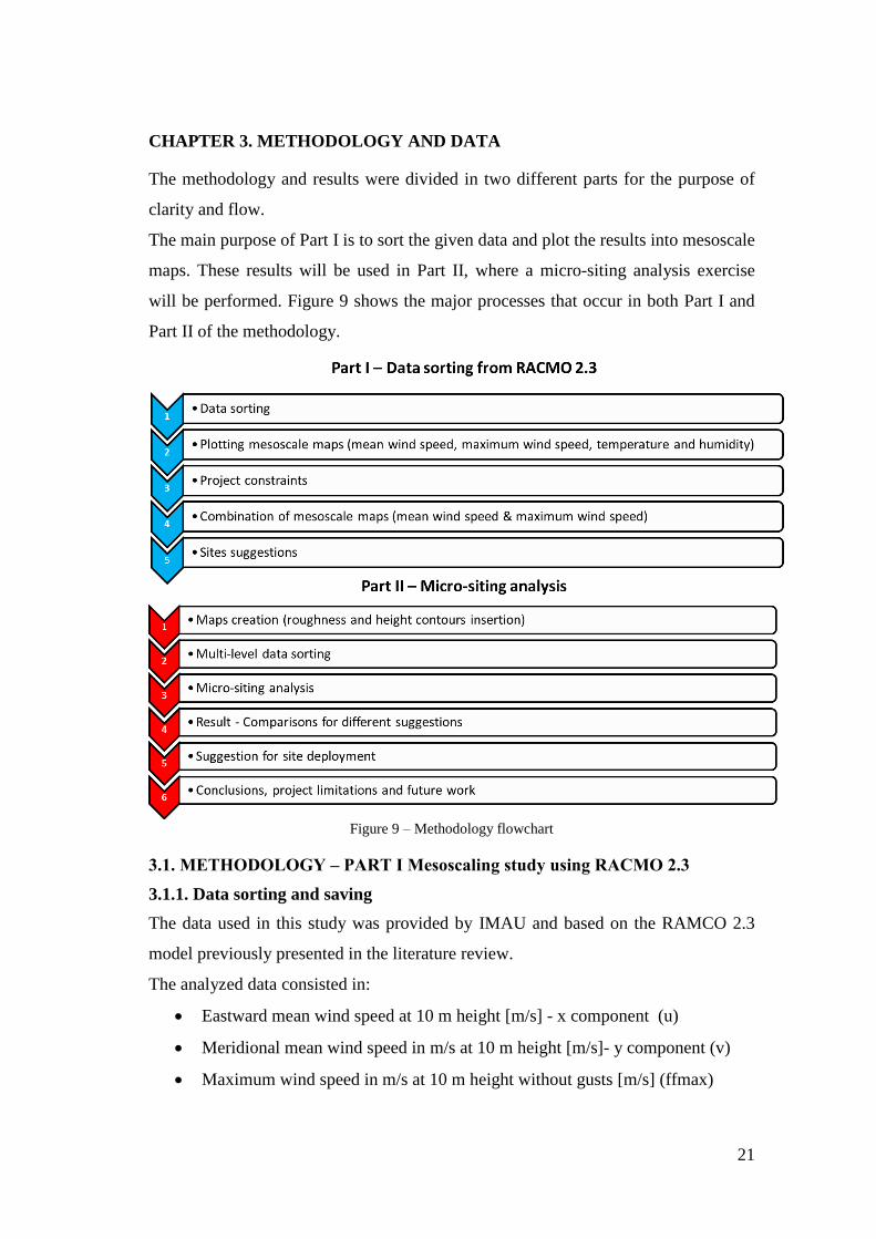
CHAPTER 3. METHODOLOGY AND DATA
The methodology and results were divided in two different parts for the purpose of
clarity and flow.
The main purpose of Part I is to sort the given data and plot the results into mesoscale
maps. These results will be used in Part II, where a micro-siting analysis exercise
will be performed. Figure 9 shows the major processes that occur in both Part I and
Part II of the methodology.
Figure 9 – Methodology flowchart
3.1. METHODOLOGY – PART I Mesoscaling study using RACMO 2.3
3.1.1. Data sorting and saving
The data used in this study was provided by IMAU and based on the RAMCO 2.3
model previously presented in the literature review.
The analyzed data consisted in:
Eastward mean wind speed at 10 m height [m/s] - x component (u)
Meridional mean wind speed in m/s at 10 m height [m/s]- y component (v)
Maximum wind speed in m/s at 10 m height without gusts [m/s] (ffmax)

22
Maximum wind speed in m/s at 10 m height with gusts [m/s] (ffgmax)
Temperature at 2 m height [K] (T)
Specific humidity at 2 m height [kg/kg] (q)
Geopotential, Land Sea Mask, Ice Sheet Mask
The data was provided in the form of netcdf files, or “network common data form
which can be described as a set of interfaces for array-oriented data access”. They
provide a way to share large databases of information in compressed format and
enable the files to be used without changing its structure. (Unidata, n.d.).
For example, the information for the eastward mean wind speed (u), extracted from
the netcdf file for data sorting were: latitude, longitude, time, height and eastward
mean wind speed variables. Each one of these variables comprises different
dimensions, attributes and the size, which can vary from a 2D array to a 4D array.
Matlab was selected as the tool to use to access the netcdf files. Although Matlab
does not possess an internal netcdf library, a specific toolbox (mexcdf.r4053) was
found online and was available to download. This toolbox allows Matlab to process
the netcdf files. The data was sorted and saved in a mat file, allowing for subsequent
data processing of the information. The script for data sorting can be found in
Appendix 1.
3.1.2. Plotting Mesoscale maps explanation
With all the data saved into mat files, a way to visualize the data was necessary. To
perform this “picturing” a path to create a map with all the combined information
was desirable. As Matlab does not possess an internal map library a toolbox
(m_maps) was found online and downloaded.
All the variables were combined by date decade (with exception of the first file). For
example, the mean wind speed at 10 m height, for the period 1961-1971 was
compiled considering all grid points (latitude and longitude).
The two wind components were combined using the following vector equation:
𝑈𝑉 = √𝑢2 + 𝑣2
Equation 2 – Vector composition of mean wind flow

23
However, the resultant 4D arrays (latitude, longitude, height and mean wind speed)
were too heavy for computation, as Matlab does not allow 4D arrays with dimensions
greater than 10,000 elements (21,306 were needed) ,therefore another solution had to
be found.
As the “height” variable was considered unnecessary, i.e, it is constant; the plot of
the mean values in relation to the time variable was executed, resulting in a lower
computational time (“lighter file”). This 2D array was then plotted for the different
variables, cited in Section 3.1.1. (The script regarding u and v combined can be
found in Appendix 2 as an example). The scripts for ffmax, ffgmax, T and q are
similar with exception for the variable names, therefore are not shown in an
appendix. The Geopotential, Ice Sheet Mask and Land Sea Mask were also plotted
(the script for the Geopotential can be found in Appendix 3). The scripts for Ice
Sheet Mask, Land Sea Mask are similar with exception for the variable names,
therefore are not shown in an appendix. The definition of each one of these variables
as well as the resultant maps for all variables are shown in chapter 4.
3.1.3. Project constraints
Greenland is a unique environment. Some of the distinct characteristics that make the
island so special were analyzed leading to the development of the constraints. As
they directly affect the final site suggestions, their description has been placed in the
results section (4.1.8).
3.1.4. Combination of mesoscale maps
Having the results from the wind speeds (at 10 m height) and the project constraints
defined it is possible to select potential sites for wind power development and request
multi-level data (at different heights).
The combination performed will take into account the areas with mean wind speed
considered as suitable for wind power development and avoid areas where the
averaged maximum wind speed, including gusts, are seen as potentially hazardous to
the wind turbine. More detailed information can be seen in Section 4.1.7.

24
3.2. METHODOLOGY – PART II – Micro-siting analysis
Based on the results from part I, the data was organized and the micro-siting analysis
exercise was performed for three suggested sites.
A detailed flowchart is presented to map the process in Figure 10:
Figure 10 – Methodology Part II - detailed
The following sections describe the methodology used for Part II.
3.2.1. Map Insertion
The resulting coordinates from the three different sites, from the results of Part I (site
suggestions 4, 5 and 6, see section 4.1.9) were input into the software WindPRo in
order to search for the chosen sites.
The maps were selected from online data, provided by the software, based in the
satellite images from the US GeoCover database.
The map specifications were provided manually, and a width of 20.000 m and height
of 20.000 m was selected.
After this process the maps for each site were generated.
3.2.1.1. Roughness Insertion
Roughness length refers to the height where the wind speed is theoretically equal to
zero. Increased roughness length can lead to higher turbulence, which consequently
affects the wind (Stull, 2009).

25
For each generated map, roughness details were inserted. The roughness data was
selected from online data, provided by WindPro, based on the “Global cover 2009
Dataset”. At last, the width and height were defined as 20.000 m by 20.000 m.
3.2.1.2. Height Contours Insertion
Height contours also called elevation can affect largely the wind data. For example
(Brower and Baley, 2012) stated that wind data is more representative when the
terrain elevation is constant. On the contrary he also refers that the complexity of the
terrain can affect wind data reliability.
For each generated map, height contours data was also inserted. This data was
selected from online data provided by WindPro and based on the “View Finder
Panoramas” database.
The width and height were set as 20.000 m by 20.000m.
The final maps of suggested sites 4, 5 and 6 with roughness (on the left side) and
height contours (on the right side) can be seen in Figure 11, 12 and 13 respectively:
Figure 11 – Map of site 4 with Height Contours and Roughness Lines - Source: WindPro (2016)

26
Figure 12 – Map of site 5 with Height Contours and Roughness Lines – Source: WindPro (2016)
Figure 13 – Map of site 6 with Height Contours and Roughness Lines– Source: WindPro (2016)
3.2.2. Map File Creation
After processing all data in WindPro, another sub-process needed to be performed.
The process is common to all the suggested sites and involves the creation of a map
file. The purpose is to combine all the compiled information for the different sites
suggestions (map, roughness and height contours) into a single map file for further
inputting in WindSim.
3.2.3. Multi-level data sorting
As the wind speed data provided by IMAU, was modelled only for 10 m height, new
data was required to perform the micro-scaling analysis exercise.

27
This data was processed for different levels and provided for 10, 35, 70, 100 and 120
m, for the three chosen locations.
Important to refer that RACMO has a ≈ 11 km grid in the horizontal axis, therefore
the climatology data provided was sorted to the closest grid point of the suggested
site centers for site 4, 5 and 6.
3.2.3.1. Script description
In order to extract the information from the files containing the multi-level data for
the three suggested sites presented, a new script was written in Matlab (see appendix
6). The output of this script consisted of two different kind of files, a txt file for
subsequent conversion in WindSim and an xlsx file for data confirmation.
The multi-level data extracted from the new netcdf files had information relative to
the two wind components, x component (u) and y component (v) as well as
information regarding their wind direction and respective time stamp (year, month
,day and hour) for each level (10m, 35m, 70m, 100m and 120 m). The resultant wind
speed was therefore calculated on the script using the same principle shown in
equation 2. A partial example of the table created with the script is shown in
Appendix 7.
3.2.4. Generation of time series file (tab file)
To create a climatology file in WindSim, the creation of a tab file (WaSP file) is
needed for later conversion.
For that reason the file created with the script described in section 3.2.3.1, was
inputted in WindPro as a frequency table for each level. When exported this
information generates a tab file.
Having created these files of given frequency distributions and time stamps to the
different heights (10m, 35m, 70m, 100m and 120m), it is possible to convert it into a
climatology file in WindSim (wws file see section 3.2.5.3).
3.2.5. Micro siting analysis (WindSim)
3.2.5.1. Terrain
This module generates a 3D model of the selected area based on its elevation (height
contours) and roughness data. It is possible to modulate different types of modules
objects in terrain that can influence the flow (WindSim, n.d.).
28
Using the map file created according to the process described in the section 3.2.2, a
gws file can be derived for WindSim, so the software is able to read it as a terrain file
(gws). This allows the terrain to be created based on the roughness and height
countors data from the map file.
The method used to convert this file is simple: after opening WindSim, the menu
“Tools” should be chosen and the option “Convert terrain model” selected. This
opens a window where the map file can be selected and converted to a gws file.
3.2.5.2. WindFields
The “WindFields” module processes the generated “Terrain” by simulating the
windfiels through the Reynolds Averaged Navier-Stokes equation (RANS). For this
calculation the “Standard k-epsilon” turbulence model was used. As the RANS
equation is non-linear the simulation solves the equation iteratively until covergence
(Meissner, 2010).
In the case of the simulations performed for this project, the number of iterations was
defined as 100 primarily, however all suggested sites were not showing convergence
and the number of iterations was increased to 500. For all sectors (12 sectors between
30°- 360° with 30° increments in a wind rose), all sites converged before 350
iterations. The potential temperature was disregarded and the air density used was
1.225 kg/m3 (as default). The boundary layer level was increased to 1000 m and the
wind speed above the boundary layer was set as 10 m/s (as default). For ”number of
cells in z direction” 30 nodes were considered, allowing to refine the terrain above
the turbines hub height. This is made in order to achieve higher definition at the
lower levels.
3.2.5.3. Objects
This software feature allows the insertion of data relative to climatology as well as
turbines positions in order to simulate data in different positions of the terrain. The
“Terrain Model” and “WindFields” modules have to be already run to be able to
start the object module. To add turbines or climatology data the tab “Park Layout”
should be chosen. Subsequently, there is the need to select the icon depending on the
inputted object and choose its characteristics.
Although WindSim possesses a database for turbines, this is relatively small.
However the power curve data can be edited, modified or added in the form of a pws

29
file. For the purpose of this study, 3 turbines, Vestas V90 3MW with a hub height of
80m were chosen as an example, as the choice of turbine is not within the scope of
the thesis.
To generate the climatology files it is necessary to convert the data in the tab (WAsP
file) to WindSim. The data from the tab file is converted using WindSim toolbar and
the climatology file wws is generated.
3.2.5.4. Wind Resources
This module allows the visualization of the wind resource maps for different
climatology and allows the extraction of information concerning wind resource
distribution inside a pre-defined terrain. This can be done for several heights.
For the project in study wakes were disregarded.
The information provided by this model contains characteristics such as the wind
speed and power density maps, as well as, the wind rose and the Weibull distribuition
graph where the K and Γ parameters are presented in form of a table.
3.2.5.5. Energy
According to the objects inserted before, the AEP is calculated. For each climatology
data is inputted. After running, the module displays data considering both frequency
table and Weibull distribution. Wake effectes can be considered and the height of
reference production should be set. In the thesis, this was set as 80 m. For each
climatology, AEP data regarding each turbine can be also obtained. Information such
as mean wind speed, power density, full load hours as well as gross AEP are
displayed.
3.2.5.6. Grid Independency
The grid in study for each site suggestion should be independent. This means that, it
is important to find when the domain becomes stable, or in other words, discover the
amount of cells that the grid should consist of in order to have a behaviour
resembling the reality without depending of changeable input parameters.
As the study had no guidance regarding turbines position, instead of running the
energy model and compare the AEP results for a crescent number of cells (common
method used), another path was taken. This choice can be justified by the large
domain size (20000 m × 20000 m) but also by the fact that inputing a turbine in any

30
position within the terrain would provide the independency of one singular grid
point.
The applied method is described as follow:
Firstly the terrain and windfields modules are run considering 500.000 as minimum
number of cells increasing it in steps of 500.000 for each climatology file provided
(10,35,70,100 and 120 m).
Secondly the wind resources module is started considering heights of 80m (equal to
hub height). The result from this module shows a map of wind resources (m/s) in the
area for all the climatology records. The data of each climatology file can be
consulted in the form of a scl file, that can be easilly converted to txt, presenting the
wind speed data for every grid point.
Lastly, the data of wind resources for the climatology file of 70 m is used (once this
is the closest data to the hub height of the chosen turbine, 80 m) and the wind speed
from all grid point values is averaged for each cell number increment, and compared.
If the mean wind speed variation is lower than 0,1 % the grid is considered
convergent and the increment of cell number stopped. The results are presented in
section 4.2.1.
31
CHAPTER 4. APPLICATION OF THE METHODOLOGY AND RESULTS
4.1. Results Part I - Mesoscale Maps (RACMO 2.3)
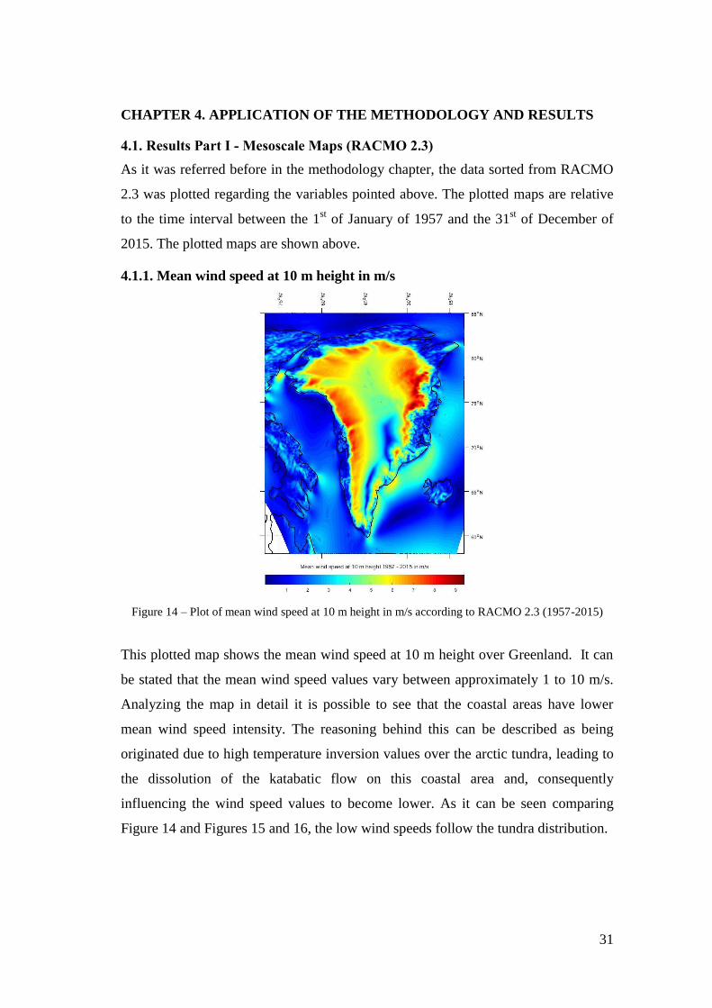
As it was referred before in the methodology chapter, the data sorted from RACMO
2.3 was plotted regarding the variables pointed above. The plotted maps are relative
to the time interval between the 1st of January of 1957 and the 31
st of December of
2015. The plotted maps are shown above.
4.1.1. Mean wind speed at 10 m height in m/s
Figure 14 – Plot of mean wind speed at 10 m height in m/s according to RACMO 2.3 (1957-2015)
This plotted map shows the mean wind speed at 10 m height over Greenland. It can
be stated that the mean wind speed values vary between approximately 1 to 10 m/s.
Analyzing the map in detail it is possible to see that the coastal areas have lower
mean wind speed intensity. The reasoning behind this can be described as being
originated due to high temperature inversion values over the arctic tundra, leading to
the dissolution of the katabatic flow on this coastal area and, consequently
influencing the wind speed values to become lower. As it can be seen comparing
Figure 14 and Figures 15 and 16, the low wind speeds follow the tundra distribution.

32
Figure 15 – Different biomes areas around the globe, Source: Grid Arendal, n.d.
Figure 16- Tundra in Greenland, zoomed in from previous Figure, Source: Grid Arendal, n.d
As we enter the ice sheet (GrIS) things change radically, the wind speed values
increase (less intense in the southern region and higher in the central region). This
can be explained by the semi-permanent katabatic flow that characterizes the wind
regime in the GrIS (Ettema et al., 2010 b).
The highest values can be seen over the northeast region. The climate in this area is
characterized by a rigorous winter with large volume of precipitation and high wind
speed values due to the cyclonic activity over the Greenland Sea, presented in this
area (Meltofte et al., 2008; Ettema et al., 2010b; Gorter et al. 2014), also refer the
presence of higher values of wind speed over the “Dronning Louise Land” (northeast
region), provoked by the rigorous winter with extremely cold temperatures combined
with the large terrain complexity resulting in higher wind speed values in their
simulations, although it is also mentioned that there are no direct observations for the
area.

33
4.1.2. Average maximum wind speed in m/s at 10 m height with (ffmax) /
without gusts (ffgmax)
Figure 17 – Plot of average maximum wind speed without gusts at 10 m height in m/s (ffmax)
according to RACMO 2.3 (1957-2015)
Figure 18 – Plot of average maximum wind speed with gusts at 10 m height in m/s (ffgmax)
according to RACMO 2.3 (1957-2015) Before explaining the resultant plots, average maximum wind speed as well as the
term gust will be defined. Both maximum wind speeds without gusts (ffmax) and

34
with gusts (ffgmax) refer to the maximum daily wind speed recorded. Consequently,
the average maximum wind speed can be understood as:
𝐴𝑣𝑒𝑟𝑎𝑔𝑒𝑑 𝑚𝑎𝑥𝑖𝑚𝑢𝑚 𝑤𝑖𝑛𝑑 𝑠𝑝𝑒𝑒𝑑 =1
𝑛 × ∑ 𝑢𝑚𝑎𝑥 (𝑖)
𝑛
𝑖=1
Equation 3 – Averaged maximum wind speed
Where:
umax = maximum wind speed in m/s
i = day (1 referring to 1st of January of 1957)
n = total number of days (58 years)
Gust is defined by the World Meteorological Organization (WMO) as “the maximum
wind averaged over 3 seconds interval”. ECMWF / RACMO use this as a gust
definition on its computation in order to be harmonious with the WMO (ECMWF,
2008).
As the two plots presented show a really similar distribution (however different
scaling) it was decided to show them in the same page. The average values of
maximum wind speed without gusts vary from 4 to 15 m/s and from 4-22 m/s with
gusts.
Analyzing the two plotted Figures 17 and 18, it is evident that there are two main
areas that present the maximum wind speed values: the southern area of Greenland,
Cape Farewell, and also an area on the southeast offshore area around 100 km
outside Mont Forel (3360 m of altitude) (Weidick et al., 1995).
Cape Farewell it is known for several years to be a dangerous path for maritime
transportation due to strength of the wind speed in the area. As an example, in 1959
the “MS Hans Hedtoft” ship collapse and with it 95 people died.
This high wind speeds are caused by the correlation between the complexity of the
terrain and the fact that Cape Farwell is located in an extra-tropical cyclones zone.
On the other hand the southeast region known by its steep terrain can produce a
channeling effect of the katabatic winds resulting in extremely high wind speed
values (Moore and Renfrew, 2014).

35
4.1.3. Mean temperature in K at 2 m height (T)
Figure 19 – Plot of mean temperature in K at 2 m height according to RACMO 2.3 (1957-
2015)
Evaluating the Figure 19, it is possible to understand that the temperature evolves
positively from the interior to the exterior of the ice sheet (GrIS). It can also be said
that the northern areas due to their high latitude values present generally colder
temperatures than the southern area. The coldest temperatures are registered in most
elevated point of the island, Gunnbjørn Fjeld, around 3700 m in East Greenland
(Greenland Statistics, 2015). The mean temperature levels fluctuate between 245 K
and 270 (aprox: – 28° C to – 3 °C).

36
4.1.4. Mean specific humidity in kg/kg at 2 m height (q)
Figure 20 – Plot of mean specific humidity in kg/kg at 2 m height according to RACMO 2.3
(1957-2015)
In this map we can definitely say that Greenland is notoriously dry. However by the
coast there some areas that presents slightly higher values for humidity, which varies
between 0 and 3 kg/kg. This can be justified by the presence of a semi-permanent
katabatic flow in the GrIS that transports dry air from the GrIS preventing the
increase of the humidity levels in the other parts of the island (Ettema et al., 2010 b).
Note: Temperature and humidity were not considered for the sites suggestions,
although both are extremely important to study the phenomena of icing occurrence
on wind turbines. This is one of the proposals for future work development.

37
4.1.5 Geopotential
Figure 21 - Geopotential according to RACMO 2.3 in dynamic height
The Geopotential can be defined as “the potential energy of a unit mass relative to
sea level, numerically equal to the work that would be done in lifting the unit mass
from sea level to the height at which the mass is located; commonly expressed in
terms of dynamic height (levels above mean sea level) or geopotential height”
(American Meteorological Society, 2012).
It is directly proportional to the elevation of the terrain, being represented by the
multiplication between the elevation values and the acceleration due to gravity.
RACMO 2.3 considers this value, g = 9,81665 m/s2.
38
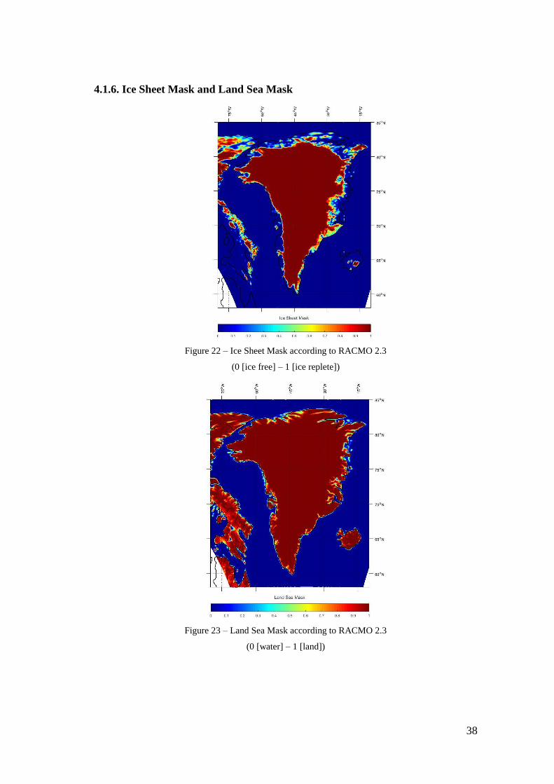
4.1.6. Ice Sheet Mask and Land Sea Mask
Figure 22 – Ice Sheet Mask according to RACMO 2.3
(0 [ice free] – 1 [ice replete])
Figure 23 – Land Sea Mask according to RACMO 2.3
(0 [water] – 1 [land])
39
The Figure 22 shows the Ice Sheet Mask, i.e., the representation of the continental
parts covered with ice in Greenland. It can be said that it is directly correlated with
the tundra map shown before (Figure 15/16), being the ice-free areas.
Figure 23, shows the Land Sea Mask, i.e., the continental area and sea area present in
Greenland. The areas in light read or yellow colors are parts of the continental shelf,
i.e., a relatively shallow water level that results from the extension of the land mass.
4.1.7. Combining mesoscale maps (mean wind speed & maximum wind speed)
In order to suggest possible deployment sites it was decided to look into areas with
suitable mean wind speed values avoiding at the same time high maximum values of
wind speed due to the possibility for occurrence of storms or “Piteraq” winds, which
could create high loads on the tower and blades that consequently conduct to longer
stoppages time due to maintenance operations or complete system damage. In
addition there is another issue: the turbine cut-off value that needs to be considered,
once the WTG will not produce over that wind speed. To verify the “optimum”
values of mean wind speed and maximum wind speed an assumption was created
considering the wind profile power law:
𝑣2 = 𝑣1 (ℎ2
ℎ1)
𝛼
Equation 4 – Wind profile power law
Where:
𝑣2 = projected speed at the desired height ℎ2
𝑣1 = observed speed at measurement height ℎ1
𝛼 = non-dimensional wind shear exponent
Table 2 below shows the 𝛼 values for different complexity of terrain and land cover.
Table 2 – non-dimensional wind shear exponents for various types of terrain and land cover
Source: Brower and Bailey, 2012

40
For the purpose of this project 𝛼 is assumed as 0,25, due to the tundra be considered
a low to moderate vegetation land cover and terrain type to be complex.
The turbines chosen for this project are Vestas V90 3MW (Vestas, n.d.) at 80 m
height (the specifications can be found in the appendix 4). The projected speeds (80
m height) based on the observed wind speeds (10 m height) are shown in table 3
below:
v1 [m/s] v2 [m/s] h1 [m] h2 [m] α
0 0 10 80 0,25
1 1,681793 10 80 0,25
2 3,363586 10 80 0,25
3 5,045378 10 80 0,25
4 6,727171 10 80 0,25
5 8,408964 10 80 0,25
6 10,09076 10 80 0,25
7 11,77255 10 80 0,25
8 13,45434 10 80 0,25
9 15,13614 10 80 0,25
10 16,81793 10 80 0,25
11 18,49972 10 80 0,25
12 20,18151 10 80 0,25
13 21,86331 10 80 0,25
14 23,5451 10 80 0,25
15 25,22689 10 80 0,25
16 26,90869 10 80 0,25
17 28,59048 10 80 0,25
18 30,27227 10 80 0,25
19 31,95406 10 80 0,25
20 33,63586 10 80 0,25
Table 3 – Wind speed at hub height according to the power law
In table 3 the values in blue delimit the mean wind speed values interval considered
as desirable for the project. The lower limit of mean wind speed was selected
according to the statement that “ utility-scale wind power plants require minimum
average wind speeds of 6 m/s” (European Commission, 2011). The upper limit was
set according to the maximum mean wind speed presented in the Figure 14 (10 m/s at
10 m height). The wind speed highlighted in the yellow cells shows the cut-off value
of the turbine according to turbine power curve. Taking this into consideration it can
be concluded that the values for mean wind speed will vary between 4 and 10 m/s at
10 m height, and maximum wind speeds higher than 14 m/s at 10m height should be

41
avoided. To have a better understanding of which are the areas of interest, a new
script based on the mean wind speed (UV) and average maximum wind speed
including gusts (ffgmax) plotting script was created (see example for ffgmax in
appendix 5) . This new feature consisted in isolating the desired data.
The results are shown in Figure 24.
Figure 24 – Plots considering limitations regarding mean wind speed and maximum wind speed
A combination between the two maps was performed. The goal was to find the best
correspondence between the mean wind speed and the average of maximum wind
speed limitations referred before.
Also it was requested to consider at least one site on the East coast. For the purpose
of the study three preliminary site suggestions can be found in table 4:
Preliminary Suggestions
Name Coordinates Mean ws Max ws Nearby towns* Location
Site suggestion 1
67° 45.000'N 48° 45.000'W
7 10 Sismut - 235 km
Kangerlussuaq - 120 km SW
Site suggestion 2
65° 36.000'N 49° 26.000'W
7 12 Nukk - 120 km
Kangerlussuaq - 165 km SW
Site suggestion 3
67° 0.000'N 35° 1.000'W
5 8 Kulusuk - 190 km SE
Table 4 - Preliminary Sites Suggestions
Table 4 shows the three site suggestions made (1,2,3), their coordinates, mean wind
speed and maximum wind speed as well as their location. The nearby towns are also

42
specified, although these values are approximated and measured in a straight line.
The suggested locations can be seen in Figure 25.
Figure 25 - Preliminary site suggestions
Even though according to table 4 the combination between mean and high wind
speed for site suggestion 1, 2 and 3 was within the set parameters (4-10 m/s for the
mean and lower than 14 m/s for maximum wind speeds), there were other factors that
arose from the choice of these site suggestions, which led to the idea of creating
project constraints before deciding about the locations for the micro-siting
examination.
4.1.8. Project Constraints
Although the wind speed can be plotted and used as the main guide for wind power
development, to advance with a feasibility study in the Greenlandic territory other
things should be taken into account. It is important to refer that no deep study
regarding geological conditions or grid connection availability was conducted during
this project, even though two factors were defined as project constraints:
Construction in the Greenlandic Ice Sheet (GrIS)
Proximity to towns or settlements

43
4.1.8.1. Construction in the Greenlandic Ice Sheet / Cap
The ice sheet/cap in Greenland (GrIS) covers more than 80% (see Figure 22) of its
territory (Greenland Statistics, 2015). It is the most extensive everlasting ice and
snow abounding zone in the North part of the globe (Ettema et al.,2010b). Therefore
it is important to assess if construction in the GrIS is possible. After some research it
was possible to understand that some construction does exist in the Ice Sheet. As an
example the “Summit Station”, located around 400 km from the Land Sheet, which is
a monitoring station for meteorological data (Summitcamp.org, 2016). There is no
data available regarding the specific details of construction from the “Summit
Station”, however it’s known that during the “Cold War” (1960) the US Army and
the Danish Government agreed on testing constructions under Artic Climate in order
to evaluate issues with mobile nuclear reactors as well as support scientific
investigation on the Ice Sheet. This agreement led to the creation of the “Century
Camp”. The installations entailed 26 ice tunnels, accommodation for 225 people,
storage facilities, labs for scientific investigation and a source of electricity
production by the means of a nuclear reactor. The reactor was installed in the same
year of the agreement however it was closed 3 years later due to problems with the
overall camp construction. The cause for this event was connected with the
inexistence of stability in the Ice Sheet caused by the constant movement instigated
by gravity. Also the foundations of the construction, mainly constituted by ice and
snow, played a major role on the disassembling of the camp.. The reasoning behind it
is related with these materials viscoelasticity properties, meaning that they tend to
deform due to atmospheric conditions and increased loads (Petersen, N., 2008).
After review it was decided that even if nowadays technology would permit
constructions on the Ice Sheet, this can be seen as extremely risky, and that the
suggested sites should be outside of the GrIS area.
4.1.8.2. Proximity to towns or settlements
As the main purpose of this study is to verify the feasibility of wind potential in
Greenland, it is important to take into consideration that most of the free-ice area is
inhabited. The population density is 0,14 per km2 (Greenland Statistics, 2015). As the
main cause to install wind power in the region is to provide electricity to users, the
potential increased price provoked by the extended length of transmission cables,
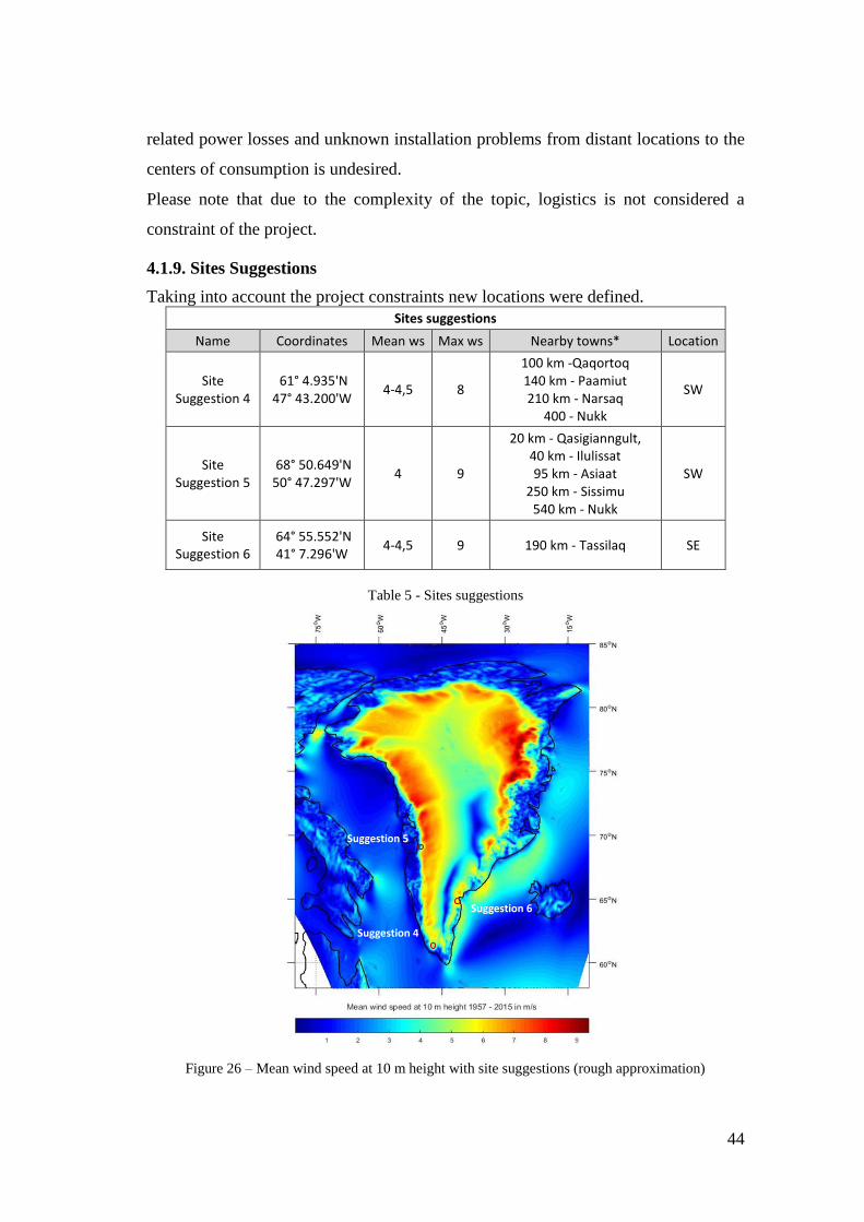
44
related power losses and unknown installation problems from distant locations to the
centers of consumption is undesired.
Please note that due to the complexity of the topic, logistics is not considered a
constraint of the project.
4.1.9. Sites Suggestions
Taking into account the project constraints new locations were defined.
Sites suggestions
Name Coordinates Mean ws Max ws Nearby towns* Location
Site Suggestion 4
61° 4.935'N 47° 43.200'W
4-4,5 8
100 km -Qaqortoq 140 km - Paamiut 210 km - Narsaq
400 - Nukk
SW
Site Suggestion 5
68° 50.649'N 50° 47.297'W
4 9
20 km - Qasigianngult, 40 km - Ilulissat 95 km - Asiaat
250 km - Sissimu 540 km - Nukk
SW
Site Suggestion 6
64° 55.552'N 41° 7.296'W
4-4,5 9 190 km - Tassilaq SE
Table 5 - Sites suggestions
Figure 26 – Mean wind speed at 10 m height with site suggestions (rough approximation)
Suggestion 5
Suggestion 4
Suggestion 6

45
Just as an observation the population of the referred nearby towns is shown:
Site suggestion 4:
Qaqortoq, population 3229 (2013)
Paamiut, population 1515 (2013)
Narsaq, population 1503 (2013)
Nukk, population 16.583 (2013)
Site suggestion 5:
Qasigianngult, population 1171 (2013)
Ilulissat, population 4541 (2013)
Asiaat, population 3102 (2013)
Sissimut, population 5598 (2013)
Nukk, population 16.583 (2013)
Note 1: The sum of these populations is equal to 55 % of the Greenlandic population
(including Nuuk) and 25,5% (excluding Nukk)
Site Suggestion 6:
Tassilaq, population 2017 (2013)
(Greenland Statistics, 2013)
Note 2: It was difficult to identify if site suggestion 5 and site suggestion 6 were in
fact outside the Ice Sheet. This question was made to IMAU when the data regarding
the coordinates was sent. IMAU responded that is generally accepted that Google
Earth does not commit mistakes in geolocation therefore, it could be concluded that
all site suggestions were outside the GrIS (van de Berg).
As all locations are situated in the southern part of the island, the northern area is not
shown in the final suggestions map (Google Earth version).

46
Figure 27 – Final Site Suggestions, Source: Google earth
Having the site suggestions selected, the multi-level data was requested and Part II of
the project initiated.
4.2. Results PART II – Micro-scaling Analysis
4.2.1. Grid Independence – Results Site Suggestions 4,5 and 6
The results for mean wind speed at 80 meters height, for site suggestions 4,5 and 6
for the full terrain domain interpolated by WindSim from the data acquired from the
climatology at 70 m, as well as its convergence can be seen in Figure 28 and 29:
Figure 28- Mean Wind Speed [m/s] at 80 m site suggestions 4,5 and 6 for full terrain domain
5
5,25
5,5
5,75
6
6,25
6,5
6,75
7
7,25
7,5
500 1000 1500 2000 2500 3000 3500 4000
U m
ean [
m/s
]
Number of Cells * 103
Umean 80 m Site Suggestion 4,5,6
Suggestion 4
Suggestion 5
Suggestion 6
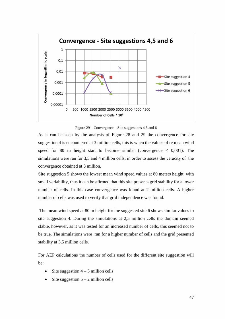
47
Figure 29 – Convergence – Site suggestions 4,5 and 6
As it can be seen by the analysis of Figure 28 and 29 the convergence for site
suggestion 4 is encountered at 3 million cells, this is when the values of te mean wind
speed for 80 m height start to become similar (convergence < 0,001). The
simulations were ran for 3,5 and 4 million cells, in order to assess the veracity of the
convergence obtained at 3 million.
Site suggestion 5 shows the lowest mean wind speed values at 80 meters height, with
small variability, thus it can be afirmed that this site presents grid stability for a lower
number of cells. In this case convergence was found at 2 million cells. A higher
number of cells was used to verify that grid independence was found.
The mean wind speed at 80 m height for the suggested site 6 shows similar values to
site suggestion 4. During the simulations at 2,5 million cells the domain seemed
stable, however, as it was tested for an increased number of cells, this seemed not to
be true. The simulations were ran for a higher number of cells and the grid presented
stability at 3,5 million cells.
For AEP calculations the number of cells used for the different site suggestion will
be:
Site suggestion 4 – 3 million cells
Site suggestion 5 – 2 million cells
0,00001
0,0001
0,001
0,01
0,1
1
0 500 1000 1500 2000 2500 3000 3500 4000 4500
Co
nve
rge
nce
in lo
gari
thm
ic s
cale
Number of Cells * 103
Convergence - Site suggestions 4,5 and 6
Site suggestion 4
Site suggestion 5
Site suggestion 6
48
Site suggestion 6 – 3,5 million cells
4.2.2. AEP determination
To determine the AEP for the 3 different proposed sites, the turbine Vestas V90
3MW with an 80 m hub height was selected. This particular choice was made in
order to understand and compare results for the different sites in a normalized way,
but also due to the fact that the application of this turbines model worldwide is rather
common. Subsquent studies should be conducted to understand if this is the most
adequate turbine for this specific weather conditions, however, for the scope of this
project, as the main goal is to understand the feasibility of wind power in Greenland
in terms of wind resource assessment the turbine selection was not one of the
analysis performed.
To calculate the AEP, the wind resource map at 80 m was studied for each site, and
the best wind resource locations selected. The study was performed with 3 turbines
Vestas V90 3MW, and the AEP for each suggested site compared and analyzed.
A discussion regarding different values obtained from the different climatology
heights (10, 35, 70, 100 and 120 m) interpolated for hub height (80 m)was also
executed. Important to note that this is not part of the project’s scope, but as it is an
interesting finding is shown on the thesis.

49
4.2.2.1. Site suggestion 4 – results
As it was said before, the wind resource map was examined and the locations that
presented better results were elected.
Figure 30 – Wind Resource map at 80 m (Site suggestion 4)
In Figure 30, the wind resource distribution at 80 m interpolated by WindSim from
the climatology file at 70 m height for the suggested site 4 is represented.
The grey circle represents the virtual met mast created at different heights (10, 35,
70, 100 and 120 m), according to the multi-level data provided by IMAU, located at
the site center and the triangles represent positioned wind turbines (Vestas V90 3MW
at 80 m hub height). As it can be seen the positions for the wind turbines show a
mean wind speed between 10 and 12.5 m/s. Important also to refer that no wake
interference was considered.
Assuming these positions as the best wind resource possible the AEP was calculated,
and the following results according to the Weibull distribution are represented in
Figure 31 and shown in table 6:
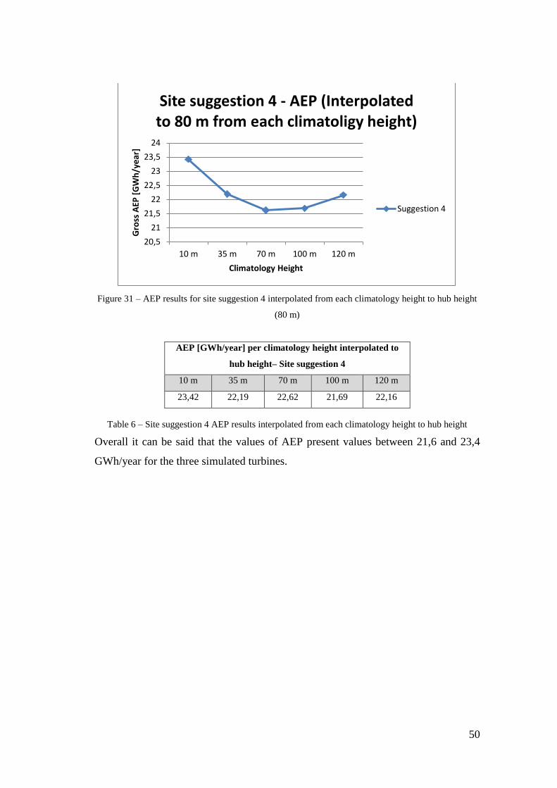
50
Figure 31 – AEP results for site suggestion 4 interpolated from each climatology height to hub height
(80 m)
AEP [GWh/year] per climatology height interpolated to
hub height– Site suggestion 4
10 m 35 m 70 m 100 m 120 m
23,42 22,19 22,62 21,69 22,16
Table 6 – Site suggestion 4 AEP results interpolated from each climatology height to hub height
Overall it can be said that the values of AEP present values between 21,6 and 23,4
GWh/year for the three simulated turbines.
20,5
21
21,5
22
22,5
23
23,5
24
10 m 35 m 70 m 100 m 120 m
Gro
ss A
EP [
GW
h/y
ear
]
Climatology Height
Site suggestion 4 - AEP (Interpolated to 80 m from each climatoligy height)
Suggestion 4

51
4.2.2.2. Site suggestion 5 – results
The process followed to achieve the AEP results for site suggestion 5 is similar as the
one taken to achieve the results for site suggestion 4. In Figure 32 the wind resource
distribution at 80 m interpolated by WindSim from the climatology file at 70 m
height for the suggested site 5 is represented.
Figure 32 – Wind Resource map at 80 m (Site suggestion 5)
By examining the result of the wind resources map for this site suggestion it is
possible to see that the site does not present a high overall mean speed. The best wind
resource positions (where the turbines were inserted) show wind speed on the order
of 6,5 m/s, however, the terrain shows to be relatively homogeneous, i.e., most of the
existent wind resources values are situated between 5 and 6 m/s. The calculated AEP
is represented in Figure 33 and shown in table 7:

52
Figure 33 – AEP results for site suggestion 5 interpolated from each climatology height to hub height
(80 m)
AEP [GWh/year] per climatology height interpolated to
hub height – Site suggestion 5
10 m 35 m 70 m 100 m 120 m
18,85 14,73 12,08 10,96 10,52
Table 7 – Site suggestion 5 AEP results interpolated from each climatology height to hub height
As expected by analyzing the wind resource map, the interpolated AEP for this site
suggestion is lower than the one achieved for site suggestion number 4, presenting
production results from 10,5-18,9 GWh/year.
0
5
10
15
20
10 m 35 m 70 m 100 m 120 m
Gro
ss A
EP [
GW
h/y
ear
]
Climatology Height
Site suggestion 5 - AEP (Interpolated to 80 m from each climatology height)
Suggestion 5

53
4.2.2.3. Site Suggestion 6 – results
As said before, the results obtainment followed a standardized process. In Figure 34
the wind resource distribution at 80 m interpolated by WindSim from the climatology
file at 70 m height for the suggested site 6 is represented.
Figure 34 – Wind Resource map at 80 m (Site suggestion 6)
Site suggestion 6 shows a high wind speed distribution namely on the northeast and
southwest of the site. The turbines were positioned in the higher wind resources
areas, approximately 9-10, 5 m/s. It is important to refer that according to IMAU this
site is the one in which the wind output from the RACMO system can be less
representative due to local effects that can be significant subsequently affecting the
data.
The calculated AEP is represented in Figure 35 and shown in table 8:

54
Figure 35 – AEP results for site suggestion 5 interpolated from each climatology height to hub height
(80 m)
AEP [GWh/year] per climatology height interpolated to
hub height – Site Suggestion 6
10 m 35 m 70 m 100 m 120 m
18,55 18,24 17,54 16,97 16,88
Table 8 – Site suggestion 5 AEP results interpolated from each climatology height to hub height
The calculated AEP for site suggestion 6, shows values between 16,9 – 18,6
GWh/year for the different climatology heights when interpolated to hub height.
16
16,5
17
17,5
18
18,5
19
10 m 35 m 70 m 100 m 120 m
Gro
ss A
EP [
GW
h/y
ear
]
Climatology Height
Site suggestion 6 AEP (Interpolated to 80 m from each climatology height)
Suggestion 6

55
4.2.3 . AEP comparison
In order to evaluate which would be the best site for turbine deployment according to
the micro scaling analysis exercise performed, data from the obtained AEP for the
different sites suggestions was compared.
The results show different AEPs for different climatology heights (Figure 36).
Figure 36 Interpolated AEP (80 m) results for all site suggestions according to different climatology
heights
After understanding that results show a variability according to the climatology
height it was decided that the AEP for the climatology at 70 m interpolated to the hub
height was the most representative, once it was the closest to the simulated turbines
hub height (Vestas V90 3MW at 80 m), and interpolation errors would be smaller.
A plot with the different AEPs for the 3 different sites suggestions at hub height,
concerning the data provided exclusively by the climatology at 70 m is shown in
Figure 37.
0
5
10
15
20
25
10 35 70 100 120
AEP
[G
Wh
/ye
ar]
Climatology Heights [m]
AEP interpolated at 80 m from different climatology heights
[GWh/year]
Site suggestion 4
Site suggestion 5
Site suggestion 6

56
Figure 37 – AEP results for all site suggestions with data from climatology at 70 m interpolated to hub
height
By examining Figure 37, it can be concluded that site suggestion 4, is the site
suggestion that presents higher values of AEP, showing an increase of 79,02% and
23,26 % when compared to site suggestion 5 and 6 respectively. The results are
based on both climatology data at 70 m interpolated to hub height and positions of
highest wind speed value.
Note: From data inputted in “Windographer” it was possible to obtain the wind
profiles for the different sites suggestions (4, 5 and 6) as well as the trends of mean
wind speed variation from each climatology data (at the climatology position)
according to each month, showing that wind speed is higher during the winter period
(November to April), as previously discussed. This is presented in appendix 8.
0
5
10
15
20
25A
EP a
t h
ub
he
igh
t in
terp
ola
ted
fro
m
clim
ato
logy
at
70
m [
GW
h/y
ear
]
Comparison of interpolated AEP based on 70 m climatology all
site suggestions
Site suggestion 4
Site suggestion 5
Site suggestion 6

57
CHAPTER 5. DISCUSSION AND ANALYSIS
5.1. Part I
RACMO 2.3 is a model that can provide relevant information regarding wind
resources and other weather properties in Greenland, both due to the small grid
resolution when compared to other similar models (±11 km) as well as to the large
size sample of data collected every 6 hours from 1957-2015.
The output data analyzed from the mesoscale simulations is in accordance with
studies presented using RACMO2.1 As an example in Ettema et al., 2010b) the mean
wind speed map at 10 m height is similar to the result of this study. The only stated
incoherence is the plotted data for the wind speed offshore. This can be justified
because Ettema et.al, 2010b) considers the vector length of the winds, as in this study
the vector composition of mean wind were represented.
Maps regarding other characteristics were also plotted. Features such as temperature,
humidity, Ice Sheet Mask, Land Sea Mask and Geopotential can be observed,
however they had not a direct influence in the project development.
The results from the mesoscale simulations (maps) are an excellent tool to wind
power developers potentially interested in Greenland. Nevertheless, it is important to
refer that a mesoscale map gives only a rough idea of potential sites for construction,
and further analysis needs to be made.
5.2. Part II
Micro-scaling in Greenland can be challenging, both because of the orographic
complexity but also due to the difficulty in finding specific tools such as maps with
good information on height contours and roughness resolution.
Site suggestion 4 was the one that shows to be the most suitable for wind power
deployment, from the three presented suggestions. However according to the wind
resource map (Figure 30), it seems that the wind distribution at this site is diverse,
varying from areas with 2,5 m/s to 10 m/s and where the highest wind speed values
positions are few. Therefore, if a utopic project consists in constructing a large wind
farm the conclusion that this suggested site is the most valuable option can be false.
58
In fact, it does possess the highest AEP values from the 3 chosen deployment sites,
but, the wind distribution is generally heterogeneous.
Site suggestion 5 seemed to be a valuable wind site option according to the analysis
of the mesoscale maps (Figure 32). However, after the data at different levels was
provided by RACMO 2.3 the analyzed information did not presented high wind
speed values.
This is a good example of some inaccuracy of mesoscale maps, i.e., they can be used
as a tool to provide a rough idea of the wind resources in a particular site; however
they can mislead the developer, particularly if the chosen site is in the border
between a low and a higher wind speed area. This was in fact the issue with site
suggestion 5 once it is located near the coastline where the wind resources are
extremely low, and a small difference in the coordinate’s values moved this
suggested site to the lower wind resource area.
Site suggestion 6, on other hand, has the second highest value of AEP, not too distant
from the results presented for site 4. Besides the stated AEP values, it also presents a
stable variability of wind speed values (Figure 34), mostly within the area between 6
and 8 m/s, which is a “good” trend for wind power development, especially if a
utopic large wind farm is projected.
Nevertheless, as it was stated before, according to IMAU, the RACMO 2.3 model
can be less representative in this case due to its inhomogeneity, hence rough terrain,
which can conduct to misleading values of wind speed. Even though the height
contour lines show a good distribution in the map, the same does not happen with
roughness. This characteristic based on the WindPro database shows a poor
distribution if compared with the other site suggestions. It is possible that the
roughness data is inaccurate, although it was not possible to find anything that proves
the contrary. This poor distribution can enhance the homogeneity of wind speed in
the area.
Based on the analysis performed for each site suggestion, it can be said that site
suggestion 4, both for its high AEP results and for being relatively close to populated

59
areas, would be the site with higher potential for wind power development. This
conclusion can be achieved when compared with site suggestion 5 and 6:
Site suggestion 5 presents the lowest AEP results, even though it is the closest site to
populated areas. As it was mentioned before, IMAU provided data from the nearest
RACMO grid point accordingly to the coordinates provided by the author. The site,
according to the mesoscale map is located between two different wind speed areas (3
and 4 m/s). This means that a difference between the coordinates provided and the
nearest grid point can lead to a lower wind speed area. IMAU informed that for the
reason stated above, data for a different grid point could be provided for results
improvement.
Site suggestion 6 presents the middle value of AEP and a homogeneous wind speed
distribution. However it is pointed by IMAU as having the possibility to present
inaccurate data due to modelling difficulty, the uncertainty regarding the detail of the
roughness on the outputted map, as well as being located in a remote area where the
nearest population is about 180 km away.
Analyzing the mean wind profile for site suggestion 4 (Figure 39 in appendix 8), it
can be stated that at 80 m height the mean wind speed is higher than 7 m/s. This
shows a capacity factor ≈ 29%, which is considered relatively good for wind power
development onshore as the average capacity for onshore wind turbines in Europe
according to EWEA (2011) is 24 %.
Particularizing, the potential for wind power development in Greenland presents
better results if compared, for example, with the data obtained from the NREL, at 80
m height in the state of California, in the USA, where 2 wind farms, Hatchet Ridge
Wind Farm and Walmart Red Bluff Wind Farm, had been developed in 2010 and
2012 respectively, in the proximity of Redding (Figure 46) and where the mean wind
speed at 80 m height vary between 5,5 and 6 m/s (Figure 45) (NREL, 2010). Figure
45 and 46 used for this comparison are presented in appendix 9.
Besides site suggestion 4, there are other sites that present high potential for wind
power development. The southwest region shows higher mean wind speeds when

60
compared with the southeast. This fact can boost wind power once the most
populated areas in Greenland are located in the southwest region.

61
CHAPTER 6. CONCLUSIONS
To understand the feasibility of wind power utilization in Greenland a study was
conducted. The data used for project development was provided based on RACMO
2.3 (Regional Atmospheric Climate Model), specially improved for arctic climate by
the Institute of Marine and Atmospheric Research of Utrecht University (IMAU).
The provided data contained information about various parameters such as: wind
speed, maximum wind speed with and without gusts, temperature and humidity for
the time stamp of 1957 – 2015.
The acquired data was processed and a script was developed in Matlab in order to
obtain mesoscale maps regarding the different features as an output.
The mesoscale maps showed that Greenland is affected by different wind speeds,
being the coastal area the one presenting lower mean wind speed values (2-3 m/s).
On the other hand areas in the boundaries of the ice sheet as well as the elevated
regions were the ones presenting higher wind speeds (6-9 m/s).
By analyzing the map concerning the average maximum wind speed it was also
possible to observe that in some regions this value is high, therefore not so effective
for wind power utilization.
The mean wind speed and maximum wind speed maps were combined, and three
sites were initially proposed for further analysis (suggestion sites 1, 2 and 3). It is
important to refer however, that proximity to towns and settlements, as well as the
great extent of the Greenlandic Ice Sheet had to be taken into account and therefore
constraints to the project were set.
According to the constraints described above, three new sites were chosen to perform
a micro-scale analysis (sites suggestion 4, 5 and 6).
Data regarding height contours and roughness were found in WindPro online
databases and maps of the chosen areas generated. Converting the output data a
terrain file was created in WindSim.
As RACMO 2.3 data provided by IMAU concerning wind speed was given
previously at 10 m height for all the Greenland territory, new data was requested in
order to assess the wind resource assessment in the specific locations. This data
included wind speed at different levels (10, 35, 70, 100 and 120 m) for the interval
from 1958 to 2015 every 6 hours. A new script was then developed in Matlab with

62
the main goal of creating files with data sorted by type: date, wind speed and wind
direction. Climatology files were generated based on the sorted information for
WindSim input.
The acquired data was simulated in WindSim, and the micro-scale simulations
performed for each one of the suggested sites.
The AEP was calculated assuming the best wind resources positions for three
turbines Vestas V90 3MW at 80 m hub height. The data used to attain the results is
based on an interpolation performed from the data of the climatology at 70 m (closest
to the hub height) interpolated to the hub height.
Interpolation from different climatology heights to 80 m revealed different AEP
outputs. The main factor affecting these results is the fact the interpolation factor
used for lower climatology heights is higher than the one used by the software for
higher heights. However this is not evaluated in depth in the current report as it is not
part of the project’s scope.
Results showed that the site presenting higher interpolated AEP values for the pre-
determined conditions was site suggestion 4 surpassing in 79,0% and 23,3 % the
production results from site suggestion 5 and 6 respectively.
Even though the project possesses a large number of limitations, in a general manner
it can be said that Greenland has in fact potential for wind power development based
on wind resource assessment.

63
6.1. Limitations and Future Work
As the main focus of this study was only wind resource assessment important areas
such as logistics, grid connection and stability, icing related problems, finance,
policies, planning or permissions for wind energy were not taken into account. To
develop a complete feasibility study the areas cited above should be investigated.
Some tools created during this research, such as humidity and temperature maps, can
assist the development of a detailed study regarding other characteristics, such as
icing for example.
The request for multi-level data originated the creation of a new script by IMAU that
allows creating multi-level data for all the RACMO grid points. As it was pointed out
before supplementary data can be requested for future studies.
The multi-level data obtained from RACMO 2.3 for the three site suggestion is
modeled from the nearest grid point to the coordinates provided to IMAU when
multi-level data was requested. Therefore the site data is an approximation of what it
can in reality, once it is possible to understand that the terrain complexity has a high
effect on micro-scaling exercises.
A study of the RACMO 2.3 model’s accuracy was not performed.
To be able to obtain the level of uncertainty of the model, the provided data should
be confronted with real met mast data.
Maps, height contours and roughness were extracted via WindPro.
Although this process is one of the possible ways, accurate mapping data, for
example provided by the Danish/Greenlandic governments could be a huge
improvement to this study, as it will certainly provide detailed information that it is
not possible to acquire by using WindPro databases.
As an example, it can be said that in the obtained map for site suggestion 6 obtained
via WindPro, even though roughness and height contours information was inputted, it
seemed to be insufficient for a complete site analysis.

64
The different results from AEP interpolated for hub height from different climatology
heights could be analyzed in detail. This would conduct to a better understanding of
the reasons behind the results variations.
The simulations performed in WindSim were executed using “a virtual” met mast.
This was the path found in order to be able to input the climatology data. However, if
the goal is to obtain a detailed study of a particular site, real measures need to be
executed, for a period no less than 2 years. This is done so results will account for
season variability and provide lower uncertainty.
Furthermore the area for deployment could be refined and a detailed study could be
conducted.
It can be also interesting to analyze the possibility for wind power developing in
isolated settlements. This will provide them with electricity from a green source of
energy as well as energy independency.

65
REFERENCES
American Meteorological Society, 2012, “Glossary of meteorology – Geopotential”
[Online]
Available from: http://glossary.ametsoc.org/wiki/Geopotential
Accessed [14th
July, 2016]
Baunbaek, L. (2014), ”Grønlands energiforbrug” 2013 Grønlands Statistik
Bjarnason, Bjarni (2007), “Aluminium and Power in Iceland and Greenland”
Brower, Michael and Bruce H Bailey. Wind Resource Assessment. Hoboken, N.J.:
Wiley, 2012. Print.
Cappelen, J., Jørgensen, B., Laursen, E., Stannius, L. and Thomsen, R. (2001). The
Observed Climate of Greenland, 1958-99 - with Climatological Standard
Normals, 1961-90. Technical Report 00-18. Copenhagen 2001: Danish
Meteorological Institute - Ministry of transport, pp.21-32.
Dragsted, J. (2011). Solar heating in Greenland . Resource assessment and potential.
Ph.D. DTU - Civil Engineering Report R-240.
Earthobservatory.nasa.gov. (2016). Global Maps. [online]
Available from:
http://earthobservatory.nasa.gov/GlobalMaps/view.php?d1=CERES_NETFLU
X_M)
[Accessed 25th
July, 2016]
ECMWF (2008), IFS Documention – CY33r1 – Part IV: Physical processes
Emd, n.d. Emd
Available from: http://www.emd.dk/windpro/
Accessed: [7th
July, 2016]
ESMAP (2010), Best Practice Guidelines for Mesoscale Wind Mapping Projects for
the World Bank
Ettema, J., van den Broeke, M., van Meijgaard, E., van de Berg, W., Box, J. and
Steffen, K. (2010a). Climate of the Greenland ice sheet using a high-resolution
climate model – Part 1: Evaluation. The Cryosphere, 4(4), pp.511-527.
Ettema, J., van den Broeke, M., van Meijgaard, E. and van de Berg, W. (2010b).
Climate of the Greenland ice sheet using a high-resolution climate model – Part
2: Near-surface climate and energy balance. The Cryosphere, 4(4), pp.529-544.
European Comission (2011) - 2011 Technology Map of the European Strategic
Energy Technology Plan (SET-Plan)
EWEA, 2011 – Wind Energy Statistics and Targets – Fact sheet [Online]
Available from:
http://www.ewea.org/fileadmin/files/library/publications/statistics/Factsheets.p
df
Accessed [12th
October 2016]
Gorter, W., van Angelen, J., Lenaerts, J. and van den Broeke, M. (2013). Present and
future near-surface wind climate of Greenland from high resolution regional
climate modelling. Clim Dyn, 42(5-6), pp.1595-1611.
Greenland in Figures 2013, 10th
revised edition pp.21, March 2013
Statistics Greenland
Greenland in Figures 2015, 12th
revised edition pp.24, March 2015, Statistics
Greenland
Grid Arendal, n.d., “Tundra”
66
Available from: http://www.grida.no/graphicslib/detail/tundra_1338#
Accessed [14th
July, 2016]
Grobe, H., Wegener Alfred (2007), “Sketch about the two forces, pressure gradient
and gravitation force, producing Katabatic Wind at the margin of an ice sheet
or glacier”, Institute for Polar and Marine Research, Bremerhaven, Germany
GWEC, 2015, “Annual installed global capacity 2000-2015” Global Wind Energy
Council [Online]
Available from: http://www.gwec.net/global-Figures/graphs/
Accessed [2nd
September, 2016]
Harden, B., Renfrew, I. and Petersen, G. (2011). A Climatology of Wintertime
Barrier Winds off Southeast Greenland. Journal of Climate, 24(17), pp.4701-
4717.
Landsvirkjun Power, 2016, Sisimiut Hydropower Project
Available from: http://www.lvpower.com/Projects/Sisimiut/
Accessed: [10th
July 12, 2016]
Lenaerts, J. T. M., van den Broeke, M.R., van Angelen, J. H., van Meijgaard, E., and
Déry, S. J., 2012 "Drifting Snow Climate Of The Greenland Ice Sheet: A Study
With A Regional Climate Model". The Cryosphere 6.4, 891-899.
Lepparanta, Matti, 2005, The Drift Of Sea Ice, Springer, Berlin
Lyck, Lise and Jørgen Taagholt, 1986. "Greenland - Its Economy And Resources".
ARCTIC 40.1, no. 1, pp. 50-59
Mahrt, L., 1982. Momentum balance of gravity flows. J. Atmos.
Sci., 39(12), pp. 2701-2711.
Mathiot, P., Barnier, B., Gallée, H., Molines, J., Sommer, J., Juza, M. and Penduff,
T. (2010). Introducing katabatic winds in global ERA40 fields to simulate their
impacts on the Southern Ocean and sea-ice. Ocean Modelling, 35(3), pp.146-
160.
Meissner, C., 2010. WindSim, Getting Started. WindSim 5. 5th
edition
Meltofte, Hans, Torben R Christensen, and Bo Elberlong, ”High-Artic Ecosystem
Dynamics in a Chaniging Climate”, Burlington: Elsevier, 2008, Print
Moore, G. and Renfrew, I. (2005). Tip Jets and Barrier Winds: A QuikSCAT
Climatology of High Wind Speed Events around Greenland. Journal of
Climate, 18(18), pp.3713-3725.
Moore, G.W.K. and Renfrew, I.A., 2014, “A new look at Southeast Greenland barrier
winds and katabatic flow”- Contribution to U.S. Clivar Newsletter
Nilsson, K., 2010. Estimation of wind energy production in relation to orographic
complexity – A reliability study of two conventional computer software. Gotland
University
Noël, B., Van De Berg, W. J., Van Meijgaard, E., Kuipers Munneke, P., Van De
Wal, R. S W, Van Den Broeke, M. R. (2015). Evaluation of the updated
regional climate model RACMO2.3 : Summer snowfall impact on the
Greenland Ice Sheet
The Cryosphere, volume 9, issue 5, pp. 1831 - 1844
Nukissiorfiit, 2013, “Årsberetning 2013”
Petersen, Nikolaj, 2008, "The Iceman that Never Came". Scandinavian Journal of
History 33.1 pp.75-98.
67
Smits, Coco C.A., Jens Christian S. Justinussen, and Rasmus G. Bertelsen (2016),
"Human Capital Development And A Social License To Operate: Examples
From Arctic Energy
Stull, Roland, R.B, (2009) “An Introduction to Boundary Layer Meteorology:
Atmospheric and Oceanographic Sciences Library”, Volume 13, Springer
Summitcamp.org. (2016). summit. [online] Available at:
http://www.summitcamp.org/ [Accessed 14th
July, 2016].
The Nordic Council of Ministers - Facts about Greenland, 2016 [Online]
Available from:
http://www.norden.org/en/fakta-om-norden-1/the-nordic-countries-the-faroe-
islands-greenland-and-aaland/facts-about-greenland
[Accessed 8th
June 19, 2016]
Undén, P., Rontu, L., Jãrvinen, H., Lynch, P., Calvo, J., Cats, G., Cuxart, J., Eerola,
K., Fortelius, C., Garcia-Moya, J.A., Jones, C., Ldenderlink, G., Mcdonald, A.,
Mcgrath, R., Navascues, B., Nielsen, N.W., Degaard, V., Rodriguez, E.,
Rummukainen, M., Sattler, K., Sass, B.H., Savijarvi, H., Schreur, B.W., Sigg,
R., and The, H. (2002). HIRLAM-5, Scientific Documentation, Technical
Report
Unidata, n.d. , “What is a NetCDF file”
Available from: http://www.unidata.ucar.edu/software/netcdf/docs/faq.html
Accessed: [7th
July 12, 2016]
van Angelen, J. H., M. R. van den Broeke, and W. J. van de Berg, 2011, "Momentum
Budget Of The Atmospheric Boundary Layer Over The Greenland Ice Sheet
And Its Surrounding Seas". J. Geophys. Res. Vol. 116.D10, pp.1-14
van As, D., Fausto, R.S., Steffen, K., Ahlstrom, A.P., Andersen, S.B. , Andersen,
M.L., Box, J.E., Charalampidis, C., Citterio, M, Colgan, W.T, Edelvang, K,
Larsen, S.H., Nielsen, S., Veicherts, M. and Weidick, A.(2014). Katabatic
winds and piteraq storms: observations from the Greenland ice sheet
van de Berg, Willem Jan. RACMO 2.3 GREENLAND CLIMATE RUNS PROJECT
- Sites Suggestions. 2016. E-mail.
van den Broeke, M.R., Duynkerke, P.G. & Oerlemans, J., 1994. The observed
katabatic flow at the edge of the Greenland ice sheet during GIMEX-91. Global
and Planetary Change, 9(1-2), pp.3–15.
van den Broeke, M. and Gallée, H. (1996). Observation and simulation of barrier
winds at the western margin of the Greenland ice sheet. Q.J Royal Met. Soc.,
122(534), pp.1365-1383.
van Wessem, J.M., Reijmer, C.H., Lenaerts, J.T., van de Berg, W.J., van den Broeke,
M.R., and van Meijgaard, E. (2014). Updated cloud physics in a regional
atmospheric climate model improves the modelled surface energy balance of
Antarctica, The Cryosphere,8, pp. 125-135
Vestas, 2016, “Vestas V90 3MW – Techincal Specifications”
Available from: https://www.vestas.com/en/products/turbines/v90-
3_0_mw#!technical-specifications
Accessed [15th
July, 2016]
Weidick, Anker, Richard S Williams, and Jane G Ferrigno, 1995, “Satellite Image
Atlas Of Glaciers Of The World. Washington: United States government
printing office” Print.
WaSP, n.d.WaSP

68
Available from: http://www.wasp.dk/
Accessed: [7th
July 12, 2016]
WindSim, n.d. WindSim [Online]
Available from: http://www.windsim.com
Accessed: [7th
July 12, 2016]
Wilson, Emma (2015), “Energy and minerals in Greenland: governance, corporate
responsibility and social resilience”. 2nd
Edition, London
Zhang, Matthwe Huaiquan, “Wind Resource Assessment and Micro-Siting”. 1st
Edition, Wiley

69
APPENDIX 1 - Script for data sorting (example meridional mean wind speed V)
clear all; close all; clc % Insert netcdf toolbox javaaddpath('C:\Users\josda921\Desktop\Matlab\netcdfAll-4.3.jar') addpath('C:\Users\josda921\Desktop\Matlab\mexcdf.r4053\mexcdf\snctoo
ls') addpath('C:\Users\josda921\Desktop\Matlab\mexcdf.r4053\mexcdf\mexnc'
) addpath('C:\Users\josda921\Desktop\Matlab\netcdf_toolbox\netcdf_tool
box') % Define decades (Files)
II=[1957 1961 1971 1981 1991 2011]
for l=1:length(II) m=II(l); % Get V, lat, lon, time, height filename=sprintf('v10m.%.4i.nc', m); v_lat=ncread(filename,'lat'); v_lon=ncread(filename,'lon'); vt=ncread(filename,'dtg'); vh=ncread(filename,'height'); % Dimensioning V=ncread(filename,'v10m'); % %Regriding [dim_x dim_y]=size(v_lat); % [dim_z dim_a]=size(v_lat); V_y= zeros(dim_x,dim_y,length(vh),length(vt));
for i=1:size(vt) % time u i for j=1:size(vh) % heights (the same for both files) % Get V combined V_y(:,:,j,i)=griddata(double(v_lat),double(v_lon),double(squeeze(V(:
,:,j,i))),double(v_lat),double(v_lon)); end end % Name files according to data
eval(['v_lat' num2str(II(l)) '=v_lat;']); eval(['v_lon' num2str(II(l)) '=v_lon;']); eval(['vh' num2str(II(l)) '=vh;']); eval(['vt' num2str(II(l)) '=vt;']); eval(['V_y' num2str(II(l)) '=V_y;']);
% Save *.mat files and clear 4D arrays
writefile=sprintf('v.%.3i.mat', II(l)); clear v_lat v_lon vh vt V_y V; save( writefile,'-v7.3'); clear v_lat* v_lon* vh* vt* V_y*; end

70
APPENDIX 2 (Plotting – Example - UV)
% U (x component)
II=[1957 1961 1971 1981 1991 2011]
for l=1:length(II) m=II(l); % Get U combined + years sum filename = sprintf('u.%.4i.mat', m); load (filename,'U_x*') med_u = sprintf('U_x%.4i',m); A = eval(med_u); U = sum(A,4); eval(['U' num2str(II(l)) '=U;']); clear u_lat* u_lon* u_h* U_x* med_u A; end
% final sum (t.2001 has other name, first file converted) load u.2001.mat; U2001=sum(U_x,4); yr_total = 1218+3652+3653+3652+3653+3652+1826; U_all=(U1957+U1961+U1971+U1981+U1991+U2001+U2011)/yr_total;
% Clean 4D arrays
clear U_x uh ut
% V (y component)
II=[1957 1961 1971 1981 1991 2011]
for l=1:length(II) m=II(l);
% Get V combined + years sum filename = sprintf('v.%.4i.mat', m); load (filename,'V_y*') med_v = sprintf('V_y%.4i',m); B = eval(med_v); V = sum(B,4); eval(['V' num2str(II(l)) '=V;']); clear v_lat* v_lon* v_h* V_y* med_v B; end
% final sum (t.2001 has other name, first file converted) load v.2001.mat; V2001=sum(V_y,4); yr_total = 1218+3652+3653+3652+3653+3652+1826; V_all=(V1957+V1961+V1971+V1981+V1991+V2001+V2011)/yr_total; clear V_y vh vt
% Load map toolbox and define boundaries (offset adviced by toolbox
provider) fid=fopen(['C:\Program Files\MATLAB\R2015b\m_map1.4\m_map']) offset=0,5 lon_left=min(min(u_lon))-offset
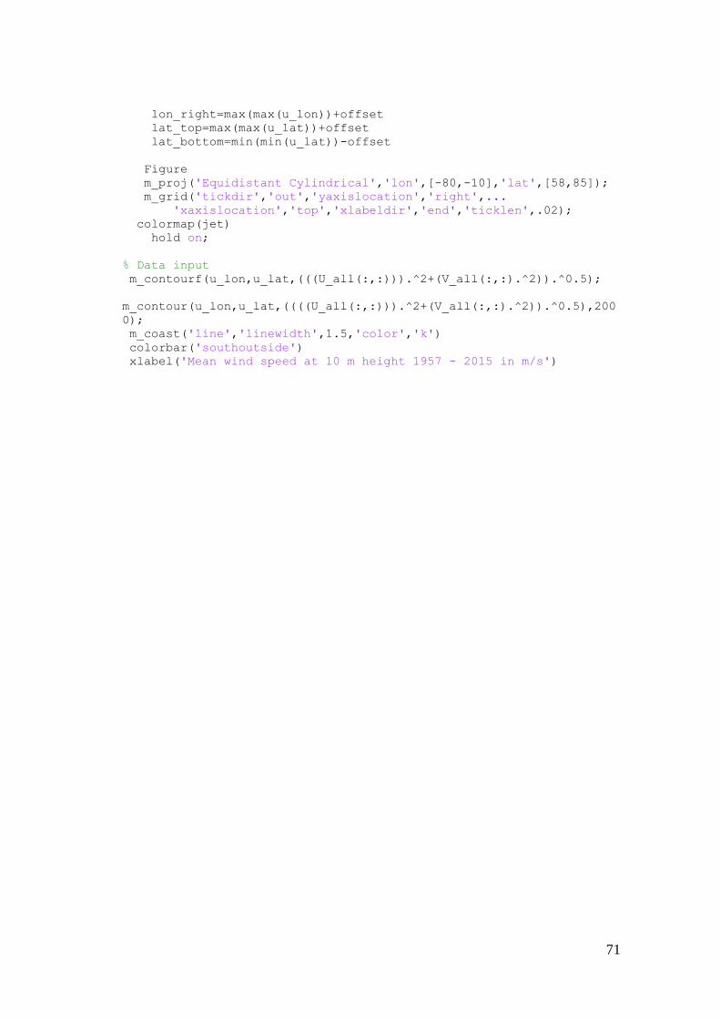
71
lon_right=max(max(u_lon))+offset lat_top=max(max(u_lat))+offset lat_bottom=min(min(u_lat))-offset
Figure m_proj('Equidistant Cylindrical','lon',[-80,-10],'lat',[58,85]); m_grid('tickdir','out','yaxislocation','right',... 'xaxislocation','top','xlabeldir','end','ticklen',.02); colormap(jet) hold on;
% Data input
m_contourf(u_lon,u_lat,(((U_all(:,:))).^2+(V_all(:,:).^2)).^0.5);
m_contour(u_lon,u_lat,((((U_all(:,:))).^2+(V_all(:,:).^2)).^0.5),200
0); m_coast('line','linewidth',1.5,'color','k') colorbar('southoutside') xlabel('Mean wind speed at 10 m height 1957 - 2015 in m/s')

72
APPENDIX 3 – Plotting (Geopotential example)
javaaddpath('C:\Users\josda921\Desktop\Matlab\netcdfAll-4.3.jar') addpath('C:\Users\josda921\Desktop\Matlab\mexcdf.r4053\mexcdf\snctoo
ls') addpath('C:\Users\josda921\Desktop\Matlab\mexcdf.r4053\mexcdf\mexnc'
) addpath('C:\Users\josda921\Desktop\Matlab\netcdf_toolbox\netcdf_tool
box') addpath ('C:\Program Files\MATLAB\R2015b\m_map1.4\m_map') g_lat= ncread('Mask_ZGRN11.nc','rlat'); g_lon = ncread('Mask_ZGRN11.nc','rlon'); LandSeaMask = ncread('Mask_ZGRN11.nc','LandSeaMask'); IceSheetMask= ncread('Mask_ZGRN11.nc','IceSheetMask'); geopotential = ncread('Mask_ZGRN11.nc','Geopotential'); g = 9.81665; Elevation=geopotential./g; fid=fopen(['C:\Program Files\MATLAB\R2015b\m_map1.4\m_map']) offset=0.5 lon_left=min(min(g_lon))-offset lon_right=max(max(g_lon))+offset lat_top=max(max(g_lat))+offset lat_bottom=min(min(g_lat))-offset % % height = uh % time = ut Figure % m_proj('Equidistant Cylindrical','lon',[lon_left
lon_right],'lat',[lat_bottom lat_top]); m_proj('Equidistant Cylindrical','lon',[-80,-10],'lat',[58,85]); m_grid('tickdir','out','yaxislocation','right',... 'xaxislocation','top','xlabeldir','end','ticklen',.02); colormap (jet) hold on m_contourf(g_lon,g_lat,((geopotential(:,:)))); m_contour(g_lon,g_lat,((geopotential(:,:))),1000); m_coast('line','linewidth',1.5,'color','k') colorbar('southoutside') xlabel('Geopotential')

73
APPENDIX 4 – Vestas V90 3MW Power curve and technical specifications
Figure 38 – Vestas V90 3MW power curve, Source: Vestas, 2016
Table 9 – Vestas V90 3MW, Technical Specifications, Source: Vestas, 2016

74
APPENDIX 5 – Combination Maps Script (ffgmax example)
fid=fopen(['C:\Program Files\MATLAB\R2015b\m_map1.4\m_map']) offset=0,5 % recommendation from tutorial m_map lon_left=min(min(ffgmax_lon1958))-offset lon_right=max(max(ffgmax_lon1958))+offset lat_top=max(max(ffgmax_lat1958))+offset lat_bottom=min(min(ffgmax_lat1958))-offset jet11=jet; Figure jet11=jet; for i=1:44 jet11(i,1:3)=1; end
colormap (jet11) hold on; m_contourf(ffgmax_lon1958,ffgmax_lat1958,((ffgmax_all(:,:)))); m_contour(ffgmax_lon1958,ffgmax_lat1958,((ffgmax_all(:,:))),2000);
m_proj('Equidistant Cylindrical','lon',[-80,-10],'lat',[58,85]); m_grid('tickdir','out','yaxislocation','right',... 'xaxislocation','top','xlabeldir','end','ticklen',.02); m_coast('line','linewidth',1.5,'color','k') colorbar('southoutside'); caxis ([1,20]) xlabel({'Average of Maximum wind speed at 10m height b) ','over
Greenland 1957 - 2015 in m/s'})

75
APPENDIX 6 – Multi-level data sorting (Site suggestion 4 example)
clear all clc % Insert netcdf toolbox javaaddpath('C:\Users\josda921\Desktop\Matlab\netcdfAll-4.3.jar') addpath('C:\Users\josda921\Desktop\Matlab\mexcdf.r4053\mexcdf\snctoo
ls') addpath('C:\Users\josda921\Desktop\Matlab\mexcdf.r4053\mexcdf\mexnc'
) addpath('C:\Users\josda921\Desktop\Matlab\netcdf_toolbox\netcdf_tool
box') % All years II=[1957 1958 1959 1960 1961 1962 1963 1964
1965 1966 1967 1968 1969 1970 1971 1972 1973
1974 1975 1976 1977 1978 1979 1980 1981 1982
1983 1984 1985 1986 1987 1988 1989 1990 1991
1992 1993 1994 1995 1996 1997 1998 1999 2000
2001 2002 2003 2004 2005 2006 2007 2008 2009
2010 2011 2012 2013 2014 2015] for l=1:length(II) m=II(l); % get wind speed, levels and date filename=sprintf('S4_%.4i.nc', m); level = ncread(filename,'level'); UU = ncread (filename,'uu'); VV = ncread (filename,'vv'); FF = ncread (filename,'ff'); date = ncread (filename,'dtg'); direction = ncread(filename,'dir'); U = ((UU.^2+VV.^2).^0.5); u = U.'; DIR = direction.'; % get organized date (years,months,day,hours) time_steps= length (date); year = date/1000000; month = (date -year*1000000)/10000; day = (date-year*1000000-month*10000)/100; hours = (date-year*1000000-month*10000-day*100); for i = 1:length(level); j=1:time_steps; um=u(j,i); ws = um; eval(['ws' num2str(level(i)) '=ws;']); for i = 1:length(level); j=1:time_steps; d=DIR(j,i); wd = d; eval(['wd' num2str(level(i)) '=wd;']); end end % Table 10 m S4_T10 = {'year';'month';'day';'hours';'ws10';'wd10'}.'; S4_Table10 =
table(year,month,day,hours,ws10,wd10,'VariableNames',S4_T10); eval(['S4_Table10' num2str(II(l)) '=S4_Table10;']);
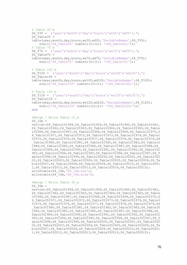
76
% Table 35 m S4_T35 = {'year';'month';'day';'hours';'ws35';'wd35'}.'; S4_Table35 =
table(year,month,day,hours,ws35,wd35,'VariableNames',S4_T35); eval(['S4_Table35' num2str(II(l)) '=S4_Table35;']); % Table 70 m S4_T70 = {'year';'month';'day';'hours';'ws70';'wd70'}.'; S4_Table70 =
table(year,month,day,hours,ws70,wd70,'VariableNames',S4_T70); eval(['S4_Table70' num2str(II(l)) '=S4_Table70;']);
% Table 100 m S4_T100 = {'year';'month';'day';'hours';'ws100';'wd100'}.'; S4_Table100 =
table(year,month,day,hours,ws100,wd100,'VariableNames',S4_T100); eval(['S4_Table100' num2str(II(l)) '=S4_Table100;']);
% Table 120 m S4_T120 = {'year';'month';'day';'hours';'ws120';'wd120'}.'; S4_Table120 =
table(year,month,day,hours,ws120,wd120,'VariableNames',S4_T120); eval(['S4_Table120' num2str(II(l)) '=S4_Table120;']); end
%Merge / Write Table 10_m S4_10m =
vertcat(S4_Table101958,S4_Table101959,S4_Table101960,S4_Table101961,
S4_Table101962,S4_Table101963,S4_Table101964,S4_Table101965,S4_Table
101966,S4_Table101967,S4_Table101968,S4_Table101969,S4_Table101970,S
4_Table101971,S4_Table101972,S4_Table101973,S4_Table101974,S4_Table1
01975,S4_Table101976,S4_Table101977,S4_Table101978,S4_Table101979,S4
_Table101980,S4_Table101981,S4_Table101982,S4_Table101983,S4_Table10
1984,S4_Table101985,S4_Table101986,S4_Table101987,S4_Table101988,S4_
Table101989,S4_Table101990,S4_Table101991,S4_Table101992,S4_Table101
993,S4_Table101994,S4_Table101995,S4_Table101996,S4_Table101997,S4_T
able101998,S4_Table101999,S4_Table102000,S4_Table102001,S4_Table1020
02,S4_Table102003,S4_Table102004,S4_Table102005,S4_Table102006,S4_Ta
ble102007,S4_Table102008,S4_Table102009,S4_Table102010,S4_Table10201
1,S4_Table102012,S4_Table102013,S4_Table102014,S4_Table102015); writetable(S4_10m,'S4_10m.txt'); writetable(S4_10m,'S4_10m.xlsx');
%Merge / Write Table 35_m S4_35m =
vertcat(S4_Table351958,S4_Table351959,S4_Table351960,S4_Table351961,
S4_Table351962,S4_Table351963,S4_Table351964,S4_Table351965,S4_Table
351966,S4_Table351967,S4_Table351968,S4_Table351969,S4_Table351970,S
4_Table351971,S4_Table351972,S4_Table351973,S4_Table351974,S4_Table3
51975,S4_Table351976,S4_Table351977,S4_Table351978,S4_Table351979,S4
_Table351980,S4_Table351981,S4_Table351982,S4_Table351983,S4_Table35
1984,S4_Table351985,S4_Table351986,S4_Table351987,S4_Table351988,S4_
Table351989,S4_Table351990,S4_Table351991,S4_Table351992,S4_Table351
993,S4_Table351994,S4_Table351995,S4_Table351996,S4_Table351997,S4_T
able351998,S4_Table351999,S4_Table352000,S4_Table352001,S4_Table3520
02,S4_Table352003,S4_Table352004,S4_Table352005,S4_Table352006,S4_Ta
ble352007,S4_Table352008,S4_Table352009,S4_Table352010,S4_Table35201
1,S4_Table352012,S4_Table352013,S4_Table352014,S4_Table352015);

77
writetable(S4_35m,'S4_35m.txt'); writetable(S4_35m,'S4_35m.xlsx'); clear S4_Table35*
%Merge /Write Table 70_m S4_70m =
vertcat(S4_Table701958,S4_Table701959,S4_Table701960,S4_Table701961,
S4_Table701962,S4_Table701963,S4_Table701964,S4_Table701965,S4_Table
701966,S4_Table701967,S4_Table701968,S4_Table701969,S4_Table701970,S
4_Table701971,S4_Table701972,S4_Table701973,S4_Table701974,S4_Table7
01975,S4_Table701976,S4_Table701977,S4_Table701978,S4_Table701979,S4
_Table701980,S4_Table701981,S4_Table701982,S4_Table701983,S4_Table70
1984,S4_Table701985,S4_Table701986,S4_Table701987,S4_Table701988,S4_
Table701989,S4_Table701990,S4_Table701991,S4_Table701992,S4_Table701
993,S4_Table701994,S4_Table701995,S4_Table701996,S4_Table701997,S4_T
able701998,S4_Table701999,S4_Table702000,S4_Table702001,S4_Table7020
02,S4_Table702003,S4_Table702004,S4_Table702005,S4_Table702006,S4_Ta
ble702007,S4_Table702008,S4_Table702009,S4_Table702010,S4_Table70201
1,S4_Table702012,S4_Table702013,S4_Table702014,S4_Table702015); writetable(S4_70m,'S4_70m.txt'); writetable(S4_70m,'S4_70.xlsx'); clear S4_Table70*
% Merge /Write Table 100_m S4_100m =
vertcat(S4_Table1001958,S4_Table1001959,S4_Table1001960,S4_Table1001
961,S4_Table1001962,S4_Table1001963,S4_Table1001964,S4_Table1001965,
S4_Table1001966,S4_Table1001967,S4_Table1001968,S4_Table1001969,S4_T
able1001970,S4_Table1001971,S4_Table1001972,S4_Table1001973,S4_Table
1001974,S4_Table1001975,S4_Table1001976,S4_Table1001977,S4_Table1001
978,S4_Table1001979,S4_Table1001980,S4_Table1001981,S4_Table1001982,
S4_Table1001983,S4_Table1001984,S4_Table1001985,S4_Table1001986,S4_T
able1001987,S4_Table1001988,S4_Table1001989,S4_Table1001990,S4_Table
1001991,S4_Table1001992,S4_Table1001993,S4_Table1001994,S4_Table1001
995,S4_Table1001996,S4_Table1001997,S4_Table1001998,S4_Table1001999,
S4_Table1002000,S4_Table1002001,S4_Table1002002,S4_Table1002003,S4_T
able1002004,S4_Table1002005,S4_Table1002006,S4_Table1002007,S4_Table
1002008,S4_Table1002009,S4_Table1002010,S4_Table1002011,S4_Table1002
012,S4_Table1002013,S4_Table1002014,S4_Table1002015); writetable(S4_100m,'S4_100m.txt'); writetable(S4_100m,'S4_100m.xlsx'); clear S4_Table10*
%Merge /Write Table 120_m S4_120m =
vertcat(S4_Table1201958,S4_Table1201959,S4_Table1201960,S4_Table1201
961,S4_Table1201962,S4_Table1201963,S4_Table1201964,S4_Table1201965,
S4_Table1201966,S4_Table1201967,S4_Table1201968,S4_Table1201969,S4_T
able1201970,S4_Table1201971,S4_Table1201972,S4_Table1201973,S4_Table
1201974,S4_Table1201975,S4_Table1201976,S4_Table1201977,S4_Table1201
978,S4_Table1201979,S4_Table1201980,S4_Table1201981,S4_Table1201982,
S4_Table1201983,S4_Table1201984,S4_Table1201985,S4_Table1201986,S4_T
able1201987,S4_Table1201988,S4_Table1201989,S4_Table1201990,S4_Table
1201991,S4_Table1201992,S4_Table1201993,S4_Table1201994,S4_Table1201
995,S4_Table1201996,S4_Table1201997,S4_Table1201998,S4_Table1201999,
S4_Table1202000,S4_Table1202001,S4_Table1202002,S4_Table1202003,S4_T
able1202004,S4_Table1202005,S4_Table1202006,S4_Table1202007,S4_Table

78
1202008,S4_Table1202009,S4_Table1202010,S4_Table1202011,S4_Table1202
012,S4_Table1202013,S4_Table1202014,S4_Table1202015); writetable(S4_120m,'S4_120m.txt'); writetable(S4_120m,'S4_120m.xlsx'); clear S4_Table120* S4_T*

79
APPENDIX 7 – Multi-level data sorting excel table [partial] (Site suggestion. 4
at 70 m example)
year month day hours ws70 wd70
1958 1 1 0 14,19357 -67,7196
1958 1 1 6 12,16852 -66,9924
1958 1 1 12 10,12886 -71,3956
1958 1 1 18 6,609215 -68,8102
1958 1 2 0 4,953244 -67,3313
1958 1 2 6 4,086501 -81,4205
1958 1 2 12 3,38676 -66,4936
1958 1 2 18 5,962494 -75,3552
1958 1 3 0 15,14227 -68,7911
1958 1 3 6 25,17072 -68,2775
1958 1 3 12 34,37239 -76,0236
1958 1 3 18 28,14148 -82,0715
1958 1 4 0 16,62599 -78,1093
1958 1 4 6 6,999499 206,0759
1958 1 4 12 13,33316 107,2921
1958 1 4 18 3,25301 191,7041
1958 1 5 0 7,166708 213,6116
1958 1 5 6 8,744693 214,4275
1958 1 5 12 10,23614 215,6163
1958 1 5 18 7,575628 209,5442
1958 1 6 0 9,952398 219,7833
1958 1 6 6 11,04434 225,4362
1958 1 6 12 7,862227 223,6972
1958 1 6 18 4,860005 -89,102
1958 1 7 0 13,42895 -71,7191
1958 1 7 6 8,602608 269,5666
1958 1 7 12 5,67432 228,0182
1958 1 7 18 0,818581 134,113
1958 1 8 0 3,492419 219,5161
1958 1 8 6 1,642628 108,6246
1958 1 8 12 2,489373 172,6976
1958 1 8 18 6,442151 246,426
1958 1 9 0 5,05945 216,6647
1958 1 9 6 3,420137 134,5707
1958 1 9 12 1,719642 114,5855
Table 10 – Multi-level data sorting excel table [partial] (Site s.. 4 at 70 m example)
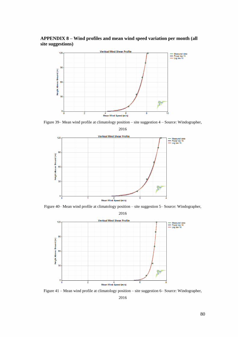
80
APPENDIX 8 – Wind profiles and mean wind speed variation per month (all
site suggestions)
Figure 39– Mean wind profile at climatology position – site suggestion 4 – Source: Windographer,
2016
Figure 40– Mean wind profile at climatology position – site suggestion 5– Source: Windographer,
2016
Figure 41 – Mean wind profile at climatology position – site suggestion 6– Source: Windographer,
2016

81
Figure 42 - Mean wind speed site suggestion 4 - monthly variation, Source: Windographer 2016
Figure 43 - Mean wind speed site suggestion 5 - monthly variation, Source: Windographer 2016
Figure 44 - Mean wind speed site suggestion 6 - monthly variation, Source: Windographer 2016

82
APPENDIX 9 – California – Annual Average Wind speed at 80 m and Redding
wind farms location
Figure 45 – California – Annual Average Wind speed at 80 m – Source: NREL 2010
Figure 46 – Wind Farms in the proximity of Redding (California) – Source: Google maps, 2016