Wilson Chpt 1

7/21/2019 Wilson Chpt 1

http://slidepdf.com/reader/full/wilson-chpt-1 1/24

Regression Analysis





Regression Analysis

Understanding and Building

Business and Economic Models

Using Excel

Second Edition

J. Holton Wilson, Barry P. Keating,and Mary Beal



Regression Analysis: Understanding and Building Business and Economic

Models Using Excel, Second Edition

Copyright © Business Expert Press, LLC, 2016.

All rights reserved. No part of this publication may be reproduced,

stored in a retrieval system, or transmitted in any form or by any

means—electronic, mechanical, photocopy, recording, or any other

except for brief quotations, not to exceed 400 words, without the prior

permission of the publisher.

First published in 2012 by

Business Expert Press, LLC

222 East 46th Street, New York, NY 10017

www.businessexpertpress.com

ISBN-13: 978-1-63157-385-9 (paperback)

ISBN-13: 978-1-63157-386-6 (e-book)

Business Expert Press Quantitative Approaches to Decision Making

Collection

Collection ISSN: 2163-9515 (print)

Collection ISSN: 2163-9582 (electronic)

Cover and interior design by Exeter Premedia Services Private Ltd.,

Chennai, India

First edition: 2012

Second edition: 2016

10 9 8 7 6 5 4 3 2 1

Printed in the United States of America.



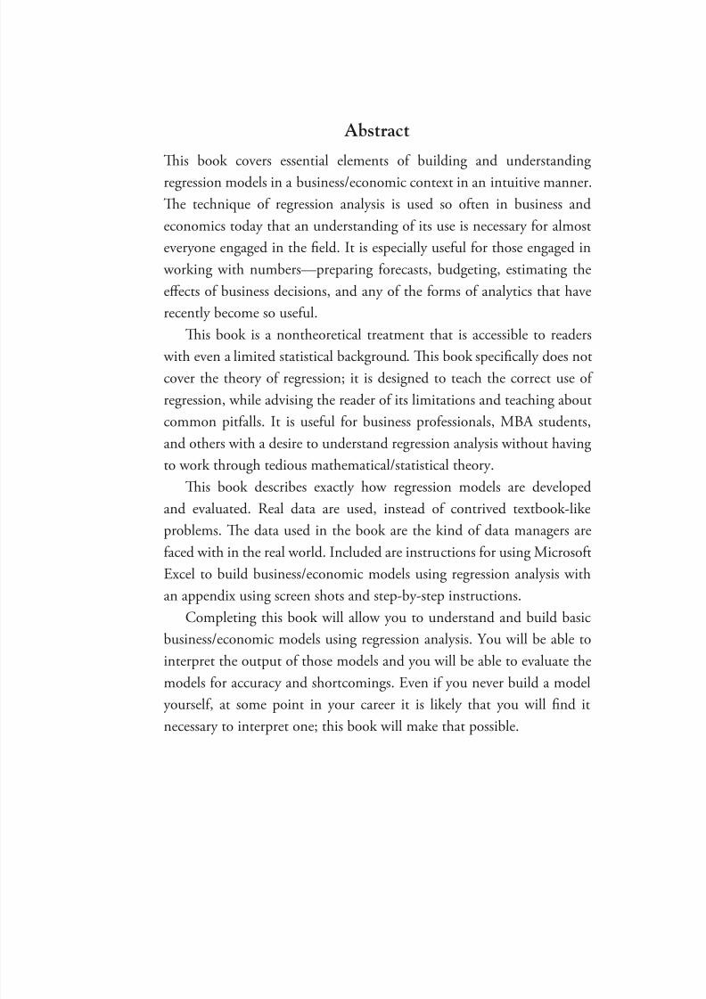
Abstract

Tis book covers essential elements of building and understanding

regression models in a business/economic context in an intuitive manner.

Te technique of regression analysis is used so often in business and

economics today that an understanding of its use is necessary for almost

everyone engaged in the field. It is especially useful for those engaged in

working with numbers—preparing forecasts, budgeting, estimating the

effects of business decisions, and any of the forms of analytics that have

recently become so useful.Tis book is a nontheoretical treatment that is accessible to readers

with even a limited statistical background. Tis book specifically does not

cover the theory of regression; it is designed to teach the correct use of

regression, while advising the reader of its limitations and teaching about

common pitfalls. It is useful for business professionals, MBA students,

and others with a desire to understand regression analysis without having

to work through tedious mathematical/statistical theory.Tis book describes exactly how regression models are developed

and evaluated. Real data are used, instead of contrived textbook-like

problems. Te data used in the book are the kind of data managers are

faced with in the real world. Included are instructions for using Microsoft

Excel to build business/economic models using regression analysis with

an appendix using screen shots and step-by-step instructions.

Completing this book will allow you to understand and build basicbusiness/economic models using regression analysis. You will be able to

interpret the output of those models and you will be able to evaluate the

models for accuracy and shortcomings. Even if you never build a model

yourself, at some point in your career it is likely that you will find it

necessary to interpret one; this book will make that possible.



vi ABSTRACT

Keywords

Regression analysis, ordinary least squares (OLS), time-series data,

cross-sectional data, dependent variables, independent variables, pointestimates, interval estimates, hypothesis testing, statistical significance,

confidence level, significance level, p-value, R-squared, coefficient of deter-

mination, multicollinearity, correlation, serial correlation, seasonality,

qualitative events, dummy variables, nonlinear regression models, market

share regression model, Abercrombie & Fitch Co.



Contents

Chapter 1 Background Issues for Regression Analysis ........................1

Chapter 2 Introduction to Regression Analysis ................................11

Chapter 3 Te Ordinary Least Squares (OLS)

Regression Model ...........................................................23

Chapter 4 Evaluation of Ordinary Least Squares(OLS) Regression Models ...............................................39

Chapter 5 Point and Interval Estimates From a

Regression Model ...........................................................65

Chapter 6 Multiple Linear Regression .............................................75

Chapter 7 A Market Share Multiple Regression Model ....................95

Chapter 8 Qualitative Events and Seasonality in

Multiple Regression Models ..........................................107

Chapter 9 Nonlinear Regression Models .......................................127

Chapter 10 Abercrombie & Fitch and Jewelry Sales

Regression Case Studies ................................................141

Chapter 11 Te Formal Ordinary Least Squares (OLS)

Regression Model .........................................................171

Appendix Some Statistical Background .........................................183

Index .................................................................................................189





CHAPTER 1

Background Issuesfor Regression Analysis

Chapter 1 Preview

When you have completed reading this chapter you will:

• Realize that this is a practical guide to regression not a

theoretical discussion.

• Know what is meant by cross-sectional data.

• Know what is meant by time-series data.

• Know to look for trend and seasonality in time-series data.

• Know about the three data sets that are used the most for

examples in the book.

• Know how to differentiate between nominal, ordinal, interval,

and ratio data.

• Know that you should use interval or ratio data when doing

regression.

• Know how to access the “Data Analysis” functionality in

Excel.

Introduction

Te importance of the use of regression models in modern business and

economic analysis can hardly be overstated. In this book, you will see

exactly how such models can be developed. When you have completed

the book you will understand how to construct, interpret, and evaluateregression models. You will be able to implement what you have learned

by using “Data Analysis” in Excel to build basic mathematical models of

business and economic relationships.





BACKGROUND ISSUES FOR REGRESSION ANALYSIS 3

Time-series Data

Time-series data are data that are collected over time for some particular

variable. For example, you might look at the level of unemployment by

year, by quarter, or by month. In this book, you will see examples that usetwo primary sets of time-series data. Tese are women’s clothing sales in

the United States and the occupancy for a hotel.

A graph of the women’s clothing sales is shown in Figure 1.2. When

you look at a time-series graph, you should try to see whether you observe

a trend (either up or down) in the series and whether there appears to

be a regular seasonal pattern to the data. Much of the data that we deal

with in business has either a trend or seasonality or both. Knowing thiscan be helpful in determining potential causal variables to consider when

building a regression model.

Te other time-series used frequently in the examples in this book is

shown in Figure 1.3. Tis series represents the number of rooms occu-

pied per month in a large independent motel. During the time period

being considered, there was a considerable expansion in the number

of casinos in the State, most of which had integrated lodging facilities.

As you can see in Figure 1.3, there is a downward trend in occupancy.

Te owners wanted to evaluate the causes for the decline. Tese data are

proprietary so the numbers are somewhat disguised as is the name of

the hotel. But the data represent real business data and a real business

problem.

Figure 1.1 The conference winning percentage for 82 basketball

teams: An example of cross-sectional data

Source: Statsheet at http://statsheet.com/mcb.

100.0%

80.0%

60.0%

40.0%

20.0%

0.0%

1 11 21 31 41 51 61 71 81



4 REGRESSION ANALYSIS

o help you understand regression analysis, these three sets of data will

be discussed repeatedly throughout the book. Also, in Chapter 10, you

will see complete examples of model building for quarterly Abercrombie

& Fitch sales and quarterly U.S. retail jewelry sales (both time-series

data). Tese examples will help you understand how to build regression

models and how to evaluate the results.

An Additional Data Issue

Not all data are appropriate for use in building regression models. Tis

means that before doing the statistical work of developing a regression

model you must first consider what types of data you have. One way

Figure 1.2 Women’s clothing sales per month in the United States in

millions of dollars: An example of time-series dataSource: www.economagic.com.

1 / 1 / 2 0 0 0

8 / 1 / 2 0 0 0

3 / 1 / 2 0 0 1

1 0 / 1 / 2 0 0 1

5 / 1 / 2 0 0 2

1 2 / 1 / 2 0 0 2

7 / 1 / 2 0 0 3

2 / 1 / 2 0 0 4

9 / 1 / 2 0 0 4

4 / 1 / 2 0 0 5

1 1 / 1 / 2 0 0 5

6 / 1 / 2 0 0 6

1 / 1 / 2 0 0 7

8 / 1 / 2 0 0 7

3 / 1 / 2 0 0 8

1 0 / 1 / 2 0 0 8

5 / 1 / 2 0 0 9

1 2 / 1 / 2 0 0 9

7 / 1 / 2 0 1 0

2 / 1 / 2 0 1 1

6,000

5,000

4,000

3,000

2,000

1,000

0

Figure 1.3 Stoke’s Lodge occupancy per month: A second example of

time-series data.

Source: Proprietary.

J a n - 0

0

J u l - 0 0

J a n - 0

1

J u l - 0 1

J a n - 0

2

J u l - 0 2

J u l - 0 3

J a n - 0

3

J u l - 0 4

J a n - 0

4

J u l - 0 5

J a n - 0

5

J u l - 0 6

J a n - 0

6

J u l - 0 7

J a n - 0

7

J a n - 0

8

14,000

12,000

10,000

8,000

6,000

4,000

2,000

0




data are often classified is to use a hierarchy of four data types. Tese

are: nominal, ordinal, interval, and ratio. In doing regression analysis,

the data that you use should be composed of either interval or ratio

numbers.1 A short description of each will help you recognize when you

have appropriate (interval or ratio) data for a regression model.

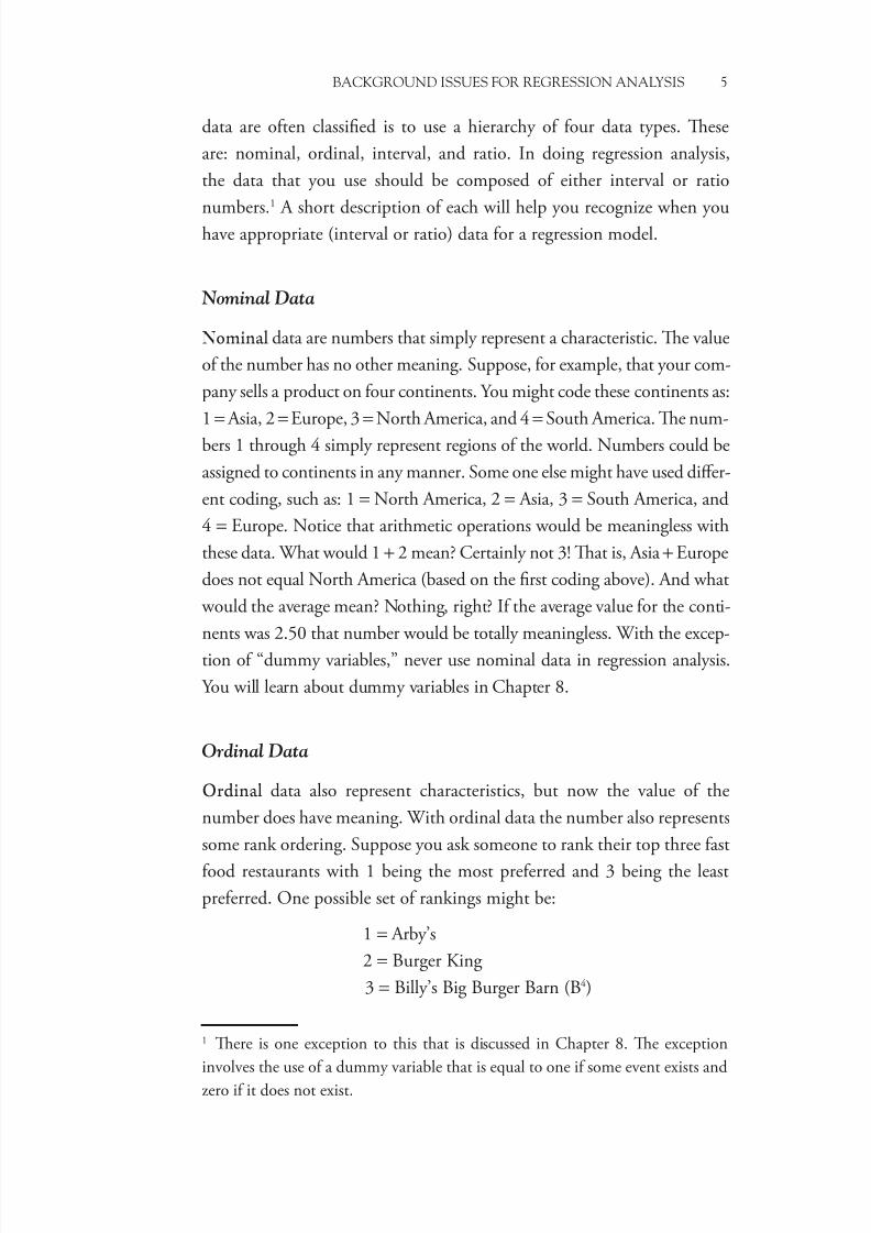
Nominal Data

Nominal data are numbers that simply represent a characteristic. Te value

of the number has no other meaning. Suppose, for example, that your com-

pany sells a product on four continents. You might code these continents as:

1 = Asia, 2 = Europe, 3 = North America, and 4 = South America. Te num-

bers 1 through 4 simply represent regions of the world. Numbers could be

assigned to continents in any manner. Some one else might have used differ-

ent coding, such as: 1 = North America, 2 = Asia, 3 = South America, and

4 = Europe. Notice that arithmetic operations would be meaningless with

these data. What would 1 + 2 mean? Certainly not 3! Tat is, Asia + Europe

does not equal North America (based on the first coding above). And what would the average mean? Nothing, right? If the average value for the conti-

nents was 2.50 that number would be totally meaningless. With the excep-

tion of “dummy variables,” never use nominal data in regression analysis.

You will learn about dummy variables in Chapter 8.

Ordinal Data

Ordinal data also represent characteristics, but now the value of the

number does have meaning. With ordinal data the number also represents

some rank ordering. Suppose you ask someone to rank their top three fast

food restaurants with 1 being the most preferred and 3 being the least

preferred. One possible set of rankings might be:

1 = Arby’s

2 = Burger King 3 = Billy’s Big Burger Barn (B4)

1 Tere is one exception to this that is discussed in Chapter 8. Te exception

involves the use of a dummy variable that is equal to one if some event exists and

zero if it does not exist.




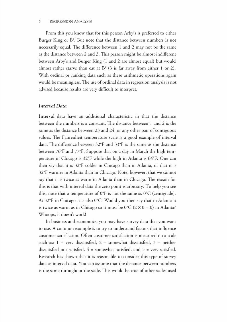
From this you know that for this person Arby’s is preferred to either

Burger King or B4. But note that the distance between numbers is not

necessarily equal. Te difference between 1 and 2 may not be the same

as the distance between 2 and 3. Tis person might be almost indifferent

between Arby’s and Burger King (1 and 2 are almost equal) but would

almost rather starve than eat at B4 (3 is far away from either 1 or 2).

With ordinal or ranking data such as these arithmetic operations again

would be meaningless. Te use of ordinal data in regression analysis is not

advised because results are very difficult to interpret.

Interval Data

Interval data have an additional characteristic in that the distance

between the numbers is a constant. Te distance between 1 and 2 is the

same as the distance between 23 and 24, or any other pair of contiguous

values. Te Fahrenheit temperature scale is a good example of interval

data. Te difference between 32°F and 33°F is the same as the distance

between 76°F and 77°F. Suppose that on a day in March the high tem-perature in Chicago is 32°F while the high in Atlanta is 64°F. One can

then say that it is 32°F colder in Chicago than in Atlanta, or that it is

32°F warmer in Atlanta than in Chicago. Note, however, that we cannot

say that it is twice as warm in Atlanta than in Chicago. Te reason for

this is that with interval data the zero point is arbitrary. o help you see

this, note that a temperature of 0°F is not the same as 0°C (centigrade).

At 32°F in Chicago it is also 0°C. Would you then say that in Atlanta itis twice as warm as in Chicago so it must be 0°C (2 × 0 = 0) in Atlanta?

Whoops, it doesn’t work!

In business and economics, you may have survey data that you want

to use. A common example is to try to understand factors that influence

customer satisfaction. Often customer satisfaction is measured on a scale

such as: 1 = very dissatisfied, 2 = somewhat dissatisfied, 3 = neither

dissatisfied nor satisfied, 4 = somewhat satisfied, and 5 = very satisfied.Research has shown that it is reasonable to consider this type of survey

data as interval data. You can assume that the distance between numbers

is the same throughout the scale. Tis would be true of other scales used




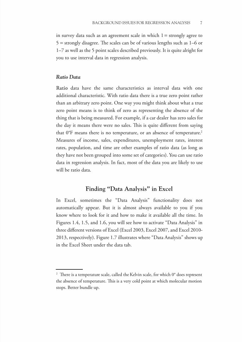
in survey data such as an agreement scale in which 1 = strongly agree to

5 = strongly disagree. Te scales can be of various lengths such as 1–6 or

1–7 as well as the 5 point scales described previously. It is quite alright for

you to use interval data in regression analysis.

Ratio Data

Ratio data have the same characteristics as interval data with one

additional characteristic. With ratio data there is a true zero point rather

than an arbitrary zero point. One way you might think about what a true

zero point means is to think of zero as representing the absence of the

thing that is being measured. For example, if a car dealer has zero sales for

the day it means there were no sales. Tis is quite different from saying

that 0°F means there is no temperature, or an absence of temperature.2

Measures of income, sales, expenditures, unemployment rates, interest

rates, population, and time are other examples of ratio data (as long as

they have not been grouped into some set of categories). You can use ratio

data in regression analysis. In fact, most of the data you are likely to use

will be ratio data.

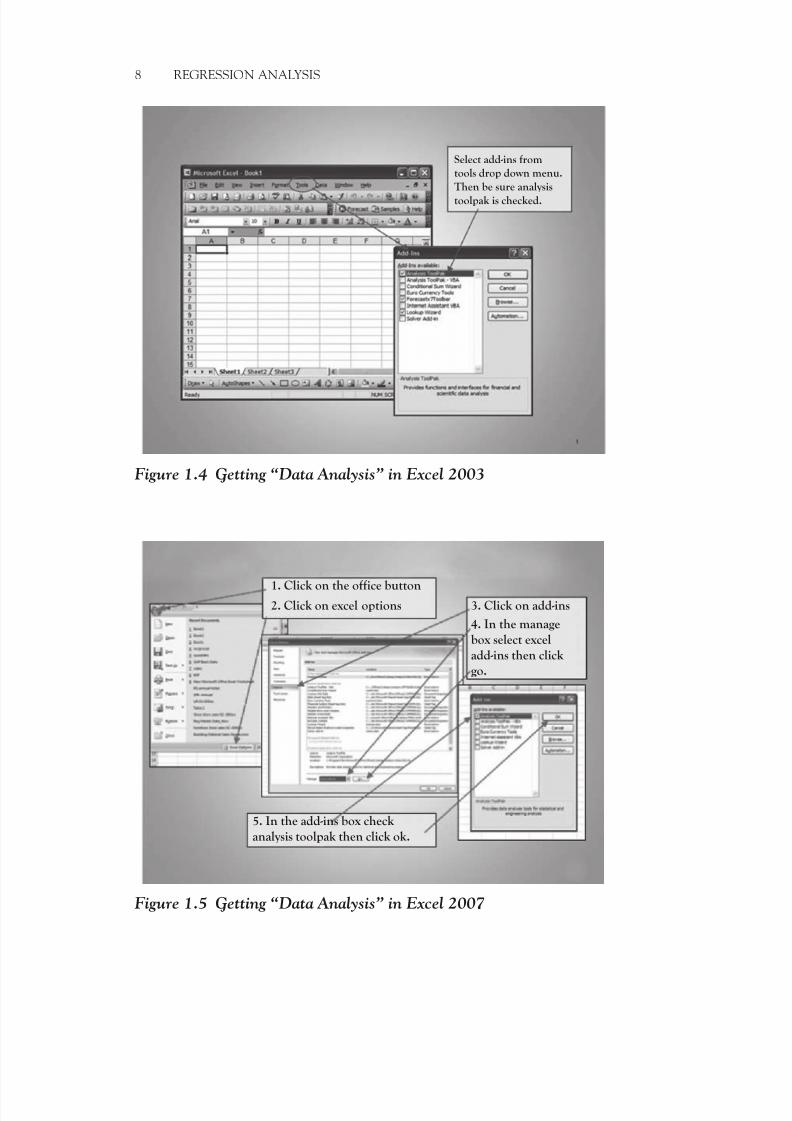
Finding “Data Analysis” in Excel

In Excel, sometimes the “Data Analysis” functionality does not

automatically appear. But it is almost always available to you if you

know where to look for it and how to make it available all the time. InFigures 1.4, 1.5, and 1.6, you will see how to activate “Data Analysis” in

three different versions of Excel (Excel 2003, Excel 2007, and Excel 2010-

2013, respectively). Figure 1.7 illustrates where “Data Analysis” shows up

in the Excel Sheet under the data tab.

2 Tere is a temperature scale, called the Kelvin scale, for which 0° does represent

the absence of temperature. Tis is a very cold point at which molecular motion

stops. Better bundle up.




Figure 1.4 Getting “Data Analysis” in Excel 2003

Select add-ins from

tools drop down menu.Then be sure analysis

toolpak is checked.

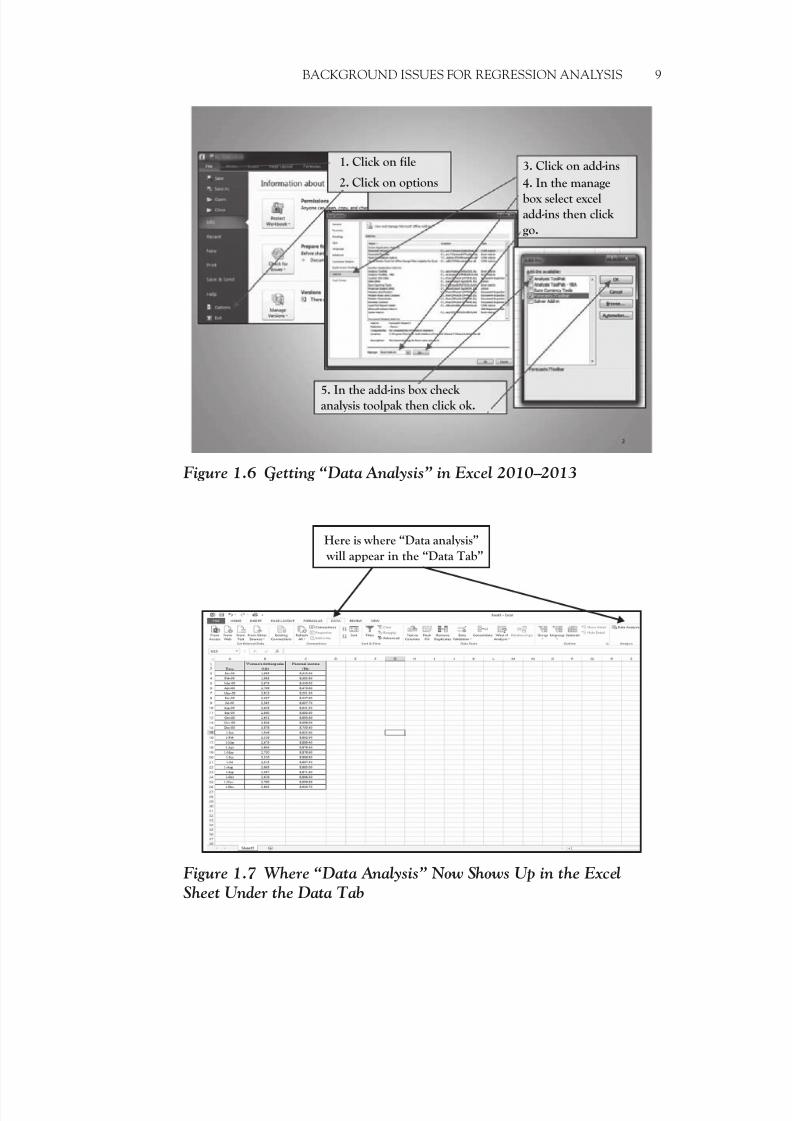
Figure 1.5 Getting “Data Analysis” in Excel 2007

1. Click on the office button

2. Click on excel options

5. In the add-ins box check

analysis toolpak then click ok.

3. Click on add-ins

4. In the manage

box select excel

add-ins then click

go.




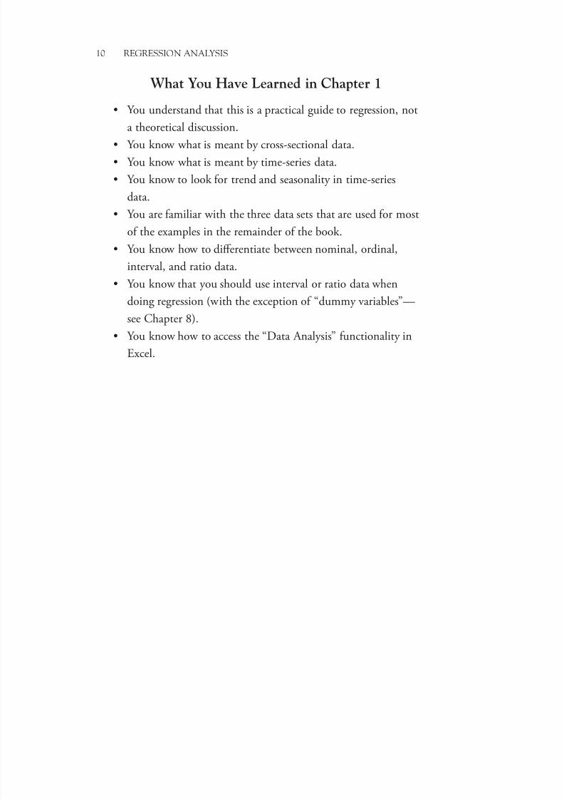
Figure 1.6 Getting “Data Analysis” in Excel 2010–2013

1. Click on file

2. Click on options

5. In the add-ins box check

analysis toolpak then click ok.

3. Click on add-ins

4. In the manage

box select excel

add-ins then click

go.

Figure 1.7 Where “Data Analysis” Now Shows Up in the ExcelSheet Under the Data Tab

Here is where “Data analysis”

will appear in the “Data Tab”




What You Have Learned in Chapter 1

• You understand that this is a practical guide to regression, not

a theoretical discussion.• You know what is meant by cross-sectional data.

• You know what is meant by time-series data.

• You know to look for trend and seasonality in time-series

data.

• You are familiar with the three data sets that are used for most

of the examples in the remainder of the book.

• You know how to differentiate between nominal, ordinal,interval, and ratio data.

• You know that you should use interval or ratio data when

doing regression (with the exception of “dummy variables”—

see Chapter 8).

• You know how to access the “Data Analysis” functionality in

Excel.



Index

Abercrombie & Fitch sales regressionmodel

five-step evaluation modeldummy variables (RUEHL, Gilly

Hicks), 153–157personal income, 145–147seasonal dummy variables,

150–153unemployment rate, 147–150

hypothesisdummy variables (RUEHL, Gilly

Hicks), 145personal income, 143–144seasonal dummy variables, 144unemployment rate, 144

Adjusted coefficient of determination,84–851

Adjusted R-square, 84–85 AIC. See Akaike information criterion Akaike information criterion (AIC),

177 Analysis of variance (ANOVA), 86,

187 Annual values for women’s clothing

sales (AWCS), 28–29, 62–63 ANOVA. See Analysis of variance

Approximate 95% confidence intervalestimatecollege basketball winning

percentage, 72–73concept of, 66–68market share multiple regression

model, 103multiple linear regression, 89

women’s clothing sales (WCS),70–72

Bivariate linear regression (BLR)model, 24

Business applications, regressionanalysis

cross-sectional data, 2–3time-series data, 3–4

Central tendency mean, 184median, 185mode, 185

Cobb-Douglas production function,136–137

Coefficient of determinationadjusted, 84–85definition of, 50development of, 174–176

College basketball winning percentageactual vs. predicted values, 20approximate 95% confidence

interval estimate, 72–73cross-sectional data, 18, 19point estimate, 69scatterplot, 19

Computed test statistic, 46, 49, 55,81, 86

Confidence interval, 66–68Constant. See InterceptCorrelation matrix

independent variables, 124

Miller’s Foods’ market shareregression, 103

multicollinearity, 124personal income, 153, 156RUEHL and Gilly Hicks, 156seasonal dummy variables, 153, 156unemployment rate, 153, 156

Critical valuesDurbin-Watson statistic, 60–61F-distribution at 95% confidence

level, 92–93F-test, 86hypothesis test, 45

Cross-sectional data, 2–3Cubic functions, 130–134



190 INDEX

Data Analysisdata tab, 9in Excel 2003, 8

in Excel 2007, 8in Excel 2010–2013, 9OLS regression model in Excel,

32–37Data types

interval data, 6–7nominal data, 5ordinal data, 5–6ratio data, 7

Degrees of freedom, 58

Dependent variable, 24Dispersion

range, 186standard deviation, 186standard error, 187variance, 186–187

Dummy variables Abercrombie & Fitch sales

regression modelfive-step evaluation model,

153–157hypothesis, 145

definition of, 108hypotheses, 120–121multiple linear regression, 108–111seasonality, 111–117uses of, 108

women’s clothing sales, 111–117Durbin-Watson (DW) statistic, 102

calculation in Excel, 62–64

critical values, 60–61evaluation, 53

Explained variation, 175Explanatory power of model

Abercrombie & Fitch salesdummy variables, 155–156personal income, 147seasonal dummy variables, 152

unemployment rate, 163market share multiple regressionmodel, 101–102

multiple linear regression, 84–87ordinary least squares (OLS)

regression model, 50Stoke’s Lodge occupancy, 55–56

Formal OLS regression modelalternative models, 179–181mathematical approach of,

171–174R-square development, 174–176scattergram of Miller’s foods’

market share, 177–179software programs

Akaike information criterion,177

Schwarz criterion, 177F-statistic, 86

Gilly Hicks, dummy variable Abercrombie & Fitch sales,

153–157correlation matrix, 156hypothesis, 145

Homoscedasticity, 31Hypothesis test, 43–50

Independent variable, 24

Interceptbasketball winning percentage,

26–27definition of, 24–25

women’s clothing sales model,25–26

Interval data, 6–7

Market share multiple regression

modelapproximate 95% confidenceinterval estimate, 103

explanatory power of model,101–102

model does make sense?, 98–99multicollinearity, 102–103point estimate, 103–104serial correlation, 102statistical significance, 99–101

three-dimensional visualrepresentation, 103–104Mean, 184Median, 185Miller’s Foods’ market share. See

also Market share multipleregression model



INDEX 191

alternative models, 177building and evaluating,

179–181

scattergramadvertising, 179index of competitor’s advertising,

178price, 178

Mode, 185 MONEYBALL, 18, 73Monthly room occupancy (MRO)

actual and predicted values for,119–120

function of gas price, 119multiple linear regression, 77, 78OLS regression models, 54Stoke’s Lodge, 118

MRO. See Monthly room occupancy Multicollinearity

Abercrombie & Fitch salesdummy variables, 156personal income, 147seasonal dummy variables, 153

unemployment rate, 150correlation matrix, 124market share multiple regression

model, 102–103multiple linear regression, 87–89

Multiple linear regressionapproximate 95% confidence

interval, 89dummy variables, 108–111general form of, 76point and interval estimate, 89–90Stoke’s Lodge model

actual vs. predicted regressionestimates, 90

explanatory power of the model,84–87

model does make sense?, 78–80monthly room occupancy, 78multicollinearity, 87–89

serial correlation, 87statistical significance, 80–84Multiplicative functions, 136–139

Nominal data, 5Nonlinear regression models

cubic functions, 130–134multiplicative functions, 136–139quadratic functions, 128–131

reciprocal functions, 134–136

Ordinal data, 5–6Ordinary least squares (OLS)

regression modelannual values for women’s clothing

sales, 28–29criterion for, 27–28data analysis in Excel, 32–37evaluation process

explanatory power of model, 50model does make sense?, 40–41serial correlation, 50–53statistical significance, 41–50

formalalternative models, 179–181mathematical approach of,

171–174R-square development, 174–176scattergram of Miller’s foods’

market share, 177–179mathematical assumptions

dispersion, 31normal distribution, 31–32probability distribution, 30–31

Stoke’s Lodge occupancy explanatory power of, 55–56model makes sense?, 54–55serial correlation, 55statistical significance, 56

theory vs. practice, 32Over specification of regression

model. See multicollinearity

Personal income (PI) Abercrombie & Fitch sales,

143–144correlation matrix, 153, 156scattergram, 14–16

Point estimate

college basketball winningpercentage, 69

definition of, 66illustration of, 66market share multiple regression

model, 103–104



192 INDEX

multiple linear regression, 89–90 women’s clothing sales, 68

Population, 183–184

Population parameter, 184Power function. See Multiplicativefunctions

Probability distributionordinary least squares (OLS)

regression model, 30–31p-value, 82–84

Quadratic functions, 128–131

Range, 186Ratio data, 7Reciprocal functions, 134–136Regression analysis

Abercrombie & Fitch salesregression model

dummy variables (RUEHL, GillyHicks), 145, 153–157

personal income, 143–147seasonal dummy variables, 144,

150–153unemployment rate, 144,

147–150in business applications

cross-sectional data, 2–3time-series data, 3–4

college basketball winningpercentage

actual vs. predicted values, 20

cross-sectional data, 18, 19scatterplot, 19data types

interval data, 6–7nominal data, 5ordinal data, 5–6ratio data, 7

description of, 11nonlinear regression models

cubic functions, 130–134

multiplicative functions,136–139quadratic functions, 128–131reciprocal functions, 134–136

predicted warnings, 20–21

women’s clothing salesactual vs. predicted results,

16–17vs.

personal income, 14–16scattergram, 14–16time-series data, 14

R-Square. See Coefficient ofdetermination

RUEHL, dummy variable Abercrombie & Fitch sales,

153–157correlation matrix, 156hypothesis, 145

Sample, 183–184SC. See Schwarz criterionScattergram

cubic functions, 128–132Miller’s foods’ market share

advertising, 179index of competitor’s advertising,

178price, 178

OLS regression models, 42, 43reciprocal functions, 135

women’s clothing sales, 14–16Schwarz criterion (SC), 177Seasonal dummy variables

Abercrombie & Fitch salesregression model

explanatory power of model, 152hypothesis, 144

multicollinearity, 153serial correlation, 152–153statistical significance, 152

correlation matrix, 153, 156 womens’ clothing sales (WCS)

complete regression results, 114monthly basis, 111, 112multiple regression model,

112–113regression analyses, 115

regression coefficients, 114–115UMICS and WUR, 115–117Second reciprocal function, 136SEE. See Standard error of the

estimate



INDEX 193

Serial correlation Abercrombie & Fitch sales

dummy variables, 156

personal income, 147seasonal dummy variables,152–153

unemployment rate, 150causes of, 52market share multiple regression

model, 102multiple linear regression, 87ordinary least squares (OLS)

regression model, 50–53

Stoke’s Lodge model, 56Simple linear regression marker share

model, 96–97Slope

basketball winning percentage,26–27

definition of, 25 women’s clothing sales model,

25–26Software programs

Akaike information criterion, 177Schwarz criterion, 177

SSR. See Sum of squared regressionStandard deviation, 186Standard error, 187Standard error of the estimate (SEE),

66–67approximate 95 percent confidence

interval, 66–67Excel’s regression output, 69–70

market share model, 103Statistical significance

Abercrombie & Fitch salesdummy variables, 154–155personal income, 145seasonal dummy variables, 152unemployment rate, 148

market share multiple regressionmodel, 99–101

multiple linear regression, 80–84ordinary least squares (OLS)

regression model, 41–50Stoke’s Lodge occupancy, 55

Stoke’s Lodge occupancy monthly room occupancy, 118

multiple linear regressionactual vs. predicted regression

estimates, 90

explanatory power of the model,84–87model does make sense?, 78–80monthly room occupancy, 78multicollinearity, 87–89serial correlation, 87statistical significance, 80–84

ordinary least squares (OLS)regression model

explanatory power of, 55–56

model makes sense?, 54–55serial correlation, 56statistical significance, 55

regression results, 123Sum of squared regression (SSR), 86

t-distribution, 59Time-series data, 3–4Total variation, 175t-ratio, 46, 49, 55

t-test, 42, 45, 46. See also hypothesistest

UMICS. See University of MichiganIndex of Consumer Sentiment

Unemployment rate, 144, 147–150,153, 156, 163

Unexplained variation, 175University of Michigan Index

of Consumer Sentiment(UMICS), 115–116

Variance, 186–187

Women’s clothing sales (WCS)actual vs. predicted results, 16–17annual values for OLS model,

28–29approximate 95% confidence

interval estimate, 70–72dummy variables

complete regression results, 114monthly basis, 111, 112multiple regression model, 112–113



194 INDEX

regression analyses, 115regression coefficients, 114–115UMICS and WUR, 115–117

intercept for, 25–26partial regression statistics, 72vs. personal income, 14–16

point estimate, 68scattergram, 14–16slope for, 25–26

time-series data, 14 Women’s unemployment rate (WUR),116, 117

Documents

Wilson Chpt 1