Draft version December 13, 2017Typeset using LATEX twocolumn style in AASTeX61

CHEMICALLY-DISSECTED ROTATION CURVES OF THE GALACTIC BULGE FROM MAIN SEQUENCE

PROPER MOTIONS∗

William I. Clarkson,1 Annalisa Calamida,2 Kailash C. Sahu,2 Thomas M. Brown,2 Mario Gennaro,2

Roberto Avila,2 Jeff Valenti,2 Victor P. Debattista,3 R. Michael Rich,4 Dante Minniti,5, 6, 7 andManuela Zoccali7, 8

1Department of Natural Sciences, University of Michigan-Dearborn, 4901 Evergreen Rd. Dearborn, MI, 48128, USA2Space Telescope Science Institute, 3700 San Martin Drive, Baltimore, MD 21218, USA3Jeremiah Horrocks Institute, University of Central Lancashire, Preston PR1 2HE, UK4Division of Astronomy & Astrophysics, University of California, Los Angeles, 430 Portola Plaza, Box 951547, Los Angeles, CA

90095-1547, USA5Departamento de Ciencias Fısicas, Facultad de Ciencias Exactas, Universidad Andres Bello, Av. Fernandez Concha 700, Las Condes,

Santiago, Chile6Vatican Observatory, V00120 Vatican City State, Italy7Millennium Institute of Astrophysics, Av. Vicuna Mackenna 4860, 782-0436 Macul, Santiago, Chile8Instituto de Astrofısica, Pontificia Universidad Catolica de Chile, Av. Vicuna Mackenna 4860, Santiago, Chile

ABSTRACT

We report results from an exploratory study implementing a new probe of Galactic evolution using archival Hubble

Space Telescope imaging observations. Precise proper motions are combined with photometric relative metallicity and

temperature indices, to produce the proper motion rotation curves of the Galactic bulge separately for metal-poor

and metal-rich Main Sequence samples. This provides a “pencil-beam” complement to large-scale wide-field surveys,

which to-date have focused on the more traditional bright Giant Branch tracers and which, taken together, remain

somewhat agnostic on the existence of any difference in mean rotation between metal-poor and metal-rich components

within the Galactic bulge, particularly within a few degrees of the Galactic mid-plane.

We find strong evidence that the Galactic bulge rotation curves drawn from “metal-rich” and “metal-poor” samples

are indeed discrepant. The “metal-rich” sample shows greater rotation amplitude and a steeper gradient against line

of sight distance, as possibly a stronger central concentration along the line of sight. We also investigate selection

effects this would imply for the longitudinal proper motion cut often used to isolate a “pure-bulge” sample. Extensive

investigation of synthetic stellar populations suggest that instrumental and observational artefacts are unlikely to

account for the observed rotation curve differences.

Thus, proper motion-based rotation curves can be used to probe chemo-dynamical correlations for Main Sequence

tracer stars, which are orders of magnitude more numerous in the Galactic Bulge than the bright Giant Branch tracers.

We discuss briefly the prospect of using this new tool to constrain detailed models of Galactic formation and evolution.

Keywords: Galaxy: bulge, Galaxy: disk, Galaxy: kinematics and dynamics, instrumentation: high

angular resolution, methods: data analysis, techniques: photometric

Corresponding author: Will Clarkson

wiclarks@umich.edu

∗ Based on observations made with the NASA/ESA Hubble Space Telescope and obtained from the data archive at the Space TelescopeScience Institute. STScI is operated by the Association of Universities for Research in Astronomy, Inc. under NASA contract NAS 5-26555.

2 Clarkson, Calamida, Sahu, Brown, Gennaro, Avila, Valenti, et al.

1. INTRODUCTION

The diversity of observed properties of the Galactic

bulge has challenged attempts to provide a coherent

explanation for its formation and subsequent develop-

ment. For example, while color-magnitude diagrams

suggest the majority of bulge stars are likely older than

∼ 8 Gy (e.g. Zoccali et al. 2003, Kuijken & Rich 2002,

Clarkson et al. 2008, Calamida et al. 2014, although

see, e.g. Nataf & Gould 2012, Haywood et al. 2016

and Bensby et al. 2017 for alternative interpretation),

minority populations of younger objects have been de-

tected (e.g. Sevenster et al. 1997, van Loon et al. 2003).

That measurements of even bulk parameters like bar

orientation and axis ratio have not converged with time

(e.g. Vanhollebeke et al. 2009) is consistent with a de-

pendence of these properties on the ages of the tracers

used. For example, Catchpole et al. (2016) find distinct

bar/bulge spatial structures coexisting in the same vol-

ume, traced by Mira populations of different ages. As

shown by Ness et al. (2013a), the various apparent ob-

servational contradictions can be resolved by a scenario

in which most bulge stars did indeed form early but later

were rearranged into their present-day spatial and kine-

matic distributions by disk-driven evolution. Recent re-

views of Galactic bulge observations and formation sce-

narios include Rich (2015), Babusiaux (2016), Zoccali &

Valenti (2016) and Nataf (2017).

Observations have long suggested a co-dependence be-

tween chemical abundance and kinematics in the bulge,

particularly as traced by velocity dispersion, providing

an observational test of formation and evolution scenar-

ios (e.g. Rich 1990; Minniti 1996). Metal-rich samples

show a steeper increase in radial velocity dispersion with

Galactic latitude than do the metal-poor objects (whose

dispersion-latitude profile is only gently sloped and may

be flat); while differences exist in the literature as to

the [Fe/H] cuts used to define the two samples, by lat-

itude |b| . 3◦ the metal-poor and metal-rich samples

have consistent radial velicity dispersions (Figure 4 of

Babusiaux 2016 presents a recent compilation for fields

along the Bulge minor axis). For the very inner-most

fields in the Bulge (|b| . 1.0◦ and |l| . 2◦), a radial

velocity dispersion “inversion” may even be present (an

expression of a steeper dispersion gradient with longi-

tude for metal-rich objects), with the metal-rich stars

showing greater velocity dispersion than the metal-poor

objects in bins closest to the Galactic center (e.g. Babu-

siaux et al. 2014; Zoccali et al. 2017). In a complemen-

tary manner, Spaenhauer et al. (1992) traced the proper

motion dispersion for a sample of 57 Bulge giants to-

wards Baade’s window, allowing the first test of Bulge

chemical and kinematic co-dependence using proper mo-

tions. No statistically significant discrepancy in proper

motion dispersion was found between metal-poor (de-

fined as [Fe/H] < 0.0) and metal-rich ([Fe/H] > 0.0)

objects (with Galactic latitudinal proper motion disper-

sion difference ∆σµ,l ≈ 0.5± 0.6 mas yr−1 between the

samples), although the sample size was not large.

The implications of observational chemical-dynamical

correlations for formation models of the inner Milky

Way are the subject of vigorous ongoing observational

and theoretical research. For example, Debattista et al.

(2017) showed that samples drawn from a continuous

metallicity distribution in a pure-disk galaxy model can

be “kinematically fractionated” by bar formation into

metal-rich and metal-poor populations with quite dif-

ferent morphology and dynamics, depending on their

initial (Galactocentric) radial velocity dispersions. This

is consistent with the tendency of the stellar population

in the “X”-shape to be dominated by metal-rich stars

(Vasquez et al. 2013), as has now also been observed

in NGC 4710, a nearby disk-dominated galaxy viewed

almost edge-on (Gonzalez et al. 2016, 2017).

Indeed, Shen et al. (2010) argue that the radial veloc-

ities and morphology of Bulge stellar populations show

no need for a substantial spheroidal “Classical” bulge

component (at the level of . 8% of the disk mass), ar-

guing that the Milky Way can be characterized as a

pure-disk galaxy. Nonetheless, a small spheroidal com-

ponent probably has been detected, although its likely

contribution to the total Bulge mass is likely well under

10% (Kunder et al. 2016). Interpretation of this compo-

nent in the context of Galactic formation is not clear; it

might, for example, represent part of the Halo popula-

tion that has also probably been detected in the inner

Milky Way (Koch et al. 2016).

1.1. Does bulge rotation depend on metallicity?

The trend in bulge mean radial velocity (against

Galactic longitude or Galactocentric radius) may also

vary with metallicity, but here the magnitude (or even

existence) of such a dependence is less clear than for the

velocity dispersions.1

Harding & Morrison (1993) and Minniti (1996)

demonstrated that “metal-rich” stars show a gradient

in circular speed with Galactocentric radius, consistent

with the “solid body”-type rotation traced by plan-

etary nebulae (Kinman et al. 1988), Miras (Menzies

1990) and SiO masers (Nakada et al. 1993). In con-

1 The interpretation of any radial velocity-metallicity bifurca-tion is somewhat complicated by variations both in calibrationof the [Fe/H] scale and in the definitions authors use to define“metal-rich” and “metal-poor” samples.

Bulge rotation curves from main-sequence proper motions 3

trast, metal-poor objects (then identified with the halo)

showed no strong evidence for a rotational trend. (Note

that Minniti 1996 defined “metal-rich” as objects with

[Fe/H] > −1.00, quite different from the boundary usu-

ally used in more recent studies.)

The large ARGOS survey of three-dimensional mo-

tions of (mostly clump) giants at |b| ≥ 4◦ showed no

[Fe/H] -dependence of the mean radial velocity trend

with Galactic longitude, for sub-samples of objects with

[Fe/H] > −1.0; the objects in this range show cylin-

drical rotation, with the sub-component at [Fe/H] &−0.5 showing separate kinematic identity; Ness et al.

2013b). Among the ARGOS sample, the metal-poor

objects at [Fe/H] . −1.0 do show a slightly lower am-

plitude of rotation curve (with the large-longitude veloc-

ity plateau at ∼ ±50 km s−1 compared to ∼ ±100 km

s−1 or more for [Fe/H] > −1.0).

Then Kunder et al. (2016) found that their metal-

poor RR Lyrae sample with mostly sub-solar metallici-

ties (−2.4 < [Fe/H] . +0.3, peaking at [Fe/H] ∼ −1.0)

shows no strong signature of rotation from radial veloc-

ities in any Galactic latitude range. This is in contrast

to the majority-bulge population, which shows bulk ro-

tation with amplitude vGC± ≈ 80 km s−1 progressing

from the first to fourth Galactic quadrant (e.g. Howard

et al. 2009; Kunder et al. 2016).

Defining their “metal-rich” and “metal-poor” samples

as [Fe/H] > 0 and [Fe/H] < 0, respectively, Williams

et al. (2016) found no difference in trends of mean line-

of-sight velocity with Galactic longitude, from a sample

of some 2,000 bright giants among twelve Southern bulge

fields (−10◦ . b . −3.5◦) from the Gaia-ESO Spectro-

scopic Survey.

Most recently, the 26-field GIRAFFE Inner Bulge Sur-

vey (GiBS) spectroscopic sample of Red Clump Giants

(RCGs) and Red Giant Branch (RGB) stars may show

a small metallicity dependence of the radial-velocity

trend, depending on the selection criteria used for metal-

poor and metal-rich objects. Using (−1.0 . [Fe/H] <

−0.3) for metal-poor and (+0.2 < [Fe/H] . +0.6) for

metal-rich samples, Zoccali et al. (2017) find a slightly

steeper gradient of mean radial velocity with Galactic

longitude for metal-rich objects than metal-poor, al-

though only at the ≈ 1.5σ level (their Table 2). In

contrast with the samples used by Ness et al. (2013b),

Williams et al. (2016) and Kunder et al. (2016), the

sample of Zoccali et al. (2017) reaches down to Galactic

latitudes |b| ≤ 2.0◦.

Thus, the set of mean-motion determinations from ra-

dial velocity studies appears to be somewhat agnostic on

the existence of any difference in bulk rotation between

metal-rich and metal-poor samples. It is not yet clear

to what extent differences in sample selection and even

calibration are responsible for the apparent inconsisten-

cies.

The radial velocity studies to-date have also been lim-

ited by the small intrinsic population size per field of

view (for example, ARGOS typically observed about

600 stars at [Fe/H] > −1.0 per 2◦-diameter field of view;

Ness et al. 2013b). Thus, mean velocities interpreted for

rotation trends represent averages both over quite large

angular regions on the sky, and, more importantly, over

the entire line of sight depth of the sample in a given

sight-line. For example, when rotation trends are fitted

to separate populations by metallicity, the uncertain-

ties in trend parameters can be quite large (e.g. Zoccali

et al. 2017). It remains to be determined whether the

apparently conflicting determinations of Kunder et al.

(2016) and Zoccali et al. (2017) are in fact statistically

compatible with each other.

To make further progress, an independent measure of

bulge rotation is needed, using a tracer sample suffi-

ciently populous that the sample can be dissected by

line-of-sight distance to mitigate the statistical limita-

tions of giant-branch tracers. For a single sight-line this

suggests main sequence tracers should be used, which

are highly challenging for traditional spectroscopic stud-

ies.

1.2. Bulge rotation curves from proper motions

Proper motions do offer an independent method to

kinematically chart the bulge rotation curves, and, if in-

formation on chemical composition is available, explore

whether multiple abundance-samples really do show dis-

tinct mean motions as well as the well-established veloc-

ity dispersion differences.

To-date, proper motion investigations in the context

of multiple populations (or a continuum) have mostly

been performed using bright giants. Soto et al. (2007)

provided an important early demonstration of vertex de-

viation using HST proper motions for bright giants (for

which spectroscopic abundances and radial velocities

completed the set of observational parameters; Babu-

siaux 2016 shows a more recent compilation of vertex

deviation). OGLE proper motions were used to suggest

streaming motions between the near- and far-arms of

the “X” shape in the Bulge (Poleski et al. 2013). Most

recently, proper motions from the VVV survey have al-

ready been used to draw proper motion rotation curves

for both giant-branch and upper main-sequence popu-

lations (although the upper main sequence population

show substantially different selection effects; Smith et al.

2017, accepted).

4 Clarkson, Calamida, Sahu, Brown, Gennaro, Avila, Valenti, et al.

Using main sequence (MS) objects as kinematic trac-

ers furnishes several advantages. MS tracers are orders

of magnitude more common on the sky, affording the op-

portunity to dissect a single sight line along the line of

sight, thus offering a “pencil-beam” complement to the

wide-field surveys that use the bright end of the color

magnitude diagram.2

It is the charting of the chemically-dissected Bulge ro-

tation curve from MS proper motions that we report

here. Because this is a relatively new technique, we

briefly review the short literature in MS proper motion

determination for the Bulge before proceeding further.

1.3. Proper motions of bulge populations below the

Main Sequence Turn-off

Proper motion-based rotation curves3 from main se-

quence Bulge stars are relatively rare in the literature.

Kuijken & Rich (2002) were the first to demonstrate

the approach for MS populations, for both the Baade

and Sagittarius Windows, presenting the HST/WFPC2-

derived rotation and dispersion curves against photo-

metric parallax (with photometric parallax determined

as a linear combination of color and magnitude in order

to remove the color-magnitude slope of the MS tracer

population of interest). This demonstrated a clear sense

of rotation, with the nearside of the bulge showing pos-

itive mean longitudinal proper motion relative to the

far-side (a determination made before the much brighter

RCGs were used to show Bulge rotation from proper mo-

tions; Sumi et al. 2004). The proper motion dispersion

showed a slight increase in the most populous middle

bins of photometric parallax (most strongly pronounced

in the latitudinal proper motion dispersion σb) for their

Sagittarius-Window field. Kuijken (2004) presented an

extension of this work to multiple fields across the bulge,

including the use of three minor-axis fields to estimate

the vertical gravitational acceleration along the Galactic

minor axis.

Koz lowski et al. (2006) were able to demonstrate

similar behavior to the Kuijken & Rich (2002) ro-

tation curves in their analysis of proper motions in

Baade’s Window, the only field for which a sufficiently

2 Indeed, giants in the Bulge are so bright that they can bechallenging to precisely measure from space due to the requirementto take short exposures.

3 Throughout, the rotation curve is defined as the run of themean proper motion (or transverse velocity) against relative pho-tometric parallax (or distance). The run of proper motion disper-sion (or velocity disperson) is referred to as the dispersion curve.The rotation curve is distinct from the circular speed curve (therun of circular speed about the Galactic center against distancefrom the Galactic center), which requires projection to CylindricalGalactic co-ordinates and an assumption of the orbit shape.

large sample of sufficiently precisely-measured MS stars

could be measured from their large 35-field study (using

WFPC2 for early-epoch and ACS/HRC for late-epoch

observations). While their dispersion curve is consistent

with a flat distribution, the rotation trend in galactic

longitude was clearly observed. Koz lowski et al. (2006)

may also have been the first to detect the weak trend

in latitudinal proper motion µb due to Solar reflex mo-

tion (see Vieira et al. 2007 for discussion of this effect,

including its detection using sets of ground-based ob-

servations of bulge giants over a 21-year time-baseline).

In any case, Koz lowski et al. (2006) were the first to

detect the proper motion correlation Cl,b at statistical

significance from any population (using the RCGs that

formed their main target population), using it to con-

strain the tilt-angle of the Bulge velocity ellipsoid. As

they point out, detection of Cl,b (or equivalently the ori-

entation angle φlb of the proper motion ellipsoid) allows

constraints to be placed on the orbit families for bulge

populations, although the conversion from observation

to physical constraint is not trivial (e.g. Zhao et al. 1994;

Hafner et al. 2000; Rattenbury et al. 2007).

Clarkson et al. (2008, hereafter Cl08) extended the

rotation curve approach, using a much deeper dataset

with ACS/WFC towards the Sagittarius Window, esti-

mating photometric parallax directly with reference to

a fiducial isochrone chosen to pass through the locus de-

scribing the average population in the color-magnitude

diagram. Consistent with Kuijken & Rich (2002) and

Koz lowski et al. (2006), this showed a clear sense of rota-

tion and an increase in proper motion dispersion towards

the middle of the population, with a clear detection of

the latitudinal proper motion trend from nearside to far-

side, and a pronounced peak in the velocity dispersion

of both coordinates (σl and σb) coincident with the most

densely-populated middle of the photometric distance-

range of the sample. Cl08 converted proper motions to

velocities, charting the run of the mean velocity (i.e.,

the rotation curves), the semiminor and semimajor axis

lengths (i.e. the velocity dispersions) and the variation

of the orientation φlb of the projected velocty ellipse

with line of sight distance, and verified through simula-

tion and comparison with the behavior of Red Clump

stars that indeed distance effects are observable in MS

photometric parallax (though unlike RCG tracers, un-

resolved binaries blur somewhat the inferred distances

for a given main-sequence population).

More recently, in a careful study of three off-axis Bulge

fields using WFPC2 for early-epoch observations and

ACS/WFC for the late epoch, Soto et al. (2014) were

able to extract the rotation curve (and associated proper

motion dispersion curves) for a field farther from the

Bulge rotation curves from main-sequence proper motions 5

mid-plane, at (l, b) = (+3.58◦,−7.17◦).4 Soto et al.

(2014) also computed the run of velocity ellipse ori-

entation φlb with photometric distance, finding trends

consistent with Cl08. The kinematics of main-sequence

objects at some distance from the plane, were thus es-

tablished to be broadly similar to those at the more

central Baade and Sagittarius Window fields.

1.4. Main-sequence proper motions for multiple

populations

Until recently, no observational dataset existed that

would allow the proper motion-based rotation curves

to be charted for multiple spatially-overlapping main-

sequence metallicity samples in the Bulge, as the rele-

vant tracer samples (a few magnitudes beneath the Main

Sequence Turn-off, and well clear of the subgiant and gi-

ant branches in the CMD) are far too faint and spatially

crowded for objects to be chemically distinguished using

current spectroscopic technology.

The situation changed with the WFC3 Bulge Trea-

sury Survey (hereafter BTS; Brown et al. 2009), which

used three-filter flux ratios to construct a tempera-

ture index [t], which is a function of F555W, F110W,

F160W magnitudes (similar to V, J,H), and a metallic-

ity index [m] that uses F390W, F555W, F814W mag-

nitudes (similar to Washington-C, V ,I), with scale fac-

tors chosen so that [t] and [m] are relatively insensitive

to reddening. This allows stars to be chemically tagged

in a relative sense by their location in [m], [t] space,

down to much fainter limits and in regions of higher

spatial density than currently allowed by spectroscopy.

Brown et al. (2010) showed that indeed the wide bulge

metallicity range can be traced photometrically, setting

[t] and [m] indices for tens of thousands of MS objectsin each of the four observed bulge fields, inverting the

photometric indices to produce relative [Fe/H] distri-

butions broadly similar to the spectroscopic indications

from much brighter objects (e.g. Hill et al. 2011; John-

son et al. 2013). Computing these indices appropriately

for objects near the bulge MS turn off, Brown et al.

(2010) found that the candidate exoplanet hosts of the

SWEEPS field (Sahu et al. 2006) tend to pile up at the

metal-rich end of the [m] distribution as expected, sug-

gesting that [m] is indeed tracking metallicity. Exploita-

tion of this unique dataset to directly constrain the star-

formation history of the bulge is ongoing (see Gennaro

et al. 2015 for an example of the techniques involved).

4 This was the only field of the three analyzed by Soto et al.(2014) with a sufficient number of well-measured stars to producethe rotation curve from proper motions.

Here we combine the relative metallicity estimates

from the WFC3/Treasury survey with ultra-deep proper

motions using ACS/WFC, to construct the proper

motion-based rotation curves of candidate “metal-

poor” and “metal-rich” MS samples, and examine

whether and how the kinematics of the two samples

differ from each other. Our work represents the first ex-

tension of chemo-dynamical studies of the bulge down

to the Main Sequence.

This paper is organized as follows. The observational

datasets are introduced in Section 2, with the techniques

used to classify samples as “metal-poor” or “metal-

rich” and to draw rotation curves described in Section

3. The rotation curves themselves are presented in Sec-

tion 4. Section 5 discusses the implications of our results

both for the distribution of populations within the Bulge

and proper motion sample selection, and discusses the

impact of various systematic effects, with conclusions

outlined in Section section 6. Appendices A-G provide

supporting information, including the full set of results

in tabular form.

2. OBSERVATIONS

By the standards of modern proper motion measure-

ments with HST (e.g. Sahu et al. 2017), the relative

streaming motions of the near- and far-side bulge pop-

ulations are not small (the mean motion of the bulge

nearside being typically ∆µl ∼ 4 mas yr−1 relative to

the farside, although the intrinsic proper motion disper-

sion is of roughly similar magnitude; Calamida et al.

2014). Thus, extraction of proper motion-based rota-

tion curves should in general be reasonably straighfor-

ward for many bulge fields for which multiple epochs are

available.

For this exploratory study, however, we choose

the deepest and most precisely-measured sample of

HST proper motions available towards the Bulge, to

minimize complications due to completeness effects

and varying measurement uncertainty. This is the

SWEEPS dataset, which, with many epochs over a

9-year time-baseline, represents the current state-of-the-

art in space-based proper motion observation towards

the bulge with HST (e.g. Calamida et al. 2015, Kains

et al. 2017).

We therefore attach SWEEPS proper motions (sub-

section 2.1) to the BTS photometry (subsection 2.2), to

afford the maximum sensitivity to proper motions for

populations that we can label chemically in a relative

sense. Table 1 summarizes the observations used in this

work.

2.1. SWEEPS photometry and proper motions

6 Clarkson, Calamida, Sahu, Brown, Gennaro, Avila, Valenti, et al.

Table 1. Provenance of the observational datasets used in this work. Nall represents the number of objects in each catalog(with measurements in all filters for SWEEPS and BTS). The median Modified Julian Dates are indicated for the 2004 andthe 2011-2012-2013 SWEEPS epochs. The SWEEPS field lies at (α, δ)J2000.0 ≈ (17:59:00.7, -29:11:59.1), or (l, b)J2000.0 ≈(+1.26◦,−2.65◦).

Dataset Program (PI) Observation dates Instrument Filters or wavelength range Nall Section

SWEEPS HST GO-9750 (Sahu) 2004 Feb (MJD 53060) HST-ACS/WFC F606W, F814W 339,193 subsection 2.1

HST GO-12586 (Sahu) 2011 Oct - 2013 Oct

HST GO-13057 (Sahu) (MJD 56333)

BTS HST GO-11664 (Brown) 2010 May HST-WFC3/UVIS F390W, F555W, F814W 52,596 subsection 2.2

HST-WFC/IR F110W, F160W

VLT ESO 073.C-0410(A) 2004 June VLT-UT2/UVES 4812− 5750A 123 subsection B.1

(Minniti) 5887− 6759A

The SWEEPS dataset used here consists of an ex-

tremely deep imaging campaign with a 9-year time base-

line using ACS/WFC in F606W, F814W (programs GO-

9750, GO-12586 and GO-13057, PI K. C. Sahu). The

observations, analysis techniques used to produce the

proper motions and photometry used herein, are de-

scribed in some detail in previous papers (Sahu et al.

2006, hereafter Sa06; Cl08; Calamida et al. 2014, here-

after Ca14; Calamida et al. 2015, hereafter Ca15, and

Kains et al. 2017). Here we briefly describe the relevant

characteristics for the present study.

The observations cover a single ACS/WFC field of

view (∼ 3.4′ × 3.4′) in the Sagittarius Window, a low-

reddening region,5 close in projection to the Galactic

center (l, b = 1.26◦,−2.65◦). Proper motions were esti-

mated using effective-PSF methods developed for HST

and implemented for ACS/WFC in the img2xym.F rou-

tine (by J. Anderson; Anderson & King 2006) and asso-

ciated utilities to accurately measure stellar positions in

individual images (see Anderson et al. 2008a and Ander-

son et al. 2008b for detailed discussion of the methods).

The 2011-2012-2013 epoch consists of 60 (61) images

in F606W (F814W) taken with an approximately two-

week cadence, while the 2004 epoch consists of 254 (265)

exposures in F606W(F814W) taken over a 1-week inter-

val in 2004 (Sa06, all exposures in both programs being

≈ 5.5 minutes each, which well-samples the Bulge MS

and minimizes down-time for buffer-dumps).

Because the disk and bulge stars move relative to each

other, the 2011-2012-2013 images were reduced sepa-

rately from those in the 2004 epoch. Proper motions

were derived from the best-fit positional differences be-

tween the 2004 and 2011-2012-2013 datasets; they thus

5 E(B−V ) ≈ 0.5-0.7, depending on the reddening prescription;e.g. Ca15

represent two-epoch proper motions but with positions

in each individual epoch measured to very high accuracy.

The reference frame for the proper motions is that of the

average bulge population in the line of sight, with obvi-

ous foreground disk members removed from the sample

of tracer stars used to fit reference frames across epochs.

Ca15 also conducted extensive artificial star-tests to es-

timate measurement uncertainty in the proper motions,

with artificial objects injected with proper motions into

individual measurement frames and the uncertainty in

proper motion characterized as a function of apparent

magnitude.

The result is a set of 339,193 objects with ACS/WFC

positions, apparent magnitudes, and proper motion es-

timates, all with uncertainties characterized as a func-

tion of apparent magnitude. Exploitation of these data

are presented in Calamida et al. (2014, 2015) and Kains

et al. (2017).

2.2. WFC3 photometry from the WFC3 Bulge

Treasury Project (BTS)

The WFC3 Bulge Treasury Project (BTS; program

GO-11664, PI T. M. Brown) visited four fields in the

Bulge, with WFC3, including the SWEEPS field. The

observations are described in detail in Brown et al.

(2010), here we briefly summarize the characteristics rel-

evant for the present paper.

In each field, observations were taken in UVIS/F390W

(11,180s), UVIS/F555W (2,283s), UVIS/F814W (2,143s),

IR/F110W(1,255s) and IR/F160W (1,638s), using

dithered IR images (field of view 123′′ × 136′′) ap-

propriate to fully cover the UVIS observations (field

of view 162′′ × 162′′). Good overlap was achieved

with the SWEEPS ACS/WFC observations; nearly

all the BTS objects in this field also fall within the

SWEEPS ACS/WFC field of view (Figure 1).

Bulge rotation curves from main-sequence proper motions 7

Figure 1. Comparison of the fields of view for theSWEEPS ACS/WFC and BTS datasets towards the Sagit-tarius Window. A representative sample of bright BTS ob-jects is plotted over a distortion-corrected “drizzled” stackof F814W images from the 2004 epoch. (Unlike most subse-quent figures, here the red symbols represent WFC3 obser-vations rather than the “metal-rich” end of the metallicitysample.) North is up, East left, and the ACS/WFC field ofview is approximately 3.4′ × 3.4′. The ACS/WFC field cen-ter is located approximately at (α, δ)J2000.0 = (17:59:00.7, -29:11:59.1), or (l, b)J2000.0 = (+1.26◦,−2.65◦). See section 2.

The Version-1 BTS catalog, which we use here, used

photometry and positions measured with daophotII

(Stetson 1987) from the early-epoch observations (GO-

11664). The resulting BTS v1 catalog lists 400,424 ob-

jects in the Sagittarius window with reported apparent

magnitude in any of the BTS filters. Of these, 52,596

have measurements in all five of the BTS filters that are

required to construct [t], [m] estimates.

A more recent version of the BTS catalog using im-

proved analysis methods and exploiting the second-

epoch BTS observations (HST-GO-12666, PI T. M.

Brown), was recently released to the MAST archive

when the present work was already entering the writeup

stage. Since this second version contains improved mea-

surements compared to v1, application of the techniques

we describe here to the entirety of the BTS dataset is

straightforward. We defer to a future article the re-

porting of the applications of our techniques to all four

BTS fields.

3. ANALYSIS

We used the BTS photometry to draw “metal-

rich” and “metal-poor” samples by use of [t], [m],6

and used the SWEEPS data to estimate the rela-

tive photometric parallaxes and proper motions. The

SWEEPS deep (F606W, F814W) color-magnitude dia-

gram was used to estimate relative photometric paral-

lax (π′) because this choice of filters is relatively insen-

sitive to metallicity variations when compared to, for

example, the C, V, I color-magnitude diagram presented

in Brown et al. 2010.

This Section is organized as follows: subsection 3.1

describes the merging of the SWEEPS and BTS cata-

logs, with the sample selection for proper motion selec-

tion discussed in subsection 3.2 and the calculation of

the photometric indices [t], [m] shown in subsection 3.3.

The indices require a prescription for extinction, dis-

cussed in subsection 3.4. The Main-sequence sample of

interest was characterized in terms of [t], [m] in subsec-

tion 3.5; the use of this characterization to draw rela-

tively “metal-rich” and “metal-poor” samples is commu-

nicated in subsection 3.6. The kinematic behavior of the

two samples was then measured in two ways; a simple

one-dimensional characterization of longitudinal proper

motion µl is indicated in subsection 3.7, while a more

sophisticated dissection of the velocity ellipse with rela-

tive photometric parallax π′ and conversions from π′ to

distance D is shown in subsection 3.8.

3.1. Merging the ACS/WFC and BTS catalogs

The BTS and SWEEPS catalogs were first cross-

matched by equatorial co-ordinates. Although the ab-

solute pointing of HST is accurate only to ∼ 0.1′′ (Gon-

zaga & et al. 2012), with F814W observations in both

datasets,7 matching of similar objects in both catalogs

is straightforward (using F555W and F606W measure-

ments in WFC3 and ACS/WFC respectively to refine

the matches). For the first round of matching, a kd-

tree approach was used to cross-match on the sphere,

with a 5-pixel radius used for initial matching. In the

second round, pixel-positions in the two catalogs were

cross-matched and fit using a general linear transfor-

mation for objects in the 18 ≤ F814W ≤ 26 range.

While the population of good matches transitions to a

background of mismatched objects at a radius of ∼2-

6 We take this opportunity to remind the reader that [m] is a rel-ative metallicity index; while populations can be inter-comparedby metallicity, the absolute scale is uncertain at the level of∼ 0.15 dex; Brown et al. 2009, 2010.

7 Small differences in effective bandpass of the F814W filterbetween ACS/WFC and WFC3 do not significantly impact thecross-matching.

8 Clarkson, Calamida, Sahu, Brown, Gennaro, Avila, Valenti, et al.

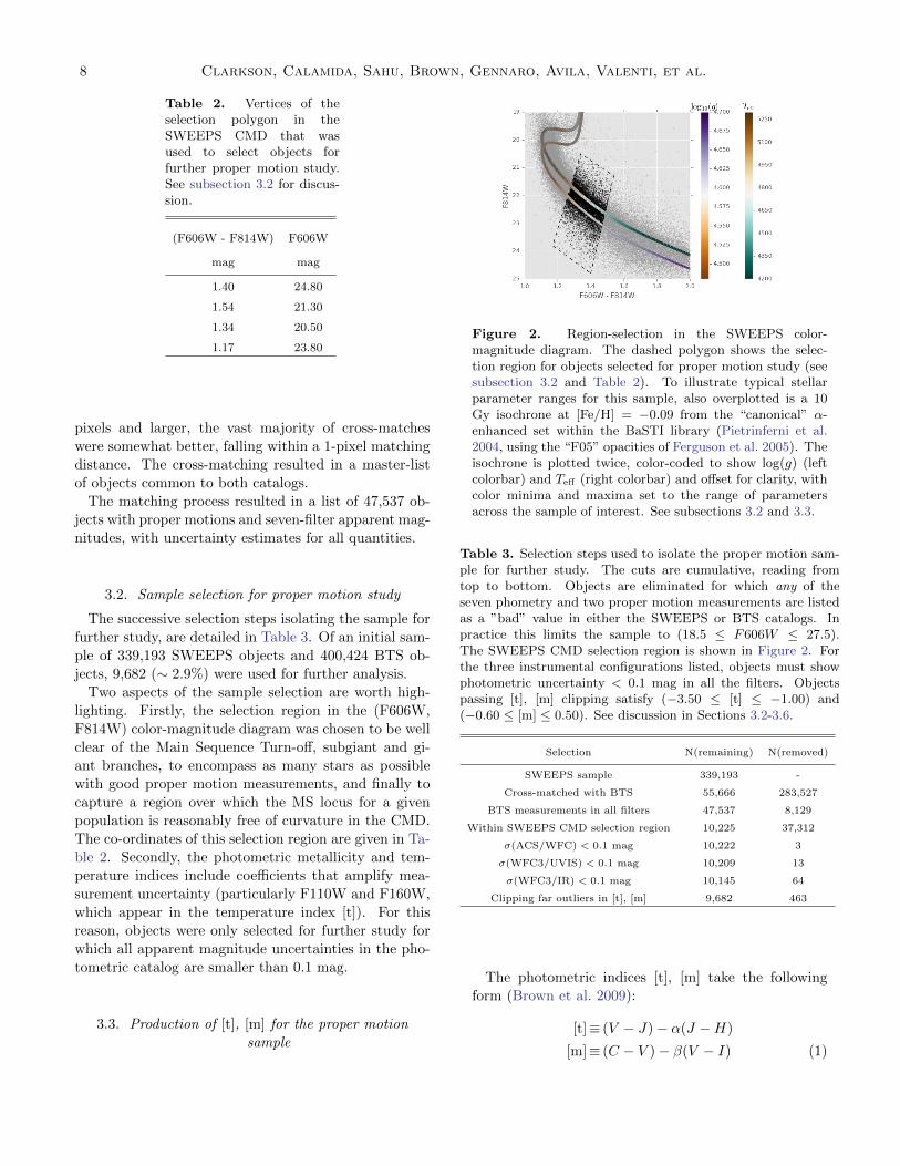
Table 2. Vertices of theselection polygon in theSWEEPS CMD that wasused to select objects forfurther proper motion study.See subsection 3.2 for discus-sion.

(F606W - F814W) F606W

mag mag

1.40 24.80

1.54 21.30

1.34 20.50

1.17 23.80

pixels and larger, the vast majority of cross-matches

were somewhat better, falling within a 1-pixel matching

distance. The cross-matching resulted in a master-list

of objects common to both catalogs.

The matching process resulted in a list of 47,537 ob-

jects with proper motions and seven-filter apparent mag-

nitudes, with uncertainty estimates for all quantities.

3.2. Sample selection for proper motion study

The successive selection steps isolating the sample for

further study, are detailed in Table 3. Of an initial sam-

ple of 339,193 SWEEPS objects and 400,424 BTS ob-

jects, 9,682 (∼ 2.9%) were used for further analysis.

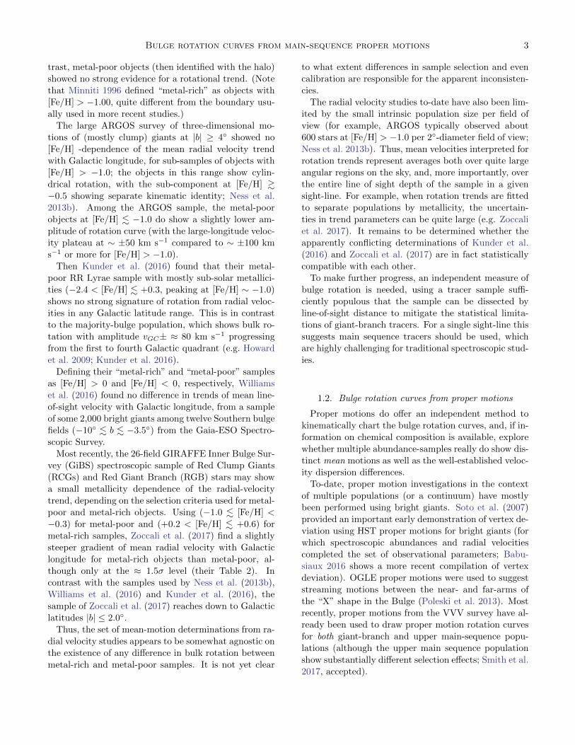
Two aspects of the sample selection are worth high-

lighting. Firstly, the selection region in the (F606W,

F814W) color-magnitude diagram was chosen to be well

clear of the Main Sequence Turn-off, subgiant and gi-

ant branches, to encompass as many stars as possible

with good proper motion measurements, and finally to

capture a region over which the MS locus for a given

population is reasonably free of curvature in the CMD.

The co-ordinates of this selection region are given in Ta-

ble 2. Secondly, the photometric metallicity and tem-

perature indices include coefficients that amplify mea-

surement uncertainty (particularly F110W and F160W,

which appear in the temperature index [t]). For this

reason, objects were only selected for further study for

which all apparent magnitude uncertainties in the pho-

tometric catalog are smaller than 0.1 mag.

3.3. Production of [t], [m] for the proper motion

sample

Figure 2. Region-selection in the SWEEPS color-magnitude diagram. The dashed polygon shows the selec-tion region for objects selected for proper motion study (seesubsection 3.2 and Table 2). To illustrate typical stellarparameter ranges for this sample, also overplotted is a 10Gy isochrone at [Fe/H] = −0.09 from the “canonical” α-enhanced set within the BaSTI library (Pietrinferni et al.2004, using the “F05” opacities of Ferguson et al. 2005). Theisochrone is plotted twice, color-coded to show log(g) (leftcolorbar) and Teff (right colorbar) and offset for clarity, withcolor minima and maxima set to the range of parametersacross the sample of interest. See subsections 3.2 and 3.3.

Table 3. Selection steps used to isolate the proper motion sam-ple for further study. The cuts are cumulative, reading fromtop to bottom. Objects are eliminated for which any of theseven phometry and two proper motion measurements are listedas a ”bad” value in either the SWEEPS or BTS catalogs. Inpractice this limits the sample to (18.5 ≤ F606W ≤ 27.5).The SWEEPS CMD selection region is shown in Figure 2. Forthe three instrumental configurations listed, objects must showphotometric uncertainty < 0.1 mag in all the filters. Objectspassing [t], [m] clipping satisfy (−3.50 ≤ [t] ≤ −1.00) and(−0.60 ≤ [m] ≤ 0.50). See discussion in Sections 3.2-3.6.

Selection N(remaining) N(removed)

SWEEPS sample 339,193 -

Cross-matched with BTS 55,666 283,527

BTS measurements in all filters 47,537 8,129

Within SWEEPS CMD selection region 10,225 37,312

σ(ACS/WFC) < 0.1 mag 10,222 3

σ(WFC3/UVIS) < 0.1 mag 10,209 13

σ(WFC3/IR) < 0.1 mag 10,145 64

Clipping far outliers in [t], [m] 9,682 463

The photometric indices [t], [m] take the following

form (Brown et al. 2009):

[t]≡ (V − J)− α(J −H)

[m]≡ (C − V )− β(V − I) (1)

Bulge rotation curves from main-sequence proper motions 9

with α ≡ E(F555W−F110W )/E(F110W−F160W ) and

β ≡ E(F390W − F555W )/E(F555W − F814W ), all of

which depend on stellar parameters. The median values

of these stellar parameters for the proper motion sample

(Teff ≈ 4800 K and log(g) ≈ 4.6) were estimated from

an isochrone chosen to overlap the observed sample (see

Figure 2; several combinations of metallicity, age and

extinction were tried, indicating that the parameter

range for this sample is roughly 4200 K. Teff . 5200 K

and 4.5 . log(g) . 4.7).

Figure 3. [t], [m] distribution of the population selected forproper motion study. In the main panel, green points showindividual objects, black contours show the smoothed repre-sentation as a two-dimensional KDE with ten levels plotted.Marginal distributions in [t] and [m] are shown in the top andright panels, respectively. Typical estimates for measure-ment uncertainty in this space are presented in Figure 18.See subsection 3.3.

3.4. Extinction estimates for reddening-free indices

The factors α, β are three-filter extinction ratios

(Brown et al. 2009). Synthetic photometry was used to

estimate the relationship between reddening and extinc-

tion for the objects of interest, and to generate reddening

vectors in the various filter combinations of interest. For

a range of E(B−V ) values, pysynphot was used to gen-

erate synthetic stellar spectra and the run of AX against

E(B − V ) was fit as AX = kXE(B − V ) separately for

all seven filters used in this study, over the range 0.0 ≤E(B−V )≤ 1.5. The calculation was performed for Teff ,

log(g) appropriate to the SWEEPS CMD region chosen

for proper motion study (Table 4). The process was re-

peated for low- and high-metallicity objects to estimate

sensitivity of the extinction prescription to metallicity

variation within the sample selected for further study,

and for (Teff , log(g)) for objects at the median, mini-

mum and maximum Teff within this sample to estimate

spread of α, β along the sample. For convenience, de-

rived quantities AF606W −AF814W and the scale factors

were also computed for MS objects.

This procedure requires a prescription for the extinc-

tion law towards the bulge. This extinction law ap-

pears to be somewhat non-standard and strongly spa-

tially variable, with some doubt in the literature about

whether a single-parameter model can accurately repro-

duce observed behavior from the visible to the near-

infrared (e.g. Nataf et al. 2016, and references therein).

As the [t], [m] indices use photometry in a very broad

color-range (CV IJH), systematic uncertainties in the

extinction prescription will in turn impact any infer-

ences about the underlying metallicity distribution (this

is one reason why we use [t], [m] only to classify objects

by relative [Fe/H] estimates).

To make progress, we adopted a single-parameter red-

dening law, but with ratio of selective to total extinc-

tion RV = 2.5, as suggested by the investigations of

Nataf et al. (2013).8 As this value is not among the

standard parameterizations available in pysynphot, the

coefficients AX/E(B − V ) for the seven filters were es-

timated for RV = 2.1 and RV = 3.1 and linearly inter-

polated to RV = 2.5.

Table 4 shows the adopted coefficients, along with

the derived values for the F606W-F814W color, and,

finally, the coefficients α, β in the [t], [m] indices. These

are quite different from the MS coefficients reported in

Brown et al. (2009), as expected since here we are tar-

geting a specific population some way beneath the Main

Sequence turn-off, and have used a different prescription

for extinction.

Within the sample of interest, the variation of all

extinction-relevant quantities appears to be small;

α, β each vary by < 0.1 between the two abundance-sets

tested, and, for a given abundance (and choice for RV ),

by . 0.02 across the Teff range of this sample. Here we

adopt (α, β) = (6.44, 1.10).

3.5. The [t], [m] distribution

The ([t], [m]) distribution of objects is shown in Fig-

ure 3. Two concentrations are apparent; one near ([t],

8 As a check, the entire kinematic analysis of Sections 3 & 4was also performed using RV = 3.1. Although the mean positionof objects in the [t], [m] diagram shifts slightly when RV = 3.1 isadopted instead of RV = 2.5, the kinematic trends for the “metal-rich” and “metal-poor” samples are similar.

10 Clarkson, Calamida, Sahu, Brown, Gennaro, Avila, Valenti, et al.

Table 4. Estimates of AX/E(B−V ) and derived parameters. Here Teff = 4800.0 and log(g) = 4.59. For convenience, the scalefactor for the SWEEPS color index is also shown. The quantities α, β give the extinction ratios relevant for [t], [m]. Specifically,α ≡ E(F555W −F110W )/E(F110W −F160W ) and β ≡ E(F390W −F555W )/E(F555W −F814W ). See subsection 3.3 andsubsection 3.4.

Config CCM89,RV = 2.1:log(Z)= -3.3

CCM89,RV = 2.1:log(Z)= -1.6

CCM89,RV = 3.1:log(Z)= -3.3

CCM89,RV = 3.1:log(Z)= -1.6

CCM89,RV = 2.5:log(Z)= -3.3

CCM89,RV = 2.5:log(Z)= -1.6

ACS/WFC1/F606W 1.847 1.849 2.786 2.788 2.222 2.224

ACS/WFC1/F814W 1.064 1.064 1.821 1.822 1.366 1.367

WFC3/UVIS1/F390W 3.507 3.492 4.489 4.475 3.899 3.885

WFC3/UVIS1/F555W 2.183 2.186 3.167 3.171 2.576 2.58

WFC3/UVIS1/F814W 1.074 1.075 1.833 1.834 1.377 1.378

WFC3/IR/F110W 0.560 0.558 1.025 1.021 0.746 0.743

WFC3/IR/F160W 0.345 0.345 0.635 0.634 0.461 0.460

(F606W-F814W)ACS/WFC1 0.784 0.785 0.965 0.966 0.856 0.857

α 7.55 7.64 5.49 5.56 6.42 6.49

β 1.19 1.18 0.99 0.98 1.10 1.09

[m]) = (-2.0, 0.15), with a second, more elongated con-

centration with major axis angled at about −45◦ in Fig-

ure 3, centered near ([t], [m]) ≈ (−2.2,−0.1).

Figure 4 shows an attempt to reproduce the distribu-

tion of [m] only as a Gaussian Mixture Model (GMM;

see Appendix A for discussion of the technique). At

least two components seem to be required, although the

data do not discriminate between the simplest model

that fits the data (two components) and a continuum

(e.g. 8 components).

In early trials using data selected only on photo-

metric measurement uncertainty, a mixture model with

more than three components would usually include an

extremely broad, low-significance Gaussian component.

On plotting the [m] counts on a log-scale, this compo-

nent was seen to be fitting handfuls of far outliers in

the [m] distribution (with |[m]| > 0.5; compare with the

range in Figure 4). This may be expected if the outliers

are not well-represented by the model form; neverthe-

less, the GMM implementation would attempt to assign

a model component to the outliers once the model grew

sufficiently complex, which in turn would distort model

components much nearer to the location of the main

population of objects. Circumventing this outlier prob-

lem was the main motivator for outlier removal in [t],

[m] when selecting objects for further analysis (Table 3).

3.6. Classifying samples in [t], [m]

To draw “metal-rich” and “metal-poor” samples from

the population selected for rotation curve extraction

(Figure 2), the population was characterized as a Gaus-

sian Mixture Model (GMM) in ([t], [m]) space, and

members of the “metal-poor” and “metal-rich” sam-

ples identified by their formal membership probability

wik (see Appendix A).

Figure 5 shows the ([m], [t]) GMM characterization

of the population. To examine the impact of changing

the number of model components K, the [t], [m] data

were split into two equal-size samples (the “training”

and “test” sets), and the GMM fit using the “train-

ing” set. Samples (of [t], [m]) were then drawn from

the model and perturbed by measurement covariances

Si from the “test” set, and the ([t], [m]) distribution of

this predicted set compared with the “test” set. The

GMM predicts distributions slightly more centrally con-

centrated than the true distribution, but for K = 4 the

residual “images” do not suggest the presence of a miss-

ing model component (Figure 5). Repeated trials using

K = 3 model components consistently showed that the

three-component model typically leaves a strong resid-

ual at ([t], [m]) ≈ (−2.2,−0.15) that is not present with

K = 4, while the formal fit statistics appear somewhat

worse for K = 3 than for K = 4. We therefore adopt a

four-component Gaussian Mixture Model to character-

ize the observed distribution in [t], [m] space for the rest

of this work.

Table 5 presents the parameters of the adopted four-

parameter GMM prescription for the [t], [m] distribu-

tion. As [t], [m] each represent three-filter flux ratios

expressed in logarithmic units, subject to systematics

both in absolute calibration and in extinction prescrip-

tion, the translation from [t], [m] to absolute Teff and

[Fe/H] is somewhat non-trivial and subject to system-

atic uncertainty; throughout this work, our goal is to

characterize the observed distribution of objects in or-

Bulge rotation curves from main-sequence proper motions 11

Figure 4. Left panel: distribution of [m], for objects satisfying −2.8 ≤ [t] ≤ −1.4, representing roughly the populationwithin the outer contour in Figure 3. The gray shaded region shows the observed [m] distribution. The upper gray solid lineshows a Gaussian Mixture Model trained on the [m] distribution. The colored solid and dashed curves show realizations of theindividual model components. Middle panel: as in the left panel, but with an eight-component Gaussian mixture specified asan ansatz for a continuum of populations. Right panel: Formal assessment of the number of parameters required to reproducethe observed [m] distribution. Standard figures of merit, the Bayesian Information Criterion (BIC, black dashed line) and theAkiake Information Criterion (AIC, gray solid line; see e.g. Ivezic et al. 2014) are plotted as a function of the number of modelcomponents. A GMM representation of the [m] distribution seems to require at least two components, with little improvementfor more complex models. See subsection 3.3.

Figure 5. Gaussian Mixture Model (GMM) of the population selected for rotation curve study. The first three columns showHess diagrams in ([t], [m]) space, using using K = 3 (top row) and K = 4 (bottom row) mixture components. Left panelsshow the histogram of samples drawn from a GMM fit to a randomly selected sample of half the data (the “training set”). Themiddle-left panels show the other half of the data (the “test set”), with the 1σ contours of the model components overplotted asthick cyan ellipses. The middle-right panels show the residuals (samples from the model minus the observed counts in the “testset”). The lower-right plot shows formal fit statistics as a function of the number of model components. See subsection 3.6.

der to draw samples near the extremes of the underlying

relative abundance distribution.9

A rough estimate for the centroid [Fe/H] values of the

two samples may be drawn by charting [Fe/H] contours

9 Throughout this paper, the two samples are indicated withinverted commas to remind the reader of the limited scope of ourinterpretation of the “metal-rich” and “metal-poor” samples.

in the [t], [m] diagram for synthetic stellar populations

and interpolating to estimate [Fe/H] at the [t], [m] lo-

cations of the model component centroids (see subsec-

tion E.1 for more details on the synthetic stellar pop-

ulations used). The GMM component centroids pre-

sented in Table 5 correspond to [Fe/H]0 ≈ +0.18 for the

“metal-rich” sample (using scaled-to-solar isochrones)

and [Fe/H]0 ≈ −0.24 for the “metal-poor” sample (us-

12 Clarkson, Calamida, Sahu, Brown, Gennaro, Avila, Valenti, et al.

Table 5. Parameters of the Gaussian Mixture Model in [t],[m] space for stars beneath the main sequence selected for fur-ther study. Reading left-right, columns indicate the componentindex k, its label (if any), its (rounded) mixture fraction αk, thetwo components of its centroid, and the three unique componentsof the covariance matrix Vk. See subsection 3.5.

k Name αk [t]0 [m]0 σ2[t][t] σ2

[m][m] σ2[t][m]

mag mag (mag2) (mag2) (mag2)

0 “metal-poor” 0.580 -2.26 -0.09 0.0451 0.0149 -0.00747

3 “metal-rich” 0.334 -2.05 0.16 0.0368 0.0039 -0.00225

1 - 0.031 -1.42 -0.05 0.0215 0.0385 0.00043

2 - 0.055 -2.96 0.02 0.0301 0.0261 -0.00396

ing α-enhanced isochrones for this model component).

These centroids are roughly consistent with values sug-

gested from spectroscopic surveys (e.g. Zoccali et al.

2017; Hill et al. 2011).

It is important to remember that we are not at this

stage suggesting that the bulge sample of BTS is indeed

bimodal in metallicity (as opposed to a continuum of

populations, e.g. Gennaro et al. 2015; Debattista et al.

2017). Instead, we are using the photometric indices

[t], [m] to draw samples near the extremes of relative

abundance.

For an object to be classified with the “metal-rich” or

“metal-poor” sample, it must show formal membership

probability wik ≥ 0.7 (Equation A1; note that an object

need not be classified with either sample when there

are four model components), using uncertainty prop-

agation to approximate the suitable measurement co-

variance matrix for each object (see Figure 6 and Ap-

pendix A).

The threshold wik ≥ 0.7) was chosen as a tradeoff be-

tween sample purity (typical objects should not fall into

more than one model component at the chosen thresh-

old) and the need to have a sufficient sample size (at

least a few thousand) to permit the dissection of the

proper motions by relative photometric parallax with

sufficient resolution to chart the rotation curves.

The fiducial ridgelines for photometric parallax were

determined by a simple empirical fit to the mean “metal-

rich” and “metal-poor” samples in the SWEEPS CMD.

A second-order polynomial fit adequately represents the

median samples, and allows very rapid evaluation of rel-

ative photometric parallax. Figure 6 shows the samples

identified with all four GMM model components, while

Figure 7 shows the adopted loci for the “metal-rich” and

“metal-poor” samples. The parameters of the loci them-

selves are given in Table 6.

Figure 6. Drawing samples by relative abundance, using lo-cation in ([t], [m])-space. The top row shows the [t], [m] sam-ple color-coded by membership probabilities wik (Equa-tion A1) for the k’th model component in the GMM char-acterization of the observed distribution. The 1σ ellipse forthe k’th model component is overplotted in each case as acolored ellipse. The bottom row plots the (F606W, F814W)color-magnitude diagram for samples with wik > 0.7 in eachcomponent. Reading left-right, the columns describe popu-lations identified with the “metal-poor” sample (blue in allfigures in this paper), the “metal-rich” (red in all figures),and the two populations that appear to fit different regionsof the background. See the discussion in subsection 3.6.

Table 6. Ridgeline parameters in theSWEEPS color-magnitude diagram, for the“metal-poor” and “metal-rich” samples.These purely empirical ridgelines are usedto rapidly evaluate photometric parallax forobjects in each sample, and take the formF814W = Σjajx

j with x the (F606W-F814W) color. See subsection 3.6 for discus-sion.

k Name a0 a1 a2

mag (mag−1)

1 “metal-poor” -19.855 53.335 -16.904

3 “metal-rich” 3.256 20.520 -5.679

3.7. Rotation curves

Armed with “metal-rich” and “metal-poor” samples

from the BTS photometry, along with mean fiducial se-

quences in the SWEEPS color-magnitude diagram for

the two samples, the next step is to chart their proper

motion rotation curves. Figure 8 shows the raw distri-

bution of longitudinal proper motion µl with relative

photometric parallax for the “metal-rich” and “metal-

poor” samples. The behavior against Galactic longitude

is characterized in Figure 9.

Bulge rotation curves from main-sequence proper motions 13

Figure 7. Ridgelines for the “metal-rich” and “metal-poor” samples. The grayscale shows the ACS/WFC(F606W,F814W) Hess diagram for the larger SWEEPS sample.Objects falling within the region of interest for our kine-matic study are presented as points, color-coded by “metal-rich” (red) or “metal-poor” (blue). The empirical median-sample ridgelines for the “metal-rich” (red solid) and “metal-poor” (blue dashed) are overlaid. See subsection 3.6 andTable 6.

Figure 8. Raw distribution of µl against relative photo-metric parallax (π′), for the “metal-rich” (red) and “metal-poor” (blue) populations. In each figure, the points them-selves are illustrated by colored scatterplots in the main pan-els, with density contours indicated in grayscale. In bothfigures, the top- and right-panels show the marginal distri-butions of π′(top panels) and µl (right panels). See subsec-tion 3.7.

Figure 9. The raw µl distributions against relative pho-tometric parallax (see Figure 8). “metal-rich” is denotedin red in the top-panel, “metal-poor” in blue in the bot-tom panel. The population is broken into bins in relativedistance-modulus and the median value µl determined foreach bin (triangles). Faint continuous lines show a third-order smoothed spline approximation fit to the binned propermotions µl, while squares indicate equally-spaced evaluationsof the spline approximation over the range of relative moduli(−1.0 ≤ (m−m0) < +1.0). See subsection 3.7.

Several general differences are apparent between the

samples. Firstly, there is a general sense of rotation in

both samples, with the foreground showing positive µl,

changing to negative µl on the far side, although the

amplitude of the difference is roughly a factor 2 higher

for the “metal-rich” sample. Secondly, the “metal-

poor” sample shows greater spread in relative photo-

metric parallax (π′).

3.8. Proper motion ellipse dissected by relative

photometric parallax

With a difference in rotation curves suggested from

the behavior of µl against relative photometric parallax,

we can move to a greater level of sophistication and chart

the distance-variation of the (l, b) proper motion ellipse.

The approach shares several similarities to that reported

in Cl08; relative photometric parallaxes were assigned

to each star with reference to the fiducial sequence (ap-

propriate for the metallicity-sample from which the star

is drawn) and the sample partitioned into bins of rela-

tive photometric parallax π′, with bin-widths adjusted

so that each bin has the same number of objects.

14 Clarkson, Calamida, Sahu, Brown, Gennaro, Avila, Valenti, et al.

The proper motion distribution within each bin was fit

as a two-dimensional Gaussian, centered at ~µ0 and with

covariance matrix Vµ. Uncertainties in fitted quantities

were estimated by parametric bootstrapping: synthetic

samples for each bin were drawn from the best-fit model,

perturbed by the estimated proper motion uncertainty,

and the distribution of recovered parameters over the

bootstrap trials adopted as the estimated parameter un-

certainties. Because the GMM method can be sensitive

to outliers, a single pass of sigma-clipping was applied

to the proper motion sample within each distance bin

using a ±3σ threshold; this typically removed roughly

1-2% of the points per bin, with the exeption of the most

distant π′ bin (see Tables 15 & 16).

Several improvements have been made over the anal-

ysis reported in Cl08. For example, rather than sub-

tracting the estimated proper motion uncertainty in

quadrature from the model covariances after fitting,

the “extreme deconvolution” formulation of Bovy et al.

(2011) was used, which incorporates estimated mea-

surement uncertainty as part of the fitting process (see

Appendix A). The estimates of proper motion uncer-

tainty themselves have also been improved compared to

Cl08, in both the characterization of random uncertainty

through the artificial star tests of Ca15 and through

improved characterization of residual relative distortion

(Kains et al. 2017). Details of the uncertainty esti-

mates we adopt here are presented in subsection A.2; for

the apparent magnitude range of interest here, the to-

tal proper motion uncertainty estimates (εi . 0.13 mas

yr−1) are much smaller than the intrinsic proper motion

dispersion of the bulge (∼ 3 mas yr−1).

4. RESULTS

4.1. Rotation curves for the “metal-rich” and

“metal-poor” samples

The trends in observed motions are shown graphically

in Figures 10 - 12, while Figure 13 shows the trends

after conversion from relative photometric parallax and

proper motion to distance and velocity. This informa-

tion is presented in tabular form in Appendix G.

The distance conversion assumes the mean popula-

tion lies at distance modulus (m−M)0 = 14.45 (Ca14),

converting to a reference distance (D0 = 7.76 kpc) and

assigning this distance to the ridgelines for the “metal-

rich” and “metal-poor” samples.

Consistent with the simple treatment in Figure 9

and subsection 3.7, the “metal-rich” sample shows a

higher-amplitude rotation curve than does the “metal-

poor” sample, both with a steeper slope and about a

factor ∼ 2 greater difference in 〈vl〉 between nearside

Figure 10. Variation of proper motion centroid with rela-tive photometric parallax, for “metal-rich” (red triangles)and “metal-poor” (blue circles) samples, using a binningscheme with 200 objects per bin. The top row shows theproper motion centroid in Galactic longitude, the bottomrow shows the proper motion centroid in Galactic latitude.Errorbars show 1σ uncertainties from parametric bootstrap-ping, using the best-fit parameters and measurement uncer-tainties to generate 1000 trial datasets for each distance bin.See subsection 4.1.

Figure 11. Semimajor (top) and semiminor (bottom) axis-lengths for the proper motion ellipse. Symbols, colors anderrorbars as for Figure 10. See subsection 4.1.

Bulge rotation curves from main-sequence proper motions 15

Figure 12. Variation of the proper motion ellipse axis ratio(top) and the position angle of its major axis (bottom) asa function of relative photometric parallax. Position angleθ = 0◦ would mean the proper motion ellipse major axisaligns with the Galactic longitude axis. Symbols as Fig-ure 10, with the “metal-poor” sample shown more faintly toavoid cluttering the plots. See subsection 4.1.

and farside of the bulge than for the “metal-poor” sam-

ple.

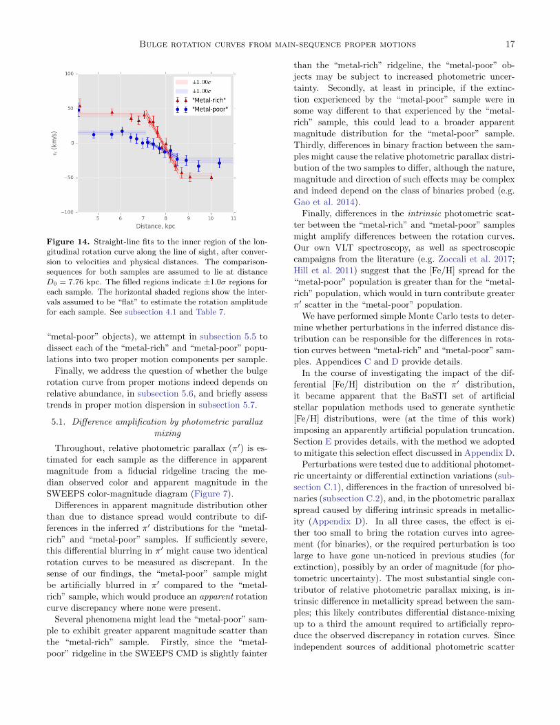
To quantify the rotation curve discrepancies between

the samples, a simple straight-line model was fit to the

rotation curves over the inner distance range (6.4 ≤ D ≤8.0 kpc). Since the “metal-rich” rotation curve visu-

ally appears to level off at smaller |π′| than the “metal-

poor” sample, the rotation curves to both samples were

characterized over the same range in distance modulus.

The 1σ ranges of 〈µl〉 and 〈vl〉 from the parametric boot-strap trials were used as estimates of measurement un-

certainty in each distance-bin, and the inverse variance-

weighted mean value of π′ and D subtracted from the

distance co-ordinates to minimze covariance in the fit-

ted parameters. Trends were fitted to each of the (π′,

〈µl〉) and (D, 〈vl〉) rotation curves separately (rather

than transforming the proper motion trends into veloc-

ity trends after fitting). We did not attempt to deproject

velocities to circular speeds (as discussed in Cl08) but

merely attempted to characterize observed trends.

Figure 14 and Table 7 show the results. The difference

in slopes is ∆(dvl/dD) = −41.0±7.5 km s−1 kpc−1 while

the ratio of amplitudes is AMR/AMP = 2.2±0.3. Thus,

a difference in rotation curve slopes is detected at ap-

proximately 5.5σ while a multiplication factor in the am-

plitude is detected at approximately 8.1σ.

Both the simple decomposition (subsection 3.7) and

the fits of proper motion ellipses (subsection 3.8) suggest

that the two rotation curves might intersect at slightly

negative mean motion and slightly on the far-side of the

Bulge (e.g. the right column of Figure 14). Since the

proper motions are determined relative to the average

observed bulge proper motion, across all metallicities,

the proper motion zeropoint is therefore dependent on a

range of selection and projection effects (see, for exam-

ple, Ca14; Cl08, and Appendix A of Lopez-Corredoira

et al. 2007). Thus it is not surprising that the two se-

quences do not necessarily meet at (π′, µl) = (0.0, 0.0).

The latitudinal motion curve (Figure 10, bottom

panel) visually suggests a gentle trend from nearside

to farside, consistent with previous measurements (e.g.

Cl08, Soto et al. 2014). The behaviors of the two sam-

ples in µb are statistically similar, with slopes dvb/dD =

−2.40±9.80 km s−1 kpc−1 and dvb/dD = 22.4±6.53 km

s−1 kpc−1 for the “metal-rich” and “metal-poor” sam-

ples, respectively, corresponding to a slope difference

of 20.0 ± 11.8 km s−1 kpc−1. The samples have am-

plitude ratio 9.5/5.1 = 1.86 ± 1.35, which we do not

consider to be a secure detection of differing rotation

curve amplitude in the latitudinal direction.

4.2. Proper motion ellipse morphology and amplitudes

The velocity dispersion profiles (measured as major

and minor axis lengths of the proper motion and ve-

locity ellipsoids; Figures 11 & 13) also show differences

between the samples. Both samples show a broadly

centrally-peaked velocity dispersion pattern against line-

of-sight distance (Figure 13), with the “metal-rich” sam-

ple showing a narrower peak, particularly in the major-

axis dispersion. The “metal-rich” sample also shows

generally lower velocity dispersion by ∼ 10%, partic-

ularly in terms of the velocity ellipse minor axis.

Consistent with previous studies (e.g. Soto et al.

2014), the proper motion ellipse appears to be weakly

elongated, with the “metal-rich” population possibly

the more elongated of the two samples (with axis-ratio

b/a ≈ 1.25 at π′ = 0 compared to b/a ≈ 1.1; see the

top panel of Figure 12). The “metal-rich” population

may show increased elongation for sample bins near the

median distance.

The proper motion ellipse major axis position angle

also shows trends with relative photometric parallax,

although possibly at lower statistical significance than

the trends reported in Cl08 despite a much longer time-

baseline for proper motions (Ca14). This reduced sig-

nificance may be due to the reduced sample size admit-

ted by the cuts in [t], [m] employed in this work. It

may be that only the “metal-rich” sample substantially

16 Clarkson, Calamida, Sahu, Brown, Gennaro, Avila, Valenti, et al.

Figure 13. Transverse velocity ellipse centroids (left column) and axis lengths (right column) as a function of estimated line ofsight distances. Symbols as Figures 10 & 11, except distance moduli have been converted to line of sight distances, and propermotions converted to velocities in km s−1. See subsection 4.1.

Table 7. Trend parameters for the inner Bulge region. See subsection 4.1.

Sample Gradient (µl) Amplitude (µl) Gradient (vl) Amplitude (vl)

(mas yr−1 mag−1) (mas yr−1) (km s−1 kpc−1) (km s−1)

”Metal-poor” −1.54± 0.37 0.49± 0.06 −16.7± 3.65 20.2± 2.25

”Metal-rich” −5.65± 0.61 1.20± 0.06 −57.7± 6.49 44.0± 2.29

shows the proper motion ellipse tilt with distance, with

position angle rising to the 20◦ − 40◦ range (this tilt

is strongly influenced by projection effects; see Section

5.1 and particularly equation (2) of Cl08 for discussion

of these effects). Because the “metal-poor” population

tends to be less elongated, its position angle trends are

also detected at lower significance.

The very nearest relative photometric parallax bins

show behavior consistent with a foreground population

dominated by Galactic rotation. This seems particularly

clear for the “metal-rich” sample, which shows a much

more strongly elongated proper motion ellipse for the

nearest bin (a/b ≈ 1.9 ± 0.26) and position angle con-

sistent with zero (consistent with differential rotation in

Galactic latitude).

5. DISCUSSION

The trends indicated by the union of the BTS and

SWEEPS datasets, particularly the rotation curves (pre-

sented in Figures 9, 10 & 13), are quite striking. The

“metal-rich” rotation curve appears to show systemati-

cally greater rotation amplitude than the “metal-poor”

sample, shows a greater degree of central concentration

along the line of sight (see Figure 13 as well as the raw

distributions in Figure 8), and may show systematically

lower velocity dispersion (Figure 13).

Before attempting to interpret the trends, however, weexamine the magnitude and impact of several potential

systematics that might bias the samples, whether by

amplifying or even artificially generating the apparent

trends in rotation curve (subsection 5.1), or by reduc-

ing them due to mixing in the ([t], [m]) space used to

draw the “metal-rich” and “metal-poor” samples (sub-

section 5.2).

Implications of the relative photometric parallax dis-

tributions for the spatial distributions of the “metal-

rich” and “metal-poor” samples are discussed in subsec-

tion 5.3, while subsection 5.4 discusses the implications

of our results for the traditional selection of a “clean-

bulge” sample using cuts on longitudinal proper motion

µl.

Because a metal-poor kinematically-hot “Classical

bulge” and/or “halo” bulge component may be present

in the inner Milky Way (perhaps more likely among

Bulge rotation curves from main-sequence proper motions 17

Figure 14. Straight-line fits to the inner region of the lon-gitudinal rotation curve along the line of sight, after conver-sion to velocities and physical distances. The comparison-sequences for both samples are assumed to lie at distanceD0 = 7.76 kpc. The filled regions indicate ±1.0σ regions foreach sample. The horizontal shaded regions show the inter-vals assumed to be “flat” to estimate the rotation amplitudefor each sample. See subsection 4.1 and Table 7.

“metal-poor” objects), we attempt in subsection 5.5 to

dissect each of the “metal-rich” and “metal-poor” popu-

lations into two proper motion components per sample.

Finally, we address the question of whether the bulge

rotation curve from proper motions indeed depends on

relative abundance, in subsection 5.6, and briefly assess

trends in proper motion dispersion in subsection 5.7.

5.1. Difference amplification by photometric parallax

mixing

Throughout, relative photometric parallax (π′) is es-

timated for each sample as the difference in apparent

magnitude from a fiducial ridgeline tracing the me-

dian observed color and apparent magnitude in the

SWEEPS color-magnitude diagram (Figure 7).

Differences in apparent magnitude distribution other

than due to distance spread would contribute to dif-

ferences in the inferred π′ distributions for the “metal-

rich” and “metal-poor” samples. If sufficiently severe,

this differential blurring in π′ might cause two identical

rotation curves to be measured as discrepant. In the

sense of our findings, the “metal-poor” sample might

be artificially blurred in π′ compared to the “metal-

rich” sample, which would produce an apparent rotation

curve discrepancy where none were present.

Several phenomena might lead the “metal-poor” sam-

ple to exhibit greater apparent magnitude scatter than

the “metal-rich” sample. Firstly, since the “metal-

poor” ridgeline in the SWEEPS CMD is slightly fainter

than the “metal-rich” ridgeline, the “metal-poor” ob-

jects may be subject to increased photometric uncer-

tainty. Secondly, at least in principle, if the extinc-

tion experienced by the “metal-poor” sample were in

some way different to that experienced by the “metal-

rich” sample, this could lead to a broader apparent

magnitude distribution for the “metal-poor” sample.

Thirdly, differences in binary fraction between the sam-

ples might cause the relative photometric parallax distri-

bution of the two samples to differ, although the nature,

magnitude and direction of such effects may be complex

and indeed depend on the class of binaries probed (e.g.

Gao et al. 2014).

Finally, differences in the intrinsic photometric scat-

ter between the “metal-rich” and “metal-poor” samples

might amplify differences between the rotation curves.

Our own VLT spectroscopy, as well as spectroscopic

campaigns from the literature (e.g. Zoccali et al. 2017;

Hill et al. 2011) suggest that the [Fe/H] spread for the

“metal-poor” population is greater than for the “metal-

rich” population, which would in turn contribute greater

π′ scatter in the “metal-poor” population.

We have performed simple Monte Carlo tests to deter-

mine whether perturbations in the inferred distance dis-

tribution can be responsible for the differences in rota-

tion curves between “metal-rich” and “metal-poor” sam-

ples. Appendices C and D provide details.

In the course of investigating the impact of the dif-

ferential [Fe/H] distribution on the π′ distribution,

it became apparent that the BaSTI set of artificial

stellar population methods used to generate synthetic

[Fe/H] distributions, were (at the time of this work)

imposing an apparently artificial population truncation.

Section E provides details, with the method we adopted

to mitigate this selection effect discussed in Appendix D.

Perturbations were tested due to additional photomet-ric uncertainty or differential extinction variations (sub-

section C.1), differences in the fraction of unresolved bi-

naries (subsection C.2), and, in the photometric parallax

spread caused by differing intrinsic spreads in metallic-

ity (Appendix D). In all three cases, the effect is ei-

ther too small to bring the rotation curves into agree-

ment (for binaries), or the required perturbation is too

large to have gone un-noticed in previous studies (for

extinction), possibly by an order of magnitude (for pho-

tometric uncertainty). The most substantial single con-

tributor of relative photometric parallax mixing, is in-

trinsic difference in metallicity spread between the sam-

ples; this likely contributes differential distance-mixing

up to a third the amount required to artificially repro-

duce the observed discrepancy in rotation curves. Since

independent sources of additional photometric scatter

18 Clarkson, Calamida, Sahu, Brown, Gennaro, Avila, Valenti, et al.

would presumably add in quadrature, their combination

is very unlikely to be sufficient to bring about the ob-

served discrepancies in trends.

We therefore conclude that differential distance scat-

ter is not responsible for the difference in rotation curves

or π′ distributions, due to additional photometric un-

certainty, differential extinction, differences in the unre-

solved binary populations, or in the differences in metal-

licity spread between samples.

5.2. Difference reduction by sample

cross-contamination

While blurring in relative photometric parallax would

tend to artificially increase the difference between trends

in the “metal-rich” and “metal-poor” samples, cross-

contamination of the samples in ([t], [m]) would tend

to artificially reduce these differences. While we have

used reasonably conservative thresholds in drawing

our “metal-rich” and “metal-poor” samples, genuinely

metal-rich objects might be moved into the “metal-

poor” sample by measurement uncertainty, and vice

versa.

Because of the complexities involved in rigorous re-

construction of the observed distributions (e.g. Gennaro

et al. 2015), full exploration of this cross-contamination

is deferred to future work. We have performed a simple

Monte Carlo contamination test for the formal member-

ship probability threshold wik > 0.7 used in this work

(Appendix F).

Under the assumptions of that test, we find that the

“metal-rich” sample is contaminated at the ∼ 8% level

(about half from the “metal-poor” sample), while the

“metal-poor” sample is contaminated at the ∼ 5% level

(with . 0.5% due to the “metal-rich” sample). This is

likely not severe enough for the observed low-amplitude

“metal-poor” rotation curve to be entirely due to sam-

ple contamination from a small population of objects

following the kinematics of the “metal-rich” sample.

5.3. The line of sight distance distributions of the two

samples

The tendency of the “metal-poor” sample to show

greater dispersion in relative photometric parallax (or,

correspondingly, in distance D), is qualitatively consis-

tent with the “kinematic fractionation” of Debattista

et al. (2017). Identifying a “metal-poor” sample with

an older population, this difference in line-of-sight dis-

tance distribution would also be qualitatively consistent

with the observations of Catchpole et al. (2016), who

find differing bar angles and degrees of central concen-

tration for Mira variables of different ages. However,

how the predictions of Catchpole et al. (2016) translate

into predictions for the two samples here, is deferred to

future work.

5.4. Implications for proper motion selection

Photometric studies of the Bulge typically impose a

condition µl < −2.0 mas yr−1 to isolate a clean bulge

sample for further study (e.g. Kuijken & Rich 2002;

Calamida et al. 2014). This procedure is appropri-

ate because in the sight-lines typically studied near the

Galactic center, the foreground disk population typically

shows proper motion relative to the mean-bulge popu-

lation of ∆µl ≈ +4 mas yr−1, as suggested by direct

comparison of the proper motions of bulge giant branch

stars with those of the upper main-sequence population

of (mostly) disk foreground stars (e.g. Cl08, Soto et al.

2014).

To investigate whether and how this cut imposes se-

lection effects on the two samples, we computed the

sample counts, fractions and volume densities for ob-

jects that would pass the longitudinal proper motion cut

(µl < −2.0 mas yr−1). The results are plotted in Fig-

ure 15 and presented in tabular form in Appendix G.

We find that the cut (µ < −2.0 mas yr−1) admits very

few foreground objects from either sample; both samples

show fewer than four objects passing this cut for the clos-

est distances (d . 4.49 kpc and . 4.25 kpc for “metal-

rich” and “metal-poor” samples, respectively, corre-

sponding to the closest single and the closest two bins

respectively; see Table 15 and Table 16 in Appendix G),

while the foreground population’s mean proper motion

〈µl〉 climbs strongly for the closest distance bins (Fig-

ure 10). We therefore confirm that the traditional

proper motion cut (µ < −2.0 mas yr−1) does indeed

remove nearby objects cleanly for the SWEEPS field.10

Beyond this, however, the dissection by relative abun-

dance has revealed several interesting selection effects

among the kinematically-cleaned sample (Figure 15).

Firstly, as expected, there is a bias towards the far side

of the bulge, but this bias is much stronger in the “metal-

rich” sample than for the “metal-poor”; indeed the frac-

tion of “metal-poor”objects passing the kinematic cut is

almost flat with inferred distance between d . 5 kpc

. 9 kpc.

Secondly, the raw counts of sources thus isolated in the

“metal-rich” and “metal-poor” samples are of similar or-

10 Strictly speaking, the classification of the nearest objects into“metal-rich” and “metal-poor” samples may suffer different selec-tion effects to the rest of the samples because either or both of thestellar parameters and extinction might be different for the verynearest objects compared to the majority sample at more bulge-like distances. We are making the assumption that the relativeclassification of objects in the nearest distance bins, is still valid.

Bulge rotation curves from main-sequence proper motions 19

Figure 15. Selection functions imposed by the traditional kinematic cut µl ≤ −2.0 mas yr−1, for the “metal-rich” (red triangles,solid line) and “metal-poor” (blue circles, dashed line) samples. Left column: volume density of all objects assigned to eachsample (left-top) and which would pass the kinematic cut (bottom panel). Right column: number of objects per sample thatwould pass the kinematic cut (right-top) and the fraction (right-bottom) that would pass the cut. Each distance bin has thesame number of detected objects by construction (subsection 3.8), so bootstrap uncertainty estimates are not applicable to thetop-left panel. Because of this binning scheme, bins with the same counts generally do not indicate the same volume density ofdetected objects (between bins or between samples). The shaded yellow region represents inferred distances (6.5 ≤ d ≤ 9.0) kpc.For discussion, see subsection 5.4.

ders of magnitude. Considering sample sizes that pass

the kinematic cut at inferred distances between 6.4 and

9.1 kpc (chosen to encompass the bulge populations; see

Tables 15 and 16), the total counts in each sample are

566± 20 and 552± 20 for the “metal-rich” and “metal-

poor”samples, respectively (the uncertainties, estimated

from the quadrature sum of parametric bootstrap un-

certainty estimates in these counts for each bin, are al-

most certainly underestimates). With total sample sizes

within this distance range of 2381 (1984) for the “metal-

rich” (“metal-poor”) samples, this translates into frac-

tions 24%±1% (28%±1%) of the “metal-rich” (“metal-

poor”) samples that pass the kinematic cut. Thus, of

objects in this distance range, the kinematic cut appears

to slightly favor the “metal-poor”sample, although the

difference is small.

In principle, a population of compact objects among

the foreground population, might fall into the farther

distance-bins for the “metal-poor” sample 11, polluting

a sample with bulge-like motions with a small popula-

11 At colors typical of the “metal-poor” sample, the quiescentdwarf novae found by Ca14 at the distance of the bulge showF606W ∼ 28. Similar objects in a very nearby foreground diskpopulation (. 3 kpc) might fall within the faintest bins of ourchosen sample.

tion showing disk-like motions. However, with the fore-

ground disk population at ∼ 10− 15% of the total, and

with a substantial WD population perhaps unlikely for a

typical “young” foreground population, we do not con-

sider this a significant contaminant, and leave explo-

ration of the impact of foreground WDs to future work.

5.5. Are the metallicity-samples themselves composite?

In addition to any continuous metallicity-velocity cor-relation, the samples may include populations from dis-

tinct entities within the Bulge region, whether interloper

populations from the Halo (e.g. Koch et al. 2016) or any

Thick-disk component (e.g. Ness et al. 2013a) or a small

“Classical” bulge component (Kunder et al. 2016).

We have therefore performed the exercise of decom-

posing each of the “metal-rich” and “metal-poor” sam-

ples into two-component GMM’s (in µl only), to de-

termine if any minority component is distinguishable

within the rotation curves formed from the two samples

(figures 16 & 17).

No minority population is detected in either sample;

indeed, when a two-component GMM is used, the two

centroids track the mean rotation curve within each

sample roughly symmetrically about the mean rotation

curve, each sub-component has roughly equal weight in

the mixture.

20 Clarkson, Calamida, Sahu, Brown, Gennaro, Avila, Valenti, et al.

Figure 16. Representation of the “metal-poor” rotation curve as a two-component GMM in µl, to test the hypothesis thatthe “metal-poor” sample might itself be composite. Left column: rotation curve in µl as tracked by the two model components(left top), and the relative weights of the two model components (left bottom). Large dots indicate the more populous of thetwo model components in each bin (αk = 0.75 would mean three quarters of the sample came from model component k). Thegray line in the left-top panel shows the rotation curve inferred using a single model component at each distance-bin. Rightcolumn: µl distribution for the bin indicated for the shaded distance-bin in the left-column. Right top: µl distribution (shadedhistogram and thin black line), with the prediction of the two-component GMM (the thick and thin blue lines indicate the more-and less-populous model component, respectively, while the blue dashed line indicates the sum of the two). The gray thick lineshows the prediction of the single-component model. The bottom left and bottom right panels show the vector point diagramand distance modulus distribution, respectively. See subsection 5.5.

Figure 17. Representation of the “metal-rich” rotation curve as a two-component GMM in µl, to test the hypothesis that thissample might be a composite of two sub-populations. Symbols similar to Figure 16, except red symbols and lines are substitutedfor blue. See subsection 5.5.

Bulge rotation curves from main-sequence proper motions 21

We therefore conclude that a minority component

with discrepant rotation curve is not required in either

the “metal-rich” or “metal-poor” sample, but due to the

small sample size (≈ 2, 000 stars in total per sample), we

cannot at this stage rule out its presence. Direct com-

parison with population models may allow upper limits

to be set on the presence of any minority component

within each sample, but this is deferred to future work.

5.6. Does the proper motion rotation curve vary with

[Fe/H]?

We are finally in a position to answer the question

posed by subsection 1.1. Our “metal-rich” and “metal-

poor” rotation curves are inconsistent with each other

at ∼ 5.5σ for the rotation curve slope and over 8σ for

the nearside-farside rotation amplitude (subsection 4.1).

Here we briefly consider the implications of our re-

sults for the radial velocity-based rotation determina-

tions. Of the radial velocity-based rotation curve esti-

mates that probe bulge rotation curve differences with

[Fe/H], only Zoccali et al. (2017) ventures as close to

the Galactic midplane as the b ≈ −2.65◦ location of the

SWEEPS field we report here; at b ≈ −2.0◦ Zoccali et al.

(2017) find their metal-rich sample shows steeper slope

(of mean radial velocity against Galactic longitude) by

about 25%, at about 1.5σ significance. Thus, while we

confirm the general features of the Zoccali et al. (2017)

radial velocity results, rotation curve discrepancies are

detected much more clearly, most likely due to selection

effects that allow greater sensitivity to these differences.

The Zoccali et al. (2017) radial velocity-based rotation

curves and our own proper motion-based rotation curves

are somewhat in tension with the other radial velocity

studies; while Williams et al. (2016) and particularly

Ness et al. (2013b) do not show a metallicity-discrepancy

in mean radial velocity against latitude, Kunder et al.

(2016) show a very strong discrepancy (subsection 1.1).

These three surveys all report results for Galactic lati-

tudes |b| & 4.0◦, thus these discrepancies might indicate

spatial variation in populations probed.

We also remind the reader that the radial velocity

studes report line of sight depth-integrated averages for

populations that are much rarer on the sky than the

main sequence tracers we have used. Thus, the two

classes of study may well trace different intrinsic behav-

iors, where it is the main sequence-based determinations

that probe the detailed kinematic structure of the bulge

most directly, particularly in regions near the Galactic

center.

Having shown that the proper motion-based rotation

curve does show discrepancy between “metal-rich” and

“metal-poor” populations, the necessary next step is to

extend our approach to more sight-lines within the in-

ner bulge. By comparing metallicity-dissected proper

motion-based rotation curves between fields, the trends

with location in the bulge can be charted empirically,

allowing a sharper test of the true variation of bulge ro-

tation with the metallicity of the sample probed. This

work is deferred to a future communication.

5.7. Proper motion dispersion trends with photometric

parallax

Both the “metal-rich” and “metal-poor” samples

show a clear central peak in latitudinal velocity dis-

persion σ(vl) near the photometric parallax interval

where the samples are the most densely populated (Fig-

ure 13). The clear peak persists in longitudinal disper-

sion σ(vb) for the “metal-rich” sample, but is rather less

clear in the “metal-poor” sample. This is broadly simi-

lar to the trends found from the combined population in

previous studies (e.g. Cl08, Soto et al. 2014). That the

proper motion dispersion of the “metal-poor” compo-

nent is generally slightly larger than that of the “metal-

rich” (particularly along the minor axis), is qualitatively

consistent with expectations that a metal-poor, less

rotationally-supported population should show higher

velocity dispersion (e.g. Debattista et al. 2017; Ness

et al. 2013b).

We may also be detecting the velocity-dispersion “in-

version” detected at the inner-most fields in radial veloc-

ity studies (Babusiaux et al. 2014; Zoccali et al. 2017).

Consistent with the low-latitude radial velocity disper-

sion trends, the proper motion-based velocity disper-

sion might also be greater for the “metal-rich” sample

than for the “metal-poor” sample at the distance-bins

closest to the center of the Bulge (see Figure 13. For

the inner-most bulge regions, the proper motion-based

“metal-rich” velocity dispersions also show steeper gra-

dient than the “metal-poor”, but with the gradient

against line-of-sight distance rather than Galactic lon-

gitude, with the inner-most distance bin possibly show-

ing slightly greater latitudinal velocity dispersion for the

“metal-rich” sample.

6. CONCLUSIONS

We have performed an exploratory study to determine

the utility of HST proper motions in charting the kine-

matic behaviors of “metal-rich” and “metal-poor” sam-

ples within the Galactic bulge from their proper mo-

tions, extending the rotation-curve technique first pio-

neered by Kuijken & Rich (2002). Merging the ultra-

deep SWEEPS photometric and astrometric dataset

communicated in Ca14 with the WFC3 Galactic Bulge

Treasury Survey (Brown et al. 2010), “metal-rich” and

22 Clarkson, Calamida, Sahu, Brown, Gennaro, Avila, Valenti, et al.

“metal-poor” samples were drawn using the [t], [m] in-

dices of Brown et al. (2009), recomputed for the stellar

parameters appropriate to the proper motion sample of

interest and assuming RV = 2.5, and the proper motion-

based rotation curves determined from each sample us-

ing relative distance modulus as the depth co-ordinate.

While detailed comparison to population models is de-

ferred to future work, we draw the following conclusions

at present:

• The union of SWEEPS and BTS datasets has re-

vealed that indeed the “metal-rich” and “metal-

poor” rotation curves are clearly discrepant from

each other.

• Within 0.4 kpc from the median line of sight

distance, the “metal-rich” population shows a

steeper rotation curve in Galactic longitude by

∆(dvl/dD) = −41.0 ± 7.5 km s−1 kpc−1 (i.e., a

≈ 5.5σ detection).

• The nearside-farside velocity amplitude is also de-

termined to be discrepant; the rotation curve am-

plitude of the “metal-rich” sample has amplitude

larger than that from the “metal-poor” sample by

a factor AMR/AMP = 2.2 ± 0.3 (a ≈ 8.1σ detec-

tion).

• While selection effects are likely complex, it does

not appear to be possible to force the rotation

curve of the “metal-rich” sample into consistency

with that of the “metal-poor” sample by any rea-

sonable observational perturbation of the “metal-

rich” sample. Therefore, the differences in rota-

tional behavior likely represent intrinsic behavior,

not instrumental or observational artefacts.

• The behaviors of the two samples are qualitatively

consistent with predictions from both observations

and models, in which the “metal-poor” population

shows a much weaker signature of rotation than

the “metal-rich” sample.

• The velocity dispersion curve of both samples

shows a clear peak at the line of sight distance

where the samples are most dense. At the inner-

most distance-bins, the velocity dispersion of the

“metal-rich” sample shows a steeper gradient than

does the “metal-poor” sample, consistent with re-

cent radial velocity studies.

• The traditional proper motion cut used to isolate

a clean-bulge sample, µl < −2.0 mas yr−1, slightly

over-selects “metal-poor” objects compared to

“metal-rich”, at the level of 28% compared to

24%.

• However, this selection effect is a function of rela-

tive photometric parallax; with this cut, the frac-

tion of “metal-poor” objects selected is roughly

constant while for the “metal-rich” population, the

selection strongly prefers objects on the far side of

the Bulge.

In addition, while exploring population systematics,

we have found that:

• The current version of the widely-used BaSTI set

of synthetic stellar population methods and

isochrones appears to be imposing a truncation

on populations near the edges of the [Fe/H] dis-

tribution found in the bulge; this includes a large

part of the metallicity range traced by stellar

halo models (e.g. An et al. 2013). Studies using

BaSTI version 5.0.1. or earlier may be vulnerable

to this truncation.

While the SWEEPS dataset represents the deepest

(by far) set of images ever taken by HST towards the in-

ner bulge, the typical apparent magnitude range probed

by this study is shallow enough that we expect the

techniques presented herein to be applicable to other

fields for which ([t], [m]) are available. The extension

of this work to the other fields in the BTS sample, is

deferred to a future communication. This will provide

a relatively model-independent set of observational con-

straints against which the trends from the most recent

set of models can be compared, subjecting them to di-

rect test. This will finally enable the Galactic bulge to

be used as a quantitative test-case for the formation and

development of galactic structure.

7. ACKNOWLEDGEMENTS

This work made use of the Hubble Legacy Archive,

which is a collaboration between the Space Telescope

Science Institute (STScI/NASA), the Space Telescope

European Coordinating Facility (ST-ECF/ESA) and

the Canadian Astronomy Data Centre (CADC/NRC/CSA).

Support for programs 9750, 11664, 12586 and 13057

were provided by NASA through grants from STScI,

which is operated by AURA, Inc., under NASA contract

NAS 5-26555. This work is partly based on observations

collected at the European Organisation for Astronom-

ical Research in the Southern Hemisphere under ESO

programme 073.C-0410(A).

WIC acknowledges support from the University of

Michigan-Dearborn through departmental startup funds

(project U039878), and from the Office of Research and

Sponsored Programs (project U042549, The Milky Way

Bulge at UM-Dearborn). WIC acknowledges equipment

Bulge rotation curves from main-sequence proper motions 23

funding from a Theodore Dunham, Jr. Grant from the

Foundation Center. VPD is supported by STFC Consol-

idated grant ST/M000877/1. DM and MZ acknowledge

support by the Ministry of Economy, Development, and

Tourism’s Millennium Science Initiative through grant

IC120009, awarded to The Millennium Institute of As-

trophysics (MAS), by Fondecyt Regular grants 1170121

and 1150345, and by the BASAL-CATA Center for As-

trophysics and Associated Technologies PFB-06.

All the external software packages and methods used

in this work are freely available to the community. This

research made use of Astropy, a community-developed

core Python package for Astronomy (Astropy collabora-

tion, 2013).12 This work made use of the astroML suite

of tools for machine learning in Astronomy (Ivezic et al.

2014).13 This work made use of scikit-learn (Pe-

dregosa et al. 2011).14 This work has made use of the

pysynphot synthetic photometry utilities (STScI De-

velopment Team 2013).15 This work has made use of

BaSTI web tools (Pietrinferni et al. 2004).16

WIC thanks Jay Anderson, Andreas Koch, Jo Bovy

and Oscar Gonzalez for enlightening interaction. We

thank Santi Cassisi for assistance with the BaSTI syn-

thetic stellar population tools, and for kindly providing

custom synthetic populations at high metallicity.

Facilities: HST(ACS), HST(WFC3), VLT(UVES)

Software: Astropy, STSDAS, scikit-learn, astroML,

BaSTI, pysynphot

REFERENCES

An, D., Beers, T. C., Johnson, J. A., et al. 2013, ApJ, 763,

65

Anderson, J., & King, I. R. 2006, PSFs, Photometry, and

Astronomy for the ACS/WFC, Tech. rep.

Anderson, J., King, I. R., Richer, H. B., et al. 2008a, AJ,

135, 2114

Anderson, J., Sarajedini, A., Bedin, L. R., et al. 2008b, AJ,

135, 2055

Babusiaux, C. 2016, PASA, 33, e026

Babusiaux, C., Katz, D., Hill, V., et al. 2014, A&A, 563,

A15

Bensby, T., Feltzing, S., Gould, A., et al. 2017, ArXiv

e-prints, arXiv:1702.02971

Bishop, C. M. 2006, Pattern Recognition and Machine

Learning (Information Science and Statistics) (Secaucus,

NJ, USA: Springer-Verlag New York, Inc.)

Bovy, J., Hogg, D. W., & Roweis, S. T. 2011, Annals of

Applied Statistics, 5, arXiv:0905.2979

Brown, T. M., Sahu, K., Zoccali, M., et al. 2009, AJ, 137,

3172

Brown, T. M., Sahu, K., Anderson, J., et al. 2010, ApJL,

725, L19

Calamida, A., Sahu, K. C., Anderson, J., et al. 2014, ApJ,

790, 164

Calamida, A., Sahu, K. C., Casertano, S., et al. 2015, ApJ,

810, 8

12 http://www.astropy.org/index.html13 http://www.astroml.org/14 http://scikit-learn.org/stable/15 http://pysynphot.readthedocs.io/en/latest/16 http://basti.oa-teramo.inaf.it/index.html

Cardelli, J. A., Clayton, G. C., & Mathis, J. S. 1989, ApJ,

345, 245

Catchpole, R. M., Whitelock, P. A., Feast, M. W., et al.

2016, MNRAS, 455, 2216

Clarkson, W., Sahu, K., Anderson, J., et al. 2008, ApJ, 684,

1110

Clarkson, W. I., Sahu, K. C., Anderson, J., et al. 2011,

ApJ, 735, 37

Debattista, V. P., Ness, M., Gonzalez, O. A., et al. 2017,

MNRAS, 469, 1587

Ferguson, J. W., Alexander, D. R., Allard, F., et al. 2005,

ApJ, 623, 585

Fischer, D. A., & Valenti, J. 2005, ApJ, 622, 1102

Gao, S., Liu, C., Zhang, X., et al. 2014, ApJL, 788, L37

Gennaro, M., Tchernyshyov, K., Brown, T. M., & Gordon,

K. D. 2015, ApJ, 808, 45

Gonzaga, S., & et al. 2012, The DrizzlePac Handbook

Gonzalez, O. A., Debattista, V. P., Ness, M., Erwin, P., &

Gadotti, D. A. 2017, MNRAS, 466, L93

Gonzalez, O. A., Gadotti, D. A., Debattista, V. P., et al.

2016, A&A, 591, A7

Hafner, R., Evans, N. W., Dehnen, W., & Binney, J. 2000,

MNRAS, 314, 433

Harding, P., & Morrison, H. 1993, in IAU Symposium, Vol.

153, Galactic Bulges, ed. H. Dejonghe & H. J. Habing,

297

Haywood, M., Di Matteo, P., Snaith, O., & Calamida, A.

2016, A&A, 593, A82

Hill, V., Lecureur, A., Gomez, A., et al. 2011, A&A, 534,

A80

Howard, C. D., Rich, R. M., Clarkson, W., et al. 2009,

ApJL, 702, L153

24 Clarkson, Calamida, Sahu, Brown, Gennaro, Avila, Valenti, et al.

Ivezic, Z., Connolly, A., Vanderplas, J., & Gray, A. 2014,

Statistics, Data Mining and Machine Learning in

Astronomy (Princeton University Press)

Johnson, C. I., Rich, R. M., Kobayashi, C., et al. 2013,

ApJ, 765, 157

Kains, N., Calamida, A., Sahu, K. C., et al. 2017, ApJ, 843,

145

Kinman, T. D., Feast, M. W., & Lasker, B. M. 1988, AJ,

95, 804

Koch, A., McWilliam, A., Preston, G. W., & Thompson,

I. B. 2016, A&A, 587, A124

Kozhurina-Platais, V., Borncamp, D., Anderson, J.,

Grogin, N., & Hack, M. 2015, ACS/WFC Revised

Geometric Distortion for DrizzlePac, Tech. rep.

Koz lowski, S., Wozniak, P. R., Mao, S., et al. 2006,

MNRAS, 370, 435

Kroupa, P., Tout, C. A., & Gilmore, G. 1993, MNRAS, 262,

545

Kuijken, K. 2004, in Astronomical Society of the Pacific

Conference Series, Vol. 317, Milky Way Surveys: The

Structure and Evolution of our Galaxy, ed. D. Clemens,

R. Shah, & T. Brainerd, 310

Kuijken, K., & Rich, R. M. 2002, AJ, 124, 2054

Kunder, A., Rich, R. M., Koch, A., et al. 2016, ApJL, 821,

L25

Lopez-Corredoira, M., Cabrera-Lavers, A., Mahoney, T. J.,

et al. 2007, AJ, 133, 154

Menzies, J. W. 1990, in European Southern Observatory

Conference and Workshop Proceedings, Vol. 35,

European Southern Observatory Conference and

Workshop Proceedings, ed. B. J. Jarvis & D. M.

Terndrup, 115–117

Minniti, D. 1996, ApJ, 459, 175

Molla, M., Ferrini, F., & Gozzi, G. 2000, MNRAS, 316, 345

Nakada, Y., Onaka, T., Yamamura, I., et al. 1993, PASJ,

45, 179

Nataf, D. M. 2017, PASA, 34, e041

Nataf, D. M., & Gould, A. P. 2012, ApJL, 751, L39

Nataf, D. M., Gould, A., Fouque, P., et al. 2013, ApJ, 769,

88

Nataf, D. M., Gonzalez, O. A., Casagrande, L., et al. 2016,

MNRAS, 456, 2692

Ness, M., Freeman, K., Athanassoula, E., et al. 2013a,

MNRAS, 430, 836

—. 2013b, MNRAS, 432, 2092

Pedregosa, F., Varoquaux, G., Gramfort, A., et al. 2011,

Journal of Machine Learning Research, 12, 2825

Pietrinferni, A., Cassisi, S., Salaris, M., & Castelli, F. 2004,

ApJ, 612, 168

—. 2006, ApJ, 642, 797

Poleski, R., Udalski, A., Gould, A., et al. 2013, ApJ, 776, 76

Rattenbury, N. J., Mao, S., Debattista, V. P., et al. 2007,

MNRAS, 378, 1165

Rich, R. M. 1990, ApJ, 362, 604

Rich, R. M. 2015, in Astronomical Society of the Pacific

Conference Series, Vol. 491, Fifty Years of Wide Field

Studies in the Southern Hemisphere: Resolved Stellar

Populations of the Galactic Bulge and Magellanic

Clouds, ed. S. Points & A. Kunder, 59

Rocha-Pinto, H. J., Scalo, J., Maciel, W. J., & Flynn, C.

2000, A&A, 358, 869

Sahu, K. C., Casertano, S., Bond, H. E., et al. 2006,

Nature, 443, 534

Sahu, K. C., Anderson, J., Casertano, S., et al. 2017,

Science, 356, 1046

Schultheis, M., Rojas-Arriagada, A., Garcıa Perez, A. E.,

et al. 2017, A&A, 600, A14

Sevenster, M. N., Chapman, J. M., Habing, H. J., Killeen,

N. E. B., & Lindqvist, M. 1997, A&AS, 122,

doi:10.1051/aas:1997294

Shen, J., Rich, R. M., Kormendy, J., et al. 2010, ApJL,

720, L72

Smith, L. C., Lucas, P. W., Kurtev, R., et al. 2017, ArXiv

e-prints, arXiv:1710.08919

Soto, M., Rich, R. M., & Kuijken, K. 2007, ApJL, 665, L31

Soto, M., Zeballos, H., Kuijken, K., et al. 2014, A&A, 562,

A41

Spaenhauer, A., Jones, B. F., & Whitford, A. E. 1992, AJ,

103, 297

Stetson, P. B. 1987, PASP, 99, 191

STScI Development Team. 2013, pysynphot: Synthetic

photometry software package, Astrophysics Source Code

Library, , , ascl:1303.023

Sumi, T., Wu, X., Udalski, A., et al. 2004, MNRAS, 348,

1439

Valenti, J. A., & Fischer, D. A. 2005, ApJS, 159, 141

van Loon, J. T., Gilmore, G. F., Omont, A., et al. 2003,

MNRAS, 338, 857

Vanhollebeke, E., Groenewegen, M. A. T., & Girardi, L.

2009, A&A, 498, 95

Vasquez, S., Zoccali, M., Hill, V., et al. 2013, A&A, 555,

A91

Vieira, K., Casetti-Dinescu, D. I., Mendez, R. A., et al.

2007, AJ, 134, 1432

Williams, A. A., Evans, N. W., Molloy, M., et al. 2016,

ApJL, 824, L29

Zhao, H., Spergel, D. N., & Rich, R. M. 1994, AJ, 108, 2154

Zoccali, M., & Valenti, E. 2016, PASA, 33, e025

Zoccali, M., Renzini, A., Ortolani, S., et al. 2003, A&A,

399, 931

Bulge rotation curves from main-sequence proper motions 25

Zoccali, M., Vasquez, S., Gonzalez, O. A., et al. 2017,

A&A, 599, A12

26 Clarkson, Calamida, Sahu, Brown, Gennaro, Avila, Valenti, et al.

APPENDIX

A. GAUSSIAN MIXTURE MODELING

This work makes heavy use of Gaussian Mixture Modeling (GMM) to characterize overlapping populations in various

spaces (e.g. subsection 3.3, subsection 3.6, subsection 3.8). GMM is a standard technique in unsupervised machine

learning (e.g. Bishop 2006), with growing use in Astronomical data analysis (Ivezic et al. 2014 and Bovy et al. 2011

provide particularly clear and authoritative presentations of GMM in an astronomical context, including the extension

of the methods to strongly non-uniform measurement uncertainty). Briefly, the likelihood is modeled as a sum of

(k = 1...K) Gaussian components, with the mixture weight αk of each component (where ΣKk αk = 1) estimated

by treating the unknown component identification of each object as a latent variable, fitting the mixture model

components θk iteratively along with the mixture weights, usually using the Expectation Maximization algorithm or

a variant thereof.

Under the GMM framework, we can write the formal membership probability wik that a given object belongs to

each model component (the “responsibility” in the language of Bishop 2006), as

wik =αkp(~xi|θk,Si)∑K

m=1 αmp(~xi|θm,Si)(A1)

(as has been common practice for decades in the field of globular cluster studies, under slightly different notation).

Here ~xi represents the measured co-ordinates of the i’th object, θk the components of the k’th model in the mixture

(i.e., its mean and covariance matrix), αk is the relative weight of the k’th model component, Si the covariance matrix

due to measurement uncertainty for the i’th object, and p(~xi|θk,Si) the likelihood of measuring ~xi given the k’th

model parameters, assuming the object does belong to that component.

A.1. Measurement uncertainties in [t], [m]

From the definition of the [t], [m] indices (Equation 1), uncertainty propagation produces an approximation for the

appropriate measurement uncertainty covariance Si for each datapoint, which we reproduce here for convenience. We

adopt

Si =

σ2t σ2

tm

σ2mt σ2

m

i

=

σ2V + (1 + α)

2σ2J + α2σ2

H − (1 + β)σ2V

− (1 + β)σ2V (1 + β)

2σ2V + σ2

C + β2σ2I

i

(A2)

where(σ2C , σ

2V , σ

2I , σ

2J , σ

2H

)are the individual photometric uncertainty estimates in the BTS filters, and (α, β) the

appropriate scale factors for the indices (Equation 1). Since α2 >> (1 + β) for these indices (for all populations

of interest; Brown et al. 2009), we expect the covariance matrices for most of the stars to generally align with the

[t] direction, with only weak uncertainty covariance. Indeed, this is usually the case, though there are exceptions

(Figure 18).

We are also assuming the apparent magnitudes and their relevant linear combinations are Normally distributed,

working in apparent magnitude space rather than flux space because the photometric uncertainties are already reported

in magnitudes in the BTS catalog. We impose a photometric uncertainty cut of σ < 0.1 mag (Table 3) to reduce the

number of objects that strongly violate this assumption. Nevertheless, long tails in the observed [t], [m] distribution

for objects with relatively high photometric uncertainty may be expected.

A.2. Proper motion measurement uncertainty

Proper motion uncertainties from the 2004-2013 SWEEPS data are impacted by random uncertainties, by intrinsic

velocity dispersion of the objects used to fit frame transformations when estimating proper motions, and by residual

relative distortion between epochs.

As part of the investigation of the faintest detectable objects in the SWEEPS field, Ca15 performed extensive artificial

star-tests including the injection of proper motions across the entire set of 2004-2013 epochs, yielding the run of random

proper motion uncertainty in each co-ordinate with apparent magnitude, which we denote here as ξ(F814W ). While

Ca15 thus produced separate estimates for uncertainties in the detector-X and detector-Y directions, for the apparent

magnitude range of interest to this work the characterizations in the two directions are similar; in practice we use

Bulge rotation curves from main-sequence proper motions 27

Figure 18. Covariance matrices Si due to measurement uncertainty (following Equation A2), for a randomly-chosen selectionof BTS measurements within the population selected for rotation-curve study (Figure 2). Black stars show the central locationsof the mixture-model components. Because both [m] and [t] contain F555W measurements, an appreciable tilt in the covariancematrices is often present. In many cases, the near-infrared measurements dominate the uncertainty, as expected given the largevalue of the scale factor α in the definition of [t] (Equation 1). See discussion in Appendix A.

Figure 19. The run of adopted proper motion uncertainty (per co-ordinate) against F814W apparent magnitude, includingrandom uncertainty suggested by artificial star tests (Calamida et al. 2015; dot-dashed line), the contribution due to intrinsicmotion of the reference-frame tracer stars (dashed), and the estimated effect of residual differential distortion (grey solid line).See the discussion in subsection A.2.

the two runs in detector-X and detector-Y as separate samples of a symmetric underlying uncertainty distribution,

characterizing log10(ξ) as a fifth-order polynomial in F814W for rapid evaluation.

Improved characterization of residual distortion has also become available, as the datasets used to characterize

ACS/WFC distortion have grown. In the SWEEPS filters, residual distortion is on the order of ≈ 0.01−0.02 ACS/WFC

pixels (0.5-1.0 mas at ≈ 50 mas pix−1), with a complex pattern of variation with spatial scale roughly 150 ACS/WFC

pixels (Kozhurina-Platais et al. 2015; Anderson & King 2006). This is consistent with a recent high-precision astromet-

28 Clarkson, Calamida, Sahu, Brown, Gennaro, Avila, Valenti, et al.

ric characterization of the full set of SWEEPS epochs for astrometric microlensing (Kains et al. 2017), which indicated

residual distortion corrections of ≈ ±0.02 ACS/WFC pixels for the candidate astrometric microlensing sources (eval-

uated within 200 ACS/WFC pixels of each candidate; see Kains et al. 2017 for details), with the residual changing

sign seasonally due to the mid-year 180◦ flip in HST’s orientation angle for observations of this field. The observation

dates of the 2011-2012-2013 epoch sample both HST orientations roughly equally, so the residual distortions in this

epoch were to some extent averaged through when mean positions were computed per star, while central pointings in

this epoch are typically within ∼ 50 ACS/WFC pixels of the central pointing of the 2004 epoch. We therefore adopt

∆ ≈ 0.015 pix (0.75 mas) as a reasonable estimate for the differential residual distortion suffered when proper motions

are estimated across the two epochs.

For each object, then, the per-coordinate proper motion uncertainty εi can be estimated from the relation

ε2i ≈ ξ(F814Wi)2 +

σ2pm

Ntr − 2+

(∆i

τ

)2

(A3)

where ξ(F814Wi) is the artificial star-test random proper motion uncertainty estimate evaluated at the apparent

magnitude of the object. Ntr is the number of tracer stars used to map the reference frames between epochs, and

σpm the proper motion dispersion (in mas yr−1) of the tracer stars (assumed to be estimated from the observed data,

although if Ntr is large this assumption has little effect).17 τ is the time-baseline for the two-epoch proper motions,

and ∆i is the positional offset (in mas) incurred at the detector due to differential residual distortion between the

epochs, discussed above. (The third term ∆i/τ in Equation A3 does not appear in equation (1) of Cl08 because

local-transformations were used for that work to mitigate residual distortion.)

The random uncertainties ξ(F814Wi) are small for most of the sample. Most of the objects selected for rotation

curve analysis are in the range (20.0 ≤ F814W ≤ 24.0), for which the artificial star-tests of Ca15 suggest proper motion

random uncertainty 0.008 . ξi . 0.09 mas yr−1 per co-ordinate. For the second term in Equation A3, the number of

tracers Ntr is large (on the order of Ntr ≈ 4× 104 since the full field of view was used to relate the reference frames of

the 2004 and 2011-2012-2013 epochs), so the second term in Equation A3 evaluates to ≈ (0.015 mas yr−1)2. Finally,

as discussed above, the typical magnitude and spatial scale of variation of residual distortion suggests ∆ ≈ 0.75 mas,

while the time baseline τ ≈ 8.96 years (Table 1) then suggests the third term in Equation A3 can be estimated as

(∆i/τ)2 ≈ (0.08 mas yr−1)2.

Figure 19 shows the adopted characterization of the proper motion uncertainty, plotted over an apparent magnitude

range that encompasses the proper motion sample used herein (20.5 . F814W . 25). Differential residual distortion

is likely the largest contributor to the proper motion uncertainty for most of the proper motion sample, although the

random uncertainty becomes roughly as large at the faint end of the proper motion sample considered here.18 Since the

magnitude of the residual distortion ∆i actually suffered by each object is unknown, some caution is warranted when

interpreting the magnitude of the proper motion based velocity dispersion from these data. However, the total proper

motion uncertainty estimates (εi . 0.13 mas yr−1) are still far smaller than the intrinsic proper motion dispersion of

the bulge (∼ 3 mas yr−1) and so the reported trends should be reasonably robust against proper motion measurement

uncertainty.

B. SPECTROSCOPIC ESTIMATE OF THE [Fe/H] SPREAD IN SWEEPS-FIELD BULGE STARS

An estimate of the spectroscopic metallicity distribution in this field is useful to calibrate synthetic stellar populations

when investigating possible systematic effects. To perform this estimate, we use a deep set of VLT spectroscopic

observations originally performed to provide radial-velocity follow-up to the SWEEPS transiting planet candidates;

details can be found in Sa06, here we outline the relevant features for the present paper.

B.1. Spectroscopic observations of the SWEEPS field

Fiber-fed echelle spectroscopy were taken using UVES between 2004 June 22-25 (ESO program 073.C-0410(A), PI

Dante Minniti). [M/H] estimates were produced in a similar manner to the analysis in Fischer & Valenti (2005) and

Valenti & Fischer (2005); typically ∼ 50 absorption features from a Solar spectrum (numerically degraded to the

17 Because the artificial star tests inject few enough stars per trial to avoid altering the image crowding, they do not significantly alterthe sample of moving tracer stars used to map reference frames between epochs when recovering injected proper motion; thus, artificialstar tests are only minimally sensitive to σpm.

18 Note that random uncertainty will dominate the proper motion uncertainty for F814W & 25; thus the artificial star tests of Ca15do indeed capture nearly all of the proper motion uncertainty appropriate for the white dwarfs of Ca14 and the low-mass end of the MScharted in Ca15.

Bulge rotation curves from main-sequence proper motions 29

Table 8. GMM fits to the SWEEPS spectroscopic sample of 93 likely-bulge objects.TwoGMM implementations are reported: ”XD” refers to the scikit-learn XDGMM implementationwhile “ED” refers to the extreme-deconvolution method of Bovy et al. (2011). Reportedranges denote the standard deviation over 500 non-parametric bootstrap resampling trials.Parameter-sets are reported for 2- and 3-component mixture models.

k αk (XD) [Fe/H]0 (XD) σ[Fe/H] (XD) αk (ED) [Fe/H]0 (ED) σ[Fe/H] (ED)

1 0.31 ± 0.049 −0.42 ± 0.079 0.24 ± 0.059 0.26 ± 0.057 −0.49 ± 0.056 0.16 ± 0.042

2 0.69 ± 0.049 0.24 ± 0.025 0.19 ± 0.020 0.74 ± 0.057 0.22 ± 0.027 0.19 ± 0.023

1 0.28 ± 0.046 −0.48 ± 0.049 0.17 ± 0.041 0.28 ± 0.059 −0.48 ± 0.061 0.17 ± 0.044

2 0.36 ± 0.086 0.13 ± 0.068 0.12 ± 0.062 0.27 ± 0.202 0.11 ± 0.110 0.11 ± 0.075

3 0.36 ± 0.086 0.34 ± 0.052 0.17 ± 0.039 0.45 ± 0.209 0.31 ± 0.176 0.18 ± 0.074

spectral resolution of the observations) are scaled and shifted to find the best match to the observed spectra. In

addition to radial velocities, this process also yielded estimates for [M/H] (as well as log(g) and Teff). The [M/H] de-

termination used mainly metal lines, with very few C and O lines in the templates used, which reduces sensitivity in

the [M/H] estimates to systematic differences between giants and main sequence objects (Valenti & Fischer 2005).

The 123 objects in the resulting catalog were trimmed by longitudinal proper motion (µl < −2.0 mas yr−1) to

produce a sample of 93 likely-bulge objects with spectroscopic [M/H] estimates.

B.2. GMM characterization of the VLT spectroscopic sample

Following previous works, which use multi-component Gaussian mixtures to model the [Fe/H] distributions (e.g.

Zoccali et al. 2017; Schultheis et al. 2017; Hill et al. 2011), we also characterize the abundance distribution of the

93 spectroscopically-measured likely-bulge objects (subsection B.1) as a Gaussian mixture (Figure 20). Two imple-

mentations of GMM with uncertainties are used; the extreme-deconvolution method of Bovy et al. (2011), and

scikit-learn XDGMM (Pedregosa et al. 2011). The parameters fitted by the two implementations are generally con-

sistent with each other, and are shown in Figure 20 and Table 8.Although the 93 objects have somewhat limited statistical power to distinguish models, it does appear that at least a

two-component mixture is preferred. At four or more components, both implementations always include a very broad,

almost insignificant component, which suggests over-fitting - and indeed the AIC and BIC do not suggest more than

two components are required by these data (Figure 20, right column).

The parameters of the two-component GMM are consistent with those reported by spectroscopic surveys of nearby

fields (e.g. Zoccali et al. 2017; Schultheis et al. 2017), both of which find at least two spectroscopic components with

similar fractions αk, centroids, and dispersions. The sample does not include a more metal-poor component that might

be suggestive of a Halo component (e.g. Schultheis et al. 2017; Ness et al. 2013a).

C. DIFFERENTIAL SPREAD IN PHOTOMETRIC PARALLAX

Since the distance determination is based on relative photometric parallax (π′), in principle the “metal-poor” pop-

ulation might be subject to additional photometric scatter that causes it to be more mixed in apparent distance than

the “metal-rich” population (subsection 5.1). Might differential distance blurring be responsible for the apparent

differences in rotation curves, even if the intrinsic kinematic trends for both samples were identical?

To address this question, we perform simple Monte Carlo tests, communicated in this section. Differences in absolute

magnitude distribution due to the differing stellar parameter ranges between the selected samples - particularly [Fe/H] -

require a more sophisticated analysis and are discussed in Appendix D.

Individual objects in the “metal-rich” sample are perturbed in apparent magnitude and the proper motion rota-

tion curve for the distance-blurred “metal-poor” sample compared to the observed rotation curve for the “metal-

poor”sample, by computing and comparing the smoothed rotation curves between distance moduli (−1.0 ≤ π′ ≤+1.0) for both samples.

For each form of distance-modulus blurring, a run of 30 effect scales are considered. A thousand realizations were

run at each of the effect scales, and the match between the distance-blurred “metal-rich” and the observed “metal-

30 Clarkson, Calamida, Sahu, Brown, Gennaro, Avila, Valenti, et al.

Figure 20. Left column: GMM decomposition of the 93 kinematically-identified bulge objects with spectroscopic [Fe/H] es-timates (subsection B.1). Left: visualization of a two-component GMM fit to the individual datapoints, over the histogramof the samples (left-top) and two realizations of the GMM model (left-middle and left-bottom). Solid lines refer to the modelfit with the scikit-learn XDGMM implementation (Pedregosa et al. 2011), while dashed lines show the parameteres fit usingthe extreme-deconvolution implementation of Bovy et al. (2011). The algorithm fits the underlying model distribution aftercorrection for measurement uncertainty; the models and model samples have therefore been convolved with a Gaussian with themedian measurement uncertainty for visualization. See Figure 20 and Appendix B. Right column: Sample selection and mixturefit-criteria for the characterization of the VLT spectroscopic abundance estimates (subsection B.1). Top panel: SWEEPS color-magnitude diagram showing all 123 spectroscopically-sampled objects (black points) and the subset of 93 objects kinematicallyidentified with the Bulge (green squares). The bulge main sequence turn-off, giant branch, and disk main sequence are eachapparent. Bottom: the variation of formal figures of merit as a function of the number of model components. See Figure 20 andAppendix B.

poor” rotation curves evaluated. Three figures of merit are assessed: (i) The root-mean-square difference between the

two trends is used as the primary badness-of-match statistic, where the longitudinal proper motion offset between the

two observed trends (≈ +0.4 mas yr−1) is subtracted from the “metal-rich” sample to ease interpretation (so that

a perfect match between the two trends would produce badness-of-match value zero). In addition, the difference in

distribution of π′ between the blurred-“metal-rich” and observed “metal-poor” samples is quantified by the difference

in (ii) the π′ standard deviations for each distribution, and (iii) the skewness of the two π′ distributions, since the

observed “metal-poor” distance modulus distribution does exhibit an asymmetry towards the near-side of the median

population (e.g. Figures 8 & 9).

To determine the ranges of these figures of merit that would be consistent with a match, for every trial a control test

is performed. A set of π′ values is drawn following the observed distribution of π′ values for the “metal-poor” sample,

and the observed “metal-poor” rotation curve (and proper motion dispersion curve) sampled at the generated π′ values.

For this generated sample, the rotation curve and comparison statistics are obtained exactly as for the blurred-“metal-

rich” sample. In this way, the figures of merit are also produced for a set of samples when the “metal-poor” distribution

is compared against a statistical clone of itself, allowing the range of badness-of-fit values to be charted that suggest

the underlying samples are drawn from the same distribution.

Two forms of potential distance-modulus blurring are considered independently. Additional scatter in the intrinsic

flux distribution is discussed in subsection C.1, which accounts for additional photometric uncertainty or differences

Bulge rotation curves from main-sequence proper motions 31

Figure 21. Testing the hypothesis that additional flux scatter ∆F can by itself cause identical rotation curves and π′ distribu-tions to exhibit the observed discrepancies between “metal-poor” and “metal-rich” samples. In each panel, the lower horizontalaxes each show the scale s of the fractional flux perturbation, while the upper horizontal axes show smag, the correspondingsample standard deviation in apparent magnitude. Reading left-right, panels show the badness-of-match statistic, the differencein distance modulus standard deviations, and the difference in distance modulus skewness, respectively. Solid red lines show themedian of each statistic, and 95% of the samples fall within the dashed contours. The blue shaded region and contours showthe control test. See subsection C.1.

in extinction (or indeed any perturbation that would lead to an additional flux perturbation of the same general

form). The impact of differing binary fraction is discussed separately in subsection C.2, because its imprint on the

flux distribution takes a different form.

C.1. Additional photometric scatter in the “metal-poor” population

Additional photometric scatter is simulated as a perturbation in flux. The apparent magnitudes in the “metal-

rich” sample are perturbed by amount ∆mp, defined as

∆mp,i=−2.5 log10

(F0,i + ∆Fi

F0,i

)=−2.5 log10 (1 + sN (0, 1)i) (C4)

where ∆Fi is the perturbation in flux, assumed Normally distributed, s the scale of the additional flux uncertainty

as a multiple of the original unperturbed flux F0,i and N (0, 1)i a draw from the unit Normal distribution. For large

values of s, the Normally distributed flux perturbation can cause the perturbed flux values for some simulated objects

to go negative; the simulation treats these cases as nondetections and removes affected objects from consideration,

thus penalizing simulations with very large simulated flux uncertainty.

Figure 21 shows indications from this test. The rotation curve badness-of-match statistic suggests observed rotation

curve discrepancy can result from increased photometric scatter for scale factor s & 0.35 (in apparent magnitude,

smag & 0.48) while the π′ distribution of the “metal-poor” sample is brought into rough agreement with that observed,

for scale factor range 0.25 . s . 0.35 (or in magnitudes, 0.30 . smag . 0.48).

To aid interpretation in terms of apparent magnitude, we also characterize the sample standard deviation in apparent

magnitude caused by the perturbation (which we denote smag), displaying it alongside the input scale s of flux

perturbation; the quantity smag is plotted along the top axes in Figure 21.

It is difficult to see how the “metal-poor” sample might be subject to such a large additional photometric scatter.

For example, the additional photometric scatter is likely far larger than the difference in photometric precision in

the two samples from the SWEEPS measurements. Figure 22 shows the internal photometric precision (defined as

the root-mean-square of the apparent magnitude measurements along the set of images) as a function of apparent

magnitude and π′ for objects in the “metal-rich” and “metal-poor” samples. The “metal-poor” population shows only

a slight increase in internal photometric uncertainty compared to the “metal-rich” population, and both are very small

(on the order of a few mmag; these objects are well above the photometric completeness limit for the SWEEPS survey).

While indeed the internal precision refers to the random component of photometric uncertainty and not the absolute

photometric accuracy, a sample difference in photometric uncertainty of ∼ 0.3− 0.5 magnitudes seems highly unlikely

for these data.

A difference in extinction distribution between the samples, characterized in any way (e.g. by change in E(B − V ),

in RV , or by functional form such as introducing and varying a second parameter), if large enough to bring about the

32 Clarkson, Calamida, Sahu, Brown, Gennaro, Avila, Valenti, et al.

Figure 22. Comparison of internal photometric precision for the “metal-rich” and “metal-poor” samples as a function ofapparent magnitude (left) and distance modulus (right). Errorbars indicate the upper- and lower-bounds within which 68% ofobjects are found in each bin, the dashed contours encompass 95% of objects per bin and the plot symbols show the medians.The grayscale shows object counts in the two samples, on a logarithmic scale. See subsection C.1.

Figure 23. Spatial distributions of the “metal-poor” (blue, left) and “metal-rich” (red, right) populations discussed in subsec-tion 3.6, over the ∼ (3′ × 3′) of the BTS-SWEEPS cross-matched field. In each panel, points represent the individual objects,while the filled contours indicate the KDE representation of the local density at each point. In both panels, contours correspondto six equally-spaced density levels. To aid visual comparison, the outer contour of the second-highest level from the metal-poorpopulation is plotted over the metal-rich distribution in the right-hand panel. See subsection 3.6.

smag ∼ 0.3−0.5-magnitude additional scatter required, would surely have led to additional observational consequences

that are not seen in these data.

For example, the observed F814W dispersion of the Red Clump Giants (RCG) in the SWEEPS dataset is close

to σ(F814W ) ≈ 0.17 magnitudes (Cl08). Even if all this dispersion were due to extinction, which seems unlikely,

this would still be a factor & 2 too low to bring about the observed discrepancies between “metal-rich” and “metal-

poor” samples.

When the depth of the bulge along the line of sight is considered, the allowed contribution of differential extinction

to π′ blurring becomes somewhat smaller. For example, assuming the bulge RCG are scattered along this line of

sight by ±0.50 kpc allows room for only 0.1 mag of photometric blurring due to extinction of any prescription. Since

Bulge rotation curves from main-sequence proper motions 33

extinction effects would need to apply differentially to the “metal-poor” sample compared to the “metal-rich” sample

to bring the two rotation curves into agreement, we conclude that differential extinction effects are likely at least a

factor 3-5 too small to account for the observed rotation curve discrepancy.

Secondly, it is not clear why the “metal-poor” sample would be subject to a strongly discrepant extinction distri-

bution (however parameterized) in the first place. The two populations are not strongly different in their projected

distributions on the sky (Figure 23), which would seem to argue against, say, the “metal-poor” sample being located

within a region on the sky showing stronger, clumpier extinction than the “metal-rich” sample. Additionally, the RCG

apparent magnitude distribution in this field does not appear to be bimodal (e.g. Nataf et al. 2013; Clarkson et al.

2011).

We point out that this test applies to the dispersion of differential extinction, not to differences in the median

extinction between the two samples. Although a difference in median RV might affect the drawing of the “metal-

rich” and “metal-poor” samples using [m], [t] (because those indices are computed in terms of extinction ratios,

which are dependent on the prescription for extinction), it would not by itself change the π′ dispersion for a given

population (RV variations are considered in more detail in subsection D.5). The π′ values for “metal-rich” and “metal-

poor” populations are both constructed by reference to the observed median loci in the SWEEPS color-magnitude

diagram. While the interpretation of a given locus with a particular set of population parameters (like [Fe/H],

E(B − V ), fbin, qmin, and to a lesser extent for this CMD region, age) does depend on the median E(B − V ), this

does not impact the locus of the observed median populations on the SWEEPS color magnitude diagram.

We thus reject additional photometric scatter as a cause for the “metal-rich” and the “metal-poor” samples to be

drawn from the same kinematic population, because, whatever the cause, its likely magnitude is much too low to have

gone unnoticed elsewhere in these data.

C.2. Differences in binary fraction

If the “metal-poor” sample has a highly discrepant binary fraction or binary companion mass ratio distribution

from the “metal-rich” sample, then this might produce a population with larger distance-spread, where the additional

inferred distance scatter would be biased to closer distances than the mean-population - qualitatively similar to the

trends observed (e.g. Figure 9).

The binary fraction fbin, minimum binary (initial) mass ratio qmin and indeed the shape of the distribution of mass

ratio q, are not known for the bulge (see, e.g. Calamida et al. 2015), and are difficult to constrain observationally for

the sample selected for the present proper motion study (e.g. Figure 2).

A complete search of (fbin, qmin) parameter space, and indeed of the form of the mass ratio distribution, is beyond

the scope of the present investigation. Instead, we characterize statistically the distribution of ∆mbin due to unresolved

binaries, for the CMD region of interest to this study (Figure 2), and draw from this distribution f(∆mbin) for each

realization of the Monte Carlo trial.

To maximize the impact of a difference in binary fraction between the “metal-rich” and “metal-poor” samples, we

assume for the purposes of this test that the “metal-rich” population has no binaries at all, and perturb it using an

unresolved binary fraction to approximate the “metal-poor” population. (This thus allows the excess binary fraction

to be tested in the range 0 ≤ fbin ≤ 1; if we assume the “metal-rich” sample has a binary fraction of 0.3, then only

tests in the range fbin < 0.7 would be meaningful). We also assume for this test that it is only the population of

unresolved binaries that differs between the two samples (i.e. there is no difference in metallicity distribution between

the two samples).

Version 5.0.1. of the BaSTI19 suite of simulation tools and stellar population models (Pietrinferni et al. 2004, 2006)

is used to produce a representative set of distributions f(∆mbin), to characterize for the Monte Carlo draws. Thanks

to the capability of BaSTI to accept user-defined random number seeds, simulations that are almost identical but for

small changes in input parameters can be run. This allows us to compare synthetic populations on a star-by-star basis,

with and without the addition of unresolved binaries.20

To combine the sophistication of BaSTI with the speed necessary for Monte Carlo trials, the distribution f(∆mbin) it-

self is characterized non-parametrically, using the method outlined in Ivezic et al. (2014, their Section 3.7) - and thus

does not depend on a functional form for f(∆mbin). This resampling is 105−6 times faster than running a BaSTI sim-

19 http://basti.oa-teramo.inaf.it/20 The populations returned by BaSTI are not quite identical for identical random number seeds; ∼ 1/1000 of the objects in the binary-

free simulation are missing in the binary-equipped simulation. Thus re-matching of rows across simulations is required even for identicalseeds.

34 Clarkson, Calamida, Sahu, Brown, Gennaro, Avila, Valenti, et al.

Figure 24. Characterization of the distribution of apparent magnitude perturbation due to unresolved binaries, using theBaSTI suite of models and stellar population tools. Reading clockwise from lower-left: Lower-left: synthetic stellar populationsin the SWEEPS filter-set. Red points show the simulation without binaries, gray the population with binaries. Faint pointsshow a representative set of the entire simulation in each case, dark points show the objects which fall within the CMD selectionregion in the presence of unresolved binaries. Upper-left: ∆mbin due to the presence of unresolved binaries, for objects onlywithin the selection region. Upper-right: the distribution of ∆mbin (on a log scale), with histogram boundaries at the upperend of each bin. This panel includes objects not assigned a binary companion in the simulation. Lower-Right: Normalizeddistribution of ∆mbin for objects assigned a binary companion (gray shading). The green open histogram shows the distributionof draws from a non-parametric resampling of f(∆mbin). See subsection C.2.

ulation for each iteration, and brings into reach Monte Carlo exploration of the impact of binaries for our purposes

here.

BaSTI simulations are run for four choices of the minimum binary initial mass ratio: qmin = (0.0, 0.3, 0.5, 0.7). The

“bulge” star-formation history (Molla et al. 2000) within BaSTI is used to populate the sample, with Scaled-to-solar

heavy element abundances and the Kroupa et al. (1993) initial mass function. Absolute magnitudes are converted to

apparent magnitudes using a fiducial distance and reddening. This allows f(∆mbin) to be characterized specifically for

the population we have selected for proper motion study. For qmin = 0.0, the distribution f(∆mbin) turns out to closely

resemble f(∆mbin) = 1/∆mbin, while for qmin > 0 the distribution becomes more complicated and nonparametric

resampling is preferred (Figure 24).

In none of the cases (qmin = 0.0, 0.3, 0.5, 0.7) do we find that the presence of an additional binary population can

account for the difference between the observed “metal-rich” and “metal-poor” rotation curves. (Figure 25 shows

the cases qmin = 0.0 and qmin = 0.7). Only the skewness of the π′ distribution ever approximates that of the

“metal-poor” population (at fbin & 0.5), while the rotation curve and π′ spread do not overlap for any binary fraction.

Bulge rotation curves from main-sequence proper motions 35

Figure 25. Evaluation of the impact of a difference in binary fraction between “metal-rich” and “metal-poor” populations, inthis case for q ≥ 0 (top row) and q ≥ 0.7 (bottom row). Panels, colors and symbols as with Figure 21; here, the binary fractionfbin is varied between trials. Similarly to Figure 21, 95% of the samples fall within the dashed contours. See subsection C.2

We therefore conclude that an excess of unresolved binaries in the “metal-poor” over the “metal-rich” population is

highly unlikely to be responsible for the difference in rotation curves.

D. THE IMPACT OF DIFFERENTIAL [Fe/H] DISPERSION ON PHOTOMETRIC PARALLAX

Under a model in which the bulge contains at least two metallicity components, with differing [Fe/H] dispersions, the

spread in inferred photometric parallax within identified “metal-poor” and “metal-rich” samples will also differ, even

if there is no difference in intrinsic distance distribution along the line of sight. Here we examine the likely magnitude

of this systematic.

The method is outlined in subsection D.1, with simulated population components described in subsection D.2. In the

course of this investigation, it became apparent that the widely-used BaSTI simulation framework truncates samples

at [Fe/H] values well within the limits of likely values in the SWEEPS field; the technique used to characterize absolute

magnitude spread in the presence of this truncation is described in subsection D.3. Finally, the differential scatter

between “metal-rich” and “metal-poor” populations is presented in subsection D.4. (The BaSTI truncation itself is

characterized in Appendix E.)

D.1. General method

To estimate the differential scatter in photometric parallax produced by differing [Fe/H] dispersions between “metal-

rich” and “metal-poor” samples, a synthetic composite stellar population is produced for the SWEEPS field by sampling

BaSTI simulations (computed for all three cameras and resampled in the manner of subsection C.2), which include the

effects of age, [Fe/H] spread, and unresolved stellar binaries. The synthetic populations are perturbed by photometric

uncertainty (in all seven filters), photometric parallax, and reddening, where the width of the distributions in all three

quantities can be specified separately for each population.

This produces a SWEEPS CMD and [t], [m] distribution for the synthetic population. Synthetic objects are selected

for further “study” in a similar manner as for the real data (e.g. Table 3); in particular, synthetic SWEEPS CMD

objects must fall within the selection box in the SWEEPS filters (Figure 2). The surviving synthetic objects are then

classified as likely “metal-poor” and “metal-rich” populations in the same manner as for the observed data (using

36 Clarkson, Calamida, Sahu, Brown, Gennaro, Avila, Valenti, et al.

Figure 26. Composite simulated SWEEPS population. Left: the synthetic populations. Red and blue circle points showmetal-rich and metal-poor Bulge components, respectively, violet and gray triangle points the Halo components, cyan squaresthe Local Disk populations. Middle & Right panels: the observed SWEEPS CMD, with the median simulated (black line andsquares in all three panels) and SWEEPS (yellow line and circles in all three panels) populations. See subsection D.2 for details.

the GMM components in [t], [m] that were fitted to the real data), isolating “observed” samples of “metal-rich” and

“metal-poor” objects. In this manner, the synthetic samples are isolated in a similar fashion to those drawn from the

real data.

Finally, best-fit loci are determined for the model absolute magnitudes of the synthetic “metal-rich” and “metal-

poor” samples, and the differences ∆MV from these loci determined for every object in the samples. The model

absolute magnitude is used rather than the apparent magnitude because we wish to isolate the impact of metallicity

spread on intrinsic magnitude scatter - i.e., before distance, reddening, and photometric uncertainty have perturbed

the measurements (which impacts the sample selection), but including the intrinsic effects of age, [Fe/H], and binarity.

Modeling the selection cuts on the synthetic samples requires simulating the composite stellar population of the

SWEEPS field. This field is somewhat complex, consisting of at least three distinct populations (bulge, local disk,

halo), each of which could well consist of multiple sub-populations or a continuum.

Full population decomposition presents a formidable challenge (e.g. Gennaro et al. 2015), and is complicated by

the difficulty in adequately accounting for extinction across the broad wavelength range of the BTS photometry in

the inner Bulge region (e.g. Nataf et al. 2016). To produce a reasonable approximation to the selection effects at

work in the SWEEPS field, a multi-component stellar population is instead simulated with parameters drawn from

the literature and the [Fe/H] spread estimated in this work (Appendix B). About a dozen synthetic populations with

various parameter settings are simulated using BaSTI, and then mixed to produce a synthetic composite population

for the SWEEPS field, with mixture parameters tuned by hand to provide an approximate match to the observed

SWEEPS CMD and [t], [m] distribution.

D.2. Synthetic population components

All population components used the same prescription for binaries, with binary fraction 0.35 and minimum binary

mass ratio 0.0. The Initial Mass Function followed the Kroupa et al. (1993) prescription for all components over

the BaSTI default mass range (0.1 ≤ M/M� ≤ 120). Convective core overshooting was not selected for any model

component, and mass-loss parameter η = 0.4 was used throughout. When not using a pre-determined star forma-

tion history supplied by BaSTI, the star-formation histories were specified as a series of single bursts at given ages,

with [Fe/H] described as a Gaussian with user-specified centroid and standard deviation. Specific details for various

population components follow below.

For the foreground disk, the formation history of Rocha-Pinto et al. (2000) was used (the default “Local Disk” scenario

within BaSTI), typically forming 5%− 10% of the stars in the simulation sets.

Stellar halo components were simulated using the bimodal [Fe/H] distribution reported by An et al. (2013) from

SDSS photometry; this model consists of a very metal-poor component centered at [Fe/H] ≈ −2.33 and another slightly

less metal-poor component centered at [Fe/H] ≈ −1.67. For a bimodal bulge population following any of the GMM fits

to our spectroscopic data, or for the [Fe/H] distribution of Zoccali et al. (2017) near the SWEEPS field, this separate

halo component is necessary to populate the regions in [t], [m] space for objects with [Fe/H] . −2.0.

Bulge rotation curves from main-sequence proper motions 37

Figure 27. Example synthetic populations used to estimate metallicity effects on sample selection and measured relativephotometric parallax distributions; all panels show the [t], [m] distributions of the model populations with marginal distributionsof [t] and [m] plotted over the top and right axes, respectively (compare with Figure 3). All but the bottom-left panel showpopulations with the same intrinsic parameters, modified observationally in different ways. Top-left: Example [t], [m]distribution;symbols label components of origin in the same way as in Figure 26. Top-middle: KDE representation of the simulation in thetop-left panel, with the “metal-rich” and “metal-poor” model components overlaid as ellipses. Top-right: population parametersas with the top-middle panel, but with photometric uncertainties in the BTS filters multiplied by a factor two to enhance scatter.Bottom-left: bulge components drawn from BaSTI’s “bulge” star formation history (Molla et al. 2000), using one set each withBaSTI’s α-enhanced and scaled-to-Solar isochrone-sets. Bottom-middle: population parameters as for the top-middle panel,but with [t], [m] each blurred by independent Gaussians, with width parameter σ[t] = 0.15 and σ[m] = 0.05. Bottom-right:population parameters as per the top-middle panel, but with RV Normally distributed at RV = 2.5± 0.52 in order to bring themarginal distributions roughly into line with those observed. See subsection D.2 for details.

Bulge components were constructed separately as Normally-distributed [Fe/H] distributions specified through the

BaSTI web interface, using the characterization presented in Appendix B, both for the two- and three-component

GMM decompositions. For components less metal-rich than [Fe/H]0 < +0.3, separate runs were simulated using the

“Scaled-to-Solar” and “α-enhanced” options within BaSTI in order to allow some exploration of α-enhancement on

population spread in the [t], [m] diagram. A variety of age prescriptions were attempted, mostly to improve the match

at the bright end of the SWEEPS CMD, by ascribing either a single burst of star formation to each metallicity, or by

assigning several bursts to each metallicity (e.g. bursts at 5.0, 6.0 and 7.0 Gy for a component with [Fe/H]0 = −0.42).

We have not yet explored more sophisticated age-metallicity prescriptions through user-defined star formation histories

(e.g. Bensby et al. 2017; Haywood et al. 2016).

The more continuous bulge star formation history of Molla et al. (2000, used as a default in BaSTI) was also tried,

for “Scaled-to-Solar,” “α-enhanced” isochrones, and for varying admixtures of the two.

38 Clarkson, Calamida, Sahu, Brown, Gennaro, Avila, Valenti, et al.

We have not yet explored a separate “thick-disk” component in this context. The metal-poor wing of the bulge

distribution or the metal-rich wing of the halo component could mimic such a population in the [t], [m] diagram and

we do not make the distinction here.

Figures 26 and 27 show examples of the synthetic populations thus produced. None of the population mixtures

that we have produced quite reproduces both the observed SWEEPS CMD and the [t], [m] diagram, although in view

of both the challenges of extinction characterization and apparent simulation truncations imposed by BaSTI itself

(subsection D.3), full reproduction is likely to be difficult. The basic two-component bulge we simulate here produces

an [t], [m] distribution that is much more strongly bimodal than that observed (e.g. Figure 3), while the ten-component

“Bulge” star-formation history within BaSTI (Molla et al. 2000) produces an [t], [m] distribution that is too smooth

compared to that observed.

Several methods were attempted to bring the simulated [t], [m] distribution into closer agreement with that of the

observed data in Figure 3. One simple ansatz is to simply multiply the BTS estimated photometric uncertainties by

a factor two before selection and computation of [t], [m] (Figure 27, upper-right panel). Another is to apply Gaussian

blurring in [t] and [m] separately (lower-middle panel of Figure 27). Varying RV with a Gaussian of width σRV =

0.52 does bring the marginal distribution reasonably close to that observed (lower-right panel of Figure 27), although

the [t], [m] distribution that results is distorted compared to the observed sample (particularly the “metal-rich” sample),

and in addition the required σRV is at least a factor ∼ 2 larger than that suggested by the SWEEPS color-magnitude

diagram (subsection D.5, which also shows the [t], [m]-blurring effect due to RV variations that are compatible with

the SWEEPS data).

For the purposes of estimating the impact of varying [Fe/H] distribution on relative photometric parallax variations,

we retain the two-component bulge model with and without BTS uncertainty scaling, for further investigation; the

former is consistent with estimated [Fe/H] distributions and estimates of photometric uncertainty, while the latter is

the “broadened” option among those tried that closely resembles the observed distribution (Figure 3).

D.3. Characterizing excess variability in the presence of truncation

While conducting tests on the simulated datasets, it quickly became apparent that samples generated with the current

version of BaSTI21 show truncation at extremes of both high- and low-metallicity, leading to a hard edge in the CMD of

the simulated population that has no counterpart in the reported [Fe/H] distribution. This truncation, characterized in

Appendix E, impacts the metal-rich simulated bulge sample more strongly than its metal-poor simulated counterpart

and thus could artificially enhance the discrepancy in absolute magnitude breadth between the metal-rich and metal-

poor simulated components.

This hidden systematic complicates efforts to characterize the excess magnitude scatter due to differing [Fe/H] dis-

tributions, with much of the most metal-rich end of the metal-rich simulated sample assigned apparently incorrect

magnitudes (absolute and apparent). We therefore adopt a restricted-sample estimate of the magnitude scatter, by

sampling only the fainter side of the magnitude distribution for both samples in the comparison. Specifically, we use

the quantity σhi defined by22

σ2hi ≡

1

N(m ≥ m)

∑m≥m

(mi −m)2

(D5)

where, for the special case of a large, strictly symmetric distribution, σhi closely approximates the sample standard

deviation. A practical challenge is to identify the median magnitude m from a truncated asymmetric distribution.

For these simulations, m is estimated by discarding the most negative ∆m samples (thus discarding objects near and

outside the truncation limits) and fitting a Gaussian function to the histogram of ∆m values. This fit is only used

to estimate m, which thus allows σhi to be estimated following Equation D5. This then allows the restricted-sample

scatter σhi to be estimated for the metal-poor and metal-rich samples separately, and the excess difference characterized

as the quadrature difference between the two.

The final step is then to convert the excess scatter σhi estimated from the simulated population components, to the

additional flux scatter s felt by the metal-poor sample compared to the metal-rich sample. To enable this conversion,

the relationship between restricted-sample scatter σhi and the flux perturbation scale s that generated it, was deter-

21 BaSTI version 5.0.1.22 (Equation D5 uses 1/N instead of 1/(N −1) because the median m is determined from a fit to a larger sample than the set over which

σhi is evaluated. In practice, with N(m ≥ m) always larger than a few hundred objects, the distinction is unimportant.)

Bulge rotation curves from main-sequence proper motions 39

Table 10. Characterization of the additional absolute mag-nitude scatter due to [Fe/H] for simulated Metal-rich andMetal-poor populations. The quadrature difference betweenthe two samples is reported in the final line. σhi reports anestimate of the asymmetrically-sampled absolute magnitudescatter (subsection D.3), while s reports the scatter in theflux perturbation due to [Fe/H] spread. The first column-pair shows results for the simulated populations and esti-mated uncertainties; the final column-pair shows results for[t], [m] distribution broadened to more accurately match theobserved distribution. See subsection D.4.

Component σhi s σhi(broadened) s(broadened)

Metal-poor 0.137 0.112 0.153 0.124

Metal-rich 0.103 0.087 0.119 0.099

Excess 0.090 0.071 0.097 0.075

Table 9. Polynomial coefficients relating the flux spread s (subsection C.1)to apparent magnitude scatter σhi (Equation D5), over the domain (0.01 ≤σhi ≤ 1.0). The forms used are: log10(σhi) =

∑bi log10(s)i and log10(s) =∑

ai log10(σhi)i. See Figure 28 and subsection D.3.

Coeff i = 7 6 5 4 3 2 1 0

ai 0.2621 1.9750 6.0299 9.5353 8.1928 3.4773 1.2929 -0.2817

bi 0.6190 4.3495 11.7411 14.7695 7.7084 0.0234 0.1323 0.1298

mined by simulation. Synthetic populations with perturbation flux distribution were produced following Equation C4,

subject to the same censoring for negative flux as before (subsection C.1). The apparent magnitude scatter σhi was

then found for each synthetic population as described above (and as performed for the simulated BaSTI datasets).

Finally, the relationship between σhi and s was characterized by fitting a 7th-order polynomial in both directions.

Table 9 and Figure 28 show this characterization. This allows us to relate the restricted-sample scatter found fromBaSTI simulations, back to the flux ratio perturbation scale s, and finally to compare the scale of the perturbation

suggested by differing [Fe/H] distributions to the additional scale of flux perturbations s that our observational data

would require if the “metal-poor” sample really were a blurred version of the “metal-rich” sample.

D.4. Differential photometric parallax dispersion due to differential [Fe/H] dispersion

We are finally in a position to estimate the additional scatter in absolute magnitude due to differential metallicity

scatter. Figure 29 shows the results of applying the selection criteria to the simulation including the two-component

bulge model, a two-component halo, and local disk component.

Figure 30 illustrates the characterization of absolute magnitude scatter σhi, while Table 10 shows the evaluation of the

excess flux scatter s for “metal-poor” compared to “metal-rich” samples. Two simulated populations were evaluated

in this manner; one including the two-component bulge model; the other with the BTS uncertainties multiplied by a

factor 2 before selection to broaden the distribution in [t], [m]. In both cases, the excess fractional flux scatter s is less

than 0.1; we find s ≈ 0.09 for the two-component bulge model, while s ≈ 0.07 for the enhanced-uncertainty version of

this model.

We contacted the authors of the BaSTI web tools regarding its internal truncation (detailed in Appendix E).

In response, Santi Cassisi (2017, private communication) kindly added a high-metallicity point to BaSTI’s internal

metallicity grid (since in BaSTI version 5.0.1, the metallicity range covered by the simulator is more restrictive than

40 Clarkson, Calamida, Sahu, Brown, Gennaro, Avila, Valenti, et al.

Figure 28. Charting the relationship between the flux standard deviation s (subsection C.1) and the apparent magnitudescatter σhi for truncated samples (Equation D5). Simulated perturbed populations are generated following Equation C4 andthe absolute magnitude distribution of the resulting sample is characterized by σhi. Standard uncertainty propagation predictss ≈ σ/1.086 (with σ the apparent magnitude standard deviation); in practice, we fit functional forms to transform betweens and σhi. The top panel shows s and σhi along with the functional forms in both directions (seventh-order polynomials inlog10-space). The bottom panel shows fractional residuals when σhi is used to predict s (residuals in the reverse direction are notshown); the polynomial approximation f7 is accurate to better than 2% over most of the range of interest. See subsection D.3and Table 9.

that covered by the isochrone set), and re-computed sets of synthetic populations using the updated version of the

simulator.23 Visual inspection of the [t], [m] distribution and the SWEEPS CMD drawn from the Cassisi simulations

show similar behavior to those from v5.0.1, except without the sharp edges truncating the metal-rich end of the

synthetic population.

In this paper we retain the statistics derived using BaSTI v5.0.1 since that is the version currently available to the

community. However, the comparison with the Cassisi version is instructive. Application of the half-sample techniques

of subsection D.3 to both the Cassisi and v5.0.1 simulations yielded highly similar results (σhi differing by < 4%),

as might be expected since this measure uses the side of the ∆M distibution far from the truncation limit. The

Cassisi simulations also allow a direct estimate of the accuracy of the one-sided measure adopted in subsection D.3,

by comparing σhi to the ∆M standard deviation of the objects in the dominant component of the Cassisi simulation

(see Figure 29 for the dominant and “background” components for metal-rich and metal-poor simulated populations).

In the Cassisi simulations, the ∆M standard deviation is roughly 20% smaller than the estimate σhi, suggesting our

estimates of the excess photometric scatter in Table 10 may be over-estimates.

We therefore find that the combination of differing metallicity spreads between “metal-poor” and “metal-rich” sam-

ples, with differing selection effects in both the [t], [m] distribution and SWEEPS CMD, together contribute differential

flux scatter that is not larger than σhi ≈ 0.1 magnitudes, or additional flux standard deviation s ≈ 0.08. This addi-

tional scatter is a factor 3 too small to bring the observed “metal-poor” and “metal-rich” proper motion-based rotation

23 We refer to these new simulations as the “Cassisi” simulations, and the simulations ran using the current publicly-available BaSTI suiteas “v5.0.1”

Bulge rotation curves from main-sequence proper motions 41

Figure 29. Estimating the ridgelines for simulated objects that would be selected in the “metal-poor” (left panel) or “metal-rich” (right panel) samples. In each case absolute magnitudes are plotted in the SWEEPS filters. The component of origin foreach simulated object surviving selection criteria, is indicated by color and plotting symbol. See subsection D.4.

curves into agreement by itself (Figure 21), and we conclude that the apparent difference in proper motion rotation

curves between the two samples is not an artefact of differences in the underlying [Fe/H] distribution.

As a second check, we can compare the [Fe/H] distribution of the objects classified as “metal-poor” and “metal-

rich” with the simulated [Fe/H] values for the relevant Bulge model components. We find that indeed the mis-

classification rate in this synthetic population-based simulation appears to be low (Figure 31). Possible contaimination

is explored further in a purely empirical manner in Appendix F.

D.5. The impact of RV variations

The framework of this Appendix also allows us to investigate the impact of RV variations on [t], [m]-based deter-

minations. The extinction-free indices [t], [m] assume a particular extinction prescription (Cardelli et al. 1989 using

RV =2.5). While [t], [m] are therefore insensitive to variations in E(B − V ) for a particular value of RV , variations

in RV could impact the distribution of points in the [t], [m] diagram, by altering the relationships between apparent

magnitudes in the BTS filters from those assumed when computing [t], [m].

We appeal to the SWEEPS color-magnitude diagram to estimate limits on the magnitude of RV variations in this

field. Assuming the distance distribution due to the physical depth of the bulge can in this field be characterized by

a Gaussian with width parameter σd kpc, the observed apparent magnitude scatter of Red Clump Giants (RCG) in

this field then sets an upper limit on RV variations for assumed E(B − V ). In the SWEEPS dataset, the observed

F814W dispersion of the RCG is σ(F814W ) ≈ 0.17 magnitudes (Cl08).

For this subsection we adopt E(B − V )=0.5 (Ca14) as a representative value (the implied RV variations would

become smaller for larger E(B − V )). The extreme case of distance dispersion, σd = 0, then admits RV variation

of σRV ≈ 0.45. However, the bulge has nonzero depth along the line of sight; picking a representative distance

distribution of σd ≈ 0.5 kpc, suggests variation closer to σRV ≈ 0.25 is more likely. Both estimates for σRV are

conservative upper limits, since they ascribe none of the observed RCG apparent magnitude dispersion to photometric

uncertainty, luminosity variations within the RCG sample, or E(B − V ) variation.

To estimate the impact of RV variation on the [t], [m] distribution (and thus sample selection and cross-

contamination), a synthetic population was constructed using BaSTI population components tuned to the estimated

metallicity distribution for this field. Full details of this procedure, which was implemented to explore metallicity-

dependent selection and characterization systematics (subsection 5.1), can be found in Appendix D.

42 Clarkson, Calamida, Sahu, Brown, Gennaro, Avila, Valenti, et al.

Figure 30. Characterizing the magnitude scatter σhi (Equation D5) for simulated populations in the presence of truncation.The left column shows the simulated metal-rich population, the right column the simulated metal-poor. White-shaded barsin each figure show objects with [Fe/H] outside the adopted BaSTI metallicity range (using scaled-to-Solar isochrones for themetal-rich column, α-enhanced for metal-poor). Reading top-bottom, rows show: the full distribution (top), objects withsimulated [Fe/H] within the nominal ranges (middle), and those outside the nominal ranges (bottom). The gray regions inthe middle and bottom rows (delimited by the solid vertical line) show regions of ∆M excluded from the Gaussian fits to thedistributions (smooth lines). The fitted median of ∆M is marked by a transition from solid to broken line in the curves. Beforecharacterization, each simulated sample is classified into a dominant and secondary component; the secondary component,mostly made up of unresolved binaries and labeled “Background” in the panels here, is excluded from further consideration.Note that (i). both the metal-rich and metal-poor samples include objects with reported [Fe/H] above the adopted upper limit;(ii). the truncation appears to impact objects even with [Fe/H] nominally within the adopted [Fe/H] limits, particularly forthe metal-rich simulated population, and (iii). the strong truncation in the metal-rich sample leads to a large gap between thedominant and secondary component. See subsection D.4.

Figure 32 shows the comparison of a simulated [t], [m] population, with and without RV variations at the σRV =

0.25 level admitted by the SWEEPS dataset. For each relevant WFC3 filter, the scale factors AX/E(B − V ) were

estimated by linear interpolation in RV using information shown in Table 4. The simulated magnitudes were thus

perturbed into “observed” magnitudes using different RV values for each star, but the [t], [m] were computed using the

α, β values appropriate for RV =2.5. This then mimics the use of a single RV value to compute [t], [m] for a population

that in reality shows RV variations.

Comparing the synthetic [t], [m] distributions with and without RV variations (Figure 32), it seems unlikely that

RV variations at the level admitted by the SWEEPS color magnitude diagram can contribute a strong effect on GMM

fitting or sample selection in [t], [m]; the impact of RV variations is simply too small. We therefore proceed under the

assumption that indeed RV ≈ 2.5 for all objects in the SWEEPS field of view.

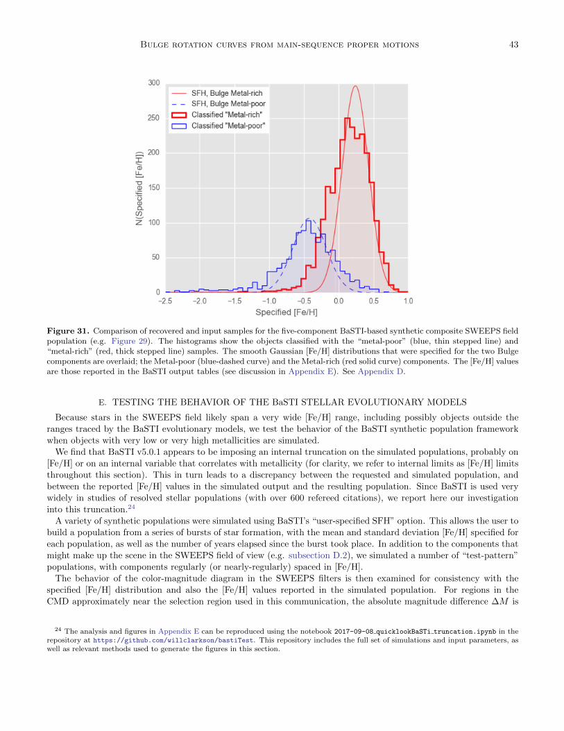
Bulge rotation curves from main-sequence proper motions 43

Figure 31. Comparison of recovered and input samples for the five-component BaSTI-based synthetic composite SWEEPS fieldpopulation (e.g. Figure 29). The histograms show the objects classified with the “metal-poor” (blue, thin stepped line) and“metal-rich” (red, thick stepped line) samples. The smooth Gaussian [Fe/H] distributions that were specified for the two Bulgecomponents are overlaid; the Metal-poor (blue-dashed curve) and the Metal-rich (red solid curve) components. The [Fe/H] valuesare those reported in the BaSTI output tables (see discussion in Appendix E). See Appendix D.

E. TESTING THE BEHAVIOR OF THE BaSTI STELLAR EVOLUTIONARY MODELS

Because stars in the SWEEPS field likely span a very wide [Fe/H] range, including possibly objects outside the

ranges traced by the BaSTI evolutionary models, we test the behavior of the BaSTI synthetic population framework

when objects with very low or very high metallicities are simulated.

We find that BaSTI v5.0.1 appears to be imposing an internal truncation on the simulated populations, probably on

[Fe/H] or on an internal variable that correlates with metallicity (for clarity, we refer to internal limits as [Fe/H] limits

throughout this section). This in turn leads to a discrepancy between the requested and simulated population, and

between the reported [Fe/H] values in the simulated output and the resulting population. Since BaSTI is used very

widely in studies of resolved stellar populations (with over 600 refereed citations), we report here our investigation

into this truncation.24

A variety of synthetic populations were simulated using BaSTI’s “user-specified SFH” option. This allows the user to

build a population from a series of bursts of star formation, with the mean and standard deviation [Fe/H] specified for

each population, as well as the number of years elapsed since the burst took place. In addition to the components that

might make up the scene in the SWEEPS field of view (e.g. subsection D.2), we simulated a number of “test-pattern”

populations, with components regularly (or nearly-regularly) spaced in [Fe/H].

The behavior of the color-magnitude diagram in the SWEEPS filters is then examined for consistency with the

specified [Fe/H] distribution and also the [Fe/H] values reported in the simulated population. For regions in the

CMD approximately near the selection region used in this communication, the absolute magnitude difference ∆M is

24 The analysis and figures in Appendix E can be reproduced using the notebook 2017-09-08 quicklookBaSTi truncation.ipynb in therepository at https://github.com/willclarkson/bastiTest. This repository includes the full set of simulations and input parameters, aswell as relevant methods used to generate the figures in this section.

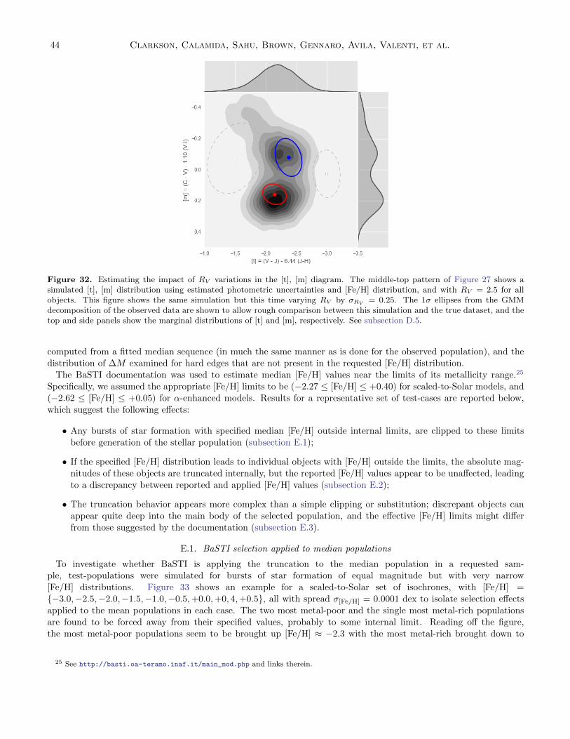
44 Clarkson, Calamida, Sahu, Brown, Gennaro, Avila, Valenti, et al.

Figure 32. Estimating the impact of RV variations in the [t], [m] diagram. The middle-top pattern of Figure 27 shows asimulated [t], [m] distribution using estimated photometric uncertainties and [Fe/H] distribution, and with RV = 2.5 for allobjects. This figure shows the same simulation but this time varying RV by σRV = 0.25. The 1σ ellipses from the GMMdecomposition of the observed data are shown to allow rough comparison between this simulation and the true dataset, and thetop and side panels show the marginal distributions of [t] and [m], respectively. See subsection D.5.

computed from a fitted median sequence (in much the same manner as is done for the observed population), and the

distribution of ∆M examined for hard edges that are not present in the requested [Fe/H] distribution.

The BaSTI documentation was used to estimate median [Fe/H] values near the limits of its metallicity range.25

Specifically, we assumed the appropriate [Fe/H] limits to be (−2.27 ≤ [Fe/H] ≤ +0.40) for scaled-to-Solar models, and

(−2.62 ≤ [Fe/H] ≤ +0.05) for α-enhanced models. Results for a representative set of test-cases are reported below,

which suggest the following effects:

• Any bursts of star formation with specified median [Fe/H] outside internal limits, are clipped to these limits

before generation of the stellar population (subsection E.1);

• If the specified [Fe/H] distribution leads to individual objects with [Fe/H] outside the limits, the absolute mag-

nitudes of these objects are truncated internally, but the reported [Fe/H] values appear to be unaffected, leading

to a discrepancy between reported and applied [Fe/H] values (subsection E.2);

• The truncation behavior appears more complex than a simple clipping or substitution; discrepant objects can

appear quite deep into the main body of the selected population, and the effective [Fe/H] limits might differ

from those suggested by the documentation (subsection E.3).

E.1. BaSTI selection applied to median populations

To investigate whether BaSTI is applying the truncation to the median population in a requested sam-

ple, test-populations were simulated for bursts of star formation of equal magnitude but with very narrow

[Fe/H] distributions. Figure 33 shows an example for a scaled-to-Solar set of isochrones, with [Fe/H] =

{−3.0,−2.5,−2.0,−1.5,−1.0,−0.5,+0.0,+0, 4,+0.5}, all with spread σ[Fe/H] = 0.0001 dex to isolate selection effects

applied to the mean populations in each case. The two most metal-poor and the single most metal-rich populations

are found to be forced away from their specified values, probably to some internal limit. Reading off the figure,

the most metal-poor populations seem to be brought up [Fe/H] ≈ −2.3 with the most metal-rich brought down to

25 See http://basti.oa-teramo.inaf.it/main_mod.php and links therein.

Bulge rotation curves from main-sequence proper motions 45

Figure 33. Testing the relationship between specified and simulated metallicities when bursts of star formation with a verywide range of median [Fe/H] values is requested with the BaSTI interface. Left top: specified and simulated [Fe/H] medianvalues. The green horizontal lines show the median [Fe/H] values for the bursts of star formation, with the gray points indicating[Fe/H] values reported in the output simulation. In this example, specified bursts are ordered from bottom to top and left toright in the simulated objects. Left bottom: absolute magnitude CMD in the SWEEPS filters of the resulting population, colorcoded by reported [Fe/H]. The black dots and line refer to the fitted fiducial in the selection region and a polynomial fit tothe fiducial, respectively. Right top: absolute magnitude offsets ∆M from the adopted fiducial, ordered by SWEEPS color,with symbols color-coded by [Fe/H] reported in the simulated population. Right bottom: histogram of ∆M . Here the specifiedmedian [Fe/H] values were {−3.0,−2.5,−2.0,−1.5,−1.0,−0.5,+0.0,+0, 4,+0.5}, all with specified spread σ[Fe/H] = 0.0001 dex.Populations with [Fe/H] . −2.3 or [Fe/H] & +0.4 seem to have been wrapped by BaSTI to the metallicity limits. Seesubsection E.1.

[Fe/H] ≈ +0.40. These values are entirely consistent with the [Fe/H] limits suggested by the BaSTI documentation

referenced earlier.

This suggests that BaSTI enforces [Fe/H] limits on the median populations requested in a simulation.

E.2. BaSTI truncation near the [Fe/H] limits

To investigate whether BaSTI applies a truncation to [Fe/H] values that are carried outside internal [Fe/H] limits due

to the specified population spread, test-populations were simulated including a single population well away from the lim-

its, and one component each just inside the two limits. Components were specified with [Fe/H] = {−2.5,−1.2,+0.05},all with specified spread σ[Fe/H] = 0.1 dex, to ensure that the two components near the [Fe/H] limits each include

substantial numbers of objects outside these limits, while the middle population has very few such objects.

Figure 34 shows the resulting simulation. Curiously, although the [Fe/H] values reported in the simulated populations

show no truncation, the CMD and the simulated absolute magnitudes quite clearly do show truncation, with a hard

edge at both the upper and lower [Fe/H] extrema.

46 Clarkson, Calamida, Sahu, Brown, Gennaro, Avila, Valenti, et al.

Figure 34. Testing the behavior of BaSTI simulations for populations with [Fe/H] close to the internal boundaries. Left column:panels and symbols as Figure 33, with specified bursts ordered bottom-top and their simulated populations ordered left-right.Here a three-component α-enhanced population is simulated, with [Fe/H] = {−2.5,−1.2,+0.05}, all with specified spreadσ[Fe/H] = 0.1 dex. The metal-poor and metal-rich populations show sharp cut-offs in both the CMD and the ∆M distribution,which are not present in either the central population (well away from the [Fe/H] limits), nor are the cutoffs present in thereported [Fe/H] distributions of the metal-poor and metal-rich populations. (Curvature in the metal-poor hard-edge is likely dueto differences in the shape of the median-population for [Fe/H] = −2.5 and that for [Fe/H] = −1.2.) The simulated magnitudesof the resulting populations show hard edges at the metal-rich and metal-poor ends, suggesting truncation in the deliveredpopulations. Curiously, however, there is no such truncation in the corresponding reported [Fe/H] values. This suggests that atruncation is being applied after the assignment of [Fe/H] values to simulated objects. See subsection E.2.

We therefore find that BaSTI does not truncate [Fe/H] values at the stage of assignment to simulated objects, and

these non-truncated [Fe/H] values are carried through to the output simulated population. However, a truncation is

applied at some stage before the absolute magnitudes are included in the simulated population. This results both

in a hard edge to the distribution of simulated absolute magnitudes, and also a discrepancy between the reported

[Fe/H] values and the absolute magnitudes, in the simulation output.

E.3. BaSTI truncation near the metal-rich limit

To chart the behavior of the truncation near the [Fe/H] limits in more detail, we simulated a single test population

near the metal-rich limit. Figure 35 shows the result for a scaled-to-Solar component with [Fe/H] = +0.24 and scatter

σ[Fe/H] = 0.19. In this case, the truncation appears to be quite dramatic, with a narrow, highly over-represented

component in the ∆M distribution.

However, the behaviour of the simulator near an [Fe/H] limit is not as straightforward as a simple substitution of

the [Fe/H] limit for all objects beyond it. Figure 30 shows a simulated metal-rich population partitioned by [Fe/H],

which allows us to distinguish objects that were assigned [Fe/H] values above the metal-rich limit (and thus would

be assumed to be truncated). Objects with outlier [Fe/H] values do not only appear at the location where absolute

Bulge rotation curves from main-sequence proper motions 47

Figure 35. Charting detailed behavior of BaSTI truncation near the metal-rich limit. Panels and symbols are as in Figure 34;here a single scaled-to-Solar component is simulated with [Fe/H] = +0.24 and scatter σ[Fe/H] = 0.19. A strong pile-up is observedat the bright end of the ∆M distribution (curvature in this component is likely due to systematics in the determination of thefiducial ridgeline, which was determined from the simulated CMD, as would be the case for observed populations, rather thanspecified using an isochrone). Again, while a strong truncation is observed in the simulated absolute magnitudes, no such hardedge is present in the reported [Fe/H] values. See subsection E.3 and Figure 30.

magnitudes pile up; a substantial fraction show magnitudes deeper into the main population (see the bottom-left panel

of Figure 30).

That the pile-up implying truncation is also observed at the metal-rich edge of the population with simulated

metallicities within the limits according to the BaSTI documentation, suggests that the effective metallicity limits

may differ from those documented; see the middle-left panel of Figure 30. (We have not yet dissected this simulated

population by binarity, which might offer another avenue for objects to wander into truncation territory.)

We therefore find that the internal truncation applied by BaSTI is not limited to a simple pegging of values to an

internal boundary. The behavior probably necessitates some sort of selection on ∆M to produce a cleaner unaffected

sample. We adopt one such approach in subsection D.3.

F. CROSS-CONTAMINATION IN THE [t], [m] DIAGRAM

We consider here the mixing of the “metal-rich” and “metal-poor” samples (and thus rotation curves) due to cross-

contamination in the [t], [m] space from which the two samples were drawn (subsection 5.2).

While the formal membership probability threshold wik ≥ 0.7 was chosen to be somewhat conservative, some amount

of sample contamination in [t], [m] is highly likely. Since the ([t], [m]) each represent flux ratios constructed from

photometry in three filters, it is likely that objects best characterized at one side of the abundance range for the bulge,

might be classified to an object in the other due to photometric uncertainty. In principle, a nearly-flat rotation curve

for one sample could be polluted by samples from another sample with a large-amplitude rotation curve, and vice

48 Clarkson, Calamida, Sahu, Brown, Gennaro, Avila, Valenti, et al.

Figure 36. Simple Monte Carlo test for cross-contamination of the “metal-rich” and “metal-poor” samples in ([t], [m]) space.Objects are simulated from the best-fit 4-component GMM in ([t], [m]) space (whose parameters are given in Table 5), perturbedby measurement uncertainty, and re-characterized using another 4-component GMM. The model component assigned to eachobject in the characterization is then compared to the component from which the object was drawn. The left column showsthe distribution of origin components for objects classified as “metal-poor” (top left, blue), the right column shows the origincomponents for objects classified as “metal-rich” (top right, red). In each column the top panel shows the distributions ofobjects classified correctly, the others show the distributions of objects classified with a different (indicated) component. Inboth columns, component “0” (blue) is the “metal-poor” component, component “3” (red) is the “metal-rich” component, andcomponents “1” & “2” (gray) are the remaining components, used to characterize the background in ([t], [m]). See Appendix F.

versa, sufficiently to weaken the trends in the high-amplitude sample while imprinting a signal on the other that is not

in fact present.

A rigorous exploration of the cross-contamination in ([t], [m]) requires a somewhat involved set of computations.

For example, flat priors in observed flux (for each the five filters used in BTS) are unlikely to translate into flat priors

in ([t], [m]) space, as suggested graphically by the degeneracy exhibited by very metal-poor populations in the ([t],

[m]) diagram (e.g. Brown et al. 2009). To properly account for cross-contamination likely requires simulations of

the underlying metallicity and temperature distributions (for which a range of shape parameters for the distributions

would also need exploration), then translating them forward into the probability density function in ([t], [m]) including

full accounting for the shape of the measurement uncertainty distributions and covariances in each of the filters. We

consider this beyond the scope of the present work.

Instead, we have performed a simpler quantitative estimate of the degree of cross-contamination in ([t], [m]) space.

We assume that the four-component Gaussian Mixture Model (GMM) is indeed a reasonable characterization of the

observed distribution of ([t], [m]) values, and also that the measurement uncertainties in this space can be described

as two-dimensional Gaussians for each object. Samples in ([t], [m]) are simulated by drawing from the best-fit 4-

component GMM and perturbing each object by an uncertainty covariance matrix (Equation A2) drawn randomly

without replacement from the observed population. Then a four-component GMM is fit to each sample, and objects

classified to belong to a model component using the wik ≥ 0.7 threshold that was used on the observed dataset

(an object cannot satisfy this condition for more than one model component by construction). Finally, the model

component classification for each object is compared to the model component from which it was originally drawn, to

measure the contamination for each component (i.e. the fraction of objects classified with component K but drawn

from k 6= K).

Figure 36 shows the results of 5,000 simulation sets. Generally, the “metal-poor” component is relatively uncontam-

inated by the “metal-rich” population (at < 1%), but is more strongly contaminated (at the ∼ 5% level) by broad

background component “2.” Under the assumptions of this simulation, the “metal-poor” sample suffers . 5.5% con-

tamination from the other components (see the left column of Figure 36).

Bulge rotation curves from main-sequence proper motions 49

The “metal-rich” component is more strongly contaminated. Roughly 5% of this sample is contaminated by the

“metal-poor” component, with the broad background component “2” contributing ∼ 3.5%. Under the simulation

assumptions, the “metal-rich” component suffers ∼ 8.5% contamination from the other components (see the right

column of Figure 36).

These ranges almost certainly underestimate the true contamination between samples in ([t], [m]). The observed

([t], [m]) distribution tends to be less centrally peaked than the model samples (Figure 5), suggesting the model

likely generates samples whose classification by [t], [m] is artificially less vulnerable to contamination than in reality.

Furthermore, even if the distribution in flux ratio due to measurement uncertainty is Gaussian for a given filter,

for uncertainties σ(∆F/F0) & 0.1 the apparent magnitude uncertainty distribution will deviate substantially from a

Gaussian.

Full exploration of these effects is deferred to future work. For the present, our limited simulation suggests that the

two samples are contaminated in ([t], [m]) at the ∼ 5%− 10% level, using the wik > 0.7 threshold for classification.

G. ROTATION CURVES AND BIN STATISTICS IN TABULAR FORM

Full characterization of the variation of the proper motion ellipse with photometric parallax for the two samples

can be found in Tables 11 and 13, while Tables 12 and 14 present the same results after converting from relative

photometric parallax and proper motion to distance and transverse velocity. The bin statistics for the fine-grained

binning scheme are presented in Table 15 and Table 16.

For ease of interpretation and to aid direct comparison with other work, we also tabulate the rotation curves and bin

statistics for a binning scheme with constant-width bins (in photometric parallax) for each sample; see Tables 17-22.

50 Clarkson, Calamida, Sahu, Brown, Gennaro, Avila, Valenti, et al.

Table

11

.O

bse

rved

rota

tion

tren

dfo

rth

e“m

etal-

rich

”sa

mple

,w

ith

unce

rtain

tyra

nges

giv

enas

1σ

lim

its

base

don

1000

para

met

ric

boots

trap

tria

ls.

See

dis

cuss

ion

insu

bse

ctio

n4.1

.

π′

Bin

edges

N〈µl〉

〈µb〉

aµ

bµ

φlb

a/b

σ2 ll

σ2 bb

Clb

mag

mag

(mas

yr−

1)

(mas

yr−

1)

(mas

yr−

1)

(mas

yr−

1)

(◦)

(mas2

yr−

2)

(mas2

yr−

2)

(mas2

yr−

2)

-1.3

4-1

.60,-

1.1

925

2.7

2±

0.4

99

−0.1

1±

0.2

56

2.5±

0.3

41.3±

0.1

7−

4.1±

8.1

11.9

8±

0.1

01

6.3

8±

1.7

40

1.6

5±

0.4

34

0.3

4±

0.5

94

-0.7

0-1

.18,-

0.5

2198

1.6

8±

0.1

87

−0.2

2±

0.1

56

2.8±

0.1

42.2±

0.1

120.9±

8.5

81.2

8±

0.0

53

7.3

3±

0.7

16

5.1

0±

0.5

06−

1.0

0±

0.4

43

-0.4

0-0

.52,-

0.3

4199

1.2

0±

0.1

93

−0.1

0±

0.1

74

2.9±

0.1

52.3±

0.1

228.5±

8.5

71.2

7±

0.0

55

7.5

2±

0.7

66

5.8

1±

0.6

09−

1.3

1±

0.4

62

-0.2

9-0

.34,-

0.2

4198

1.0

4±

0.1

88

−0.0

7±

0.1

83

2.8±

0.1

42.4±

0.1

250.7±

24.9

01.1

6±

0.0

56

7.0

9±

0.6

89

6.6

9±

0.7

12−

0.9

9±

0.5

00

-0.2

1-0

.24,-

0.1

7196

1.2

3±

0.1

84

−0.0

7±

0.1

95

2.9±

0.1

42.4±

0.1

251.7±

17.7

61.1

9±

0.0

57

7.3

4±

0.6

82

6.7

7±

0.7

56−

1.1

7±

0.5

22

-0.1

4-0

.17,-

0.1

1200

0.8

9±

0.2

02

0.0

1±

0.1

94

3.0±

0.1

52.5±

0.1

338.2±

15.3

11.1

9±

0.0

55

8.1

3±

0.8

34

7.4

9±

0.7

54−

1.3

3±

0.5

47

-0.0

9-0

.11,-

0.0

6199

0.8

9±

0.2

18

0.1

9±

0.2

00

3.3±

0.1

72.6±

0.1

331.7±

9.7

01.2

5±

0.0

55

9.6

0±

0.9

84

7.8

9±

0.8

23−

1.7

1±

0.6

26

-0.0

4-0

.06,-

0.0

1198

0.4

6±

0.2

21

0.1

2±

0.1

97

3.2±

0.1

62.5±

0.1

232.5±

8.6

71.2

7±

0.0

54

9.2

7±

0.9

14

7.5

9±

0.7

42−

1.8

0±

0.5

91

0.0

2-0

.01,

0.0

4198−

0.1

5±

0.2

15

0.2

7±

0.2

02

3.1±

0.1

52.7±

0.1

337.9±

20.3

01.1

5±

0.0

55

8.7

8±

0.8

51

8.2

1±

0.8

25−

1.1

3±

0.6

15

0.0

70.0

4,

0.0

9199−

0.0

1±

0.2

20

0.2

9±

0.1

93

3.2±

0.1

62.5±

0.1

332.2±

9.3

61.2

7±

0.0

53

9.3

0±

0.9

03

7.6

1±

0.7

87−

1.7

6±

0.6

04

0.1

20.0

9,

0.1

5199−

0.5

0±

0.2

01

0.3

2±

0.1

91

3.2±

0.1

62.3±

0.1

240.9±

6.6

71.3

7±

0.0

52

8.0

2±

0.8

10

7.3

5±

0.7

27−

2.3

1±

0.5

75

0.1

80.1

5,

0.2

1197−

0.8

1±

0.1

71

0.5

1±

0.1

84

2.7±

0.1

32.4±

0.1

160.1±

35.2

81.1

2±

0.0

54

6.9

6±

0.6

04

6.2

0±

0.7

17−

0.6

6±

0.4

67

0.2

50.2

1,

0.2

9200−

1.0

3±

0.1

77

0.2

6±

0.1

60

2.5±

0.1

22.2±

0.1

025.6±

18.4

31.1

4±

0.0

53

6.0

7±

0.5

95

5.1

4±

0.4

98−

0.5

8±

0.3

89

0.3

40.2

9,

0.4

2198−

1.1

3±

0.1

47−

0.0

1±

0.1

39

2.1±

0.1

01.9±

0.0

922.8±

20.1

91.1

3±

0.0

54

4.4

2±

0.4

46

3.7

0±

0.3

81−

0.3

7±

0.2

82

0.5

60.4

2,

1.4

3168−

1.0

3±

0.1

20

0.0

3±

0.1

30

1.7±

0.0

81.5±

0.0

774.2±

59.4

71.0

8±

0.0

53

2.7

3±

0.2

59

2.4

1±

0.3

03−

0.1

0±

0.1

99

Bulge rotation curves from main-sequence proper motions 51

Table

12

.A

sT

able

11

but

wit

hphoto

met

ric

para

llaxes

and

pro

per

moti

ons

conver

ted

into

dis

tance

sand

vel

oci

ties

usi

ng

are

fere

nce

dis

tance

of

7.7

6

kp

c.See

dis

cuss

ion

insu

bse

ctio

n4.1

.

ddlo,dhi

N〈vl〉

〈vb〉

av

bv

φlb

a/b

σ2 ll,v

σ2 bb,v

σ2 lb,v

kp

ckp

c(k

ms−

1)

(km

s−1)

(km

s−1)

(km

s−1)

(◦)

(km

2s−

2)

(km

2s−

2)

(km

2s−

2)

4.1

93.7

1,4

.49

25

54.1

7±

9.9

21

−2.1

1±

5.0

82

50±

6.9

25±

3.4

−4.1±

8.1

11.9

8±

0.1

01

126.8±

34.6

032.8±

8.6

36.8±

11.8

0

5.6

14.5

0,6

.12

198

44.8

0±

4.9

78

−5.9

6±

4.1

63

74±

3.6

58±

2.8

20.9±

8.5

81.2

8±

0.0

53

195.2±

19.0

5135.6±

13.4

8−

26.7±

11.7

9

6.4

76.1

2,6

.64

199

36.7

5±

5.9

26

−2.9

9±

5.3

33

88±

4.5

69±

3.5

28.5±

8.5

71.2

7±

0.0

55

230.6±

23.5

0178.1±

18.6

8−

40.3±

14.1

7

6.8

06.6

4,6

.95

198

33.6

8±

6.0

53

−2.3

1±

5.8

96

91±

4.4

78±

3.8

50.7±

24.9

01.1

6±

0.0

56

228.8±

22.2

2215.9±

22.9

6−

31.8±

16.1

2

7.0

56.9

5,7

.16

196

41.0

3±

6.1

58

−2.4

7±

6.5

04

96±

4.8

81±

4.0

51.7±

17.7

61.1

9±

0.0

57

245.2±

22.8

0226.4±

25.2

6−

39.2±

17.4

4

7.2

77.1

6,7

.36

200

30.8

1±

6.9

68

0.2

1±

6.7

03

104±

5.0

88±

4.3

38.2±

15.3

11.1

9±

0.0

55

280.4±

28.7

5258.3±

25.9

8−

45.9±

18.8

6

7.4

47.3

6,7

.53

199

31.5

6±

7.6

99

6.6

7±

7.0

52

115±

5.9

92±

4.6

31.7±

9.7

01.2

5±

0.0

55

338.7±

34.7

2278.3±

29.0

5−

60.3±

22.0

7

7.6

37.5

4,7

.74

198

16.6

7±

7.9

73

4.4

2±

7.1

17

117±

5.7

92±

4.5

32.5±

8.6

71.2

7±

0.0

54

335.0±

33.0

5274.4±

26.8

2−

65.0±

21.3

7

7.8

37.7

4,7

.92

198

−5.6

3±

7.9

87

9.8

9±

7.4

83

115±

5.5

100±

4.9

37.9±

20.3

01.1

5±

0.0

55

325.9±

31.5

9304.8±

30.6

1−

42.0±

22.8

2

8.0

17.9

2,8

.09

199

−0.3

6±

8.3

34

10.9

3±

7.3

26

122±

5.9

97±

4.8

32.2±

9.3

61.2

7±

0.0

53

353.0±

34.2

8288.9±

29.8

9−

66.8±

22.9

5

8.2

08.1

0,8

.30

199−

19.3

6±

7.7

92

12.6

1±

7.4

17

123±

6.2

90±

4.5

40.9±

6.6

71.3

7±

0.0

52

311.5±

31.4

7285.4±

28.2

6−

89.6±

22.3

3

8.4

28.3

0,8

.54

197−

32.2

4±

6.8

07

20.3

9±

7.3

29

108±

5.2

96±

4.5

60.1±

35.2

81.1

2±

0.0

54

277.8±

24.1

0247.2±

28.6

1−

26.2±

18.6

2

8.7

08.5

4,8

.88

200−

42.4

8±

7.2

89

10.7

6±

6.5

95

104±

4.8

91±

4.2

25.6±

18.4

31.1

4±

0.0

53

250.4±

24.5

3212.0±

20.5

5−

23.9±

16.0

4

9.0

78.8

8,9

.40

198−

48.7

1±

6.3

29−

0.4

5±

5.9

69

92±

4.3

81±

3.9

22.8±

20.1

91.1

3±

0.0

54

190.0±

19.1

6159.2±

16.3

8−

15.7±

12.1

5

10.0

29.4

0,1

4.9

9168−

48.9

6±

5.6

81

1.4

9±

6.1

54

79±

3.9

73±

3.6

74.2±

59.4

71.0

8±

0.0

53

129.8±

12.3

0114.4±

14.3

8−

4.7±

9.4

6

52 Clarkson, Calamida, Sahu, Brown, Gennaro, Avila, Valenti, et al.

Table

13

.O

bse

rved

rota

tion

tren

dfo

rth

e“m

etal-

poor”

sam

ple

,w

ith

unce

rtain

tyra

nges

giv

enas

1σ

lim

its

base

don

1000

para

met

ric

boots

trap

tria

ls.

See

dis

cuss

ion

insu

bse

ctio

n4.1

.

π′

Bin

edges

N〈µl〉

〈µb〉

aµ

bµ

φlb

a/b

σ2 ll

σ2 bb

Clb

mag

mag

(mas

yr−

1)

(mas

yr−

1)

(mas

yr−

1)

(mas

yr−

1)

(◦)

(mas2

yr−

2)

(mas2

yr−

2)

(mas2

yr−

2)

-1.7

2-2

.02,-

1.5

724

3.0

0±

0.5

42

0.0

8±

0.4

13

2.7±

0.3

71.9±

0.2

6−

18.4±

20.3

71.4

5±

0.1

26

6.9

8±

1.9

73

3.8

9±

1.1

01

1.1

6±

1.0

48

-1.3

7-1

.53,-

1.3

125

2.4

5±

0.5

01

−0.6

0±

0.5

61

2.8±

0.3

42.4±

0.2

969.8±

56.9

11.1

5±

0.1

13

7.6

4±

1.6

30

6.1

9±

2.1

00−

0.6

2±

1.3

52

-1.0

4-1

.30,-

0.8

3199

0.5

5±

0.2

33

0.1

2±

0.2

05

3.3±

0.1

62.8±

0.1

314.7±

12.9

81.2

0±

0.0

54

10.9

5±

1.0

70

7.9

3±

0.7

89−

0.8

5±

0.6

79

-0.7

1-0

.83,-

0.6

2198

0.4

8±

0.2

27

−0.1

2±

0.1

96

3.4±

0.1

72.6±

0.1

326.9±

7.1

01.3

3±

0.0

51

10.7

2±

1.0

96

7.6

7±

0.7

66−

2.0

8±

0.6

51

-0.5

3-0

.62,-

0.4

7199

0.6

1±

0.2

28

−0.1

1±

0.2

19

3.5±

0.1

72.6±

0.1

345.3±

7.8

31.3

2±

0.0

52

9.5

4±

0.9

69

9.4

9±

0.9

68−

2.5

5±

0.6

99

-0.4

0-0

.47,-

0.3

6198

0.2

7±

0.2

11

−0.1

0±

0.2

16

3.3±

0.1

62.6±

0.1

346.7±

8.9

51.2

6±

0.0

54

9.1

5±

0.8

69

8.9

1±

0.8

96−

2.0

7±

0.6

43

-0.3

1-0

.35,-

0.2

7199

0.2

1±

0.2

33

−0.0

3±

0.2

08

3.2±

0.1

52.9±

0.1

3−

0.3±

21.7

01.1

2±

0.0

54

10.4

7±

1.0

52

8.3

9±

0.8

31

0.0

1±

0.6

62

-0.2

3-0

.27,-

0.1

9199

0.0

2±

0.2

23

0.5

8±

0.2

14

3.2±

0.1

52.8±

0.1

442.5±

22.8

21.1

3±

0.0

56

9.1

0±

0.9

41

8.9

0±

0.8

88−

1.1

1±

0.6

62

-0.1

6-0

.19,-

0.1

3197

0.0

4±

0.2

15

0.0

1±

0.2

18

3.3±

0.1

62.8±

0.1

347.7±

18.5

91.1

7±

0.0

54

9.3

1±

0.8

94

9.0

5±

0.9

45−

1.4

1±

0.6

48

-0.0

9-0

.13,-

0.0

5198−

0.0

3±

0.2

12

0.1

8±

0.2

10

3.1±

0.1

32.9±

0.1

337.2±

42.4

51.0

6±

0.0

46

9.0

3±

0.8

59

8.7

7±

0.8

86−

0.4

6±

0.6

28

-0.0

1-0

.05,

0.0

2199−

0.2

1±

0.2

18

0.1

9±

0.1

89

3.0±

0.1

52.6±

0.1

21.5±

15.7

81.1

6±

0.0

56

8.9

3±

0.9

06

6.6

1±

0.6

56−

0.0

6±

0.5

48

0.0

50.0

2,

0.0

9199−

0.3

3±

0.2

03

0.3

1±

0.2

11

3.0±

0.1

32.7±

0.1

241.2±

33.6

71.0

9±

0.0

50

8.2

8±

0.8

37

8.1

0±

0.8

06−

0.6

9±

0.5

67

0.1

20.0

9,

0.1

6199−

0.2

7±

0.2

04−

0.0

4±

0.2

03

3.0±

0.1

42.7±

0.1

226.8±

25.5

11.1

1±

0.0

52

8.4

3±

0.8

58

7.4

4±

0.7

37−

0.6

7±

0.5

55

0.2

00.1

6,

0.2

5197−

0.5

8±

0.2

17

0.2

4±

0.2

09

3.0±

0.1

32.9±

0.1

3−

47.2±

47.6

81.0

5±

0.0

45

8.6

7±

0.8

71

8.6

2±

0.8

74

0.3

8±

0.6

14

0.3

00.2

5,

0.3

6199−

0.5

8±

0.1

80

0.4

2±

0.1

76

2.6±

0.1

22.4±

0.1

141.9±

30.3

31.1

0±

0.0

51

6.4

1±

0.6

23

6.2

8±

0.6

10−

0.6

1±

0.4

48

0.4

30.3

6,

0.5

0196−

0.7

3±

0.1

79

0.2

4±

0.1

62

2.5±

0.1

32.2±

0.1

117.3±

20.3

61.1

4±

0.0

57

6.2

9±

0.6

54

5.0

6±

0.5

09−

0.4

3±

0.4

22

0.6

30.5

0,

0.8

0192−

0.5

8±

0.1

43

0.1

5±

0.1

45

2.0±

0.0

91.9±

0.0

9−

67.9±

56.3

81.0

3±

0.0

44

3.9

9±

0.3

90

3.8

1±

0.3

94

0.0

8±

0.2

79

0.9

70.8

0,

1.4

5105−

0.2

1±

0.1

36

0.3

7±

0.1

23

1.3±

0.0

81.2±

0.0

84.5±

31.0

31.1

1±

0.0

64

1.8

1±

0.2

45

1.4

7±

0.2

02−

0.0

3±

0.1

53

Bulge rotation curves from main-sequence proper motions 53

Table

14

.A

sT

able

13

but

wit

hphoto

met

ric

para

llaxes

and

pro

per

moti

ons

conver

ted

into

dis

tance

sand

vel

oci

ties

usi

ng

are

fere

nce

dis

tance

of

7.7

6kp

c.

See

dis

cuss

ion

insu

bse

ctio

n4.1

.

ddlo,dhi

N〈vl〉

〈vb〉

av

bv

φlb

a/b

σ2 ll,v

σ2 bb,v

σ2 lb,v

kp

ckp

c(k

ms−

1)

(km

s−1)

(km

s−1)

(km

s−1)

(◦)

(km

2s−

2)

(km

2s−

2)

(km

2s−

2)

3.5

23.0

7,3

.77

24

50.0

8±

9.0

46

1.3

7±

6.9

00

45±

6.2

31±

4.3

−18.4±

20.3

71.4

5±

0.1

26

116.5±

32.9

465.0±

18.3

819.3±

17.5

0

4.1

43.8

3,4

.25

25

48.0

8±

9.8

27

−11.7

9±

11.0

02

55±

6.7

48±

5.7

69.8±

56.9

11.1

5±

0.1

13

149.9±

31.9

7121.4±

41.1

9−

12.1±

26.5

3

4.8

04.2

6,5

.30

199

12.5

9±

5.3

03

2.8

3±

4.6

67

76±

3.6

63±

3.0

14.7±

12.9

81.2

0±

0.0

54

249.3±

24.3

6180.7±

17.9

7−

19.4±

15.4

7

5.6

05.3

0,5

.84

198

12.8

7±

6.0

39

−3.0

7±

5.2

04

91±

4.6

68±

3.4

26.9±

7.1

01.3

3±

0.0

51

284.7±

29.1

0203.8±

20.3

5−

55.2±

17.2

8

6.0

75.8

4,6

.26

199

17.5

2±

6.5

55

−3.1

4±

6.2

86

100±

5.0

76±

3.7

45.3±

7.8

31.3

2±

0.0

52

274.4±

27.8

6272.7±

27.8

4−

73.2±

20.1

0

6.4

56.2

6,6

.59

198

8.3

6±

6.4

49

−2.9

7±

6.6

09

102±

5.0

81±

3.9

46.7±

8.9

51.2

6±

0.0

54

279.6±

26.5

6272.2±

27.3

7−

63.3±

19.6

4

6.7

16.5

9,6

.85

199

6.6

7±

7.4

12

−1.0

1±

6.6

25

103±

4.9

92±

4.3

−0.3±

21.7

01.1

2±

0.0

54

333.2±

33.4

7266.9±

26.4

40.4±

21.0

6

6.9

76.8

5,7

.09

199

0.5

3±

7.3

74

19.1

9±

7.0

61

105±

5.1

93±

4.5

42.5±

22.8

21.1

3±

0.0

56

300.6±

31.0

9294.0±

29.3

2−

36.7±

21.8

5

7.2

07.1

0,7

.32

197

1.1

9±

7.3

55

0.4

8±

7.4

35

111±

5.3

95±

4.6

47.7±

18.5

91.1

7±

0.0

54

318.0±

30.5

3309.0±

32.2

6−

48.0±

22.1

2

7.4

47.3

2,7

.59

198

−1.1

5±

7.4

80

6.3

2±

7.4

16

108±

4.4

102±

4.7

37.2±

42.4

51.0

6±

0.0

46

318.5±

30.2

9309.3±

31.2

6−

16.3±

22.1

6

7.7

17.5

9,7

.82

199

−7.6

0±

7.9

52

6.9

1±

6.9

19

109±

5.3

94±

4.5

1.5±

15.7

81.1

6±

0.0

56

326.3±

33.1

1241.5±

23.9

7−

2.3±

20.0

2

7.9

57.8

2,8

.08

199−

12.4

2±

7.6

56

11.6

2±

7.9

62

112±

5.0

103±

4.7

41.2±

33.6

71.0

9±

0.0

50

312.3±

31.5

5305.4±

30.3

9−

25.9±

21.3

6

8.2

08.0

8,8

.35

199−

10.6

7±

7.9

19

−1.6

1±

7.8

78

115±

5.3

104±

4.7

26.8±

25.5

11.1

1±

0.0

52

327.8±

33.3

7289.3±

28.6

5−

26.2±

21.5

9

8.5

18.3

5,8

.69

197−

23.2

2±

8.7

62

9.5

1±

8.4

11

121±

5.2

116±

5.1

−47.2±

47.6

81.0

5±

0.0

45

349.7±

35.1

0347.4±

35.2

215.3±

24.7

4

8.8

98.6

9,9

.16

199−

24.3

6±

7.6

00

17.9

0±

7.4

32

111±

5.0

101±

4.5

41.9±

30.3

31.1

0±

0.0

51

270.3±

26.2

4264.8±

25.7

3−

25.6±

18.8

9

9.4

59.1

7,9

.75

196−

32.7

9±

8.0

16

10.8

6±

7.2

81

114±

5.6

99±

4.8

17.3±

20.3

61.1

4±

0.0

57

281.9±

29.2

9226.8±

22.8

2−

19.0±

18.9

2

10.3

79.7

6,1

1.2

1192−

28.6

3±

7.0

42

7.5

3±

7.1

52

99±

4.2

96±

4.3

−67.9±

56.3

81.0

3±

0.0

44

196.0±

19.1

8187.5±

19.3

64.2±

13.7

1

12.1

511.2

2,1

5.1

5105−

12.3

0±

7.8

46

21.1

5±

7.0

72

77±

4.7

70±

4.4

4.5±

31.0

31.1

1±

0.0

64

104.0±

14.1

084.8±

11.6

4−

1.5±

8.8

3

54 Clarkson, Calamida, Sahu, Brown, Gennaro, Avila, Valenti, et al.

Table 15. Bin statistics for the rotation curves of the “metal-rich” sample. Wedge volumesV and densities ρ assume the reference sample lies at distance 7.76 kpc. N(µl) and ρ(µl) denotethe counts and number densities of objects that would pass a kinematic cut of µl < −2.0 masyr−1. The binning scheme is the same as Table 11. The uncertainties quoted refer to 1σ rangesfrom 1000 parameteric bootstrap trials. See subsection 5.4.

π′ π′hi − π′lo d dhi − dlo N V ρ N(µl) f(µl) ρ(µl)

mag mag kpc kpc (pc3) (pc−3) (pc−3)

-1.34 0.415 4.19 0.782 25 1523.9 0.016 1± 0.9 0.04± 0.034 0.001± 0.0006

-0.70 0.664 5.61 1.611 198 5198.6 0.038 19± 3.7 0.10± 0.019 0.004± 0.0007

-0.40 0.179 6.47 0.525 199 2420.2 0.082 22± 4.6 0.11± 0.023 0.009± 0.0019

-0.29 0.097 6.80 0.303 198 1588.7 0.125 29± 4.7 0.15± 0.024 0.018± 0.0029

-0.21 0.066 7.05 0.214 196 1214.5 0.161 20± 4.4 0.10± 0.023 0.016± 0.0036

-0.14 0.059 7.27 0.197 200 1173.6 0.170 33± 5.2 0.17± 0.026 0.028± 0.0044

-0.09 0.051 7.44 0.175 199 1098.9 0.181 36± 5.4 0.18± 0.027 0.033± 0.0049

-0.04 0.058 7.63 0.204 198 1350.3 0.147 45± 5.6 0.23± 0.028 0.033± 0.0041

0.02 0.049 7.83 0.177 198 1228.2 0.161 54± 6.2 0.27± 0.031 0.044± 0.0050

0.07 0.048 8.01 0.177 199 1294.1 0.154 58± 6.2 0.29± 0.031 0.045± 0.0048

0.12 0.054 8.20 0.205 199 1556.7 0.128 60± 6.5 0.30± 0.033 0.039± 0.0042

0.18 0.062 8.42 0.241 197 1937.4 0.102 61± 6.4 0.31± 0.032 0.031± 0.0033

0.25 0.083 8.70 0.335 200 2878.9 0.069 73± 6.7 0.36± 0.033 0.025± 0.0023

0.34 0.123 9.07 0.519 198 4990.1 0.040 75± 6.5 0.38± 0.033 0.015± 0.0013

0.56 1.012 10.02 5.582 168 105291.0 0.002 43± 5.7 0.26± 0.034 0.000± 0.0001

Table 16. As Table 15 but for the “metal-poor” sample. See subsection 5.4.

π′ π′hi − π′lo d dhi − dlo N V ρ N(µl) f(µl) ρ(µl)

mag mag kpc kpc (pc3) (pc−3) (pc−3)

-1.72 0.450 3.52 0.706 24 1038.4 0.023 1± 0.8 0.04± 0.035 0.001± 0.0008

-1.37 0.225 4.14 0.418 25 783.9 0.032 2± 0.9 0.08± 0.037 0.003± 0.0012

-1.04 0.475 4.80 1.042 199 2701.7 0.074 39± 5.8 0.20± 0.029 0.014± 0.0022

-0.71 0.211 5.60 0.541 198 1914.0 0.103 50± 5.6 0.25± 0.028 0.026± 0.0029

-0.53 0.148 6.07 0.413 199 1740.3 0.114 36± 5.9 0.18± 0.030 0.021± 0.0034

-0.40 0.110 6.45 0.327 198 1542.5 0.128 49± 5.7 0.25± 0.029 0.032± 0.0037

-0.31 0.082 6.71 0.254 199 1310.3 0.152 54± 6.0 0.27± 0.030 0.041± 0.0046

-0.23 0.077 6.97 0.247 199 1364.6 0.146 50± 6.4 0.25± 0.032 0.037± 0.0047

-0.16 0.066 7.20 0.219 197 1295.1 0.152 56± 6.0 0.28± 0.031 0.043± 0.0047

-0.09 0.079 7.44 0.269 198 1702.3 0.116 49± 6.0 0.25± 0.030 0.029± 0.0035

-0.01 0.066 7.71 0.236 199 1587.5 0.125 52± 6.4 0.26± 0.032 0.033± 0.0040

0.05 0.070 7.95 0.257 199 1839.3 0.108 59± 6.4 0.30± 0.032 0.032± 0.0035

0.12 0.072 8.20 0.272 199 2096.1 0.095 65± 6.5 0.33± 0.033 0.031± 0.0031

0.20 0.086 8.51 0.338 197 2782.7 0.071 59± 6.7 0.30± 0.034 0.021± 0.0024

0.30 0.114 8.89 0.470 199 4291.1 0.046 59± 6.6 0.30± 0.033 0.014± 0.0015

0.43 0.134 9.45 0.586 196 6000.0 0.033 60± 6.2 0.31± 0.032 0.010± 0.0010

0.63 0.301 10.37 1.449 192 18176.3 0.011 42± 5.8 0.22± 0.030 0.002± 0.0003

0.97 0.652 12.15 3.929 105 87265.7 0.001 7± 3.0 0.07± 0.028 0.000± 0.0000

Bulge rotation curves from main-sequence proper motions 55

Table

17

.O

bse

rved

rota

tion

tren

dfo

rth

e“m

etal-

rich

”sa

mple

,usi

ng

aco

nst

ant-

wid

thbin

nin

gsc

hem

eand

wit

hunce

rtain

tyra

nges

giv

enas

1σ

lim

its

base

don

1000

para

met

ric

boots

trap

tria

ls.

See

dis

cuss

ion

insu

bse

ctio

n4.1

.

π′

Bin

edges

N〈µl〉

〈µb〉

aµ

bµ

φlb

a/b

σ2 ll

σ2 bb

Clb

mag

mag

(mas

yr−

1)

(mas

yr−

1)

(mas

yr−

1)

(mas

yr−

1)

(◦)

(mas2

yr−

2)

(mas2

yr−

2)

(mas2

yr−

2)

-0.8

2-0

.86,-

0.7

826

2.0

5±

0.5

43

−1.4

2±

0.3

41

2.8±

0.3

81.7±

0.2

36.5±

14.0

81.6

3±

0.1

16

8.0

3±

2.1

61

3.1

2±

0.8

07−

0.5

7±

0.9

96

-0.7

3-0

.77,-

0.6

931

0.1

8±

0.4

65

0.5

4±

0.4

49

3.0±

0.3

72.0±

0.2

540.6±

16.9

51.5

2±

0.1

14

6.7

3±

1.7

25

5.9

5±

1.4

69−

2.4

8±

1.1

84

-0.6

5-0

.69,-

0.6

038

1.6

4±

0.4

47

0.1

8±

0.3

37

2.8±

0.3

12.0±

0.2

213.4±

18.6

71.3

9±

0.1

03

7.8

1±

1.7

77

4.3

7±

1.0

19−

0.8

7±

0.9

32

-0.5

5-0

.60,-

0.5

158

1.6

7±

0.3

56

−0.1

9±

0.3

05

2.8±

0.2

32.3±

0.1

9−

18.0±

25.2

01.2

1±

0.0

91

7.3

6±

1.3

26

5.4

4±

0.9

94

0.6

9±

0.8

21

-0.4

6-0

.51,-

0.4

363

1.5

5±

0.3

20

−0.0

5±

0.3

24

2.7±

0.2

12.3±

0.1

937.3±

36.9

21.1

4±

0.0

79

6.5

2±

1.1

58

6.0

9±

1.1

41−

0.7

8±

0.7

74

-0.3

8-0

.42,-

0.3

4133

1.0

7±

0.2

47

−0.1

6±

0.2

13

3.0±

0.1

82.2±

0.1

327.4±

8.9

51.3

3±

0.0

64

7.9

4±

0.9

62

5.7

4±

0.6

90−

1.5

5±

0.5

90

-0.2

9-0

.34,-

0.2

5172

1.0

0±

0.1

94

−0.0

5±

0.2

07

2.8±

0.1

42.5±

0.1

252.4±

33.5

71.1

2±

0.0

56

7.0

1±

0.7

12

6.6

0±

0.7

53−

0.7

7±

0.5

26

-0.2

1-0

.25,-

0.1

6260

1.2

2±

0.1

56

−0.0

6±

0.1

63

2.9±

0.1

22.4±

0.1

054.8±

12.0

81.2

1±

0.0

48

7.3

3±

0.5

52

6.4

7±

0.6

36−

1.2

1±

0.4

26

-0.1

2-0

.16,-

0.0

8315

0.9

4±

0.1

73

0.1

4±

0.1

60

3.2±

0.1

32.6±

0.1

029.5±

8.4

51.2

3±

0.0

44

9.5

5±

0.7

74

7.7

5±

0.6

29−

1.5

0±

0.4

77

-0.0

3-0

.07,

0.0

1316

0.3

9±

0.1

79

0.1

3±

0.1

56

3.2±

0.1

32.6±

0.1

034.2±

7.8

71.2

4±

0.0

43

9.1

9±

0.7

37

7.8

6±

0.6

34−

1.6

8±

0.4

79

0.0

60.0

1,

0.1

0358−

0.2

1±

0.1

56

0.3

7±

0.1

45

3.1±

0.1

12.6±

0.1

036.0±

8.5

31.2

0±

0.0

43

8.4

5±

0.6

07

7.5

5±

0.5

68−

1.3

8±

0.4

32

0.1

40.1

0,

0.1

9297−

0.5

6±

0.1

70

0.2

7±

0.1

59

3.1±

0.1

22.4±

0.1

040.3±

7.1

61.2

7±

0.0

43

7.8

6±

0.6

43

7.2

8±

0.5

99−

1.7

4±

0.4

36

0.2

30.1

9,

0.2

7234−

0.9

7±

0.1

60

0.2

9±

0.1

56

2.5±

0.1

12.2±

0.1

034.2±

17.3

51.1

5±

0.0

52

5.9

0±

0.5

61

5.3

2±

0.4

76−

0.7

3±

0.3

75

0.3

10.2

8,

0.3

6164−

1.1

3±

0.1

56

0.2

1±

0.1

65

2.2±

0.1

12.0±

0.1

058.1±

44.4

41.1

0±

0.0

57

4.4

8±

0.4

67

4.1

1±

0.4

96−

0.3

7±

0.3

30

0.4

00.3

6,

0.4

592

−1.1

5±

0.2

34−

0.3

0±

0.2

09

2.2±

0.1

52.0±

0.1

37.0±

29.6

91.1

3±

0.0

69

4.9

5±

0.7

17

3.9

3±

0.5

78−

0.1

3±

0.4

59

0.4

90.4

5,

0.5

452

−0.9

9±

0.2

64

0.4

1±

0.2

72

2.0±

0.1

71.8±

0.1

5−

58.2±

50.0

21.1

2±

0.0

83

3.7

2±

0.6

50

3.3

6±

0.7

00

0.3

6±

0.5

02

0.5

60.5

4,

0.6

231

−0.8

0±

0.3

17

0.3

8±

0.2

67

1.7±

0.1

91.5±

0.1

6−

19.9±

37.9

01.1

6±

0.1

03

2.8

9±

0.7

24

2.3

1±

0.5

65

0.2

4±

0.4

34

0.6

70.6

3,

0.7

122

−1.3

8±

0.3

34−

0.2

5±

0.3

66

2.1±

0.3

11.2±

0.1

751.0±

16.8

71.7

7±

0.1

17

3.1

3±

0.7

67

2.5

2±

0.9

24−

1.4

3±

0.6

68

56 Clarkson, Calamida, Sahu, Brown, Gennaro, Avila, Valenti, et al.

Table

18

.A

sT

able

17

(i.e

.,usi

ng

aco

nst

ant-

wid

thbin

nin

gsc

hem

e)but

wit

hphoto

met

ric

para

llaxes

and

pro

per

moti

ons

conver

ted

into

dis

tance

sand

vel

oci

ties

usi

ng

are

fere

nce

dis

tance

of

7.7

6kp

c.See

dis

cuss

ion

insu

bse

ctio

n4.1

.

ddlo,dhi

N〈vl〉

〈vb〉

av

bv

φlb

a/b

σ2 ll,v

σ2 bb,v

σ2 lb,v

kp

ckp

c(k

ms−

1)

(km

s−1)

(km

s−1)

(km

s−1)

(◦)

(km

2s−

2)

(km

2s−

2)

(km

2s−

2)

5.3

35.2

2,5

.43

26

51.7

3±

13.7

19

−35.8

9±

8.6

24

72±

9.5

44±

5.8

6.5±

14.0

81.6

3±

0.1

16

202.7±

54.5

878.9±

20.3

9−

14.3±

25.1

6

5.5

35.4

3,5

.65

31

4.6

1±

12.1

94

14.1

6±

11.7

70

78±

9.8

51±

6.6

40.6±

16.9

51.5

2±

0.1

14

176.4±

45.2

4156.1±

38.5

2−

65.0±

31.0

6

5.7

55.6

6,5

.88

38

44.6

5±

12.1

92

4.9

1±

9.1

98

77±

8.4

56±

6.0

13.4±

18.6

71.3

9±

0.1

03

212.9±

48.4

3119.2±

27.7

8−

23.7±

25.4

0

6.0

25.8

9,6

.12

58

47.6

6±

10.1

46

−5.4

0±

8.7

11

79±

6.7

65±

5.5

−18.0±

25.2

01.2

1±

0.0

91

209.8±

37.8

4155.3±

28.3

719.8±

23.4

3

6.2

76.1

3,6

.37

63

46.0

1±

9.5

32

−1.3

9±

9.6

23

79±

6.2

70±

5.7

37.3±

36.9

21.1

4±

0.0

79

193.9±

34.4

5181.2±

33.9

5−

23.1±

23.0

1

6.5

36.3

8,6

.64

133

33.1

6±

7.6

49

−4.8

9±

6.5

77

91±

5.4

69±

4.1

27.4±

8.9

51.3

3±

0.0

64

245.6±

29.7

7177.7±

21.3

5−

48.1±

18.2

5

6.7

96.6

4,6

.92

172

32.1

7±

6.2

43

−1.5

5±

6.6

43

89±

4.4

79±

3.9

52.4±

33.5

71.1

2±

0.0

56

225.4±

22.9

1212.3±

24.2

2−

24.6±

16.9

3

7.0

56.9

2,7

.20

260

40.7

2±

5.2

30

−2.0

0±

5.4

62

96±

4.0

79±

3.3

54.8±

12.0

81.2

1±

0.0

48

245.1±

18.4

7216.2±

21.2

6−

40.6±

14.2

4

7.3

67.2

0,7

.50

315

32.9

5±

6.0

35

4.7

1±

5.5

66

112±

4.4

92±

3.6

29.5±

8.4

51.2

3±

0.0

44

333.1±

26.9

9270.3±

21.9

5−

52.2±

16.6

4

7.6

57.5

0,7

.80

316

13.9

6±

6.4

81

4.8

3±

5.6

56

117±

4.6

94±

3.6

34.2±

7.8

71.2

4±

0.0

43

333.1±

26.7

2284.9±

22.9

9−

60.9±

17.3

6

7.9

77.8

0,8

.12

358

−8.0

9±

5.8

94

13.9

3±

5.4

94

116±

4.2

97±

3.6

36.0±

8.5

31.2

0±

0.0

43

319.0±

22.9

1285.1±

21.4

4−

52.0±

16.3

1

8.2

98.1

3,8

.46

297

−21.9

8±

6.6

89

10.4

7±

6.2

57

120±

4.8

95±

3.8

40.3±

7.1

61.2

7±

0.0

43

308.7±

25.2

6286.0±

23.5

4−

68.5±

17.1

2

8.6

18.4

6,8

.81

234

−39.4

3±

6.5

48

11.8

9±

6.3

62

103±

4.7

90±

4.0

34.2±

17.3

51.1

5±

0.0

52

240.8±

22.9

1217.3±

19.4

2−

29.7±

15.3

3

8.9

78.8

1,9

.17

164

−48.0

8±

6.6

17

8.7

3±

7.0

30

92±

4.6

84±

4.3

58.1±

44.4

41.1

0±

0.0

57

190.2±

19.8

4174.6±

21.0

6−

15.9±

14.0

2

9.3

49.1

7,9

.54

92

−50.7

0±

10.3

61

−13.2

7±

9.2

48

99±

6.5

88±

5.9

7.0±

29.6

91.1

3±

0.0

69

219.4±

31.7

6173.8±

25.6

1−

5.7±

20.3

2

9.7

29.5

5,9

.93

52

−45.5

4±

12.1

47

19.0

4±

12.5

50

91±

7.7

82±

7.0

−58.2±

50.0

21.1

2±

0.0

83

171.3±

29.9

4154.8±

32.2

716.5±

23.1

3

10.0

69.9

4,1

0.3

331

−38.3

8±

15.1

28

17.8

9±

12.7

57

82±

9.1

71±

7.4

−19.9±

37.9

01.1

6±

0.1

03

137.6±

34.5

1110.4±

26.9

511.4±

20.6

8

10.5

510.3

5,1

0.7

722

−69.2

0±

16.6

90−

12.4

2±

18.3

08

103±

15.3

58±

8.6

51.0±

16.8

71.7

7±

0.1

17

156.4±

38.3

4126.1±

46.2

3−

71.4±

33.3

9

Bulge rotation curves from main-sequence proper motions 57

Table

19

.O

bse

rved

rota

tion

tren

dfo

rth

e“m

etal-

poor”

sam

ple

,usi

ng

aco

nst

ant-

wid

thbin

nin

gsc

hem

e,w

ith

unce

rtain

tyra

nges

giv

enas

1σ

lim

its

base

d

on

1000

para

met

ric

boots

trap

tria

ls.

See

dis

cuss

ion

insu

bse

ctio

n4.1

.

π′

Bin

edges

N〈µl〉

〈µb〉

aµ

bµ

φlb

a/b

σ2 ll

σ2 bb

Clb

mag

mag

(mas

yr−

1)

(mas

yr−

1)

(mas

yr−

1)

(mas

yr−

1)

(◦)

(mas2

yr−

2)

(mas2

yr−

2)

(mas2

yr−

2)

-1.2

4-1

.29,-

1.2

127

1.2

6±

0.6

39

0.8

9±

0.4

71

3.2±

0.3

82.4±

0.3

00.3±

24.7

61.3

3±

0.1

13

10.1

5±

2.6

02

5.7

8±

1.5

05

−0.0

2±

1.4

36

-1.1

6-1

.21,-

1.1

325

1.7

2±

0.6

45

−0.8

6±

0.6

29

3.7±

0.4

92.8±

0.3

740.4±

29.0

21.3

2±

0.1

22

11.2

7±

2.9

67

10.3

2±

2.9

25−

2.9

1±

2.2

34

-1.0

7-1

.12,-

1.0

447

−0.0

9±

0.5

18

0.0

4±

0.4

21

3.5±

0.3

32.8±

0.2

75.0±

27.4

61.2

1±

0.0

95

11.9

1±

2.4

29

8.1

3±

1.6

94

−0.3

3±

1.4

34

-0.9

9-1

.04,-

0.9

533

0.9

4±

0.5

79

0.5

4±

0.4

57

3.4±

0.4

02.5±

0.3

04.9±

20.2

71.3

6±

0.1

14

11.6

6±

2.8

10

6.3

2±

1.5

80

−0.4

6±

1.4

91

-0.9

0-0

.95,-

0.8

641

0.2

3±

0.4

32

0.0

1±

0.4

21

2.9±

0.2

72.6±

0.2

538.2±

44.8

01.1

0±

0.0

88

7.6

0±

1.6

87

7.2

7±

1.6

11

−0.6

8±

1.1

21

-0.8

2-0

.86,-

0.7

861

−0.2

9±

0.3

74

0.5

5±

0.3

94

3.1±

0.2

52.8±

0.2

172.4±

59.7

61.1

2±

0.0

80

9.4

4±

1.3

64

7.8

2±

1.7

00

−0.5

7±

1.1

00

-0.7

3-0

.77,-

0.6

979

0.5

0±

0.3

86

−0.0

8±

0.3

02

3.6±

0.2

92.3±

0.1

828.7±

7.2

91.5

7±

0.0

70

11.1

6±

1.7

67

7.0

4±

1.1

26

−3.2

3±

1.0

40

-0.6

4-0

.69,-

0.6

099

0.8

5±

0.3

28

−0.6

0±

0.2

80

3.4±

0.2

42.6±

0.1

721.9±

10.7

31.3

4±

0.0

72

10.9

1±

1.6

08

7.2

2±

1.0

28

−1.7

7±

0.8

93

-0.5

6-0

.60,-

0.5

2124

0.4

0±

0.2

74

−0.3

4±

0.2

71

3.5±

0.2

12.6±

0.1

540.3±

8.6

61.3

8±

0.0

61

10.0

6±

1.2

38

9.0

9±

1.1

55

−2.9

4±

0.8

68

-0.4

6-0

.51,-

0.4

3119

0.1

8±

0.2

76

0.2

4±

0.2

81

3.2±

0.2

02.7±

0.1

651.8±

21.2

21.2

1±

0.0

69

9.3

0±

1.0

52

8.5

3±

1.1

77

−1.6

0±

0.8

38

-0.3

8-0

.42,-

0.3

4177

0.4

1±

0.2

31

−0.1

4±

0.2

24

3.3±

0.1

72.9±

0.1

439.6±

19.3

51.1

6±

0.0

58

9.8

7±

1.0

80

9.3

4±

0.9

76

−1.4

0±

0.7

24

-0.2

9-0

.34,-

0.2

5209

0.2

0±

0.2

19

0.1

0±

0.1

94

3.2±

0.1

52.8±

0.1

310.5±

17.8

61.1

5±

0.0

54

10.3

5±

1.0

26

7.9

9±

0.7

75

−0.4

5±

0.6

71

-0.2

0-0

.25,-

0.1

6245

0.1

8±

0.1

93

0.4

0±

0.2

00

3.3±

0.1

42.8±

0.1

357.5±

19.2

41.1

5±

0.0

52

9.9

4±

0.8

00

8.8

2±

0.8

89

−1.2

0±

0.5

97

-0.1

2-0

.16,-

0.0

8233

0.0

4±

0.2

06

0.0

7±

0.1

93

3.1±

0.1

22.9±

0.1

236.8±

30.7

91.0

9±

0.0

47

9.2

3±

0.8

59

8.7

9±

0.7

67

−0.7

4±

0.5

93

-0.0

3-0

.07,

0.0

1246−

0.2

4±

0.1

96

0.2

4±

0.1

62

3.0±

0.1

32.5±

0.1

213.5±

13.2

01.1

7±

0.0

52

8.7

4±

0.7

88

6.5

7±

0.6

11

−0.5

5±

0.4

87

0.0

60.0

1,

0.1

0250−

0.3

9±

0.1

87

0.2

3±

0.1

75

3.0±

0.1

22.8±

0.1

129.4±

34.3

41.0

7±

0.0

45

8.5

3±

0.7

66

7.9

7±

0.7

10

−0.4

7±

0.5

22

0.1

40.1

0,

0.1

9227−

0.4

7±

0.1

84

0.1

3±

0.1

81

2.9±

0.1

22.8±

0.1

215.9±

40.2

41.0

3±

0.0

43

8.1

6±

0.7

53

7.7

0±

0.7

30

−0.1

4±

0.5

54

0.2

30.1

9,

0.2

7191−

0.3

4±

0.2

02−

0.0

1±

0.2

08

2.9±

0.1

32.7±

0.1

237.2±

37.3

51.0

8±

0.0

49

7.9

1±

0.8

03

7.5

9±

0.7

90

−0.5

6±

0.5

78

0.3

10.2

8,

0.3

6145−

0.7

5±

0.2

22

0.5

7±

0.2

15

2.6±

0.1

32.5±

0.1

315.0±

46.5

11.0

3±

0.0

51

6.6

3±

0.7

51

6.2

9±

0.7

66

−0.1

0±

0.5

39

0.4

10.3

6,

0.4

5127−

0.8

0±

0.2

19

0.3

6±

0.1

83

2.4±

0.1

42.0±

0.1

2−

6.9±

16.6

61.2

1±

0.0

67

5.9

3±

0.7

36

4.0

7±

0.5

11

0.2

3±

0.4

29

0.4

90.4

5,

0.5

496

−0.5

2±

0.2

66

0.1

2±

0.2

50

2.7±

0.1

82.4±

0.1

639.4±

32.2

61.1

4±

0.0

70

6.6

1±

0.9

31

6.2

9±

0.9

46

−0.8

2±

0.6

64

0.5

80.5

4,

0.6

264

−0.7

1±

0.2

77−

0.1

1±

0.3

08

2.6±

0.2

02.1±

0.1

8−

55.7±

38.5

11.2

1±

0.0

84

5.8

8±

0.8

85

5.1

1±

0.9

74

0.9

8±

0.7

03

0.6

60.6

3,

0.7

159

−0.2

9±

0.2

29

0.0

2±

0.2

52

2.0±

0.1

71.6±

0.1

452.1±

27.4

21.2

8±

0.0

92

3.4

6±

0.5

63

3.0

8±

0.6

27

−0.7

6±

0.4

34

0.7

50.7

1,

0.8

041

−0.7

1±

0.2

19

0.4

2±

0.1

98

1.5±

0.1

51.2±

0.1

229.6±

27.1

81.2

4±

0.1

01

2.0

0±

0.4

46

1.6

1±

0.3

36

−0.3

3±

0.2

78

0.8

30.8

0,

0.8

834

−0.2

1±

0.2

70

0.8

1±

0.2

69

1.8±

0.2

01.3±

0.1

544.6±

23.7

21.3

5±

0.1

09

2.5

2±

0.6

18

2.5

0±

0.5

88

−0.7

3±

0.4

22

0.9

30.8

9,

0.9

720

−0.2

8±

0.2

11−

0.0

4±

0.2

23

1.2±

0.1

70.8±

0.1

1−

50.1±

22.5

11.5

5±

0.1

28

1.0

4±

0.2

74

0.9

0±

0.3

25

0.4

0±

0.2

26

58 Clarkson, Calamida, Sahu, Brown, Gennaro, Avila, Valenti, et al.

Table

20

.A

sT

able

19

(i.e

.,usi

ng

aco

nst

ant-

wid

thbin

nin

gsc

hem

e)but

wit

hphoto

met

ric

para

llaxes

and

pro

per

moti

ons

conver

ted

into

dis

tance

sand

vel

oci

ties

usi

ng

are

fere

nce

dis

tance

of

7.7

6kp

c.See

dis

cuss

ion

insu

bse

ctio

n4.1

.

ddlo,dhi

N〈vl〉

〈vb〉

av

bv

φlb

a/b

σ2 ll,v

σ2 bb,v

σ2 lb,v

kp

ckp

c(k

ms−

1)

(km

s−1)

(km

s−1)

(km

s−1)

(◦)

(km

2s−

2)

(km

2s−

2)

(km

2s−

2)

4.3

84.2

8,4

.44

27

26.1

8±

13.2

59

18.4

8±

9.7

61

66±

8.0

50±

6.1

0.3±

24.7

61.3

3±

0.1

13

210.6±

53.9

7119.9±

31.2

2−

0.4±

29.7

9

4.5

54.4

5,4

.61

25

37.0

2±

13.8

92

−18.6

3±

13.5

57

80±

10.5

60±

7.9

40.4±

29.0

21.3

2±

0.1

22

242.8±

63.9

3222.4±

63.0

2−

62.6±

48.1

4

4.7

44.6

3,4

.81

47

−2.1

2±

11.6

48

0.8

1±

9.4

62

78±

7.3

64±

6.2

5.0±

27.4

61.2

1±

0.0

95

267.7±

54.5

8182.7±

38.0

7−

7.4±

32.2

3

4.9

24.8

2,5

.01

33

22.0

0±

13.5

18

12.4

9±

10.6

69

80±

9.3

59±

7.0

4.9±

20.2

71.3

6±

0.1

14

272.2±

65.5

9147.6±

36.8

7−

10.8±

34.8

0

5.1

25.0

1,5

.21

41

5.5

4±

10.4

76

0.2

4±

10.2

01

69±

6.6

63±

6.2

38.2±

44.8

01.1

0±

0.0

88

184.2±

40.9

0176.2±

39.0

7−

16.5±

27.1

8

5.3

35.2

2,5

.42

61

−7.2

4±

9.4

49

14.0

0±

9.9

45

78±

6.4

70±

5.4

72.4±

59.7

61.1

2±

0.0

80

238.5±

34.4

6197.7±

42.9

4−

14.4±

27.7

8

5.5

45.4

3,5

.65

79

13.1

2±

10.1

39

−2.0

7±

7.9

43

95±

7.5

60±

4.7

28.7±

7.2

91.5

7±

0.0

70

293.4±

46.4

4185.0±

29.5

9−

85.0±

27.3

4

5.7

85.6

6,5

.89

99

23.3

0±

9.0

03

−16.4

0±

7.6

70

93±

6.7

70±

4.8

21.9±

10.7

31.3

4±

0.0

72

299.1±

44.0

9198.0±

28.1

8−

48.6±

24.4

7

6.0

15.8

9,6

.12

124

11.3

4±

7.7

96

−9.6

6±

7.7

24

101±

6.1

73±

4.4

40.3±

8.6

61.3

8±

0.0

61

286.4±

35.2

5258.8±

32.8

9−

83.6±

24.7

0

6.2

76.1

3,6

.38

119

5.3

2±

8.1

97

7.1

4±

8.3

35

97±

6.1

80±

4.8

51.8±

21.2

21.2

1±

0.0

69

276.3±

31.2

6253.4±

34.9

5−

47.5±

24.8

9

6.5

26.3

9,6

.64

177

12.8

0±

7.1

43

−4.1

8±

6.9

29

103±

5.2

88±

4.5

39.6±

19.3

51.1

6±

0.0

58

305.0±

33.3

8288.6±

30.1

7−

43.2±

22.3

6

6.7

86.6

4,6

.92

209

6.3

9±

7.0

30

3.1

7±

6.2

48

104±

5.0

90±

4.3

10.5±

17.8

61.1

5±

0.0

54

332.7±

32.9

8256.8±

24.9

0−

14.5±

21.5

8

7.0

66.9

2,7

.20

245

6.1

0±

6.4

75

13.2

5±

6.7

02

110±

4.8

95±

4.2

57.5±

19.2

41.1

5±

0.0

52

332.8±

26.7

7295.1±

29.7

5−

40.3±

19.9

9

7.3

37.2

0,7

.50

233

1.3

9±

7.1

72

2.5

2±

6.7

16

109±

4.3

100±

4.3

36.8±

30.7

91.0

9±

0.0

47

320.7±

29.8

5305.5±

26.6

4−

25.8±

20.6

0

7.6

67.5

0,7

.80

246

−8.8

1±

7.1

33

8.6

4±

5.8

85

108±

4.8

92±

4.2

13.5±

13.2

01.1

7±

0.0

52

317.4±

28.6

0238.7±

22.2

0−

20.0±

17.7

0

7.9

67.8

1,8

.12

250

−14.8

0±

7.0

73

8.6

6±

6.6

22

112±

4.6

105±

4.1

29.4±

34.3

41.0

7±

0.0

45

322.1±

28.9

1300.7±

26.8

0−

17.7±

19.6

9

8.2

98.1

3,8

.46

227

−18.2

6±

7.2

33

5.2

7±

7.0

98

112±

4.6

109±

4.5

15.9±

40.2

41.0

3±

0.0

43

320.7±

29.5

7302.6±

28.6

7−

5.6±

21.7

7

8.6

38.4

6,8

.81

191

−13.7

2±

8.2

45

−0.4

9±

8.5

14

118±

5.5

109±

4.9

37.2±

37.3

51.0

8±

0.0

49

323.3±

32.8

4310.4±

32.3

2−

22.8±

23.6

3

8.9

68.8

1,9

.17

145

−31.8

6±

9.4

36

24.1

6±

9.1

14

110±

5.5

106±

5.4

15.0±

46.5

11.0

3±

0.0

51

281.4±

31.9

1267.2±

32.5

2−

4.1±

22.9

0

9.3

79.1

8,9

.54

127

−35.5

4±

9.7

34

15.7

9±

8.1

47

108±

6.4

89±

5.6

−6.9±

16.6

61.2

1±

0.0

67

263.3±

32.6

8180.7±

22.7

210.1±

19.0

5

9.7

29.5

5,9

.94

96

−24.0

2±

12.2

38

5.5

1±

11.5

03

124±

8.3

109±

7.2

39.4±

32.2

61.1

4±

0.0

70

304.6±

42.8

5289.6±

43.5

4−

37.8±

30.5

6

10.1

49.9

4,1

0.3

464

−34.3

0±

13.3

02

−5.2

7±

14.7

95

123±

9.6

101±

8.4

−55.7±

38.5

11.2

1±

0.0

84

282.7±

42.5

1245.6±

46.8

147.1±

33.7

7

10.5

310.3

5,1

0.7

759

−14.6

7±

11.4

47

0.9

9±

12.5

91

101±

8.7

79±

7.2

52.1±

27.4

21.2

8±

0.0

92

173.0±

28.1

0154.0±

31.3

3−

37.8±

21.6

8

10.9

710.7

8,1

1.2

141

−36.9

8±

11.3

67

21.6

7±

10.3

07

77±

8.1

62±

6.3

29.6±

27.1

81.2

4±

0.1

01

104.1±

23.1

983.6±

17.4

7−

17.1±

14.4

7

11.3

811.2

2,1

1.6

534

−11.5

9±

14.5

55

43.7

9±

14.5

08

97±

10.9

72±

8.1

44.6±

23.7

21.3

5±

0.1

09

135.9±

33.3

2134.8±

31.7

1−

39.3±

22.7

3

11.9

011.6

8,1

2.1

520

−15.7

3±

11.8

77

−2.3

5±

12.5

95

66±

9.7

43±

6.5

−50.1±

22.5

11.5

5±

0.1

28

58.8±

15.4

850.8±

18.3

322.3±

12.7

4

Bulge rotation curves from main-sequence proper motions 59

Table 21. Bin statistics for the rotation curves of the “metal-rich” sample, using a constant-width binning scheme. Wedge volumes V and densities ρ assume the reference sample liesat distance 7.76 kpc. N(µl) and ρ(µl) denote the counts and number densities of objectsthat would pass a kinematic cut of µl < −2.0 mas yr−1. The binning scheme is the same asTable 11. The uncertainties quoted refer to 1σ ranges from 1000 parameteric bootstrap trials.See subsection 5.4.

π′ π′hi − π′lo d dhi − dlo N V ρ N(µl) f(µl) ρ(µl)

mag mag kpc kpc (pc3) (pc−3) (pc−3)

-0.82 0.083 5.33 0.203 26 688.1 0.038 3± 1.3 0.12± 0.050 0.004± 0.0019

-0.73 0.086 5.53 0.220 31 776.5 0.040 7± 2.2 0.23± 0.071 0.009± 0.0028

-0.65 0.085 5.75 0.227 38 876.3 0.043 3± 1.8 0.08± 0.049 0.003± 0.0021

-0.55 0.084 6.02 0.234 58 988.9 0.059 5± 2.1 0.09± 0.037 0.005± 0.0022

-0.46 0.084 6.27 0.243 63 1116.0 0.056 2± 2.2 0.03± 0.034 0.002± 0.0019

-0.38 0.087 6.53 0.260 133 1259.4 0.106 19± 3.9 0.14± 0.029 0.015± 0.0031

-0.29 0.087 6.79 0.271 172 1421.2 0.121 27± 4.3 0.16± 0.025 0.019± 0.0030

-0.21 0.087 7.05 0.283 260 1603.8 0.162 24± 4.8 0.09± 0.018 0.015± 0.0030

-0.12 0.087 7.36 0.294 315 1809.9 0.174 57± 6.7 0.18± 0.021 0.031± 0.0037

-0.03 0.087 7.65 0.306 316 2042.5 0.155 70± 7.6 0.22± 0.024 0.034± 0.0037

0.06 0.087 7.97 0.319 358 2305.0 0.155 106± 8.2 0.30± 0.023 0.046± 0.0036

0.14 0.087 8.29 0.332 297 2601.1 0.114 92± 8.0 0.31± 0.027 0.035± 0.0031

0.23 0.086 8.61 0.343 234 2935.4 0.080 81± 7.2 0.35± 0.031 0.028± 0.0025

0.31 0.087 8.97 0.360 164 3312.6 0.050 58± 6.0 0.35± 0.037 0.018± 0.0018

0.40 0.086 9.34 0.370 92 3738.2 0.025 37± 4.5 0.40± 0.049 0.010± 0.0012

0.49 0.084 9.72 0.378 52 4218.6 0.012 15± 3.3 0.29± 0.064 0.004± 0.0008

0.56 0.082 10.06 0.384 31 4760.6 0.007 8± 2.4 0.26± 0.078 0.002± 0.0005

0.67 0.085 10.55 0.416 22 5372.3 0.004 8± 2.2 0.36± 0.100 0.001± 0.0004

60 Clarkson, Calamida, Sahu, Brown, Gennaro, Avila, Valenti, et al.

Table 22. As Table 21 (i.e., with a constant-width binning scheme) but for the “metal-poor” sample. See subsection 5.4.

π′ π′hi − π′lo d dhi − dlo N V ρ N(µl) f(µl) ρ(µl)

mag mag kpc kpc (pc3) (pc−3) (pc−3)

-1.24 0.080 4.38 0.160 27 376.0 0.072 5± 1.8 0.19± 0.068 0.013± 0.0049

-1.16 0.077 4.55 0.161 25 424.3 0.059 3± 1.7 0.12± 0.068 0.007± 0.0040

-1.07 0.085 4.74 0.185 47 478.8 0.098 12± 3.1 0.26± 0.067 0.025± 0.0065

-0.99 0.085 4.92 0.192 33 540.3 0.061 4± 2.3 0.12± 0.069 0.007± 0.0042

-0.90 0.085 5.12 0.201 41 609.8 0.067 7± 2.6 0.17± 0.064 0.011± 0.0043

-0.82 0.083 5.33 0.204 61 688.1 0.089 20± 3.5 0.33± 0.057 0.029± 0.0051

-0.73 0.086 5.54 0.219 79 776.5 0.102 21± 3.8 0.27± 0.048 0.027± 0.0049

-0.64 0.087 5.78 0.230 99 876.3 0.113 17± 3.8 0.17± 0.039 0.019± 0.0044

-0.56 0.084 6.01 0.233 124 988.9 0.125 25± 4.4 0.20± 0.035 0.025± 0.0044

-0.46 0.087 6.27 0.249 119 1116.0 0.107 29± 4.6 0.24± 0.039 0.026± 0.0041

-0.38 0.085 6.52 0.256 177 1259.4 0.141 43± 5.5 0.24± 0.031 0.034± 0.0044

-0.29 0.087 6.78 0.272 209 1421.2 0.147 55± 6.2 0.26± 0.030 0.039± 0.0044

-0.20 0.087 7.06 0.283 245 1603.8 0.153 61± 6.6 0.25± 0.027 0.038± 0.0041

-0.12 0.087 7.33 0.295 233 1809.9 0.129 60± 6.8 0.26± 0.029 0.033± 0.0037

-0.03 0.087 7.66 0.306 246 2042.5 0.120 65± 7.1 0.26± 0.029 0.032± 0.0035

0.06 0.086 7.96 0.317 250 2305.0 0.108 79± 7.3 0.32± 0.029 0.034± 0.0032

0.14 0.087 8.29 0.333 227 2601.1 0.087 73± 6.7 0.32± 0.030 0.028± 0.0026

0.23 0.087 8.63 0.346 191 2935.4 0.065 53± 6.1 0.28± 0.032 0.018± 0.0021

0.31 0.087 8.96 0.360 145 3312.6 0.044 46± 5.6 0.32± 0.039 0.014± 0.0017

0.41 0.084 9.37 0.362 127 3738.2 0.034 42± 5.3 0.33± 0.042 0.011± 0.0014

0.49 0.086 9.72 0.385 96 4218.6 0.023 25± 4.5 0.26± 0.047 0.006± 0.0011

0.58 0.086 10.14 0.403 64 4760.6 0.013 19± 3.5 0.30± 0.055 0.004± 0.0007

0.66 0.086 10.53 0.418 59 5372.3 0.011 7± 2.9 0.12± 0.049 0.001± 0.0005

0.75 0.085 10.97 0.433 41 6062.7 0.007 7± 2.4 0.17± 0.059 0.001± 0.0004

0.83 0.083 11.38 0.438 34 6841.7 0.005 3± 2.0 0.09± 0.058 0.000± 0.0003

0.93 0.085 11.90 0.464 20 7720.8 0.003 2± 0.8 0.10± 0.042 0.000± 0.0001