1

Will S(he) Sabotage Me? Team-Dynamic Effects of Compensation Schemes.

Sudesh Mujumdar1, Curtis R. Price2, Randa Doleh3

Abstract:

There has been a surge of interest in recent years in analyzing different forms of unproductive

behavior, such as sabotage, in various economic settings. While the emergence of sabotage in

contests has received significant scrutiny, its appearance in a team-production setting has

attracted little examination – owing, perhaps, to the collaborative stereotype attached to the

notion of a team. This paper sheds light, both theoretically and empirically, on the nature of

interdependence among team-members - on how this collaborative stereotype holds up - under

different schemes of compensating team-members. Theoretically, the standard analytical model

of team production is first modified to explicitly link team-members. Secondly, the incentive

mechanism of a Proportional payment scheme is devised to determine the innate nature of

interdependence among team-members; assistance, non-assistance, or sabotage. Thirdly, it is

demonstrated that under the Egalitarian compensation scheme, team-members have the incentive

to assist and under the intra-team Bonus scheme, team-members have the incentive to engage in

sabotage. An Experiment is then designed to empirically determine the change in the nature of

interdependence across the compensation schemes. Results reveal that assistance among team-

members is a natural phenomenon with 52% of subjects’ choices being to assist even when there

is no pecuniary incentive to do so (as is the case under the Proportional payment scheme). In the

intra-team Bonus scheme, where subjects have a pecuniary incentive to sabotage, they assist very

little and, in keeping with theoretical prediction, engage in sabotage 53% of the time. In contrast

to other experimental findings on sabotage, no gender difference in the use of sabotage in the

intra-team Bonus scheme is found. In the Egalitarian payment scheme, where subjects have a

pecuniary incentive to assist, they assist 55% of the time. However, this assistance-rate is not

significantly higher compared to that generated under the Proportional scheme. Further,

strikingly, under this assistance-incentivized payment scheme, evidence that females engage in

sabotage at a significantly higher rate than males is revealed. Weaker evidence suggests that

females are also more likely to sabotage in the Proportional scheme relative to males. These

results are discussed in the context of traditional managerial roles.

1 Professor of Economics, Romain College of Business, University of Southern Indiana. smujumda@usi.edu 2 Associate Professor of Economics, Romain College of Business, University of Southern Indiana. crprice1@usi.edu 3 Consumer Marketing Operations (CMO) Assistant, Mead Johnson Nutrition. Randa.Doleh@mjn.com

The authors thank participants at the Business Strategy (CRES) Conference – co-organized by the Olin School of

Business (Washington University, St. Louis) and Harvard Business School for informal discussions and insights,

and seminar participants at the North American ESA Conference (2015), Department of Economics (Western

Kentucky University), and at the Romain College of Business (University of Southern Indiana) for comments and

insights.

2

"All business sagacity reduces itself in the last analysis to judicious use of sabotage"

-Thorstein Veblen

I. Introduction

Lazear and Oyer (2009) remark: “Perhaps the greatest value of the firm is that it provides

a mechanism for people to work together and take advantage of the complementarities in their

skills and interests.” With greater recognition of this value over time, a firm’s managers have

increasingly attempted to harness this advantage by organizing production in teams or groups,

and consequently raise the firm’s productivity. Contributing to this enhanced recognition of

value have been numerous studies documenting the productivity-gains from team-based

production. These studies have been conducted at the firm-level (see e.g.,Hamilton, Nickerson,

and Owen; 2003), industry-level (see e.g., Boning, Ichniowski, and Shaw; 2007), and in the

laboratory (see e.g.,Nalbantian and Schotter; 1997). The productivity gains have been traced to

easier access (with a team) to problem-solving skills (see e.g., Boning, Ichniowski, and Shaw;

2007), stronger peer-pressure effect due to ‘close contact’ (see e.g., Mas and Moretti; 2009),

among other sources.

The greater adoption of team-based production has resulted in a concomitant focus on

compensation issues related to such work. While the team-basis (compared to production on an

individual basis) of production itself may confer productivity gains – these gains can be spurred

or dampened depending on how group or team members are compensated. Group incentive

schemes – where a group or team member’s pay is linked to the output, revenue or profit

generated by the team or the improvement in product quality or some combination of these

elements - have been shown to raise worker productivity/effort. For instance, Boning,

Ichniowski, and Shaw (2007) find evidence that ‘mini-mills’, in the U.S. steel industry, that

adopt group incentive pay experience an increase in productivity.

How would different types of group incentive plans influence team productivity or some

other team-related characteristic? In other words, how would the team-effects differ between say

an incentive plan where a team member’s pay is a function of team production and another,

where a team member’s pay is a function of her contribution to team production along with a

3

chance of winning a bonus?4Shedding light on this sort of question through investigations at the

firm-level becomes virtually infeasible owing to not just the logistical issues with implementing

different types of incentive plans for teams within the same organization but also the potential

costly human capital and production consequences of such experimentation. Thus it is not

surprising that such investigations are conspicuous by their absence. While the study by Boning,

Ichniowski and Shaw (2007), mentioned earlier, finds that the use of a group incentive plan

boosts a team’s productivity, it has nothing to say on how different types of group incentive

plans affect any team-related characteristic.5 The laboratory, unencumbered with the challenges

of the ‘field’, combined with the Experimental approach thus offers a more viable and effective

investigative strategy.

The study by Nalbantian and Schotter (1997) represents a pioneering effort in examining

the differential effects of prototypical group incentive plans on the effort levels of team-

members. Theoretical predictions of the different incentive schemes are put to the test in the

laboratory. Evidence for shirking is found with a revenue-sharing scheme, and that greater effort

levels can be coaxed through a tournament-type scheme (pitting one team against another). Thus

the empirical results are in keeping with theory.

Irlenbusch and Ruchala (2006) graft a tournament feature to a revenue (output) sharing

scheme and examine the effect on the effort levels of team-members both theoretically and in the

laboratory. Theoretically, the equilibrium effort level of the team members is higher compared

to that under the revenue sharing scheme – with the tournament feature – just like in Nalbantian

and Schotter (1997) - reducing the incentive to free-ride/shirk. Experimental evidence indicates

that the size of the bonus impacts the extent to which effort increases. Only if the bonus is ‘high’

does the average effort increase ‘significantly’. Eliminating the ‘relative reward’ element and

consequently employing the purely team-based (output-sharing) compensation scheme results in

significant over-contribution of efforts (compared to the equilibrium effort level) that decline

over ‘successive rounds’. In the team-based plus high bonus scheme, there is virtually no over-

contribution from the get-go. Thus Irlenbusch and Ruchala infer that introducing a tournament

4 The bonus is awarded to the team member who makes the highest contribution to team output. 5 The Study samples 34 production lines of a specific type – and these account for a majority of U.S. Steel minimills

– and records an incentive pay plan to be present when “pay is a function of production, product quality, profits, or

some combination of these.” The authors note that “While some variation in the features of the group incentives

exists across lines, we do not have sufficient degrees of freedom to test for any productivity effects of these more

specific features of the pay plans.”

4

element reduces innate cooperation among team members – while increasing average effort.

The reason that Irlenbusch and Ruchala (2006) are resigned to only making inferences

about cooperation among team members versus making definitive statements about the extent of

cooperation is because of their narrow conception or theoretical characterization of a team. In

this conception of a team, team members work in isolation and are only connected to each other

through the compensation scheme.

In a survey article on the effectiveness of teams, Mathieu, Maynard, Rapp and Gilson

(2008), reproduce the following definition of “work-teams” (put forth by Kozlowski and Bell;

2003: 334) that captures their key dimensions: “collectives who exist to perform organizationally

relevant tasks, share one or more common goals, interact socially, exhibit task interdependencies,

maintain and manage boundaries, and are embedded in an organizational context that sets

boundaries, constrains the team, and influences exchanges with other units in the broader entity.”

A key dimension, viz., that of explicit interdependence, has largely been absent from the

analytical characterization of work-teams, especially the one furnishing the theoretical basis for

generating predictions (on a team-member’s efforts) that have been subject to laboratory testing.

The standard relationship between team-members is a ‘hands-off’ one, where one team member

enters another team-member’s action (or decision) space in only so much as regardsthe

consideration by this latter team member of the level of effort that the former team member is

expected to exert while determining his/her own ‘optimal’ effort level (see e.g., Holmstrom;

1982, McAfee and McMillan; 1991, Nalbantian and Schotter; 1997, Irlenbusch and Ruchala;

2006, Winter; 2009). While Nalbantian and Schotter (1997) recognize that “the character of

interactions among team members is considerably more complex”, they leave it to future work to

analytically explore this complexity. Bose, Pal and Sappington (2009)6take just such a stab by

recasting the relationship among team-members in a mold where one team-member can

explicitly assist, not assist, and even sabotage another team member. This more ‘hands-on’

relationship is captured by ‘making over’ the cost of effort function of a team member, where

this cost hinges not just on the level of the effort of the team member but also on the value of a

parameter that can be manipulated by another team member to lower or raise the cost of effort of

the team-member.

The purpose of this paper is three-fold:

6 BPS (2009), henceforth.

5

1) Build-in a BPS-type mechanism for explicitly linking team-members in a standard model of

team-production (as in, e.g., Nalbantian and Schotter; 1997, Irlenbusch and Ruchala; 2006).

2) Generate theoretical predictions regarding the effect of some prototypical schemes of

compensating team members on the nature of interdependence between team members and the

effort level of a team member.

3) Test the theoretical predictions through the design of an experiment in a laboratory.

Why should we concern ourselves with the nature of interdependence and not just team

performance? If the compensation scheme creates incentives for team-members to not assist each

other or, worse still, to sabotage each other, then why organize production in a team-structure

(and more so, given the cost of the associated design, monitoring and compensating

infrastructure)? In other words, a tunnel-focus only on team-performance, by side-stepping the

interdependence team-dynamic, fails to countenance the question or issue of whether a non-team

production structure would be more beneficial and, consequently, in keeping with the

chastisement by Kozlowski and Bell (2003; noted in Mathieu et. al; 2008), adds “little value in

developing knowledge about organizational teams.” Further, given that subversive or toxic

behavior (as manifested in acts of sabotage) is contagious and that it can spur the exit of ‘good

employees’7, it would be important to not put in place a compensation scheme that incentivizes

it.

Despite this malignant character of acts of sabotage in teams and the consequent grave

deleterious consequences for the functioning of an organization, it is surprising that little

theoretical and empirical attention has been accorded to such subversive behavior. This is all the

more puzzling given the long history that this behavior enjoys. Originating from the French

word sabot, meaning a wooden shoe suggestive of walking in a gauchely fashion, the term

sabotage was first coined to explain purposeful production inefficiency through acts of

subversion and work disruption (Analoui 1995). An early manifestation of sabotage in a business

setting took the form of labor strikes by French laborers who cast their sabots to clog machines

in demand for more rights (Brown 1976). Business settings, today, are less likely to countenance

such overt acts of sabotage (as we discuss below). These acts tend to be discreet - representing a

7Analyzing a dataset of 63,000 employees, CornerStone OnDemand – a management consulting firm- finds

evidence of the contagion effect of toxic behavior. Furthermore, it is found that “good employees are 54 percent

more likely to quit when they work with a toxic employee, if the proportion of toxic employees on their team grows

by as little as one on a team of 20.”

6

concoction of coercion, deception, and extortion - with an urbane emballage.

Analoui (1995) represents an early empirical foray into studying “unconventional

behaviors” (including sabotage) in a business organization. The study took the form of a 6-year

field examination in a “large organization” (70 – 90 employees), drawing on the technique of

‘disguised participant observation’ to understand “unconventional behaviors” (aimed at primarily

“expressing discontent in the workplace”). This observation-enterprise revealed a three-fold

classification scheme for branding “unconventional behaviors” as acts of sabotage; a)

destruction, b) wastage, and c) inaction. Importantly, only 7 out of the 97 ‘observed’ acts of

sabotage were of the ‘overt variety’. Besides the fact that the perpetrators of overt acts are

relatively easier to identify, society’s attitudes towards different acts of sabotage might also help

explain the preference for the ‘covert variety.’ Charness and Levine (2004) use quasi-

experimental surveys to discern attitudes towards acts of sabotage. They find that there is more

‘tolerance’ for “acts of omission” (e.g., shirking/inaction) – covert-type acts - than “acts of

commission” (proactively inflicting damage by e.g., “giving a manager poor advice”) – overt-

type acts. Further, they uncover a gender difference in ‘tolerance’; women are less likely to be

‘tolerant’ of acts of sabotage.

Another survey (Drago and Garvey; 1998), finds that employees are less likely to help

each other if their compensation hinges on their relative performance. However, to the best of

our knowledge, there has been no empirical examination of how different schemes of

compensating team members affect the nature of interdependence among team members (where

team-members are explicitly linked).8 On the theoretical front, Bose et al. (2010) demonstrate

that if the employer can make a credible commitment to an equal-pay scheme, then this

eliminates the incentive for one team-member to sabotage another team-member. However,

Bose et al. (2010) make no room for a team-member to engage in self-sabotage. Considering the

possibility of self-sabotage by a team-member, Krakel and Muller (2012) demonstrate how a

Bonus scheme along with self-sabotage can be consistent with a Nash equilibrium.

The following main contributions emerge from this paper:

1) This paper represents the first attempt to empirically examine the innate nature of

8 There is a long stream of research examining the emergence of sabotage and its consequences (both at the

theoretical and empirical fronts) in tournaments or contests. See, Chowdhury and Gurtler (2013) for a survey of this

research. Also, see, Dechenaux, Kovenock, and Sheremeta (2012), who, in an extensive review of the experimental

research on tournaments, find that acts of sabotage are reduced the most when the spread between the winner and

loser prizes is at its minimum

7

interdependence among team-members. Our interest in uncovering this innate nature emanates

from the rationale for organizing production in teams; if the innate nature is, say, not to assist

then this undercuts the case for team-based production. Now, to facilitate the uncovering of the

innate nature of interdependence, a theoretical device is first constructed; the Proportional

compensation scheme. Under this scheme, each team member is paid in proportion to his/her

observable output level.9 Theoretically, such a scheme supports any form of interdependence -

assistance, lack of assistance, and sabotage – as a subgame-perfect Nash equilibrium (assuming

that it is costless to assist or sabotage another team-member). Since a team-member has no

monetary incentive to assist, not assist or sabotage another team-member, the emergence of any

of these types of behavior (in the laboratory) would be reflective of the innate interdependence-

predisposition among team-members. Experimental results reveal that assistance, by accounting

for 52% of the subjects’ choices is the most preferred form of interdependence-behavior –

furnishing a strong basis for cooperation as the innate nature of interdependence among team-

members.

2) Combining Proportional payment with a Bonus to the team-member who makes the highest

contribution to total team-output10 generates a unique SPNE with each team-member sabotaging

the other member to the maximum level.11 This theoretical prediction finds significant empirical

support as reflected in the fact that a majority of the subjects’ choices (53%) favor sabotage.

Thus this is the first paper to scientifically document sabotage as the most preferred form of

interdependence behavior (in a team) under a Bonus scheme. This calls into question the use of

9 While the main role of the Proportional compensation scheme is to serve as a device to uncover the innate nature

of interdependence and consequently establish the ‘benchmark’ interdependence behavior, it is not uncommon to

find such a scheme being employed in practice. Hoffman and Rogelberg (1998), in a review and classification of

team-incentive practices, give the example of the company Dial employing a “goal-based” scheme – where team-

members are paid based on some observable, individual metrics. It is worth emphasizing here that our Proportional

scheme (or the other schemes that we consider) does not require the observation of individual effort levels but only

individual output levels – where allowance is made for ‘measurement error’ - due to, say, inherent subjectivity

involved in ascertaining these output levels). One concrete example of such observable outputs runs as follows:

Software development projects are often significant in scale and scope, and require the collaboration of multiple

computer programmers working on separate parts of the software-system. The project manager or the team-leader

can, most often, both observe and measure the individual ‘outputs’, since the project is comprised of joint, yet

individual, tasks within the grand task assigned (see e.g., Nawrocki and Wojciechowski; 2001). 10 For examples of companies that reward the highest performer in a team with a Bonus, see Hoffman and Rogelberg

(1998). 11 A similar prediction emerges in BPS (2009) – however, the setting there is one where rewards are conditioned on

the “success-probability” of a project which is different from that in the standard team-production model. We do not

adopt this probabilistic framework since it does not lend itself well to ‘‘clean implementation’’ in the laboratory

setting; for instance, tying rewards to the ‘success-probability contribution’ of each team member introduces

(unnecessary) complications of joint-probability-based choices and the interaction of the risk attitudes of subjects.

8

a Bonus in management practice to enhance team effectiveness. More alarmingly, the use of

such a scheme may spur the spread of ‘toxic’ behavior in an organization.

3) An Egalitarian payment scheme – where each member’s pay is identical and increasing in

team-output/revenue12 – yields a unique SPNE with team-members assisting each other to the

maximum level.13 Experimental evidence serves up significant support for this theoretical

prediction with 55% of the subjects’ choices favoring assistance over other modes of

interdependence behavior. However, incentivizing assistance does not produce a statistically

significant (at conventional levels) increase in assistance (compared to the baseline-assistance

rate generated under the Proportional scheme). Further, this experimental evidence turns up two

surprising gender effects; 70% of males’ choices favor assistance while only 40% of females’

choices favor assistance. However, it is not just this relative paucity of enthusiasm for assistance

that is befuddling but the fact that females actually engage in sabotage at a rate that is more than

twice that of men14 – and the fact that this emerges under a scheme that incentivizes assistance.

This significantly higher preference for sabotage among females is not only puzzling given the

survey result noted earlier that women are less tolerant of acts of sabotage, but also stands in

stark contrast to the received wisdom that women help foster or nurture collaboration in teams.15

Important managerial implications with regard to team-design based on gender-diversity emerge

as a consequence.

4) In keeping with theoretical prediction, the average effort level is the highest under the

Proportional scheme. One can readily apprehend why the effort levels may be lower the

Egalitarian scheme owing to free-riding. However, that the Bonus scheme also generates

relatively lower effort levels seems somewhat perplexing until one recognizes the role of

sabotage. This ought to caution managers seeking to employ Bonus-type schemes to enhance

team performance.

The rest of the paper is organized as follows. Section 2 modifies the standard team-

12 BPS (2009) note that “Equal pay policies are common in practice.” They report examples from other studies of

legal and medical partnerships employing such policies. 13 This is similar to the finding in BPS (2009). 14 23% of females’ choices favor sabotage while only 9.8% of males’ choices favor sabotage. 15Bloomberg Business (2010) reported a study by The Hays Group of 45 outstanding female executives indicating

that females were more apt to create an inclusive/collaborative team climate than their male counterparts. Further,

Bear and Woolley (2011), in a review of the literature on the role of gender in team collaboration (in the STEM

fields) note that “recent evidence strongly suggests that team collaboration is greatly improved by the presence of

women in the group.”

9

production model to make room for explicit interdependence among team-members.

Equilibrium predictions of the influence of prototypical compensation schemes (for team-work)

on the nature of interdependence are then derived. Further, the issue of whether equilibrium

effort levels are Pareto efficient is examined. Section 3 describes the Experimental design

employed to test the predictions of our model, and Section 4 analyzes the results of the data from

the Experiment. Section 5 explores gender differences in the nature of interdependence and

Section 6 discusses these findings. Section 7 concludes the paper.

II. The Model

Our focus in this paper is not the optimal design of a compensation scheme for team

members, but to take as given the scheme and then examine the incentive for sabotage,

assistance, or indifference, on the part of each team member.16 We start with the general model

and then discuss the individual compensation schemes in turn.

First, consider a team comprised of two (risk-neutral) individuals or agents: 𝑖 and 𝑗. 17

Agent 𝑖 produces output,𝑦𝑖, where:

𝑦𝑖 = 𝑒𝑖 + 𝜖𝑖

Where 𝑒𝑖 represents the level of effort of agent 𝑖, and 𝜖𝑖 represents a random variable that is

uniformly distributed over the interval: [−𝜖, 𝜖]. The cost of effort for agent 𝑖, 𝐶(𝑒𝑖) is given by18:

𝐶(𝑒𝑖) =𝑒𝑖

2

2𝜃𝑗

Where 𝜃𝑗𝜖[𝜃𝑗 , 𝜃𝑗] , 𝜃𝑗 > 0 represents the level of assistance to or sabotage of agent 𝑖 chosen by

team member 𝑗. Note that the cost of any given level of effort on the part of agent 𝑖 is higher for

16We assume that it is costless for a team member to assist or sabotage another team member. While the results do

not qualitatively change by allowing for costly assistance/sabotage for the Egalitarian and Bonus schemes, the set of

equilibria collapses to a unique equilibrium for the Proportional scheme – the discussion under the Proportional

scheme makes this difference in results clear. 17Similar results obtain for a team comprising of more than 2 individuals. 18 This cost-of-effort function combines elements from the cost of effort function employed in BPS and that

employed in Irlenbusch and Ruchala (2006). It is worth emphasizing that the cost-of-effort function of any

particular team-member in Irlenbusch and Ruchala (2006) does not contain a component that can be influenced by

another team-member, as is the case with the cost of effort function in BPS. These cost of effort functions, however,

share the feature of being convex, increasing functions of effort (which is also the case with our cost of effort

function).

10

0 < 𝜃𝑗 < 1compared to 𝜃𝑗 ≥ 1, hence the choice of a value of 𝜃𝑗 , such that 0 < 𝜃𝑗 < 1, is

labeled as an act of sabotage. A choice of 𝜃𝑗 = 1 leaves agent 𝑖’s cost of any given level of

effort unchanged and hence represents neither assistance to or sabotage of agent 𝑖. A choice of

𝜃𝑗 > 1 lowers the cost of any given level of effort on the part of agent 𝑖 and hence such a choice

of 𝜃𝑗 is labeled as an act of assistance. Agent 𝑗’s production function is identical to that of agent

𝑖 (with the subscript 𝑖 being replaced by the subscript 𝑗) and agent 𝑗’s cost of effort is also

identical to that of agent 𝑖 (with the subscript 𝑖 being replaced by the subscript 𝑗, and 𝜃𝑗 being

replaced by 𝜃𝑖). Note that 𝜃𝑖 has the same range as 𝜃𝑗 .19

Team production is represented by20:

𝑉 = 𝑘(𝑦𝑖 + 𝑦𝑗)

Where 𝑘 > 0 is the (constant) marginal product of a team-member.

Definition 1: 𝜋𝑖 = 𝐼𝑖(𝑉) − 𝐶(𝑒𝑖) where 𝐼𝑖(𝑉) is the amount of compensation of

agent 𝑖.Thus 𝜋𝑖 can be viewed as the (expected) net compensation (or profit) of agent 𝑖.

Definition 2: 𝜋𝑗 = 𝐼𝑗(𝑉) − 𝐶(𝑒𝑗) where 𝐼𝑗(𝑉) is the amount of compensation of agent 𝑗.

Thus 𝜋𝑗 can be viewed as the (expected) net compensation (or profit) of agent 𝑗.

The objective of agent 𝑖 is:

𝑀𝑎𝑥𝜋𝑖

𝜃𝑖 , 𝑒𝑖

and the objective of agent 𝑗 is:

𝑀𝑎𝑥𝜋𝑗

𝜃𝑗 , 𝑒𝑗

19For simplicity, 𝜃𝑗 and 𝜃𝑖 are assumed to have the same range – qualitatively our results remain unchanged if the

range is not identical. 20 The form of our team-production function and that of a team-member’s production function are similar to those

employed in the literature (see, e.g., Nalbantian and Schotter; 1997, and Irlenbusch and Ruchala; 2006).

11

Agents 𝑖 and 𝑗 simultaneously and independently first choose the value of 𝜃𝑖𝜃𝑗and 𝜃𝑗 ,

respectively. Each agent then observes this choice and, in turn, makes apparent, for each agent,

the cost of any given level of effort. Agents 𝑖 and 𝑗, then, simultaneously and independently

choose their respective effort levels to maximize their respective expected net compensations. In

what follows, we examine how different compensation schemes impact the choice of the value

of 𝜃𝑖and 𝜃𝑗.

Case 1: Proportional Compensational Scheme

Suppose the principal credibly commits to paying each agent in proportion to her observable

contribution to total team output (prior to an agent’s choices on the relevant parameters), as

given below:

𝐼𝑖 = 𝑘𝑦𝑖, 𝐼𝑗 = 𝑘𝑦𝑗

Proposition 1: Optimal actions of agents include assisting, sabotaging and neither assisting

nor sabotaging each other.

Proof: Agent 𝑖′𝑠 Best Response (Effort) Function is given by 𝑒𝑖∗ = 𝑘𝜃𝑗 . This is obtained from the

First Order Condition with respect to 𝑀𝑎𝑥𝜋𝑖

𝑒𝑖, where 𝜋𝑖 = [𝑘𝑦𝑖 −

𝑒𝑖2

2𝜃𝑗]. Similarly, it can be

shown that 𝑒𝑗∗ = 𝑘𝜃𝑖𝑖. Agent 𝑖′𝑠(expected) net compensation is thus represented by 𝜋𝑖 =

[𝑘2𝜃𝑗

2+ 𝑘𝜖𝑖]. Now,

𝜕𝜋𝑖

𝜕𝜃𝑖= 0. Similarly,

𝜕𝜋𝑗

𝜕𝜃𝑗= 0. It follows that any 𝜃𝑖𝜖[𝜃𝑖 , 𝜃𝑖] represents an

optimal choice for agent 𝑖, and any 𝜃𝑗𝜖[𝜃𝑗 , 𝜃𝑗] represents an optimal choice for agent 𝑗.■

Since a team member’s compensation is only tied to her contribution to the team’s output, and

since assisting or sabotaging a team member is costless, no particular action of influencing the

cost of effort of another team member (including choosing not to influence the cost of effort) is

preferred by a team member. Consequently, it is easy to see that if assisting/sabotaging were

even slightly costly, a unique equilibrium would emerge with each team member neither

assisting nor sabotaging the other member.

Now, if each team member were to pick the maximum level of assistance, then it is

apparent that the SPNE effort levels would be Pareto-efficient. The Pareto efficient effort level

for, say, agent 𝑖, denoted by 𝑒𝑖𝑃, is the effort level that is consistent with the net output for agent 𝑖

12

being at a maximum (which implies the maximum level of assistance on the part of agent 𝑗 ).

This can be represented as follows:

𝑒𝑖𝑃 ≡ 𝑘𝜃𝑗 = argmax

𝑒𝑖,

[𝑘𝑦𝑖 −𝑒𝑖

2

2𝜃𝑗]

The Proposition below notes the above result on Pareto efficient effort levels:

Proposition 1a: It is possible with the Proportional scheme to have SPNE effort levels that are

Pareto-efficient.

Since the entire ‘return’ of an additional unit of effort on the part of a team member accrues to

the team member, there is no incentive to free-ride. Hence, with maximum assistance, the SPNE

effort levels end up being Pareto-efficient.

Case 2: Bonus Scheme

Suppose the principal credibly commits to paying each agent in proportion to her observable

contribution to total team output along with a bonus (prior to the agents’ respective choices on

the relevant parameters). The bonus goes to the agent who makes the larger observable

contribution to the team’s output. Agent 𝒊′𝒔 (expected) compensation is given by:

𝐼𝑖 = 𝑘𝑦𝑖 + 𝑃𝑖(𝑦𝑖 , 𝑦𝑗)Δ

And agent 𝑗′𝑠(expected) compensation is given by:

𝐼𝑗 = 𝑘𝑦𝑗 + 𝑃𝑗(𝑦𝑗 , 𝑦𝑖)Δ

WhereΔ is the amount of the bonus, and 𝑃𝑖(𝑦𝑖 , 𝑦𝑗) is the probability that agent 𝑖 will win the

bonus, and 𝑃𝑗(𝑦𝑗, 𝑦𝑖) is the probability that agent 𝑗 will win the bonus.

Proposition 2: It is optimal for each team member to sabotage the other team member.

Proof: Agent 𝑖′s Best Response (Effort) Function is given by 𝑒𝑖∗ = (𝑘 +

1

2𝜖𝛥) 𝜃𝑗 . This is

obtained from the First Order Condition with respect to𝑀𝑎𝑥𝜋𝑖

𝑒𝑖, where 𝜋𝑖 = 𝑘𝑦𝑖 + 𝑃𝑖(𝑦𝑖, 𝑦𝑗)Δ −

𝑒𝑖2

2𝜃𝑗. Similarly, it can be shown that 𝑒𝑗

∗ = (𝑘 +1

2𝜖Δ) 𝜃𝑖. Agent 𝑖′𝑠(expected) net compensation is

13

thus represented by 𝜋𝑖 = [𝑘 +1

2𝜖Δ] 𝑘𝜃𝑗 + 𝑃𝑖[𝑦𝑖

∗(𝑒𝑖∗), 𝑦𝑗

∗(𝑒𝑗∗)]Δ −

𝜃𝑗(𝑘+1

2𝜖Δ)

2

2 . Note that

𝜕𝜋𝑖

𝜕𝜃𝑖=

0 −1

2𝜖[𝑘 +

1

2𝜖Δ] < 0. Similarly,

𝜕𝜋𝑗

𝜕𝜃𝑗= 0 −

1

2𝜖[𝑘 +

1

2𝜖Δ] < 0. It follows that 𝜃𝑖 = 𝜃𝑖, 𝜃𝑗 = 𝜃𝑗 . ■

Since the bonus depends on ‘relative performance’ and engaging in ‘sabotage’ is costless, each

team-member has the incentive to sabotage the effort of the other team-member to the maximum

extent possible.

With team-members sabotaging each other, can their respective SPNE effort levels be Pareto-

efficient? The proposition below addresses this question:

Proposition 2a: With a ‘large enough’ bonus, the SPNE effort levels can be Pareto efficient.

Proof: Agent 𝑖’s SPNE effort level is given by 𝑒𝑖𝑁 ≡ (𝑘 +

1

2𝜖𝛥) 𝜃𝑗. Now, 𝑒𝑖

𝑁 = 𝑒𝑖𝑃 ≡ 𝑘𝜃𝑗, if 𝛥 =

[𝜃𝑗−𝜃𝑗

𝜃𝑗] 𝑘2𝜖. Similarly, one can show that 𝑒𝑗

𝑁 = 𝑒𝑗𝑃 ≡ 𝑘𝜃𝑖 , if 𝛥 = [

𝜃𝑖−𝜃𝑖

𝜃𝑖] 𝑘2𝜖. ■

While the bonus incentivizes sabotage, it also induces greater effort. So, for a ‘large enough’

bonus, the Pareto efficient effort levels are attainable. However, note that the net team-output

level (net of the cost of agents’ efforts) will always be lower under the Bonus scheme even with

Pareto efficient effort levels, compared to that under the Proportional scheme (with Pareto

efficient effort levels), since the cost of effort levels are higher (for any given output level) in the

Bonus scheme.

Case 3: Egalitarian Compensation Scheme

Suppose that the principal credibly commits to the following compensation scheme (prior to the

agents’ choices on the relevant parameters):

𝐼𝑖,𝑗 = 𝑉

2

So, each team member or agent is paid half of the output of the team.

14

Proposition 3: It is optimal for each team member to assist the other team member.

Proof: Agent i′s Best Response (Effort) Function is given by ei∗ =

kθj

2. This is obtained from the

First Order Condition with respect to Max πi

ei, where πi =

V

2−

ei2

2θj. Similarly, it can be shown that

ej∗ =

kθi

2. Agent i′s (expected) net compensation is thus represented by πi = [

k2

4(θi + θj) +

k(ϵi + ϵj) −k2θj

8] = [k2 (

θi

4+

θj

8) + k(ϵi + ϵj)]

Now, ∂πi

∂θi=

k2

4> 0. Similarly,

∂πj

∂θj=

k2

4> 0. Thus agent ἰ chooses θi = θi and agent j chooses

θj = θj. ■

The intuition behind this result is quite straightforward. Each team member’s expected net

compensation is larger, the greater is the team’s output. Assisting one’s team member increases

the team member’s and the team’s output. Since it is ‘costless’ to assist, it follows that each team

member provides the ‘highest’ level of assistance to the other team member.

With the Egalitarian scheme encouraging assistance, is a team-member’s Subgame Perfect Nash

equilibrium (SPNE) effort level also the Pareto-efficient effort level?21 The following

proposition addresses this question;

Proposition 3a: The SPNE effort levels under the Egalitarian scheme are Pareto-inefficient

(despite explicit and costless assistance).

Proof: Agent 𝑖’s Pareto-efficient effort level is given by 𝑒𝑖𝑃 ≡ 𝑘𝜃𝑗 = argmax

𝑒𝑖

[𝑘𝑦𝑖 −𝑒𝑖

2

2𝜃𝑗]. The

SPNE effort level for agent 𝑖is given by 𝑒𝑖𝑁 ≡

𝑘𝜃𝑗

2. Note that 𝑒𝑖

𝑁 < 𝑒𝑖𝑃. Similarly, one can show

that 𝑒𝑗𝑁 < 𝑒𝑗

𝑃. ■

For any given level of assistance (including the maximum level), an additional unit of effort on

21 One may, at first blush, conclude that this question has already been (theoretically) addressed by other studies

(e.g., Holmstrom; 1982, Nalbantian and Schotter; 1997) where an Egalitarian, revenue-sharing scheme is shown to

yield Pareto inefficient effort levels on the part of team members. However, these studies do not make room for one

team member assisting another team member and consequently raising team output.

15

the part of a team member yields her only half the increase in output that this unit of effort

generates while she bears the entire cost of that unit of effort. This creates an incentive to free-

ride that keeps her effort level below the Pareto efficient level.

III. Experimental Design

Subjects were recruited from the student population at the University of Southern

Indiana. Potential subjects were invited to participate in an experimental session using the

software ORSEE (Greiner 2004) and were told to arrive on time at the laboratory. No details

about the experiment were shared with potential subjects prior to arrival at the laboratory. After

arriving at the lab, subjects were asked to sign in and were asked to sit and wait quietly until the

beginning of the experiment. Once the experiment began, the subjects were given instructions for

each part of the experiment only prior to the beginning of that part of the experiment. After the

experimental instructions were distributed, the experimenter allowed subjects time to look over

the instructions and, afterwards, the instructions were read aloud for the subjects. If at any time

the subjects had questions on the instructions, the subjects’ questions were answered in private

by the experimenter. Care was taken in the design of the instructions to not use value laden terms

such as teams, effort, assistance, or sabotage.22

The treatment variable of interest consists of the three compensation schemes outlined in the

last section. We name the three treatments: Proportional, Egalitarian, and Bonus. In each

treatment we completed three experimental sessions. Each session consisted of 12 subjects.

The experimental session is conducted in two parts. In the first part, subjects make 15

choices in simple lotteries, similar to Holt and Laury (2002).23

Part 2 consists of thirty decision making periods. In each period, each subject is randomly

and anonymously (re)matched with another subject to form a two person group. In each period,

subjects make two sequential decisions.

In the first decision every subject chooses a type for her group member. The type

corresponds to the nature of interdependence; sabotage, non-assistance or assistance. The

available types are labeled A, B and C. The subjects are told that each chosen type for her group

member corresponds to a different cost structure for the second decision. The subjects are 22 See the Appendix for an example of the experimental instructions. 23Subjects were asked to state whether they preferred safe option A or risky option B. Option A yielded $1 payoff

with certainty, while option B yielded a payoff of either $3 or $0. The probability of receiving $3 or $0 varied across

all 15 lotteries. The first lottery offered a 0% chance of winning $3 and a 100% chance of winning $0, while the last

lottery offered a 70% chance of winning $3 and a 30% chance of winning $0.

16

further told that type A corresponds to the highest cost structure, type B has the second highest

cost structure, and type C has the lowest cost structure. Each type corresponds to a value of the

interdependence parameter, 𝜃. Type A corresponds to a parameter value of 0.5. Type B

corresponds to 𝜃 = 1.0. Lastly, type C corresponds to 𝜃 = 1.5. Subjects are not informed of the

parameter association but are given cost sheets for each type at the beginning of this part of the

experiment.24 Once every subject has made the decision on the type, each subject is then

informed of her type on the computer and the subjects move to the second decision in the period.

In the second decision, the subjects are asked to choose a number from 0 to 65. The subjects

are told to refer to the cost sheets for their given type when choosing this number. Once each

subject has made this choice, the computer chooses a random number which is uniformly

distributed from -10 to 10 for each subject and calculates profits which depend on the treatment.

The profits from their decisions are then shown on the computer screen. Subjects are asked to

record the results on a supplied sheet and then matched to form a new group, and the next round

starts.

Table 1: Experiment Design

24See the Appendix for an example of a cost sheet for a given type.

Treatments

Design

Proportional

(P)

Egalitarian

(E)

Bonus

(B)

# Periods 30 30 30

# Participants 36 36 36

# Observations 1,080 1,080 1,080

Parameters

Effort Range [0,65] [0,65] [0,65]

Marginal Product 50 50 50

Interdependence Parameter – 𝜽 0.5, 1.0, 1.5 0.5, 1.0, 1.5 0.5, 1.0, 1.5

Bonus Size - - 500

Random Component interval [-10,10] [-10,10] [-10,10]

Cost of effort function 𝑒𝑖2

2𝜃𝑗

𝑒𝑖

2

2𝜃𝑗

𝑒𝑖

2

2𝜃𝑗

Predictions

17

The currency used in part 1 of the experiment is U.S. Dollars and the currency used in part

two of the experiment is points. Subjects are informed that the points they earn in those periods

will be exchanged at the rate of 300 points to one U.S. Dollar. At the conclusion of part 2, two

random numbers are drawn from a bingo cage containing numbers 1 to 30. These numbers

correspond to the two rounds of part two that are compensated. Total compensation is comprised

of their earnings from part one of the experiment, their earnings from the two compensated

rounds of part two, and a $10 fixed payment.26

IV. Experimental Results

A total of 9 experimental sessions were completed at the Griffin Experimental Economics

Laboratory (GEEL) at the University of Southern Indiana. Three sessions were completed in

each treatment. The experimental sessions were conducted using the z-tree software

(Fischbacher; 2007). An experimental session lasted approximately 1 hour and the average

subject payment was $17.81.

Table 2: Average Effort and Interdependence Choices

Treatment

Average

Interdependence

𝜃

Average

Effort

𝑒

Equilibrium

Interdependence

𝜃

Equilibrium

Effort

𝑒

Proportional 1.15*** (0.012) 45.0 (0.6) - -

Egalitarian 1.19*** (0.012) 32.6** 1.5 37.5

25 The equilibrium level of effort in the Proportional scheme, where both subjects choose to assist (i.e. set the

sabotage parameter to 1.5), is a corner solution due to limiting the effort space. If subjects were allowed to choose an

effort level above 65, the optimal effort choice would be 75. 26 In the event that subjects makes negative points in a round in part 2 and that round is chosen for compensation, the

subjects are informed in the instructions that they will pay the losses out of their earnings from part 1 of the

experiment and also the show up fee. This event did not occur in our sessions.

Equilibrium Interdependence Parameter-

𝜽

0.5, 1.0,1.5 1.5 0.5

Equilibrium Effort Level 25,50,6525 37.5 37.5

Equilibrium Profits in points

(assuming 𝜽𝒊 = 𝜽𝒋𝒋)

625,1250,1875 1406.25 850

18

(0.6)

Bonus 0.84(0.012) 36.4 (0.6) 0.5 37.5

As noted in the experimental design the Proportional treatment has multiple

equilibria for both effort and the nature of interdependence. Standard errors are

in parentheses. *** different from prediction at 1% level; ** different at the 5%

level; * different at the 10% level.

Table 2 reports average effort and average interdependence-parameter choices across all

periods by treatment. It is important to note that the data collected in the Egalitarian and Bonus

schemes, do not support our prediction of a unique SPNE, with the equilibrium choice of 𝜃 =

1.5 in the Egalitarian scheme, and the equilibrium choice of 𝜃 = 0.5 in the Bonus scheme. (p-

values < 0.01).27 The Proportional treatment and the Egalitarian treatment are very similar in

terms of the use of sabotage or assistance with most observations in the Egalitarian treatment

favoring assistance. The fact that many subjects choose to assist in the proportional treatment is

surprising since, as shown in the previous section, there is no theoretical advantage to choosing

to assist in this case. This is possibly due to subjects’ innate desire to cooperate (Irlenbusch and

Ruchala; 2006). The average value of the interdependence parameter in the Bonus treatment is

0.84. This indicates that subjects favor the use of sabotage (i.e. choosing 0.5) in the Bonus

compensation scheme.

IV.a. Effort Choices

As a matter of design, the theoretical prediction on effort choices is the same (37.5) for both

the Egalitarian and the Bonus treatments. This allows us to directly compare the choices of

subjects in these two treatments. A cursory view of Table 2 suggests that average effort choices

in the Egalitarian treatment are slightly below the average effort choices in the Bonus treatment.

To formally test if the effort level in the Bonus and Egalitarian treatments is different we pool

the two treatments and run a random effects regression on a constant and an indicator variable

for the egalitarian treatment. The results show that the difference in effort across the two

treatments is not statistically significant at conventional levels (p-value = 0.18).28

Figure 1: Average chosen effort as a proportion of equilibrium effort by period

27We run a random effects model for each treatment separately, with the random effect being the individual subject,

on a constant and bootstrapped the standard errors using 1000 replications and then tested the constant against the

theoretical predictions of 1.5 for the Egalitarian treatment and 0.5 for the Bonus scheme. 28The regression is run with a random effect for the subject and standard errors that are bootstrapped from the

sample using 1000 replications.

19

To compare effort levels in all three treatments, Figure 1 reports the effort choices as a

proportion of the equilibrium in each treatment. For the Egalitarian and Bonus treatments the

equilibrium effort is 37.5. Therefore the proportion is given as the subject’s chosen effort in

period t divided by 37.5. As noted in section 2, the Proportional treatment has multiple

equilibria. In this case, the equilibrium choice of effort is a function of the subject’s type. In each

case, the proportion is given as the effort choice divided by the appropriate optimal choice of

effort (i.e. either 25, 50, or 65 for types A, B, and C respectively).

Note that, on average, the effort choices are mainly below the equilibrium level. This is in

contrast to Irlenbusch and Ruchala (2006) where the authors use a similar design but find that, on

average, subjects choose significantly higher levels of effort relative to their equilibrium

predictions. What makes our results all the more striking is that our Egalitarian treatment

mimics, in important ways, the ‘pure team’ treatment of Irlenbusch and Rucahala (2006). The

only clear differences are that they use teams of 4 subjects and that costs are homogenous across

team members. One possible explanation for the difference in results on effort choices, is that

the ability to assist or sabotage crowds out the intrinsic motivation of team members to cooperate

(Irlenbusch and Ruchala; 2006). This idea is closely related to other experimental studies where

merely expanding the strategy space is linked to a change in behavior (e.g. List; 2007).

0.4

0.5

0.6

0.7

0.8

0.9

1

1.1

1.2

1 3 5 7 9 11 13 15 17 19 21 23 25 27 29

% o

f Eq

ulib

riu

m E

ffo

rt

Decision Period

Egal

Equlibrium

Prop

Bonus

20

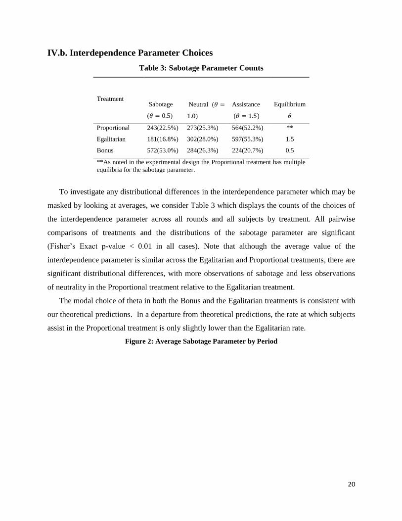
IV.b. Interdependence Parameter Choices

Table 3: Sabotage Parameter Counts

Treatment

Sabotage

(𝜃 = 0.5)

Neutral (𝜃 =

1.0)

Assistance

(𝜃 = 1.5)

Equilibrium

𝜃

Proportional 243(22.5%) 273(25.3%) 564(52.2%) **

Egalitarian 181(16.8%) 302(28.0%) 597(55.3%) 1.5

Bonus 572(53.0%) 284(26.3%) 224(20.7%) 0.5

**As noted in the experimental design the Proportional treatment has multiple

equilibria for the sabotage parameter.

To investigate any distributional differences in the interdependence parameter which may be

masked by looking at averages, we consider Table 3 which displays the counts of the choices of

the interdependence parameter across all rounds and all subjects by treatment. All pairwise

comparisons of treatments and the distributions of the sabotage parameter are significant

(Fisher’s Exact p-value < 0.01 in all cases). Note that although the average value of the

interdependence parameter is similar across the Egalitarian and Proportional treatments, there are

significant distributional differences, with more observations of sabotage and less observations

of neutrality in the Proportional treatment relative to the Egalitarian treatment.

The modal choice of theta in both the Bonus and the Egalitarian treatments is consistent with

our theoretical predictions. In a departure from theoretical predictions, the rate at which subjects

assist in the Proportional treatment is only slightly lower than the Egalitarian rate.

Figure 2: Average Sabotage Parameter by Period

21

In Figure 2, we graph the average 𝜃 in each treatment by period. The horizontal lines in

Figure 2 represent the equilibrium 𝜃 in the Egalitarian and Bonus treatments. In the Proportional

and Egalitarian treatments, the average 𝜃 is larger than 1 which indicates a significant amount of

assistance by the subjects. The Bonus scheme has a lower average 𝜃 across nearly all periods,

with an average 𝜃 of less than one, indicating consistent use of sabotage. The Proportional and

Egalitarian show a clear trend towards assistance as the periods increase (p-values < 0.01 in both

cases). The trend in the Bonus treatment is also significant (p-value < 0.01) but the trend is

towards sabotage.29

To formally test for the differences in the interdependence parameter across treatments, we

use a random effects model with the random effects at the subject level to account for individual

heterogeneity. We use a bootstrap method to calculate standard errors to account for the

asymptotic properties of the estimator on our (relatively) small sample size.30 The results are

reported in Table 4.

29 To test for a period trend we regress theta on the period number, along with a constant. We use a random effect

structure with the random effect on the individual subject to account for individual level heterogeneity and also

bootstrap our standard errors using 1000 replications. 30 As pointed out in Cameron et al (2008), the traditional methods of calculating standard errors in the case of panel

data which may have correlation among clusters (i.e. our sessions) may produce downwardly biased standard error

estimates and hence produce confidence intervals which are too small. To account for this possibility we have also

tested several other models including a random effects model with asymptotic standard errors (iid errors), a model

which accounts for the clustering of errors at the session level, and a model which clusters errors at the subject level.

All results are qualitatively similar and available from the authors upon request.

0

0.2

0.4

0.6

0.8

1

1.2

1.4

1.6

1 2 3 4 5 6 7 8 9 10 11 12 13 14 15 16 17 18 19 20 21 22 23 24 25 26 27 28 29 30

Sab

ota

ge p

aram

eter

Decision Period

Egal Equlibrium - Egal

Prop Bonus

Equlibrium -Bonus

22

Table 4: Treatment Effects

Specification (1) (2) (3) (4)

Dependent variable, 𝜃 Bonus vs.

Prop &Egal

Prop vs.

Egal

Egal vs.

Bonus

Prop vs.

Bonus

Egal 0.04 0.35***

[1 if Egalitarian] (0.05) (0.05)

Bonus -0.33*** -0.31***

[1 if Bonus] (0.05) (0.05)

period 0.00 0.01*** 0.00 0.00

[period trend, t] (0.00) (0.00) (0.00) (0.00)

constant 1.15*** 1.07*** 0.85*** 1.15***

(0.03) (0.04) (0.04) (0.04)

Observations 3240 2160 2160 2160

** significant at 5%; *** significant at 1%. The standard errors are in parentheses and are

calculated from bootstrapping using 1000 replications. All models include a random

effects error structure, with the individual subject as the random effect, to account for the

multiple decisions made by individual subjects.

Given that the Egalitarian and Proportional treatments are similar in the use of sabotage, we

first pool the Egalitarian and Proportional treatments and make a comparison with the Bonus

treatment. The results are reported in column 1 of Table 4. Since the effect of the Bonus

indicator is negative and significant at the 1% level, we conclude that there is significantly more

sabotage in the Bonus treatment relative to the pooled Proportional and Egalitarian treatments. In

column 2, we compare the Egalitarian and the Proportional treatments. The results of the

regression suggest that, at least on average, there is no difference in 𝜃 across the Egalitarian and

Proportional schemes. Hence our data in that regard is mixed. Column 3 compares the

Egalitarian and the Bonus treatments. We see that the Egalitarian indicator is significant and

positive which suggests that the Egalitarian treatment elicits more assistance than the Bonus

treatment. Lastly, we see in column 4 that the Bonus treatment elicits more sabotage relative to

that of the Proportional treatment, which is indicated by the significant and negative coefficient

on the Bonus treatment indicator.

23

V. The Nature of Interdependence

The main purpose of this study is to explore the use of assistance and/or sabotage in the

treatments. In addition to the subject’s choices on the interdependence parameter, we collected

two other pieces of information. These are risk and demographic questionnaires. The risk

questionnaire was implemented as the first part of the Experiment and the demographic data

were collected from the subjects at the conclusion of the Experiment. Table 5 below gives

summary information from these two other sources of information.

Table 5: Summary of Demographic Characteristics and Preferences

Variable Description Mean Std. Dev. Min Max

Quiz number of correct quiz answers 7.33 0.72 6 8

Safe number of safe options 7.88 3.24 0 15

female 1 if female; 0 if male 0.48 0.50 0 1

major 1 if business or econ major 0.64 0.48 0 1

class

number of business or econ

classes taken 5.10 5.85 0 25

Age participant’s age 20.94 3.21 18 41

There is a growing literature with regard to gender differences in choices made in group

settings (see e.g. Cason & Mui 1997; Dufwenberg and Muren 2006, Dato and Nieken 2013). Of

particular interest is the study by Dato and Nieken (2013) that deals directly with sabotage and

gender, although in a tournament setting. The authors use a real effort environment where

subjects are asked to code words into numbers and the agents may sabotage their competitors by

choosing to decrease the number of words that they correctly code. The authors find that

although females and males perform the task at similar levels, males are more likely than females

to use sabotage to enhance their relative standing in the tournament. This previous result

suggests that there is reason to suspect gender differences in the use of sabotage especially in the

Bonus scheme which includes a contest component. To investigate this possibility, Table 6

shows male and female choices in the interdependence parameter across all rounds, by treatment.

We can see from Table 6 that there is considerable variation in the decisions of males and

females in the use of sabotage and assistance.31 The rightmost panel of Table 6 shows the

31Within each treatment there are 36 subjects. In the Egalitarian and Proportional treatments there are 19 females in

each, in the Bonus treatment there are 14 females.

24

choices in the Bonus treatment. The design of this treatment is the most similar to that of Dato

and Nieken (2013). Nonetheless, we find no gender difference in the choices of males and

females. On the other hand, differences across gender are very pronounced with p-values less

than 1% in both the Egalitarian and Proportional payment schemes.

Table 6: Proportion of Interdependence-Choices by Gender

Treatment Proportional Egalitarian Bonus

Assistance

(𝜃 = 1.5)

Sabotage

(𝜃 = 0.5)

Assistance

(𝜃 = 1.5)

Sabotage

(𝜃 = 0.5)

Assistance

(𝜃 = 1.5)

Sabotage

(𝜃 = 0.5)

Male 61.6% 20.2% 71.8% 9.8% 21.2% 54.4%

Female 43.9% 24.6% 40.5% 23.0% 20.0% 50.7%

p-value <0.01 <0.01 0.21

The p-value is from a Fisher’s Exact test of the distribution of 𝜃 and gender. The choices of 𝜃 = 1.0 are

suppressed to highlight differences in assistance and sabotage.

The gender difference is most pronounced in the Egalitarian scheme.32 In this case, male

subjects choose to assist approximately 70 percent of the time, while females choose to assist

only about 40 percent of the time. Even more astounding is the fact that females choose

sabotage in the Egalitarian scheme more than twice as often as males - with more than 1 in 5

choices by females involving the raising of her team member’s cost of effort. It is tempting to

suggest that the gender difference found in the Egalitarian scheme is the result of free-riding or

other regarding behavior but careful comparison with the Proportional scheme shows that this is

likely not the case. Recall that the Proportional payment scheme is designed to give a baseline

measurement on the nature of interdependence among team-members. When comparing this

baseline (i.e. the Proportional treatment) with the nature of interdependence in the Egalitarian

scheme, in which subjects have an (pecuniary) incentive to assist, female choices remain

relatively stable across the two treatments. On the other hand, male choices across the

Proportional and Egalitarian treatments, especially in the use of sabotage, show a propensity for

change. Males become much more likely to assist in the Egalitarian scheme relative to males in

the Proportional scheme. This suggests that the gender difference is driven, not by disparate

32 Wozniak (2014) has subjects choose between a piece rate, a tournament, and an egalitarian payment scheme

(called group pay) and finds that females choose group pay more often than males. Reconciling this preference for

group pay with the relatively stronger preference for sabotage compared to males in the Egalitarian scheme may be

worth exploring in future work.

25

choices of females, but by a reaction to the Egalitarian scheme, rooted in male and not female

behavior.

To more thoroughly consider the impact of gender on the decision to sabotage, we regress the

interdependence parameter – 𝜃 – on a female indicator, a period variable, and indicator variables

for the treatments. The results are included in Table 7 below.

Table 7: Determinants of Sabotage

Treatment(s)

Specification #

Pooled

(1)

Proportional

(2)

Egal

(3)

Bonus

(4)

Egal

Probit

(5)

Dependent variable 𝜃 𝜃 𝜃 𝜃 Sabotage

Female -0.11** -0.11 -0.22*** 0.01 0.15***

[1 if female; 0 if male] (0.04) (0.08) (0.06) (0.07) (0.04)

Egal 0.04

[1 if Egalitarian] (0.05)

Bonus -0.32***

[1 if Bonus] (0.05)

Period 0.00 0.01*** 0.00*** -0.01*** -0.00*

[period trend, t] (0.00) (0.00) (0.00) (0.00) (0.00)

Constant 1.18*** 1.12*** 1.24*** 0.92***

(0.05) (0.06) (0.06) (0.06)

Observations 3240 1080 1080 1080 1080

* significant at 10%; ** significant at 5%; *** significant at 1%. All specifications use

random effects models, with the individual subject as the random effect, to account for the

multiple decisions made by individual subjects. Standard errors are in parenthesis. Columns 1

– 4 bootstrap the standard errors using 1000 repetitions; column 5 uses iid errors with the

errors clustered at the session level. Column 5 shows marginal effects and standard

deviations for the independent variables in a probit regression.

In column 1, we first pool data from all treatments and control for treatment effects by

including an indicator variable for the Bonus and the Egalitarian treatments. Here, the

coefficient of the female indicator is negative and statistically different from zero at the 5% level.

This suggests that, even after controlling for treatment effects, females are less likely to choose a

lower cost for a team-member within the experiment. Column 2 focuses on only the Proportional

treatment. Contrary to the result from Fisher’s exact test, the regression results suggest that males

and females do not differ, as the female indicator is not significant at conventional levels (p-

value >0.10). On the other hand, consistent with the count data, the Egalitarian treatment shows

26

a systematic difference between males and females with females choosing more sabotage than

males. Lastly, we find no gender difference in the Bonus treatment, consistent with the count

data.

In order to quantify the size of the gender disparity in the Egalitarian treatment (Column 5), a

Probit model is employed examining the decision to choose sabotage (i.e. choose 𝜃 = 0.5). We

create an indicator variable, sabotage, which takes the value of 1 when a subject chooses 𝜃 = 0.5

and is zero otherwise. The results indicate that in the Egalitarian treatment females are 15

percentage points more likely to choose sabotage than males. This difference is significant with

a p-value < 0.01.33

Table 8 investigates the robustness of the gender difference in the Egalitarian treatment by

also including control variables for other collected data. After part one of the experiment, but

before subjects participate in the 30 rounds of decision making, the subjects are given a short

quiz over the directions. The quiz is tailored for each different treatment.34In column 1 of Table

8, we include the number of correct responses to the quiz as a control for cognitive ability and

understanding. In column (2), we include the data from part 1 of the experiment. In part 1 of the

experiment, subjects make decisions in a series of lotteries to measure risk preferences. In

column (3) we include the full set of controls.

Considering column (1), we can see that the coefficient on quiz is positive suggesting that as

a subject understands the directions better, the more often she chooses to assist her teammate as

the theory suggests. Even so, the inclusion of quiz only marginally changes the point estimate on

the female indicator and it remains statistically significant at the 1% level. Thus, even after

controlling for cognitive ability and understanding, females still choose to move away from

assistance in the Egalitarian treatment. In column (2) we include information on the risk

questionnaire. When this information is included, the p-value for the female indicator remains

statistically significant at the 1% level suggesting that risk preferences do not explain the gender

difference in the sabotage choice. Lastly, even after including controls for college major, the

33If we perform the same analysis on the Proportional and Bonus schemes we find no gender difference in the Bonus

scheme (p-value = 0.28). The Proportional scheme, on the other hand, has a p-value of 0.10 on the female indicator

which suggests that there is some evidence that females sabotage more than males in the Proportional treatment also. 34The quiz in each treatment is identical except for the last question. The last question is tailored to the specific

treatment. For example, the last question in the Bonus treatment is, “If your result is less than the result of your

group member, will you receive the bonus?”. The result is the sum of the effort choice of each subject with the

random term. The bonus is only awarded to the group member with the largest result.

27

number of economics and business classes taken, and age of the subject, the female indicator

remains statistically significant at the 5% level. Thus we conclude that the gender difference

cannot be attributed to cognitive or risk differences and remains unexplained in our analysis.

Table 8: Determinants of Sabotage in Egalitarian Data

Specification (1) (2) (3)

Dependent variable 𝜃 𝜃 𝜃

Female -0.21*** -0.18*** -0.18**

[1 if female; 0 if male] (0.06) (0.07) (0.08)

Quiz 0.10** 0.10** 0.10*

[number of correct quiz answers] (0.05) (0.04) (0.05)

Safe 0.01 0.01

[number of safe options] (0.01) (0.01)

Major 0.05

[1 if business or econ major] (0.11)

Classes 0.00

[# of econ or business classes] (0.01)

Age 0.01

[participant’s age] (0.02)

Constant 0.46 0.36 0.09

(0.40) (0.39) (0.71)

Observations 1080 1080 1080

* significant at 10%; ** significant at 5%; *** significant at 1%. All

specifications include a period trend (not shown) and use random effects

models, with the individual subject as the random effect, to account for the

multiple decisions made by individual subjects. The standard errors are in

parentheses and are created by bootstrapping.

This gender difference is striking because past experimental research has pointed to a tendency

for females to be more generous than males, for females to be less trusting than males, and for

females to be more reciprocal than males.35 For example, Dufwenberg and Muren (2006) build

on the work by Cason and Mui (1997) in a team dictator game and show that teams consisting of

35 See the excellent review by Croson and Gneezy (2009). The authors show that the evidence of females being

more generous and trusting is mixed. Specifically, the authors argue that these gender differences may be due to

females being more sensitive to the context of the situation of the experiment than males. Nonetheless, it is unclear

to us how this explanation applies to our results and highlights the importance of our result. In particular, it would be

important for the practicing manager to know the contextual situation which makes females more likely to sabotage

a team member in the workplace. Indeed, we see this question as a particularly interesting topic for future research.

28

a female majority are more generous and equalitarian. Our results seem directly at odds with this

since female team members in both the Proportional and Egalitarian treatments exhibit a

relatively stronger preference to sabotage a team member, where in one case they actually have

incentive to assist (i.e., in the Egalitarian scheme) and in the other case (i.e. in the Proportional

scheme) there is no particular incentive to engage in sabotage.

While a more in-depth investigation (a separate research project in itself) of the female

preference for sabotage is called to uncover the precise driving forces behind it, one likely

explanation for our results comes from comparing the baseline (Proportional) treatment with the

Egalitarian treatment. In particular, female choices do not seem to be influenced by the

Egalitarian treatment when compared to the Proportional treatment. This suggests that the

differences are driven mainly by a response to the Egalitarian treatment in males. In a design

which mimics the examination of choices of competition (e.g. Niederle & Vesterlund 2008; Price

2012), Kuhn and Villeval (2013) show that men become much more likely to join teams when

there is an efficiency gain to joining a team. Their experimental design has subjects choosing

either an individual payment or team-based payment scheme. In their baseline they find that

female subjects are more likely than males to select into teams, but this is driven by lower

confidence of females. They find that when there is a large efficiency gain to joining a team,

such as a positive team production externality, males join teams at a higher rate than females.

This suggests that efficiency gains are a rather salient reward for males and not for females. This

is consistent with our results where male and female behavior is only slightly different in the

Proportional treatment and then male choices are driven more towards cooperative behavior in

the Egalitarian treatment when there is an efficiency gain from choosing cooperation in the team

(i.e. choosing to assist).

VI. Concluding Remarks

The use of teams in the production process has become ubiquitous, anchored in the belief

that this mechanism facilitates the exploitation of the complementarities in employees’ skills.

This paper marked the first attempt at empirically examining how some prototypical schemes of

compensating team-members shape this facilitation role, in a setting where one team-member is

explicitly linked to another team member (by having the ability to affect the cost of effort of the

29

team-member). The motivation behind this attempt was the question of whether all such

schemes spur cooperation among team-members? If some schemes produce toxic behaviors,

such as sabotage, then this would be important to identify from a managerial perspective,

especially since there is evidence that such behaviors can be contagious in an organization. In

addressing this question, we first constructed the theoretical device of the Proportional

compensation scheme to (experimentally) uncover the innate nature or tendency of

interdependence among team-members, as the scheme supports assistance, no assistance, or

sabotage among team members as equilibrium outcomes. Unearthing this innate nature is

important as it goes to heart of the issue of whether or not production should be organized in

teams. Then we examined the effects on the nature of interdependence from changing this

scheme to an Egalitarian compensation scheme in one instance, and a Bonus scheme in another

instance.

Experimental evidence (on the Proportional scheme) revealed that there is a natural

predilection for assistance, lending support to the team-basis for organizing production. This

predilection was upended under the Bonus scheme, where sabotage became the preferred mode

of interdependence. This evidence calls into question the wide-spread use of a bonus as a

performance-enhancing device in teams. Under the Egalitarian scheme, assistance was the

preferred mode of interdependence. Importantly, we found no statistically significant (at

conventional levels) difference between the rate of assistance generated in the Egalitarian

scheme and that under the Proportional scheme. Hence, incentivizing assistance doesn’t pay off,

and managers may be well served in reconsidering the use of Egalitarian compensation schemes

in fostering greater team-cooperation. Further, it was found that males and females do not share

the distribution of choices on the mode of interdependence in the Egalitarian and the

Proportional schemes. Robust evidence was uncovered indicating a relatively stronger preference

for sabotage by females compared to males, despite the fact that neither of the two schemes

incentivizes the use of sabotage (and the Egalitarian scheme, in fact, incentivizes, assistance).

This evidence flies in the face of much of the received management-wisdom, where females are

viewed as helping nurture collaboration in teams.

30

References

Analoui, F. (1995). Workplace Sabotage: Its Styles, Motives and Management. The Journal of

Management Development, 14, p.48-66

Bear, J. B., & Woolley, A.W., (2011). The Role of Gender in Team Collaboration and

Performance. Interdisciplinary Science Reviews, 36(2).

Bloomberg L.P. (2010) Women Leaders: The Hard Truth About Soft Skills. Retrieved Jan. 8,

2015 from Bloomberg Business database.

Bose, A., Debashis, P., & Sappington, D. E. (2009). Equal Pay for Unequal Work: Limiting

Sabotage in Teams. Journal of Economics and Management Strategy, 14(1), 25-53

Brown, C.,Monthoux, P., McCullough, A. (1976). The

Access-Casebook. Stockholm, Sweden: TekniskHögskolelitteratur i

Stockholm AB.

Cameron, C., Gelbach, J. B., & Miller, D. L. (2008). Bootstrap-Based Improvements for

Inference with Clustered Errors. The Review of Economics and Statistics, 90(3), 414-427

Charness, G., & Levine, D (2004). Sabotage! Survey Evidence of When it is Acceptable. Center

for Responsible Business, UC Berkeley, Working Paper Series.

Chowdhury, S.M., & Gurtler, Oliver (2013). Sabotage in Contests: A Survey. Working Paper.

Croson, R. and Gneezy, Uri (2009). Gender Differences in Preferences. Journal of Economic

Literature, 47(2), 448-474

Dato, S., Nieken, P. (2014). Gender Differences in Competition and Sabotage, Journal of

Economic Behavior and Organization, v100, 64-80

Dechenaux, E., Kovenock, D., &Sheremeta, R. M. (2014). A survey of experimental research on

contests, all-pay auctions and tournaments. Experimental Economics, Nov 2014

Drago, R. and Garvey, G.T. (1998). Incentives for Helping on the Job: Theory and Evidence.

Journal of Labor Economics, 16, 1-25.

Dufwenberg, M., & Muren, A. (2006).Gender composition in teams. Journal of Economic

Behavior & Organization, 61, 50-54.

Fischbacher, U. (2007), z-Tree: Zurich toolbox Tree: Zurich toolbox for ready-made economic

experiments. Experimental Economics 10(2), pp. 171-178

31

Greiner, Ben. (2004). The Online Recruitment System ORSEE – A Guide for the Organization

of Experiments in Economics. Papers on Strategic Interaction 2003-10, Max Planck Institute of

Economics, Strategic Interaction Group

Hoffman, J.R., and Rogelberg, S.G. (1998). A Guide to Team Incentive Systems. Team

Performance Management, Vol. 4, No. 1, pp. 23-32.

Holt, C. A., &Laury, K. S. (2002). Risk Aversion and Incentive Effects. The American

Economic Review, 92(5), 1644-1655.

Irlenbusch, B., &Ruchala, G. K. (2008). Relative Rewards within Team-Based Compensation.

Labour Economics. 15, 141-167

Krakel, Matthias & Daniel, Muller. (2012). Sabotage in Teams. Economics Letters, 115(2), 289-

292.

Klor, Esteban F.; Kube, Sebastian; Winter, Eyal; Zultan, Ro'i (2011):

Can higher bonuses lead to less effort? Incentive reversal in teams, Discussion paper

series // Forschungsinstitut zur Zukunft der Arbeit, No. 5501.

Lazear, E. P., &Oyer, P. (2009). Personnel Economics. Handbook of Organizational Economics.

List, J. A. (2007).On the Interpretation of Giving in Dictator Games. .Journal of Political

Economy, 482-493.

Mas, A. &Moretti, E. (2009). Peers at Work. American Economic Review.

September, 99(1): 112-145.

McAfee, R. P., & McMillan, J. (1991). Optimal Contracts for Teams. International Economic

Review, 32(3), 561-577.

Nawrocki, J., & Wojciechowski, A. (2001). Experimental Evaluation of Pair Programming.

Proc.12th European Software Control and Metrics Conf., pp. 269-276

Price, Curtis R. (2012). Gender Competition and Managerial Decisions. Management Science,

58(1), 114-122

Price, Curtis R. & Sheremeta, Roman (forthcoming). Endowment Origin, demographic effects

and individual preferences in contests. Journal of Economics and Management Strategy

Veblen (1917). An Inquiry into the Nature of Peace, and the Terms of Its Perpetuation, p. 168.

Winter, E. (2009). Incentive reversal. American Economic Journal: Microeconomics

1(2): 133–147

32

33

Appendix: Experimental Instructions

GENERAL INSTRUCTIONS

This is an experiment in the economics of decision making. Various research agencies have

provided funds for this research. The instructions are simple. If you follow them closely and make

appropriate decisions, you can earn an appreciable amount of money.

The experiment will proceed in two parts. The currency used in Part 1 of the experiment is U.S.

Dollars. In part 2 of the experiment you will earn points. At the end of the experiment, points will be

converted to U.S. Dollars at a rate of _300_ points to _1_ dollar. Your earnings today will be calculated as

the sum of your earnings in each part of the experiment plus a $10 show up payment. At the end of

today’s experiment, you will be paid in private and in cash. 12 participants are in today’s experiment.

It is very important that you remain silent and do not look at other people’s work. If you have any

questions, or need assistance of any kind, please raise your hand and an experimenter will come to you. If

you talk, laugh, exclaim out loud, etc., you will be asked to leave and you will not be paid. We expect and

appreciate your cooperation.

At this time we will proceed to Part 1.

INSTRUCTIONS FOR PART 1

YOUR DECISION

In this part you will be asked to make a series of choices in decision problems. How much you

receive will depend partly on chance and partly on the choices you make. The decision problemsare not

designed to test you. What we want to know is what choices you would make in them. The only right

answer is what you really would choose.

For each line in the table in the next page, please state whether you prefer option A or option

B.Notice that there are a total of 15 lines in the table but just one line will be randomly selected for

payment. You do not know which line will be paid when you make your choices. Hence you should pay

attention to the choice you make in every line. After you have completed all your choices, a token will be

randomly drawn out of a bingo cage containing tokens numbered from 1 to 15. The token number

determines which line is going to be paid.

Your earnings for the selected line depend on which option you chose:If you chose option A in

that line, you will receive $1. If you chose option B in that line, you will receive either $3 or $0. To

determine your earnings in the case you chose option B there will be a second random draw. A token will

be randomly drawn out of the bingo cage now containing twenty tokens numbered from 1 to 20. The

token number is then compared with the numbers in the line selected (see the table). If the token number

34

shows up in the left column you earn $3. If the token number shows up in the right column you earn $0.

Are there any questions?

35

Participant ID _________

Decis

ion

no.

Option

A

Option

B

Please

choose

A or B

1 $1 $3 never

$0 if 1,2,3,4,5,6,7,8,9,10,11,12,13,14,15,

16,17,18,19,20

2 $1 $3 if 1 comes out of the bingo cage

$0 if 2,3,4,5,6,7,8,9,10,11,12,13,14,15,

16,17,18,19,20

3 $1 $3 if 1 or 2

$0 if 3,4,5,6,7,8,9,10,11,12,13,14,15,

16,17,18,19,20

4 $1 $3 if 1,2 or 3

$0 if 4,5,6,7,8,9,10,11,12,13,14,15,

16,17,18,19,20

5 $1 $3 if 1,2,3,4

$0 if 5,6,7,8,9,10,11,12,13,14,15,

16,17,18,19,20

6 $1 $3 if 1,2,3,4,5

$0 if 6,7,8,9,10,11,12,13,14,15,

16,17,18,19,20

7 $1 $3 if 1,2,3,4,5,6 $0 if 7,8,9,10,11,12,13,14,15,16,17,18,19,20

8 $1 $3 if 1,2,3,4,5,6,7 $0 if 8,9,10,11,12,13,14,15,16,17,18,19,20

9 $1 $3 if 1,2,3,4,5,6,7,8 $0 if 9,10,11,12,13,14,15,16,17,18,19,20

10 $1 $3 if 1,2,3,4,5,6,7,8,9 $0 if 10,11,12,13,14,15,16,17,18,19,20

11 $1 $3 if 1,2, 3,4,5,6,7,8,9,10 $0 if 11,12,13,14,15,16,17,18,19,20

12 $1 $3 if 1,2, 3,4,5,6,7,8,9,10,11 $0 if 12,13,14,15,16,17,18,19,20

13 $1 $3 if 1,2, 3,4,5,6,7,8,9,10,11,12 $0 if 13,14,15,16,17,18,19,20

14 $1 $3 if 1,2, 3,4,5,6,7,8,9,10,11,12,13 $0 if 14,15,16,17,18,19,20

36

15 $1 $3 if 1,2, 3,4,5,6,7,8,9,10,11,12,13,14 $0 if 15,16,17,18,19,20

37

INSTRUCTIONS FOR PART 2 – Egalitarian Example

YOUR DECISION

Part 2 consists of 30 decision making rounds. In each round one other participant is randomly

assigned to you to form a two person group. During each round, you only interact with the participant in

your group.At the beginning of each new round you are randomly and anonymously rematched with a

different participant to form a new two person group. The identities of your group members are never

revealed to you.

The costs and payoffs are given in points. At the end of the experiment the amount of points you

accumulate will be converted to U.S. Dollars at a rate of _300_ points to _1_ dollar.

In each round you will make two decisions.

Decision 1: Types

You choose a type for your group member and your group member will choose your type. There are three

possible types to choose from – type A, type B, or type C. Each type has a different cost structure of the

decisions to be made later. Type A has the highest cost structure, type B has the second highest cost

structure and type C has the lowest cost structure.

Keep in mind that you do not choose your own type. You choose the type for your group member and

your group member will choose your type.

Once your group member has chosen your type, you will then be told which type you are for that round.

You should record your type on the record sheet which was given to you.

Decision 2: Choose a number from 0 to 65

Your second decision will be to choose a number from 0 to 65. Each number you choose will have an

associated cost which is determined by your type (see the appropriate cost sheet). You should record your

choice of number on the record sheet which was given to you.

Once you have made both decisions, the computer will make a series of calculations and the number of

points that you earn in that round will be displayed on the computer screen. These are outlined in detail

in the next section. After making these two decisions in a round, the round is concluded and you will be

rematched with another subject to form a new two person group. This will be repeated 30 times for a total

of 30 decision making rounds. At the conclusion of this part, two of the 30 rounds will be randomly

selected and you will be paid for your performance in those two rounds.

Procedure of a round:

1. You choose a type for your group member and your group member will choose your type. There

are three possible types to choose from – type A, type B, or type C. Each type has a different cost

structure of the decisions to be made later. Type A has the highest cost structure, type B has a

lower cost structure and type C has the lowest cost structure.

2. Once your group member has chosen your type, you will be instructed which cost record sheet to

consider for your next decision.

38

3. You choose a number from 0 to 65. Your choice does not have to be a whole number (i.e.

decimals are allowed).

4. For each group member a random number is drawn between -10 and 10. Every number in that

range is equally likely to be picked. (Your random number and the random number of your group

member are not revealed to you.) The computer calculates the payoffs on the basis of your chosen

numbers and the random numbers. This happens as follows:

First the Result is calculated. The Result of each participant is the sum of his chosen number and his/her

individual random number. Result = chosen number + individual random number

Your round payoff is equal to 25 times the sum of your Result and your group member’s Result minus the

cost of your chosen number. Your Round Payoff = 25 x (your Result + group member’s Result) – (cost of your chosen number)

Remember, the cost of your chosen number issubtracted from your payoff as shown above. This may

result in losses or negative points. The cost of your chosen number depends on your type which was

chosen for you by your group member and are shown in the cost table. If a round is selected for

payment in which you have earned negative points, you will pay the losses out of your show up payment

and/or earnings from Part 1 of the experiment.

5. You are rematched with another subject in the experiment and the next round starts.

At the end of the experiment, we will randomly draw two numbers from the bingo cage containing

numbers 1-30. These two numbers represent the two rounds of part 2 which will be paid. Since you do

not know which two rounds are paid, you should pay particular attention to all your decisions so as to

maximize your earnings from this part of the experiment. Any losses will be paid out of your show up

payment and/or earnings from Part 1 of the experiment.

Your total payment from the experiment is the sum of your $10 participation payment, plus your earnings

in the two randomly selected rounds of part 2, along with your earnings from your decisions in part 1.

Are there any questions?

39

Personal Record Sheet for Part 2

Participant ID _________

Round Your Type Your Chosen

Number Earnings

1

2

3

4

5

6

7

8

9

10

11

12

13

14

15

16

17

18

19

20

21

22

23

24

25

26

27

28

29

30

40

Appendix – Cost sheet example – Type A

Type A Chosen Number Cost

Chosen Number Cost

Chosen Number Cost

0 0.0

26 676.0

52 2704.0

1 1.0

27 729.0

53 2809.0

2 4.0

28 784.0

54 2916.0

3 9.0

29 841.0

55 3025.0

4 16.0

30 900.0

56 3136.0

5 25.0

31 961.0

57 3249.0

6 36.0

32 1024.0

58 3364.0

7 49.0

33 1089.0

59 3481.0

8 64.0

34 1156.0

60 3600.0

9 81.0

35 1225.0

61 3721.0

10 100.0

36 1296.0

62 3844.0

11 121.0

37 1369.0

63 3969.0

12 144.0

38 1444.0

64 4096.0

13 169.0

39 1521.0

65 4225.0

14 196.0

40 1600.0

15 225.0

41 1681.0

16 256.0

42 1764.0

17 289.0

43 1849.0

18 324.0

44 1936.0

19 361.0

45 2025.0

20 400.0

46 2116.0

21 441.0

47 2209.0

22 484.0

48 2304.0

23 529.0

49 2401.0

24 576.0

50 2500.0

25 625.0

51 2601.0