Embed Size (px)
Citation preview
DI
SC
US
SI
ON
P
AP
ER
S
ER
IE
S
Forschungsinstitut zur Zukunft der ArbeitInstitute for the Study of Labor
Will GDP Growth Increase Happiness inDeveloping Countries?
IZA DP No. 5595
March 2011
Andrew E. ClarkClaudia Senik
Will GDP Growth Increase Happiness in
Developing Countries?
Andrew E. Clark Paris School of Economics
and IZA
Claudia Senik Paris School of Economics
and IZA
Discussion Paper No. 5595 March 2011
IZA
P.O. Box 7240 53072 Bonn
Germany
Phone: +49-228-3894-0 Fax: +49-228-3894-180
E-mail: [email protected]
Any opinions expressed here are those of the author(s) and not those of IZA. Research published in this series may include views on policy, but the institute itself takes no institutional policy positions. The Institute for the Study of Labor (IZA) in Bonn is a local and virtual international research center and a place of communication between science, politics and business. IZA is an independent nonprofit organization supported by Deutsche Post Foundation. The center is associated with the University of Bonn and offers a stimulating research environment through its international network, workshops and conferences, data service, project support, research visits and doctoral program. IZA engages in (i) original and internationally competitive research in all fields of labor economics, (ii) development of policy concepts, and (iii) dissemination of research results and concepts to the interested public. IZA Discussion Papers often represent preliminary work and are circulated to encourage discussion. Citation of such a paper should account for its provisional character. A revised version may be available directly from the author.

IZA Discussion Paper No. 5595 March 2011
ABSTRACT
Will GDP Growth Increase Happiness in Developing Countries?* This paper asks what low-income countries can expect from growth in terms of happiness. It interprets the set of available international evidence pertaining to the relationship between income growth and subjective well-being. Consistent with the Easterlin paradox, higher income is always associated with higher happiness scores, except in one case: whether growth in national income yields higher well-being is still hotly debated. The key question is whether the correlation coefficient is “too small to matter”. The explanations for the small correlation between national income growth and subjective well-being over time appeal to the nature of growth itself (from negative side-effects, such as pollution), and to the psychological importance of relative concerns and adaptation. The available evidence contains two important lessons: income comparisons do seem to affect subjective well-being, even in very poor countries; however, adaptation may be more of a rich-country phenomenon. Our stand is that the idea that growth will increase happiness in low-income countries cannot be rejected on the basis of the available evidence. First, cross-country time-series analyses are based on aggregate measures, which are less reliable than those at the individual level. Second, development is a qualitative process involving take-off points and thresholds. Such regime changes are visible to the eye through the lens of subjective satisfaction measures. The case of Transition countries is particularly impressive in this respect: average life satisfaction scores closely mirrored changes in GDP for about the first ten years of the transition process, until the regime became more stable. The greater availability of subjective measures of well-being in low-income countries would greatly help in the measurement and monitoring of the different stages and dimensions of the development process. JEL Classification: D63, I3, O1 Keywords: income, subjective well-being, comparisons, adaptation, development Corresponding author: Andrew Clark PSE 48 Boulevard Jourdan 75014 Paris France E-mail: [email protected]
* We thank Hélène Blake for precious research assistance and CEPREMAP for financial support. We are very grateful to Emmanuel Commolet, Nicolas Gury and Oliver Charnoz for incisive comments on a previous draft, and Alpaslan Akay, Alexandru Cojocaru, Luca Corazzini, Ada Ferrer-i-Carbonell, Armin Falk, Carol Graham, Olof Johansson-Stenman, John Knight, Andrew Oswald, Bernard Van Praag, Mariano Rojas, Russell Smyth, and Oded Stark for advice.

I. INTRODUCTION ..................................................................................................... 3 I.1 The data used in the paper.............................................................................................................................. 4 I.2 Subjective well-being measures: why use them and are they reliable?....................................................... 5 I. THE PARADOXICAL RELATIONSHIP BETWEEN GROWTH AND WELL-BEING................................................................................................................................. 10
I.1. Income raises happiness in the cross section .............................................................................................. 10 a. Within-country cross-section.................................................................................................................. 10 b. Cross-sections of countries ..................................................................................................................... 11 c. A positive relation in individual panel data ............................................................................................ 13
I.2. The diminishing returns to income growth ................................................................................................ 13 a. Is there a threshold in the utility of growth? ........................................................................................... 14 b. But the happiness-log GDP per capita gradient does not tend to zero. ................................................... 15
1.3 “Rather than diminishing marginal utility of income, there is a zero marginal utility of income” ....... 16 I.4 Is the time-series correlation small enough to ignore? ...................................................................... 18
A note on statistical power ............................................................................................................................... 19 I.5 Subjective well-being and the business cycle............................................................................................... 20 II. EXPLANATIONS RELATED TO GROWTH ITSELF: CHANNELS AND NEGATIVE SIDE-EFFECTS .................................................................................... 22 II.1 Quality of Life: channels from GDP growth to happiness ....................................................................... 22
a. Cross-section correlation between GDP growth and Quality of Life indicators........................................... 23 b. Time-series correlation between GDP growth and Quality of Life indicators ............................................. 24
II. 2. Negative side-effects of growth ................................................................................................................. 25 III. EXPLANATIONS RELATED TO THE HAPPINESS FUNCTION ITSELF (HUMAN BEINGS ARE SOCIAL ANIMALS)........................................................... 26 III.1. Income comparisons................................................................................................................................. 26
a. Evidence in Developed Countries ................................................................................................................ 28 b. Evidence in LDCs ........................................................................................................................................ 30 c. Absolute versus relative poverty .................................................................................................................. 34
III.2. Adaptation.................................................................................................................................................. 36 a. Evidence in Developed Countries ................................................................................................................ 37 b. Evidence in LDCs................................................................................................................................... 38
III.3 Bounded scales: What exactly is relative?................................................................................................ 40 IV. CONCLUSIONS AND TAKE-HOME MESSAGES: HOW CAN WE USE SUBJECTIVE VARIABLES IN ORDER TO UNDERSTAND THE GDP-HAPPINESS RELATIONSHIP?..................................................................................................... 41
REFERENCES ......................................................................................................... 45
2
I. INTRODUCTION
Is income growth the only thing that matters in development, and does it raise the level of
well-being of the population? De facto, economic development is generally identified with
growth in GDP per capita: International organizations, such as the United Nations
Organization, the OECD, the World Bank and the International Monetary Fund, classify
countries as developed, intermediate or low-development, depending on whether they are
above or below certain thresholds of GDP per capita. However, development is of course
more than just income growth. It is a multi-dimensional process, which involves not only a
quantitative increase in capital accumulation, production and consumption, but also
qualitative social and political changes that enlarge the choice set of the individuals
concerned. Institutional progress, human rights, democracy, gender equality and other
capacities are an integral part of development. We can then ask whether these qualitative
objectives can be attained by maximizing GDP. And in addition, we might worry that income
growth will yield negative side-effects, which reduce well-being, such as environmental
externalities, the destruction of traditional social links, the concentration of the population in
urban and suburban centres, the development of work-related stress, and so on.
“Is growth obsolete?” The provocative title of the paper by William Nordhaus and James
Tobin (1973) reflects the radical questioning of growth as an engine of well-being. Although
the authors answer this question in the negative, many economists and social scientists have
come to the conclusion that, in developed countries, economic growth per se has little impact
on well-being and should therefore not be the primary goal of economic policy (see Oswald,
1997). How much of this argument can we extend to developing countries? Or should we
follow the proposition of Inglehart et al. (2008) that material growth, as measured by GDP per
capita, is welfare-improving in developing countries, as it takes people out of poverty and
precarity, but that it is useless in modern and “post-modern” societies where survival is taken
for granted and human development becomes the only valuable goal?
This paper will address the relationship between GDP growth and well-being in developing
countries through the lens of subjective well-being measures, i.e. self-declared satisfaction
3
judgements collected in surveys of nationally-representative samples of the population over
the world. Using these measures as a shortcut to people’s well-being, we will try to see
whether GDP growth is really a proxy for and a valuable route to happiness.
One of the most important but equally most controversial issues in the subjective well-being
literature is precisely the income-happiness relationship. In a famous article, Easterlin (1974)
ironically asked whether “raising the incomes of all will raise the happiness of all?” This was
based on the observation that average happiness measures remained flat over the long-run in
countries which had experienced high rates of GDP growth. The income-happiness nexus has
been vividly debated for the past two decades by economists, psychologists and political
scientists. However, most of the evidence to date on the relationship between income and
subjective well-being is based on developed countries. Is the Easterlin paradox also valid for
developing countries, or is it a rich country phenomenon?
This paper presents an overview of the evidence that has accumulated during the past twenty
years of research and illustrates some of the findings using a widely used international
database (the World Values Survey, 1981-2005) containing individual life satisfaction and
happiness information. In a first section, we present the relationship between income, income
growth and subjective well-being and ask to what extent the patterns usually observed in
developed countries also hold in developing countries. We discuss the potential existence of a
threshold effect in the welfare returns of growth, where the latter are higher in low- as
opposed to high-income countries. Sections 2 and 3 then present the classic explanations of
the Easterlin paradox and their relevance to developing countries. Here, we distinguish the
positive and negative side-effects of growth, and the limits to the way in which income can
produce subjective well-being that stem from human nature itself (comparison and adaptation
effects). Finally, we provide some reasons why we believe that cross-section and panel
analysis based on individual data is more reliable than that using aggregated times-series.
Accordingly, we conclude that the positive income-well-being gradient, supported by
individual and cross-sectional data, is difficult to dismiss.
I.1 The data used in the paper
This paper essentially hinges on results in the existing literature. However, we have added a
number of figures of our own, using the five waves of the well-known World Values Survey
(WVS, 1981-2008) database covering 105 countries, including high-income, low-income and
4

Transition countries, which account for 90% of the world’s population. Happiness measures
were mostly taken from the WVS and the European Social Survey (ESS): this is the case for
250 out of 368 observations. When happiness data was missing, we used information from the
ISSP (101 observations) and 17 observations from the 2002 Latinobarometer. All of these
datasets are available at http://worldvaluessurvey.org. The happiness and life satisfaction
questions were administered in the same format in all these surveys, with equivalent
translations for all countries. The wording of the Happiness question was: “If you were to
consider your life in general these days, how happy or unhappy would you say you are, on the
whole?: 1. Not at all happy; 2. Not very happy; 3. Fairly happy; 4. Very happy”. In the WVS,
the wording of the Life Satisfaction question was: “All things considered, how satisfied are
you with your life as a whole these days?: 1(dissatisfied) … 10 (very satisfied)”. The surveys
cover representative samples of the population of participating countries, with an average
sample size of 1400 respondents at each wave. We calculated the national average value of
the answers to each of these questions (treating them as continuous variables). We also
created a misery index defined as the percentage of people who declare themselves to be very
happy, or very satisfied, minus the percentage of respondents declaring themselves to be not
at all happy, or not at all satisfied. As the results from the two aggregate well-being measures
were very similar, we only present here the Figures based on average well-being.
The paper also appeals to a measure of trust, which is available in the WVS: “Generally
speaking, would you say that most people can be trusted or that you can’t be too careful in
dealing with people?: 1. Most people can be trusted; 0 . Can't be too careful”. The GDP per
capita and annual GDP growth information comes from Heston, Summers and Aten – the
Penn World Table. We also use other quantitative indicators which are available in the World
databank, such as the Gini measure of income inequality, women’s fertility rates, adult
literacy rates, and life expectancy at birth (see http://data.worldbank.org/). The qualitative
indicators of governance were taken from Freedom House and Polity IV
(http://www.qog.pol.gu.se/, http://www.freedomhouse.org, http://www.govindicators.org, and
http://www.systemicpeace.org/polity/polity4.htm ). All these data are available from the
World Data Bank: http://www.worldvaluessurvey.org.
I.2 Subjective well-being measures: why use them and are they reliable?
The critical quality of subjective well-being is that it is self-reported. Instead of a third person
designing some set of criteria (income, health, education, housing etc.) which will define
5
how well an individual is doing, individuals themselves are asked to provide a summary
judgement of the quality of their life. While some have doubted the usefulness of subjective
measures, we think that there are fairly compelling reasons to include them in the Economists’
arsenal.
Think of an individual’s level of well-being as being some appropriately-weighted sum of all
of the aspects of life that matter to her. There are at least two significant obstacles for it to be
measured objectively. The first is that we need to be sure that we cover all of the aspects of
life that are important to the individual, and it seems a priori difficult to make up a definitive
measurable list of these. The second problem is that we have to apply appropriate weights to
construct the final well-being index. This might appear problematic right from the start: in the
context of the aggregate data used in the Human Development Index, for example, how much
is literacy worth in terms of life expectancy? Moreover, it would appear extremely likely that
any such weighting will differ between individuals, and probably in ways that it is not easy to
observe. It is consequently very tempting to sidestep the difficulties involved by asking
individuals to make these calculations themselves, in responding to evaluative questions about
their own lives.
The well-being questions asked in this context are often very simple ones, such as “How
dissatisfied or satisfied are you with your life overall?” (from the British Household Panel
Survey), which is answered on a seven-point scale, with one referring to “Not satisfied at all”,
four to “Neither satisfied nor dissatisfied” and seven to “Completely satisfied”. Alternatively
individuals may be asked about their happiness, as in the following question from the
American General Social Survey (GSS): “Taken all together, how would you say things are
these days, would you say that you are very happy, pretty happy, or not too happy?” Other
questions may refer to positive and negative affect or mental health.
These questions are increasingly widely included in surveys across the social sciences. One
reason for their popularity is that they are simple to put into questionnaires, as probably the
majority of those that appear are single-item (although there are very many multiple-item
scales that are also available in the literature: see
http://acqol.deakin.edu.au/instruments/instrument.php for a summary of some of these). A
second point is that the vast majority of respondents seem to understand the question: non-
response rates are very low. The third reason, which from our point of view is the most
6

important, is that the answers to these questions do seem to pick up how well people are
doing.
This last statement might seem to be rather uncontroversial: after all, we would expect a
question on life satisfaction to measure exactly that. The potential problem lies exactly in the
subjectivity of the reply. In particular, if individuals understand the question differently, or
use the response scales differently, then there is a danger that someone who answers six on a
one to seven satisfaction scale is no better off than another person who has given an answer of
five. Luckily there is by now a varied body of evidence suggesting that these subjective well-
being measures do contain valid information.
A first point to make is that subjective well-being measures are well-behaved, in the sense
that many of the correlations make sense. In cross-section data, variables reflecting marriage,
divorce, unemployment, birth of first child and so on are typically correlated with individuals’
subjective well-being in the expected direction.1 If the answers to well-being questions were
truly random, then no such relationship would be found.
We want to know whether asking A how happy she is will provide information about her
unobserved real level of happiness. One simple check, called Cross-Rater Validity, is to ask B
whether she thinks A is happy. This work has been carried out in a number of settings (see
Sandvik et al., 1993, and Diener and Lucas, 1999), including asking friends and family, or the
person who administered the interview. Alternatively, we can use individuals who do not
know the subject: B may be shown a video recording of A, or may read a transcription of an
open-ended interview with A. In all cases, B’s evaluation of the respondent’s well-being
matches well with the respondent’s own reply.
Another approach to validation consists in relating well-being scores to various physiological
and neurological measures. It has been shown that answers to well-being questions are
correlated with facial expressions, such as smiling and frowning, as well as heart rate and
blood pressure. The medical literature has shown that well being scores are correlated with
digestive disorders and headaches, coronary heart disease and strokes. Research has also
looked at physical measures of brain activity. Particular interest has been shown in the
1 See, for example, the findings in Di Tella, MacCulloch and Oswald (2003), based on the analysis of the well-being reported by levels of a quarter of a million randomly-sampled Europeans and Americans from the 1970s to the 1990s. 7

differences in brain wave activity between the left and right prefrontal cortexes, where the
former is associated with positive and the latter with negative feelings. These differences can
be measured using electrodes on the scalp or scanners. Research has shown (for example,
Urry et al., 2004) that these differences in brain activity are correlated with individual well-
being responses. These measures of brain asymmetry have been shown to be associated with
cortisol and corticotropin releasing hormone (CRH), which regulate the response to stress, and
antibody production in response to influenza vaccine (Davidson, 2004). Consistent with
subjective well-being and brain asymmetry measuring the same underlying construct, individuals
reporting higher life satisfaction scores were less likely to catch a cold when exposed to a cold
virus, and recovered faster if they did (Cohen et al., 2003).
The last block of evidence that people “mean what they say” is that, in data following the same
individual over a long period of time, those who say that they are dissatisfied with a certain
situation are more likely to take observable action to leave it. This phenomenon is apparent in the
labor market, where the job satisfaction that the individual reports at a certain point in time is a
good predictor of her being observed in the future to have quit her job (examples are Freeman,
1978, Clark et al., 1998, Clark, 2001, and Kristensen and Westergaard-Nielsen, 2006). One
important subsidiary finding in this literature is the job satisfaction predicts quits even when we
take into account the individual’s wages and hours of work. This prediction of future behavior
seems to work for the unemployed as well as for the employed. Clark (2003) shows that mental
stress scores on entering unemployment in BHPS data predict the length of the unemployment
spell, with those who suffered the sharpest drop in well-being upon entering unemployment
having the shortest spell. This finding has been replicated in using the life satisfaction scores in
GSOEP data by Clark et al., 2010). Outside of the labor market, well-being scores have been
shown to predict the length of life (Palmore, 1969, Danner et al., 2001). Satisfaction measures
have also recently been shown to predict future marital break-up (Gardner and Oswald, 2006,
Guven et al., 2010).
One potential use of the analysis of subjective well-being is that it arguably provides us with
information on trade-offs between different aspects of an individual’s life. If one extra hour of
work per week has the same effect on well-being as does 80 Euros in additional earnings per
month, then the shadow wage (the wage that would compensate for one extra hour of work) is
around 18 Euros and 50 cents per hour. Some of examples of these well-being trade-offs have
appeared in the recent literature. For example, Blanchflower and Oswald (2004, p 1381),
using American and British data, came to the conclusion that: “To compensate men for
8

unemployment, it would take a rise in income at the mean of approximately $60000 per
annum. A lasting marriage is worth 100000$ per annum (when compared to widowhood or
separated)”.
This capacity of subjective data to weight the different dimensions of development one
against the other (to calculate marginal rates of substitution between two dimensions) is
particularly adapted to the multidimensionality of economic development. The structure of the
well-being equation, as estimated in a country, can be seen as a synthetic measure that would
have aggregated the different arguments of a social welfare function. The usual problem of
the social planner (and of the social choice school of normative economics) is indeed to
decide on the weights that should be attached to the different arguments of the social objective
function. Subjective measures allow avoiding this obstacle by measuring directly the synthetic
result of the weighting alchemy made by individuals themselves. An illustration of this is the
paper by Di Tella and MacCulloch (2008, pp.31-33), where the authors use the American
GSS and the Eurobarometer to estimate national welfare functions. They propose such
marginal rates of substitution:
- Life expectancy / income: “A person who expects to live one year longer due to the
reduction in the risk of death is willing to pay $5052 in annual income in exchange
(6.6% of GDP per capita)”.
- Life expectancy / unemployment: “In terms of the unemployment rate, denying an
individual one year of life expectancy has an equivalent cost to increasing the
unemployment rate by 1.1 percentage point”.
- Pollution/GDP: “a one standard deviation increase in SOx emissions, equal to a rise
in 23kg per capita, has a decrease on well-being equivalent to a 15% drop in the level
of GDP per capita.”
- Inflation/unemployment: “a 1% point rise in the level of inflation reduces happiness
by as much as a 0.3 percentage point increase in the unemployment rate”.
- Crime/GDP: “a rise in violent crime from 242 to 388 assaults per 100000 people in
the United States (i.e. a 60% rise) … would be equivalent to a drop of approximately
3.5% in GDP per capita”.
9

- Working hours/GDP: “a 1% rise in working hours would have to be compensated by a
2.4% rise in GDP per capita (to leave happiness unchanged)”.
These examples illustrate the capacity of subjective well-being measures to serve as a useful
tool for public policy aimed at maximizing well-being as countries develop.
Before we turn to the evidence on growth and subjective well-being, we should warn the
reader of two abusive approximations contained this paper. First, we use the terms happiness,
life satisfaction and well-being indiscriminately. Second, we treat these measures as though
they were cardinal, although they are more properly ordinal. In doing so, as do the bulk of
economists working on happiness measures, we follow the route opened by Ferrer-i-
Carbonnell and Frijters (2004).
I. THE PARADOXICAL RELATIONSHIP BETWEEN GROWTH AND WELL-
BEING
One of the main catalysts in the voluminous and rapidly expanding literature on income and
happiness has been Easterlin’s seminal article (1974; updated in 1995), setting out the
‘paradox’ of substantial real income growth in Western countries over the last fifty years, but
without any corresponding rise in reported happiness levels. This finding is paradoxical for a
number of reasons. First it runs counter to the popular prior that increased material wealth and
greater freedom of choice should go hand-in-hand with higher well-being. In a way, our
societies are organized on this implicit principle. Second, it seems to contradict a large body
of scientific empirical evidence based on cross-sections of countries, and on within-country
individual panel data. This section presents and discusses the available evidence on these
contradictory findings, and asks whether the Easterlin paradox is a rich-country phenomenon
or also something relevant for policy-makers in developing countries. A summary of the
wide-ranging data sources and results appears in Appendix A.
I.1. Income raises happiness in the cross section
a. Within-country cross-section
“As far as I am aware, in every representative national survey ever done, a significant
bivariate relationship between happiness and income has been found” (Easterlin 2005, p. 67).
10

Almost all of the empirical work based on within-country surveys include individual income
or household income (or more precisely, the log of income) as a control variable to explain
well-being. Log income invariably attracts a positive and statistically significant coefficient,
of considerable size. It is typically one of the most important correlates of self-declared
happiness. “When we plot average happiness versus average income for clusters of people in
a given country at a given time…rich people are in fact a lot happier than poor people. It’s
actually an astonishingly large difference. There’s no one single change you can imagine that
would make your life improve on the happiness scale as much as to move from the bottom 5
percent on the income scale to the top 5 percent” (Frank, 2005, p. 67). This holds for both
developed and developing countries, even if it has sometimes been suggested that the income-
happiness slope is larger in developing or transition than in developed economies (see Clark
et al., 2008, for a survey).
Layard et al. (2010) for instance, report that within a country, a unit rise in log income raises
individual self-declared happiness by 0.6 units on average (on a 10-point scale). Stevenson
and Wolfers (2008, p. 13) estimate the within-country well-being-income gradient over each
of the countries available in a number of international datasets (the American General Social
Survey, the World Values Survey, the Gallup World Poll, etc.). They conclude that: “Overall,
the average well-being-income gradient is 0.38, with the majority of the estimates between .25
and .45 and 90 percent are between 0.07 and 0.72. In turn, much of the heterogeneity likely
reflects simple sampling variation: the average country-specific standard error is 0.07, and
90 percent of the country-specific regressions have standard errors between 0.04 and 0.11”.
As an illustration, Figure 1.A depicts the household income-happiness gradient in the United
States. The fitted relationship is well-described by a log-linear function. The same findings
hold in a series of surveys covering developing countries. Figure 1.B shows the income
decile-happiness gradient in China in 2007 (based on World Values Survey data): the same
positive relationship appears. In general, the fact that in a given society the rich are happier
than the poor is a well-established and undisputed empirical finding in this literature.
b. Cross-sections of countries
The empirical evidence is even more conclusive and consensual regarding the income-
happiness gradient across countries. Deaton (2008), for example, finds an elasticity of 0.84
between log average income and average national satisfaction across a large set of nationally
11

representative samples of individuals living in 129 developed and developing countries,
collected by the 2006 Gallup World Poll. In the same spirit, Inglehart (1990, chapter 1)
analyzes data from 24 countries at different levels of development and finds a 0.67 correlation
between GNP per capita and life satisfaction. In a more recent paper, Inglehart et al. (2008)
report a correlation of 0.62 using all available waves of the World Values Survey. Wolfers
and Stevenson (2008, p. 12), using a very comprehensive set of data, uncover “a between-
country well-being-GDP gradient [..] typically centered around 0.4”.2 In the surveys
analyzed by Inglehart et al. (2008), 52% of the Danes indicated that they were very satisfied
with their life (with a score of over 8 on a 10-point scale) and 45% said they were very happy.
On the contrary, in Armenia only 5% said they were very satisfied and 6% very happy.
Figure 2.A (taken from Inglehart et al., 2008) shows the concave relationship between income
per capita and average happiness across developed, developing and Transition countries of the
world, over the 1995-2007 period. A similar graph appears in Deaton (2008) based on the
World Values Survey (1996) and the Gallup World Poll (2006), which we reproduce here as
Figure 2.B. As shown in Figure 2.C, “Each Doubling of GDP is Associated with a Constant
Increase in Life Satisfaction” across countries (Deaton, 2008). Figure 2.D illustrates the good
fit of a log-linear relationship between income per capita and average life satisfaction across
countries of the world, in the late 2000s, using the most recent waves of the World Values
Survey.
Many other contributions to the “macroeconomics of happiness” have documented the fact
that individuals in general report higher happiness and life satisfaction scores in higher-
income countries (see for example Blanchflower, 2008), even if certain types of societies
seem to be more conducive to happiness than others (Inglehart et al., 2008). In Figure 2.A, for
example, Latin American countries are systematically found above the regression line, while
Transition countries form a cluster lying below the regression line tracing out the average
relationship in the data.3
2 These estimate vary because of the composition of the sample and the controls included in the regressions. 3 According to Guriev and Zhuravskaya (2009), the reasons for the lower happiness level in Transition countries are the deterioration in public goods provision, the increase in macroeconomic volatility and mismatch of human capital of residents educated before transition (unemployment). 12
Development and the inequality of subjective well-being
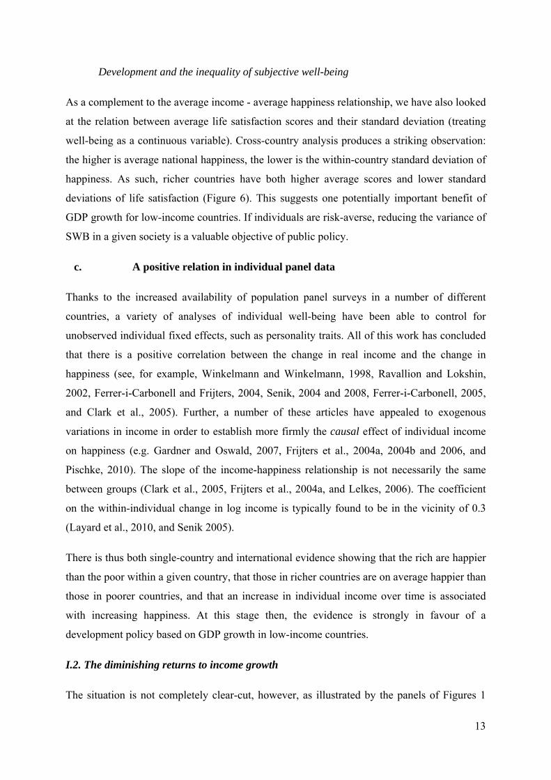
As a complement to the average income - average happiness relationship, we have also looked
at the relation between average life satisfaction scores and their standard deviation (treating
well-being as a continuous variable). Cross-country analysis produces a striking observation:
the higher is average national happiness, the lower is the within-country standard deviation of
happiness. As such, richer countries have both higher average scores and lower standard
deviations of life satisfaction (Figure 6). This suggests one potentially important benefit of
GDP growth for low-income countries. If individuals are risk-averse, reducing the variance of
SWB in a given society is a valuable objective of public policy.
c. A positive relation in individual panel data
Thanks to the increased availability of population panel surveys in a number of different
countries, a variety of analyses of individual well-being have been able to control for
unobserved individual fixed effects, such as personality traits. All of this work has concluded
that there is a positive correlation between the change in real income and the change in
happiness (see, for example, Winkelmann and Winkelmann, 1998, Ravallion and Lokshin,
2002, Ferrer-i-Carbonell and Frijters, 2004, Senik, 2004 and 2008, Ferrer-i-Carbonell, 2005,
and Clark et al., 2005). Further, a number of these articles have appealed to exogenous
variations in income in order to establish more firmly the causal effect of individual income
on happiness (e.g. Gardner and Oswald, 2007, Frijters et al., 2004a, 2004b and 2006, and
Pischke, 2010). The slope of the income-happiness relationship is not necessarily the same
between groups (Clark et al., 2005, Frijters et al., 2004a, and Lelkes, 2006). The coefficient
on the within-individual change in log income is typically found to be in the vicinity of 0.3
(Layard et al., 2010, and Senik 2005).
There is thus both single-country and international evidence showing that the rich are happier
than the poor within a given country, that those in richer countries are on average happier than
those in poorer countries, and that an increase in individual income over time is associated
with increasing happiness. At this stage then, the evidence is strongly in favour of a
development policy based on GDP growth in low-income countries.
I.2. The diminishing returns to income growth
The situation is not completely clear-cut, however, as illustrated by the panels of Figures 1
13

and 2: the positive relationship between income and happiness exhibits diminishing returns.
This comes as no surprise to economists, who are accustomed to the idea of the concavity of
preferences, i.e. decreasing marginal utility and risk-aversion. Concretely, this means that the
effect of earning an additional ten thousand dollars on subjective well-being becomes
progressively smaller as one’s initial level of income increases. This is consistent with the
good fit of the log functional form for income-happiness relationship, which is a familiar
result in the empirical analysis of subjective well-being across the social sciences.
a. Is there a threshold in the utility of growth?
“Once a country has over $15,000 per head, its level of happiness appears to be independent
of its income per head” (Layard, 2003, p. 17)
Many authors have suggested a threshold in the welfare effect of income. They recognize that
rich countries are happier than poor countries, but believe that there is no strong relationship
between GDP per capita and happiness among rich countries. This threshold separates
“survival societies” and “modern societies” (Inglehart et al., 2009). It is usually found to be in
an interval from US$10,000 to $15000 per annum (Di Tella et al., 2007).4 Layard (2005, p.
149) thus writes: “if we compare countries, there is no evidence that richer countries are
happier than poorer ones—so long as we confine ourselves to countries with incomes over
$15,000 per head.… At income levels below $15,000 per head things are different….”. Frey
and Stutzer (2002, p. 416) similarly claim that “income provides happiness at low levels of
development but once a threshold (around $10,000) is reached, the average income level in a
country has little effect on average subjective well-being”.
Even more explicitly, Inglehart (1997, pp. 64-65) concludes that: “the transition from a
society of starvation to a society of security brings a dramatic increase in subjective well-
4 This notion of a satiation point also goes back to Adam Smith’s concept of “a full complement of riches”,
beyond which there could be not be desire for more money. The large landholders of the 18th Century had
(according to him) reached this limit. However, there may be a limit to the quantity of wealth someone can enjoy
in a given society at a certain point of time, but this does not mean that this limit cannot be stretched by the set of
new choices brought about by economic growth (e.g. the internet). In other words, the “full complement of
riches” could be wider in richer than in less-developed countries.
14

being. But we find a threshold at which economic growth no longer seems to increase
subjective well being significantly. This may be linked with the fact that, at this level,
starvation is no longer a real concern for most people. Survival begins to be taken for granted
[…] At low levels of economic development, even modest economic gains bring a high return
in terms of caloric intake, clothing, shelter, medical care and ultimately in life expectancy
itself. […]. But once a society has reached a certain threshold of development … one reaches
a point at which further economic growth brings only minimal gains in both life expectancy
and subjective well-being. There is still a good deal of cross national variation, but from this
point on non-economic aspects of life become increasingly important influences on how long
and how well people live”… The authors continue to reach the same conclusion with updated
data: “Happiness and life satisfaction rise steeply as one moves from subsistence-level poverty
to a modest level of economic security and then levels off. Among the richest societies, further
increases in income are only weakly linked with higher levels of SWB” (Inglehart et al., 2008,
p. 268).
If true, the implication of these findings for developing countries is that GDP growth should
be seen as a temporary objective, to be retained only up to a certain level.
b. But the happiness-log GDP per capita gradient does not tend to zero.
In spite of these strong claims, the cross-country evidence in favour of such a subsistence
level is far from consensual. Bringing together a number of international survey datasets that
covering about 90% of the world’s population, including many developing countries (based
on the World Values Survey and the Gallup World Poll), Stevenson and Wolfers (2008, pp.
11-12) test for the idea of a cut-point at $15,000 per capita per annum (in constant 2000
dollars). They estimate the happiness-GDP per capita gradient, and find that: “the well-being-
GDP gradient is about twice as steep for poor countries as for rich countries. That is […] a
rise in income of $100 is associated with a rise in well-being for poor countries that is about
twice as large as for rich countries”. However, the marginal utility of GDP growth is still
positive in developed countries. “The point estimates are, on average, about three times as
large for those countries with incomes above $15,000 compared to those countries with
incomes below $15,000”. […] Taken at face value, the Gallup results suggest that a 1 percent
rise in GDP per capita would have about three times as large an effect on measured well-
being in rich as in poor nations. Of course, a 1 percent rise in U.S. GDP per capita is about
15

ten times as large as a 1 percent rise in Jamaican GDP per capita”.
This result is consistent with Deaton’s analysis of the same Gallup World Poll data (Figure
2.B): “the relationship between log per capita income and life satisfaction is close to linear.
The coefficient is 0.838, with a small standard error. A quadratic term in the log of income
has a positive coefficient: confirming that the slope is higher in the richer countries! […]
Using 12000$ of income per capita as a threshold between rich and poor countries shows
that the slope in the higher income countries is higher! […] If there is any evidence for a
deviation, it is small and is probably in the direction of the slope being higher in the high-
income countries”.
Deaton (2008) concludes that “the slope is steepest among the poorest countries, where the
income gains are associated with the largest increases in life satisfaction, but it remains
positive and substantial even among the rich countries; it is not true that there is some critical
level of GDP per capita above which income has no further effect on life satisfaction”. In
other words, there is indeed diminishing marginal utility to GDP growth, as the level of GDP
per capita increases, but the return to growth does not converge to zero.5
To summarize, an undisputed finding of the happiness literature based on cross-sections of
countries is that the relationship between income per capita and happiness is concave, i.e. has
diminishing returns. However, there is no consensus on the existence of a subsistence
threshold beyond which the marginal utility of income falls to zero.
1.3 “Rather than diminishing marginal utility of income, there is a zero marginal utility of
income”
The most powerful criticism of pro-growth policy hinges on the empirical evidence regarding
the within-country long-run changes in GDP and happiness. Visual evidence provided by
Easterlin and his co-authors (1974, 1995, 2005, 2007, 2009 and 2010) illustrates the flatness
of the long-run happiness curve plotted against time. One of the most famous and spectacular
5 It is worth underlying that while the log function is indeed concave, it is not bounded from above. If y=log(x),
then y does not tend to any fixed value as x tends to infinity. Yet, this is the message that a vast majority of
specialists in the field have drawn from the decreasing marginal utility of income and the good fit of the log-
linear functional form for the relationship between income and happiness.
16

of these flat curves is show in Figure 3.A, taken from Easterlin and Angelescu (2007). In spite
of the doubling of U.S. GDP per capita over a 30-year period (1972-2002), the average
happiness of Americans has remained constant. Average happiness is calculated using
repeated cross-sections from the American General Social Survey. The same type of pattern
has been uncovered in a number of other contributions, with long time-series data covering
different developed countries (see Diener and Oishi, 2000). The claim supported by these
graphs is radical: in the words of Richard Easterlin, “Rather than diminishing marginal utility
of income, there is a zero marginal utility of income” (Easterlin and Angelescu, 2007, p. 8).
The absence of any long-run correlation between growth and happiness could be explained by
the decreasing marginal utility of income uncovered in the cross-section. However, Easterlin
strongly rejects this interpretation: “The usual constancy of subjective well-being in the face
of rising GDP per capita has typically been reconciled with the cross-sectional evidence on
the grounds that the time series observations for developed nations correspond to the upper
income range of the cross-sectional studies, where happiness changes little or not al all as
real income rises.” But “the income change over time within the income range used in the
point-of-time studies do not generate the change in happiness implied by the cross-sectional
pattern”. (Easterlin and Angelescu, 2007, p. 24). For example: “in 1972, the cohort of 1941-
1950 had a mean per capita income of about 12000$ (expressed in 1994 constant prices). By
the year 2000, the cohort’s average income had more than doubled, rising to almost 27000$.
According to the cross-sectional relation, this increase should have raised the cohort’s mean
happiness from 2.17 to 2.27. In reality, the actual happiness of the cohort did not change”.
In some of his articles (Easterlin, 2005a, and Easterlin and Sawangfa 2005), Easterlin has
forcefully underlined that cross-section evidence cannot be transposed to the relationship over
time. The change in average self-reported happiness in a country, in the long-run, is not
correctly predicted by the instantaneous cross-section relationship between income per head
and happiness. Hence: “knowing the actual change over time in a country’s GDP per capita
and the multi-country cross-sectional relation of SWB to GDP per capita adds nothing, on
average, to one’s ability to predict the actual time-series change in SWB in a country”
(Easterlin and Sawangfa, 2009, p. 179). This is illustrated in Figure 3.B, taken from Easterlin
(2005a, p. 16), which contrasts the actual (flat) evolution of happiness in Japan, and the
predicted (log-linear) change over time.
17

Hence, the positive concave relationship between GDP per capita and SWB, observed in the
cross section, cannot be used to predict the change in SWB in developing countries over time.
This new “no bridge” theory underlines the “fallacy” of transposing cross-sectional relations
to time-series data. The lesson for developing countries is that they should not necessarily
expect to reach the higher level of well-being that is typical of developed countries by
growing over time.
I.4 Is the time-series correlation small enough to ignore?
In spite of the spectacular visual evidence offered by Easterlin, his rejection of any correlation
between over time between growth and happiness is still the object of vivid controversy. In
particular, one disputed point is whether the size of the correlation coefficient between SWB
and GDP per capita is statistically significant, and large. It is small, but is it “small enough to
ignore”? (Hagerty and Veenhoven, 2000, p. 4).
For instance, the absence of correlation between growth and happiness in the fast-developing
countries of Japan (after WWII) and China (after 1980) is particularly disappointing.
However, Stevenson and Wolfers (2008) have noted a number of discontinuities in the
wording of the happiness question and in the sampling of the Japanese cross-sections used by
Easterlin. With respect to China, the evidence is scarce (only three points in time) and
Hagerty and Veenhoven (2000) underline the fact that the Chinese sample is not
representative of the population, as it was initially biased towards more urban demographic
groups.
Other work on the long-run macroeconomic time series of happiness has concluded that there
is a positive relationship between growth in GDP per capita and well-being. Exploiting the
World Values Survey, Hagerty and Veenhoven (2003) found that GDP is positively related to
the number of “happy life years” in 14 of the 21 countries available in the dataset. In a later
paper, Hagerty and Veenhoven (2006) observed a statistically-significant rise in happiness in
4 out of 8 high-income countries, and 3 out of 4 low-income countries. Inglehart et al. (2008)
also exploited the most recent waves of the World Values Survey, spanning from 1981 to
2005. They found that, over the complete period, happiness rose in 45 out of the 52 countries
for which substantial time-series data is available. Kenny (2005) appeals to data on 21
Transition and Developed Countries and runs regressions of the change in happiness on the
growth in GDP, separately for each country. He finds that 88% of correlation coefficients are
18
positive; the overall regression coefficient for all countries together is positive and significant
at the 5% level.
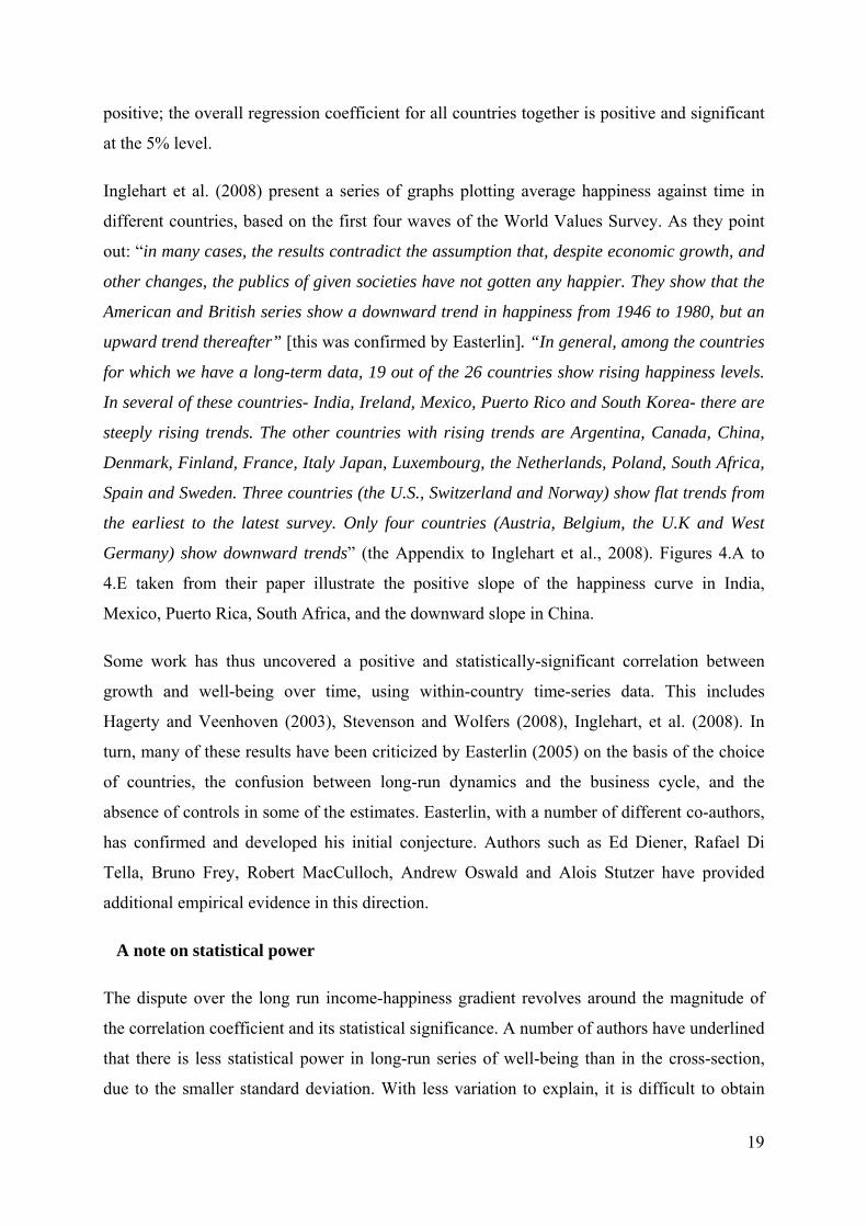
Inglehart et al. (2008) present a series of graphs plotting average happiness against time in
different countries, based on the first four waves of the World Values Survey. As they point
out: “in many cases, the results contradict the assumption that, despite economic growth, and
other changes, the publics of given societies have not gotten any happier. They show that the
American and British series show a downward trend in happiness from 1946 to 1980, but an
upward trend thereafter” [this was confirmed by Easterlin]. “In general, among the countries
for which we have a long-term data, 19 out of the 26 countries show rising happiness levels.
In several of these countries- India, Ireland, Mexico, Puerto Rico and South Korea- there are
steeply rising trends. The other countries with rising trends are Argentina, Canada, China,
Denmark, Finland, France, Italy Japan, Luxembourg, the Netherlands, Poland, South Africa,
Spain and Sweden. Three countries (the U.S., Switzerland and Norway) show flat trends from
the earliest to the latest survey. Only four countries (Austria, Belgium, the U.K and West
Germany) show downward trends” (the Appendix to Inglehart et al., 2008). Figures 4.A to
4.E taken from their paper illustrate the positive slope of the happiness curve in India,
Mexico, Puerto Rica, South Africa, and the downward slope in China.
Some work has thus uncovered a positive and statistically-significant correlation between
growth and well-being over time, using within-country time-series data. This includes
Hagerty and Veenhoven (2003), Stevenson and Wolfers (2008), Inglehart, et al. (2008). In
turn, many of these results have been criticized by Easterlin (2005) on the basis of the choice
of countries, the confusion between long-run dynamics and the business cycle, and the
absence of controls in some of the estimates. Easterlin, with a number of different co-authors,
has confirmed and developed his initial conjecture. Authors such as Ed Diener, Rafael Di
Tella, Bruno Frey, Robert MacCulloch, Andrew Oswald and Alois Stutzer have provided
additional empirical evidence in this direction.
A note on statistical power
The dispute over the long run income-happiness gradient revolves around the magnitude of
the correlation coefficient and its statistical significance. A number of authors have underlined
that there is less statistical power in long-run series of well-being than in the cross-section,
due to the smaller standard deviation. With less variation to explain, it is difficult to obtain
19

statistically-significant correlations.
Hagerty and Veenhoven (2000, p. 5) for instance, note that: “the standard deviation in GDP
per capita in the cross section from Diener and Oishi was about 8000$, whereas the standard
deviation in Hagerty time-series (for the same countries) was only about ¼ of that (2000$)
[…] within a country in 25 years”. Hence, the statistical power to detect the effect is lower in
time-series work. Equally, Kenny (2005), using data on 21 Transition and developed
countries, found a standard deviation in happiness over time within countries of 0.28 on
average, as compared to a standard deviation of average scores across countries of 0.65 (p.
212). Layard et al. (2010, p. 161), using Eurobarometer time series for 20 Western European
countries, also report an average standard deviation of national happiness scores over time of
0.2, as compared to an average of 0.5-0.6 in the individual cross-sections.
We calculated the standard deviation in happiness and life satisfaction in the World Values
Survey cross-sections from 1981 to 2007. The average standard deviation within a cross-
section (250 observations) is 0.67 for happiness (4-point scale) and 2.14 for life satisfaction
(10-point scale). But the standard deviation of average national happiness across countries is
0.28 for happiness and 1.04 for life satisfaction. Finally, the standard deviation of national
happiness over time fluctuates around 0.1 for happiness and from 0.13 to 0.41 for life
satisfaction. In other words, the variability of subjective well-being measures is much lower in
time-series than in the cross-sections within countries and across-countries. The implication is
that the difference between cross-sectional versus time-series correlation coefficients is
difficult to interpret.
In summary, the long-run relationship between GDP growth and subjective well-being is still
a subject of some controversy. As pointed by Stevenson and Wolfers (2008), one cannot
reject the null that the correlation coefficient is equal to zero, but this does not mean that one
can reject the null that it is greater than zero. The nature of the long-run relationship between
GDP and well-being is far from being firmly established.
I.5 Subjective well-being and the business cycle
One of the reasons why it is difficult to admit no correlation between income and well-being
is that this appears in sharp contradiction to the undisputed welfare effect of the business
cycle.
20

There is first of all considerable consensus that recessions make people unhappy. Di Tella et
al. (2003) showed that macroeconomic movements, in particular unemployment, inflation and
the volatility of output exert strong effects on the happiness of nations. The negative impact of
volatility on subjective well-being was also established by Wolfers (2003). A powerful
illustration of the business cycle-happiness correlation is given in Figure 5.A, taken from
Stevenson and Wolfers (2008), which shows the spectacular parallel dynamics of the output
gap and the average happiness in the United States from 1972 to 2008. This does not mean
that the influence of the business cycle can be equated with the influence of long-run growth,
however. It is indeed easy to imagine happiness and the business cycle fluctuating around a
flat long-run trend. While it is uncontroversial to say that happiness rises in booms and falls in
busts, the key question is whether four percent growth in GDP per annum (for example) will
produce a happier society in the long run than one percent GDP growth per annum.
One particular episode which is often considered as an illustration of the correlation between
income fluctuations and well-being, rather than between long-term growth and well-being, is
the transition process in Central and Eastern European countries from socialism to capitalism.
All of the work here recognizes the statistically-significant correlation between the dynamics
of GDP and that of subjective well-being. Figures 5.B to 5.D, taken from Guriev and
Zhuravskaya (2008) and Easterlin (2009), illustrate the concomitant evolutions in income and
happiness in a number of transition countries. Similar evidence can be found in Sanfey and
Teksoz (2008).
However, these trends are qualified as short term by Easterlin and Angelescu (2009), who
warns that one should avoid “confusing a short-term positive happiness-income association,
due to fluctuations in macroeconomic conditions, with the long-term relationship. We suggest,
speculatively, that this disparity between the short and long-term association is due to the
social psychological phenomenon of “loss aversion”.
However valuable the interpretation in terms of loss-aversion, it is perhaps surprising that
Transition is considered to be only a short-term phenomenon. In a way, Transition is the best
example of regime change that we can think of. It is a deep and irreversible structural
transformation, not a short-lived phenomenon. It shares the essential features of development,
including the take-off period and the profound qualitative and institutional changes. Hence,
whether Transition should be treated as a short-term or a long-term phenomenon remains an
open question. Only the passage of time will enable us to see whether the increase in
21

subjective well-being continues with GDP growth, stagnates at a certain point, or falls back
down to the initial (1990) level.
II. EXPLANATIONS RELATED TO GROWTH ITSELF: CHANNELS AND
NEGATIVE SIDE-EFFECTS
The flatness of happiness curves is therefore consistent with GDP growth not yielding higher
well-being over time. More generally, it may suggest that whatever changes a country
experiences over time have no long-run effect on individual average happiness. If this is true,
the prospect is dark for developing countries, which are locked in at their current low level of
happiness. The message is also very discouraging for public policy in general: if happiness
cannot be raised in the long run, not only should growth be abandoned as an objective, but so
should any other public policy measure.
Before jumping to these radical conclusions, the two next sections discuss possible
explanations of the flatness of the happiness curve. A first series of explanations pertain to the
nature of growth itself, i.e. the channels of growth and the fact that growth is accompanied by
negative externalities (pollution, inequality etc.) that cancel out its subjective benefits. The
second series of explanations cover social and psychological processes, such as comparisons
and adaptation, that may well reduce the happiness benefits of growth.
II.1 Quality of Life: channels from GDP growth to happiness
Statistical estimates of subjective well-being most often include time and/or country fixed
effects, as well as other controls that are introduced in order to pick up any changes in the
demographic composition of the population (in terms of age, occupation, health, number of
children, etc.). Some analyses also control for political variables such as democracy, gender
equality, trust, etc. However, in terms of the empirical strategy retained for the estimation of
the relationship, there is always a trade-off between controlling for variables that reflect the
channels via which the phenomenon under consideration works, and not controlling for
omitted variables and obtaining a biased measure of the relationship. For example, in the
context of the current question of growth and well-being, a well-being regression that
controlled for both GDP and the positive side-effects (or channels) of growth runs the risk of
concluding that growth doesn’t matter for well-being. Indeed, we expect growth to bring
about higher well-being not only via greater purchasing power (income), i.e. through higher
22
consumption, but also via other transformations (education, health etc.) which accompany the
growth process. Controlling for these latter transformations may render GDP itself
insignificant in a well-being equation, but that does not mean that greater income does not
produce greater happiness, it rather means that we have identified the different processes via
which income produces well-being.
Greater income per capita always comes with increased labour productivity, which means a
greater choice in time-use for those who are concerned. As argued by Sen (2001), it is
because it enhances the freedom of choice (by enlarging their set of capacities) that growth is
expected to raise people’s well-being. Identically, GDP growth is known for being associated
with demographic transitions in developing countries. This is certainly “a revolutionary
enlargement of freedom for women”, as put by Titmuss (1966, quoted by Easterlin and
Angelescu 2007, p. 9), and a rise in the education and resources for self-development that
children can count on. Growth also comes with higher life expectancy, reduced child
mortality and child underweight (see for instance Becker, Philipson and Soares, 2005 and
Easterlin and Angelescu, 2007). Finally it is well-known that democracy and development go
hand in hand, even if the direction of causality is not as clear as was believed in the 18th
Century (e.g. by Montesquieu, Steuart and Hume). Lipset (1959, p. 80), for example, claims
that: “industrialization, urbanization, high educational standards and a steady increase in the
overall wealth of society [are] basic conditions sustaining democracy”. Without inferring any
causality, we can observe the statistical association between GDP growth and progress in
terms of political freedom and human rights. With respect to the empirical strategy, any
attempt to capture the global effect of GDP growth on subjective well-being should not
control for any such variables which represent the channels of transmission. It is likely
regrettable that much of the work on the GDP growth-happiness relationship does indeed
include such controls.
The following sections review the available evidence on the correlation between GDP growth
and such quality of life indicators. These latter are measures of the non-income quantitative
and qualitative dimensions that constitute the channels from income growth to well-being.
a. Cross-section correlation between GDP growth and Quality of Life indicators
Easterlin and Angelescu (2007) illustrate the sizeable positive correlation in cross-section data
between a number of quality of life indicators and GDP per capita across countries at different
23

levels of development. The clear upward slopes relate subjective well-being to quantifiable
factors, measured on continuous scales. These latter include food, shelter, clothing and
footwear, energy intake, protein intake, fruit and vegetables, radios, cars, TV sets, mobile
phone subscriptions, internet users, urban population, life expectancy at birth, gross education
enrolment rate, and the total fertility rate. These kinds of relationships have been documented
by a considerable number of other authors, including Inglehart and Welzel (2005), Inglehart et
al. (2008), Layard et al., 2010, Di Tella and MacCulloch (2008), and Becker et al. (2005).
Along analogous lines, some authors have insisted on the relationship between subjective
well-being, on the one hand, and procedures, governance and institutions, democratic and
human rights, tolerance of out-groups, gender equality, on the other (for example, Barro 1997,
Frey and Stutzer 2000, Inglehart and Welzel 2005, Schyns 1998, and Inglehart et al. 2008).
b. Time-series correlation between GDP growth and Quality of Life indicators
Figure 7 illustrates the spectacular take-off of life expectancy in England and Wales in the
19th century. More generally, Easterlin and Angelescu (2007) provide a detailed account of
the progress in the different dimensions of quality of life over time, in a large set of developed
and emerging countries. They document the different dimensions of changes in the Quality of
Life during “modern economic growth”. The latter is defined as a “rapid and sustained rise in
real output per head and attendant shifts in production technology, factor input requirements,
and the resource allocation of a nation”, where “rapid and sustained” is defined as being
equal to at least 1.5% per year (Easterlin and Angelescu, 2007, p. 2).
Easterlin and Angelescu document the turning points in GDP growth and other indicators of
the Quality of Life. Although both variables move in parallel, they insist that the dates of their
respective take-offs do not systematically coincide. Qualitative indicators sometimes lag
behind and sometimes are lead the date of GDP take-off. “If social and political indicators of
QoL are, at present, positively associated with GDP per capita, it is often because the
countries that first implemented the new production technology underlying modern economic
growth were also the first to introduce, often via public policy, new advances in knowledge in
the social and political realms” (Easterlin and Angelescu, 2007, p. 21). Whether the co-
movements between growth and quality of life indicators represent a causal relationship is
controversial and difficult to establish (see also Easterly, 1999). However, it is undeniable that
24

overall there is no progress in quality of life without GDP growth.
In their provocative paper “Is growth obsolete?”, William Nordhaus and James Tobin (1973)
advocated for an alternative indicator, integrating leisure, household work, costs of
urbanization, and constructed a “Measure of Economic Welfare”. However, this index turned
out to grow in a way that was similar to GDP over the period under study, albeit more slowly.
This, to our knowledge is a universal observation. Pritchett and Summers (1996), for example,
note that “wealthier is healthier” in the long run. Using time-series data from a variety of
countries, they find that “The long-run income elasticity of infant and child mortality in
developing countries lies between 0.2 and 0.4”. This implies that “over a half a million child
deaths in the developing world in 1990 alone can be attributed to the poor economic
performance in the 1980s”.
In summary, GDP growth goes hand-in-hand with a series of quantitative and qualitative non-
monetary improvements in quality of life. These constitute the channels from growth to well-
being that we argue should not be controlled for in the statistical analysis of the former
relationship.
II. 2. Negative side-effects of growth
The flatness of the GDP-happiness graphs may be due to the negative influence of some side-
effects of growth, such as pollution, income inequality, work stress, and so on. The influence
of these “omitted variables” could then well hide the positive influence of GDP growth on
subjective well-being in econometric analyses (see Di Tella and MacCulloch, 2008).
The most widely-discussed negative side-effects of growth are: inequality, crime, corruption,
extended working hours, unemployment, pollution and other environmental degradation (as
measured by SOx emissions, for example). These are discussed in Di Tella and MacCulloch
(2003 and 2008). Kenny (2005) also emphasises the social cost of economic transformation,
and the ensuing shift from local to global relative income concerns. The impact of urban
concentration and sub-urbanization is not so clear-cut, however. Easterlin and Angelescu
(2007) also underline the effects of carbon dioxide emissions and fat intake (obesity and
blood pressure). Clark and Fischer (2009) provide a useful summary of the macro-economic
correlates of life satisfaction in OECD countries.
Among the list of usual suspects, income inequality occupies a particular place. In the first
25
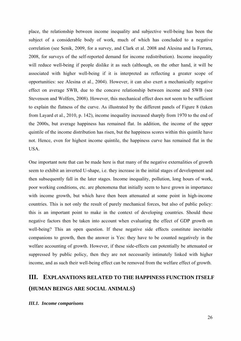
place, the relationship between income inequality and subjective well-being has been the
subject of a considerable body of work, much of which has concluded to a negative
correlation (see Senik, 2009, for a survey, and Clark et al. 2008 and Alesina and la Ferrara,
2008, for surveys of the self-reported demand for income redistribution). Income inequality
will reduce well-being if people dislike it as such (although, on the other hand, it will be
associated with higher well-being if it is interpreted as reflecting a greater scope of
opportunities: see Alesina et al., 2004). However, it can also exert a mechanically negative
effect on average SWB, due to the concave relationship between income and SWB (see
Stevenson and Wolfers, 2008). However, this mechanical effect does not seem to be sufficient
to explain the flatness of the curve. As illustrated by the different panels of Figure 8 (taken
from Layard et al., 2010, p. 142), income inequality increased sharply from 1970 to the end of
the 2000s, but average happiness has remained flat. In addition, the income of the upper
quintile of the income distribution has risen, but the happiness scores within this quintile have
not. Hence, even for highest income quintile, the happiness curve has remained flat in the
USA.
One important note that can be made here is that many of the negative externalities of growth
seem to exhibit an inverted U-shape, i.e. they increase in the initial stages of development and
then subsequently fall in the later stages. Income inequality, pollution, long hours of work,
poor working conditions, etc. are phenomena that initially seem to have grown in importance
with income growth, but which have then been attenuated at some point in high-income
countries. This is not only the result of purely mechanical forces, but also of public policy:
this is an important point to make in the context of developing countries. Should these
negative factors then be taken into account when evaluating the effect of GDP growth on
well-being? This an open question. If these negative side effects constitute inevitable
companions to growth, then the answer is Yes: they have to be counted negatively in the
welfare accounting of growth. However, if these side-effects can potentially be attenuated or
suppressed by public policy, then they are not necessarily intimately linked with higher
income, and as such their well-being effect can be removed from the welfare effect of growth.
III. EXPLANATIONS RELATED TO THE HAPPINESS FUNCTION ITSELF
(HUMAN BEINGS ARE SOCIAL ANIMALS)
III.1. Income comparisons
26

One simple explanation of the lack of any long-run relationship between income and well-
being is that this does not reflect that there is something wrong with growth per se, but rather
that this reflects the very structure of individual well-being functions. The broad idea is that
income does not bring well-being in a vacuum, but is rather intensely social, in that it is
evaluated relative to some benchmark, reference or comparison level of income. There are
many synonyms for the latter: this can be thought of as what is normal in the society, or what
is fair. Forgetting about the other determinants, we can then write the relationship between
utility and income as:
Uit = U(yit, yit*) (1)
The well-being of individual i at time t rises with their own income, yit, but falls with the level
of comparison income, yit*. Comparison income acts as a deflator with respect to own income
here, in the sense that the higher it is the less good the individual’s own income looks. Much
of the empirical literature exploring this relationship has explicitly parameterized the well-
being function as a function of both yit, and yit/yit*. If the income effect of income on well-
being is mostly absolute, so that absent the externalities mentioned above greater GDP will
increase individual well-being, then the second term will play only a minor role. On the other
hand, if income comparisons are very important, so that most of the effect of income works
through how well I am doing compared to some reference group, then it is the second term
that will be preponderant. If it is mostly relative income (yit/yit*, which is homogeneous of
degree zero) that matters, then, answering Dick Easterlin’s 1995 question, Raising the
Incomes of All will not Increase the Happiness of All.
Distinguishing between these two scenarios has been the goal of a considerable amount of
empirical work over the past fifteen or so years. A variety of different empirical approaches
across various disciplines have been mobilized to answer the question of how much income
comparisons matter in the determination of well-being. All of this work has had to set out a
priori exactly to whom or to what individuals are thought to compare themselves: this has
included the individual’s spouse, to people with the same characteristics as the individual,
those in the same region, other participants in experiments, hypothetical individuals, or even a
measure of the individual’s expected income. Some of the key findings in developed countries
are described below.
27

a. Evidence in Developed Countries
One direct approach to the question of income comparisons has been to estimate well-being
regressions in which both the individual’s own income and the comparison income level
appear: these are the empirical counterpart to equation (1) above. This literature has appealed
to different datasets (in terms of countries and years), different measures of well-being (job
and life satisfaction being the most predominant), and various measures of comparison
income, yit*. The typical finding is that own income is positively correlated with well-being,
but that the correlation with others’ income is negative.
Clark and Oswald (1996) use the BHPS to calculate the income of ‘people like me’ from a
wage equation, and show that this is negatively correlated with individual job satisfaction.
Own income attracts a positive coefficient, and the sum of the two estimated income
coefficients is zero: pay rises for everyone have no effect on satisfaction. More recent work
along the same lines using, respectively, German and American data is Ferrer-i-Carbonell
(2005) and McBride (2001). Vendrik and Woltjer (2006) extend the analysis of the German
GSOEP data in this respect, by considering asymmetric reactions to gains and losses (relative
to the reference group).
An alternative measure of yit* is at the local level: What do my neighbours earn? Both
Blanchflower and Oswald (2004) and Luttmer (2005) calculate regional average income in
US data, and show that this is negatively correlated with respondents’ well-being: an
individual earning $40 000 per year is happier in a poorer than a richer region. However, at
the very local level of a few hundred metres, Clark et al. (2009) find that in Danish panel data,
conditional on my own income and local median income, my satisfaction is strongly
positively correlated with my rank in the local income distribution. Other work here has
considered comparisons to the income of the individual’s work colleagues (Brown et al.,
2006), partner (Clark, 1996) and parents (McBride, 2001).
Running well-being regressions is only one way of addressing the question of income
comparisons. One early method (the first published contribution being Van Praag, 1971) is
that of the Welfare Function of Income. Here individuals assign income levels (per period) to
verbal labels (such as excellent, good, sufficient and bad): these stated values form the basis
of individual-level regressions estimating a lognormal Welfare Function of Income. The
resulting individual estimated means (μ) reveal which individuals require greater income in
28

order to be satisfied. Comparison income is introduced into the analysis, typically as average
income over age, education and other characteristics. The regression results (for example, Van
de Stadt et al., 1985) show that, given own income, the higher is reference group income, the
more money individuals say they need to reach a given verbal well-being level, which is
consistent with income comparisons.
Separate evidence on comparisons is found in experimental economics. In Zizzo and Oswald
(2001), experimental participants paid out of their own winnings in order to burn the money
earned by other participants. An alternative approach is to ask individuals to choose between
hypothetical outcomes, as in Alpizar et al. (2005), Johannsson-Stenman et al. (2002) and
Solnick and Hemenway (1998). A typical income choice is as follows:
A: Your current yearly income is $50,000; others earn $25,000.
B: Your current yearly income is $100,000; others earn $200,000.
The key here is that one choice has a greater absolute return while the other is more
advantageous in relative terms. In line with the experimental work, there are strong positional
concerns over income, in that individuals choose A over B. While the above example is
couched in terms of income, the same method can be used to compare the degree of
comparisons across domains. For example, relative concerns in Alpizar et al. are stronger for
cars and housing, and weaker for vacations and insurance.
A recent randomized experiment was set up by Card et al. (2010), showing evidence of
relative concerns among employees of the University of California when they had access to
internet information about the wage of their colleagues.
Last, we can appeal to recent neurological work. Fließbach et al. (2007) use MRI techniques
to measure the brain activity of pairs of individuals engaged in identical guessing-game tasks.
Each individual’s monetary reward for a correct guess was announced to both subjects, and
these rewards were varied. In some conditions a correct guess by a participant earned 60
points; in other conditions the subject’s guess earned 60 and the other’s correct guess earned
30, or 60 and 120. As such, the individual’s relative payoff for a correct guess changed, while
keeping the absolute reward fixed. Blood oxygenation analysis showed that brain activity in
the ventral striatum was increased with relative income. Related work in this area appears in
29

Takahashi et al. (2009).
b. Evidence in LDCs
The majority of the work on income comparisons and individual well-being has covered
OECD countries. However, the increasing availability of data including subjective questions
undoubtedly allied with the increasing interest that researchers have in these issues, have
produced a small but growing number of pieces of evidence regarding the correlates of
individual well-being in poorer countries. The key question that we want to answer here is
whether positional concerns are less important in poorer countries: Are comparisons luxuries?
Regarding the direct estimation of individual well-being, Graham and Felton (2006) have
replicated the finding of a negative effect of regional income on individual well-being across
18 Latin American countries. Kuegler (2009) analyzes self-collected data on 400 Venezuelans
in 2005, and shows that those who say that they are better off than their own siblings report
higher life satisfaction. This is consistent with relative income effects in a relatively poor
country. The strength of this correlation depends on the individual’s own characteristics,
being stronger for respondents with above-median incomes and those who work in higher-
rank professions. Stark and Taylor (1991) present indirect evidence of the role of income
comparisons by looking at the decision to migrate. Using Mexican data, they show that
relative deprivation is a significant predictor of Mexico-US migration.
Castilla (2010) also considers Mexican data, including information on subjective poverty
(whether the respondent’s income is sufficient for their needs) and income satisfaction.
Relative concerns are introduced by considering these two welfare measures as a function of
both own expenditure and the respondent’s evaluation of their own income relative to people
with whom they live, to how much they aspired to have at this stage of their lives, and relative
to the income they earned three years ago (all three of which are measured on a seven-point
scale). The empirical results show that welfare rises with own expenditure, but falls with
income relative to others and income relative to aspirations. The results with respect to past
income are significant only in the life satisfaction equation and when the individual reports
being worse off than three years ago (which is consistent with loss-aversion).
Rojas and Jiménez (2007) also appeal to Mexican data to show respondents’ subjective
poverty evaluations are partly determined by the gaps between own income on the one hand
30

and comparison and aspired income levels on the other. Comparison income is measured
directly by asking about the income gap ‘with respect to those you usually compare yourself
to’. Guillen-Royo (2010) analyzes small sample data from seven communities in Peru, and
shows that satisfaction with a number of different life domains is positively correlated with
own expenditure but negatively correlated with average community expenditure. Last, Rojas
(2010) uses data from 20 Latin American countries found in the 2007 Gallup survey. Two
measures of individual well-being, the ladder question of worst to best possible life and
satisfaction with standard of living, are related to both own income and the average income in
the reference group (defined by age, sex and country). The empirical results show that well-
being rises with the log of own income but falls with the log of comparison income. In the
case of satisfaction with standard of living, the coefficients on the two variables are equal and
opposite, suggesting that a rise in everyone’s income would leave no-one in Latin America
better off.
Moving from Latin America to Asia, there has been a spate of recent work on the
determinants of well-being in China, some of which has appealed to the notion of reference
income. Appleton and Song (2008) conclude that the life satisfaction reported by urban
Chinese is affected by status considerations, and Smyth and Qian (2008) analyze data from 31
Chinese cities in September 2002, finding that the log of average monthly income in the city
in which the respondent lives is negatively correlated with happiness, controlling for own
income. Gao and Smyth (2010) appeal to two different datasets to present some evidence that
job satisfaction is negatively related to reference group income, where this latter is either
average income in the firm in which the respondent works, or the predicted income of “people
like me” (as in Clark and Oswald, 1996).
Recent work by Cojocaru (2010) appeals to cross-section 2007 data from the LSMS in
Tajikstan. He finds a mostly insignificant effect of regional income on individual life
satisfaction, but suggests that this might reflect the fact that the wrong reference group is
being used. When however a qualitative variable is used which measures the individual’s
evaluation of their household’s welfare relative to that of their neighbours, strong effects are
found in the expected sense: those who rank their household relatively lowly compared to
their neighbours report lower levels of life satisfaction, controlling for the household’s own
expenditure.
31

Fafchamps and Shilpi (2008) consider a direct measure of relative utility in a developing
country by analysing the answers to a question on consumption adequacy in Nepalese data.
Consumption adequacy rises with own income (but falls with the distance to the nearest
market). Critically, conditional on these and other control variables, consumption adequacy
also falls with reference group consumption, as in a relative utility model. Here reference
group consumption is defined in a geographical way as the mean or median consumption of
other households living in the same ward as the respondent.
Carlsson et al. (2009) look at hypothetical preferences over different absolute and relative
income situations (as used by Alpizar et al., 2005) in India. They find that around half of the
effect of income on well-being comes from some kind of status or relative income concern.
Crucially, they note that this figure is around the same as that found in rich countries. They
moreover note that low caste and low income respondents seem to be more sensitive to
relative income.
John Knight has authored a series of papers using Chinese data from the 2002 CHIP national
household survey. Unusually, this survey included not only questions on subjective well-
being but also asked direct questions about who individuals considered as their reference
group. Knight et al. (2009) appeal to cross-sectional information on 9,200 households in
China. The authors first show that comparisons in China are local, in that 70% of individuals
see their village as their reference group. Further, conditional on both own and village
income, those who report that their own income was much above the village have higher
happiness scores. Knight and Gunatilaka (2010a and 2010b) also emphasize the importance of
relative income rather than absolute income, and the role of changing reference groups, in
Chinese data. Mishra et al. (2010) show that reporting an income below that of a self-reported
reference group is associated with lower well-being for the Korean minority in China.
Well-being work using Chinese data has thus uncovered a number of pieces of evidence
consistent with the presence of income comparisons in a developing country. This is
consistent with the results in Brown et al. (2010), who do not measure well-being directly, but
instead appeal to the literature that has analyzed conspicuous consumption in developing
countries. They use data from a Chinese household panel, and show that spending on funerals
and gifts is consistent with status-seeking behaviour. Last, Fließbach and co-authors followed
up their 2007 work by running the same relative income Neuro experiments in China
32

(although the results have not yet been written up).
Turning to Africa, Kingdon and Knight (2007) consider the role of relative income in South
Africa. The authors find evidence of negative relative income effects within race groups
(whereby life satisfaction is lower the more others earn), but positive relative income effects
within neighborhoods.6
Bookwalter and Dalenberg (2010) analyze South African SALDRU data from the early
1990s. They find no significant effect of local (cluster-level) income for Whites, but a positive
and significant effect of others’ income for non-Whites. However, similar to Cojocaru (2010),
dummy variables for one’s own income compared to that of one’s parents attract significant
estimated coefficients consistent with income comparisons (with feeling less well-off than
one’s parents having a far larger absolute effect on satisfaction than feeling better-off than
one’s parents).
Ravallion and Lokshin (2010) appeal to large-scale 2004 household data from Malawi, which
includes measures of satisfaction with life and consumption expenditure. More unusually, the
data also includes measures of own subjective economic welfare, from respondents’ answers
to the question “Imagine six steps, where on the bottom, the first step, stand the poorest
people, and on the highest step, the sixth, stand the rich (show a picture of the steps). On
which step are you today?”, as well as their assessment of the economic welfare of their
neighbors and their friends. Ravallion and Lokshin model individual life satisfaction as a
function of both own and local neighbourhood consumption, and as a function of both own
and others’ economic welfare. Although they argue that the results show that comparisons are
not important for the majority of Malawians, others’ consumption reduces individual life
satisfaction in the urban sample, and there is some evidence of a negative effect of friends’
economic welfare on those who report a relatively high level of own economic welfare.
On a smaller scale, Kenny (2005) uses data from a survey of 566 Tanzanian households, in
which respondents report the amount of income necessary to be wealthy. Similar to the
European results in Van Praag’s work, it is shown that the average income in the area is one
key determinant of what people consider to be a healthy income.
6 So that higher neighbourhood income is associated with greater satisfaction. This mirrors the finding in Danish small neighbourhood data in Clark et al. (2009). 33
Akay and Martinsson (2008) use a cell-mean approach similar to that in Ferrer-i-Carbonell
(2005) applied to 2004-2005 household survey data in Northern Ethiopia. They find no
significant effect of reference group income on life satisfaction. A companion paper (Akay et
al., 2009) again looks at Ethiopia, but this time considers hypothetical preferences over
absolute and relative income scenarios. The results here are that the choices of most Ethiopian
subsistence farmers are based on absolute income alone. However, there are still an arguably
considerable number of some of the poorest people in the world who take status
considerations into account. Corazzini et al. (2010) use the same approach to compare the
degree of relative income concerns across eight different countries. While they argue that
there is a broad pattern of individuals in richer countries being more sensitive to relative
income, it is striking that one of the most comparison-conscious countries in this respect is
Kenya.
c. Absolute versus relative poverty
One of the reasons why we are interested in income comparisons, especially in the context of
less well-off countries, is that they impinge on the concept of poverty. The distinction
between poverty as an absolute lack and a relative lack goes back at least to Adam Smith: in
the mid-18th Century the Scots were not seriously deprived if they did not have shoes,
whereas in England, only the truly destitute had no shoes. The stigma from being shoeless
was therefore greater in England than in Scotland, because of the social norm that was
attached to it. As such, the impact of a given lack on individual well-being may depend on the
degree to which this lack is stigmatised in society, which itself is likely related to the
incidence of the lack under consideration.
Moving back to income and appealing to equation (1) above, the critical distinction is then
whether poverty is defined by an individual’s income falling below a certain critical level, or
whether other people’s outcomes play a role. Absolute measures of poverty include the cost of
minimum calorie intake line, the minimum consumption basket defining the poverty line in
the US, and the World Bank’s 1$ a day poverty line. Relative measures of poverty take
context into account, such as the commonly-used relative poverty line set at 60% of median
income. The evidence of relative income concerns in low-income countries seems to
constitute an argument in favor of measures of relative poverty.
Another important question that we are unable to answer to date, is whether relative concerns
34

are less important, i.e. have smaller welfare effect in low-income countries than in high-
income countries. Income interactions can be thought about as some kind of luxury good, that
come into attention only once survival is taken for granted. We have reviewed the evidence
that relative concerns do exist in developing countries. But whether their importance is
smaller than in developed countries remains an open question that would need specific data –
maybe experimental data- to be answered. Analyzing the data from the third wave of the
European Social Survey, Clark and Senik (2010) focused on the answers to the question “How
important is it to you to compare your income with other people’s incomes?” across European
countries. They found that this importance is greater in poorer countries than in richer
countries, and that, within countries, this comparison is more often said to be important by
poorer people. Comparisons are most often upward directed and people suffer more from
upward-directed comparisons. This is consistent with the literature’s general findings (see for
example Ferrer-i-Carbonnell 2004, or Card et al. 2010). If this finding could be extended to
poor countries, this would rule out the idea that income comparisons are a rich country
phenomenon.
Knowing that local income comparisons matter for low-income countries’ citizens, one
should consider the possibility that global income concerns may also be important, especially
in view of the development of information and communication technologies. If the latter
allow the inhabitants of low-income countries to be aware of the life-style and consumption
possibilities of high-income country citizens, this is likely to generate feelings of relative
deprivation. This might explain the steeper curve of the relation between GDP per capita and
subjective well-being in developing countries (see section I.1). We are not aware of any direct
evidence of global income concerns. One exception is Clark and Senik (2010), who noted
that in the above-cited recent survey of Europeans, respondents who did not have internet
access were less subject to income comparisons.
The most radical view about the importance of income comparisons would lead to the
conclusion that it is only because they compare to others that the richer inhabitants of the
globe are more happy and the poorer less happy. Does this mean that low-income countries
should give up pro-growth policy? This would be surprising policy advice. Indeed, if relative
concerns are important, many may well find it strange to recommend that low-income
countries should remain at their current low rank in the concert of nations. Even if income
comparisons lead to a vain zero-sum rat race between countries, it is not clear that not
35

competing is an avenue for happiness.
III.2. Adaptation
Adaptation and the associated “hedonic treadmill” is another classic explanation of the
Easterlin paradox. Habituation effects destroy the welfare benefit of growth. This is because
of the deleterious role of aspirations: “Material aspirations increase commensurately with
income, and as a result, one gets no nearer to or farther away from the attainment of one’s
material goals, and well-being is unchanged” (Easterlin, 2003).
Adaptation is a central issue in the social sciences: to what extent do we get used to any
specific life situation? The psychological basis of adaptation is that judgements of current
situations depend on the experience of similar situations in the past, so that higher levels of
past experience may offset higher current levels of these phenomena due to changing
expectations (see Kahneman and Tversky, 1979). Some psychologists draw a parallel between
the homeostasis that leads us to hold body temperature steady and homeostasis in subjective
wellbeing (Cummins, 2003), which latter is argued to hold well-being at some constant
individual-specific set-point (argued to be between 60 and 80 on a standardised 0-100 scale,
with an average figure of 75). This may be partly biologically determined, underlying a
potential role of genetic factors. In any case, the key element is that, although positive and
negative events will have short-run effects on well-being, in the longer-run most individuals
will return to their set-point level.
Although initially partisans of the adaptation hypothesis, Fujita and Diener (2005) note that in
17 years of GSOEP data, around one quarter of people changed well-being significantly from
the first five to the last five years. Diener et al. (2006) propose 5 significant revisions to
hedonic-treadmill theory: 1) individuals’ set-points are not hedonically neutral; 2) individuals
have different set-points; 3) a single person can have multiple set-points depending on the
components of happiness (emotions, life satisfaction); 4) well-being set-points can change
under some conditions, 5) individuals differ in their adaptation to events.
In the context of the Easterlin paradox, we are particularly interested in adaptation to income.
With respect to equation (1) above, we again introduce an additional income term into the
utility function; however, this time the newcomer is not the income of others or expectations,
but rather the income that the individual themselves had earned in the past. Individual well-
36
being is thus still subject to income comparisons, but here the comparisons are within subject,
to use the psychological term. Those who have earned more in the past are less satisfied with
any given level of income today.
While in theory any past income level could negatively affect well-being today, in practice
empirical work has appealed to the income that the individual received one year ago (in panel
terms, this is the income that the individual reported in the previous wave, as most panels are
carried out on a yearly basis).
Uit = U(yit, yit-1) (2)
This kind of utility function implies that any attempt to raise happiness via higher income is
potentially subject to debate. If the effect (negative) of past income, via habituation, is strong
enough then income will have no long-lasting well-being effect, at both the individual and the
societal level.
a. Evidence in Developed Countries
Perhaps the best-cited piece of work in the domain of adaptation to income is that of
Brickman et al. (1978), who show that a very small sample (22) of American lottery winners
report no higher life satisfaction than a control group. The authors' interpretation of this
finding is in terms of adaptation to higher income. Much as this paper has been cited, it does
not necessarily tell a clean story. Two points of note in this respect are that the winners were
actually more satisfied than non-winners, but the small sample size did not yield a significant
difference. Further, the analysis is cross-section, rather than panel. As such, it could well be
the case that the lottery winners were less happy to start with, before they won. As such, they
would have experienced an increase in well-being on winning the lottery, but this would not
have been visible in the cross-section analysis.
An early piece of evidence that does appeal to explicit information on income changes is
Inglehart and Rabier (1986), who use pooled Eurobarometer data from ten Western European
countries between 1973 and 1983 to show that well-being scores are essentially unrelated to
current income, but are positively correlated with the change in financial position over the
past twelve months. They conclude that aspirations adapt to circumstances, such that, in the
long run, stable characteristics do not affect well-being.
37

More recently, Clark (1999) used two waves of BHPS data to look at the relationship between
job satisfaction and current and past labour income. Considering those who stay in the same
firm in the same position, past income reduces job satisfaction while current income increases
it. This is consistent with a utility function that depends on changes in these variables. The
data suggest a completely relative function, with job satisfaction depending only on the
annual change in the hourly wage. More recent results in German and British panel data are
reported by Di Tella et al. (2005) and Burchardt (2005), respectively. Layard et al. (2010)
appeal to GSOEP data to show that the long-run effect of a rise in income is smaller than the
initial effect.
Instead of using own and past individual income, we can also consider aggregate income. Di
Tella et al. (2003) examine individual happiness in data covering 18 years across 12 European
countries, and argue that some of their results on current and lagged GDP per capita show that
‘bursts of GDP produce temporarily higher happiness’ (p.817).
The Welfare Function of Income, described above, also produces evidence consistent with
adaptation to income. In this context, a common finding is that a $1 increase in household
income leads to a 60 cents increase (within about 2 years) in the income that individuals
consider to be ‘excellent’, ‘good’, ‘sufficient’, ‘bad’ etc.. Hence, 60% of the welfare effect of
income is dissipated by adaptation.
b. Evidence in LDCs
Much of the work on adaptation to income changes has appealed to panel data to follow
individual well-being over time as their income moves around. While there is now a thriving
literature looking at adaptation in this way in rich countries, there is at the same time an
almost total lack of evidence in poorer countries, undoubtedly due to the lack of panel data in
the latter.
Knight and Gunatilaka (2009) is an exception. The work here appeals to data from a
household survey for rural China. The survey includes information on life and income
satisfaction, but also the minimum income that respondents consider necessary to sustain the
household for a year. This latter measure, sometimes known as the Minimum Income
Question, was introduced in Goedhart et al. (1977). Knight and Gunatilaka consider the
answer as a measure of income aspirations. These aspirations are found to be positively
38
correlated with actual income, so that the more individuals earn, the greater the income level
they consider as the minimum necessary. Subjective well-being is positively correlated with
own income, but negatively correlated with aspiration income. As such, the results are
consistent with at least partial adaptation to income in China.7
Barr and Clark (2010) analyze South African data, and consider the levels of income that
individuals say are necessary to get by, and to live well. In a regression analysis, these are
shown to be positively correlated with own income and with reference group income
(geographically defined). This is again consistent with a certain amount of adaptation. Along
the same lines, Herrera et al. (2006) provide a comparative analysis of survey data in Peru and
Madagascar. A three-level satisfaction with standard of living variable is shown to be
positively correlated with own income, but negatively correlated with average neighbourhood
income and the minimum amount the individual thinks is necessary to get by. In turn, this
latter minimum amount is positively correlated with own income, suggesting the existence of
a ratchet effect whereby higher income increases aspirations and reduces satisfaction.
An impressive piece of evidence by Di Tella and MacCulloch (2010, chapter 8) is based on
repeated cross-sections. The authors uncover a positive happiness gradient over time in low-
income but not high-income countries. In the latter, the level of GDP per capita attained in
1960 is sufficient to explain the level of happiness as of 2005. By contrast, in low-income
countries, both the 1960 level and the later growth in GDP per capita exert a statistically
significant impact on 2005 subjective well-being. The authors conclude that adaptation is less
important in low-income countries: “The past 45 years of economic growth (from 1960
to2005) in the rich nations of the world have not brought happiness gains above those that
were already in place once the 1960s standard of living had been achieved. However, in the
poorest nations, we cannot reject the null hypothesis that the happiness gains they
experienced from the past half century of economic growth have been the same as the gains
from growth prior to the 1960s. In other words, for these nations, it is still the absolute level
of (the logarithm of) income that matters for happiness.” (2010, p. 219). This finding with
respect to adaptation is thus reminiscent of the concept of threshold effects in the GDP-
happiness gradient.
7 Castillo’s (2010) work mentioned above also shows that income satisfaction in Mexico is positively correlated with the respondent’s evaluation of their own current income relative to aspirations. If aspirations rise with own income, then this is also consistent with adaptation. 39

III.3 Bounded scales: What exactly is relative?
Is the welfare effect of income purely relative (to other people’s income or to one’s past level
of income)? Or, on the contrary, could it be the case that happiness measures themselves are
relative (to some implicit context)? This question is similar to the distinction made in
Psychology between the hedonic treadmill (whereby individuals' affect levels gradually adapt
back to their initial level following a positive or negative event) and the satisfaction treadmill
(in which affect levels do not adapt, but individuals change the way in which they use
numbers).
We believe that it is likely that satisfaction judgements expressed on a bounded ordinal scale
express relative judgements, i.e. the relation between individuals’ attainments and the existing
possibilities (as represented by the scale). Van Praag (1991), for instance, has illustrated this
phenomenon in experimental settings involving bounded scales: subjects tend to divide the
total length of the scale into quantiles, equating the higher step with the maximum amount of
the proposed magnitude. If this is so, it is not surprising that only a small minority of the
population chooses the upper 10th rung on the happiness scale, which is interpreted as “having
it all”.
Of course, the fact that the happiness scale is interpreted as being context-dependent is
difficult to disentangle from happiness itself being context-dependent. However, in order to
illustrate the particularity of bounded scales, we separate the quality of life indicators (which
are positive correlates of growth) into two groups: the cardinal measures that can be measured
on a continuous scale (although often not infinite), such as life expectancy, the percentage of
literate population, women’s fertility, or the gross enrolment rate in school; and variables that
are measured on an ordinal bounded scale, such as happiness, the index of Democracy (Polity
IV), the Human Rights index or the Trust variable (see section I.1). Keeping only the
countries which were observed for at least ten years in the World Values Survey, and which
had experienced an episode of positive growth, we plot the values of these different measures
against time. The separate panels of Figure 9 depict these time evolutions in Asian and
Western OECD countries.
Two observations are in order. First, objective but ordinal and bounded measures (democracy,
human rights) tend to converge to their maximum value as development unfolds via GDP
growth, whereas the subjective ordinal variables (happiness and trust) remain below the
40

maximum value. Second, the graphs showing average happiness, trust, human rights and
democracy tend to be much flatter than those from the cardinal indicators, such as fertility,
school-enrollment rates, life expectancy, and infant mortality, which show much clearer
trends over time.
In conclusion, we should not therefore necessarily expect bounded ordinal measures to behave
like quantitative cardinal measures in the long run. Instead of looking at long-run changes in
the average level of subjective well-being (which cannot increase without limit), it is perhaps
of more interest to look at the distribution of the answers on the scale proposed. The fact that
the variance of SWB tends to fall as GDP grows is on the face of it a promising return to
higher GDP for low-income countries.
IV. CONCLUSIONS AND TAKE-HOME MESSAGES: HOW CAN WE USE
SUBJECTIVE VARIABLES IN ORDER TO UNDERSTAND THE GDP-
HAPPINESS RELATIONSHIP?
• The evidence presented in this paper indicates how subjective satisfaction variables
can be used in order to measure well-being in developing countries. First of all, subjective
well-being measures are particularly well-fitted to capture the multi-dimensional aspect of
growth, and can be used to estimate the marginal rates of substitution between different
aspects of development that may well have to be traded off against each other, such as higher
consumption, greater life expectancy, worsening quality of air, urban congestion, etc. This
creates a useful tool for public policy which is aimed at maximizing well-being as countries
develop.
• Subjective data contain a number of lessons regarding the well-being benefits that
growth may confer on developing countries. Cross-sectional data clearly show that income
growth yields sizable benefits in terms of self-declared happiness and life satisfaction,
although with decreasing marginal returns (i.e. the functional form is concave). Within a
given country, the richer report higher happiness levels than do the poorer; equally those who
live in richer countries are happier than those in poorer countries.
41
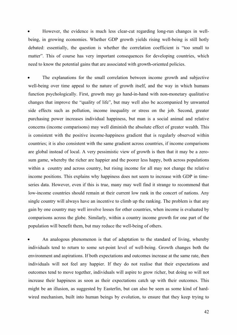
• However, the evidence is much less clear-cut regarding long-run changes in well-
being, in growing economies. Whether GDP growth yields rising well-being is still hotly
debated: essentially, the question is whether the correlation coefficient is “too small to
matter”. This of course has very important consequences for developing countries, which
need to know the potential gains that are associated with growth-oriented policies.
• The explanations for the small correlation between income growth and subjective
well-being over time appeal to the nature of growth itself, and the way in which humans
function psychologically. First, growth may go hand-in-hand with non-monetary qualitative
changes that improve the “quality of life”, but may well also be accompanied by unwanted
side effects such as pollution, income inequality or stress on the job. Second, greater
purchasing power increases individual happiness, but man is a social animal and relative
concerns (income comparisons) may well diminish the absolute effect of greater wealth. This
is consistent with the positive income-happiness gradient that is regularly observed within
countries; it is also consistent with the same gradient across countries, if income comparisons
are global instead of local. A very pessimistic view of growth is then that it may be a zero-
sum game, whereby the richer are happier and the poorer less happy, both across populations
within a country and across country, but rising income for all may not change the relative
income positions. This explains why happiness does not seem to increase with GDP in time-
series data. However, even if this is true, many may well find it strange to recommend that
low-income countries should remain at their current low rank in the concert of nations. Any
single country will always have an incentive to climb up the ranking. The problem is that any
gain by one country may well involve losses for other countries, when income is evaluated by
comparisons across the globe. Similarly, within a country income growth for one part of the
population will benefit them, but may reduce the well-being of others.
• An analogous phenomenon is that of adaptation to the standard of living, whereby
individuals tend to return to some set-point level of well-being. Growth changes both the
environment and aspirations. If both expectations and outcomes increase at the same rate, then
individuals will not feel any happier. If they do not realise that their expectations and
outcomes tend to move together, individuals will aspire to grow richer, but doing so will not
increase their happiness as soon as their expectations catch up with their outcomes. This
might be an illusion, as suggested by Easterlin, but can also be seen as some kind of hard-
wired mechanism, built into human beings by evolution, to ensure that they keep trying to
42

improve their lot (Rayo and Becker, 2007).
• One crucial question in this literature is the relative importance of absolute versus
relative income concerns. Is the welfare effect of income entirely relative? And is the
relative/absolute proportion the same in developing and developed countries? Empirical
evidence on the extent of income comparisons is much scarcer in developing countries. The
evidence that we do have so far contains two important lessons: income comparisons do seem
to affect subjective well-being even in very poor countries; however, adaptation may be more
of a rich country phenomenon.
• Finally, growth and development do not just concern quantitative increases in
consumption, production and the accumulation of capital. They also involve the qualitative
transformation of political governance and market development. These qualitative and
quantitative processes likely involve take-offs and thresholds. Regime change is an important
dimension of these non-linear changes. It is striking that such regime changes are visible in
subjective satisfaction measures. The case of Transition countries is particularly impressive in
this respect: average life satisfaction scores closely mirror changes in GDP for about the first
ten years of the transition process, until the regime becomes more stable. By way of contrast,
in given stable regimes, such as France, we no longer find any relationship between GDP
growth and life satisfaction changes. Our interpretation is that once it becomes stable, the
regime becomes the population’s frame of reference.
• While it is not easy to find large welfare benefits of growth using subjective well-
being, there is nonetheless an interesting finding concerning the level and distribution of
subjective well-being depending on the country’s level of development. The stylized facts are
as follows: (i) average SWB rises with GDP per capita, but (ii) the standard deviation of SWB
falls with GDP per capita. As such, (iii) there is a strong negative relationship between the
average and standard deviation of SWB within a country. Consequently, GDP growth reduces
the inequality in subjective well-being. This is certainly a desirable outcome. If individuals
are risk averse, then behind the veil of ignorance they would prefer a society in which well-
being is more equally distributed, ceteris paribus.
• The recourse to subjective measures of well-being is particularly welcome for
assessing social phenomena that are not measurable using the standard approach of revealed
preference. Whenever social interactions, social preferences or externalities are involved, it
43
becomes more difficult to trace out the link from individual preferences to individual actions.
There is no price one can pay to buy less inflation, unemployment or income inequality.
• However, subjective variables should be used as a complement to action-revealed
preferences, rather than as a replacement. When people clearly vote with their feet, it is
difficult to dismiss their actions on the ground that the message is not confirmed in subjective
data. With respect to growth and well-being, as long as international migrations remain
clearly unidirectional, from low- to high-income countries, it would appear extremely difficult
to argue that GDP growth, in the mind of less-developed countries, does not bring higher
well-being. The revealed preferences here are consistent with the cross-sectional evidence of a
positive income-well-being gradient.
• Our stand is that the dynamic evidence based on subjective well-being is much less
solid than the cross-sectional and panel evidence, based on individual data. This is because
cross-country time-series comparisons are based on aggregate measures, which, by definition,
have lower variance and are less powerful in terms of statistical inference. Moreover, it is
possible that the satisfaction judgements expressed on a bounded-scale yield relative
judgements by their very nature, due to the relation between outcomes and the set of
possibilities (represented by the bounded scale). In this case, it is to be expected that only a
small minority of individuals choose the 10th rung on the scale, which is interpreted as
“having it all”. De facto, quantitative variables, such as fertility, life expectancy or literacy,
exhibit much clearer trends over time than do these bounded-scale qualitative variables, such
as governance indicators.
• The relationship between income growth and well-being is still the object of ongoing
debates that would undoubtedly be better illuminated by the development of panel surveys of
the populations of low-income countries.
44

REFERENCES
Akay, A., and Martinsson, P. (2008). "Does Relative Income Matter for the Very Poor? Evidence from Rural Ethiopia". IZA, Discussion Paper No. 3812.
Akay, A., Martinsson, P., and Medhin, H. (2009). "Does Positional Concern Matter in Poor Societies? Evidence from a Survey Experiment in Rural Ethiopia". IZA, Discussion Paper No. 4354.
Alesina, A. and Giuliano, P. (2008). Preferences for Redistribution. Harvard University and UCLA mimeo.
Alpizar, F., Carlsson, F., and Johansson-Stenman, O. (2005). "How much do we care about absolute versus relative income and consumption?". Journal of Economic Behavior and Organization, 56, 405-421.
Andersson, F. (2006). "Is Concern for Relative Consumption a Function of Relative Consumption?". Göteborg University, mimeo.
Appleton, S., and Song, L. (2008). "Life Satisfaction in Urban China: Components and Determinants". World Development, 36, 2325-2340.
Barr, A. and Clark, D. (2010). “Do the Poor Adapt to Low Income, Minimal Education and Ill-Health?”, Journal of African Economies, 19, 257-293.
Becker, G. S., Philipson, T.J. and Soares, R.R. (2005). "The quantity and quality of life and the evolution of world inequality". American Economic Review, 95, 277-291
Blanchflower D.G. (2008). "International evidence on well-being". IZA Discussion Paper No. 3354.
Blanchflower D.G. and Oswald A. (2004). "Well-being over time in Britain and the USA". Journal of Public Economics, 88, 1359-1386
Blanchflower D.G. and Oswald A. (2005). "Happiness and the Human development index: the paradox of Australia". Australian Economic Review, 38, 307-318
Bookwalter, J., and Dalenberg, D. (2010). "Relative to What or Whom? The Importance of Norms and Relative Standing to Well-Being in South Africa". World Development, 38, 345-355.
Brickman, P., D., C., and Janoff-Bulman, R. (1978). "Lottery winners and accident victims: Is happiness relative?". Journal of Personality and Social Psychology, 36, 917-927.
Brockmann, H., Delhey, J., Welzel, C., and Yuan, H. (2009). "The China Puzzle: Falling Happiness in a Rising Economy". Journal of Happiness Studies, 10, 387-405.
Brown, G., Gardner, J., Oswald, A.J., and Qian, J. (2008). "Does Wage Rank Affect Employees' Wellbeing?". Industrial Relations, 47, 355 - 389.
45

Brown, P., Bulte, E. and Zhang, X. (2010). “Positional Spending and Status Seeking in Rural China.” Journal of Development Economics, forthcoming.
Burchardt, T. (2005). "Are One Man's Rags Another Man's Riches? Identifying Adaptive Preferences Using Panel Data". Social Indicators Research, 74, 57-102.
Card, D., Mas, A., Moretti, E. and Saez, E. (2010). “Inequality at Work: The Effect of Peer Salaries on Job Satisfaction”, NBER Working Paper No. 16396.
Carlsson, F., Gupta, G., and Johansson-Stenman, O. (2009). "Keeping up with the Vaishyas Caste and relative standing in India". Oxford Economic Papers, 61, 52-73.
Castilla, C. (2010). “Subjective poverty and reference dependence”. UNU-WIDER Working
Paper No. 2010/76. Clark, A.E. (1996). "L'utilité est-elle relative? Analyse à l'aide de données sur les ménages".
Economie et Prévision, 121, 151-164. Clark, A.E. (1999). "Are Wages Habit-Forming? Evidence from Micro Data". Journal of
Economic Behavior and Organization, 39, 179-200. Clark, A.E. (2001). "What Really Matters in a Job? Hedonic Measurement Using Quit Data".
Labour Economics, 8, 223-242. Clark, A.E. (2003). "Unemployment as a Social Norm: Psychological Evidence from Panel
Data". Journal of Labor Economics, 21, 323-351. Clark, A.E., Frijters, P., and Shields, M. (2008). "Relative Income, Happiness and Utility: An
Explanation for the Easterlin Paradox and Other Puzzles". Journal of Economic Literature, 46, 95-144.
Clark, A.E., Georgellis, Y. and Sanfey, P. (1998). "Job Satisfaction, Wage Changes and
Quits: Evidence from Germany". Research in Labor Economics, 17, 95-121.
Clark, A.E. and Fischer, J.A.V. (2009). in OECD, 2009. Subjective well-being and social policy.
Clark, A.E., Knabe, A., and Rätzel, S. (2010). "Boon or Bane? Others' Unemployment, Well-being and Job Insecurity". Labour Economics, 17, 52-61.
Clark, A.E., Kristensen, N., and Westergård-Nielsen, N. (2009). "Economic Satisfaction and
Income Rank in Small Neighbourhoods". Journal of the European Economic Association, 7, 519-527.
Clark, A.E., and Oswald, A.J. (1996). "Satisfaction and Comparison Income". Journal of
Public Economics, 61, 359-81. Clark, A.E., and Senik, C. (2010). "Who compares to whom? The anatomy of income
comparisons in Europe". Economic Journal, 120, 573-594.
46

Cohen, S., Doyle, W., Turner, R., Alper, C., and Skoner, D. (2003). "Emotional style and
susceptibility to the common cold". Psychosomatic Medicine, 65, 652-657.
Cojocaru, A. (2010). "On relative status inference when reference groups are unobserved: a cautionary tale". University of Maryland, mimeo.
Corazzini L., Esposito L., Majorano F. “Reign in hell or serve in heaven? A cross-country journey into the relative vs absolute perceptions of well being”. University of Padua, mimeo.
Cummins, R. (2003). "Normative life satisfaction: measurement issues and a homeostatic model". Social Indicators Research, 64, 225-256.
Danner, D., Snowdon, D., and Friesen, W. (2001). "Positive Emotions in Early Life and Longevity: Findings from the Nun Study". Journal of Personality and Social Psychology, 80, 804-813.
Davidson, R. (2004). "Well-being and affective style: neural substrates and biobehavioural
correlates". Philosophical Transactions of the Royal Society, B, 359, 1395–1411.
Deaton, A. (2008). "Income, Health and Well-Being around the World: Evidence from the Gallup World Poll". Journal of Economic Perspectives, 22, 53-72.
Di Tella, R., Haisken-De New, J. and MacCulloch, R. (2007). "Happiness Adaptation to Income and to Status". Harvard Business School, mimeo.
Di Tella, R., and MacCulloch, R. (2006). "Some Uses of Happiness Data in Economics". Journal of Economic Perspectives, 20, 25-46.
Di Tella, R., and MacCulloch, R. (2008). "Gross National Happiness as an Answer to the Easterlin Paradox?". Journal of Development Economics, 86, 22-42.
Di Tella, R., and MacCulloch, R. (2010). "Happiness Adaptation to Income Beyond "Basic Needs"". In E. Diener, J. Helliwell, and D. Kahneman (Eds.), International Differences in Well-Being. Oxford: Oxford University Press.
Di Tella, R., MacCulloch, R.J., and Oswald, A.J. (2001). "Preferences over Inflation and Unemployment: Evidence from Surveys of Happiness". American Economic Review, 91, 335-341.
Di Tella, R., MacCulloch, R.J., and Oswald, A.J. (2003). "The Macroeconomics of Happiness". Review of Economics and Statistics, 85, 809-827.
Diener E., Helliwell J. and Kahneman D. eds. (2009). International Differences in Wellbeing, Princeton: Princeton University Press.
Diener, E. and Lucas, R.E. (1999). Personality and subjective well-being. In Kahneman, D., Diener, E. and Schwarz, N. (Eds), Foundations of Hedonic Psychology: Scientific Perspectives on Enjoyment and Suffering, Chapter 11. New York: Russell Sage Foundation.
47
Diener, E., Lucas, R., and Scollon, C. (2006). "Beyond the Hedonic Treadmill". American Psychologist, 61, 305-314.
Easterlin, R. (1974). Does Economic Growth Improve the Human Lot? Nations and Households in Economic Growth. P. A. David and W. B. Melvin. Palo Alto, Stanford University Press: 89-125.
Easterlin, R.A. (1995). "Will Raising the Incomes of All Increase the Happiness of All?". Journal of Economic Behavior and Organization, 27, 35-47.
Easterlin R. (2000). "The worldwide standard of living since 1800". Journal of Economic Perspectives, 14, 7-26
Easterlin, R.A. (2001). "Income and Happiness: Towards a Unified Theory". Economic Journal, 111, 465-484.
Easterlin, R. (2003). "Explaining Happiness". Proceedings of the National Academy of Science, 100, 11176-11183.
Easterlin, R. (2005a). "Diminishing Marginal Utility of Income? Caveat Emptor." Social Indicators Research 70, 243-255.
Easterlin, R. (2005b). "Feeding the Illusion of Growth and Happiness: A Reply to Hagerty and Veenhoven". Social Indicators Research, 74, 429-443.
Easterlin R. and Angelescu L. (2009). "Happiness and growth the world over: time series evidence on the Happiness-income paradox", IZA Discussion Paper No. 4060
Easterlin R. and Angelescu L. (2010). "Modern Economic Growth: Cross Sectional and Time Series Evidence" in Kenneth C. Land, ed., Handbook of Social Indicators and Quality of Life Research, forthcoming, New York and London: Springer.
Easterlin R. and Sawangfa O. (2010). "Happiness and Growth: Does the Cross Section Predict Time Trends? Evidence from Developing Countries", in E. Diener, J. Helliwell, and D. Kahneman, eds. International Differences in Well-Being. Princeton, NJ., Princeton University Press, chapter 7, pp. 162-212
Easterlin R. and Zimmermann A. (2006). "Life satisfaction and economic outcomes in Germany in pre and post unification". IZA Discussion Paper No. 2494
Easterlin R. and Zimmermann A. (2009). “Lost in Transition: Life Satisfaction on the Road to Capitalism,” Journal of Economic Behavior and Organization, 71, 130-145.
Fafchamps, M. and Shilpi, F. (2008). “Subjective welfare, isolation, and relative consumption,” Journal of Development Economics, 86, 43-60.
Ferrer-i-Carbonell, A. (2005). "Income and well-being: an empirical analysis of the comparison income effect". Journal of Public Economics, 89, 997-1019.
Ferrer-i-Carbonell, A., and Frijters, P. (2004). "How important is methodology for the estimates of the determinants of happiness?". Economic Journal, 114, 641-659.
48

Fließbach, K., Weber, B., Trautner, P., Dohmen, T., Sunde, U., Elger, C., and Falk, A. (2007). "Social comparison affects reward-related brain activity in the human ventral striatum". Science, 318, 1305-1308.
Freeman, R. (1978). Job satisfaction as an economic variable. American Economic Review, vol. 68, pp. 135-141.
Frey, B.S., and Stutzer, A. (2000). "Happiness, Economy and Institutions". Economic Journal, 110, 918-938.
Frey, B., and Stutzer, A. (2007). "Should National Happiness be Maximized?". University of Zurich, mimeo.
Fujita, F., and Diener, E. (2005). "Life Satisfaction Set Point: Stability and Change". Journal of Personality and Social Psychology, 88, 158-164.
Gao, W., and Smyth, R. (2010). "Job satisfaction and relative income in economic transition: status or signal? The case of urban China". China Economic Review, 21, 442-455.
Gardner, J., and Oswald, A.J. (2006). "Do Divorcing Couples Become Happier by Breaking Up?". Journal of the Royal Statistical Society, 169, 319-336.
Graham, C. and Felton, A. (2006). "Inequality and happiness: Insights from Latin America". Journal of Economic Inequality, 4, 107-122.
Goedhart, T., Halberstadt, V., Kapteyn, A. and Van Praag, B.M. (1977). “The poverty line: Concept and measurement”. Journal of Human Resources, 12, 503-520.
Guillen-Royo, M. (2010), “Reference group consumption and the subjective wellbeing of the poor in Peru”, Journal of Economic Psychology, forthcoming.
Guriev, S., and Zhuravskaya, E. (2009). "(Un)Happiness in Transition". Journal of Economic Perspectives, 23, 143-168.
Guven, C., Senik, C., and Stichnoth, H. (2010). "You can't be happier than your wife. Happiness Gaps and Divorce". IZA, Discussion Paper No. 4599.
Hagerty, M.R., and Veenhoven, R. (2000). "Wealth and Happiness Revisited - Growing Wealth of nations does go with greater happiness". University of California-Davis, mimeo.
Helliwell, J.F. (2003). "How's Life? Combining Individual and National Variables to Explain Subjective Well-Being". Economic Modelling, 20, 331-360.
Herrera, J., Razafindrakoto, M. and Roubaud, F. (2006). “The determinants of subjective poverty: A comparative analysis in Madagascar and Peru”, DIAL Working Paper 2006-01.
Hung-Lin T. and Chiu S.. “Income growth or equal income distribution? Implications of the relative income effect on happiness”. Department of economics Soochow university of Taiwan Working Paper
49

Inglehart, R., Foa, R., Peterson, C., and Welzel, C. (2008). "Development, Freedom, and Rising Happiness: A Global Perspective (1981–2007)". Perspectives on Psychological Science, 3, 264-285.
Inglehart, R., and Rabier, J.R. (1986). "Aspirations Adapt to Situations - But Why Are the Belgians so Much Happier than the French? A Cross-Cultural Analysis of the Subjective Quality of Life". In F.M. Andrews (Ed.), Research on the Quality of Life. Ann Arbor: Institute for Social Research University of Michigan.
Inter-American Development Bank (2008). Beyond Facts: Understanding Quality of Life. Cambridge, Mass.: Harvard University Press.
Johannsson-Stenman, O., Carlsson, F., and Daruvala, D. (2002). "Measuring Future Grandparents' Preferences for Equality and Relative Standing". Economic Journal, 112, 362-383.
Kahneman D. and Deaton A., 2010. “High income improves evaluation of life but not emotional well-being”, PNAS, Princeton Center for Health and Well-Being
Kahneman, D., and Tversky, A. (1979). "Prospect Theory: An Analysis of Decision Under Risk". Econometrica, 47, 263-291.
Kenny C. (2005). "Does development make you happy? Subjective well-being and economic growth in developing countries". Social Indicators Research, 73, 199-219
Kingdon, G., and Knight, J. (2007). "Community, Comparisons and Subjective Well-being in a Divided Society". Journal of Economic Behavior and Organization, 64, 69-90.
Knight J. and Gunatilaka R., (2009). "Income, Aspirations and the Hedonic Treadmill in a Poor Society," University of Oxford Discussion Paper N°468.
Knight, J., and Gunatilaka, R. (2010a). "Great Expectations? The Subjective Well-being of Rural–Urban Migrants in China". World Development, 38, 113-124.
Knight, J., and Gunatilaka, R. (2010b). "The rural-urban divide in China: Income but not happiness?" Journal of Development Studies, 46, 506-29.
Knight J., Song L. and Gunatilaka R. (2007). “Subjective well-being and its determinants in rural China”. China Economic Review, 20, 635-649.
Kristensen, N. and Westergaard-Nielsen, N. (2006). "Job satisfaction and quits - Which job characteristics matters most?" Danish Economic Journal, 144, 230-248.
Kuegler, A. (2009). "A Curse of Comparison? Evidence on Reference Groups for Relative Income Concerns". World Bank, Policy Research Working Paper Series No. 4820.
Layard, R. (2003). "Happiness: Has Social Science A Clue?". LSE, mimeo.
Layard, R. (2005). Happiness: Lessons from a New Science. London: Penguin.
50

Layard R., Mayraz G. and Nickell S. (2008). “The Marginal Utility of Income”, Journal of Public Economics, 92, 1846-1857.
Layard R., Mayraz G. and Nickell S., (2010). “Does Relative Income Matter? Are the Critics Right?” in E. Diener, J. F. Helliwell, and D. Kahneman (ed.), International Differences in Well-Being, Oxford University Press.
Luttmer, E. (2005). "Neighbors as Negatives: Relative Earnings and Well-Being". Quarterly Journal of Economics, 120, 963-1002.
McBride, M. (2001). "Relative-income Effects on Subjective Well-being in the Cross-section". Journal of Economic Behavior and Organization, 45, 251-278.
Mishra, V., Nielsen, I. and Smyth, R. (2010). “Relative Income, Temporary Life Shocks and Subjective Wellbeing in the Long-run”, Monash University, mimeo.
Oswald, A.J. (1997). "Happiness and economic performance". Economic Journal, 107, 1815-31.
Palmore, E. (1969). "Predicting Longevity: A Follow-Up Controlling for Age". Gerontologist, 9, 247-50.
Pischke, S. (2010). "Money and Happiness: Evidence from the Industry Wage Structure". LSE, mimeo.
Polity IV Project: Political Regime Characteristics and Transitions, 1800-2009. Monty G. Marshall, Director Monty G. Marshall and Keith Jaggers, Principal Investigators, Center for Systemic Peace and Colorado State University; Ted Robert Gurr, Founder, University of Maryland, http://www.systemicpeace.org/polity/polity4.htm.
Pradhan, M. and Ravallion, M. (1998). “Measuring poverty using qualitative perceptions of welfare”. World Bank and the University of Amsterdam Working paper
Pritchett, L. and Summers, L. (1996). "Wealthier is Healthier." Journal of Human Resources, 31, 841-868.
Ravallion M. and Lokshin M. (2010). “Who cares about relative deprivation?” Journal of Economic Behavior & Organization, 73, 171-185.
Rayo, L., and Becker, G.S. (2007). "Evolutionary Efficiency and Happiness". Journal of Political Economy, 115, 302-37.
Rojas, M. (2010). “Relative Income and Well-Being in Latin America”, Universidad Popular Autónoma del Estado de Puebla, mimeo.
Rojas, M. and Jiménez, E. (2007). “Pobreza Subjetive en México: El Papel de las Normas de Evaluación de Ingreso”, Universidad Popular Autónoma del Estado de Puebla, mimeo.
Sandvik, E., Diener, E. and Seidlitz, L. (1993). Subjective well-being: the convergence and stability of self and non self report measures. Journal of Personality, vol. 61, pp. 317-342.
51
Sen, A. (2001). Development as Freedom. New York: Alfred Knopf.
Senik, C. (2004). "When Information Dominates Comparison: A Panel Data Analysis Using Russian Subjective Data". Journal of Public Economics, 88, 2099-2123.
Senik, C. (2005). "Income Distribution and Well-Being: What Can we Learn from Subjective Data?". Journal of Economic Surveys, 19, 43-63.
Senik, C. (2008). "Ambition and jealousy. Income interactions in the "Old" Europe versus the "New" Europe and the United States". Economica, 75, 495-513.
Senik C. (2009). “Income Distribution and Subjective Happiness: A Survey”, OECD Social Employment and Migration Working Papers n° 96. Published as Income distribution and subjective well-being, in OECD, 2009, Subjective well-being and social policy.
Smyth, R. and Qian, X. (2008). "Inequality and Happiness in Urban China." Economics Bulletin, 4, 1-10.
Solnick, S., and Hemenway, D. (2005). "Are Positional Concerns Stronger in Some Domains than in Others?". American Economic Review, 95, 147-151.
Stark, O., and Taylor, J.E. (1991). "Migration Incentives, Migration Types: The Role of Relative Deprivation". Economic Journal, 101, 1163-1178.
Stevenson, B., and Wolfers, J. (2008), “Economic Growth and Subjective Well-Being: Reassessing the Easterlin Paradox”, Brookings Papers on Economic Activity, Spring.
Stutzer, A. (2004), “The Role of Income Aspirations in Individual Happiness” Journal of Economic Behaviour and Organization 54, 1, 89-109.
Takahashi, H., Kato, M., Matsuura, M., Mobbs, D., Suhara, T., and Okubo, Y. (2009). "When your gain is my pain and your pain is my gain: Neural correlates of envy and Schadenfreude". Science, 323, 937-939.
Urry, H.L., Nitschke, J. B., Dolski, I., Jackson, D. C., Dalton, K. M., Mueller, C. J., Rosenkranz, M.A., Ryff, C. D., Singer, B.H. and Davidson, R.J. (2004). Making a life worth living: Neural correlates of well-being. Psychological Science, vol. 15, pp. 367-372.
Van de Stadt, H., Kapteyn, A., and Van de Geer, S. (1985). "The Relativity of Utility: Evidence from Panel Data". Review of Economics and Statistics, 67, 179-187.
Van Praag, B.M. (1971). "The Welfare Function of Income in Belgium: An Empirical Investigation". European Economic Review, 2, 337-369.
Van Praag, B.M. (1991). "Ordinal and Cardinal Utility". Journal of Econometrics, 50, 69-89.
Van Praag, B. and Frijters, P. (1999), The measurement of welfare and well-being: the Leyden approach” in D. Kahneman, E. Diener and N. Schwarz Wellbeing; The Foundations of Hedonic Psychology, New York: Russell Sage Foundation.
52

Vendrik, M., and Woltjer, G. (2006). "Happiness and Loss Aversion: When Social Participation Dominates Comparison". IZA, Discussion Paper No. 2218.
Wolfers, J. (2003). "Is Business Cycle Volatility Costly? Evidence from Surveys of Subjective Well-being". International Finance, 6, 1-26.
Wolfhard K., 2010. "Conspicuous Consumption and Race: Evidence from South Africa," Papers on Economics and Evolution 2010-03, Max Planck Institute of Economics, Evolutionary Economics Group.
Zizzo, D.J., and Oswald, A.J. (2001). "Are People Willing to Pay to Reduce Others' Incomes?". Annales d'Economie et de Statistique, 63-64, 39-65.
53

54
TABLES

Figure 1.A. Income and happiness in the American General Social Survey (1972-2006). Taken from Stevenson and Wolfers (2008).
Figure 1.B. Income and Happiness in a Chinese cross-section.
Source : WVS. China 2007.
We group together the three deciles (7, 8, 9) which were only rarely reported in the Chinese sample. We have dropped the two extreme deciles.
55

Figure 2.A GDP per capita and SWB in the world. Taken from Inglehart, Foa, Peterson, Welzel (2008), p. 269.
56

Figure 2.B. GDP per capita and Life satisfaction. Taken from Deaton (2008), p. 57.
Figure 2.C. GDP per capita and Life satisfaction
Taken from Deaton (2008), p. 57.
57
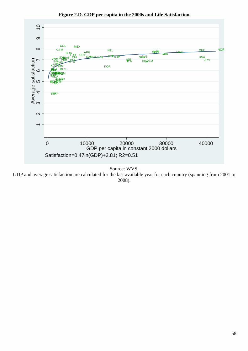
Figure 2.D. GDP per capita in the 2000s and Life Satisfaction
9
58
ETH
UGABFA
TZA
MLI
RWA
KGZGHABGDZMB
MDA
PAK
ZWE
VNM
IND
PHLIDN
UKR
GEOALB
BIH
MARMAC
GTM
EGY
CHN
DZA
IRN
ROM
BGR
JORTHA
RUS
COL
PERZAFBRA
MYS
TURPOL
CHL
MEX
URYARG
SAUTTO SVN
KOR
NZL
CYPESPISRITA
SGPAUSFRADEU
CANNLDFINGBR SWE
USA
CHE
JPN
NOR87
65
43
10A
vera
ge s
atis
fact
ion
21
0 10000 20000 30000 40000GDP per capita in constant 2000 dollars
Satisfaction=0.47ln(GDP)+2.81; R2=0.51
Source: WVS.
GDP and average satisfaction are calculated for the last available year for each country (spanning from 2001 to 2008).

Figure 3.A The American paradox. Happiness and Real GDP per Capita, United States, 1972-2002 Taken from Easterlin and Angelescu (2007).
Figure 3.B Misleading cross-sections. Actual versus predicted happiness in Japan. 1958-1987. Taken from Easterlin (2005).
59

Figures 4.A to 4.E are taken from Inglehart et al. (2008, statistical appendix).
Figure 4.A. The Happiness Trend in India
2
2.2
2.4
2.6
2.8
3
3.2
1970 1975 1980 1985 1990 1995 2000 2005 2010
mean happiness in India, 1975-2006(1= not at all happy, 4=very happy)
Figure 4.B. The Happiness Trend in
Mexico
2
2.2
2.4
2.6
2.8
3
3.2
3.4
3.6
1970 1975 1980 1985 1990 1995 2000 2005 2010
mean happiness in Mexico, 1975-2006(1= not at all happy, 4=very happy)
Figure 4.C. The Happiness Trend in
Puerto Rico
2
2.2
2.4
2.6
2.8
3
3.2
3.4
3.6
1960 1965 1970 1975 1980 1985 1990 1995 2000 2005 2010
mean happiness in Puerto Rico, 1963-2000(1= not at all happy, 4=very happy)
Figure 4.D. The Happiness Trend in
South Africa
2
2.2
2.4
2.6
2.8
3
3.2
3.4
1970 1975 1980 1985 1990 1995 2000 2005 2010
mean happiness in South Africa, 1981-2006(1= not at all happy, 4=very happy)
Figure 4.E. The Happiness Trend in China
2
2.2
2.4
2.6
2.8
3
3.2
3.4
3.6
1985 1990 1995 2000 2005 2010
mean happiness in China, 1990 - 2006(1= not at all happy, 4=very happy)
60
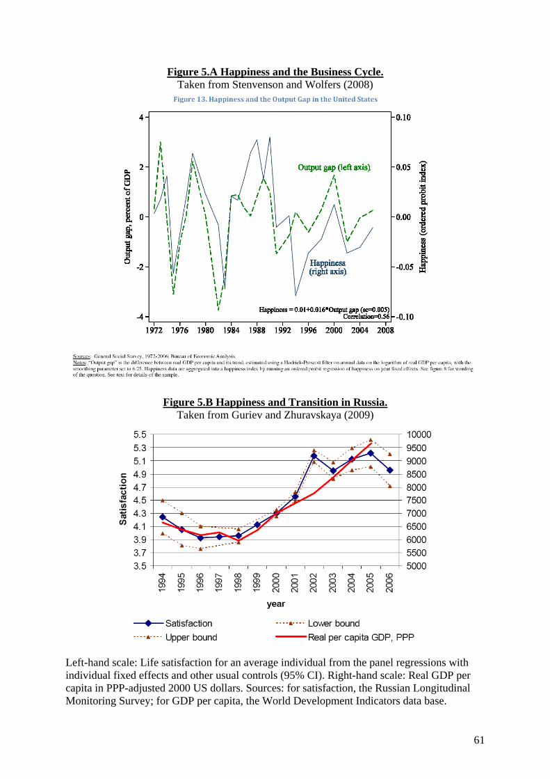
Figure 5.A Happiness and the Business Cycle. Taken from Stenvenson and Wolfers (2008)
Figure 5.B Happiness and Transition in Russia. Taken from Guriev and Zhuravskaya (2009)
Left-hand scale: Life satisfaction for an average individual from the panel regressions with individual fixed effects and other usual controls (95% CI). Right-hand scale: Real GDP per capita in PPP-adjusted 2000 US dollars. Sources: for satisfaction, the Russian Longitudinal Monitoring Survey; for GDP per capita, the World Development Indicators data base.
61

Figure 5.C Happiness and Transition in several countries. Taken from Easterlin and Zimmerman (2009)
62

Figure 6. GDP, and the Average and Standard Deviation of Happiness
NZL_2004
ITAF
CAN_2006NLD_2006FIN_2005
GBR_2006SWE_2006
A_2006
CHE_2007NOR_2008
CYP_2006ESP_2007
_2005
AUS_2005
RA_2006
US
ETH_2007
UGA_2001BFA_2007
TZA_2001
MLI_2007
RWA_2007
KGZ_2003
GHA_2007
BGD_2002
ZMB_2007
MDA_2006
PAK_2001
ZWE_2001
VNM_2006
IND_2006
PHL_2001
IDN_2006
UKR_2006_2001
GEO_2008ALB_2002
BIH_2001
MAR_2007MAC_2001
GTM_2005
EGY_2008
CHN_2007
DZA_2002
IRN_2007
ROM_2005
BGR_2006
JOR_2007THA_2007
RUS_2006
COL_2005
PER_2008ZAF_2007
BRA_2006
MYS_2006
TUR_2007
POL_2005CHL_2005
MEX_2005
URY_2006ARG_2006
SAU_2003TTO_2006SVN_2005
KOR_2005
ISR_2001SGP_2002
DEU_2006JPN_2005
45
67
89
Ave
rage
sat
isfa
ctio
n
4 6 8 10 12Log GPD per capita in cst 2000 dol
R2=.51
Average satisfaction and ln(GDP)
FRA_
ITA_2005
AND_2005
5
ESP_2007
06
GBR_2006SWE_2006
NLD_2006
CAN_2006FIN_2005
ZL_2004
CHE_2007
NOR_2008
2006
USA_2006AUS_200
CYP_20
N
TZA_2001
ZWE_2001
IRQ_2006
PAK_2001
GEO_2008
RWA_2007ETH_2007
MAC_2001
ALB_2002BGR_2006
MAR_2007
MDA_2006BFA_2007
_2001UGA_2001
DZA_2002
ROM_2005BIH_2001
BGD_2002
EGY_2008
IND_2006UKR_2006
SRB_2006
ZMB_2007MLI_2007GHA_2007
RUS_2006
KOR_2005HKG_2005
IRN_2007
KGZ_2003PHL_2001
_2006
CHN_2007
MYS_2006
IDN_2006
DEU_2006
JPN_2005
POL_2005
PER_2008ISR_2001
VNM_2006
ZAF_2007
JOR_2007
THA_2007SGP_2002
SVN_2005CHL_2005
TTO_2006SAU_2003TUR_2007
URY_2006
BRA_2006
ARG_2006
GTM_2005MEX_2005
COL_2005_2001
1.5
22.
53
3.5
S.D
. of s
atis
fact
ion
4 5 6 7 8 9Average satisfaction
R2=.32
Life satisfaction: Av. and S.D.
NZL_2004
CYP_2006
ESP_2007
ITA_2005
A_2006
CAN_2006
NLD_2006
FIN_2005GBR_2006SWE_2006CHE_2007
NOR_2008
AUS_2005
FR
USA_2006
ETH_2007
UGA_2001
BFA_2007
TZA_2001
MLI_2007
RWA_2007
KGZ_2003GHA_2007
BGD_2002
ZMB_2007
MDA_2006
PAK_2001
ZWE_2001
VNM_2006
IND_2006
PHL_2001
IDN_2006
UKR_2006
_2001
GEO_2008ALB_2002
BIH_2001
MAR_2007
MAC_2001
GTM_2005
EGY_2008
CHN_2007
DZA_2002
IRN_2007ROM_2005BGR_2006
JOR_2007
THA_2007
RUS_2006
COL_2005
PER_2008
ZAF_2007
BRA_2006
MYS_2006
TUR_2007
POL_2005CHL_2005MEX_2005
URY_2006ARG_2006
SAU_2003TTO_2006
SVN_2005KOR_2005
ISR_2001
SGP_2002
DEU_2006
JPN_2005
1.5
22.
53
3.5
S.D
. of s
atis
fact
ion
4 6 8 10 12Log GPD per capita in cst 2000 dol
R2=.41
S.D. of satisfaction and ln(GDP)
Source: World Values Survey, 1981-2007.
63
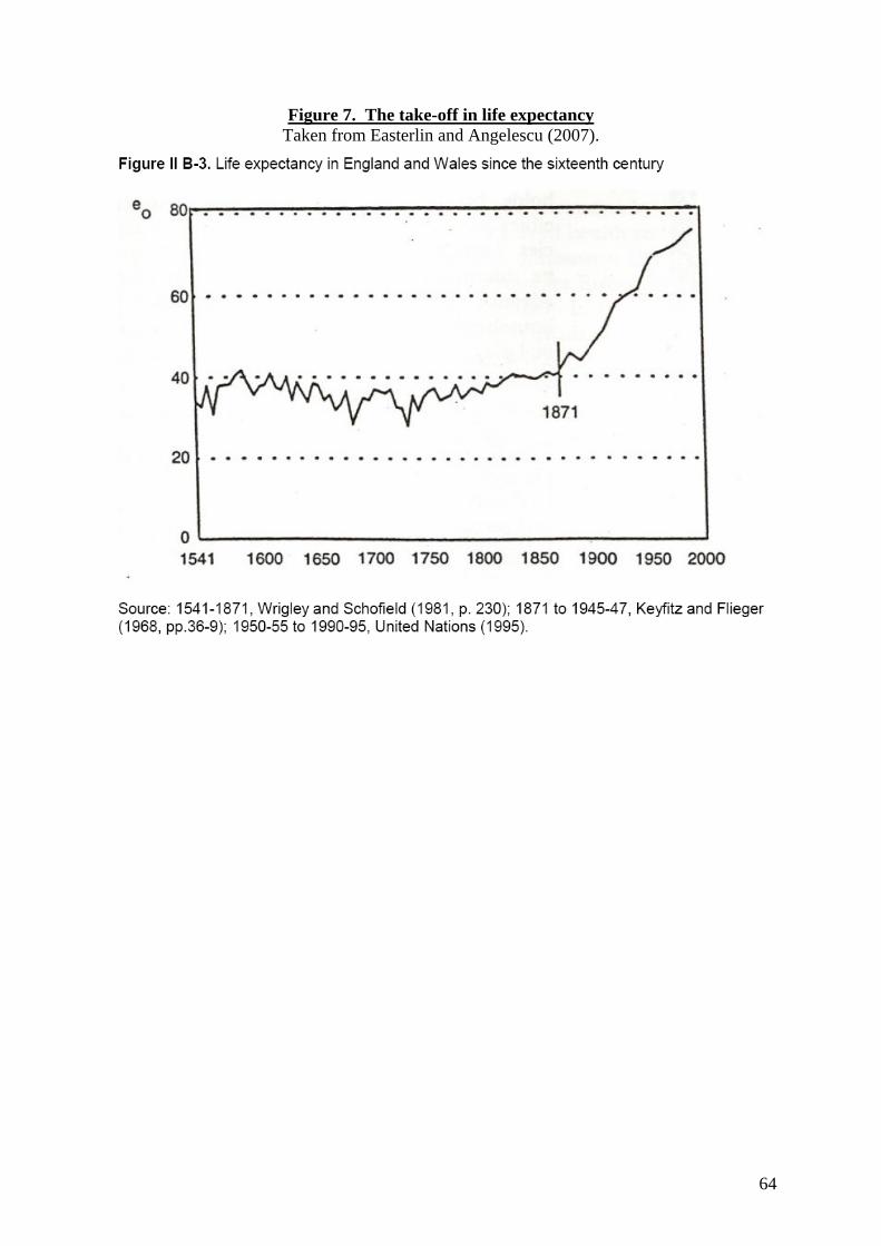
Figure 7. The take-off in life expectancy Taken from Easterlin and Angelescu (2007).
64

Figure 8. GDP Growth, Inequality and Happiness.
Taken from Layard, Mayraz and Nickell (2010, p. 142)
65

Figure 9. The Evolution of Cardinal versus Ordinal Quality of Life Indices over a Period of Growth
1) Asia:
Source: WVS (1981-2008)
66

2) Western countries:
67

Source: WVS (1981-2008)
68

69
APPENDIX
Table A1. Descriptive statistics of the variables from the WVS database
Variable No.
CountriesNo.
Years Mean value Std.Dev. Min. Max. Source First year
Last year
Average happiness 105 368 3.02 0.27 2.06 3.58 WVS 1981 2008 Average satisfaction 98 251 6.70 1.07 3.73 8.49 WVS 1981 2008 No. of children per woman 96 342 2.12 1.02 1.08 6.79 WDI 1981 2008 Democracy (Freedom House/Imputed Polity) 96 337 8.24 2.34 0.00 10.00 Freedom house 1981 2008 Political Rights 96 337 2.15 1.65 1.00 7.00 Freedom house 1981 2008 GDP growth per year 97 348 3.12 4.82 -14.57 46.50 WDI 1981 2008 GDP per capita in constant 2000 dol 97 348 11536.26 11138.87 175.01 43420.52 WDI 1981 2008 Growth GDP per capita 97 348 2.32 4.64 -14.57 42.86 WDI 1981 2008 GDP per capita in ppp 96 347 16508.83 11547.53 236.94 57034.16 WDI 1981 2008 Gross enrolment rate 95 331 78.87 12.90 32.77 100.00 HDI 1981 2007 Gini index 49 91 39.82 11.80 19.40 60.24 WDI 1989 2007 Life expectancy at birth 96 344 72.89 6.80 42.19 82.51 WDI 1981 2008 Infant mortality rate per 1000 74 254 14.23 19.52 2.50 120.00 WDI 1981 2008 Average trust 98 251 0.30 0.15 0.03 0.74 WVS 1981 2008

Variable description
All variables are available in the World Data Bank: http://www.worldvaluessurvey.org/
Happiness: “If you were to consider your life in general these days, how happy or unhappy would you say you are, on the whole?” (the question and different response categories are the same in the three studies): 1. Not at all happy; 2. Not very happy; 3. Fairly happy; and 4. Very happy.
Life satisfaction: “All things considered, how satisfied are you with your life as a whole these days?”. The response categories go from 1(dissatisfied) to 10 (very satisfied).
Trust: “Generally speaking, would yon say that most people can be trusted or that you cant be too careful in dealing with people?”, Answers: 1. most people can be trusted; 0 . Can't be too careful.
Fertility rate: This measure represents the number of children that would be born to a woman were she to live to the end of her childbearing years and bear children in accordance with the current age-specific fertility rates.
GDP growth: Annual percentage growth rate of GDP at market prices in constant local currency. Aggregate figures are based on constant 2000 U.S. dollars.
GDP per capita in 2000 dollars: GDP per capita is gross domestic product divided by midyear population. Data are in constant U.S. dollars.
Gini index: the Gini index measures the extent to which the distribution of income (or, in some cases, consumption expenditure) among individuals or households within an economy deviates from a perfectly equal distribution. A Lorenz curve plots the cumulative percentages of total income received against the cumulative number of recipients, starting with the poorest individual or household. The Gini index measures the area between the Lorenz curve and a hypothetical line of absolute equality, expressed as a percentage of the maximum area under the line. Thus a Gini index of 0 represents perfect equality, while an index of 100 implies perfect inequality.
Life expectancy at birth: Life expectancy at birth indicates the number of years a newborn infant would live were prevailing patterns of mortality at the time of its birth to stay the same throughout their life.
Infant mortality rate (per 1000 under one): the number of infants dying before reaching age one, per 1,000 live births in a given year.
Gross Enrolment Rate in %: enrolment in primary, second and tertiary education.
Adult Literacy rate in %.
Freedom house (http://www.freedomhouse.org): Political rights that enable people to participate freely in the political process, including the right to vote freely for distinct alternatives in legitimate elections, compete for public office, join political parties and organizations, and elect representatives who have a decisive impact on public policies and are
70

71
accountable to the electorate. The specific list of rights considered varies over the years. Countries are graded between 1 (most free) and 7 (least free).
Democracy: Average of Freedom House and Polity, transformed to a scale 0-10, where 0 is least democratic and 10 most democratic (http://www.govindicators.org ).

A.2 THE INCOME – HAPPINESS NEXUS: SOURCES AND ESTIMATES, SUMMARY.
SUBJECTIVE WELL-BEING MEASURES
- Happiness: If you were to consider your life in general these days, how happy or unhappy would you say you are, on the whole: Not at all happy; not very happy; Fairly happy; Very happy.
- Life satisfaction: All things considered, how satisfied are you with your life as a whole these days? 1 (dissatisfied) – 10 (very satisfied).
1) THE STATIC RELATIONSHIP BETWEEN INDIVIDUAL INCOME AND INDIVIDUAL HAPPINESS
Consensus: higher income higher happiness. In a country, richer individuals are happier than poorer individuals.
Nationally representative household surveys. Individual level analysis. Within-country cross-section estimates.
Western developed countries
German Socio-Economic Panel (GSOEP), British Household Panel Survey (BHPS), Swiss household panel, Australian household survey (HILDA), General Social Survey (America), Japanese household survey, data from Netherlands, Denmark, etc.
European Values Survey (EVS), European Social Survey (ESS), Eurobarometer.
Transition countries
Albania, Bulgaria, Latvia, Romania Russia, Estonia, Lithuania, Hungary, Belarus, Poland, Ukraine, etc.
Life in Transition Survey (LITS, 2006), European Social Survey, European Values Survey.
Asian household surveys
China, India, Shanghai.
African and Middle-East national household surveys
Argentina, Brazil, Chile, Ethiopia, Mexico, Mexico, Nigeria, Peru, South Korea, South Africa (SALDRU), Tanzania, Turkey, Venezuela.
International surveys
World Values Survey (WVS, 1981- 2008, 5 waves, 105 countries).
International Social Survey Program (ISSP, 101 countries)
72

Gallup World Poll (2006, 105 countries).
Latinobarometer (18 countries)
European Social Survey (25 countries)
European Values Survey
2) THE DYNAMIC RELATIONSHIP BETWEEN INDIVIDUAL INCOME AND INDIVIDUAL HAPPINESS
Within country estimates. Individual level panel data analysis.
Consensus: higher income higher happiness. Individuals become happier as they grow richer.
Individual Panel Data in Developed Countries
GSOEP, BHPS, HILDA, data from Netherlands and Denmark.
Individual Panel data in LDCs
RLMS (Russia), ULMS (Ukraine), Peru, LSMS (Tadjikistan).
3) THE STATIC RELATIONSHIP BETWEEN NATIONAL INCOME AND AVERAGE HAPPINESS
Aggregate measures, cross-country estimates.
Consensus: higher income higher happiness. Individuals living in richer countries are happier than those living in poorer countries.
4) THE DYNAMIC RELATIONSHIP BETWEEN NATIONAL INCOME AND AVERAGE HAPPINESS
Aggregate measures, cross-country estimates.
No consensus. Divergent findings.
Income growth does not increase happiness over time
o Easterlin (2005a), Easterlin and Sawangfa (2005, 2009), Easterlin and Angelescu (2007), Easterlin (2009)
o Layard; Brockmann, Delhey, Welzel, Yuan (2009)
Income growth does increase happiness over time
o Stevenson and Wolfers (2008) o Deaton (2008) Gallup (2006) o Helliwell (2002) o Blanchflower (2008)
73

Income growth does increase happiness over time but not always and weakly
o Hagerty and Veenhoven (2000, 2003, 2006), WVS (positive and statistically significant coefficient, but not in all countries).
o Inglehart, Peterson and Welzel (2008): WVS, BHPS, GSS (positive and statistically significant coefficient, but not in all countries), Kenny (2005), idem.
o Layard, Mayraz and Nickell (2010) (positive coefficient but not always statistically significant).
o Oswald (1997) in GSS and Eurobarometer survey series, positive coefficient but not always statistically significant.
o Di Tella and MacCulloch (2008): positive coefficient but low statistical significance.
74


![in press Emotion] Does a culture of happiness increase ... a culture of happiness increase rumination over failure? Lucy McGuirk1, Peter Kuppens2, Rosemary Kingston1, & Brock Bastian3,](https://img.dokumen.tips/doc/110x75/5ac16e907f8b9a5a4e8d214f/in-press-emotion-does-a-culture-of-happiness-increase-a-culture-of-happiness.jpg)


![Creative Lifehacks to Increase Productivity, Health & Happiness [Updated for True U 2014]](https://img.dokumen.tips/doc/110x75/55a201391a28ab33268b45c3/creative-lifehacks-to-increase-productivity-health-happiness-updated-for-true-u-2014.jpg)


