MNRAS 000, 1–27 (2017) Preprint 27 April 2017 Compiled using MNRAS LATEX style file v3.0

Wide Binaries in Tycho-Gaia: Search Method and theDistribution of Orbital Separations

Jeff J. Andrews1,2?, Julio Chaname3,4, Marcel A. Agueros51 Foundation for Research and Technology - Hellas, IESL, Voutes, 71110 Heraklion, Greece2 Physics Department & Institute of Theoretical & Computational Physics, University of Crete, 71003 Heraklion, Crete, Greece3 Instituto de Astrofısica, Pontificia Universidad Catolica de Chile, Av. Vicuna Mackenna 4860, 782-0436 Macul, Santiago, Chile4 Millennium Institute of Astrophysics, Santiago, Chile5 Department of Astronomy, Columbia University, 550 West 120th Street, New York, NY 10027, USA

Accepted XXX. Received YYY; in original form ZZZ

ABSTRACTWe mine the Tycho-Gaia astrometric solution (TGAS) catalog for wide stellar bina-ries by matching positions, proper motions, and astrometric parallaxes. We separategenuine binaries from unassociated stellar pairs through a Bayesian formulation thatincludes correlated uncertainties in the proper motions and parallaxes. Rather thanrelying on assumptions about the structure of the Galaxy, we calculate Bayesian priorsand likelihoods based on the nature of Keplerian orbits and the TGAS catalog itself.We calibrate our method using radial velocity measurements and obtain 6196 high-confidence candidate wide binaries with projected separations s . 1 pc. The normaliza-tion of this distribution suggests that at least 0.6% of TGAS stars have an associated,distant TGAS companion in a wide binary. We demonstrate that Gaia’s astrometryis precise enough that it can detect projected orbital velocities in wide binaries withorbital periods as large as 106 yr. For pairs with s <∼ 4 × 104 AU, characterization

of random alignments indicate our contamination to be ≈5%. For s . 5 × 103 AU,our distribution is consistent with Opik’s Law. At larger separations, the distributionis steeper and consistent with a power-law P(s) ∝ s−1.6; there is no evidence in ourdata of any bimodality in this distribution for s . 1 pc. Using radial velocities, wedemonstrate that at large separations, i.e., of order s ∼ 1 pc and beyond, any potentialsample of genuine wide binaries in TGAS cannot be easily distinguished from ionizedformer wide binaries, moving groups, or contamination from randomly aligned stars.

Key words: binaries: visual – astrometry – proper motions – parallaxes

1 INTRODUCTION

Roughly half of all main-sequence stars are found in binarysystems with orbital separations extending from ∼10 R� to∼pc (Duquennoy & Mayor 1991; Fischer & Marcy 1992;Raghavan et al. 2010; Duchene & Kraus 2013). Unresolvedbinaries at the smallest separations are typically found byidentifying radial velocity (RV) variations indicative of or-bital motion, while binaries at intermediate separations canbe identified by observing the stars’ motions through theirorbits over many years (Raghavan et al. 2010), or by identi-fying in decades of archival data dips in a star’s luminositycaused by eclipses due to an unseen stellar companion (Ro-driguez et al. 2016). At the largest separations, stars are typ-ically associated by watching them move through the solarneighborhood in the same direction and at the same rate;

? Contact e-mail: andrews@physics.uoc.gr

these common proper motion pairs have separations from102 to ≥104 AU (Luyten 1971).

The orbits of wide binaries may represent a significantfraction of the size of the clusters within which most stars areborn (Lada & Lada 2003). Such widely separated binariesare likely to form during the dissolution of a single-age stellarcluster (Kouwenhoven et al. 2010; Moeckel & Clarke 2011)or from the evolution of higher-order systems (Reipurth &Mikkola 2012; Elliott & Bayo 2016). Since these pairs maybe dynamically removed or slowly separated from the clus-ter (Theuns 1992; Fujii et al. 2012), the population of widebinaries can probe the physics of cluster dissolution (Kroupaet al. 2001; Kouwenhoven et al. 2010). Additionally, triplesor higher order systems formed via the fragmentation of cir-cumbinary disks (Bonnell & Bate 1994) may evolve dynami-cally into independent binaries (Bate et al. 2002; Moeckel &Bate 2010) or stable, hierarchical triple systems (Reipurth& Mikkola 2012). The observed distribution of orbital peri-

© 2017 The Authors

arX

iv:1

704.

0782

9v1

[as

tro-

ph.S

R]

25

Apr

201

7

2 Andrews, Chaname, & Agueros

ods is therefore the result of the physics of formation and ofsubsequent dynamical reprocessing (Kroupa 1995; Jiang &Tremaine 2010; Moeckel & Clarke 2011).

Beyond ≈103 AU, the components of wide binaries arenot expected to interact significantly over their lifetimes.These pairs can be considered mini-open clusters (Binney &Tremaine 1987; Soderblom 2010) and are uniquely power-ful for answering questions that cannot be addressed withother stellar systems. For example, wide binaries consistingof white dwarfs, subdwarfs, or M-dwarfs with FGK mainsequence companions have been used to calibrate metal-licity scales and age-rotation relations (Lepine et al. 2007;Rojas-Ayala et al. 2010; Garces et al. 2011; Chaname &Ramırez 2012; Li et al. 2014). Other white dwarf-main se-quence pairs and double white dwarfs have been used todetermine the initial-to-final mass relation for white dwarfs(Finley & Koester 1997; Zhao et al. 2012; Andrews et al.2015). At the widest separations, binaries are affected by in-teractions with other stars, giant molecular clouds, and theGalactic tide, each of which acts to disrupt them stochasti-cally (Weinberg et al. 1987; Jiang & Tremaine 2010). Thesebinaries have been used as probes of the gravitational poten-tial of their host, including the contribution of dark objectsand of dark matter in general (Bahcall et al. 1985; Yoo et al.2004; Hernandez & Lee 2008; Quinn et al. 2009; Monroy-Rodrıguez & Allen 2014; Penarrubia et al. 2016).

We define a bona fide wide binary as a system of twostars whose properties are consistent with being gravitation-ally bound to each other. We do not claim that the compo-nents of wide binaries presented in this work are demonstra-bly orbiting their common center of mass, as that would atleast require measurement of the accelerations of the compo-nents or of their orbit on the plane of the sky (e.g., Tokovinin& Kiyaeva 2016). Instead, we regard a pair as a genuine bi-nary when, to the limits of the data, their phase-space co-ordinates are consistent with the hypothesis that they aregravitationally bound to each other.

This definition becomes crucial when considering howwide one can go in a search for wide binaries. Within theMilky Way, a pair of stars cannot remain gravitationallybound for long beyond the separation at which they becomesensitive to the Galactic tidal field. This tidal limit (or Ja-cobi radius) is ≈2 pc for ≈M� stars within the solar neighbor-hood (Yoo et al. 2004; Jiang & Tremaine 2010). Pairs widerthan this limit do exist: they may be wide binaries that havebeen ionized, members of moving groups, the tidal remainsof larger structures, etc. However, as we demonstrate laterin this work, they overlap in observational space with a siz-able population of (false) pairs that occur simply by chance.Given the large variety of astronomical problems that canbenefit from the assembly of reliable samples of wide bi-naries, we argue that pairs beyond the Galactic tidal limitshould not be confused with genuine wide binaries, and welimit our search to pairs with projected separations .1 pc.

The exact form of the distribution of bona fide wide bi-nary separations can help to constrain their formation sce-narios. Although some groups find that this distribution isflat in log space out to the largest separations (followingwhat is known as Opik’s Law; e.g., Opik 1924; Poveda et al.2007; Allen & Monroy-Rodrıguez 2014), the current con-sensus favors a distribution that decreases at larger separa-tions (Chaname & Gould 2004; Lepine & Bongiorno 2007;

Tokovinin & Lepine 2012; Halbwachs et al. 2017). As of yet,however, only a few attempts have been made to link di-rectly the observed orbital separation distribution with mod-els: Kouwenhoven et al. (2010) and Moeckel & Clarke (2011)have both compared N-body simulations of cluster dissolu-tion to the observed orbital separation distribution. One rea-son for this scarcity of comparisons between data and simu-lations is that the observed samples are typically small. Iden-tifying large numbers of wide binaries is difficult, and sam-ples often suffer from significant and hard-to-characterizeobservational biases.

Pioneering work identifying wide binaries focused onsmall, specialized catalogs of stars (Luyten 1971; Wasser-man & Weinberg 1991; Garnavich 1991; Gould et al. 1995).More recent efforts have employed methods of varying com-plexity to systematically search larger, astrometric catalogssuch as those produced by the New Luyten Two-Tenths sur-vey (NLTT; Luyten 1979) and the revised NLTT (rNLTT;Gould & Salim 2003; Salim & Gould 2003), e.g., Allen et al.(2000); Chaname & Gould (2004), the Sloan Digital Sky Sur-vey (SDSS; York et al. 2000), e.g., Sesar et al. (2008); Quinn& Smith (2009); Dhital et al. (2010); Longhitano & Binggeli(2010); Andrews et al. (2012); Baxter et al. (2014); Andrewset al. (2015); Dhital et al. (2015), the Lepine-Shara ProperMotion-North catalog (LSPM; Lepine & Shara 2005), e.g.,Lepine & Bongiorno (2007), and Hipparcos (Perryman et al.1997), e.g., Shaya & Olling (2011); Tokovinin & Lepine(2012). These searches typically fall in one of two categories:there are those where stars are matched using only posi-tion (for instance using a two-point correlation function) andthose where proper motion is included as well (to identifycommon proper motion pairs), corresponding to matchingtwo or four dimensions, respectively, of the six-dimensionalphase space.1

Shaya & Olling (2011) performed the first large-scalesearch for binaries that included Hipparcos parallaxes in amatching algorithm. The additional phase-space dimensionadds a powerful constraint for separating genuine binariesfrom randomly aligned stellar pairs. However, because ofits non-linear dependence on distance and non-trivial priorprobabilities, the inclusion of parallax also adds a significantdegree of complexity to the matching algorithm. Neverthe-less, using a Bayesian formalism, these authors identify over1000 binaries, including several high-probability pairs withprojected separations of ∼pc.

The first data release from the Gaia satellite (Gaia Col-laboration et al. 2016a,b; Lindegren et al. 2016) includes2 × 106 Tycho-2 stars (Høg et al. 2000), for which a Tycho-Gaia astrometric solution (TGAS; Michalik et al. 2015) isprovided. The TGAS catalog is nearly complete to V = 11mag, with stars out to V ≈ 12. Each of these stars haspositions (with uncertainties of ≈0.4 mas), proper motions(uncertainties ≈1.3 mas yr−1), and parallaxes (uncertainties

1 Note that several groups have included photometric distanceestimates in their matching algorithm. Although not used withinthe matching algorithm itself, there have also been efforts to in-

clude RVs (e.g., Latham et al. 1984), astrometric parallaxes (e.g.,Lepine & Bongiorno 2007), or both (Halbwachs et al. 2017) as ex-tra phase-space dimensions to confirm the binary nature of widepairs.

MNRAS 000, 1–27 (2017)

Wide Binaries in TGAS 3

≈0.3 mas, although a systematic bias of ≈0.25 mas has beenidentified in Gaia parallaxes; Stassun & Torres 2016).

Oelkers et al. (2016) and Oh et al. (2016) performedsearches for wide binaries and moving groups in the TGAScatalog, including for subsets with separations >1 pc. Theinitial Oelkers et al. (2016) catalog includes 8516 candidatepairs in which both stars are in TGAS. Although these au-thors use a sophisticated Galactic model to determine therandom alignment likelihood for any particular wide binary,they do not calculate a corresponding likelihood that anybinary could be a genuine pair. Furthermore, while theirmethod combines proper motions, parallaxes, and their asso-ciated uncertainties to identify real pairs, it neglects correla-tions between the proper motion and parallax uncertainties,which can be considerable.

Oh et al. (2016) use an improved method to identifyco-moving stars. These authors calculate the likelihood thata particular pair is a genuinely associated binary and that itis a random alignment of unassociated stars. In calculatingthese two likelihoods, these authors assume a model for thestellar components of the Milky Way.

We describe a Bayesian method for identifying wide bi-naries that combines positions, proper motions, astrometricparallaxes and their correlated uncertainties. Similar to Ohet al. (2016), we calculate two likelihoods for each stellarpair. However, our calculations use a data-based approachand are independent of any assumptions about the struc-ture of the Milky Way.2 We separate genuine binaries fromrandomly aligned pairs using a posterior probability thatcombines these two likelihoods with prior probabilities basedon the local stellar density. We further improve on previouswork by verifying and calibrating our algorithm using two in-dependent methods. First, using our algorithm, we identifyand characterize a set of random alignments by matchingthe catalog to a shifted version of itself, which produces asample containing only random alignments. Second, we usethe subset of our pairs with radial velocity (RV) measure-ments to determine the rate of contamination due to ran-domly aligned stars. Our discussion is focused on identifyingpairs within the TGAS catalog, but our method is designedto be adaptable to any stellar catalog with five-dimensionalastrometry and is scalable to the expanded catalogs expectedfrom future Gaia data releases.

In Section 2, we outline the challenges posed by thesize of the TGAS catalog and the quality of Gaia data. Ourstatistical method for combining positions, proper motions,and parallaxes is described in Section 3. Before applying it tothe full TGAS catalog, we describe in Section 4 our effortsto predict the characteristics of the contamination due tofalse binaries. In Section 5, we assemble our candidate TGASpairs, calibrate our method to set a probability threshold foridentifying real binaries, and estimate our contamination byfalse binaries. We present the resulting catalog of wide bina-ries, and use a low-contamination subset to characterize theprojected separation distribution in Section 6. In Section 7,we compare our sample to pre-TGAS catalogs of wide bina-ries, discuss the impact of our assumptions on our search,

2 Furthermore, Oh et al. (2016) select only those pairs with aparallax signal-to-noise (S/N) ratio >8, whereas we search the

entire TGAS catalog.

address the question of whether we can reliably identify pairsat separations >∼1 pc, and provide some guidance to users ofour catalog. We conclude in Section 8 with a few thoughtsabout identifying wide binaries in future Gaia catalogs. Ap-pendix A is a test of our method on the subset of the rNLTTcatalog with Hipparcos parallaxes; we compare the resultingcatalog with a previously identified catalog of rNLTT widebinaries.

2 CHALLENGES

Hipparcos provided the only data comparable to the TGASdata, for ≈105 stars. Since the number of possible pairs of acatalog of size N is the arithmetic mean N(N − 1)/2, identi-fying binaries in Hipparcos data implies the examination of≈5 × 109 individual pairs of stars. While the TGAS catalogis only 20 times larger than the Hipparcos catalog, the totalnumber of pairs it contains is ≈2 × 1012, a factor of 500 in-crease, and the final Gaia catalog will contain ≈5×1017 indi-vidual pairs. Of course, not every stellar pair need be checked(for instance, one can select a maximum angular search ra-dius around each star), but the ≈N2 scaling with catalogsize is likely unavoidable. Clearly the algorithms developedto search previous astrometric catalogs, even those designedto include Hipparcos parallaxes, need to be rethought.

Furthermore, Gaia’s superb astrometric precision cre-ates new challenges for identifying wide binaries. Given thisprecision, the traditional approach of selecting pairs of starswith identical proper motions will miss a large number oftrue binaries: Gaia is sensitive to the differential orbital ve-locities of many wide binaries.

To illustrate, we generate 104 binaries with separationsa randomly drawn from a flat distribution in log space3 andeccentricities e drawn from a thermal distribution:

P(a) ∝ a−1 ; a ∈ [10 R� : 1 pc] (1)

P(e) ∝ e ; e ∈ [0 : 1). (2)

We further adopt random binary orientation angles todetermine the distribution of the projected separations s andof the projected differences in orbital velocities ∆V .

Figure 1 compares the distribution of our binaries inlog s − log∆V space to Gaia’s astrometric limits. The TGASdata can be used to identify pairs of stars with angular sep-arations as small as ≈2′′ and proper motions as small as≈1.3 mas yr−1. We apply these limits to pairs at three rep-resentative distances, 10, 100, and 500 pc, which allow us totranslate the angular units observed by Gaia into physicalunits. In the top panel of Figure 1, we show the correspond-ing areas in log s − log∆V space for which Gaia can measure∆V , the difference between the two velocity components ofa binary due to orbital motion.

By the final Gaia data release, the astrometry will besubstantially more precise: on-ground processing may allowidentification of stellar pairs with separations as small as

3 Although evidence has indicated that the distribution of wide

binary separations follows a power-law with a somewhat steeperindex than −1 (Chaname & Gould 2004; Lepine & Bongiorno

2007), adopting this flat distribution more clearly demonstrates

the region in s − ∆V space populated by binaries.

MNRAS 000, 1–27 (2017)

4 Andrews, Chaname, & Agueros

2 1 0 1 2 3 4 5 6 7

2

1

0

1

2

3

Log

∆V

(km

s−1)

500 pc

100 pc

10 pc

TGAS

2 1 0 1 2 3 4 5 6 7

Log s (AU)

2

1

0

1

2

3

Log

∆V

(km

s−1)

500 pc

100 pc

10 pc

Future Gaia

Figure 1. The kernel density estimate representation of 104 ran-

domly produced binaries in log s− log∆V space. Binaries with thelargest separations (≈1 pc) should have nearly identical proper

motions. For smaller projected separations, the tangential veloci-

ties may differ by as much as tens of km s−1. The top panel showsthe approximate current Gaia sensitivity of 1.3 mas yr−1 in proper

motion and 2′′ in angular separation for three different distances.Differential velocities due to orbital motions can be ignored for bi-

naries outside the boxed regions. However, Gaia can measure the

∆V for stars in binaries within those regions, so any identificationalgorithm needs to account for this ∆V . The bottom panel shows

that by the final Gaia data release, ∆V should be detectable for

a much larger number of binaries.

0.1′′ (Harrison 2011), and proper motions may reach a pre-cision of ≈0.25 mas yr−1. Using these limits, we generate therectangular areas in the bottom panel of Figure 1. For mostof wide binaries within 100 pc, and for a substantial fractionof those within 500 pc, ∆V must be taken into account.

Figure 1 also highlights one of the primary motivationsfor characterizing the population of wide binaries: a sub-stantial fraction (≈50%, assuming Opik’s Law) have orbitalseparations >102 AU. Those binaries are too widely sepa-rated for a full orbit to be observed, and the only currentlyrobust method to associate these pairs involves matchingtheir position in phase space. Previous searches for suchpairs were limited to nearby stars with large proper mo-tions. With Gaia, we now have the ideal data to furtherexplore this region of binary parameter space with signifi-cantly larger samples.

0 50 100 150 200 250 300 350Right Ascension (Deg.)

75

50

25

0

25

50

75

Dec

linat

ion

(Deg

.)

40 20 0 20 40RA (mas yr 1)

40

20

0

20

40De

c (m

as y

r1 )

Figure 2. The Galactic Plane can be clearly identified in thepositional distribution of TGAS objects in the top panel. The

bottom panels shows that the majority of TGAS stars have proper

motions <∼20 mas yr−1. However, the tail of the proper motiondistribution extends to several 102 mas yr−1.

Finally, Gaia presents an additional, unprecedented op-portunity to access all six dimensions of phase space. Its finalRV catalog will achieve a precision of ≈10 km s−1, enoughto aid substantially in separating genuine binaries from ran-domly aligned pairs. To our knowledge, RVs have been usedexclusively in the past to check the binarity of wide binarycandidates (e.g., Latham et al. 1984; Halbwachs et al. 2017);no RV-related algorithms have yet been included in com-mon proper motion pair searches. For the first time, largenumbers of binaries will be identified by their full three-dimensional positions and velocities.

3 STATISTICAL METHOD

Figure 2 shows the positional (top panel) and proper mo-tion (bottom panel) distributions of stars in the TGAS cat-alog. The density of stars is clearly a function of positionand proper motion, and the probability of identifying tworandomly aligned, unassociated stars as a binary dependsstrongly on the pair’s position in phase space, so not takingthese biases into account may lead to serious problems. Atthe same time, the nature of Keplerian orbits combined withan assumption about the orbital separations of wide bina-

MNRAS 000, 1–27 (2017)

Wide Binaries in TGAS 5

ries provides us with an expectation about the propertiesof a distribution of real binaries. In this section, we quan-tify the likelihood that any stellar pair is both a randomalignment and a true binary. The combination of these like-lihoods with their associated prior probabilities provides theBayesian posterior probability that any pair is a true binary.

As the details of our model are fairly technical, readersmay wish to read the overview in Section 3.1 and then skipto the discussion of contaminants in Section 4. A test of ourmethod on an existing catalog of wide binaries drawn fromthe rNLTT is presented in Appendix A.

3.1 Overview of the Method

Figure 3 illustrates part of our analysis for two separatepairs. The top row is for a pair we identify as a true binary,while the bottom row is for a pair that we determine to bea random alignment. The left column compares the astro-metric parallaxes (based on their uncertainties) of the twostars in each pair as red and blue Gaussian curves, whilethe middle column shows the corresponding proper motionuncertainty ellipses for both stars in each pair. Concentricellipses indicate correlated 1, 2, and 3σ regions. The sys-tem in the top row clearly has matching astrometry, whilein the bottom row the parallaxes and proper motions areonly consistent at the ≈2−3σ level.

To generate the plots in the last column of Figure 3,we transform each pair’s angular separation and each star’sparallax and proper motion to s and ∆V . The distribution inthese two parameters for both pairs of stars is indicated bythe contours, which correspond to 1, 2, and 3σ confidencelevels, while the blue background in these panels is the ex-pected distribution of binaries simulated in Section 2. Theconvolution in s−∆V space of the observed with the expecteddistribution provides the likelihood that the difference in apair’s proper motions is consistent with binary motion. Thislikelihood, along with a statistic measuring the consistencyof the two stars’ parallaxes, forms the probability that apair’s astrometry matches that of a genuine binary. We con-struct this term mathematically in Section 3.3.

This is one part of the calculation in a Bayesian for-malism; we also need to determine the likelihood that anygiven pair is consistent with being formed from a randomalignment of stars. The likelihood function is based on theprobability that any two stars can have the observed angularseparation, proper motion difference, and parallax; randomalignments are more likely to have larger angular separa-tions, larger proper motion differences, and smaller paral-laxes. This is one of the crucial aspects for the reliable iden-tification of wide binaries, and we describe how we obtainthis term in Section 3.4.

Finally, we need to calculate the prior probabilities ofany given pair being a genuine binary and a random align-ment of stars. Since the number of stellar binaries in a sam-ple scales with the size of the sample, N, while the numberof randomly aligned pairs scales with N(N − 1)/2, any arbi-trary pair has a very strong prior of being a random align-ment. The exact value of this prior, which depends on thelocal density of a pair’s position and proper motion, needsto be determined individually for every pair. We describehow these priors are calculated in the following section.

3.2 Constructing the Bayesian Formalism

We consider any two stars occupying similar positions infive-dimensional phase space (position: α, δ; proper motion:µα, µδ ; and parallax: $) to be formed from one of twoclasses: random alignments (C1) or genuine binaries (C2).This probability will, in general, depend on all five param-eters. For example, random alignments are more likely tobe in dense stellar regions and to involve stars with smallproper motions. To account for variations in this probabil-ity, we first assume that we are only interested in pairs withsimilar enough positions and proper motions that there isno difference in the average stellar density in the vicinity ofeach star. This is a reasonable assumption for all but themost widely separated stars. This assumption allows us toseparate the two sets of astrometric parameters (one for eachstar) into ®xj , the pair’s position in four-dimensional phasespace, and ®xi , which contains the scalar difference betweenthe two stars’ positions and proper motions as well as eachstars’ measured parallax:

®xi = {θ,∆µ′, $′1, $′2}, (3)

®xj = {α, δ, µα, µδ}. (4)

We use primes to indicate observed quantities that havesome non-negligible uncertainty associated with them: un-certainties in the angular separation, θ, can be ignored whileuncertainties in µ (and hence ∆µ) and $ cannot.

For computational efficiency, we take the componentsof ®xj to be the primary star’s position and proper motion.The components of ®xi will be determined by the differencebetween the two measured values; each component (save forθ) will have an uncertainty associated with it. For closelyseparated stars θ can be determined from the two stellarcoordinates:

θ ≈√(αA − αB)2 cos δA cos δB + (δA − δB)2. (5)

∆µ can be similarly calculated:

∆µ ≈√(µ∗α,A− µ∗

α,B)2 + (µδ,A − µδ,B)2, (6)

where µ∗α,i = µα,i cos δi .Using these sets of parameters and the two classes C1

and C2, we can now use Bayes’s theorem to construct thegeneralized probability that any pair forms a true binary:

P(C2 | ®xi, ®xj ) =P(®xi |C2, ®xj )P(C2 | ®xj )

P(®xi | ®xj ). (7)

The first term in the numerator of Equation 7 is thelikelihood; the second term is the prior probability of a bi-nary with ®xj . The denominator is the evidence, which can bedetermined by summing the probability that the particularpair can be produced by both a binary (C2) and a randomalignment (C1):

P(®xi | ®xj ) =∑k=1,2

P(®xi |Ck, ®xj )P(Ck | ®xj ). (8)

We determine the prior probabilities, P(C1 | ®xj ) andP(C2 | ®xj ), based on our understanding of binaries and ran-dom alignments: P(C1 | ®xj ) should scale with the square of thestellar density in position and proper motion phase space,ρ2(®xj ), while P(C2 | ®xj ) should scale with ρ(®xj ) if we include

MNRAS 000, 1–27 (2017)

6 Andrews, Chaname, & AguerosP

()

6

4

2

0

2

4

6

µδ

(mas

yr−

1)

2

1

0

1

2

3

Log

∆V

(km

s−1)

0 1 2 3 4 5

(mas)

P(

)

0 5 10 15

µ ∗α (mas yr−1)

6

4

2

0

2

4µδ

(mas

yr−

1)

2 1 0 1 2 3 4 5 6

Log s (AU)

2

1

0

1

2

3

Log

∆V

(km

s−1)

Figure 3. The top row are measurements for a pair we identify as a true binary, while the bottom row are for a pair we reject. The left

column shows the parallaxes and their uncertainties for each star as red and blue Gaussians. Concentric error ellipses in the middle columncompare the proper motions of each star in the pair. In the right column, we compare the position in log s − log∆V space of two pairs

of stars from the TGAS catalog (black contours) to the expectation of a population of binary stars generated by the method described

in Section 2 (blue background). The contours, representing 1, 2, and 3σ confidence levels, are created by accounting for uncertaintiesin the parallaxes and proper motions of the stars in each pair. Contours from the pair in the top right panel overlap with the region of

parameter space expected for genuine binaries, while contours in the bottom right panel do not. The red lines in the right column arean analytic estimate from Equation 21 for the region above which stellar pairs cannot be bound.

both resolved and unresolved pairs:

P(C1 | ®xj ) = A1 ρ2(®xj ) (9)

P(C2 | ®xj ) = A2 ρ(®xj ). (10)

We determine the coefficients of these equations by in-tegrating the relations over all four dimensions of ®xj , whichwill provide us with the total number of random alignmentsin the sample, N(N − 1)/2, and the total number of binariesin the sample (including unresolved pairs), fbinN, where fbinis the binary fraction:

N(N − 1)2

= A1

∫d®xj ρ2(®xj ) (11)

N fbin = A2

∫d®xj ρ(®xj ). (12)

The integral to determine A1 must be calculated numer-ically for a specific sample, while A2 immediately becomesfbin:

A1 ≈ 12∫

d®xj P(®xj )2(13)

A2 = fbin, (14)

where we have used the substitution ρ(®xj ) = NP(®xj ). Wecalculate the integral over A1 using Monte Carlo randomsampling over kernel density estimates (KDEs) of the dis-tribution in position space and in proper motion space. Wedescribe these density estimators in detail in Section 3.4.

We can now substitute the priors into Equation 7 to

obtain our posterior distribution:

P(C2 | ®xi, ®xj ) =P(®xi |C2, ®xj ) fbin

P(®xi |C2, ®xj ) fbin + P(®xi |C1, ®xj )A1ρ(®xj ). (15)

We note here that P(C2 | ®xi, ®xj ) is normalized in such away that the corresponding posterior probability for a par-ticular binary being a random alignment can be expressedas:

P(C1 | ®xi, ®xj ) = 1 − P(C2 | ®xi, ®xj ) (16)

3.3 Binary Likelihood: P(®xi |C2, ®xj )

We now determine the probability that a true binary couldproduce the observations, P(®xi |C2, ®xj ). We begin by ac-counting for quantities with observational uncertainties. Wemarginalize over the true proper motion difference ∆µ, andthe true binary parallax, $. Both components of a true bi-nary can be approximated as having the same distance. Thisis because the widest binaries have separations ∼1 pc, lessthan the uncertainty on distances derived from parallax (us-ing Gaia’s nominal parallax uncertainty of 0.3 mas) for starsat distances beyond ≈60 pc. Since, as we will show in Figure5, most binaries are found at significantly smaller separa-tions and larger distances, we can simplify the problem byonly marginalizing over the true parallax of the binary rather

MNRAS 000, 1–27 (2017)

Wide Binaries in TGAS 7

than each star’s parallax independently:

P(®xi |C2, ®xj ) =∫

d∆µ d$ P(∆µ, $, ®xi |C2, ®xj ). (17)

=

∫d∆µ d$ P(θ,∆µ, $ |C2) P($′1 |$,∆µ)

× P(∆µ′ |$,∆µ) P($′2 |$,∆µ) (18)

We have separated out the observables $′1, $′2, and ∆µ′ sincethey are dependent only on their true underlying values andtheir correlated uncertainties.

We can factor the first term in the integrand of Equa-tion 18 so P(θ,∆µ, $ |C2) = P(θ,∆µ |C2, $) P($). Our un-derstanding of binaries does not directly yield distributionsin θ and ∆µ. However, binary theory and observations pro-vide P(s,∆V |C2), the expected distribution of the projectedphysical separation, s, and the tangential velocity difference,∆V . These are the physical forms of the angular variables θand ∆µ: θ = s$ and ∆µ = ∆V$. Calculating the first term inEquation 18 then amounts to performing a Jacobian trans-formation from (θ,∆µ) to (s,∆V):

P(θ,∆µ, $ |C2) = P(s,∆V |C2)1$2 , (19)

where one factor of $ enters in the denominator for eachof s and ∆V due to the Jacobian transformation. Care mustbe taken to ensure that these two factors of $ are in thecorrect units: one factor should convert from ∆V to ∆µ andthe other should convert from s to θ. We can now reduceEquation 18 to:

P(®xi |C2, ®xj ) =∫

d∆µ d$ P(s,∆V |C2)P($)$2 P($′1 |$,∆µ)

× P(∆µ′ |$,∆µ) P($′2 |$,∆µ) (20)

We now focus on the first term in the integrand in Equa-tion 20, P(s,∆V |C2), which expresses the likelihood that arandom binary would produce the observed s and ∆V . In gen-eral, this function depends on assumptions made about pop-ulations of binary stars. We assume a binary is completelydetermined by four parameters: the two stellar masses, M1and M2, the orbital separation, a, and the eccentricity. Wedo not include any binary evolution interactions between thetwo stars.

We determine the density of true binaries in s − ∆Vspace by randomly generating 104 binaries from two differentdistributions.4 The first distribution uses a prior on a thatis flat in log space (P(a) ∝ a−1), following Opik’s Law. Weallow a to range between 10 R� and 1 pc, so that half ofall binaries have a > 102 AU. The priors for the remainingorbital parameters required to produce distributions in s and∆V are described in Section 2; see also Figure 1.

We also test a model with a steeper power-law priordistribution: P(a) ∝ a−1.6. This is motivated by the resultsof Chaname & Gould (2004, hereafter CG04) and Lepine &Bongiorno (2007), who find a steeper power-law-like declinein the distribution of binaries at large separations. As in thelog-flat model, a extends to 1 pc; the inner boundary of ≈33AU is chosen so that half of all binaries have a > 102 AU.Throughout the remainder of the paper, we use both orbitalseparation models to derive our results.

4 Our tests indicate that this is a sufficient sample size to balance

accuracy with computation time.

The differences between the models are substantial: thelog-flat model places relatively more weight at larger sepa-rations, increasing the possibility of identifying binaries atwider separations. The cost is an increased rate of contami-nation at these large separations. We test samples of binariesobtained from both methods to obtain our conclusions onthe orbital separation distribution of wide binaries in Sec-tions 6.2 and 6.3 to ensure that our results are not dependentupon our adopted model assumptions.

From both populations of binaries, we use a KDE witha top hat kernel to create a normalized probability densityfunction in s−∆V space. Evaluating the KDE at a particulars and ∆V provides P(s,∆V |C2).

Circular binaries satisfy the inequalities that s ≤ a and∆V2 ≤ GMtota−1, where G is the gravitational constant andMtot is the combined binary mass. These can be combined:

∆V ≤√

GMtots

. (21)

Eccentric binaries do not obey this inequality since, fora fraction of the orbit near pericenter, the relative velocityof the two stars can substantially exceed the circular ap-proximation. Furthermore, the mass of an arbitrary binaryis unknown, so a fiducial total binary mass must be adopted,and the restriction on ∆V must be relaxed.

Nevertheless, we find that when non-circular binariesand a range of masses are taken into account, the observed∆V for a given s is typically lower than in the circular case.Guided by our population of randomly generated binaries,we set the maximum binary mass to 10 M� to account forflexibility in the eccentricity and total binary mass. We showthe boundary of this inequality as a red line in Figure 3.Including this as an additional constraint greatly decreasescomputation time, as there are fewer calls to the KDE ofP(s,∆V |C2):

P(s,∆V |C2) ={

0 ∆V > ∆Vmax(s)KDE(s,∆V) ∆V ≤ ∆Vmax(s)

(22)

where ∆Vmax(s) comes from Equation 21, where we set Mtotto 10 M�:

∆Vmax(s) = 2.11(

s103AU

)−1/2km s−1 (23)

Returning to Equation 20, the P($) term is the prioron the parallax measure. This probability distribution is notflat, which is the origin of the Lutz-Kelker bias (Lutz &Kelker 1973). However, Smith (1987) demonstrated that theexact form of this distribution for a magnitude-limited sam-ple differs from the original formulation in Lutz & Kelker(1973). And recently, Astraatmadja & Bailer-Jones (2016)showed that the distances to stars in the TGAS catalog arereasonably approximated using an exponentially decayingprior distribution with a scale length, L, of 1.35 kpc. Thisprior distribution, when represented in terms of $, is:

P($) ={

12L3$4 exp

[− 1L$

]for 0 < $,

0 otherwise.(24)

We use this form for P($) throughout this work. An im-proved model could include the directional dependence ofthe parallax prior. For instance, the distribution of distancesto stars is likely substantially different depending on whether

MNRAS 000, 1–27 (2017)

8 Andrews, Chaname, & Agueros

we are looking out of the Galactic Plane or toward the Galac-tic Center. In practice, our results are largely unaffected byour choice of a parallax prior (see discussion in Section 7.2).

We now return to Equation 20. The integral on the righthand side of the equation is a multidimensional integral ofthe form:

∫d®y P(®zj, | ®y, ®zi) P(®y | ®zi), where ®zi and ®zj are ar-

bitrary variables. This integral can be approximated usingMonte Carlo importance sampling:∫

d®y P(®zj, | ®y, ®zi) P(®y | ®zi) ≈1N

N∑k

P(®zj | ®yk, ®zi), (25)

where ®yk is drawn randomly N times from the joint condi-tional probability: ®yk ∼ P(®y | ®zi).

Adopting this approximation, Equation 20 reduces to:

P(®xi |C2, ®xj ) ≈1N

∑k

P(s,∆V |C2)P($k )$2k

P($′2 |$k,∆µk ), (26)

where $k and ∆µk are random samples drawn from theirjoint conditional probabilities. To obtain appropriately sam-pled $k and ∆µk based on P($′1 |$,∆µ) and P(∆µ′ |$,∆µ),we combine these two terms into one multivariate normaldistribution (N) and recognize its symmetric nature:

P($′1 |$,∆µ) P(∆µ′ |$,∆µ) = P($′1,∆µ′ |$,∆µ)

= N($′1,∆µ′ |$,∆µ)

= N($,∆µ |$′1,∆µ′),(27)

where ∆µ′ is dependent upon the proper motions for bothstars.

We can now obtain random samples of $ and ∆µ bydrawing random samples from both stars’ observed multi-variate normal distributions and their corresponding covari-ance matrices (Σ):

µ∗α,1,k, µδ,1,k, $1,k ∼ N(µ∗α,1, µδ,1, $1;Σ1

)(28)

µ∗α,2,k, µδ,2,k, $2,k ∼ N(µ∗α,2, µδ,2, $2;Σ2

). (29)

Random samples of $ are the set of $1,k and random sam-ples of ∆µ are the scalar difference between each star’s propermotions calculated using the definition in Equation 6; wediscard random samples of $2,k . Finally, we can calculateP($′2 |$k,∆µk ) in Equation 26 by recognizing that it can beinverted into a multivariate normal distribution, as was donein Equation 27. Now, we evaluate the multivariate normaldistribution for star 2 at $′2 conditional on the set of alreadygenerated proper motion samples, as well as $k and ∆µk :

P($′2 |$k,∆µk ) = N(µ∗α,2,k, µδ,2,k, $k ; µ′α,2, µ

′δ,2, $

′2,Σ2

).

(30)

The sum in Equation 26 provides the likelihood func-tion. Convergence tests indicate that 105 Monte Carlo ran-dom samples of $ and ∆µ provides sufficient accuracy forour purposes.

3.4 Random Alignment Likelihood: P(®xi |C1, ®xj )

The likelihood that a pair of stars with ®xi and ®xj is theproduct of a random alignment is P(®xi |C1, ®xj ). We beginby marginalizing over the true individual parallaxes $1 and

$2 and the true proper motion difference ∆µ to account forobservational uncertainties in these quantities:

P(®xi |C1, ®xj ) =∫

d$1 d$2 d∆µ P($1, $2,∆µ, ®xi |C1, ®xj ). (31)

Now we can substitute for ®xi and factor out $′1, $′2,and ∆µ′, as observed quantities are dependent only on theirunderlying values (and their associated, correlated uncer-tainties):

P(®xi |C1, ®xj ) =∫

d$1 d$2 d∆µ P($1) P($2)

× P($′1, $′2,∆µ

′ |$1, $2,∆µ)× P(θ,∆µ |C1, ®xj ). (32)

Our assumption that θ and ∆µ are independent allowsus to split the last term in the integrand. Of course, Galac-tic structure implies that position and proper motion arenot entirely independent. However, accounting for this jointdependence adds a significant degree of complexity and com-putational expense to the problem. In the test of our methodin Appendix A, we recover all the previously identified pairsin the rNLTT catalog, indicating any reduction of the effec-tiveness of our method due to this approximation is minor.Equation 32 becomes:

P(®xi |C1, ®xj ) =∫

d$1 d$2 d∆µ P($1) P($2)

× P($′1, $′2,∆µ

′ |$1, $2,∆µ)× P(θ |C1, α, δ) P(∆µ |C1, µ

∗α, µδ) (33)

This integral over $1, $2, and ∆µ is of the form shownon the left hand side of Equation 25 and can therefore becalculated using Monte Carlo importance sampling:

P(®xi |C1, ®xj ) ≈1N

∑k

P($1,k ) P($2,k ) P(θ |C1, α, δ)

× P(∆µk |C1, µ∗α, µδ), (34)

where $1,k , $2,k , and ∆µk are N samples generated from theprobability distribution P($′1, $

′2,∆µ

′ |$1, $2,∆µ). As wasdone in Equation 27, this distribution is equivalent to a mul-tivariate normal distribution, the arguments of which can beflipped:

P($′1, $′2,∆µ

′ |$1, $2,∆µ) = N($1, $2,∆µ |$′1, $′2,∆µ

′) (35)

We generate these random samples in the same way aswas done in Section 3.3. First, we generate random propermotions and parallaxes for each star using the observed mul-tivariate normal distribution and its covariance matrix usingEquations 28 and 29. ∆µk is then determined from the scalardifference of randomly selected proper motions of each of thetwo stars using Equation 6.

To determine the θ term in Equation 34, we recognizethat as θ increases, the probability of random alignments in-creases linearly. This is because the probability of a star hav-ing a randomly aligned companion at an angular separationθ is found from the integrated stellar density around an in-finitesimally thin annulus of radius θ. For a population witha linearly increasing density in space (or a uniform density),this probability is proportional to 2π θ and the stellar den-sity at the central star’s position. So long as changes in thestellar density does not substantially deviate from linearity

MNRAS 000, 1–27 (2017)

Wide Binaries in TGAS 9

on spatial scales larger than the typical binary separation,this approximation is appropriate.

Using an analogous argument, the ∆µ term in Equa-tion 33 should scale linearly with both ∆µ and the densityin (µα∗, µδ) space. However, Figure 2 shows that, contraryto what is seen in position space, the density in proper mo-tion space changes substantially on relatively smaller scales,particularly at smaller µ where the distribution is stronglypeaked. We tested our prescription by finding the typical∆µ at which the number of stars surrounding a point signif-icantly deviates from our linear approximation; while mostwide binaries have ∆µ ∼ 1 − 3 mas yr−1, our approximationis typically valid for ∆µ < 5 mas yr−1. Nevertheless, our lo-cally linear approximation may become inaccurate in specificcases. We leave a higher-order extension of this probabilityfor future work.

The resulting conditional probabilities for θ and ∆µ cannow be expressed as:

P(θ |C1, α, δ) =2πNρ(α, δ) θ.

= 2π KDE(α, δ) θ (36)

P(∆µ |C1, µ∗α, µδ) =

2πNρµ(µ∗α, µδ) ∆µ,

= 2π KDE(µ∗α, µδ) ∆µ (37)

where ρ(α, δ) and ρµ(µ∗α, µδ) are the positional and propermotion-dependent densities, respectively, and N is the num-ber of stars in the catalog and serves as a normalizationconstant.

To calculate these densities, we generate two separateKDEs with top hat kernels for stars in the TGAS catalog:one in (α cos δ, δ) space, and one in (µ∗α, µδ) space. The KDEsact as smoothing functions that interpolate over the distri-butions in the two panels in Figure 2 and produce a normal-ized probability density function in position and µ space.

We use the KDE implementation in the Python packagescikit-learn. This algorithm offers a substantial efficiencygain as it is based on a tree method, which has a computa-tional time scaling with O(N log M), where N is the numberof function calls and M is the number of elements in thetree, rather than the O(N M) scaling of standard KDEs. Wefurther optimize our algorithm by building the KDE treebased on a randomly chosen subset of 105 TGAS stars ratherthan for the full TGAS catalog. The size of this subset andthe KDE bandwidth are optimized to minimize computationtime while maintaining structure in the position and propermotion distributions.

The two parallax terms of form P($) in Equation 34represent the prior probability on parallax in the TGAS cat-alog. We use the exponentially decaying prior provided inEquation 24.

Using our Monte Carlo sampling from Equations 28 and29, and substituting for the functions in Equations 24, 36and 37, we can now use the sum in Equation 34 to calculateP(®xi |C1, ®xj ), the likelihood that any particular pair of starsis the product of a random alignment. Our convergence testsindicate that 105 random samples provide sufficient accuracyfor our purposes here.

4 CHARACTERIZING CONTAMINATION

We address the problem of separating genuine wide bina-ries from randomly aligned stars in the TGAS catalog. Ourapproach is to first characterize the population of contami-nating objects, which may be co-moving stars in kinematicstructures such as open clusters, or, more likely, randomlyaligned, unassociated stars.

4.1 Identifying and Removing Open Clusters

In addition to applying our statistical method constructed inSection 3, we remove any pairs consistent with being mem-bers of 12 open clusters: the Pleiades, Coma Ber, Hyades,Praesepe, α Per, IC 2391, IC 2602, Blanco I, NGC 2451,NGC 6475, NGC 7092, and NGC 2516. We rely largelyon van Leeuwen (2009) to define the astrometric positionsof these clusters, although we update the values based onGaia’s improved astrometry (we adjusted the distance to thePleiades, for instance). We remove stars that simultaneouslysatisfy a position, proper motion, and parallax constraint:they are within the cluster radius R and have a proper mo-tion and parallax within the cluster proper motion width∆µ and a parallax width of ∆$. Table 1 shows the param-eters used to identify stars in these 12 open clusters. Notethat these are not precisely measured cluster characteristics;they are “by-eye” approximations to the Gaia astrometry ofseveral known open clusters.

Additional clusters and moving groups are likely to befound in the TGAS catalog; indeed, Oh et al. (2016) iden-tify dozens of such co-moving groups composed of three ormore elements in the TGAS catalog. Such structures typi-cally span many square degrees on the sky, and are foundwith projected separations >1 pc. Our prior on the projectedseparation of wide binaries excludes co-moving stars withthese separations from being identified by our algorithm,and we do not expect co-moving groups to be a strong sourceof contamination for our sample. We discuss this possibilityfurther in Section 7.3.

4.2 Constructing a Sample of Random Alignments

To characterize the contamination from random alignments,we generate a sample of false pairs by taking the entireTGAS catalog and displacing it in both position and propermotion space, by +1◦ in δ and +3 mas yr−1 in both µ∗α andµδ . We then match each star in this shifted catalog to theoriginal TGAS catalog; the resulting matches are a cata-log in which every pair is a random alignment. The size ofthis shift is chosen to be large enough that genuine pairsare not accidentally matched in our false catalog, but smallenough that the local densities in position and proper mo-tion space around each star are not changed substantially.This technique is an adaptation of that employed by Lepine& Bongiorno (2007).

Figure 4 shows the distances and projected separationsfor our sample of random alignments; the top row is themodel with a log-flat prior on a, while the bottom row is fora power-law prior. We use the average parallax, weighted bythe parallax uncertainties, to calculate the distance to eachpair. The three columns show an increasing posterior prob-ability from left to right; that random alignments populate

MNRAS 000, 1–27 (2017)

10 Andrews, Chaname, & Agueros

Table 1. The astrometric parameters of the 12 open clusters from which we remove candidate pairs. RA, Dec, and R provide the positionand angular radius around which we identify stars associated with these clusters. µRA, µDec, and ∆µ define the corresponding proper

motion constraint, and $ and ∆$ define the parallax of each cluster. Note that these are “by-eye” approximations to Gaia astrometry

rather than precisely measured characteristics.

Cluster RA Dec R µRA µDec ∆µ $ ∆$

[deg.] [deg.] [deg.] [mas yr−1] [mas yr−1] [mas yr−1] [mas] [mas]

Pleiades 03:46:00 +24:06:00 8.6 20.10 −45.39 10.0 7.4 2.0Coma Ber 12:24:00 +26:00:00 7.5 −11.75 −8.69 10.0 11.53 3.0

Hyades 04:27:00 +15:52:12 18.54 110.0 −30.0 30.0 21.3 5.0

Praesepe 08:40:00 +19:42:00 4.5 −35.81 −12.85 10.0 5.49 2.0α Per 03:30:00 +49:00:00 8.0 22.73 −26.51 5.0 5.8 2.0

IC 2391 08:40:00 −53:06:00 8.0 −24.69 22.96 10.0 6.90 2.0

IC 2602 10:40:48 −64:24:00 2.9 −17.02 11.15 5.0 6.73 2.0Blanco I 00:04:24 −30:06:00 2.5 20.11 2.43 5.0 4.83 2.0

NGC 2451 07:41:12 −38:30:00 2.0 −21.41 15.61 5.0 5.45 2.0

NGC 6475 17:53:36 −34:48:00 3.5 2.06 −4.98 10.0 3.70 2.0NGC 7092 21:31:36 +48:24:00 3.5 −8.02 −20.36 5.0 3.30 2.0

NGC 2516 07:57:36 −60:42:00 3.5 −4.17 11.91 7.0 2.92 2.0

102

103

104

105

106

Proj

ecte

d Se

para

tion

(AU)

= 2"

= 10"

= 1'

= 10'

= 1

Log-flat Prior

0.01 < P (C2|xi, xj) < 0.9

= 2"

= 10"

= 1'

= 10'

= 1

0.9 < P (C2|xi, xj) < 0.99

= 2"

= 10"

= 1'

= 10'

= 1

0.99 < P (C2|xi, xj)

101 102 103

Distance (pc)

102

103

104

105

106

Proj

ecte

d Se

para

tion

(AU)

= 2"

= 10"

= 1'

= 10'

= 1

Power-law Prior

101 102 103

Distance (pc)

= 2"

= 10"

= 1'

= 10'

= 1

101 102 103

Distance (pc)

= 2"

= 10"

= 1'

= 10'

= 1

10 4

10 3

10 2

10 1

100

Proj

ecte

d Se

para

tion

(pc)

10 4

10 3

10 2

10 1

100

Proj

ecte

d Se

para

tion

(pc)

Figure 4. Distances and projected separation s of random alignments generated by matching the stars in the TGAS catalog to a shiftedversion of the same catalog. Lines of constant θ, which are the actual observable, are overlaid. The pairs in these panels define the locusof randomly aligned stars. Relatively few random alignments fall within the blue and green boxes. We note that these panels show thateven individual pairs with angular separations as small as a 1′′ may be comprised of a random alignment. Confirming the binarity of aparticular stellar pair requires precise RV measurements.

the panel with a posterior probability of 99% indicates thatcontamination exists even at the highest of posterior prob-abilities. Importantly, random alignments may exist withseparations down to the angular resolution of the instru-ment. The green and blue regions in Figure 4 define regions

in distance and θ that are relatively free of contamination;we discuss these regions further in Section 5.1.

From Equation 16 the posterior probability of a particu-lar pair being a random alignment is equal to 1−P(C2 | ®xi, ®xj ).Our model assigns a probability <1% of being a random

MNRAS 000, 1–27 (2017)

Wide Binaries in TGAS 11

102

103

104

N

Log-flat Prior

10-3 10-2 10-1 100

1 - P(C2|~xi, ~xj)

102

103

104

N

Power-law Prior

Figure 5. The probability distribution of the pairs with poste-

rior probabilities above 1% identified using the two different priorsfor the orbital separation distribution of binaries. Most pairs are

identified with a posterior probability either near unity or near

zero. Because of this trough in the distribution between the gen-uine pairs on the left and random alignments toward the right,

our resulting sample of wide binaries is largely insensitive to our

choice of probability cut-off.

alignment to all those pairs in the rightmost panels of Fig-ure 4, yet by construction none of them are binaries. Futureimprovements to our model may help address these imper-fections. For instance, our model does not currently accountfor geometric effects from the non-Euclidean equatorial co-ordinates which can lead to slight problems in the propermotion matching for the most widely separated pairs, par-ticularly at large declinations.5 We assume that these twodistributions are independent, but the proper motion distri-bution may vary with position. To account for this, a four-dimensional KDE could be generated based on both positionand proper motion.

5 CONSTRUCTING AND VALIDATING THECATALOG

5.1 Identifying Wide Binaries

We now apply our method to the 2,057,050 stars in TGAS.Matching the entire catalog takes ≈300 CPU hours. Our al-gorithm is designed to be embarrassingly parallel, and futuresearches with larger catalogs can take advantage of large,high-performance computing clusters.

After removing several hundred binaries consistent withbeing in open clusters, our algorithm identifies 33,169 and17,895 stellar pairs with posterior probabilities above 1%using the log-flat and power-law priors, respectively, on theorbital separation distribution, as described in Section 3.3.6

Figure 5 shows the distribution of posterior probabilities

5 To illustrate this effect, imagine two stars with widely separated

right ascensions at high declinations moving directly North. Thetwo stars will have non-parallel proper motions.6 Although our prior probabilities are calculated for pairs witha ≤ 1 pc, non-zero eccentricities may allow us to detect some

binaries with projected separations >1 pc.

for the two sets of pairs. The posterior probabilities tendto be either very close to unity or very close to zero. Thisindicates that although we must choose a critical posteriorprobability above which to define a candidate wide binary,the resulting catalog is relatively insensitive to that choice.

5.1.1 Distances, Angular Separations, and PhysicalSeparations

Figure 6 shows the distance, angular separation, and pro-jected physical separation of the candidate wide binariesidentified by our method. Distances are determined for eachpair from the average of the two stars’ parallaxes, weightedby their uncertainties. As in Figure 4, the different columnscorrespond to samples with different posterior probabilities.

Figure 4 and Figure 6 show remarkable similarities intheir left columns, where binaries have posterior probabili-ties between 1% and 90%: in all four panels there is a locusof pairs whose density increases at both larger s and largerdistances. This suggests that the vast majority of pairs inthis column in Figure 6 are due to random alignments.

Restricting the samples of false and real binaries to 90%< P(C2 | ®xi, ®xj ) < 99% substantially reduces the total numberof pairs, but their distributions in the middle panels of Fig-ures 4 and 6 are still very similar. This similarity betweenthe false and real binaries implies that vast majority of theseare also random alignments of stars, although there may anexcess of pairs at smaller s in the real data, suggesting thatsome of these may be genuine binaries.

The locus of random alignments in the right column inFigure 4 at larger s and larger distances also exists in oursample of candidate binaries in the right column of Figure6. However, the distribution of our candidate binaries withP(C2 | ®xi, ®xj ) > 99% includes an additional locus of points

with s . 4 × 104 AU. Since these data do not exist in oursample of random alignments in Figure 4, they are the gen-uine binaries in our sample. Furthermore, comparing Figures4 and 6 shows that few genuine binaries are lost by requiringthat pairs have P(C2 | ®xi, ®xj ) > 99%.

Grey lines in Figure 6 show lines of constant angularseparation. The TGAS catalog has a minimum angular sep-aration cutoff at ≈2′′, but there appears to be a substan-tial decrease in the population at separations <10′′. Thisis clearly seen by the sharp transition at 10′′ in Figure 7,which shows the angular separation distribution of our sam-ples from the two methods. Since this decrease scales withθ rather than s, it cannot be an intrinsic property of widebinaries. Instead, this transition is most likely due to the in-put characteristics of the Tycho-2 catalog, rather than oursearch method. Future Gaia data releases will be sensitive todouble stars within a fraction of 1′′ (de Bruijne et al. 2015).

An additional test of our wide binary sample can bemade by comparing the scalar proper motion difference ofthe two stars in each of the pairs. The left panels of Fig-ure 8 show this difference, normalized by the proper motionuncertainties, estimated using the quadrature sum of theuncertainties on µ∗α and µδ for each star, as a function ofthe projected separation. The set of binaries in our sam-ple with P(C2 | ®xi, ®xj ) > 99% are shown both as points andthe greyscale contours. The bulk of the pairs are consistentwithin 3 σ (black horizontal line). However, it is immedi-

MNRAS 000, 1–27 (2017)

12 Andrews, Chaname, & Agueros

102

103

104

105

106

Proj

ecte

d Se

para

tion

(AU)

= 2"

= 10"

= 1'

= 10'

= 1

Log-flat Prior

0.01 < P (C2|xi, xj) < 0.9

= 2"

= 10"

= 1'

= 10'

= 1

0.9 < P (C2|xi, xj) < 0.99

= 2"

= 10"

= 1'

= 10'

= 1

0.99 < P (C2|xi, xj)

101 102 103

Distance (pc)

102

103

104

105

106

Proj

ecte

d Se

para

tion

(AU)

= 2"

= 10"

= 1'

= 10'

= 1

Power-law Prior

101 102 103

Distance (pc)

= 2"

= 10"

= 1'

= 10'

= 1

101 102 103

Distance (pc)

= 2"

= 10"

= 1'

= 10'

= 1

10 4

10 3

10 2

10 1

100

Proj

ecte

d Se

para

tion

(pc)

10 4

10 3

10 2

10 1

100

Proj

ecte

d Se

para

tion

(pc)

Figure 6. As in Figure 4, but for candidate pairs in our two samples identified using a log-flat and a power-law prior on the orbital

separation. The left panels shows the distribution of pairs with a posterior probability from 1% to 90%. The majority of these pairs areat large distances and separations, indicating that they are almost all random alignments. The middle two panels, showing pairs matched

with probabilities between 90% and 99% are still dominated by random alignments; however, there may be some genuine pairs in this

bin at distances beyond a few 100 pc and separations within 1′. The right panels show systems with a posterior probability above 99%and have a clear population of genuine pairs with smaller separations than the locus of random alignments. In this bin, we define two

separate regions with minimal contamination by random alignments: Region 1 with 10′′ < θ < 100′′ and D < 500 pc (green lines) and

Region 2 with 10′′ < θ < 10′ and D < 100 pc (blue lines).

ately apparent that a substantial fraction of binaries (par-ticularly those at smaller projected separations, where con-tamination by random alignments is negligible; see Figure13) have component proper motions that deviate from eachother at a greater than 3 σ significance. This confirms ourclaim in Section 2 and predicted by Figure 1: Gaia’s astro-metric precision is fine enough that it can detect the orbitalmotion of a wide binary with a separation of 104 AU, orequivalently an orbital period of 106 yr. Binaries with themost significant proper motion differences are typically Hip-parcos stars with proper motion uncertainties smaller than≈ 0.25 mas yr−1. A wide binary sample produced from amethod that does not account for this differential propermotion will fail to identify a large number of wide binaries.

In the right panels of Figure 8, we show the correspond-ing plot for the parallax difference between the two compo-nents of the wide binaries, normalized by the uncertainty inthe parallax differences, as a function of the projected sepa-rations. As expected, most binaries have parallaxes that dif-fer by less than 1 σ. There is evidence that the parallax dif-ference increases somewhat at separations larger than 4×104

AU (vertical gray line), where the sample is expected to be

dominated by random alignments. Stellar pairs with paral-laxes inconsistent at the greater than 3 σ level (but are nev-ertheless identified by our model with P(C2 | ®xi, ®xj ) > 99%)are indicated as red points in both the left and right panels.

5.1.2 RVs as a Test and Calibration of Our Method

While our method for identifying candidate wide binariesrelies on five of the six dimensions of phase space, the com-ponents of genuine wide binaries should also stand out ob-servationally in the remaining phase space dimension. Theyshould share essentially the same RVs, whereas randomlyaligned pairs should have a random distribution of RVs. Dif-ferences in the RVs of the components of a genuine widebinary should be of order ∆V , which, as Figure 1 shows, is<<km s−1 for all but the closest wide binaries in this sample.

The Fifth Data Release (DR5) of the RAdial VelocityExperiment (RAVE; Kunder et al. 2016) provides RVs for>250,000 Southern stars in TGAS. The typical accuracy ofthese RVs is better than 2 km s−1. We download the cross-match between TGAS and RAVE included in RAVE DR5and eliminate duplicate entries by retaining the observation

MNRAS 000, 1–27 (2017)

Wide Binaries in TGAS 13

0

100

200

300

400

N

Log-flat Prior

100 101 102 103

log (")

0

100

200

300

400

N

Power-law Prior

Figure 7. The angular separation distribution of all pairs with a

posterior probability above 99% for a log-flat (top) and a power-

law prior (bottom). The steep drop off in the distribution at θ <10′′ is due to the limits of the Tycho-2 survey, while the excess

of systems with θ > 200′′ is due to contamination by random

alignments. Except for pairs with the largest θ, the distributionsare largely identical in both structure and number: the locus of

points with s < 4 × 104 AU, where the majority of the genuine

wide binaries exist, is ≈90% identical between the two samples.

with highest spectroscopic S/N. This produces a catalog of210,368 stars, which we search for RV information for therandom alignments constructed in Section 4.2.

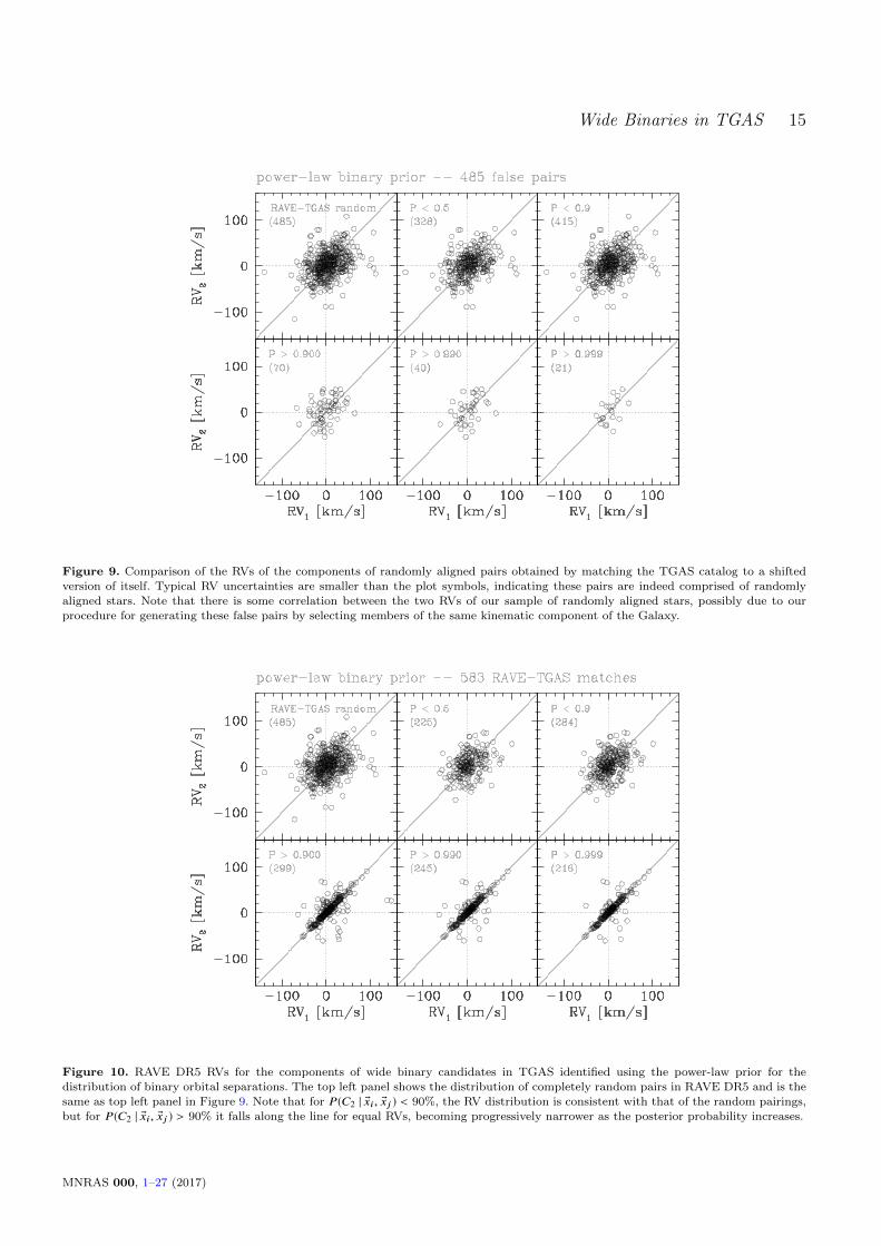
In Figure 9, we compare the RVs of each star in thesample of random alignments generated using the power-law prior for the orbital separation distribution. The typicalRV uncertainties are smaller than the plot symbols; clearlythese pairs have inconsistent RVs. Figure 9 shows some non-zero covariance in the distribution of samples.7 Also, wenote that matching RVs is a necessary but not sufficientindicator of any particular pair being a genuine binary: Fig-ure 9 shows that ≈20% of randomly aligned stellar pairs withP(C2 | ®xi, ®xj ) > 99% happen to have RVs consistent at the 3σlevel.

In Figure 10 we show, plotted against each other, theRAVE RVs for 583 pairs from our 17,895 candidate widebinaries obtained using the power-law prior. We divide theposterior probability P(C2 | ®xi, ®xj ) into five bins and give thenumber of pairs in each bin. The total number of pairs withRAVE RVs for both components is more than an order ofmagnitude larger than that identified by Oh et al. (2016) forsystems with separations <1 pc.

The sequence of panels in Figure 10 shows that ourcandidate pairs progressively align along the line of equalRV as P(C2 | ®xi, ®xj ) increases, unambiguously telling us thatgenuine wide binaries are being identified with increasinglyhigher confidence, and thus validating our method. The top

7 One possible reason for this may be due to our matching algo-rithm selecting members of the same kinematic component of the

Galaxy, e.g. thin or thick disk.

middle and top right panels, with P(C2 | ®xi, ®xj ) < 50% and90%, respectively, still look very similar to the plot showingrandom alignments. When restricting to P(C2 | ®xi, ®xj ) > 90%,however, the behavior is very different, and a large majorityof the 299 candidate pairs in this range have the RVs of thetwo components falling very close to the one-to-one line.

However, from our comparison between the distribu-tions in Figures 9 and 10, candidate pairs with posteriorprobabilities between 90% and 99% may still include somerandom alignments, in agreement with our conclusions whencomparing Figures 4 and 6. Therefore, to the limits of theavailable data, selecting candidates with P(C2 | ®xi, ®xj ) > 99%is likely to result in the purest sample of genuine wide bina-ries.

Figure 11 is the same as Figure 10, but for 863 pairsfrom our 33,169 candidate wide binaries obtained using thelog-flat prior. Again, this sample is an order of magnitudelarger than that found by Oh et al. (2016) for the samerange of separations. In general terms, the same conclusionsobtained from Figure 10 can be obtained from Figure 11,the main difference being the different relative numbers ofcandidate pairs falling in each probability range.

In the top left panel of Figure 12, we show the differencein RVs of the two stellar components from our sample of falsebinaries with RAVE RVs described in Section 5.1.2. Theseshow that the population of random alignments increases atlarge θ, and is typically of order tens of km s−1.8

Here again, the panels of Figure 12 corresponding to thecatalog from the power-law prior show the progressive nar-rowing of the distribution of pairs around the equal velocityline (in this case, ∆RV = 0) as the posterior probability in-creases, with the overall behavior being markedly differenton either side of P(C2 | ®xi, ®xj ) = 90% probability, i.e., a broaddistribution of pairs for P(C2 | ®xi, ®xj ) < 90%, and a signifi-cantly narrower one for P(C2 | ®xi, ®xj ) > 90%.

An additional difference is evident when looking at thedistributions as a function of angular separation: candidatepairs are more broadly distributed at low probabilities thanthey are at the highest ones. Visual inspection of the pan-els in the upper and lower rows in Figure 12 reveals thiswithout ambiguity. This is to be expected if the majority ofpairs with P(C2 | ®xi, ®xj ) < 90% are contamination from ran-dom alignments: the probability that two unassociated starsappear to be co-moving increases with the square of the an-gular separation. In this way, Figure 12 also argues that thecatalogs are dominated by random alignments below 90%probability, and by genuine binaries at higher probabilities.

Finally, while the assumption that the components of atrue wide binary share the same RV holds for most systems,there is one exception: the possibility that one of the com-ponents of a genuine wide binary is a (closer) binary systemitself. Such hierarchical triples or multiples are not uncom-mon among wide binaries (Makarov et al. 2008; Tokovinin2014a,b, 2015; Halbwachs et al. 2017), and the orbit of theinner subsystem can make the RVs of the components differ

8 Given that use of the log-flat prior produces more contamina-

tion at low probabilities, we focus on the catalog obtained with

the power-law prior for the distribution of orbital separations.Our conclusions are not altered if inspecting instead the catalog

obtained using the log-flat prior.

MNRAS 000, 1–27 (2017)

14 Andrews, Chaname, & Agueros

2 3 4 5 6log s (AU)

0

5

10

15

20

25

30/

Log-flat Prior / < 3/ > 3

2 3 4 5 6log s (AU)

0

1

2

3

4

5

/

2 3 4 5 6log s (AU)

0

5

10

15

20

25

30

/

Power-law Prior

2 3 4 5 6log s (AU)

0

1

2

3

4

5/

Figure 8. The distribution of proper motion differences (left panels) and parallax differences (right panels) as a function of projected

separations for binaries with P(C2 | ®xi, ®x j ) > 99% are shown as both points and greyscale contours. Blue (red) points in both panelsare those pairs in which the stars have consistent (inconsistent) parallaxes at the 3 σ level. The top panels show the sample produced

using the log-flat prior while the bottom panels show the sample produced using the power-law prior. The y axes are normalized to

their uncertainties; σ∆µ is calculated from the quadrature sum of the component uncertainties on µ∗α and µδ for both components, andσ∆$ is calculated from the quadrature sum of the individual (Gaussian) component uncertainties on $. The left panels show that many

genuine binaries exist with proper motions that differ by greater than 3 σ (horizontal line), justifying our claim in Section 2 and predicted

by Figure 1: Gaia’s astrometry is precise enough that to robustly identify wide binaries, the differential proper motion due to orbitalmotion must be accounted for. The vertical gray line is at 4×104 AU, the projected separation below which our sample is almost entirely

composed of genuine pairs, as we demonstrate in Section 5.2.

from each other when the comparison is based on a singleepoch. We further discuss this possibility, as well as othercaveats to using RAVE RVs as a calibrator for our method,in Section 5.2. For now, we note only that these exceptionsare a minority of cases, and matching the RVs of the com-ponents of a wide binary provides a satisfactory calibrationmethod for our catalogs.

5.1.3 The Critical Posterior Probability

From all the evidence just discussed, it seems adequate torequire P(C2 | ®xi, ®xj ) > 90% for a candidate pair to be reli-ably regarded as a genuine wide binary. However, our goalis to identify as clean a sample of genuine wide binaries aspossible, with no strong selection effects, and to character-

ize them as a population. Our comparison of sample dis-tances, angular separations, and projected separations forthe random alignments and our candidate binaries in Fig-ures 4 and 6 demonstrate that most of the pairs with 90%< P(C2 | ®xi, ®xj ) < 99% are random alignments. With this inmind, therefore, we require P(C2 | ®xi, ®xj ) > 99% for the widebinary samples we report and analyze in this paper.

Even at P(C2 | ®xi, ®xj ) > 99%, Figures 10, 11, and 12 showa small number of pairs that deviate significantly from theone-to-one and ∆RV = 0 lines. As pointed out earlier, thesepairs could represent contamination from chance alignmentsor be hierarchical triple systems. These should be followedup, ideally with multi-epoch RV measurements, but this isbeyond the scope of the present work.

MNRAS 000, 1–27 (2017)

Wide Binaries in TGAS 15

Figure 9. Comparison of the RVs of the components of randomly aligned pairs obtained by matching the TGAS catalog to a shiftedversion of itself. Typical RV uncertainties are smaller than the plot symbols, indicating these pairs are indeed comprised of randomly

aligned stars. Note that there is some correlation between the two RVs of our sample of randomly aligned stars, possibly due to our

procedure for generating these false pairs by selecting members of the same kinematic component of the Galaxy.

Figure 10. RAVE DR5 RVs for the components of wide binary candidates in TGAS identified using the power-law prior for thedistribution of binary orbital separations. The top left panel shows the distribution of completely random pairs in RAVE DR5 and is the

same as top left panel in Figure 9. Note that for P(C2 | ®xi, ®x j ) < 90%, the RV distribution is consistent with that of the random pairings,but for P(C2 | ®xi, ®x j ) > 90% it falls along the line for equal RVs, becoming progressively narrower as the posterior probability increases.

MNRAS 000, 1–27 (2017)

16 Andrews, Chaname, & Agueros

Figure 11. Same as Figure 10 but for the catalog of wide binary candidates identified using the log-flat prior.

Figure 12. ∆RV as a function of angular separation for the components of candidate pairs obtained using the power-law prior for thebinary separation distribution. The distributions for candidate pairs with low probability (P(C2 | ®xi, ®x j ) < 90%) are systematically widerthan those for candidates with high probabilities.

MNRAS 000, 1–27 (2017)

Wide Binaries in TGAS 17

2 3 4 5 6log s (AU)

30

20

10

0

10

20

30∆

RV/σ

∆R

V

Log-flat Prior

2 3 4 5 6log s (AU)

0

10

20

30

40

N

2 3 4 5 6log s (AU)

30

20

10

0

10

20

30

∆R

V/σ

∆R

V

Power-law Prior

2 3 4 5 6log s (AU)

0

10

20

30

40

N

Figure 13. ∆RV for the candidate TGAS wide binaries with P(C2 | ®xi, ®x j ) > 99% and RAVE matches, normalized to its uncertainty,

as a function of projected separation for both the log-flat prior (top panels) and power-law prior (bottom panels) models. Candidatepairs with ∆RV less (more) than 3σ are shown as blue (orange) points. The right two panels, which compare the projected separation

distributions, indicate that random alignments begin to dominate the overall distribution of systems at s ≈ 4 × 104 AU for both models.

Restricting for systems with projected separations smaller than this limit (shown by the gray vertical lines) substantially reduces thecontamination.

5.2 Estimating the Contamination Rate

The subset of pairs with RAVE RVs provides us with anestimate for the rate of contamination due to random align-ments. In the left two panels of Figure 13, we show thedistribution of projected separations for candidates withP(C2 | ®xi, ®xj ) > 99% as a function of their RV difference. Thisdifference is normalized by the quadrature sum of the indi-vidual RV uncertainties, σ2

∆RV = σ2RV,1 +σ

2RV,2, so that devi-

ations from zero correspond to confidence levels. Horizontallines separate those pairs with consistent RVs at the 3σ con-fidence level (blue points) from those with inconsistent RVs(orange points). The ratio of the number of candidate pairswith discrepant RVs to the overall number of candidateswith RAVE matches provides an estimate of contamination.This method assumes that the subset of our candidate bi-naries with RAVE matches is a representative sample.

The right two panels of Figure 13 show the distributionof projected separations for pairs with consistent RVs (blue)and those with discrepant RVs (orange). Contamination ex-ists at all separations, but the samples are clearly dominatedby pairs with consistent RVs out to s ≈ 4 × 104 AU. Atlarger separations, contamination begins to dominate bothsamples. Returning to the left two panels of Figure 13 and

selecting only those systems with s < 4×104 AU (delineatedby the vertical gray lines), we estimate the contaminationfraction at 17% for the log-flat prior (37/224) 16% for thepower-law prior (33/212) models.

We can obtain an additional estimate of the contami-nation fraction using our sample of random alignments. Thesample shown in Figure 4 produces approximately the samenumber of overall candidate pairs with P(C2 | ®xi, ®xj ) > 1%as our search for real wide binaries (both samples are dom-inated by random alignments with P(C2 | ®xi, ®xj ) << 99%).Restricting for those systems with P(C2 | ®xi, ®xj ) > 99% and

s < 4×104 AU, we estimate the contamination fraction usingthis method to be 6% (245/4360) and 4% (156/4024) for thelog-flat and power-law prior models, respectively.

How can the two methods for estimating the contami-nation fraction disagree so strongly for the fraction of sub-set of systems with s < 4 × 104 AU? Four factors can po-tentially make the RV-based estimate inaccurate. First, anystar in a wide binary that includes an unresolved binary canmake a genuine system appear as contamination using RVs.Makarov et al. (2008) suggest that the fraction of commonproper motion pairs that are actually higher order systemsmay be as high as 25%. However, if only 10% of the systemsin our sample were triples with an unresolved binary com-

MNRAS 000, 1–27 (2017)

18 Andrews, Chaname, & Agueros

ponent, our contamination estimate would drop to ≈5%, inagreement with the estimate from our random alignments.

Second, a consistent RV does not guarantee binarity;even systems with RVs consistent at the 3σ level may, infact, be random alignments with similar, but slightly differ-ent RVs. Third, if the sample of candidate pairs for which wefound matches in RAVE is not a representative TGAS sam-ple, any estimate based on it may be inaccurate. Finally, ifthe RAVE RV uncertainties are somewhat underestimated,the contamination fraction would be overestimated.

Our contamination fraction estimate using randomlyaligned pairs avoids these particular uncertainties. The pro-cedure generating these false pairs is identical to thatproducing our catalog of candidate binaries. Furthermore,we find that restricting for those candidate pairs withP(C2 | ®xi, ®xj ) > 99%, both the false catalog and our catalogof wide binaries produces a comparable number of systemswith s > 105 AU, supporting the idea that the false paircatalog provides a reasonable estimate of contamination forpairs with s < 4×104 AU. With these these caveats in mind,we estimate the contamination fraction to be ≈5%.

Regions 1 and 2 in Figure 6, outlined by the green andblue boxes, are designed to produce subsets of P(C2 | ®xi, ®xj ) >99% pairs within defined ranges of distances D and angularseparations that have very low contamination. Limited to10′′ < θ < 100′′ and D < 500 pc, Region 1 takes advantage ofthe large sample of genuine binaries at smaller separations.Region 2 is confined to a distance of 100 pc, while extendingto 10′ to test the distribution of binaries at relatively widerseparations. We estimate the contamination by counting thenumber of random alignments falling in these regions. Forthe log-flat prior model, our random alignment test gener-ates 135 false pairs in Region 1 and four false pairs in Region2, whereas our search identifies 2704 and 461 candidate pairsin these regions. This corresponds to contamination ratesof ≈5% and 1%, respectively. For the power-law prior, thesame test results in nearly identical contaminations ratesof ≈4% and 1% for the two regions (89/2498 4/458). It isfrom these minimally contaminated subsets that we deriveour constraints on the orbital separation distribution of widebinaries.

6 RESULTS

6.1 The TGAS Catalog of Wide Binaries

We define wide binaries as systems with a posterior prob-ability above 99% for either the log-flat or the power-lawprior model, and our final catalog of 6196 pairs is the unionof these two samples. The posterior probabilities may dif-fer substantially between the models, particularly at large swhere the differences in the prior distributions is strongest.

We note that the posterior probabilities are derivedfrom a calibrated and validated but ultimately imperfectmodel; pairs with P(C2 | ®xi, ®xj ) > 99% may still be contam-

inating objects. Indeed, at separations s & 4 × 104 AU, wesuspect most pairs are random alignments regardless of theirprobability. We discuss this possibility further in Section 7.3.Nevertheless, we include these systems in the catalog: theydefine the locus of random alignments, and there are likely

Sou

rceID

Tych

o-2

IDα

1δ1

µ ∗α,1

µδ,1

$1

Source

IDT

ych

o-2

IDα

2δ2

µ ∗α,2

µδ,2

$2

P(C2 | ®xi , ®x

j )P(C

2 | ®xi , ®xj )

θ

[mas

yr −1]

[mas

yr −1]

[mas]

[mas

yr −1]

[mas

yr −1]

[mas]

log-fl

at

pow

er-law[”]

384307763771387776

2789-1

319-1

00:0

0:1

0.1

1+

41:5

1:4

2.2

2-7

.34

-4.5

71.2

1384313742365860992

2789-1

122-1

00:0

0:4

6.5

3+

42:0

0:3

7.4

3-6

.46

-4.3

11.7

21.0

0.0

672.0

2765217352391138688

594-1

34-1

00:0

0:1

3.6

2+

09:4

7:5

6.4

326.8

2-2

.38

2.8

2765236731283414784

594-8

1-1

00:0

0:0

8.2

8+

09:5

6:0

5.5

027.4

7-1

.72

2.8

0.0

0.9

973

495.4

2305900664854805632

7526-3

20-1

00:0

0:2

0.5

5-4

1:0

2:2

7.7

748.7

-8.9

66.2

82305905578297389312

7526-5

15-1

00:0

1:3

9.2

2-4

0:5

3:2

6.6

249.4

6-7

.99

5.3

10.9

998

1.0

1042.4

429342935412328704

4014-3

283-1

00:0

0:2

6.0

6+

60:2

5:3

9.5

128.7

411.8

410.2

1429343004131805568

4014-1

005-1

00:0

0:2

4.8

3+

60:2

5:3

1.2

828.1

111.4

910.2

81.0

1.0

12.3

2880169678167998336

2271-9

11-1

00:0

0:4

9.6

6+

36:4

6:4

8.0

2-2

4.5

9-2

2.2

76.8

22880169884326428672

2271-1

988-1

00:0

0:4

8.6

2+

36:4

6:3

8.9

4-2

5.7

8-2

3.1

47.0

91.0

1.0

15.4

393882207946562176

3254-5

69-1

00:0

0:5

9.4

3+

49:5

0:5

4.4

66.0

54.7

72.7

5393882311025775616

3254-1

352-1

00:0

0:5

8.9

7+

49:5

2:0

2.1

07.0

24.1

32.0

90.9

979

0.9

864

68.7

4702974002115657472

9137-1

774-1

00:0

1:1

7.6

1-7

0:1

1:1

2.2

865.4

5-1

2.9

34.6

74702974002115657600

9137-1

708-1

00:0

1:2

2.5

0-7

0:1

1:2

6.9

365.6

1-1

3.5

44.6

11.0

1.0

28.2

531236430303749120

4298-5

98-1

00:0

1:1

8.6

6+

70:5

5:4

4.0

7-5

.31

-7.7

3.1

9531236670821917568

4298-5

74-1

00:0

1:0

3.4

5+

70:5

5:4

7.5

5-4

.8-6

.92

3.4

40.9

988

0.9

927

74.6

2738660435728687872

1-1

016-1

00:0

1:4

2.4

0+

01:4

7:1

2.5

1-1

9.2

1-2

6.3

42.6

62738660882405286272

1-1

68-1

00:0

1:4

1.5

6+

01:4

8:2

4.4

1-1

9.6

7-2

5.1

42.2

60.9

998

0.8

704

73.0

2848236321444116352

1729-1

129-1

00:0

2:0

1.7

6+

23:4

6:5

1.1

326.9

95.6

55.0

42848423994335483264

1729-1

118-1

00:0

1:5

9.8

6+

23:4

7:0

1.7

724.4

46.3

45.1

71.0

1.0

28.1

Table

2:

The

first

10

wid

ebin

aries

from

our

cata

log.

We

prov

ide

the

Gaia

source

IDs,

astro

metry,

posterio

rpro

babilities

for

both

the

log-fl

at

prio

rand

pow

er-lawprio

rm

odels,

and

angula

rsep

ara

tion.

This

table

isava

ilable

onlin

ein

itsen

tirety.

MNRAS 000, 1–27 (2017)

Wide Binaries in TGAS 19

10 4

10 3

10 2

dN/d

log

s

Log-flat Prior

D < 100 pc100 pc < D < 200 pc

102 103 104 105

s (AU)

10 4

10 3

10 2

dN/d

log

s

Power-law Prior

100

101

102

100

101

102

Num

ber o

f Pai

rs100

101

102

100

101

102

Num

ber o

f Pai

rs

Figure 14. The s distribution of our binary samples identifiedusing both the log-flat prior (top panel) and the power-law prior

(bottom panel). The left axis shows these distributions normal-

ized to the total number of TGAS stars within the distance rangeslisted, while the right axis shows the overall numbers. Background

lines show the power-law P(s) ∝ s−1.6, which decreases at larger

s. These lines are not fits to the distribution, but rather the nor-malization is scaled arbitrarily to compare the distribution to the

power-law model at large separations. Regardless of the assumed

prior, there is a drop off in the number of binaries with s >∼ 3×103

AU. The excess at 105 AU is due to random alignments, as can

be seen in the right panels of Figure 6; contamination is expectedas the distance increases, which is why the excess observed in the

sample with 102 < D < 2 × 102 pc (red) is not observed in pairs

within 102 pc (black).

to be genuine pairs within this sample that can be extractedwith a more focused analysis.

We present our catalog in Table 2. When individualstars match to multiple companions, each pair is listed as aseparate binary; we do not use these systems when determin-ing the wide binary orbital separation distribution (Sections6.2 and 6.3). We provide the Gaia source IDs, Tycho-2 sourceIDs, positions, proper motions, and parallaxes of the com-ponents of each system, the posterior probabilities of eachbinary being composed of a genuine pair, and their angularseparation.

6.2 The Orbital Separation Distribution of WideBinaries

In Figure 14, we show the distribution of projected physicalseparations for subsets of pairs within two different distancelimits for our log-flat and power-law prior models. These dis-tributions are normalized to the total number of TGAS stars

within the listed distance ranges. The small angle limit9 forour sample leads to an excess of systems at s ≤ 2 × 102 AUwithin 102 pc (black) compared with our more distant sam-ple (red). Importantly, the more distant binaries show anexcess at s ≈ 105 AU that is unseen in the closer sample atdistances ≤ 102 pc. This excess at large separations has beenobserved in other wide binary samples (Dhital et al. 2010;Oelkers et al. 2016) and suggested to be a characteristic ofthe Galactic wide binary population.

Were this increase a genuine characteristic of wide bi-naries, it should be seen in the distributions shown in Fig-ure 14 of both the samples within 102 pc and that at dis-tances between 102−2 × 102 pc. Comparison between Fig-ures 4 and 6 as well as the RV matching shown in Figure13 demonstrates that this increase occurs at the separationwhere random alignments dominate the sample. We con-clude that the relative flattening and subsequent apparentexcess of the distribution at s ≈ 4 × 104 AU in systems with102 < D < 2×102 pc corresponds to the transition from gen-uine binaries to random alignments seen in the right panelsof Figure 6. In particular, our data imply that the previouslyreported bimodality within separations of 1 pc in samples ofwide binaries (Dhital et al. 2010; Oelkers et al. 2016) is mostlikely due to contamination from random alignments.

Additionally, the distribution of projected separationsof our wide binaries, regardless of our assumed orbital sep-aration prior, is in conflict with that found by Oh et al.(2016), who report an increasing distribution of co-movingpairs with s ranging from a few 103 AU to several pc. How-ever, our sample is in agreement with CG04 and Lepine &Bongiorno (2007), both of who find samples of wide binariesdecreasing at separations larger than a few 103 AU. A ma-jor advantage of our sample over that of Oh et al. (2016) isthat we explicitly identify and estimate the contaminationfraction; after removing potential contamination our cleanedsample is nearly two orders of magnitude larger than that ofOh et al. (2016) for pairs with projected separations smallerthan 4 × 104 AU. If these authors introduced a strong se-lection function that distorts the observed distribution ofstellar pairs, the difference between their sample and ourscan be resolved.

Oh et al. (2016) further identify a set of co-movingpairs with s & 1 pc, speculating that these may be the un-bound remnants of ionized binaries whose components dis-perse in phase space during their orbital evolution. As Jiang& Tremaine (2010) demonstrate, such co-moving pairs maybe prevalent in the nearby Galaxy. We discuss the nature ofthe population of pairs with separations s & 1 pc in Section7.3; for now we note that the distribution of wide binariesreported by Oh et al. (2016) increases in the same way as apopulation of purely random pairs, a sign of potential con-tamination.

Our sample of wide binaries shows a sharp cutoff atseparations of a few 105 AU. This corresponds to the limitsimposed by our binary model defined in Section 2: based onthe expectation that (gravitationally bound) binaries do notsurvive for long at orbital separations beyond the Galactic

9 Although our catalog of wide binaries contains pairs with sep-arations as small as 2′′, Figure 7 shows there is a substantial

observational bias in effect at θ < 10′′.

MNRAS 000, 1–27 (2017)

20 Andrews, Chaname, & Agueros

tidal limit, our model has a strict upper limit that a ≤ 1 pc.As noted earlier, binaries with separations >1 pc may existand indeed have been identified (e.g., CG04; Shaya & Olling2011). However, our results indicate that correctly identify-ing such widely separated systems as genuinely associatedpairs is very challenging.

The dotted lines in Figure 14 correspond to the power-law distribution observed by CG04 and Lepine & Bongiorno(2007) with P(s) ∝ s−1.6. These lines are scaled verticallyto compare the distribution to the power-law model at largeseparations. Random alignments artificially increase the dis-tribution at large s for the pairs with 102 < D < 2 × 102 pc.Because the D < 102 pc sample has less contamination atlarger s, the power-law provides a reasonable model from≈5×103 to 105 AU. In the following section, we demonstratethat this decrease at large s cannot be due to observationalbiases in detecting binaries with large θ. The distribution ofs is clearly inconsistent with Opik’s Law for s >∼ 104 AU, andit is not bimodal for s . 1 pc.

6.3 Comparison to Models

To go beyond our by-eye comparison to the power-law sep-aration distribution shown in Figure 14, we wish to useour full catalog of 6196 systems with posterior probabili-ties above 99%. The interdependence of distance, projectedseparation, and angular separation of these binaries shownin the right panels of Figure 6 demonstrates the difficulty inderiving the underlying distribution of physical separations.Contamination at large s, bias introduced by the distancedistribution of stars in TGAS, and the angular resolutionlimit of TGAS at small s may all cause inaccuracies whendetermining the distribution of s. Our approach is to gen-erate a sample of synthetic wide binaries from an arbitrarybinary population model, convert those binaries to an angu-lar separation distribution, P(θ), accounting for the angularseparation limits and distance dependence of TGAS. In thisway, we are calculating P(θ) as predicted by the models todirectly compare to subsets of our sample of binaries.

We restrict ourselves to Regions 1 and 2, defined inFigure 6, to calculate P(θ) expected from the model by inte-grating over the two oblique regions in D-s space and thenfactoring terms based on independence:

P(θ) = Z∫ Dmax

0

∫ smax

smindD ds P(θ,D, s)

= Z∫ Dmax

0

∫ smax

smindD ds P(θ | D, s) P(D) P(s),(38)

where Z is an integration constant to normalize the prob-ability and smin and smax are the minimum and maximumprojected separations, respectively, to which we are sensi-tive. For a given distance, these are limited by our angularseparation constraints: at the close end by the angular sen-sitivity of the Tycho-2 catalog and at the distant end by oursearch radius of 100′′ for Region 1 and 10′ for Region 2.

Since θ can be expressed as a function of D and s, Equa-tion 38 can be reduced by substituting a Dirac delta functionfor P(θ | D, s):

P(θ) = Z∫ Dmax

0

∫ smax

smindD ds δ

[θ − s

D

]P(D) P(s). (39)

The delta function reduces the inner integral over s. Afterdividing by the Jacobian term, 1/D, which comes from thederivative of the argument of the delta function, Equation39 becomes:

P(θ) = Z∫ Dmax

0dD D P(D) P(s∗), (40)

where s∗ = θD. P(D) is the distance distribution of oursample of binaries, and P(s∗) depends on the specific bi-nary model used. We determine P(D) empirically by gen-erating a KDE from the subsample of our binaries with5 × 103 < s < 5 × 104 AU. This sample should be free ofbiases imposed by the TGAS angular separation limits andof contamination from random alignments at large s.

To generate P(s), we create 105 binaries with randomlychosen orbital parameters and calculate the projected phys-ical separation in the same way as described in Section 3.3.A thermal eccentricity distribution is assumed. Again, wegenerate P(s) for two models, one with a log-flat distribu-tion for the orbital separation in the range 10 R�−1 pc, andone with a power-law of index −1.6. We approximate eachof these distributions of 105 random binaries with gaussianKDEs to generate P(s).

The integral in Equation 40 is normalized over the entirerange of θ. To obtain P(θ) over the range to which we aresensitive, we need to calculate the integration constant Z:

Z−1 =

∫ θmax

θmindθ P(θ), (41)

where θmin and θmax are the angular separation limits defin-ing the region to which we are sensitive. To avoid incom-pleteness at small separations and random alignments atlarge separations, we set θmin to 10′′ and θmax to 10′ forRegion 1 and θmax to 100′′ for Region 2.

We compare the actual P(θ) for binaries in our two sam-ples to these distributions. For both the log-flat and power-law distributions, we find P(θ) by numerically calculatingthe integral in Equation 40. Each panel in Figure 15 com-pares P(θ) for each of these two models. The top row of pan-els shows the distributions for our sample using the power-law model as our binary population prior, while the bottompanel shows that for the log-flat prior. The two columnscompare the distributions for Region 1 extending to 10′ and100 pc and Region 2 extending to 100′′ and 500 pc.

The left panels in Figure 15, calculated using those bi-naries in Region 1, focus on the distributions of pairs withsmall θ. Although the two samples are very similar at theseseparations, the number of binaries in our sample allow usto discern between the two models. For θ <∼ 80′′, the popu-lation starts to have a shallower slope, closer to the log-flatdistribution. This indicates that the turnover observed atseparations of ≈5 × 103 AU in Figure 14 is genuine.

The right two panels, calculated for binaries in Region2, show that, regardless of the binary population model as-sumed, at separations out to 300′′ the observed populationmatches the power-law distribution. Beyond 300′′, the distri-bution deviates slightly, which may be due to the increasedimportance of random alignments (however, the uncertain-ties at separations beyond 300′′ are large). At smaller angu-lar separations, the two models overlap.

Importantly, our results are identical regardless of thepriors we use: both models show that P(s) should be roughly

MNRAS 000, 1–27 (2017)

Wide Binaries in TGAS 21

10 3

10 2

10 1

Nor

mal

ized

Pro

babi

lity

Log-flat Prior

Region 1

10 4

10 3

10 2

10 1

Nor

mal

ized

Pro

babi

lity

Log-flat Prior

Region 2

10 20 30 40 50 60 70 80 90 100 (")

10 3

10 2

10 1

Nor

mal

ized

Pro

babi

lity

Power-law Prior

100 200 300 400 500 600 (")

10 4

10 3

10 2

10 1

Nor

mal

ized

Pro

babi

lity

Power-law Prior

Figure 15. P(θ) for two models: one based on Opik’s Law, in which a is selected randomly from a log-flat distribution (dotted lines), and

one with a power-law distribution (dashed lines). P(θ) in both cases is calculated using the method outlined in Section 6.3. We comparethese models to the two different samples of pairs we generate, one using the log-flat prior (top panels) and one using the power-law prior

(bottom panels). The left and right columns of panels are computed for Regions 1 and 2, respectively, shown in Figure 6 and described

in Section 6.2. In every panel, we compare our samples to the two model distributions. Regardless of the prior distribution assumed,our model robustly indicates that at larger separations, θ corresponds to a power-law steeper than flat and consistent with P(s) ∝ s−1.6,

while at smaller separations the distribution flattens out and is consistent with a log-flat distribution.

log-flat at small separations and scale with roughly s−1.6

at large separations. These results are consistent with theresults of CG04 and Lepine & Bongiorno (2007), both ofwhom, using independent samples, find a flattening of thedistribution at small s. For instance, Lepine & Bongiorno(2007) determines that P(s) ∝ s−1 for s < 2500 AU while atlarger separations, P(s) ∝ s−1.6; for θ < 10′′, the log-flat andpower-law distributions diverge further. Future Gaia datareleases will be sensitive to these differences.

7 DISCUSSION

7.1 Comparison with Pre-Gaia Wide BinarySamples

Searches of proper-motion catalogs for wide binaries haveused different astrometric catalogs and were therefore sen-sitive to different samples of wide binaries. We briefly sum-marize the work of several of these groups before comparingtheir samples to that identified in this work.

CG04 searched the rNLTT catalog, a reanalysis of starsin the NLTT catalog (Salim & Gould 2003), to identify widebinaries among common proper motion pairs. The stars in

this catalog extend to V ≈ 19 mag; the relative proper motionsensitivity is ≈3 mas yr−1.

Lepine & Bongiorno (2007) searched for common propermotion companions to Hipparcos stars in the LPSM-Northcatalog, a catalog identified using a reanalysis of the starsin the Digitized Sky Survey and containing stars with µ >

0.15′′ yr−1 (Lepine & Shara 2005). Since the primary starsare found in Hipparcos data, this catalog contains the bright-est and nearest stars.

Dhital et al. (2010) searched SDSS for common propermotion pairs containing low-mass stars. Proper motions areprovided by the SDSS team by comparing to photometricplates from the USNO-B and POSS-II surveys (Munn et al.2004). The digital nature of SDSS and the long time baselineresults in proper motions with precisions ≈few mas yr−1 forstars as faint as g ≈ 20 mag. However, this sample is limitedby several factors: source confusion prevents pairs with an-gular separations .7′′ from being identified and SDSS hasa bright limit of g ≈ 14 and limited sky coverage.

Finally, Shaya & Olling (2011) searched the Hippar-cos catalog for wide binaries. This sample includes onlythe brightest pairs, since the Hipparcos catalog is limited toV . 9 mag; however, the resulting catalog extends to proper

MNRAS 000, 1–27 (2017)

22 Andrews, Chaname, & Agueros

10 1

100

101

102

103

104

Prop

er M

otio

n (m

as y

r1 )

N = 1148

Chaname & Gould (2004)

N = 552

Lepine & Bongiorno (2007)

N = 1342

Dhital et al. (2010)

N = 543

Shaya & Olling (2011)

N = 6197

This work

100 101 102 103 104

Angular Separation (")

2468

10121416182022

Appa

rent

Mag

nitu

de

V mag

100 101 102 103 104

Angular Separation (")

V mag

100 101 102 103 104

Angular Separation (")

SDSS g mag

100 101 102 103 104

Angular Separation (")

V mag

100 101 102 103 104

Angular Separation (")

Gaia g mag

Figure 16. The two panels in each column show the distribution of angular separations, proper motions, and magnitudes for four

samples of wide binaries in the literature and for the sample identified in this work. While previous catalogs were limited to nearby pairswith large proper motions, the TGAS astrometric precision allows us to identify binaries with proper motions down to a few mas yr−1.

However, the photometric limitations of the Tycho-2 catalog result in the pairs identified in this work being relatively brighter than

previously identified pairs (with the exception of the catalog of Shaya & Olling 2011, which is based on stars with Hipparcos astrometry).Future Gaia data releases should allow us to extend this sample to fainter magnitudes. Note that the magnitudes shown are in the bands

provided in the respective catalogs.

motions as small as a few mas yr−1. Shaya & Olling (2011)were able to identify such slowly moving pairs because theiralgorithm also matched stars based on Hipparcos parallaxes.

The left four columns in Figure 16 compares the angularseparations, magnitudes, and proper motions of pairs iden-tified in the catalogs of CG04, Lepine & Bongiorno (2007),Dhital et al. (2010), and Shaya & Olling (2011).10 The rightcolumn shows the distributions for the wide binaries identi-fied in this work. The bottom panel in the rightmost columndemonstrates that, like for Shaya & Olling (2011) and Lepine& Bongiorno (2007), our pairs tend to be at brighter mag-nitudes (Gaia g . 11 mag), reflecting the relatively brightfaintness limit of the Tycho-2 catalog. However, even moreso than Shaya & Olling (2011), we are identifying pairs withsmaller proper motions.

The number of pairs in each catalog is provided in thetop panel of each column. Our catalog represents an increasein size of a factor of ≈5-10 over each of the previous catalogs.At the same time, the CG04 and Dhital et al. (2010) catalogsshown in Figure 16 indicate that many more pairs exist withfainter magnitudes and large proper motions. Therefore, wecan infer that the sample of wide binaries identified in thiswork represents a small subset of a much larger populationthat will be identified in future Gaia data releases.

10 We only include those pairs identified by Shaya & Olling (2011)

with a probability above 50%.

7.2 The Impact of Our Assumptions

We discuss two of the three most important assumptions wemade in constructing our catalog: the prior on the parallaxand the binary fraction. The other assumption, about theinput binary population model, was discussed in Section 3.3.

7.2.1 The Prior on the Parallax

Through their analysis of individual stars, Astraatmadja &Bailer-Jones (2016) test several prior distributions on par-allax. These authors identify a model with an exponentiallydecreasing density with a scale length of 1.35 kpc as a reason-ably accurate description of the parallax distribution. Thisis the prior we use, and we provide its functional form inSection 3.3.

As discussed by Lutz & Kelker (1973) and confirmed forGaia data by Astraatmadja & Bailer-Jones (2016), the astro-metric parallax is a poor measure of distance when its frac-tional uncertainty, σ$/$, is >∼20%. Stars with small σ$/$(which are usually closer by) are less sensitive to the assumedparallax prior. Since the typical TGAS σ$ ≤ 0.3 mas, theparallaxes should be accurate for stars within <∼700 pc, whichdescribes the vast majority of our wide binaries.

We test this assumption by running our algorithm withan empirically motivated parallax model based on the dis-tribution of observed parallaxes. Specifically, we generate aKDE of a subset of parallaxes in the TGAS catalog to ap-proximate this distribution. Uncertainties will tend to makea population of stars with small parallaxes appear somewhatcloser, and therefore to have larger parallaxes, than at their

MNRAS 000, 1–27 (2017)

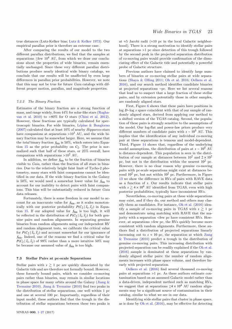
Wide Binaries in TGAS 23

true distances (Lutz-Kelker bias; Lutz & Kelker 1973). Ourempirical parallax prior is therefore an extreme case.

After comparing the results of our model to the twodifferent parallax distributions, we find that the samples atseparations <∼few 104 AU, from which we draw our conclu-sions about the properties of wide binaries, remain essen-tially unchanged. Since these very different parallax distri-butions produce nearly identical wide binary catalogs, weconclude that our results will be unaffected by even largedifferences in parallax prior probabilities. However, we notethat this may not be true for future Gaia catalogs with dif-ferent proper motion, parallax, and magnitude properties.

7.2.2 The Binary Fraction

Estimates of the binary fraction are a strong function ofmass, and range widely, from 44% for solar-like stars (Ragha-van et al. 2010) to >80% for O stars (Chini et al. 2012).However, these fractions are typically calculated for spec-troscopic binaries. For wide binaries, Lepine & Bongiorno(2007) calculated that at least 10% of nearby Hipparcos starshave companions at separations >103 AU, and the wide bi-nary fraction may be somewhat larger. Here, we assume thatthe total binary fraction fbin is 50%, which enters into Equa-tion 15 as the prior probability on C2. The prior is nor-malized such that half of these stars, or 25% overall, havecompanions with separations >102 AU.

In addition, we define fbin to be the fraction of binariesvisible to Gaia, rather than the fraction of all stars in bina-ries. Due to the relatively bright faint limit of Tycho-2 pho-tometry, many stars with faint companions cannot be iden-tified in our data. If the wide binary fraction in the Galaxyis 50%, we would need a somewhat lower value for fbin toaccount for our inability to detect pairs with faint compan-ions. This bias will be substantially reduced in future Gaiadata releases.

Fortunately, there is some freedom in our model to ac-count for an inaccurate value for fbin, as it scales monoton-ically with our posterior probability P(C2 | ®xi, ®xj ) in Equa-tion 15. If our adopted value for fbin is too high, it willbe reflected in the distribution of P(C2 | ®xi, ®xj ) for both gen-uine pairs and random alignments. In separating genuinebinaries from random alignments using our independent RVand random alignment tests, we calibrate the critical valuefor P(C2 | ®xi, ®xj ) and account somewhat for our ignorance offbin. Indeed, one of the reasons we find a critical value forP(C2 | ®xi, ®xj ) of 99% rather than a more intuitive 50% maybe because our assumed value of fbin is too high.

7.3 Stellar Pairs at pc-scale Separations

Stellar pairs with s & 1 pc are quickly dissociated by theGalactic tide and are therefore not formally bound. However,these formerly bound pairs, which we consider co-movingpairs rather than binaries, may remain in similar locationsin phase space for many orbits around the Galaxy (Jiang &Tremaine 2010). Jiang & Tremaine (2010) find two peaks inthe distribution of stellar separations, one well within 1 pcand one at several 100 pc. Importantly, regardless of theirinput model, these authors find that the trough in the dis-tribution of stellar separations between these two peaks is

at ≈5 Jacobi radii (≈10 pc in the local Galactic neighbor-hood). There is a strong motivation to identify stellar pairsat separations >1 pc since detection of this trough followedby the second peak in the projected separation distributionof co-moving pairs would provide confirmation of the disso-ciating effect of the Galactic tide and potentially a powerfulprobe of Galactic structure.

Previous authors have claimed to identify large num-bers of binaries or co-moving stellar pairs at wide separa-tions (Shaya & Olling 2011; Oh et al. 2016; Oelkers et al.2016), and our search method identifies candidate binariesat projected separations ∼pc. Here we list several reasonsthat lead us to suspect that a large fraction of these stellarpairs, and by extension potentially those in other samples,are randomly aligned stars.

First, Figure 6 shows that these pairs have positions inlog D−log s space coincident with that of our sample of ran-domly aligned stars, derived from applying our method toa shifted version of the TGAS catalog. Second, the popula-tion of these pairs is strongly sensitive to the assumptions ofthe model. Our log-flat and power-law priors produce verydifferent numbers of candidate pairs with s ∼ 105 AU. Thisimplies that the identification of any individual co-movingpair at these separations is tenuous and model-dependent.Third, Figure 14 shows that, regardless of the underlyingmodel assumptions, the distribution of pairs at s ∼ 105 AUis distance-dependent. This population is seen in the distri-bution of our sample at distances between 102 and 2 × 102

pc, but not in the distribution within the nearest 102 pc.However, there is no clear reason why genuine co-movingpairs with pc-scale separations might exist at distances be-yond 102 pc, but not within 102 pc. Furthermore, in Figure13 we show the difference in RVs of pairs with RAVE dataas a function of s. Our results indicate that stellar pairswith s & 4 × 104 AU identified from TGAS, even with highposterior probabilities, typically have inconsistent RVs.

Nevertheless, co-moving pairs at these wide separationsmay exist, and if they do, our method and others may clas-sify them as candidates. For instance, Oh et al. (2016) iden-tify a sample of co-moving pairs in TGAS with s & 1 pcand demonstrate using matching with RAVE that the ma-jority with a separation <few pc have consistent RVs. How-ever, at separations >few pc, the RVs quickly become moreconsistent with random alignments. Furthermore, these au-thors find a distribution of projected separations linearlyincreasing out to s ≈ 10 pc, the separation at which Jiang& Tremaine (2010) predict a trough in the distribution ofgenuine co-moving pairs. This increasing distribution withprojected separation can be readily explained if the Oh et al.(2016) sample is dominated at these separations by ran-domly aligned stellar pairs: the number of random align-ments increases with phase space volume, and therefore lin-early with projected separation.

Oelkers et al. (2016) find several thousand co-movingpairs at separations >1 pc. As these authors estimate con-tamination based on an assumed Galactic model rather thana data-driven, independent method such as matching RVs,we suggest that at separations >∼4 × 104 AU random align-ments may be a significant source of contamination in theircatalog, similar to what we see in our data.

Identifying wide stellar pairs that cluster in phase space,as is done by Oh et al. (2016), may be effective for detecting

MNRAS 000, 1–27 (2017)

24 Andrews, Chaname, & Agueros

co-moving stellar conglomerations such as triple or highermultiplicity systems, open clusters, OB associations, andmoving groups. However, the analysis we perform indicatesthat at separations beyond ∼1 pc it becomes increasinglydifficult to separate isolated co-moving pairs from randomlyaligned stars. We suggest that future searches for such pairsinclude careful accounting for contamination and, if possible,validation with RVs.

7.4 Using this Catalog

Before using the catalog provided in Table 2 there are anumber of caveats to consider. First, the immense majorityof pairs with posterior probabilities >90% are likely to berandom alignments, and our results are derived from onlythose systems with posterior probabilities >99%. Neverthe-less, there may be some contaminating random alignmentsin this sample. As discussed in Sections 5.1.1 and 5.1.2, ran-domly aligned pairs typically have s > 4 × 104 AU, whilepairs with s < 4 × 104 AU are mostly genuine.

However, the transition between genuine pairs and ran-dom alignments is not sharp; genuine pairs with s > 4 ×104 AU likely exist in our catalog, as may random align-ments with very small separations. In particular, Figure 4shows that random alignments may have angular separationsas small as 1′′. To obtain a large and pure sample, we suggestusing the subset of our candidate pairs in which the power-law posterior probability is above 99% and s < 4 × 104 AU.Based on the tests described in Section 5.1.2, we expect thecontamination of such a sample to be <∼5%.

Contamination due to random alignments becomes evenless problematic for the candidate pairs falling within Re-gions 1 and 2 in Figure 6. Contamination is nearly non-existent for pairs in Region 2 in particular. However, thesedata are subject to important observational biases, partic-ularly in distance. When deriving sample statistics wheresensitivity to distance may be relevant, this bias should betaken into account. In Section 6.3, we describe one methodfor taking this into account using a Bayesian formalism.

Although we do not expect any bias in terms of θ to existat separations larger than 10′′, Figure 7 shows a markeddecrease in the number of stellar pairs with θ < 10′′.

8 CONCLUSIONS

8.1 Summary of Results

We present a method to identify wide binaries by matchingpairs of stars based on their positions, proper motions, andparallaxes. We make no effort to identify co-moving stars instellar clusters, moving groups, or higher multiplicity sys-tems. We use a fully Bayesian method to discern betweenrandomly aligned double stars and genuine binaries. Uncer-tainties on the astrometric quantities as well as their covari-ances are properly included in our analysis. We argue (andconfirm using our resulting sample) that Gaia’s astromet-ric precision is fine enough to identify small differences inthe proper motions of stars in wide binaries due to orbitalvelocity. We account for these slight velocity differences inour search algorithm. Furthermore, our method makes no

assumptions about the structure of the Galaxy, and we cal-ibrate it using independent RV observations.

As a test, in Appendix A we apply our algorithm tothe subset of the revised NLTT catalog with parallaxesmeasured by Hipparcos (Gould & Salim 2003). Chaname &Gould (2004), whose search algorithm did not include par-allax, identify 44 wide binaries in this sample. We re-detectthese 44 binaries and find an additional 72 new wide bina-ries. This test demonstrates both the discerning power ofincluding parallax as a matching criterion and the successof our method at parsing catalogs to identify wide binaries.

After applying our method to the 2×106 stars in theTGAS catalog, we identify 6196 wide binaries with a pos-terior probability above 99% in at least one of the catalogsproduced using our two prior probability distributions forthe orbital separation. Matching stars in our pairs with theRAVE catalog provides a subsample of our catalog that haveRVs for both components. These RVs provide a test for ourmethod: widely separated but gravitationally bound bina-ries should have components with matching RVs (modulothe presence of hierarchical triples). This test indicates thatour catalog has a high fidelity and is largely free of unasso-ciated, randomly aligned pairs.

When compared to catalogs of previously identifiedwide binaries, the pairs in this catalog are typically brighter,due to the magnitude limits of the Tycho-2 catalog. Never-theless, our pairs extend to much smaller proper motions;where previous wide binary catalogs only include binarieswith large proper motions, our sample contains binaries withproper motions as small as a few mas yr−1.

Our sample suffers from strong biases at both small sep-arations, due to the angular separation limits of the Tycho-2catalog, and at large angular separations, where contami-nation from randomly aligned pairs dominates the sample.Nevertheless, we define a method to compare an arbitrarydistribution of binary separations with our biased sample.

Our sample indicates that at large physical separations,the distribution of binaries follows roughly a power-law withan index of −1.6, in agreement with the wide binary distri-butions identified by both Chaname & Gould (2004) andLepine & Bongiorno (2007). At smaller separations, the dis-tributions flatten to a power-law index closer to −1 (Opik’sLaw). Importantly, these results are robust, as they are inde-pendent of whether our model assumes a log-flat or a power-law distribution as a prior on the orbital separation. A largersample at a wider range of angular separations is needed tobetter determine the exact shape of this distribution.

Finally, we do not find a bimodality in the separations,as reported by previous authors (Dhital et al. 2010; Oelk-ers et al. 2016). Using RVs and comparing our catalog toa sample of random alignments, we demonstrate that themajority of candidate pairs identified by our method withs & 4 × 104 AU are composed of randomly aligned, unasso-ciated stars. We nevertheless include these pairs in our cat-alog, since a more focused analysis may be able to extractgenuine binaries and co-moving pairs from this sample.

Future Gaia data releases will include RVs for starsbrighter than ≈15 mag. Such measurements allow an im-portant additional constraint on the binarity of widely sep-arated pairs, potentially identifying wide binaries by match-ing their positions in full six-dimensional phase space. How-ever, stars with matching parallaxes and proper motions but

MNRAS 000, 1–27 (2017)

Wide Binaries in TGAS 25

mismatched RVs may still be associated: the pair may actu-ally be a hierarchical triple, with one star in the pair a close,unresolved binary. Engaging in RV follow-up of matchedpairs with mismatched RVs may prove to be a unique andefficient method for identifying a population of hierarchicaltriple systems.

8.2 Application to Future Gaia Data Releases

Our method is designed to take advantage of Gaia’s preciseastrometry while remaining scalable to larger data sets. Ourcurrent algorithm has a computational cost of a few 100CPU hours for the 2×106 stars in the TGAS catalog. Withmodest optimization, this algorithm should be applicable tothe 109 stars expected in the upcoming Gaia data releases.

Given the magnitude limits of the first Gaia data re-lease, the pairs identified here are likely to have mass ra-tios close to unity. We therefore postpone any discussion ofpopulation statistics in terms of stellar masses for this sam-ple. Upcoming data releases will extend the sample of starswith five-dimensional astrometry to V ≈ 20. Using the yieldsfrom previous searches for wide binaries as an indicator, weestimate that searches through these future Gaia data setswill produce 104−105 wide binaries. This population will belarge enough to identify robustly the underlying populationof wide binaries as a function of mass and ultimately testvarious models for the formation of wide binaries.

ACKNOWLEDGEMENTS

We thank the anonymous referee for helpful suggestionswhich greatly improved the manuscript. J.C. thanks Clau-dia Aguilera-Gomez for introducing him to TOPCAT, whichwas extremely useful for working with the large TGASand RAVE databases. We used the python module cor-

ner (Foreman-Mackey 2016) to produce several figures inthis manuscript. This research made use of Astropy, acommunity-developed core Python package for Astronomy(Astropy Collaboration et al. 2013). J.J.A. acknowledgesfunding from the European Research Council under the Eu-ropean Union’s Seventh Framework Programme (FP/2007-2013)/ERC Grant Agreement n. 617001. J.C. acknowledgessupport from the Chilean Ministry for the Economy, Devel-opment, and Tourism’s Programa Iniciativa Cientıfica Mile-nio, through grant IC120009 awarded to the Millenium In-stitute of Astrophysics (MAS), from PFB-06 Centro de As-tronomia y Tecnologias Afines, and from Proyecto FONDE-CYT Regular 1130373. This work has made use of data fromthe European Space Agency (ESA) mission Gaia (http://www.cosmos.esa.int/gaia), processed by the Gaia DataProcessing and Analysis Consortium (DPAC, http://www.cosmos.esa.int/web/gaia/dpac/consortium). Funding forthe DPAC has been provided by national institutions, inparticular the institutions participating in the Gaia Multi-lateral Agreement. We acknowledge use of the MetropolisHPC Facility at the CCQCN Center of the University ofCrete, supported by the European Union Seventh Frame-work Programme (FP7-REGPOT-2012-2013-1) under grantagreement no. 316165.

REFERENCES

Allen C., Monroy-Rodrıguez M. A., 2014, ApJ, 790, 158

Allen C., Poveda A., Herrera M. A., 2000, A&A, 356, 529

Andrews J. J., Agueros M. A., Belczynski K., Dhital S., Kleinman

S. J., West A. A., 2012, ApJ, 757, 170

Andrews J. J., Agueros M. A., Gianninas A., Kilic M., Dhital S.,Anderson S. F., 2015, ApJ, 815, 63

Astraatmadja T. L., Bailer-Jones C. A. L., 2016, ApJ, 832, 137

Astropy Collaboration et al., 2013, A&A, 558, A33

Bahcall J. N., Hut P., Tremaine S., 1985, ApJ, 290, 15

Bate M. R., Bonnell I. A., Bromm V., 2002, MNRAS, 336, 705

Baxter R. B., et al., 2014, MNRAS, 440, 3184

Binney J., Tremaine S., 1987, Galactic dynamics

Bonnell I. A., Bate M. R., 1994, MNRAS, 271

Chaname J., Gould A., 2004, ApJ, 601, 289

Chaname J., Ramırez I., 2012, ApJ, 746, 102

Chini R., Hoffmeister V. H., Nasseri A., Stahl O., Zinnecker H.,

2012, MNRAS, 424, 1925

Dhital S., West A. A., Stassun K. G., Bochanski J. J., 2010, AJ,139, 2566

Dhital S., West A. A., Stassun K. G., Schluns K. J., Massey A. P.,

2015, AJ, 150, 57

Duchene G., Kraus A., 2013, ARA&A, 51, 269

Duquennoy A., Mayor M., 1991, A&A, 248, 485

Elliott P., Bayo A., 2016, MNRAS, 459, 4499

Finley D. S., Koester D., 1997, ApJ, 489, L79

Fischer D. A., Marcy G. W., 1992, ApJ, 396, 178

Foreman-Mackey D., 2016, The Journal of Open Source Software,24

Fujii M. S., Saitoh T. R., Portegies Zwart S. F., 2012, ApJ, 753,

85

Gaia Collaboration et al., 2016a, A&A, 595, A1

Gaia Collaboration et al., 2016b, A&A, 595, A2

Garces A., Catalan S., Ribas I., 2011, A&A, 531, A7

Garnavich P. M., 1991, PhD thesis, Washington Univ., Saint

Louis, MO.

Gould A., Salim S., 2003, ApJ, 582, 1001

Gould A., Bahcall J. N., Maoz D., Yanny B., 1995, ApJ, 441, 200

Halbwachs J.-L., Mayor M., Udry S., 2017, MNRAS, 464, 4966

Harrison D. L., 2011, Experimental Astronomy, 31, 157

Hernandez X., Lee W. H., 2008, MNRAS, 387, 1727

Høg E., et al., 2000, A&A, 355, L27

Jiang Y.-F., Tremaine S., 2010, MNRAS, 401, 977

Kouwenhoven M. B. N., Goodwin S. P., Parker R. J., Davies

M. B., Malmberg D., Kroupa P., 2010, MNRAS, 404, 1835

Kroupa P., 1995, MNRAS, 277

Kroupa P., Aarseth S., Hurley J., 2001, MNRAS, 321, 699

Kunder A., et al., 2016, preprint, (arXiv:1609.03210)

Lada C. J., Lada E. A., 2003, ARA&A, 41, 57

Latham D. W., Schechter P., Tonry J., Bahcall J. N., SoneiraR. M., 1984, ApJ, 281, L41

Lepine S., Bongiorno B., 2007, AJ, 133, 889

Lepine S., Shara M. M., 2005, AJ, 129, 1483

Lepine S., Rich R. M., Shara M. M., 2007, ApJ, 669, 1235

Li T., Marshall J. L., Lepine S., Williams P., Chavez J., 2014, AJ,

148, 60

Lindegren L., et al., 2016, A&A, 595, A4

Longhitano M., Binggeli B., 2010, A&A, 509, A46

Lutz T. E., Kelker D. H., 1973, PASP, 85, 573

Luyten W. J., 1971, Ap&SS, 11, 49

Luyten W. J., 1979, New Luyten catalogue of stars with propermotions larger than two tenths of an arcsecond; and first sup-

plement; NLTT. (Minneapolis (1979)); Label 12 = short de-

scription; Label 13 = documentation by Warren; Label 14 =catalogue

Makarov V. V., Zacharias N., Hennessy G. S., 2008, ApJ, 687,

566

MNRAS 000, 1–27 (2017)

26 Andrews, Chaname, & Agueros

Michalik D., Lindegren L., Hobbs D., 2015, A&A, 574, A115

Moeckel N., Bate M. R., 2010, MNRAS, 404, 721

Moeckel N., Clarke C. J., 2011, MNRAS, 415, 1179

Monroy-Rodrıguez M. A., Allen C., 2014, ApJ, 790, 159

Munn J. A., et al., 2004, AJ, 127, 3034

Oelkers R. J., Stassun K. G., Dhital S., 2016, preprint,

(arXiv:1611.07883)

Oh S., Price-Whelan A. M., Hogg D. W., Morton T. D., Spergel

D. N., 2016, preprint, (arXiv:1612.02440)

Opik E. J., 1924, Tartu Obs. Publ., 25, 1

Penarrubia J., Ludlow A. D., Chaname J., Walker M. G., 2016,

MNRAS, 461, L72

Perryman M. A. C., et al., 1997, A&A, 323, L49

Poveda A., Allen C., Hernandez-Alcantara A., 2007, in Hartkopf

W. I., Harmanec P., Guinan E. F., eds, IAU Sympo-

sium Vol. 240, Binary Stars as Critical Tools & Tests inContemporary Astrophysics. pp 417–425 (arXiv:0705.2021),

doi:10.1017/S1743921307004383

Quinn D. P., Smith M. C., 2009, MNRAS, 400, 2128

Quinn D. P., Wilkinson M. I., Irwin M. J., Marshall J., Koch A.,

Belokurov V., 2009, MNRAS, 396, L11

Raghavan D., et al., 2010, ApJS, 190, 1

Reipurth B., Mikkola S., 2012, Nature, 492, 221

Rodriguez J. E., et al., 2016, AJ, 151, 123

Rojas-Ayala B., Covey K. R., Muirhead P. S., Lloyd J. P., 2010,

ApJ, 720, L113

Salim S., Gould A., 2003, ApJ, 582, 1011

Sesar B., Ivezic Z., Juric M., 2008, ApJ, 689, 1244

Shaya E. J., Olling R. P., 2011, ApJS, 192, 2

Smith Jr. H., 1987, A&A, 171, 336

Soderblom D. R., 2010, ARA&A, 48, 581

Stassun K. G., Torres G., 2016, ApJ, 831, L6

Theuns T., 1992, A&A, 259, 493

Tokovinin A., 2014a, AJ, 147, 87

Tokovinin A., 2014b, AJ, 148, 72

Tokovinin A., 2015, AJ, 150, 177

Tokovinin A., Kiyaeva O., 2016, MNRAS, 456, 2070

Tokovinin A., Lepine S., 2012, AJ, 144, 102

Wasserman I., Weinberg M. D., 1991, ApJ, 382, 149

Weinberg M. D., Shapiro S. L., Wasserman I., 1987, ApJ, 312,367

Yoo J., Chaname J., Gould A., 2004, ApJ, 601, 311

York D. G., et al., 2000, AJ, 120, 1579

Zhao J. K., Oswalt T. D., Willson L. A., Wang Q., Zhao G., 2012,

ApJ, 746, 144

de Bruijne J. H. J., Allen M., Azaz S., Krone-Martins A.,

Prod’homme T., Hestroffer D., 2015, A&A, 576, A74

van Leeuwen F., 2009, A&A, 497, 209

APPENDIX A: TESTING OUR METHOD WITHTHE REVISED NLTT CATALOG

Before applying our method to the TGAS catalog, we testedit against a set of wide binaries already identified in theliterature from an astrometric catalog: the rNLTT catalog(Gould & Salim 2003; Salim & Gould 2003), which con-tains 36,085 entries with a typical µ uncertainty of severalmas yr−1. The stars in rNLTT are mostly at latitudes aboveand below the Galactic Plane and were selected based ontheir large proper motions. Because of this low density inboth position and proper motion space, the probability ofrandomly aligned pairs is substantially smaller in rNLTTthan in TGAS.

Since our method requires parallaxes, we tested it onlyon the 8288 rNLTT stars with Hipparcos parallaxes. We

101 102 103

θ (′′)

10-1

100

101

102

103

∆µ

(mas

yr−

1)

New Pairs

Detected CG04 Pairs

102 103 104

µ (mas yr−1)

0

50

100

150

200

250

300

350

(mas)

Figure A1. The 44 wide binaries with Hipparcos parallaxes in

the CG04 catalog (black), all of which we recover, and the 72newly detected wide binaries (red). Top — Proper motion dif-

ference as a function of angular separation for pairs in the two

samples. Bottom — Parallax as a function of proper motion. Onaverage, our newly detected binaries are found at larger angular

separations, and have smaller parallaxes and proper motions than

the previously identified rNLTT pairs with parallaxes.

found 213 pairs with a posterior probability >99% of being agenuine binary. However, a fraction of these pairs have bothcomponents of the binary matched to the same Hipparcosstar; after removing these, we identified 116 wide binaries inthe rNLTT catalog.

Chaname & Gould (2004) found 999 wide binaries inthe rNLTT catalog; 44 of these have Hipparcos parallaxesfor both components. There are some important differencesbetween our search algorithm and the approach of CG04.CG04 made proper motion cuts, using a limit for ∆µ of 20mas yr−1, a factor of three larger than typical uncertaintieson ∆µ. Our method includes uncertainties in proper motionas well as a quantification of binary probability as a functionof θ, ∆µ, and position in position-proper motion phase space.On the other hand, to remove potential contaminants, CG04calculated a modified reduced proper motion to discern be-tween disk and halo populations. Clearly, true binaries can-not contain stars from different populations, a powerful con-straint that is not built into our method (matching TGASparallaxes does provide a similar, alternative constraint).

Given these differences, we did not expect the result-ing binary samples to be identical. Encouragingly, however,we recovered all 44 CG04 pairs with Hipparcos parallaxes;the other 72 pairs in our sample are newly identified widebinaries. We compare the two samples in Figure A1.

MNRAS 000, 1–27 (2017)

Wide Binaries in TGAS 27

We leave discussion and follow-up of these pairs for fu-ture work. For now we note that even in catalogs such asrNLTT that have been mined for wide binaries, there maybe a substantial number of true pairs still to be identified.

This paper has been typeset from a TEX/LATEX file prepared bythe author.

MNRAS 000, 1–27 (2017)