Embed Size (px)
Citation preview
Wicksell Effects, Demand for Capital and Stability !
Saverio M. Fratini!Università degli Studi Roma Tre!
YOUNG RESEARCHERSʼ WORKSHOP!Università degli Studi Roma Tre, September 2012!

I.1 ! !Introduction ! ! ! ! ! ! ! ! ! ! !!
The dichotomic conception of capital in neo-classical theory:!
i) AGGREGATE CAPITAL is expressed in value terms;!
ii) TECHNICAL CAPITAL is expressed in physical terms.!
Since capital enters into the technical conditions of production in a form different from that
in which the demand for capital is conceived, then there is no guarantee about the
direction of the following relationships:!
A) between interest rate and demand for capital per worker in value terms; !B) between interest rate and net product per worker (in physical or value terms).!
The inverse direction of the relationships (A) and (B) has been viewed as a possible
cause of equilibrium instability.!
I.2 ! !Introduction ! ! ! ! ! ! ! ! ! ! !!
Some representative essays of Garegnani about capital and equilibrium instability:!
[1] ʻHeterogeneous Capital, the Production Function and the Theory of Distributionʼ, The
Review of Economic Studies, 37, 407-436. 1970.!
[2] ʻNotes on Consumption, Investment and Effective Demand, I and IIʼ, Cambridge
Journal of Economics, 2, 335-53 and 3, 63-82. 1978 and 1979.!
[3] ʻQuantity of Capitalʼ, in J. Eatwell, M. Milgate and P. Newman (eds), Capital Theory,
London: Macmillan. 1990.!
[4] ʻSavings, Investment and Capital in a System of General Intertemporal Equilibriumʼ, in
F. Hahn and F. Petri (eds), General Equilibrium: Problems and Prospects, London:
Routledge. 2003. [Reprinted, with corrections, in R. Ciccone, C. Gehrke and G. Mongiovi
(eds) Sraffa and Modern Economics, Oxon and New York: Routledge. 2011.]!

II.1 ! !The neo-classical theory of the rate of interest! ! ! ! !! ! ! ! !!
The equilibrium considered here is the one Keynes described as follows in discussing the
neo-classical theory of the rate of interest:!
this tradition has regarded the rate of interest as the factor which brings the demand for
investment and the willingness to save into equilibrium with one another. Investment
represents the demand for investible resources and saving represents the supply, whilst
the rate of interest is the ʻpriceʼ of investible resources at which the two are equated. Just
as the price of a commodity is necessarily fixed at that point where the demand for it is equal to the supply, so the rate of interest necessarily comes to rest under the play of
market forces at the point where the amount of investment at that rate of interest is equal
to the amount of saving at that rate. (Keynes 1973 [1936]: 175)!

II.2 ! !The neo-classical theory of the rate of interest! ! ! ! !
Stated in formal terms, both the (gross) investments and the (gross) savings per worker
are regarded as functions of the rate of interest, respectively: v(r) and vs(r). !
Because of the usual market mechanism, the rate of interest r is assumed to increase
when v(r) > vs(r) and to decrease when the opposite is true. Therefore, given a sign-
preserving function h(.), we have the following differential equation:!
(1)!
Given the above equation, in accordance with classical mechanics, we shall call
equilibrium an interest rate level r* such that dr/dt = 0, i.e. v(r*) = vs(r*).!€
drdt
= h v(r)− vs(r)[ ]
II.3 ! !The neo-classical theory of the rate of interest! ! ! ! !
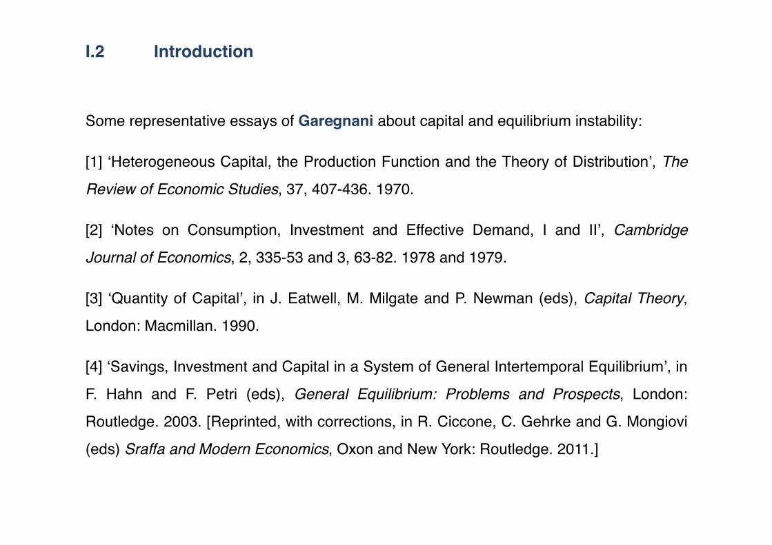
Let r* be an equilibrium – i.e. v(r*) = vs(r*) – following the standard arguments we say that
r* is locally (asymptotically) stable if the excess demand for capital and the interest rate
vary in opposite directions in a neighbourhood of r*.!
Local stability:!
€
dvdr r*
−dvs
drr*
< 0
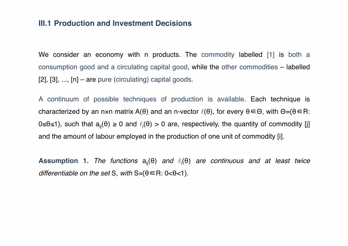
III.1 !Production and Investment Decisions !
We consider an economy with n products. The commodity labelled [1] is both a
consumption good and a circulating capital good, while the other commodities – labelled
[2], [3], ..., [n] – are pure (circulating) capital goods.!
A continuum of possible techniques of production is available. Each technique is
characterized by an n×n matrix A(θ) and an n-vector (θ), for every θ∈Θ, with Θ={θ∈R:
0≤θ≤1}, such that aij(θ) ≥ 0 and i(θ) > 0 are, respectively, the quantity of commodity [j]
and the amount of labour employed in the production of one unit of commodity [i].!
Assumption 1. The functions aij(θ) and i(θ) are continuous and at least twice
differentiable on the set S, with S={θ∈R: 0<θ<1}.!
III.2 !Production and Investment Decisions !
For each technique θ, there exist a scalar y(θ) and a (row) vector q(θ) that are
respectively the net product of commodity [1] per worker and the vector of activity levels
generating it. These can be obtained by solving the following equations:!
(2)!
(3)!
Assumption 2. No technique in Θ is dominated. That is, for every technique θ∈Θ, there
exists no other technique θʼ such that y(θʼ) > y(θ), q(θʼ)A(θʼ) ≤ q(θ)A(θ) and q(θʼ)(θʼ)
≤ q(θ)(θ).!
Assumption 3. The techniques in Θ are labelled in such a way that y(θʼʼ) > y(θʼ)
whenever θʼʼ > θʼ.!
€
y(θ) ⋅ e1 = q(θ) ⋅[I−A(θ)]
€
1= q(θ) ⋅ (θ)

III.3 !Production and Investment Decisions !
Let us assume commodity [1] as the numéraire and denote with p(θ,r) and w(θ,r)
respectively the price vector and the wage rate that make the unit cost vector equal to the
price vector with the technique θ and the interest rate r.!
The function w(θ,r) is known as the wage-interest function or curve for technique θ. !

III.4 !Production and Investment Decisions !
According to a well-known result, given an interest rate r (taken within a certain interval),
the technique θ° is optimal if and only if w(θ°,r) ≥ w(θ,r) for every θ ∈ Θ.!
Therefore, solving the following maximisation problem:!
(4)!
with r considered parametrically between 0 and a certain maximum, makes it possible to
express the optimal technique as a function of the rate of interest: θ° = θ(r).!€
maxθ
w(θ, r)
s.t. : θ ∈Θ
⎧ ⎨ ⎪
⎩ ⎪
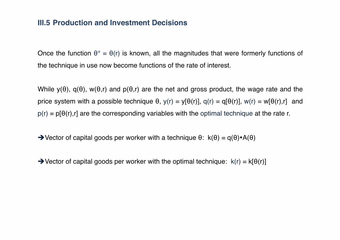
III.5 !Production and Investment Decisions !
Once the function θ° = θ(r) is known, all the magnitudes that were formerly functions of
the technique in use now become functions of the rate of interest. !
While y(θ), q(θ), w(θ,r) and p(θ,r) are the net and gross product, the wage rate and the
price system with a possible technique θ, y(r) = y[θ(r)], q(r) = q[θ(r)], w(r) = w[θ(r),r] and
p(r) = p[θ(r),r] are the corresponding variables with the optimal technique at the rate r.!
Vector of capital goods per worker with a technique θ: k(θ) = q(θ)A(θ)!
Vector of capital goods per worker with the optimal technique: k(r) = k[θ(r)]!
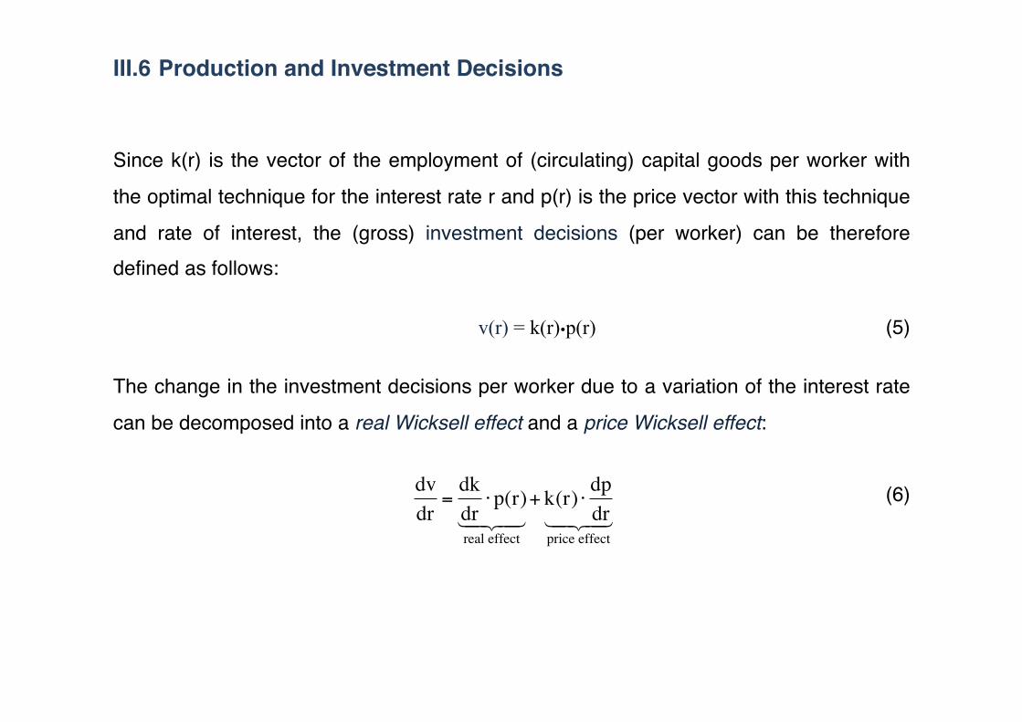
III.6 !Production and Investment Decisions !
Since k(r) is the vector of the employment of (circulating) capital goods per worker with
the optimal technique for the interest rate r and p(r) is the price vector with this technique
and rate of interest, the (gross) investment decisions (per worker) can be therefore defined as follows:!
v(r) = k(r)p(r) ! ! ! ! ! ! !(5)!
The change in the investment decisions per worker due to a variation of the interest rate
can be decomposed into a real Wicksell effect and a price Wicksell effect:!
(6)!
€
dvdr
=dkdr⋅p(r)
real effect
+ k(r) ⋅ dpdr
price effect

IV.1 !Reswitching and Real Wicksell Effect !
Reswitching can occur: it is possible for a technique to be optimal for two different levels of the interest rate but not for the levels between them.!
Reswitching implies a non-monotonic shape of the function y(r). This is particularly evident in our model, because there is a one-to-one correspondence between the technique in use and the amount of net product per worker (assumption 3).!
When r = 0, the optimal technique is θ = 1, i.e. the one with the greatest net product per worker. This implies that an increase in the rate of interest initially entails a decrease in the net product per worker.!
After the initial decreasing stretch, the pattern of the function y(r) becomes unpredictable. Since every technique can be brought back into use several times, the function y(r) can exhibit alternatively decreasing and increasing stretches.!

IV.2 !Reswitching and Real Wicksell Effect !
The sign of the variation in the net product per worker due to a rise in the rate of interest
is closely linked to that of the real Wicksell effect. This can be easily proved.!
Let us consider an interest rate r and denote by θ° the corresponding optimal technique,
while y° and k° are the net product and the vector of capital goods, both per worker, when
θ° is in use. Since technique θ° entails zero (extra)profits and is profit maximizing for r, p
(r) and w(r), then:!
(7)!
(8)!€
y°− r ⋅[k° ⋅ p(r)]− w(r) = 0
€
y°+dydθ
⎛
⎝ ⎜
⎞
⎠ ⎟ − r ⋅ k°+
dkdθ
⎛
⎝ ⎜
⎞
⎠ ⎟ ⋅ p(r)
⎡
⎣ ⎢
⎤
⎦ ⎥ − w(r) = 0

IV.3 !Reswitching and Real Wicksell Effect !
Therefore, substituting equation (7) in equation (8), we have:!
(9)!
Bearing in mind that y(r) = y[θ(r)] and k(r) = k[θ(r)], this clearly implies:!
(10)!
Therefore, for r > 0, the real Wicksell effect is negative if and only if dy/dr < 0. !
As a result, the reswitching of techniques entails a positive, i.e. anti-neo-classical, real
Wicksell effect.!
€
dydθ
− r ⋅ dkdθ
⋅ p(r) = 0
€
dy / dθdθ / dr
= r ⋅ dk / dθdθ / dr
⋅ p(r)

V.1 ! !Saving Decisions!
We consider an overlapping-generation model with identical individuals whose life lasts
for two periods. !
During the first period of life, each individual is a worker and inelastically supplies one
unit of labour. As a consequence, the individualʼs income in this period is equal to the
wage rate.!
In the second period, the individual becomes unable to work, and therefore her/his consumption depends on the part of the wage rate saved during the first period.!
Therefore, the wage rate is the only individual intertemporal income.!
V.2 ! !Saving Decisions!
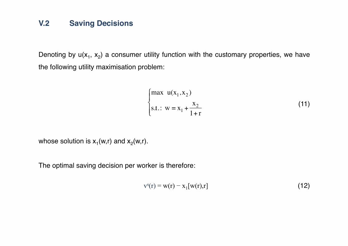
Denoting by u(x1, x2) a consumer utility function with the customary properties, we have
the following utility maximisation problem:!
(11)!
whose solution is x1(w,r) and x2(w,r).!
The optimal saving decision per worker is therefore:!
vs(r) = w(r) − x1[w(r),r] ! ! ! ! ! !(12)!
€
max u(x1,x2 )
s.t. : w = x1 +x2
1+ r
⎧
⎨ ⎪
⎩ ⎪

V.3 ! !Saving Decisions!
What can we say about the saving function vs(r) = w(r) – x1[w(r),r] ?!
Because of the usual substitution effect, an increase in the rate of interest (with a fixed w) should cause the consumption of the first period x1 to decrease with respect to the
consumption of the second period x2, but since there is also an income effect, x1 may
very well increase when the rate of interest increases. !
Moreover, the wage rate is inversely proportional to the rate of interest, and an increase in the latter will therefore decrease the income out of which savings are made. !
VI.1 !Equilibrium and Stability!
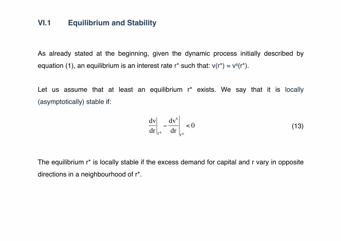
As already stated at the beginning, given the dynamic process initially described by
equation (1), an equilibrium is an interest rate r* such that: v(r*) = vs(r*).!
Let us assume that at least an equilibrium r* exists. We say that it is locally
(asymptotically) stable if:!
(13)!
The equilibrium r* is locally stable if the excess demand for capital and r vary in opposite
directions in a neighbourhood of r*. !€
dvdr r*
−dvs
drr*
< 0

VI.2 !Equilibrium and Stability!
The investment function derivative can be always decomposed into a real Wicksell effect
and a price Wicksell effect:!
(6bis)!
The two effects can be either positive or negative and the same or opposite in sign, so
that dv/dr can be negative even in a case with a positive real Wicksell effect (cf. Fratini
2010 for an example).!
€
dvdr r*
=dkdr r*
⋅p(r*)
real effect
+ k * ⋅dpdr r*
price effect

VI.3 !Equilibrium and Stability!
On the contrary, savings manifest themselves as a pure amount of value with no
specified physical shape, and can thus take every possible form. !
When an equilibrium is reached, however, savings are and must be converted into a
precise system of (real) assets: the equilibrium vector of capital goods k* = k(r*).
Therefore, in a small neighbourhood of r* only, we can therefore decompose the variation
of savings into an “asset value effect” and a “residuum” z: !
(14)!
€
dvs
drr*
= k *⋅dpdr r*
asset value effect
+ z
VI.4 !Equilibrium and Stability!
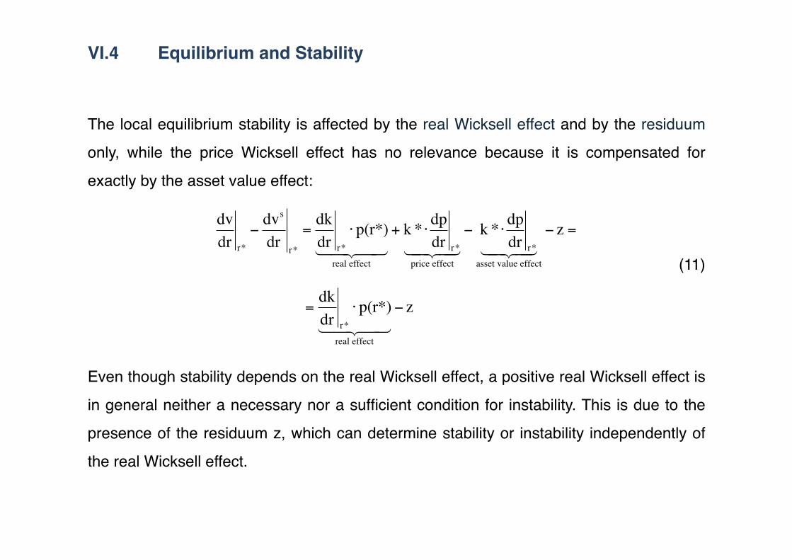
The local equilibrium stability is affected by the real Wicksell effect and by the residuum
only, while the price Wicksell effect has no relevance because it is compensated for
exactly by the asset value effect: !
(11)!
Even though stability depends on the real Wicksell effect, a positive real Wicksell effect is
in general neither a necessary nor a sufficient condition for instability. This is due to the
presence of the residuum z, which can determine stability or instability independently of
the real Wicksell effect. !
€
dvdr r*
−dvs
dr r*
=dkdr r*
⋅ p(r*)
real effect
+ k * ⋅ dpdr r*
price effect
− k * ⋅ dpdr r*
asset value effect
− z =
€
=dkdr r*
⋅ p(r*)
real effect
− z
VII.1 !Real Wicksell Effect and Stability!
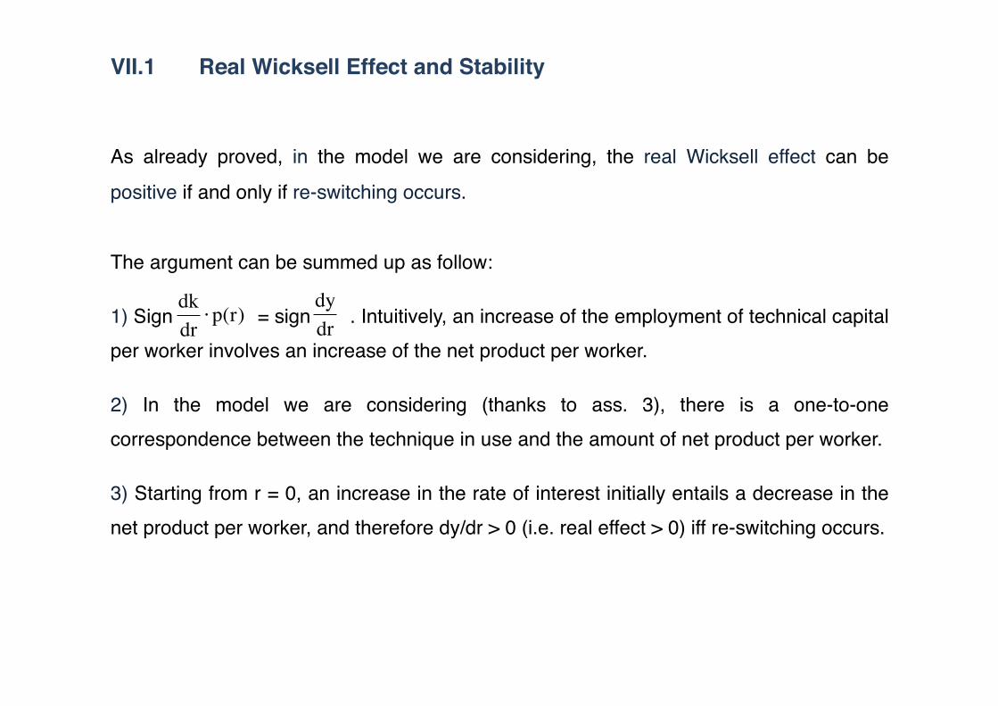
As already proved, in the model we are considering, the real Wicksell effect can be
positive if and only if re-switching occurs.!
The argument can be summed up as follow:!
1) Sign = sign . Intuitively, an increase of the employment of technical capital per worker involves an increase of the net product per worker.!
2) In the model we are considering (thanks to ass. 3), there is a one-to-one correspondence between the technique in use and the amount of net product per worker.!
3) Starting from r = 0, an increase in the rate of interest initially entails a decrease in the net product per worker, and therefore dy/dr > 0 (i.e. real effect > 0) iff re-switching occurs.!
€
dkdr⋅p(r)
€
dydr

VII.2 !Real Wicksell Effect and Stability!
A positive real Wicksell effect is in general neither a necessary nor a sufficient condition
for instability. The relevance of the real Wicksell effect for equilibrium stability can,
however, be studied by imposing some restrictions on the residuum.!
In particular, if we assume z ≥ 0 (which means that the change in savings due to an
increase in r is equal to or greater than the asset value effect) then the positive real
Wicksell effect becomes a necessary, but not sufficient, condition for instability.!
If we assume z = 0 (i.e. that savings vary exactly as much as the value of the equilibrium
vector of assets, at least in a small neighbourhood of r*), then the equilibrium can be
locally unstable if and only if the real Wicksell effect is positive.!

VII.3 !Real Wicksell Effect and Stability!
The stability of the equilibrium between investments and savings depends on the real
Wicksell effect and on the residuum. The shape of the investments or demand-for-capital
curve appears instead irrelevant for stability.!
In particular:!
- a monotonically decreasing investment function can coexists with a positive real
Wicksell effect (cf. Bidard 2010 and Fratini 2010);!
- a positive real Wicksell effect can be cause of instability;!- instability due to re-switching is possible even in the case of a monotonically decreasing
investment function.!
VIII.1 !Conclusions!
The possibility of an increasing demand for capital schedule, at least in a certain stretch,
which emerged as a result of the capital debate of the 1970s, has been viewed as a
possible cause of instability for the equilibrium on the capital market.!
This argument was mainly presented in terms of Wicksellʼs theory, where the
exogenously given supply of capital is misleading for two reasons:!
i) the property of stability seems to depend on the shape of the demand-for-capital
curve alone rather than the shape of the excess-demand curve, as is usually the case. !
ii) the value of any bundle of commodities cannot be consistently taken as given before
income distribution and relative prices are determined and, as a result, numerical
solutions of Wicksellʼs equations cannot be regarded as economically meaningful
equilibria.!

VIII.2 !Conclusions!
We have tried to put the possibility of instability arising from capital paradoxes on a
different basis.!
1) We used a particular device: we decomposed the change in savings due to a change
in the interest rate into an “asset value effect” and a residuum, and since the asset value
effect and the price Wicksell effect cancel out each other, we arrived at the conclusion
that the local stability of the equilibrium ultimately depends on the real Wicksell effect and
on the residuum.!
2) In cases where the residuum is well-behaved (or even negligible), instability is
therefore possible only if the real Wicksell effect is positive, as happens in the case of re-
switching. !

GRAZIE!
THANK YOU!
OBRIGADO!
감사합니다!
GRACIAS!
DANKE!