Embed Size (px)
Citation preview

Why the Laws of Physics Make Perfect Sense After All
THE WORLD ACCORDING TO QUANTUM MECHANICS
7592tp.indd 1 5/3/10 8:27:06 AM

This page intentionally left blankThis page intentionally left blank

N E W J E R S E Y • L O N D O N • S I N G A P O R E • BE IJ ING • S H A N G H A I • H O N G K O N G • TA I P E I • C H E N N A I
World Scientific
Ulrich Mohrhoff
Why the Laws of Physics Make Perfect Sense After All
THE WORLD ACCORDING TO QUANTUM MECHANICS
7592tp.indd 2 5/3/10 8:27:07 AM

British Library Cataloguing-in-Publication DataA catalogue record for this book is available from the British Library.
For photocopying of material in this volume, please pay a copying fee through the CopyrightClearance Center, Inc., 222 Rosewood Drive, Danvers, MA 01923, USA. In this case permission tophotocopy is not required from the publisher.
ISBN-13 978-981-4293-37-2ISBN-10 981-4293-37-7
All rights reserved. This book, or parts thereof, may not be reproduced in any form or by any means,electronic or mechanical, including photocopying, recording or any information storage and retrievalsystem now known or to be invented, without written permission from the Publisher.
Copyright © 2011 by World Scientific Publishing Co. Pte. Ltd.
Published by
World Scientific Publishing Co. Pte. Ltd.
5 Toh Tuck Link, Singapore 596224
USA office: 27 Warren Street, Suite 401-402, Hackensack, NJ 07601
UK office: 57 Shelton Street, Covent Garden, London WC2H 9HE
Printed in Singapore.
THE WORLD ACCORDING TO QUANTUM MECHANICSWhy the Laws of Physics Make Perfect Sense After All
Benjamin - The World According to Quan Mech.pmd 3/4/2011, 11:23 AM1

November 24, 2010 10:17 World Scientific Book - 9in x 6in main
Preface
While still in high school, I learned that the tides act as a brake on the
Earth’s rotation, gradually slowing it down, and that the angular momen-
tum lost by the rotating Earth is transferred to the Moon, causing it to
slowly spiral outwards, away from Earth. I still vividly remember my puz-
zlement. How, by what mechanism or process, did angular momentum get
transferred from Earth to the Moon? Just so Newton’s contemporaries
must have wondered at his theory of gravity. Newton’s response is well
known:
I have not been able to discover the cause of those properties ofgravity from phænomena, and I frame no hypotheses. . . . to usit is enough, that gravity does really exist, and act accordingto the laws which we have explained, and abundantly serves toaccount for all the motions of the celestial bodies, and of oursea. [Newton (1729)]
In Newton’s theory, gravitational effects were simultaneous with their
causes. The time-delay between causes and effects in classical electrody-
namics and in Einstein’s theory of gravity made it seem possible for a while
to explain “how Nature does it.” One only had to transmogrify the al-
gorithms that served to calculate the effects of given causes into physical
processes by which causes produce their effects. This is how the electro-
magnetic field—a calculational tool—came to be thought of as a physical
entity in its own right, which is locally acted upon by charges, which locally
acts on charges, and which mediates the action of charges on charges by
locally acting on itself.
Today this sleight of hand no longer works. While classical states
are algorithms that assign trivial probabilities—either 0 or 1—to measure-
ment outcomes (which is why they can be re-interpreted as collections of
v

November 24, 2010 10:17 World Scientific Book - 9in x 6in main
vi The World According to Quantum Mechanics
possessed properties and described without reference to “measurement”),
quantum states are algorithms that assign probabilities between 0 and 1
(which is why they cannot be so described). And while the classical laws
correlate measurement outcomes deterministically (which is why they can
be interpreted in causal terms and thus as descriptive of physical processes),
the quantum-mechanical laws correlate measurement outcomes probabilisti-
cally (which is why they cannot be so interpreted). In at least one respect,
therefore, physics is back to where it was in Newton’s time—and this with
a vengeance. According to Dennis Dieks, Professor of the Foundations and
Philosophy of the Natural Sciences at Utrecht University and Editor of
Studies in History and Philosophy of Modern Physics,
the outcome of foundational work in the last couple of decadeshas been that interpretations which try to accommodate classi-cal intuitions are impossible, on the grounds that theories thatincorporate such intuitions necessarily lead to empirical pre-dictions which are at variance with the quantum mechanicalpredictions. [Dieks (1996)]
But, seriously, how could anyone have hoped to get away for good with
passing off computational tools—mathematical symbols or equations—as
physical entities or processes? Was it the hubristic desire to feel “potentially
omniscient”—capable in principle of knowing the furniture of the universe
and the laws by which this is governed?
If quantum mechanics is the fundamental theoretical framework of
physics—and while there are a few doubters [e.g., Penrose (2005)], no-
body has the slightest idea what an alternative framework consistent with
the empirical data might look like—then the quantum formalism not only
defies reification but also cannot be explained in terms of a “more fun-
damental” framework. We sometimes speak loosely of a theory as being
more fundamental than another but, strictly speaking, “fundamental” has
no comparative. This is another reason why we cannot hope to explain
“how Nature does it.” What remains possible is to explain “why Nature
does it.” When efficient causation fails, teleological explanation remains
viable.
The question that will be centrally pursued in this book is: what does
it take to have stable objects that “occupy space” while being composed of
objects that do not “occupy space”?1 And part of the answer at which we
shall arrive is: quantum mechanics.1The existence of such objects is a well-established fact. According to the well-tested
theories of particle physics, which are collectively known as the Standard Model, theobjects that do not “occupy space” are the quarks and the leptons.

November 24, 2010 10:17 World Scientific Book - 9in x 6in main
Preface vii
As said, quantum states are algorithms that assign probabilities between
0 and 1. Think of them as computing machines: you enter (i) the actual
outcome(s) and time(s) of one or several measurements, as well as (ii) the
possible outcomes and the time of a subsequent measurement—and out pop
the probabilities of these outcomes. Even though the time dependence of a
quantum state is thus clearly a dependence on the times of measurements, it
is generally interpreted—even in textbooks that strive to remain metaphys-
ically uncommitted—as a dependence on “time itself,” and thus as the time
dependence of something that exists at every moment of time and evolves
from earlier to later times. Hence the mother of all quantum-theoretical
pseudo-questions: why does a quantum state have (or appear to have) two
modes of evolution—continuous and predictable between measurements,
discontinuous and unpredictable whenever a measurement is made?
The problem posed by the central role played by measurements in stan-
dard axiomatizations of quantum mechanics is known as the “measurement
problem.” Although the actual number of a quantum state’s modes of evo-
lution is zero, most attempts to solve the measurement problem aim at
reducing the number of modes from two to one. As an anonymous referee
once put it to me, “to solve this problem means to design an interpretation
in which measurement processes are not different in principle from ordinary
physical interactions.” The way I see it, to solve the measurement problem
means, on the contrary, to design an interpretation in which the central role
played by measurements is understood, rather than swept under the rug.
An approach that rejects the very notion of quantum state evolution
runs the risk of being dismissed as an ontologically sterile instrumental-
ism. Yet it is this notion, more than any other, that blocks our view of
the ontological implications of quantum mechanics. One of these impli-
cations is that the spatiotemporal differentiation of the physical world is
incomplete; it does not “go all the way down.” The notion that quantum
states evolve, on the other hand, implies that it does “go all the way down.”
This is not simply a case of one word against another, for the incomplete
spatiotemporal differentiation of the physical world follows from the man-
ner in which quantum mechanics assigns probabilities, which is testable,
whereas the complete spatiotemporal differentiation of the physical world
follows from an assumption about what is the case between measurements ,
and such an assumption is “not even wrong” in Wolfgang Pauli’s famous
phrase, inasmuch as it is neither verifiable nor falsifiable.
Understanding the central role played by measurements calls for a clear
distinction between what measures and what is measured, and this in turn

November 24, 2010 10:17 World Scientific Book - 9in x 6in main
viii The World According to Quantum Mechanics
calls for a precise definition of the frequently misused and much maligned
word “macroscopic.” Since it is the incomplete differentiation of the phys-
ical world that makes such a definition possible, the central role played
by measurements cannot be understood without dispelling the notion that
quantum states evolve.
For at least twenty-five centuries, theorists—from metaphysicians to
natural philosophers to physicists and philosophers of science—have tried
to model reality from the bottom up, starting with an ultimate multiplicity
and using concepts of composition and interaction as their basic explana-
tory tools. If the spatiotemporal differentiation of the physical world is
incomplete, then the attempt to understand the world from the bottom
up—whether on the basis of an intrinsically and completely differentiated
space or spacetime, out of locally instantiated physical properties, or by ag-
gregation, out of a multitude of individual substances—is doomed to failure.
What quantum mechanics is trying to tell us is that reality is structured
from the top down.
Having explained why interpretations that try to accommodate classical
intuitions are impossible, Dieks goes on to say:
However, this is a negative result that only provides us with astarting-point for what really has to be done: something con-ceptually new has to be found, different from what we are famil-iar with. It is clear that this constructive task is a particularlydifficult one, in which huge barriers (partly of a psychologicalnature) have to be overcome. [Dieks (1996)]
Something conceptually new has been found, and is presented in this book.
To make the presentation reasonably self-contained, and to make those
already familiar with the subject aware of metaphysical prejudices they
may have acquired in the process of studying it, the format is that of a
textbook. To make the presentation accessible to a wider audience—not
only students of physics and their teachers—the mathematical tools used
are introduced along the way, to the point that the theoretical concepts used
can be adequately grasped. In doing so, I tried to adhere to a principle that
has been dubbed “Einstein’s razor”: everything should be made as simple
as possible, but no simpler.
This textbook is based on a philosophically oriented course of con-
temporary physics I have been teaching for the last ten years at the Sri
Aurobindo International Centre of Education (SAICE) in Puducherry (for-
merly Pondicherry), India. This non-compulsory course is open to higher

November 24, 2010 10:17 World Scientific Book - 9in x 6in main
Preface ix
secondary (standards 10–12) and undergraduate students, including stu-
dents with negligible prior exposure to classical physics.2
The text is divided into three parts. After a short introduction to prob-
ability, Part 1 (“Overview”) follows two routes that lead to the Schrodinger
equation—the historical route and Feynman’s path-integral approach. On
the first route we stop once to gather the needed mathematical tools, and
on the second route we stop once for an introduction to the special theory
of relativity.
The first chapter of Part 2 (“A Closer Look”) derives the mathematical
formalism of quantum mechanics from the existence of “ordinary” objects—
stable objects that “occupy space” while being composed of objects that
do not “occupy space.” The next two chapters are concerned with what
happens if the objective fuzziness that “fluffs out” matter is ignored. (What
happens is that the quantum-mechanical correlation laws degenerate into
the dynamical laws of classical physics.) The remainder of Part 2 covers
a number of conceptually challenging experiments and theoretical results,
along with more conventional topics.
Part 3 (“Making Sense”) deals with the ontological implications of the
formalism of quantum mechanics. The penultimate chapter argues that
quantum mechanics—whose validity is required for the existence of “ordi-
nary” objects—in turn requires for its consistency the validity of both the
Standard Model and the general theory of relativity, at least as effective
theories. The final chapter hazards an answer to the question of why stable
objects that “occupy space” are composed of objects that do not “occupy
space.” It is followed by an appendix containing solutions or hints for some
of the problems provided in the text.
2I consider this a plus. In the first section of his brilliant Caltech lectures [Feynmanet al. (1963)], Richard Feynman raised a question of concern to every physics teacher:“Should we teach the correct but unfamiliar law with its strange and difficult conceptualideas . . . ? Or should we first teach the simple . . . law, which is only approximate, butdoes not involve such difficult ideas? The first is more exciting, more wonderful, andmore fun, but the second is easier to get at first, and is a first step to a real understandingof the second idea.” With all due respect to one of the greatest physicists of the 20thCentury, I cannot bring myself to agree. How can the second approach be a step to areal understanding of the correct law if “philosophically we are completely wrong withthe approximate law,” as Feynman himself emphasized in the immediately precedingparagraph? To first teach laws that are completely wrong philosophically cannot butimpart a conceptual framework that eventually stands in the way of understanding thecorrect laws. The damage done by imparting philosophically wrong ideas to youngstudents is not easily repaired.

November 24, 2010 10:17 World Scientific Book - 9in x 6in main
x The World According to Quantum Mechanics
I wish to thank the SAICE for the opportunity to teach this exper-
imental course in “quantum philosophy” and my students—the “guinea
pigs”—for their valuable feedback.
Ulrich Mohrhoff
August 15, 2010

November 24, 2010 10:50 World Scientific Book - 9in x 6in main
Contents
Preface v
Overview 1
1. Probability: Basic concepts and theorems 3
1.1 The principle of indifference . . . . . . . . . . . . . . . . . 3
1.2 Subjective probabilities versus objective probabilities . . . 4
1.3 Relative frequencies . . . . . . . . . . . . . . . . . . . . . 4
1.4 Adding and multiplying probabilities . . . . . . . . . . . . 5
1.5 Conditional probabilities and correlations . . . . . . . . . 7
1.6 Expectation value and standard deviation . . . . . . . . . 8
2. A (very) brief history of the “old” theory 9
2.1 Planck . . . . . . . . . . . . . . . . . . . . . . . . . . . . . 9
2.2 Rutherford . . . . . . . . . . . . . . . . . . . . . . . . . . 9
2.3 Bohr . . . . . . . . . . . . . . . . . . . . . . . . . . . . . . 10
2.4 de Broglie . . . . . . . . . . . . . . . . . . . . . . . . . . . 12
3. Mathematical interlude 15
3.1 Vectors . . . . . . . . . . . . . . . . . . . . . . . . . . . . 15
3.2 Definite integrals . . . . . . . . . . . . . . . . . . . . . . . 17
3.3 Derivatives . . . . . . . . . . . . . . . . . . . . . . . . . . 19
3.4 Taylor series . . . . . . . . . . . . . . . . . . . . . . . . . . 23
3.5 Exponential function . . . . . . . . . . . . . . . . . . . . . 23
3.6 Sine and cosine . . . . . . . . . . . . . . . . . . . . . . . . 24
3.7 Integrals . . . . . . . . . . . . . . . . . . . . . . . . . . . . 25
xi
November 24, 2010 10:50 World Scientific Book - 9in x 6in main
xii The World According to Quantum Mechanics
3.8 Complex numbers . . . . . . . . . . . . . . . . . . . . . . 27
4. A (very) brief history of the “new” theory 31
4.1 Schrodinger . . . . . . . . . . . . . . . . . . . . . . . . . . 31
4.2 Born . . . . . . . . . . . . . . . . . . . . . . . . . . . . . . 33
4.3 Heisenberg and “uncertainty” . . . . . . . . . . . . . . . . 35
4.4 Why energy is quantized . . . . . . . . . . . . . . . . . . . 38
5. The Feynman route to Schrodinger (stage 1) 41
5.1 The rules of the game . . . . . . . . . . . . . . . . . . . . 41
5.2 Two slits . . . . . . . . . . . . . . . . . . . . . . . . . . . 41
5.2.1 Why product? . . . . . . . . . . . . . . . . . . . . 42
5.2.2 Why inverse proportional to BA? . . . . . . . . . 43
5.2.3 Why proportional to BA? . . . . . . . . . . . . . 43
5.3 Interference . . . . . . . . . . . . . . . . . . . . . . . . . . 44
5.3.1 Limits to the visibility of interference fringes . . . 45
5.4 The propagator as a path integral . . . . . . . . . . . . . 47
5.5 The time-dependent propagator . . . . . . . . . . . . . . . 48
5.6 A free particle . . . . . . . . . . . . . . . . . . . . . . . . . 50
5.7 A free and stable particle . . . . . . . . . . . . . . . . . . 50
6. Special relativity in a nutshell 53
6.1 The principle of relativity . . . . . . . . . . . . . . . . . . 53
6.2 Lorentz transformations: General form . . . . . . . . . . . 54
6.3 Composition of velocities . . . . . . . . . . . . . . . . . . 58
6.4 The case against positive K . . . . . . . . . . . . . . . . . 59
6.5 An invariant speed . . . . . . . . . . . . . . . . . . . . . . 61
6.6 Proper time . . . . . . . . . . . . . . . . . . . . . . . . . . 62
6.7 The meaning of mass . . . . . . . . . . . . . . . . . . . . . 63
6.8 The case against K = 0 . . . . . . . . . . . . . . . . . . . 64
6.9 Lorentz transformations: Some implications . . . . . . . . 65
6.10 4-vectors . . . . . . . . . . . . . . . . . . . . . . . . . . . . 68
7. The Feynman route to Schrodinger (stage 2) 69
7.1 Action . . . . . . . . . . . . . . . . . . . . . . . . . . . . . 69
7.2 How to influence a stable particle? . . . . . . . . . . . . . 70
7.3 Enter the wave function . . . . . . . . . . . . . . . . . . . 71
7.4 The Schrodinger equation . . . . . . . . . . . . . . . . . . 71

November 24, 2010 10:50 World Scientific Book - 9in x 6in main
Contents xiii
A Closer Look 75
8. Why quantum mechanics? 77
8.1 The classical probability calculus . . . . . . . . . . . . . . 77
8.2 Why nontrivial probabilities? . . . . . . . . . . . . . . . . 79
8.3 Upgrading from classical to quantum . . . . . . . . . . . . 80
8.4 Vector spaces . . . . . . . . . . . . . . . . . . . . . . . . . 80
8.4.1 Why complex numbers? . . . . . . . . . . . . . . . 82
8.4.2 Subspaces and projectors . . . . . . . . . . . . . . 82
8.4.3 Commuting and non-commuting projectors . . . . 84
8.5 Compatible and incompatible elementary tests . . . . . . 86
8.6 Noncontextuality . . . . . . . . . . . . . . . . . . . . . . . 88
8.7 The core postulates . . . . . . . . . . . . . . . . . . . . . . 90
8.8 The trace rule . . . . . . . . . . . . . . . . . . . . . . . . . 90
8.9 Self-adjoint operators and the spectral theorem . . . . . . 92
8.10 Pure states and mixed states . . . . . . . . . . . . . . . . 93
8.11 How probabilities depend on measurement outcomes . . . 94
8.12 How probabilities depend on the times of measurements . 95
8.12.1 Unitary operators . . . . . . . . . . . . . . . . . . 96
8.12.2 Continuous variables . . . . . . . . . . . . . . . . 99
8.13 The rules of the game derived at last . . . . . . . . . . . . 100
9. The classical forces: Effects 101
9.1 The principle of “least” action . . . . . . . . . . . . . . . 101
9.2 Geodesic equations for flat spacetime . . . . . . . . . . . . 104
9.3 Energy and momentum . . . . . . . . . . . . . . . . . . . 105
9.4 Vector analysis: Some basic concepts . . . . . . . . . . . . 107
9.4.1 Curl and Stokes’s theorem . . . . . . . . . . . . . 108
9.4.2 Divergence and Gauss’s theorem . . . . . . . . . . 110
9.5 The Lorentz force . . . . . . . . . . . . . . . . . . . . . . . 111
9.5.1 How the electromagnetic field bends geodesics . . 113
9.6 Curved spacetime . . . . . . . . . . . . . . . . . . . . . . . 115
9.6.1 Geodesic equations for curved spacetime . . . . . 116
9.6.2 Raising and lowering indices . . . . . . . . . . . . 116
9.6.3 Curvature . . . . . . . . . . . . . . . . . . . . . . 117
9.6.4 Parallel transport . . . . . . . . . . . . . . . . . . 118
9.7 Gravity . . . . . . . . . . . . . . . . . . . . . . . . . . . . 120
10. The classical forces: Causes 123

November 24, 2010 10:50 World Scientific Book - 9in x 6in main
xiv The World According to Quantum Mechanics
10.1 Gauge invariance . . . . . . . . . . . . . . . . . . . . . . . 123
10.2 Fuzzy potentials . . . . . . . . . . . . . . . . . . . . . . . 124
10.2.1 Lagrange function and Lagrange density . . . . . 125
10.3 Maxwell’s equations . . . . . . . . . . . . . . . . . . . . . 126
10.3.1 Charge conservation . . . . . . . . . . . . . . . . . 128
10.4 A fuzzy metric . . . . . . . . . . . . . . . . . . . . . . . . 129
10.4.1 Meaning of the curvature tensor . . . . . . . . . . 130
10.4.2 Cosmological constant . . . . . . . . . . . . . . . . 131
10.5 Einstein’s equation . . . . . . . . . . . . . . . . . . . . . . 131
10.5.1 The energy–momentum tensor . . . . . . . . . . . 132
10.6 Aharonov–Bohm effect . . . . . . . . . . . . . . . . . . . . 132
10.7 Fact and fiction in the world of classical physics . . . . . . 134
10.7.1 Retardation of effects and the invariant speed . . 136
11. Quantum mechanics resumed 139
11.1 The experiment of Elitzur and Vaidman . . . . . . . . . . 139
11.2 Observables . . . . . . . . . . . . . . . . . . . . . . . . . . 141
11.3 The continuous case . . . . . . . . . . . . . . . . . . . . . 142
11.4 Commutators . . . . . . . . . . . . . . . . . . . . . . . . . 143
11.5 The Heisenberg equation . . . . . . . . . . . . . . . . . . . 144
11.6 Operators for energy and momentum . . . . . . . . . . . . 144
11.7 Angular momentum . . . . . . . . . . . . . . . . . . . . . 145
11.8 The hydrogen atom in brief . . . . . . . . . . . . . . . . . 147
12. Spin 153
12.1 Spin 1/2 . . . . . . . . . . . . . . . . . . . . . . . . . . . . 153
12.1.1 Other bases . . . . . . . . . . . . . . . . . . . . . 155
12.1.2 Rotations as 2× 2 matrices . . . . . . . . . . . . . 156
12.1.3 Pauli spin matrices . . . . . . . . . . . . . . . . . 159
12.2 A Stern–Gerlach relay . . . . . . . . . . . . . . . . . . . . 160
12.3 Why spin? . . . . . . . . . . . . . . . . . . . . . . . . . . . 162
12.4 Beyond hydrogen . . . . . . . . . . . . . . . . . . . . . . . 163
12.5 Spin precession . . . . . . . . . . . . . . . . . . . . . . . . 166
12.6 The quantum Zeno effect . . . . . . . . . . . . . . . . . . 167
13. Composite systems 169
13.1 Bell’s theorem: The simplest version . . . . . . . . . . . . 169
13.2 “Entangled” spins . . . . . . . . . . . . . . . . . . . . . . 171

November 24, 2010 10:50 World Scientific Book - 9in x 6in main
Contents xv
13.2.1 The singlet state . . . . . . . . . . . . . . . . . . . 172
13.3 Reduced density operator . . . . . . . . . . . . . . . . . . 173
13.4 Contextuality . . . . . . . . . . . . . . . . . . . . . . . . . 174
13.5 The experiment of Greenberger, Horne, and Zeilinger . . . 177
13.5.1 A game . . . . . . . . . . . . . . . . . . . . . . . . 177
13.5.2 A fail-safe strategy . . . . . . . . . . . . . . . . . 178
13.6 Uses and abuses of counterfactual reasoning . . . . . . . . 179
13.7 The experiment of Englert, Scully, and Walther . . . . . . 184
13.7.1 The experiment with shutters closed . . . . . . . . 185
13.7.2 The experiment with shutters opened . . . . . . . 186
13.7.3 Influencing the past . . . . . . . . . . . . . . . . . 187
13.8 Time-symmetric probability assignments . . . . . . . . . . 190
13.8.1 A three-hole experiment . . . . . . . . . . . . . . 192
14. Quantum statistics 195
14.1 Scattering billiard balls . . . . . . . . . . . . . . . . . . . 195
14.2 Scattering particles . . . . . . . . . . . . . . . . . . . . . . 195
14.2.1 Indistinguishable macroscopic objects? . . . . . . 197
14.3 Symmetrization . . . . . . . . . . . . . . . . . . . . . . . . 198
14.4 Bosons are gregarious . . . . . . . . . . . . . . . . . . . . 198
14.5 Fermions are solitary . . . . . . . . . . . . . . . . . . . . . 199
14.6 Quantum coins and quantum dice . . . . . . . . . . . . . 200
14.7 Measuring Sirius . . . . . . . . . . . . . . . . . . . . . . . 201
15. Relativistic particles 205
15.1 The Klein–Gordon equation . . . . . . . . . . . . . . . . . 205
15.2 Antiparticles . . . . . . . . . . . . . . . . . . . . . . . . . 206
15.3 The Dirac equation . . . . . . . . . . . . . . . . . . . . . . 207
15.4 The Euler–Lagrange equation . . . . . . . . . . . . . . . . 208
15.5 Noether’s theorem . . . . . . . . . . . . . . . . . . . . . . 210
15.6 Scattering amplitudes . . . . . . . . . . . . . . . . . . . . 211
15.7 QED . . . . . . . . . . . . . . . . . . . . . . . . . . . . . . 212
15.8 A few words about renormalization . . . . . . . . . . . . . 212
15.8.1 . . . and about Feynman diagrams . . . . . . . . . . 215
15.9 Beyond QED . . . . . . . . . . . . . . . . . . . . . . . . . 216
15.9.1 QED revisited . . . . . . . . . . . . . . . . . . . . 217
15.9.2 Groups . . . . . . . . . . . . . . . . . . . . . . . . 217
15.9.3 Generalizing QED . . . . . . . . . . . . . . . . . . 218

November 24, 2010 10:50 World Scientific Book - 9in x 6in main
xvi The World According to Quantum Mechanics
15.9.4 QCD . . . . . . . . . . . . . . . . . . . . . . . . . 219
15.9.5 Electroweak interactions . . . . . . . . . . . . . . 220
15.9.6 Higgs mechanism . . . . . . . . . . . . . . . . . . 221
Making Sense 223
16. Pitfalls 225
16.1 Standard axioms: A critique . . . . . . . . . . . . . . . . . 225
16.2 The principle of evolution . . . . . . . . . . . . . . . . . . 227
16.3 The eigenstate–eigenvalue link . . . . . . . . . . . . . . . 229
17. Interpretational strategy 231
18. Spatial aspects of the quantum world 233
18.1 The two-slit experiment revisited . . . . . . . . . . . . . . 233
18.1.1 Bohmian mechanics . . . . . . . . . . . . . . . . . 234
18.1.2 The meaning of “both” . . . . . . . . . . . . . . . 235
18.2 The importance of unperformed measurements . . . . . . 235
18.3 Spatial distinctions: Relative and contingent . . . . . . . 237
18.4 The importance of detectors . . . . . . . . . . . . . . . . . 237
18.4.1 A possible objection . . . . . . . . . . . . . . . . . 238
18.5 Spatiotemporal distinctions: Not all the way down . . . . 238
18.6 The shapes of things . . . . . . . . . . . . . . . . . . . . . 240
18.7 Space . . . . . . . . . . . . . . . . . . . . . . . . . . . . . 240
19. The macroworld 243
20. Questions of substance 247
20.1 Particles . . . . . . . . . . . . . . . . . . . . . . . . . . . . 247
20.2 Scattering experiment revisited . . . . . . . . . . . . . . . 247
20.3 How many constituents? . . . . . . . . . . . . . . . . . . . 248
20.4 An ancient conundrum . . . . . . . . . . . . . . . . . . . . 249
20.5 A fundamental particle by itself . . . . . . . . . . . . . . . 250
21. Manifestation 251
21.1 “Creation” in a nutshell . . . . . . . . . . . . . . . . . . . 251
21.2 The coming into being of form . . . . . . . . . . . . . . . 251

November 24, 2010 10:50 World Scientific Book - 9in x 6in main
Contents xvii
21.3 Bottom-up or top-down? . . . . . . . . . . . . . . . . . . . 252
21.4 Whence the quantum-mechanical correlation laws? . . . . 253
21.5 How are “spooky actions at a distance” possible? . . . . . 254
22. Why the laws of physics are just so 257
22.1 The stability of matter . . . . . . . . . . . . . . . . . . . . 257
22.2 Why quantum mechanics (summary) . . . . . . . . . . . . 258
22.3 Why special relativity (summary) . . . . . . . . . . . . . . 260
22.4 Why quantum mechanics (summary continued) . . . . . . 260
22.5 The classical or long-range forces . . . . . . . . . . . . . . 261
22.6 The nuclear or short-range forces . . . . . . . . . . . . . . 262
22.7 Fine tuning . . . . . . . . . . . . . . . . . . . . . . . . . . 264
23. Quanta and Vedanta 267
23.1 The central affirmation . . . . . . . . . . . . . . . . . . . . 268
23.2 The poises of creative consciousness . . . . . . . . . . . . 269
Appendix A. Solutions to selected problems 271
Bibliography 277
Index 283

This page intentionally left blankThis page intentionally left blank

November 24, 2010 10:17 World Scientific Book - 9in x 6in main
PART 1
Overview
1

November 24, 2010 10:17 World Scientific Book - 9in x 6in main
2
This page intentionally left blankThis page intentionally left blank

December 23, 2010 9:50 World Scientific Book - 9in x 6in main
Chapter 1
Probability:Basic concepts and theorems
The mathematical formalism of quantum mechanics is a probability cal-
culus. The probability algorithms it places at our disposal—state vectors,
wave functions, density matrices, statistical operators—all serve the same
purpose, which is to calculate the probabilities of measurement outcomes.
That’s reason enough to begin by putting together what we already know
and what we need to know about probabilities.
1.1 The principle of indifference
Probability is a measure of likelihood ranging from 0 to 1. If an event has a
probability equal to 1, it is certain that it will happen; if it has a probability
equal to 0, it is certain that it will not happen; and if it has a probability
equal to 1/2, then it is as likely as not that it will happen.
Tossing a fair coin yields heads with probability 1/2. Casting a fair
die yields any given natural number between 1 and 6 with probability 1/6.
These are just two examples of the principle of indifference, which states:
If there are n mutually exclusive and jointly exhaustive possibilities (or
possible events), and if we have no reason to consider any one of them more
likely than any other, then each possibility should be assigned a probability
equal to 1/n.
Saying that events aremutually exclusive is the same as saying that at most
one of them happens. Saying that events are jointly exhaustive is the same
as saying that at least one of them happens.
3

December 23, 2010 9:50 World Scientific Book - 9in x 6in main
4 The World According to Quantum Mechanics
1.2 Subjective probabilities versus objective probabilities
There are two kinds of situations in which we may have no reason to consider
one possibility more likely than another. In situations of the first kind, there
are objective matters of fact that would make it certain, if we knew them,
that a particular event will happen, but we don’t know any of the relevant
matters of fact. The probabilities we assign in this case, or whenever we
know some but not all relevant facts, are in an obvious sense subjective.
They are ignorance probabilities. They have everything to do with our
(lack of) knowledge of relevant facts, but nothing with the existence of
relevant facts. Therefore they are also known as epistemic probabilities.
In situations of the second kind, there are no objective matters of fact
that would make it certain that a particular event will happen. There
may not even be objective matters of fact that would make it more likely
that one event will occur rather than another. There isn’t any relevant
fact that we are ignorant of. The probabilities we assign in this case are
neither subjective nor epistemic. They deserve to be considered objective.
Quantum-mechanical probabilities are essentially of this kind.
Until the advent of quantum mechanics, all probabilities were thought
to be subjective. This had two unfortunate consequences. The first is that
probabilities came to be thought of as something intrinsically subjective.
The second is that something that was not a probability at all—namely, a
relative frequency—came to be called an “objective probability.”
1.3 Relative frequencies
Relative frequencies are useful in that they allow us to measure the like-
lihood of possible events, at least approximately, provided that trials can
be repeated under conditions that are identical in all relevant respects. We
obviously cannot measure the likelihood of heads by tossing a single coin.
But since we can toss a coin any number of times, we can count the number
NH of heads and the number NT of tails obtained in N tosses and calculate
the fraction fHN = NH/N of heads and the fraction fT
N = NT /N of tails.
And we can expect the difference |NH−NT | to increase significantly slower
than the sum N = NH +NT , so that
limN→∞
|NH −NT |NH +NT
= limN→∞
|fHN − fT
N | = 0 . (1.1)

November 24, 2010 10:17 World Scientific Book - 9in x 6in main
Probability: Basic concepts and theorems 5
In other words, we can expect the relative frequencies fHN and fT
N to tend
to the probabilities pH of heads and pT of tails, respectively:
pH = limN→∞
NH
N, pT = lim
N→∞
NT
N. (1.2)
1.4 Adding and multiplying probabilities
Suppose you roll a (six-sided) die. And suppose you win if you throw either
a 1 or a 6 (no matter which). Since there are six equiprobable outcomes,
two of which cause you to win, your chances of winning are 2/6. In this
example it is appropriate to add probabilities:
p(1 ∨ 6) = p(1) + p(6) =1
6+
1
6=
1
3. (1.3)
The symbol ∨ means “or.” The general rule is this:
Sum rule. Let W be a set of w mutually exclusive and jointly exhaustive
events (for instance, the possible outcomes of a measurement), and let Ube a subset of W containing a smaller number u of events: U ⊂ W , u < w.
The probability p(U) that one of the events e1, . . . , eu in U takes place (no
matter which) is the sum p1 + · · · + pu of the respective probabilities of
these events.
One nice thing about relative frequencies is that they make a rule such as
this virtually self-evident. To demonstrate this, let N be the total number
of trials—think coin tosses or measurements. Let Nk be the total number
of trials with outcome ek, and let N(U) be the total number of trials with
an outcome in U . As N tends to infinity, Nk/N tends to pk and N(U)/Ntends to p(U). But
N(U)
N=N1 + · · ·+Nu
N=N1
N+ · · ·+ Nu
N, (1.4)
and in the limit N →∞ this becomes
p(U) = p1 + · · ·+ pu . (1.5)
Suppose now that you roll two dice. And suppose that you win if your total
equals 12. Since there are now 6 × 6 equiprobable outcomes, only one of
which causes you to win, your chances of winning are 1/(6 × 6). In this
example it is appropriate to multiply probabilities:
p(6 ∧ 6) = p(6)× p(6) =1
6× 1
6=
1
36. (1.6)
December 23, 2010 9:50 World Scientific Book - 9in x 6in main
6 The World According to Quantum Mechanics
The symbol ∧ means “and.” Here is the general rule:
Product rule. The joint probability p(e1∧· · ·∧ev) of v independent eventse1, . . . , ev (that is, the probability with which all of them happen) is the
product of the probabilities p(e1), . . . , p(ev) of the individual events.
It must be stressed that the product rule only applies to independent events.
Saying that two events a, b are independent is the same as saying that the
probability of a is independent of whether or not b happens, and vice versa.
As an illustration of the product rule for two independent events, let
a1, . . . , aJ be mutually exclusive and jointly exhaustive events (think of the
possible outcomes of a measurement of a variable A), and let pa1 , . . . , paJ
be the corresponding probabilities. Let b1, . . . , bK be a second such set
of events with corresponding probabilities pb1, . . . , pbK . Now draw a 1 × 1
square with coordinates x, y ranging from 0 to 1. Partition it horizontally
into J strips of respective width paj . Partition it vertically into K strips
of respective width pbk. You now have a square partitioned into J × K
rectangles with respective areas paj × pbk. Since a joint measurement of A
and B is equivalent to throwing a dart in such a way that it hits a random
position (x, y) within the square, the joint probability p(aj ∧ bk) equals thecorresponding area.
Problem 1.1. We have seen that the probability of obtaining a total of 12
when rolling a pair of dice is 1/36. What is the probability of obtaining a
total of (a) 11, (b) 10, (c) 9?
Problem 1.2. (∗)1 In 1999, Sally Clark was convicted of murdering her
first two babies, which died in their sleep of sudden infant death syndrome.
She was sent to prison to serve two life sentences for murder, essentially on
the testimony of an “expert” who told the jury it was too improbable that two
children in one family would die of this rare syndrome, which has a proba-
bility of 1/8,500. After over three years in prison, and five years of fighting
in the legal system, Sally was cleared by a Court of Appeal, and another
two and a half years later, the “expert” pediatrician Sir Roy Meadow was
found guilty of serious professional misconduct. Amazingly, during the trial
nobody raise the objection that an expert pediatrician was not likely to be an
expert statistician. Meadow had argued that the probability of two sudden
infant deaths in the same family was (1/8, 500)×(1/8, 500) = 1/72, 250, 000.
Explain why he was so terribly wrong.
1A star indicates that a solution or a hint is provided in Appendix A.

November 24, 2010 10:17 World Scientific Book - 9in x 6in main
Probability: Basic concepts and theorems 7
1.5 Conditional probabilities and correlations
If the events aj and bk are not independent, we must distinguish between
marginal probabilities , which are assigned to the possible outcomes of ei-
ther measurement without taking account of the outcome of the other mea-
surement, and conditional probabilities , which are assigned to the possible
outcomes of either measurement depending on the outcome of the other
measurement. If aj and bk are not independent, their joint probability is
p(aj ∧ bk) = p(bk|aj) p(aj) = p(aj |bk) p(bk) , (1.7)
where p(aj) and p(bk) are marginal probabilities, while p(bk|aj) is the prob-
ability of bk conditional on the outcome aj and p(aj |bk) is the probability
of aj conditional on the outcome bk. This gives us the useful relation
p(b|a) =p(a ∧ b)p(a)
. (1.8)
Another useful rule is
p(a) = p(a|b) p(b) + p(a|b) p(b) , (1.9)
where b and b are two mutually exclusive and jointly exhaustive events.
(To obtain b is to obtain any outcome other than b.) The validity of this
rule is again readily established with the help of relative frequencies. We
obviously have that
N(a)
N=N(a ∧ b)
N+N(a ∧ b)
N=N(a ∧ b)N(b)
N(b)
N+N(a ∧ b)N(b)
N(b)
N, (1.10)
where N is the number of joint measurements of two variables, one with
the possible outcome a and one with the possible outcome b. In the limit
N → ∞, N(a)/N (the left-hand side of Eq. 1.10) tends to the marginal
probability p(a), while the right-hand side of this equation tends to the
right-hand side of Eq. (1.9), as will be obvious from a glance at Eq. (1.8).
An important concept is that of (probabilistic) correlation. Two events
a, b are correlated just in case that p(a|b) 6= p(a|b). Specifically, a and b are
positively correlated if p(a|b) > p(a|b), and they are negatively correlated if
p(a|b) < p(a|b). Saying that a and b are independent is thus the same as
saying that they are uncorrelated, in which case p(a|b) = p(a|b) = p(a).
Problem 1.3. (∗) Let’s Make a Deal was a famous game show hosted by
Monty Hall. In it a player was to open one of three doors. Behind one door
there was the Grand Prize (for example, a car). Behind the other doors

November 24, 2010 10:17 World Scientific Book - 9in x 6in main
8 The World According to Quantum Mechanics
there were booby prizes (say, goats). After the player had chosen a door,
the host opened a different door, revealing a goat, and offered the player the
opportunity of choosing the other closed door. Should the player accept the
offer or should he stick with his first choice? Does it make a difference?
Problem 1.4. (∗) Which of the following statements do you think is true?
(i) Event A happens more frequently because it is more likely. (ii) Event A
is more likely because it happens more frequently.
Problem 1.5. (∗) Suppose we have a 99% accurate test for a certain dis-
ease. And suppose that a person picked at random from the population tests
postive. What is the probability that this person actually has the disease?
1.6 Expectation value and standard deviation
Another two important concepts associated with a probability distribution
are the expected/expectation value (or mean) and the standard deviation
(or root mean square deviation from the mean).
The expected value associated with the measurement of an observable
with K possible outcomes vk and corresponding probabilities p(vk) is
〈v〉 Def=
K∑
k=1
p(vk) vk . (1.11)
Note that the expected value doesn’t have to be one of the possible out-
comes. The expected value associated with the roll of a die, for instance,
equals 3.5.
To calculate the rms deviation from the mean, ∆v, we first calculate
the squared deviations from the mean, (vk − 〈v〉)2, then we calculate their
mean, and finally we take the root:
∆v =
√√√√
K∑
k=1
p(vk)(vk − 〈v〉)2 . (1.12)
The standard deviation of a random variable V with possible values vk is an
important measure—albeit not the only one—of the variability or spread
of V .
Problem 1.6. (∗) Calculate the standard deviation for the sum obtained
by rolling two dice.

November 24, 2010 10:17 World Scientific Book - 9in x 6in main
Chapter 2
A (very) brief historyof the “old” theory
2.1 Planck
Quantum physics started out as a rather desperate measure to avoid some
of the spectacular failures of what we now call “classical physics.” The story
begins with the discovery by Max Planck, in 1900, of the law that perfectly
describes the radiation spectrum of a glowing hot object. (One of the things
predicted by classical physics was that you would get blinded by ultraviolet
light if you looked at the burner of your stove.) At first it was just a fit to the
data—“a fortuitous guess at an interpolation formula,” as Planck himself
described his radiation law. It was only weeks later that this formula was
found to imply the quantization of energy in the emission of electromagnetic
radiation, and thus to be irreconcilable with classical physics. According to
classical theory, a glowing hot object emits energy continuously. Planck’s
formula implies that it emits energy in discrete quantities proportional to
the frequency ν of the radiation:
E = hν , (2.1)
where h = 6.626069 × 10⁻³⁴ Js is the Planck constant. Often it is more
convenient to use the reduced Planck constant ~ = h/2π (“h bar”), which
allows us to write
E = ~ω , (2.2)
where the angular frequency ω = 2πν replaces ν.
2.2 Rutherford
In 1911, Ernest Rutherford proposed a model of the atom that was based
on experiments conducted by Hans Geiger and Ernest Marsden. Geiger
9

November 24, 2010 10:17 World Scientific Book - 9in x 6in main
10 The World According to Quantum Mechanics
and Marsden had directed a beam of alpha particles (helium nuclei) at a
thin gold foil. As expected, most of the alpha particles were deflected by
at most a few degrees. Yet a tiny fraction of the particles were deflected
through angles much larger than 90 degrees. In Rutherford’s own words
[Cassidy et al. (2002)],
It was almost as incredible as if you fired a 15-inch shell at apiece of tissue paper and it came back and hit you. On con-sideration, I realized that this scattering backward must be theresult of a single collision, and when I made calculations I sawthat it was impossible to get anything of that order of magni-tude unless you took a system in which the greater part of themass of the atom was concentrated in a minute nucleus.
The resulting model, which described the atom as a miniature solar system,
with electrons orbiting the nucleus the way planets orbit a star, was how-
ever short-lived. Classical electromagnetic theory predicts that an orbiting
electron will radiate away its energy and spiral into the nucleus in less than
a nanosecond. This was the worst quantitative failure in the history of
physics, under-predicting the lifetime of hydrogen by at least forty orders
of magnitude. (This figure is based on the experimentally established lower
bound on the proton’s lifetime.)
2.3 Bohr
In 1913, Niels Bohr postulated that the angular momentum L of an orbiting
atomic electron was quantized: its possible values are integral multiples of
the reduced Planck constant:
L = n~, n = 1, 2, 3 . . . . (2.3)
Observe that angular momentum and Planck’s constant are measured in
the same units.
Bohr’s postulate not only explained the stability of atoms but also ac-
counted for the by then well-established fact that atoms absorb and emit
electromagnetic radiation only at specific frequencies. What is more, it en-
abled Bohr to calculate with remarkable accuracy the spectrum of atomic
hydrogen—the particular frequencies at which it absorbs and emits light
(visible as well as infrared and ultraviolet).
Apart from his quantization postulate, Bohr’s reasoning at the time
remained completely classical. Let us assume with Bohr that the electron’s

November 24, 2010 10:17 World Scientific Book - 9in x 6in main
A (very) brief history of the “old” theory 11
Fig. 2.1 Calculating the acceleration of an orbiting electron.
orbit is a circle of radius r. The electron’s speed is then given by v =
r dβ/dt, where dβ is the small angle traversed during a short time dt, while
the magnitude a of the electron’s acceleration is the magnitude dv of the
vector difference v2 − v1 divided by dt.1 This equals a = v dβ/dt, as we
gather from Fig. 2.1. Eliminating dβ/dt by using v = r dβ/dt, we arrive at
a = v2/r.
We want to calculate the electron’s total energy as it orbits the nucleus
(a proton). In Gaussian units, the magnitude of the Coulomb force exerted
on the electron by the proton takes the particularly simple form F = e2/r2,
where e is the absolute value of both the electron’s and the proton’s charge.
Since F = ma = mv2/r, we have that mv2 = e2/r. This gives us the
electron’s kinetic energy,
EK =mev
2
2=e2
2r, (2.4)
where me is the electron’s mass.
By convention, the electron’s potential energy is 0 at r =∞. Its poten-
tial energy at the distance r from the nucleus is therefore minus the work
done by moving it from r to infinity,
EP = −∫ ∞
r
F dr = −∫ ∞
r
e2
(r′)2dr′ = −e
2
r. (2.5)
(You will do the integral in the next chapter.) So the electron’s total energy
is E = EK +EP = −e2/2r.Our next order of business is to express E as a function of L rather
than r. Classically, L = mevr. Equation (2.4) allows us to massage E into
1To be precise, this holds in the limit in which dt, and hence dβ and dv, go to 0. Seethe next chapter for a brief introduction to vectors, differential quotients, and such.
November 24, 2010 10:17 World Scientific Book - 9in x 6in main
12 The World According to Quantum Mechanics
the desired form:
E = − mee4
2m2ev
2r2= −mee
4
2L2. (2.6)
At this point Bohr simply substitutes L = n~ for the classical expression
L = mevr:
En = − 1
n2
(mee
4
2 ~2
)
, n = 1, 2, 3, . . . (2.7)
If n~ (n = 1, 2, 3, . . . ) are the only values that L can take, then these are
the only values that the electron’s energy can take. It follows at once that
a hydrogen atom can emit or absorb energy only by amounts equal to the
differences
∆Enm = En −Em =
(1
m2− 1
n2
)
Ry , (2.8)
where the Rydberg (Ry) is an energy unit equal to mee4/2~
2 =
13.605691 eV. It is also the ionization energy ∆E∞1 of atomic hydrogen
in its ground state.
Considering the variety of wrong classical assumptions that went into
the derivation of Eq. (2.8), it is remarkable that the frequencies predicted by
Bohr via νnm = Enm/h were in excellent agreement with the experimentally
known frequencies at which atomic hydrogen emits and absorbs light.
2.4 de Broglie
In 1923, ten years after Bohr postulated that L comes in integral multi-
ples of ~, someone finally hit on an explanation why angular momentum
was quantized. In 1905, Albert Einstein had argued that electromagnetic
radiation itself was quantized—not merely its emission and absorption, as
Planck had held. Planck’s radiation formula had implied a relation between
a particle property and a wave property for the quanta of electromagnetic
radiation we now call photons : E = hν. Einstein’s explanation of the
photoelectric effect established another such relation:
p = h/λ , (2.9)
where p is the photon’s momentum and λ is its wavelength. But if elec-
tromagnetic waves have particle properties, Louis de Broglie reasoned, why
cannot electrons have wave properties?
Imagine that the electron in a hydrogen atom is a standing wave on
a circle (Fig. 2.2) rather than a corpuscle moving in a circle. (The crests,

November 24, 2010 10:17 World Scientific Book - 9in x 6in main
A (very) brief history of the “old” theory 13
Fig. 2.2 Standing waves on a circle for n = 3, 4, 5, 6.
troughs, and nodes of a standing wave are stationary—they stay put.) Such
a wave has to satisfy the condition
2πr = nλ , n = 1, 2, 3, . . . , (2.10)
i.e., the circle’s circumference 2πr must be an integral multiple of λ. Using
p = h/λ to eliminate λ from Eq. (2.10) yields pr = n~. But pr = mvr
is just the angular momentum L of a classical electron moving in a circle
of radius r. In this way de Broglie arrived at the quantization condition
L = n~, which Bohr had simply postulated.

November 24, 2010 10:17 World Scientific Book - 9in x 6in main
This page intentionally left blankThis page intentionally left blank

November 24, 2010 10:17 World Scientific Book - 9in x 6in main
Chapter 3
Mathematical interlude
3.1 Vectors
A vector is a quantity that has both a magnitude and a direction—for
present purposes a direction in “ordinary” 3-dimensional space. Such a
quantity can be represented by an arrow.
The sum of two vectors can be defined via the parallelogram rule:
(i) move the arrows (without changing their magnitudes or directions) so
that their tails coincide, (ii) duplicate the arrows, (iii) move the duplicates
(again without changing magnitudes or directions) so that (a) their tips co-
incide and (b) the four arrows form a parallelogram. The resultant vector
extends from the tails of the original arrows to the tips of their duplicates.
If we introduce a coordinate system with three mutually perpendicular
axes, we can characterize a vector a by its components (ax, ay, az) (Fig. 3.1).
Problem 3.1. (∗) The sum c = a + b of two vectors has the components
(cx, cy, cz) = (ax + bx, ay + by, az + bz).
The dot product of two vectors a,b is the number
a · b Def= axbx + ayby + azbz . (3.1)
We need to check that this definition is independent of the (rectangular)
coordinate system to which the vector components on the right-hand side
refer. To this end we calculate
(a + b) · (a + b) = (ax + bx)2 + (ay + by)2 + (az + bz)
2
= a2x + a2
y + a2z + b2x + b2y + b2z + 2 (axbx + ayby + azbz)
= a · a + b · b + 2 a · b . (3.2)
15

November 24, 2010 10:17 World Scientific Book - 9in x 6in main
16 The World According to Quantum Mechanics
Fig. 3.1 The components of a vector.
According to Pythagoras, the magnitude a of a vector a equals√
a2x + a2
y + a2z . Because the left-hand side and the first two terms on the
right-hand side of Eq. (3.2) are the squared magnitudes of vectors, they do
not change under a coordinate transformation that preserves the magni-
tudes of all vectors. Hence the third term on the right-hand side does not
change under such a transformation, and neither therefore does the product
a · b. But the coordinate transformations that preserve the magnitudes of
vectors also preserve the angles between vectors. In particular, they turn
a system of rectangular coordinates into another system of rectangular co-
ordinates. Thus while the individual components on the right-hand side of
Eq. (3.2) generally change under such a transformation, the dot product
a · b does not.
By the term scalar we mean a number that is invariant under transfor-
mations of some kind or other. Since the dot product is invariant under
translations and rotations of the coordinate axes—the transformations that
preserve magnitudes and angles—it is also known as scalar product.
Problem 3.2. (∗) a · b = ab cos θ, where θ is the angle between a and b.
Another useful definition (albeit only in a 3-dimensional space) is the cross
product of two vectors. If x, y, z are unit vectors parallel to the coordinate

November 24, 2010 10:17 World Scientific Book - 9in x 6in main
Mathematical interlude 17
Fig. 3.2 The area corresponding to a definite integral.
axes, this is given by
a× bDef= (aybz − azby) x + (azbx − axbz) y + (axby − aybx) z . (3.3)
Problem 3.3. The cross product is antisymmetric: a× b = −b× a.
Problem 3.4. (∗) a× b is perpendicular to both a and b.
Problem 3.5. x× y = z , y × z = x , z× x = y .
By convention, the direction of a × b is given by the right-hand rule: if
the first (index) and the second (middle) finger of your right hand point in
the direction of a and b, respectively, then your right thumb (pointing in a
direction perpendicular to both a and b) indicates the direction of a× b .
Problem 3.6. (∗) The magnitude of a× b equals ab sin θ, the area of the
parallelogram spanned by a and b.
3.2 Definite integrals
We frequently have to deal with probabilities that are assigned to intervals
of a continuous variable x (like the interval [x1, x2] in Fig. 3.2). Such
probabilities are calculated with the help of a probability density function
ρ(x), which is defined so that the probability with which x is found to

November 24, 2010 10:17 World Scientific Book - 9in x 6in main
18 The World According to Quantum Mechanics
Fig. 3.3 Two approximations to the definite integral (3.4).
lie in the interval [x1, x2] is given by the shaded area in Fig. 3.2. The
mathematical tool for calculating this area is the (definite) integral
A =
∫ x2
x1
ρ(x) dx . (3.4)
To define this integral, we overlay the shaded area of Fig. 3.2 with N
rectangles of width ∆x = (x2 − x1)/N in either of the ways shown in
Fig. 3.3. The sum of the rectangles in the left half of this figure,
A+ =
N−1∑
k=0
ρ(x+ k∆x) ∆x , (3.5)
is larger than the wanted area A, while the sum of the rectangles in the
right half,
A− =
N∑
k=1
ρ(x+ k∆x) ∆x , (3.6)
is smaller. It is clear, though, that the differences A+−A and A−A− de-
crease as the number of rectangles increases. The integral (3.4) is defined
as the limit of either sum:
limN→∞
N∑
k=1
ρ(x+ k∆x) ∆x =
∫ x2
x1
ρ(x) dx = limN→∞
N−1∑
k=0
ρ(x+ k∆x) ∆x .
Another frequently used expression is the integral∫ +∞−∞ρ(x) dx, which is
defined as the limit
lima→∞
∫ +a
−a
ρ(x) dx . (3.7)

November 24, 2010 10:17 World Scientific Book - 9in x 6in main
Mathematical interlude 19
One often has to integrate functions of more than one variable. Take
the integral∫
R
f(x, y, z) d3r . (3.8)
R is a region of 3-space, and d3r = dx dy dz is the volume of an infinitely
small rectangular cuboid with sides dx, dy, dz. Instead of summing over
infinitely many infinitely small intervals lying inside a finite interval, one
now sums over infinitely many infinitely small rectangular cuboids lying
inside a finite region R. (For more on infinitely many infinitely small things
see the next section.)
3.3 Derivatives
A function f(x) is a machine that has an input and an output. Insert
a number x and out pops the number f(x). [Warning : sometimes f(x)
denotes the machine itself rather than the number obtained after inserting
a particular x.] We shall mostly be dealing with functions that are well-
behaved. Saying that a function f(x) is well-behaved is the same as saying
that we can draw its graph without lifting up the pencil, and we can do the
same with the graphs of its derivatives.
The (first) derivative of f(x) is a machine f ′(x) that works like this:
insert a number x, and out pops the slope of (the graph of) f(x) at x.
What we mean by the slope of f(x) at a particular point x = a is the slope
of the tangent t(x) on f(x) at a.
Take a look at Fig. 3.4. The curve in each of the three diagrams is (the
graph of) f(x). The slope of the straight line s(x) that intersects f(x) at
two points in the upper diagrams is given by the difference quotient
∆s
∆x=s(x+ ∆x)− s(x)
∆x. (3.9)
This tells us how much s(x) increases as x increases by ∆x. The lower
diagram shows the tangent t(x) on the function f(x) for a particular x.
Now consider the small black disk at the intersection of the functions
f(x) and s(x) at x+∆x in the upper left diagram. Think of it as a bead
sliding along f(x) towards the left. As it does so, the slope of s(x) increases
(compare the upper two diagrams). In the limit in which this bead occupies
the same place as the bead sitting at x, s(x) coincides with t(x), as one
gleans from the lower diagram. In other words, as ∆x tends to 0, the

December 23, 2010 9:50 World Scientific Book - 9in x 6in main
20 The World According to Quantum Mechanics
Fig. 3.4 Definition of the slope of a function f(x) at x.
difference quotient (3.9) tends to the differential quotient
df
dx
Def= lim
∆x→0
∆f
∆x, (3.10)
which is the same as f ′(x). The differentials dx and df are infinitesimal
(“infinitely small”) quantities. This sounds highly mysterious until one
realizes that every expression containing such quantities is to be understood
as the limit in which these tend to 0, one (here, dx) independently, the
others (here, df) dependently.
To differentiate a function f(x) is to obtain its first derivative f ′(x).By differentiating f ′(x), we obtain the second derivative f ′′(x) of f(x),
for which we can also write d 2f/dx2. To make sense of the last expression,
think of d/dx as an operator. Like a function, an operator has an input and
an output, but unlike a function, it accepts a function as input. Insert f(x)
into d/dx and get the function df/dx. Insert the output of d/dx into another
operator d/dx and get the function (d/dx)(d/dx)f(x)Def= (d2/dx2)f(x) =
d 2f/dx2.
By differentiating the second derivative we obtain the third, and so on.

November 24, 2010 10:17 World Scientific Book - 9in x 6in main
Mathematical interlude 21
Fig. 3.5 Illustration of the product rule.
Problem 3.7. Find the slope of the straight line f(x) = ax+ b .
Problem 3.8. (∗) Calculate f ′(x) for f(x) = 2x2 − 3x+ 4 .
Problem 3.9. (∗) What does f ′′(x)—the slope of the slope of f(x)—tell
us about the graph of f(x)?
By definition, (f + g)(x) = f(x) + g(x) .
Problem 3.10. If a is a number and f and g are functions of x, then
d(af)
dx= a
df
dxand
d(f + g)
dx=df
dx+dg
dx.
A slightly more difficult task is to differentiate the product h(x) =
f(x) g(x). Think of f and g as the vertical and horizontal sides of a rectan-
gle of area h. As x increases by ∆x, the product fg increases by the sum
of the areas of the three white rectangles in Fig. 3.5:
∆h = f(∆g) + (∆f)g + (∆f)(∆g) . (3.11)
Hence
∆h
∆x= f
∆g
∆x+
∆f
∆xg +
∆f ∆g
∆x. (3.12)
If we now let ∆x go to 0, the first two terms on the right-hand side tend
to f g′ + f ′ g. What about the third term? Since it is the product of an
expression (either ∆g/∆x or ∆f/∆x) that tends to a finite number and an
expression (either ∆f or ∆g) that tends to 0, it tends to 0. The bottom
line:
h′ = (f g)′ = f g′ + f ′ g . (3.13)
Problem 3.11. (∗) (f g h)′ = f g h′ + f g′ h+ f ′ g h .

November 24, 2010 10:17 World Scientific Book - 9in x 6in main
22 The World According to Quantum Mechanics
The generalization to products of n functions is straightforward. An im-
portant special case is the product of n identical functions:
(fn)′ = fn−1 f ′ + fn−2 f ′ f + · · ·+ f ′ fn−1 = n fn−1f ′ . (3.14)
If f(x) = x, this boils down to
(xn)′ = nxn−1. (3.15)
Suppose now that g is a function of f , and that f is a function of x. An
increase in x by ∆x will cause an increase in f by ∆f ≈ (df/dx)∆x, and
this will cause an increase in g by ∆g ≈ (dg/df)∆f (the symbol ≈ means
“is approximately equal to”). Thus
∆g
∆x≈ dg
df
df
dx. (3.16)
In the limit ∆x → 0, “approximately equal” becomes “equal,” and Eq.
(3.16) becomes the chain rule
dg
dx=dg
df
df
dx. (3.17)
Problem 3.12. We have proved Eq. (3.15) for integers n ≥ 2. Check that
it also holds for n = 0 and n = 1.
Problem 3.13. (∗) Equation (3.15) also holds for negative integers n.
Problem 3.14. (∗) Equation (3.15) also holds for n = 1/m, where m is a
natural number.
Problem 3.15. Use the chain rule (3.17) to show that if Eq. (3.15) holds
for n = a and n = b, then it also holds for n = ab.
It follows from what you have just shown that Eq. (3.15) holds for all
rational numbers n. Moreover, since every real number is the limit of a
sequence of rational numbers, we can make sure that Eq. (3.15) holds for
all real numbers, by defining it as the limit of some sequence in case n is an
irrational number.
We often use functions with more than one input slot. The output of
f(t, x, y, z), for example, depends on the time coordinate t as well as the
spatial coordinates x, y, z. If we choose a fixed set of values x, y, z, we
obtain a function fxyz(t) of t alone. The partial derivative of f(t, x, y, z)
with respect to t is the derivative of fxyz(t), for which we write ∂f/∂t
(usually without explicitly indicating that this function depends on the
chosen set of values x, y, z). The partial derivatives of f(t, x, y, z) with
respect to the other variables are defined analogously.

November 24, 2010 10:17 World Scientific Book - 9in x 6in main
Mathematical interlude 23
3.4 Taylor series
A well-behaved function can be expanded into a power series. This means
that for all non-negative integers k = 0, 1, 2, . . . there are real numbers ak
such that
f(x) =
∞∑
k=0
ak xk = a0 + a1 x+ a2 x
2 + a3 x3 + a4 x
4 + · · · . (3.18)
Let’s calculate the first four derivatives using (3.15):
f ′(x) = a1 + 2 a2x+ 3 a3 x2 + 4 a4 x
3 + 5 a5 x4 + · · · ,
f ′′(x) = 2 a2 + 2 · 3 a3 x+ 3 · 4 a4 x2 + 4 · 5 a5 x
3 + · · · ,f ′′′(x) = 2 · 3 a3 + 2 · 3 · 4 a4 x+ 3 · 4 · 5 a5 x
2 + · · · ,f ′′′′(x) = 2 · 3 · 4 a4 + 2 · 3 · 4 · 5 a5 x+ · · · .
Setting x equal to zero, we obtain the following values:
f(0) = a0 , f ′(0) = a1 , f ′′(0) = 2 a2 ,
f ′′′(0) = 2× 3 a3 , f ′′′′(0) = 2× 3× 4 a4 .
Since we don’t want to go on adding primes (′), we will write f (n)(x) for
the n-th derivative of f(x). If we also write f (0)(x) for f(x), we have
that f (k)(0) equals k! ak, where the factorial k! is defined as equal to 1 for
k = 0 and k = 1, and as the product of all natural numbers n ≤ k for
k > 1. Expressing the coefficients ak in terms of the derivatives of f(x) for
x = 0, we arrive at the following power series—also known as the Taylor
series—for f(x):
f(x) =
∞∑
k=0
f (k)(0)
k!xk. (3.19)
A remarkable result: if you know the value of a well-behaved function f(x)
and the values of all of its derivatives for a single value of x (in this case
x = 0, but there is a similar series for any value of x), then you know f(x)
for all values of x.
3.5 Exponential function
We define the function exp(x) by requiring that exp′(x) = exp(x) and
exp(0) = 1. In other words, the value of this function is everywhere equal
to the slope of its graph, which intersects the vertical axis at the value 1.

November 24, 2010 10:17 World Scientific Book - 9in x 6in main
24 The World According to Quantum Mechanics
Problem 3.16. Sketch the graph of exp(x) using this information alone.
Problem 3.17. All derivatives of exp(x) are equal to exp(x).
Thus exp(k)(0) = 1 for all k, whence a particularly simple Taylor series
results:
exp(x) =
∞∑
k=0
xk
k!= 1 + x+
x2
2+x3
6+x4
24+ · · · . (3.20)
Problem 3.18. (∗) exp(x) satisfies
f(a) f(b) = f(a+ b) . (3.21)
It can be shown that every function satisfying Eq. (3.21) has the form
f(x) = ax. This means that there is a number e such that exp(x) = ex—
hence the name “exponential function.”
Problem 3.19. (∗) Calculate e.
Problem 3.20. d(eax)/dx = a eax.
The natural logarithm lnx is the inverse of ex, that is, e ln x = ln(ex) = x .
Problem 3.21. ln a+ ln b = ln(ab).
Problem 3.22. (∗)d ln f(x)
dx=
1
f(x)
df
dx. (3.22)
3.6 Sine and cosine
We define the function cos(x) by requiring that cos′′(x) = − cos(x),
cos(0) = 1, and cos′(0) = 0.
Problem 3.23. (∗) Sketch the graph of cos(x), making use of this infor-
mation alone.
Problem 3.24. For n ≥ 0: cos(n+2)(x) = − cos(n)(x).
Problem 3.25.
cos(k)(0) =
+1 for k = 0, 4, 8, 12, . . .
−1 for k = 2, 6, 10, 14, . . .
0 for odd k

November 24, 2010 10:17 World Scientific Book - 9in x 6in main
Mathematical interlude 25
We thus arrive at the following Taylor series:
cos(x) = 1− x2
2!+x4
4!− x6
6!+ · · · . (3.23)
The function sin(x) is defined by requiring that sin′′(x) = − sin(x), sin(0) =
0, and sin′(0) = 1. This leads to the Taylor series
sin(x) = x− x3
3!+x5
5!− x7
7!+ · · · . (3.24)
3.7 Integrals
In Sec. 3.2 we defined the definite integral as a limit. How do we calculate
this limit? The answer is elementary if we know a function F (x) of which
f(x) is the first derivative, f = dF/dx, for we can then substitute dF for
f dx:
∫ b
a
f(x) dx =
∫ b
a
dF (x) . (3.25)
On the face of it, we are still adding infinitely many infinitely small quan-
tities, but look what this amounts to:
∫ b
a
dF (x) = [F (a+ dx)− F (a)]
+ [F (a+ 2 dx)− F (a+ dx)]
+ [F (a+ 3 dx)− F (a+ 2 dx)]
+ · · ·+ [F (b− 2 dx)− F (b− 3 dx)]
+ [F (b− dx)− F (b− 2 dx)]
+ [F (b)− F (b− dx)] .
After all cancellations are done, we are left with∫ b
adF (x) = F (b)− F (a).
If f(x) is the derivative of F (x), F (x) is known as an integral or anti-
derivative of f(x)—an integral rather than the integral because if F (x) is
an integral of f(x) and c is a constant, then F (x) + c is another integral
of f(x). To distinguish integrals from definite integrals, we also refer to
them as indefinite integrals.
Problem 3.26. (∗) Calculate∫ 2
1x2 dx.

November 24, 2010 10:17 World Scientific Book - 9in x 6in main
26 The World According to Quantum Mechanics
Problem 3.27. (∗)∫ ∞
r
1
(r′)2dr′ =
1
r.
If we don’t know an antiderivative of f(x), calculating the integral∫ b
a dx f(x) is much harder. Let’s do the Gaussian integral,
I =
∫ +∞
−∞dx e−x2/2, (3.26)
as a case in point. For this integral someone has discovered the follow-
ing trick. (The trouble is that different integrals usually require different
tricks.) Start with the square of I :
I2 =
∫ +∞
−∞dx e−x2/2
∫ +∞
−∞dy e−y2/2 =
∫ +∞
−∞
∫ +∞
−∞dx dy e−(x2+y2)/2.
This is an integral over the x–y plane. We are again adding infinitely
many infinitely small quantities, in this case rectangles of area dx dy, each
multiplied by the value that the integrand e−(x2+y2)/2 takes somewhere
inside it.
Now let’s reduce this double integral to a single one by switching to
polar coordinates.1 For x2 + y2 we substitute r2, and instead of summing
contributions from infinitesimal rectangles we sum contributions from in-
finitesimal annuli of area 2π r dr.2 Finally, to cover the entire plane, we let
r range from 0 to ∞:
I2 = 2π
∫ +∞
0
dr r e−r2/2.
Now we use d r2/dr = 2r to replace dr r by d(r2/2), and we substitute a
new integration variable w for r2/2:
I2 = 2π
∫ +∞
0
d(r2/2
)e−r2/2 = 2π
∫ +∞
0
dw e−w.
We are almost done, since the antiderivative of e−w is known. It is −e−w.
Hence∫ +∞
0
dw e−w = (−e−∞)− (−e0) = 0 + 1 = 1 .
1For the definition of polar coordinates in three dimensions, see Fig. 11.2.2The area of an annulus with inner and outer radii r and r+dr is given by π(r+dr)2−πr2 = 2π r dr + π dr2. But since the limit dr → 0 is implied, all but the lowest order ofdr can be ignored. (Recall our derivation of the product rule 3.13.)

November 24, 2010 10:17 World Scientific Book - 9in x 6in main
Mathematical interlude 27
So I2 = 2π and
I =
∫ +∞
−∞dx e−x2/2 =
√2π . (3.27)
Believe it or not, a significant fraction of the literature in theoretical physics
concerns variations and elaborations of this integral.
One such variation can be obtained by substituting√ax for x:
∫ +∞
−∞dx e−ax2/2 =
√
2π
a. (3.28)
Another variation can be obtained by treating both sides of this equation
as functions of a and differentiating them with respect to a. The result is∫ +∞
−∞dx e−ax2/2x2 =
√
2π
a3. (3.29)
Problem 3.28. Prove the last two equations.
One method that sometimes helps evaluating an integral is known as inte-
gration by parts. Integrating the product rule (3.13) yields∫ b
a
dx(fg)′ =
∫ b
a
dxfg′ +
∫ b
a
dxf ′g . (3.30)
This allows us to write∫ b
a
dxfg′ = (fg)(b)− (fg)(a)−∫ b
a
dxf ′g . (3.31)
3.8 Complex numbers
“God created the natural numbers, all the rest is the work of man,” the
mathematician Leopold Kronecker is reported to have said. By subtracting
natural numbers from natural numbers, we can create integers that are not
natural numbers. By dividing integers by integers we can create rational
numbers that are not integers. By taking the limits of sequences of rational
numbers—or by doing something more specific, like taking the square roots
of positive integers—we can create real numbers that are not rational. And
by taking the roots of polynomials we can create complex numbers that are
not real.
A polynomial p(x) is like a power series except that it only contains a
finite number of terms. The roots of a polynomial p(x) are the values of
x for which p(x) = 0. Take the polynomial p(x) = 1 + x2. What are its
January 4, 2011 14:56 World Scientific Book - 9in x 6in main
28 The World According to Quantum Mechanics
roots? You might be tempted to say that they do not exist. If so, what
stops us from inventing them? It’s as easy as saying: “Let i be equal to
the positive square root of −1 !” All you can say is that the roots +i and
−i of p(x) are not real numbers. They are imaginary numbers.
Do not be misled by the conventional labels “real” and “imaginary.”
No number is real in the sense in which, say, apples are real. Both real
numbers and complex numbers are creations of the human mind. The
real numbers are no less imaginary (in the ordinary sense of “imaginary”)
than the imaginary numbers. All you can say is that you have been using
natural numbers (for counting), rational numbers (for accounting), and real
numbers (for measuring), whereas you haven’t yet found a use for complex
numbers. But this is going to change. Quantum mechanics requires the use
of complex numbers.
An imaginary number is a real number multiplied by i = +
√−1. Every
complex number z is the sum of a real number a (the real part of z) and
an imaginary number ib. Somewhat confusingly, the imaginary part of z is
the real number b.
Because real numbers may be visualized as points in a line, the set of
real numbers is sometimes called the real line. Because complex numbers
may be visualized as points in a plane, the set of complex numbers is
often referred to as the complex plane. This plane contains two axes, one
horizontal (the real axis containing the real numbers) and one vertical (the
imaginary axis containing the imaginary numbers).
Figure 3.6 illustrates the addition of two complex numbers:
z1 + z2 = (a1 + ib1) + (a2 + ib2) = (a1 + a2) + i(b1 + b2) . (3.32)
We often think of complex numbers as arrows which, like the vectors we
considered in Sec. 3.1, have a magnitude and a direction, but no particular
location. It is readily seen that adding two complex numbers, considered
as arrows, works just like adding vectors in a plane.
To be able to multiply complex numbers, all you need to know is that
i2 = −1:
z1z2 = (a1 + ib1)(a2 + ib2) = (a1a2 − b1b2) + i(a1b2 + b1a2) . (3.33)
A useful definition is the complex conjugate z∗ = a − ib of z = a + ib.
Among other things, it allows us to write z∗z for the square of the absolute
value |z| of z—the absolute square |z|2, for short.
Problem 3.29. zz∗ = a2 + b2.

November 24, 2010 10:17 World Scientific Book - 9in x 6in main
Mathematical interlude 29
Fig. 3.6 Adding complex numbers.
There is an easier way of multiplying complex numbers. To see how it
works, let us first redefine the exponential function in terms of its Taylor
series. This allows us to write down the Taylor series for eix:
∞∑
k=0
(ix)k
k!= 1 + ix+
(ix)2
2!+
(ix)3
3!+
(ix)4
4!+
(ix)5
5!+
(ix)6
6!+
(ix)7
7!+ · · · .
Problem 3.30. i3 = −i and i4 = 1.
Problem 3.31. (∗) The real and imaginary parts of eiα are cosα and sinα,
respectively.
The result is Euler’s formula:
eiα = cosα+ i sinα . (3.34)
What is the magnitude of eiα? Its absolute square works out at
eiα(eiα)∗ = (cosα+ i sinα)(cosα− i sinα) = cos2 α+ sin2 α .
Remembering the trigonometric relation cos2 α + sin2 α = 1, you may be
tempted to conclude that |eiα| = 1. But we haven’t yet shown that the func-
tions cos(x) and sin(x) defined in Sec. 3.6 are the same as their trigono-
metric namesakes! To do so, we observe that changing the sign of α in

December 23, 2010 9:50 World Scientific Book - 9in x 6in main
30 The World According to Quantum Mechanics
Eq. (3.34) has the same effect as changing the sign of the imaginary part
of eiα. This tells us that
|eiα|2 = eiα(eiα)∗ = eiα e−iα = e0 = 1 .
Now we can conclude that the magnitude of eiα is 1, and we can infer from
the geometry of the complex plane that the real and imaginary parts of
eiα—the functions defined in Sec. 3.6—are the same as the familiar trigono-
metric functions cosα and sinα, respectively—provided that α is measured
in radians.3
Every complex number can thus be written in the form z = reiα, where
r is its absolute value and α is its phase, and this is what makes multiplying
complex numbers a piece of cake:
(z1) (z2) = r1eiα1 r2e
iα2 = (r1r2) ei(α1+α2). (3.35)
Just multiply the absolute values and add the phases.
Complex numbers of the form eix are known as phase factors. If you
want to increase the phase of a complex number z by β, just multiply z
by eiβ .
Problem 3.32. (∗) Find the real and imaginary parts of eiπ/4.
Problem 3.33. (∗) Find all roots of x2 − i = 0 and x3 + 1 = 0.
Problem 3.34.
cosx =eix + e−ix
2, sinx =
eix − e−ix
2i.
Problem 3.35. (∗) Arguably the five most important numbers in mathe-
matics are 0, 1, i, π, and e. Write down a correct equation that contains
each of them just once.
3Measured in radians, the angle subtended at the center of a circle of radius 1 by anarc of length L equals L. 360◦ thus corresponds to 2π.

November 24, 2010 10:17 World Scientific Book - 9in x 6in main
Chapter 4
A (very) brief historyof the “new” theory
4.1 Schrodinger
If the electron is a standing wave, why should it be confined to a circle?
After the insight that particles can behave like waves, which de Broglie
gained ten years after Bohr postulated the quantization of angular momen-
tum, it took less than three years for the mature (“new”) quantum theory
to be formulated, not once but twice in different mathematical attire, by
Werner Heisenberg in 1925 and by Erwin Schrodinger in 1926.
If we imagine the electron as a standing wave in three dimensions, we
have almost all it takes to arrive at the equation that is at the heart of the
new theory. To keep things simple, let us however start with one spatial di-
mension. The simplest mathematical description of a wave of amplitude A,
wavenumber k = 2π/λ, and angular frequency ω = 2π/T = 2πν is the
function (Fig. 4.1)
ψ(x, t) = Aei(kx−ωt). (4.1)
Expressing the phase φ(x, t) = kx − ωt in terms of the electron’s energy
E = ~ω (Eq. 2.2) and momentum p = h/λ = ~k (Eq. 2.9),
ψ(x, t) = Aei(px−Et)/~, (4.2)
and taking the first partial derivative with respect to t and the second
partial derivative with respect to x, we obtain
∂ψ
∂t= − i
~Eψ ,
∂2ψ
∂x2= − 1
~2p2 ψ . (4.3)
In the classical and non-relativistic theory, the energy E and the momen-
tum p of a freely moving particle are related via E = p2/2m. (This can
be made to look more familiar by substituting mv for p. We shall discover
31

November 24, 2010 10:17 World Scientific Book - 9in x 6in main
32 The World According to Quantum Mechanics
Fig. 4.1 The slanted lines represent the alternating crests and troughs of ψ(x, t). Thepassing of time is indicated by the upward-moving dotted line, which stands for thetemporal present. As time passes, the crests and troughs move toward the right. Byfocusing on a fixed time one can see that a cycle (crest to crest, say) completes aftera distance λ. By focusing on a fixed place, one can see that a cycle completes after atime T .
the origin of this relation in Sec. 9.3.) In the presence of a potential energy
EP (t, x), the electron’s total energy is
E =p2
2m+ EP .
Multiplying this equation with ψ,
Eψ =p2
2mψ +EP ψ ,
and using Eqs. (4.3) to substitute i~ (∂ψ/∂t) for Eψ and −~2(∂2ψ/∂x2) for
p2 ψ, we arrive at the 1-dimensional Schrodinger equation,
i~∂ψ
∂t= − ~
2
2m
∂2ψ
∂x2+EP ψ . (4.4)
November 24, 2010 10:17 World Scientific Book - 9in x 6in main
A (very) brief history of the “new” theory 33
The generalization to three dimensions is straightforward:
i~∂ψ
∂t= − ~
2
2m
(∂2ψ
∂x2+∂2ψ
∂y2+∂2ψ
∂z2
)
+EP ψ . (4.5)
Let us however stick to the 1-dimensional case.
Problem 4.1. If f(x, t) and g(x, t) are functions that satisfy Eq. (4.4),
then Eq. (4.4) is also satisfied by the function h = af + b g, where a and b
are complex constants.
Our derivation of Eq. (4.4) ensures that its free version (EP = 0) is satisfied
by any function of the form (4.2) for which E = p2/2m. The general solution
of the free Schrodinger equation is therefore1
ψ(x, t) =1√2π
∫ +∞
−∞ψ(k) ei[kx−ω(k)t] dk , (4.6)
where ψ(k) is the (complex) wave amplitude associated with
ψk(x, t)Def=
1√2π
ei[kx−ω(k)t], (4.7)
and ω(k) = ~k2/2m . If we now define
ψ(k, t)Def= ψ(k) e−iω(k)t, (4.8)
we have that
ψ(x, t) =1√2π
∫ +∞
−∞ψ(k, t) eikxdk , (4.9)
and this tells us that ψ(x, t) is the Fourier transform of ψ(k, t). As a
consequence, we also have that
ψ(k, t) =1√2π
∫ +∞
−∞ψ(x, t) e−ikxdx . (4.10)
4.2 Born
Now here’s the one million dollar question: what does the Schrodinger
equation have to do with the real world? What do its solutions tell us
about the physical systems with which they are associated?
In the same year that Schrodinger published the equation that now bears
his name, the non-relativistic theory was completed by Max Born’s insight
1You will learn the reason for including the factor 1/√
2π by doing Problem 11.2.

November 24, 2010 10:17 World Scientific Book - 9in x 6in main
34 The World According to Quantum Mechanics
that the “wave function” ψ(x, y, z, t) is a tool for calculating probabilities of
measurement outcomes. Specifically, if ψ is associated with a particle, its
absolute square |ψ(x, y, z, t)|2 is a (time-dependent) probability density, in
the sense that the probability of detecting the particle in a region R, by a
measurement made at the time t, is given by
p(R, t) =
∫
R
|ψ(x, y, z, t)|2 d3r . (4.11)
Since the probability of finding the particle somewhere (no matter where)
has to be equal to unity, a meaningful solution of the Schrodinger equation
must be square-integrable: the integral of its absolute value over any interval
or region must stay finite in the limit that the length of the interval or the
volume of the region tends to infinity.
For a continuous variable x with a normalized probability density ρ(x),2
the expected value (1.11) and the standard deviation (1.12) take the respec-
tive forms
〈x〉 =
∫ +∞
−∞ρ(x)x dx , (4.12)
∆x =
√∫ +∞
−∞ρ(x)(x − 〈x〉)2 dx . (4.13)
Thus if ψ(x, t) is a solution of the 1-dimensional Schrodinger equation, then
〈x(t)〉 =
∫ +∞
−∞|ψ(x, t)|2 x dx (4.14)
is the expected value associated with a position measurement made at the
time t, and
∆x(t) =
√∫ +∞
−∞|ψ(x, t)|2
(x− 〈x(t)〉
)2dx (4.15)
is the corresponding standard deviation. By the same token,3
〈p(t)〉 = ~ 〈k(t)〉 = ~
∫ +∞
−∞|ψ(k, t)|2 k dk (4.16)
is the expected value associated with a momentum measurement made at
the time t, and
∆p(t) = ~ ∆k(t) = ~
√∫ +∞
−∞|ψ(k, t)|2
(k − 〈k(t)〉
)2dk (4.17)
is the corresponding standard deviation.
2“Normalized” here means that∫+∞
−∞ρ dx = 1.
3The following statements are corroborated in Secs. 11.3 and 11.6.
November 24, 2010 10:17 World Scientific Book - 9in x 6in main
A (very) brief history of the “new” theory 35
4.3 Heisenberg and “uncertainty”
Because ψ(x, t) and ψ(k, t) are Fourier transforms of each other, the stan-
dard deviations ∆x and ∆k are constrained by the inequality ∆x∆k ≥ 1/2.
It follows that
∆x∆p ≥ ~
2. (4.18)
This “uncertainty relation,” as it is generally called in the English speaking
world, was first derived by Werner Heisenberg, also in 1926. It is essential
to our understanding of why the laws of quantum mechanics have the form
that they do.
Bohr, as you will remember, postulated the quantization of angular mo-
mentum in an effort to explain the stability of atoms. An atom “occupies”
hugely more space than its nucleus (which is tiny by comparison) or any
one of its electrons (which do not appear to “occupy” any space at all).
How then does an atom come to “occupy” as much space as it does with-
out collapsing? The answer is: because of the “uncertainties” in both the
positions and the momenta of its electrons relative to its nucleus. It is these
“uncertainties” that “fluff out” matter.
Except that “uncertainty” cannot then be the right word. What “fluffs
out” matter cannot be our very own, subjective uncertainty about the
values of the relative positions and momenta of its constituents. It has to
be an objective fuzziness of these values.
Consider again the lowly hydrogen atom. It seems clear enough that
the fuzziness of the electron’s position relative to the proton can be at least
partly responsible for the amount of space that the atom “occupies.” (For
a hydrogen atom in its ground state, this is a space roughly one tenth of a
nanometer across.) But being fuzzy is not enough. This position must also
stay fuzzy, and that is where the fuzziness of the corresponding momentum
comes in.
The standard deviation ∆r associated with the radial component r of
the electron’s position relative to the nucleus is a measure of the fuzziness
of r. If the electrostatic attraction between the electron and the proton were
the only force at work, it would cause a decrease in ∆r, and the atom would
collapse as a result. The stability of the atom requires that the electrostatic
attraction be counterbalanced by an effective repulsion. In view of the fact
that we already have a fuzzy relative position, the absolutely simplest way
of obtaining such a repulsion—and a darn elegant way at that—is to let
the corresponding relative momentum be fuzzy, too. As Fig. 4.2 illustrates,

December 23, 2010 9:50 World Scientific Book - 9in x 6in main
36 The World According to Quantum Mechanics
Fig. 4.2 A fuzzy position, represented by a probability density function, at two differenttimes. Above: if an object with this position has an exact momentum, it moves by anexact distance; the fuzziness of its position therefore does not increase. Below: if thesame object has a fuzzy momentum, it moves by a fuzzy distance; as a result, its positiongrows fuzzier.
a fuzzy momentum causes a fuzzy position to grow more fuzzy. If the
electrostatic attraction were absent, the fuzziness of the momentum would
causes an increase in ∆r. In its presence, equilibrium is possible.
But if a stable equilibrium is to be maintained, more is needed. If
the mean distance between the two particles decreases, their electrostatic
attraction increases. A stable equilibrium is possible only if the effective
repulsion increases at the same time. We therefore expect a decrease in
∆r to be accompanied by an increase in ∆p, the fuzziness of the radial
component of the momentum, and we expect an increase in ∆r to be ac-
companied by a decrease in ∆p. We therefore expect the product ∆r∆p to
have a positive lower limit. The atom’s stability implies a relation of the
form (4.18).
Let us work out the speeds at which fuzzy positions get fuzzier when
left to themselves. To this end we consider an object associated with the
Gaussian wave function

November 24, 2010 10:17 World Scientific Book - 9in x 6in main
A (very) brief history of the “new” theory 37
ψ(x, 0) =1
√
σ√πe−x2/2σ2
. (4.19)
The factor in front of the exponential ensures that the probability density
|ψ(x, 0)|2 =1
σ√πe−x2/σ2
(4.20)
is normalized. The standard deviation of |ψ(x, 0)|2 works out at
∆x(0) = σ/√
2 . (4.21)
To find out how this grows with time, we calculate the Fourier transform
of ψ(x, 0) using Eq. (4.10). The result is
ψ(k, 0) =
√σ√πe−σ2k2/2.
This defines the normalized probability density
|ψ(k, 0)|2 =σ√πe−σ2k2
with standard deviation ∆k(0) = 1/σ√
2 . Observe that the initial uncer-
tainties associated with the object’s position and momentum satisfy the
lower bound of the inequality (4.18): ∆x(0) ∆p(0) = ~/2.
The final step is to calculate the Fourier transform of ψ(k, t) with
the help of Eq. (4.9), having gathered from Eq. (4.8) that ψ(k, t) =
ψ(k, 0) e−iω(k)t. The result defines a probability density with standard de-
viation
∆x(t) =
√
σ2
2+
~2t2
2m2σ2. (4.22)
Equation (4.21) allows us to cast this into the final form
∆x(t) =
√
[∆x(0)]2 +~2t2
4m2[∆x(0)]2. (4.23)
Two factors thus impact the speed with which the fuzziness ∆x of our ob-
ject’s position spreads: the initial fuzziness ∆x(0) and the object’s mass m.
The smaller they are, the faster ∆x grows. Suppose, for example, that
∆x(0) is a tenth of a nanometer (a typical size for an atom). If m is the
mass of an electron, ∆x will grow at a whopping 600km/s. If m is the
mass of a C60 molecule, ∆x will grow at a moderate 44 cm/s. And if m is
the mass of a peanut, ∆x will grow at a rate of about 2× 10⁻²⁴ m/s; it will
take the present age of the universe to grow to about 750 nanometers.
December 23, 2010 9:50 World Scientific Book - 9in x 6in main
38 The World According to Quantum Mechanics
This illustrates one of the reasons why the fuzziness of the positions of
everyday objects is not readily observed.
4.4 Why energy is quantized
We have seen how the “old” theory accounts for the quantization of energy.
Let us now see how the “new” theory does it. We begin by observing that
if EP does not depend on time, then the Schrodinger equation (4.5) has
solutions that are products of a time-independent function ψ(x, y, z) and a
time-dependent phase factor e−(i/~)E t:
Ψ(x, y, z, t) = ψ(x, y, z) e−(i/~)E t. (4.24)
Because the probability density |Ψ|2 is independent of time, these solutions
are called stationary.
Problem 4.2. Both 〈k〉 and ∆k are constant.
Let us now find the solutions of Eq. (4.26) that can be associated with a
particle trapped inside a potential well like that in Fig. 4.3. Between x1and x2, the particle’s total energy E exceeds EP , so that ψ(x) exhibits
wavelike behavior. To the left of x1 and to the right of x2, E is smaller
than EP , so that ψ(x) curves away from the x axis. (A classical particle
would oscillate to and fro between these two points.) The only way to
obtain a square-integrable solution is to make sure that the graph of ψ(x)
approaches the x axis asymptotically in both the limits x → +∞ and
x→ −∞. But for this the value of E must be exactly right.
Figure 4.4 sketches the first six solutions. The first solution lacks nodes.
Decreasing E below the ground state energy E0 will not yield another
solution. Increasing E just a little will not yield a solution either. E must
increase by a specific amount, from E0 to E1, if another solution is to be
obtained. The possible (“allowed”) energies thus form a sequence En, with
n ≥ 0 counting the number of nodes.
Let us remind ourselves, in concluding this chapter, what exactly these
stationary states represent. Every quantum-mechanical probability algo-
rithm serves a single purpose: to calculate the probabilities of possible
measurement outcomes on the basis of actual outcomes. If a particle is
associated with one of these states, the situation envisaged is one in which
an energy measurement has been made and an outcome Em has been ob-
tained. The corresponding wave function ψm(x) allows us to calculate

December 23, 2010 9:50 World Scientific Book - 9in x 6in main
A (very) brief history of the “new” theory 39
Fig. 4.3 A potential well.
the probability of finding the particle’s position in any given interval of
the x axis, provided that the appropriate measurement is made, while the
Fourier transform of ψm(x) allows us to calculate the probability of finding
the particle’s momentum in any given interval of the k axis—again provided
that the appropriate measurement is made.
Problem 4.3. Plug the function (4.24) into Eq. (4.5) to find that ψ(x, y, z)
satisfies the time-independent Schrodinger equation
E ψ = − ~2
2m
(∂2ψ
∂x2+∂2ψ
∂y2+∂2ψ
∂z2
)
+ EP ψ . (4.25)
We now cast the 1-dimensional version of this equation into the form
d2ψ(x)
dx2= A(x)ψ(x) , where A(x) =
2m
~2
[
EP (x) − E]
. (4.26)
Because Eq. (4.26) does not contain any complex numbers (apart from,
possibly, ψ itself), it has real-valued solutions. So let us assume that ψ(x)
is real. The first thing we notice is that if EP > E then ψ(x) has the same
sign as its second derivative. This means that the slope of ψ(x) increases
above and decrease below the x axis, so that ψ(x) crosses this axis at most

December 23, 2010 9:50 World Scientific Book - 9in x 6in main
40 The World According to Quantum Mechanics
Fig. 4.4 The first six stationary solutions of Eq. (4.26). x1 and x2 are recognizable asthe points at which the second derivative of ψ(x)—the curvature of its graph—vanishes.At x1, the graph changes from bending away from the axis to bending toward it, and atx2 it changes back from bending toward the axis to bending away from it.
once. On the other hand, if EP > E then ψ(x) has the opposite sign of
its second derivative. This means that the graph of ψ(x) bends toward the
x axis and keeps crossing it—just like a wave.

November 24, 2010 10:17 World Scientific Book - 9in x 6in main
Chapter 5
The Feynman route to Schrodinger(stage 1)
5.1 The rules of the game
Suppose that you want to calculate the probability of a particular outcome
of a measurement M2 given the outcome of an earlier measurement M1.
Here is what you have to do:
• Choose a sequence of measurements that may be made in the meantime.
• Assign to each possible sequence of intermediate outcomes (called “alter-
native”) a complex number (called “amplitude”).
• Apply the appropriate rule:
(A) If the intermediate measurements are made (or if it is possible to find
out what their outcomes would have been if they had been made),
first square the absolute values of the amplitudes of the alternatives
and then add the results.
(B) If the intermediate measurements are not made (and if it is impos-
sible to find out what their outcomes would have been if they had
been made), first add the amplitudes of the alternatives and then
square the absolute value of the result.
These rules will be derived in Chap. 8. Here we will use them as our starting
point.
5.2 Two slits
According to Feynman et al. (1965), the following experiment “has in it
the heart of quantum mechanics.” The setup consists of an electron gun G,
a plate with two slits L and R equidistant from G, and a backdrop or
41

December 23, 2010 10:13 World Scientific Book - 9in x 6in main
42 The World According to Quantum Mechanics
Fig. 5.1 Setup for the two-slit experiment with electrons.
screen at which electrons are detected (Fig. 5.1). The initial measurement
indicates that an electron has been launched at (the position of) G. (If we
assume, as we will, that G is the only source of free electrons, then the
detection of an electron behind the slit plate also indicates the electron’s
launch at G.) The final measurement indicates the position—along an axis
across the backdrop—at which the electron is detected. A single interme-
diate measurement, if made, indicates the slit through which the electron
went. Thus there are two alternatives:
• The electron went through the left slit (L).
• The electron went through the right slit (R).
The corresponding amplitudes will be denoted by aL and aR. The event
whose probability we wish to calculate is the detection of the electron by a
detector (situated at) D. Here is what we need to know in order to be able
to perform this calculation:
• aL is the product of two complex numbers, called propagators, for which
we shall use the symbols 〈D|L〉 and 〈L|G〉. Thus aL = 〈D|L〉 〈L|G〉. Bythe same token, aR = 〈D|R〉 〈R|G〉.• The absolute value of 〈B|A〉 is inverse proportional to the distance BA
between A and B.
• The phase of 〈B|A〉 is proportional to BA.
5.2.1 Why product?
In Sec. 4.3 we arrived at the conclusion—without invoking the “uncer-
tainty” relation (4.18)—that the stability of atoms requires the product

January 10, 2011 12:20 World Scientific Book - 9in x 6in main
The Feynman route to Schrodinger (stage 1) 43
∆x∆p to have a positive lower limit. Hence ∆p → ∞ as ∆x → 0. What
does this tell us about the probability p(C←B|A) with which an electron
launched at A is detected first at B and then at C—assuming for simplic-
ity’s sake that A, B, and C are exact locations?
If the electron is detected at B, its momentum at the time of detec-
tion at B is as fuzzy as it gets. Hence the probability p(C|B), with which
an electron that has been detected at B is detected at C, does not de-
pend on whether or not it was initially launched at A. The probability
p(C|B) of its detection at C (given that it has been detected at B) and the
probability p(B|A) of its detection at B (given that it has been launched
at A) are therefore independent. The product rule of Sec. 1.4 thus ap-
plies: p(C←B|A) = p(C|B) p(B|A). And since the probability associated
with a single alternative is the absolute square of its amplitude, the prod-
uct rule also applies to the amplitude a(C←B|A); this is the product of
a(C|B) = 〈C|B〉 and a(B|A) = 〈B|A〉.
5.2.2 Why inverse proportional to BA?
Imagine a sphere of radius R centered at A. Let pR be the probability with
which a particle launched at A is found by a detector monitoring a unit
area of the surface S of this sphere. Because the particle proceeds from
A in no particular direction, pR is constant across S. If S is covered with
detectors that jointly monitor the entire sphere, the probability that one of
them—no matter which—detects the particle, equals 1. Since (the area of)
S is proportional to R2, this means that pR is inverse proportional to R2,
and that the corresponding amplitude is inverse proportional to R. Hence
|〈B|A〉| is inverse proportional to BA.
5.2.3 Why proportional to BA?
Because a particle launched at A proceeds in no particular direction, the
phase of 〈B|A〉 cannot depend on the direction in which B lies relative
to A. It can only depend on the distance between A and B. And if we use
a sensible metric, equal phases will correspond to equal distances.
A metric is a method of assigning distances to pairs of points or, more
generally, a method of assigning lengths to curves. It is one of those math-
ematical machines: insert two points or insert a curve, and out pops the
distance between the points or the length of the curve. What is important
here is that space does not come with an inbuilt metric. It is we who chose
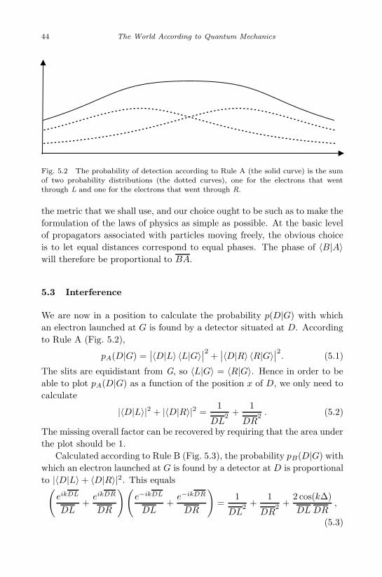
November 24, 2010 10:17 World Scientific Book - 9in x 6in main
44 The World According to Quantum Mechanics
Fig. 5.2 The probability of detection according to Rule A (the solid curve) is the sumof two probability distributions (the dotted curves), one for the electrons that wentthrough L and one for the electrons that went through R.
the metric that we shall use, and our choice ought to be such as to make the
formulation of the laws of physics as simple as possible. At the basic level
of propagators associated with particles moving freely, the obvious choice
is to let equal distances correspond to equal phases. The phase of 〈B|A〉will therefore be proportional to BA.
5.3 Interference
We are now in a position to calculate the probability p(D|G) with which
an electron launched at G is found by a detector situated at D. According
to Rule A (Fig. 5.2),
pA(D|G) =∣∣〈D|L〉 〈L|G〉
∣∣2+∣∣〈D|R〉 〈R|G〉
∣∣2. (5.1)
The slits are equidistant from G, so 〈L|G〉 = 〈R|G〉. Hence in order to be
able to plot pA(D|G) as a function of the position x of D, we only need to
calculate
|〈D|L〉|2 + |〈D|R〉|2 =1
DL2 +
1
DR2 . (5.2)
The missing overall factor can be recovered by requiring that the area under
the plot should be 1.
Calculated according to Rule B (Fig. 5.3), the probability pB(D|G) with
which an electron launched at G is found by a detector at D is proportional
to |〈D|L〉+ 〈D|R〉|2. This equals(
eikDL
DL+eikDR
DR
)(
e−ikDL
DL+e−ikDR
DR
)
=1
DL2 +
1
DR2 +
2 cos(k∆)
DL DR,
(5.3)
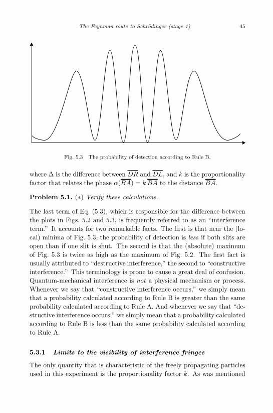
November 24, 2010 10:17 World Scientific Book - 9in x 6in main
The Feynman route to Schrodinger (stage 1) 45
Fig. 5.3 The probability of detection according to Rule B.
where ∆ is the difference between DR and DL, and k is the proportionality
factor that relates the phase α(BA) = k BA to the distance BA.
Problem 5.1. (∗) Verify these calculations.
The last term of Eq. (5.3), which is responsible for the difference between
the plots in Figs. 5.2 and 5.3, is frequently referred to as an “interference
term.” It accounts for two remarkable facts. The first is that near the (lo-
cal) minima of Fig. 5.3, the probability of detection is less if both slits are
open than if one slit is shut. The second is that the (absolute) maximum
of Fig. 5.3 is twice as high as the maximum of Fig. 5.2. The first fact is
usually attributed to “destructive interference,” the second to “constructive
interference.” This terminology is prone to cause a great deal of confusion.
Quantum-mechanical interference is not a physical mechanism or process.
Whenever we say that “constructive interference occurs,” we simply mean
that a probability calculated according to Rule B is greater than the same
probability calculated according to Rule A. And whenever we say that “de-
structive interference occurs,” we simply mean that a probability calculated
according to Rule B is less than the same probability calculated according
to Rule A.
5.3.1 Limits to the visibility of interference fringes
The only quantity that is characteristic of the freely propagating particles
used in this experiment is the proportionality factor k. As was mentioned

November 24, 2010 10:17 World Scientific Book - 9in x 6in main
46 The World According to Quantum Mechanics
Fig. 5.4 If the central maximum of Fig. 5.3 is located at C and the difference betweenRD and LD equals λ, then the first maximum to the left of C is located at D.
in Sec. 5.2.3, its constancy ensures that equal distances correspond to equal
phases. Because phases are cyclic with a period of 2π, the particles in this
experiment define a unit of length λ via k = 2π/λ. While distances per se,
unlike meter sticks, are unobservable, this unit of length can be deduced
from the interference pattern produced by the particles. Figure 5.4 shows
how.
But the wavenumber k = 2π/λ associated with a particle is related to
the particle’s momentum via p = ~k, and p is proportional to the particle’s
mass. If the two-slit experiment is performed with particles of greater mass
(other things being equal), λ will be smaller, and the interference maxima
will be more closely spaced as a result (Fig. 5.5). If we keep increasing
the mass of the particles employed, there comes a point beyond which
the maxima can no longer be resolved, for the intervals monitored by real
detectors cannot be made arbitrarily small. Several maxima and minima
will come to lie in the same interval I , so that the relative frequency with
which particles are detected in I will indicate the mean value of pB(D|G)
across I . A plot obtained with insufficiently small detectors will therefore
resemble the solid line in Fig. 5.2. The peculiar behavior predicted by
Rule B will no longer be in evidence. This is another reason why everyday
objects appear to behave in accordance with the laws of classical physics.

November 24, 2010 10:17 World Scientific Book - 9in x 6in main
The Feynman route to Schrodinger (stage 1) 47
Fig. 5.5 An interference pattern obtained with particles of greater mass.
The limit imposed on the observability of interference patterns by the
mass of the objects employed can be raised by using diffraction gratings—
plates containing large numbers of closely spaced slits—instead of a plate
with only two slits [see Arndt et al. (1999); Brezger et al. (2002); Nairz et
al. (2001)]. But the necessity of using closely spaced and hence narrow slits
then limits the size of the objects with which interference can be observed.
5.4 The propagator as a path integral
Let us replace the plate with two slits by a plate with n holes Bk. Instead of
being the sum of two terms, the propagator 〈D|G〉 is now a sum of n terms,
〈D|G〉 =
n∑
k=1
〈D|Bk〉 〈Bk|G〉 . (5.4)
Next, let us replace the plate with n holes by m such plates a distance ∆y
apart. The resulting propagator is
〈D|G〉 =
n∑
k1=1
· · ·n∑
km=1
〈D|Bkm〉 · · · 〈Bk2
|Bk1〉 〈Bk1
|G〉 . (5.5)
Let us drill more holes in each plate, and let us add more plates. And still
more holes, and still more plates. What happens if we drill so many holes
in each plate that the plates are no longer there? What happens is that

November 24, 2010 10:17 World Scientific Book - 9in x 6in main
48 The World According to Quantum Mechanics
the sumn∑
k1=1
· · ·n∑
km=1
gets replaced by an integral∫DC over all paths that lead from from G
to D, and the amplitude
〈D|Bkm〉 · · · 〈Bk2
|Bk1〉 〈Bk1
|G〉 (5.6)
associated with the alternative
G→ Bk1→ Bk2
→ · · · → Bkm→ D (5.7)
gets replaced by a functional Z[C, G → D]. Unlike a function, which has
input slots for a finite number of variables, a functional has an input slot
for a function—in this case the function that describes the path C from G
to D. The resulting propagator is
〈D|G〉 =
∫
DC Z[C, G→ D] . (5.8)
This is not an ordinary (Riemann) integral∫ b
adx f(x), to which each
infinitesimal interval dx makes a contribution proportional to the value
of f(x) inside it, but a path integral, to which each infinitesimal bundle of
paths DC makes a contribution proportional to the value of Z inside it. As
it stands, it is no more than an idea of an idea, albeit a fruitful one, as we
shall see.
Let us note, to begin with, that if a path C consists of two segments C1and C2, the multiplicativity of successive propagators, Eq. (5.4), translates
to
Z[C] = Z[C2]Z[C1] . (5.9)
5.5 The time-dependent propagator
The alternatives considered so far in this chapter were independent of time.
It did not matter when the electron left G, when it passed the slit plate, or
when it was detected at D. The measurements considered were measure-
ments that indicated (or would have indicated if performed) where particles
were detected but not when they were detected. The paths considered in
the previous section were paths in space, not paths in spacetime (Fig. 5.6).
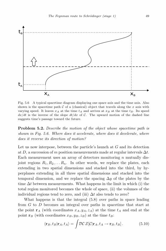
November 24, 2010 10:17 World Scientific Book - 9in x 6in main
The Feynman route to Schrodinger (stage 1) 49
Fig. 5.6 A typical spacetime diagram displaying one space axis and the time axis. Also
shown is the spacetime path C of a (classical) object that travels along the x axis withvarying speed. It leaves xA at the time tA and arrives at xB at the time tB . Its speeddx/dt is the inverse of the slope dt/dx of C. The upward motion of the dashed linesuggests time’s passage toward the future.
Problem 5.2. Describe the motion of the object whose spacetime path is
shown in Fig. 5.6. Where does it accelerate, where does it decelerate, where
does it reverse its direction of motion?
Let us now interpose, between the particle’s launch at G and its detection
atD, a succession ofm position measurements made at regular intervals ∆t.
Each measurement uses an array of detectors monitoring n mutually dis-
joint regions R1, R2, . . . Rn. In other words, we replace the plates, each
extending in two spatial dimensions and stacked into the third, by hy-
perplanes extending in all three spatial dimensions and stacked into the
temporal dimension, and we replace the spacing ∆y of the plates by the
time ∆t between measurements. What happens in the limit in which (i) the
total region monitored becomes the whole of space, (ii) the volumes of the
individual regions tend to zero, and (iii) ∆t also tends to zero?
What happens is that the integral (5.8) over paths in space leading
from G to D becomes an integral over paths in spacetime that start at
the point rA (with coordinates xA, yA, zA) at the time tA and end at the
point rB (with coordinates xB , yB , zB) at the time tB :
〈rB , tB |rA, tA〉 =∫
DC Z[C|rA, tA → rB , tB ] . (5.10)
November 24, 2010 10:17 World Scientific Book - 9in x 6in main
50 The World According to Quantum Mechanics
5.6 A free particle
Now focus on an infinitesimal path dC from x, y, z, t to x + dx, y + dy,
z+dz, t+dt. In general, the amplitude Z(dC) will be a function of x, y, z, t
and dx, dy, dz, dt. In the case of a free particle, however, Z(dC) can de-
pend neither on the location of dC in spacetime (given by the coordinates
x, y, z, t) nor on the orientation of dC in spacetime (given by the ratios of
the differentials dx, dy, dz, dt). Z(dC) can only depend on what for the time
being we may call the “length” ds of dC—a function of dx, dy, dz, dt that
we need to determine. For a free particle, then, Z(dC) = Z(ds).
The multiplicativity of successive propagators, Eq. (5.9), now translates
to
Z(ds1 + ds2) = Z(ds1)Z(ds2) . (5.11)
As we observed in Sec. 3.5, any function satisfying this equation has the
form f(x) = ax. It follows that Z(ds) is of the form ads or, if we introduce
a complex number z such that a = ez,
Z(ds) = ez ds. (5.12)
Equation (5.11) now takes the form
ez(ds1+ds2) = ez ds1 ez ds2 . (5.13)
If instead of combining two infinitesimal path segments we combine all
infinitesimal segments that make up a spacetime path C, we obtain the
amplitude associated with C:
Z[C] (1)=∏
CZ(dC) (2)
=∏
CZ(ds)
(3)=∏
Cez ds (4)
= ez∫
Cds (5)
= ezs[C]. (5.14)
The first equality generalizes Eq. (5.9). The product∏
C multiplies the
infinitely many amplitudes associated with the infinitesimal segments that
make up C. The second equality holds for a free particle. The third follows
from Eq. (5.12). The fourth generalizes Eq. (5.13). The integral∫
C ds,which adds up the “lengths” of the infinitesimal segments that make up C,equals the “length” s[C] of C; this accounts for the fifth equality.
5.7 A free and stable particle
We proceed to calculate the probability with which a free particle detected
at rA at the time tA still exists at the time tB . For a stable free particle
December 23, 2010 9:50 World Scientific Book - 9in x 6in main
The Feynman route to Schrodinger (stage 1) 51
this must be equal to unity. We obtain this probability by integrating the
absolute square of the propagator (5.10) (as a function of rB) over the
whole of space, with Z[C] replaced by ez s[C|rA,tA→rB ,tB ]:∫
|〈rB , tB|rA, tA〉|2 d3rB =
∫ ∣∣∣∣
∫
DC ez s[C|rA,tA→rB ,tB ]
∣∣∣∣
2
d3rB . (5.15)
If you contemplate this with a calm heart and an open mind, you will
notice that if the complex number z = a + ib had a real part a 6= 0, the
path integral would contain a factor ea s[C|rA,tA→rB ,tB ], and the integral
over space, considered as a function of tB, would blow up exponentially (if
a > 0) or fall off exponentially (if a < 0). It could not remain equal to
unity. For a free and stable particle, therefore, z is an imaginary number
ib, and the amplitude associated with a path C is
Z[C|rA, tA → rB, tB ] = eibs[C|rA,tA→rB ,tB ] . (5.16)
The behavior of a free and stable particle thus is controlled by a single real
number b. To discover its significance, we need to know more about the
“length” functional s[C], and to this end we need to acquaint ourselves with
the special theory of relativity.

November 24, 2010 10:17 World Scientific Book - 9in x 6in main
This page intentionally left blankThis page intentionally left blank

November 24, 2010 10:17 World Scientific Book - 9in x 6in main
Chapter 6
Special relativity in a nutshell
6.1 The principle of relativity
Let us imagine a universe containing a single object. Would we be able
to attribute to this object a position—to say where it is? Of course we
wouldn’t. At a minimum we need two objects for this. If we have two ob-
jects, as well as a method of measuring their distance, we can attribute to
them a distance, so we can say how far one is from the other. We can imag-
ine a straight line from one to the other, but if this is all there is, we cannot
attribute to this line an orientation. The bottom line: there is no such thing
as an absolute position or orientation. Positions and orientations are rela-
tive. If we want to make physical sense, we can only speak of the positions
and orientations of physical objects relative to other physical objects.
By the same token, if we were to imagine a world in which a single event
takes place, we would not be able to attribute to this event a time—to say
when it occurs. At a minimum we need two events for this. If we have two
events, as well as a method of measuring the time interval between them,
we can say how much time has passed between them. So there is no such
thing as an absolute time either. If we want to make physical sense, we can
only speak of the times of physical events relative to other physical events.1
And if we were to again imagine a world containing a single object, we
wouldn’t be able to attribute to this object a velocity—to say how fast it
1While one may think of the Big Bang as the beginning of time, this singular eventtranscends the local physics we are concerned with at present. “Local” is used here inthe same sense in which we say that a curve is locally straight or a warped surface islocally flat—the curvature of a sufficiently small segment of a line or patch of a surfacecan be ignored. While spacetime itself may be and, in a sense, is warped, the specialtheory of relativity deals with regions of spacetime that are so small or so weakly warpedthat their curvature need not be taken into account.
53

November 24, 2010 10:17 World Scientific Book - 9in x 6in main
54 The World According to Quantum Mechanics
was moving, in which direction it was moving, or even if it was moving at
all. So there is no such thing as absolute rest either. If we want to make
physical sense, we can only speak of the velocities with which physical
objects move relative to each other.
All of this is encapsulated in the principle of relativity, according to
which all inertial coordinate systems are created equal : the laws of physics
do not “favor” any particular inertial frame or class of such frames.
A coordinate system or frame is inertial if (and only if) the components
x, y, z of the position of any freely moving classical object change by equal
amounts ∆x,∆y,∆z in equal time intervals ∆t. In other words, the ratios
formed of ∆x,∆y,∆z and ∆t are constants. Hence if F is an inertial frame,
then so is any coordinate frame that, relative to F ,
• is shifted (“translated”) in space by a given distance in a given direction,
• is shifted (“translated”) in time by a given amount of time,
• is rotated by a given angle about a given axis, and/or
• moves with a constant velocity.
6.2 Lorentz transformations: General form
The task now before us is to express the coordinates t and r = (x, y, z) of
an inertial frame F1 in terms of the coordinates t′ and r′ = (x′, y′, z′) of
another inertial frame F2. We will make the following assumptions:
• The coordinate origins of the two frames coincide:
t′ = 0 and r′ = 0 mark the same spacetime location as t = 0 and r = 0.
• The spatial axes of the two frames are parallel.
• F2 moves with a constant velocity w relative to F1.
Whatever moves with a constant velocity in one inertial frame will do so in
any other inertial frame. This means that the transformation from t, r to
t′, r′ maps straight lines onto straight lines (in spacetime). Such a transfor-
mation is linear: the dashed coordinates t′, x′, y′, z′ are linear combinations
of the undashed ones:
t′ = a00t+ a01x+ a02y + a03z ,
x′ = a10t+ a11x+ a12y + a13z ,
y′ = a20t+ a21x+ a22y + a23z ,
z′ = a30t+ a31x+ a32y + a33z . (6.1)

November 24, 2010 10:17 World Scientific Book - 9in x 6in main
Special relativity in a nutshell 55
To determine the coefficients aik, we cast these equations into the fol-
lowing form:
t′ = A t+ B · r,r′ = C r + (D · r)w + E t . (6.2)
The real number A is the same as a00, the vector B has the components
(a01, a02, a03), and the vector E has the components (a10, a20, a30). The
part of r′ that is linear in r must be constructed out of the only available
vectors, namely w and r itself. It therefore has two components, one parallel
to r and one parallel to w. Because the component parallel to w must also
be linear in r, its coefficient must be a scalar product formed out of r and
another vector D.
Our next order of business is to find the real numbers A and C and the
vectors B, D, and E. They can only depend on w. More specifically, A
and C must be functions of the magnitude w of w, and B, D, and E must
be parallel to w with magnitudes depending solely on w. Thus,
t′ = a(w) t+ b(w)w · r , (6.3)
r′ = c(w) r +d(w)
w2(w · r)w + e(w)w t . (6.4)
Problem 6.1. What is achieved by the division by w2 in the second term
on the right-hand side of Eq. (6.4)?
We obtain our first constraint on the five functions of w by considering an
object O whose position relative to F1 is given by r = wt, so that
r′ = [c(w) + d(w) + e(w)]w t .
Because both O and F2 move with velocity w relative to F1, O is actually
at rest in F2. Hence
c(w) + d(w) + e(w) = 0 . (6.5)
To obtain further constraints, we make use of the inverse transformation.
Since F1 moves with velocity −w relative to F2, this is given by
t = a(w) t′ − b(w)w · r′ , (6.6)
r = c(w) r′ +d(w)
w2(w · r′)w − e(w)w t′ . (6.7)
We now simplify matters further by choosing the space axes so that w has
the components (w, 0, 0). Equations (6.3) and (6.4) then reduce to
t′ = at+ bwx , x′ = cx+ dx + ewt , y′ = cy , z′ = cz , (6.8)

November 24, 2010 10:17 World Scientific Book - 9in x 6in main
56 The World According to Quantum Mechanics
while Eqs. (6.6) and (6.7) reduce to
t = at′ − bwx′ , x = cx′ + dx′ − ewt′ , y = cy′ , z = cz′ . (6.9)
Plugging Eqs. (6.8) into Eqs. (6.9), we obtain
t = a (at+ bwx) − bw (cx+ dx+ ewt)
= (a2 − bew2) t+ (abw − bcw − bdw)x , (6.10)
x = c (cx+ dx+ ewt) + d (cx+ dx+ ewt)− ew (at+ bwx)
= (c2 + 2cd+ d2 − bew2)x+ (cew + dew − aew) t , (6.11)
y = c2y , (6.12)
z = c2z . (6.13)
To satisfy Eq. (6.10), we must have that
a2 − bew2 = 1 , (6.14)
abw − bcw − bdw = 0 , (6.15)
and to satisfy Eq. (6.11), we must have that
c2 + 2 cd+ d2 − bew2 = (c+ d)2 − bew2 = 1 , (6.16)
cew + dew − aew = 0 . (6.17)
Using Eq. (6.5) and the fact that w 6= 0, the last four equations reduce to
a2 − bew2 = 1 , (6.18)
b(a+ e) = 0 , (6.19)
e2 − bew2 = 1 , (6.20)
e(e+ a) = 0 . (6.21)
Equation (6.20) implies that e 6= 0. With this, Eq. (6.21) tells us that
e = −a. Equation (6.18) then implies that b = (1 − a2)/aw2. From
Eq. (6.12) or (6.13) we learn that c2 = 1, but since we have assumed
that the space axes of the two reference frames are parallel (rather than
antiparallel), we conclude that c = 1. Invoking once more Eq. (6.5), we
find that d = a− 1. With a single unknown function left, Eq. (6.8) reduces
to
t′ = a(w) t +1− a2(w)
a(w)wx , (6.22)
x′ = a(w)x − a(w)wt, y′ = y, z′ = z . (6.23)

November 24, 2010 10:17 World Scientific Book - 9in x 6in main
Special relativity in a nutshell 57
A further constraint can be obtained by combining two such transforma-
tions. If F3 moves with the speed v relative to F2, the transformation from
F2 to F3 is given by
t′′ = a(v) t′ +1− a2(v)
a(v) vx′ , (6.24)
x′′ = a(v)x′ − a(v) vt′, y′′ = y′, z′′ = z′ . (6.25)
Plugging (6.24) and (6.25) into (6.22) and (6.23) yields
t′′ = a(v)
[
a(w) t+1− a2(w)
a(w)wx
]
+1− a2(v)
a(v) v
[a(w)x − a(w)wt
]
=
[
a(v) a(w) − 1− a2(v)
a(v) va(w)w
]
︸ ︷︷ ︸
?
t+[. . .]x , (6.26)
x′′ = a(v)[a(w)x − a(w)wt
]− a(v) v
[
a(w) t+1− a2(w)
a(w)wx
]
=
[
a(v) a(w) − a(v) v 1− a2(w)
a(w)w
]
︸ ︷︷ ︸
?
x−[. . .]t . (6.27)
Another way of writing (6.26) and (6.27) is
t′′ = a(u)︸︷︷︸
?
t+1− a2(u)
a(u)ux , (6.28)
x′′ = a(u)︸︷︷︸
?
x− a(u)ut, y′ = y, z′ = z , (6.29)
where u is the speed of F3 relative to F1. The expressions marked by a
star must be equal; hence
a(u) = a(v) a(w)− 1 − a2(v)
a(v) va(w)w = a(v) a(w)−a(v) v 1 − a2(w)
a(w)w, (6.30)
and thus
KDef=
1− a2(w)
a2(w)w2=
1− a2(v)
a2(v) v2. (6.31)
Since this holds for arbitrary w and v, K is a universal constant. Solving
the first equality for a(w), we arrive at
a(w) =1√
1 +Kw2. (6.32)

November 24, 2010 10:17 World Scientific Book - 9in x 6in main
58 The World According to Quantum Mechanics
With this, the transformation (6.8) takes the form
t′ =t+Kwx√1 +Kw2
, x′ =x− wt√1 +Kw2
, y′ = y, z′ = z . (6.33)
Trumpets, please! We managed to reduce five unknown functions to a
single unknown constant. What is more, if K 6= 0, its value depends on
conventional units—those of an inverse velocity squared. We are therefore
left with three physically distinct options:
(i) K = 0 , (ii) K > 0 , (iii) K < 0 .
6.3 Composition of velocities
K = 0 yields the Galilean transformations of Newtonian mechanics:
t′ = t, x′ = x− wt . (6.34)
Problem 6.2. In this case u = v + w.
If K 6= 0, we can use Eqs. (6.30) and (6.31) to obtain
a(u) = a(v) a(w)(1 −Kvw) . (6.35)
Problem 6.3. (∗) In this case
u =v + w
1−Kvw . (6.36)
If K > 0, we can introduce another constant c = 1/√K, which has the
dimension of a velocity, and write
u =v + w
1− vw/c2 . (6.37)
Setting v = w = c/2, we obtain u = (4/3) c : the speed of F3 relative to
F1 is greater than the sum of the speeds of F3 relative to F2 and of F2
relative to F1. As both v and w approach c, u approaches infinity. And if
the product vw is greater than c2, u is negative!
Problem 6.4. Verify these statements.
If K < 0, we can introduce the constant c = 1/√−K, which again has the
dimension of a velocity, and write
u =v + w
1 + vw/c2. (6.38)
November 24, 2010 10:17 World Scientific Book - 9in x 6in main
Special relativity in a nutshell 59
Setting v = w = c/2, we obtain u = (4/5) c : the speed of F3 relative to F1
is less than the sum of the speeds of F3 relative to F2 and of F2 relative to
F1. And if v or w approaches c, then so does u.
Problem 6.5. Verify these statements.
6.4 The case against positive K
Pick an infinitesimal segment dC of a spacetime path C. In terms of F1, it
has the components (dt, dx, dy, dz), and in terms of F2, it has the compo-
nents (dt′, dx′, dy′, dz′). These components, too, are related to each other
via the transformation (6.33):
dt′ =dt+Kwdx√
1 +Kw2, dx′ =
dx− w dt√1 +Kw2
, dy′ = dy , dz′ = dz . (6.39)
Problem 6.6.
dt′2 +K (dx′2 + dy′2 + dz′2) = dt2 +K (dx2 + dy2 + dz2) . (6.40)
If K = 0, this doesn’t tell us anything new.
If K > 0, it is convenient to choose measurement units in which K = 1,
so that distances and durations are measured in the same units. What you
have just proved is that the expression
ds2Def= dt2 + dx2 + dy2 + dz2 (6.41)
is invariant under the transformation (6.39) with K equal to unity.
This should remind you of something. If x, y, z are the components of
a vector r, then the expression x2 + y2 + z2 is invariant under coordinate
transformations that preserve the magnitudes of vectors. Here we have an
analogous expression that is invariant under the transformations (6.39). If
K > 0 were Nature’s choice, we could identify ds as the “length” of the
path segment dC, which we are looking for, as you will recall from (Sec. 5.7).
But is K = 1 a live option? Consult Fig. 6.1. The speed of F2 relative
to F1 is w = tanα. The coordinates of a spacetime vector v in the x–t
plane are therefore related via
t′ =t+ x tanα√1 + tan2 α
, x′ =x− t tanα√1 + tan2 α
. (6.42)
Problem 6.7. (∗)t′ = t cosα+ x sinα , x′ = x cosα− t sinα . (6.43)
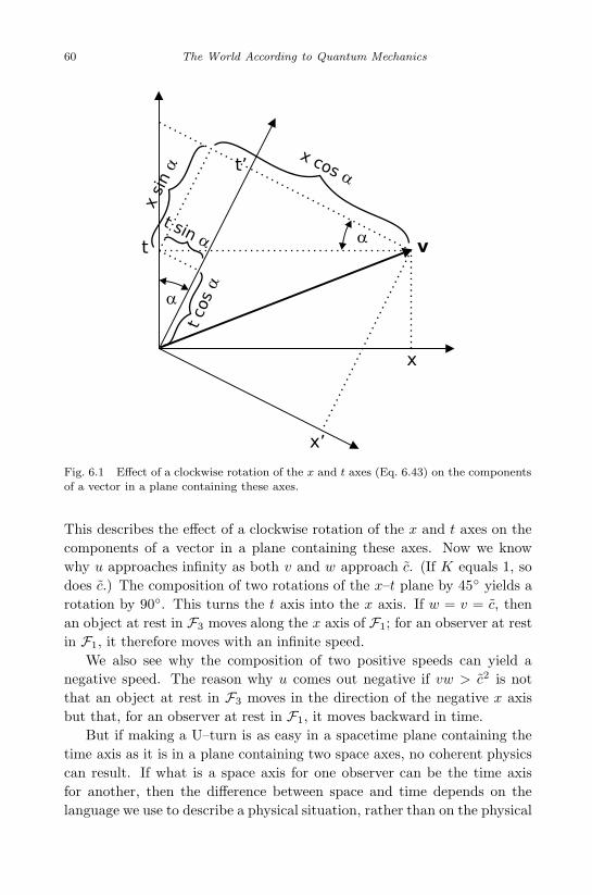
November 24, 2010 10:17 World Scientific Book - 9in x 6in main
60 The World According to Quantum Mechanics
Fig. 6.1 Effect of a clockwise rotation of the x and t axes (Eq. 6.43) on the componentsof a vector in a plane containing these axes.
This describes the effect of a clockwise rotation of the x and t axes on the
components of a vector in a plane containing these axes. Now we know
why u approaches infinity as both v and w approach c. (If K equals 1, so
does c.) The composition of two rotations of the x–t plane by 45◦ yields a
rotation by 90◦. This turns the t axis into the x axis. If w = v = c, then
an object at rest in F3 moves along the x axis of F1; for an observer at rest
in F1, it therefore moves with an infinite speed.
We also see why the composition of two positive speeds can yield a
negative speed. The reason why u comes out negative if vw > c2 is not
that an object at rest in F3 moves in the direction of the negative x axis
but that, for an observer at rest in F1, it moves backward in time.
But if making a U–turn is as easy in a spacetime plane containing the
time axis as it is in a plane containing two space axes, no coherent physics
can result. If what is a space axis for one observer can be the time axis
for another, then the difference between space and time depends on the
language we use to describe a physical situation, rather than on the physical

November 24, 2010 10:17 World Scientific Book - 9in x 6in main
Special relativity in a nutshell 61
situation itself. Yet any viable theory about the physical world must, at
a minimum, feature an objective—i.e., language-independent—difference
between space and time.
Here is one reason why. The stability of an atom—and with it that
of matter—rests crucially on the fuzziness of its internal relative positions
(Sec. 4.3). At the same time the position of an atomic electron relative
to the nucleus cannot be completely fuzzy, for in this case the probabil-
ity per unit volume of detecting it would be constant over the (abstract)
space of sharp positions relative to the nucleus. In other words, the elec-
tron’s position probability distribution (relative to the nucleus) would be
homogeneous. But this cannot be: the electron has to be more likely to
be detected in one place rather than in another. On the other hand, there
has to be a ground state that is homogeneous in time: the probabilities it
defines must not change with time. These two requirements cannot be met
unless there is a language-independent difference between space and time.
6.5 An invariant speed
If K ≤ 0, there exists an invariant speed. (Whatever moves with an invari-
ant speed relative to one inertial frame, moves with the same speed relative
to any other inertial frame.)
To see this, suppose that an object traveling with c relative to F2 also
travels with c relative to F3, regardless of the relative speed v between F2
and F3. Inserting w = c and u = c into Eq. (6.36), we obtain c = 1/√−K.
Thus an invariant speed equal to c exists if K ≤ 0 but not if K > 0.
If K = 0, the invariant speed is infinite: what travels with infinite
speed relative to one inertial frame, travels with infinite speed relative to
every inertial frame. In other words, if the departure of an object and its
arrival are simultaneous in one inertial frame, they are simultaneous in every
inertial frame. In Newtonian mechanics, simultaneity is therefore absolute:
whether or not two events happen at the same time is independent of the
reference frame that we use to describe their spatiotemporal relations.
If K is negative, the invariant speed is finite. Empirically we know that
an invariant speed exists, and that it is finite. We call it the “speed of light
(in vacuum).” Nature’s choice—K < 0—stands thereby revealed.
The invariant speed—be it infinite or finite—cannot be attained by any
object that can be at rest. To see this, imagine that you spend a finite
amount of fuel accelerating from zero to some speed v < c. In the frame in

November 24, 2010 10:17 World Scientific Book - 9in x 6in main
62 The World According to Quantum Mechanics
which you are now at rest, the difference between the invariant speed and
yours is still the invariant speed. You may repeat the procedure as many
times as you wish—the difference between the invariant speed and yours
remains the invariant speed. No finite amount of fuel is sufficient to reach
it. Moreover, since you have to attain the invariant speed before you can
make a U–turn in a plane that contains the time axis, the existence of an
invariant speed is what prevents you from going back in time.
6.6 Proper time
With K = −1/c2, the transformation (6.39) and the invariant expression
(6.40) take the following forms:
t′ =t− wx/c2√
1− w2/c2, x′ =
x− wt√
1− w2/c2, y′ = y , z′ = z , (6.44)
ds2 = dt2 − (dx2 + dy2 + dz2)/c2 . (6.45)
Here at last is the wanted “length” ds of a path segment dC with compo-
nents dt, dx, dy, dz (Sec. 5.7). What is its physical significance?
Imagine a clock that travels along the infinitesimal segment dC of a
spacetime path C.2 The passing of time it shows is the passing of the
coordinate time of the inertial frame in which it is momentarily (i.e., during
an infinitesimal time interval) at rest. To distinguish this time from the
coordinate time of a fixed inertial frame, we refer to it as proper time.3 The
proper time s[C] associated with an entire spacetime path is thus related to
a system of inertial coordinates via∫
Cds =
∫
C
√
dt2 − (dx2 + dy2 + dz2)/c2 =
∫
Cdt√
1− v2/c2 . (6.46)
2A word of caution. Because we cannot help visualizing a plane containing the time axisas a spatial plane, like a figure on a page, we are tempted to think about the spatiotem-poral whole as if it were a 4-dimensional spatial landscape, and about the present—a3-dimensional section of this landscape—as if it advanced through this spatiotemporalwhole. This way of thinking involves an illegitimate duplication of time. First we men-tally represent time as a dimension of a 4-dimensional whole, and then we think of this4-dimensional whole (including its temporal dimension) as a spatial whole that persistsin another temporal dimension, in which the present advances through this now spa-tially conceived whole. So if we say that an object “travels” along a spacetime path,we must take care not to think of this object as traveling along a path in a persistent4-dimensional expanse.3Because we only have ds2 = dt2 (in the momentary rest frame), there are two possi-
bilities: ds = dt and ds = −dt. As we shall see in Sec. 15.2, the former holds for particleswhile the latter holds for antiparticles [Costella et al. (1997)].

November 24, 2010 10:17 World Scientific Book - 9in x 6in main
Special relativity in a nutshell 63
The definition of proper time is restricted to timelike paths. A finite path
is called timelike if every one of its segments is, and an infinitesimal path
segment dC is timelike if ds2 > 0. By the same token, a finite path is
called spacelike if every one of its segments is, and an infinitesimal path
segment dC is spacelike if ds2 < 0. Finally, a finite path is called lightlike
or null if every one of its segments is, and an infinitesimal path segment dCis lightlike or null if ds2 = 0.
Problem 6.8. The speed of an object moving along a timelike path is always
less than the invariant speed c.
Problem 6.9. (∗) Use dt2 − dx2/c2 = (dt′)2 − (dx′)2/c2 to show that c is
an invariant speed.
6.7 The meaning of mass
Now we are ready to address the question left pending in Chap. 5, con-
cerning the significance of the single particle-specific parameter b, which
appears in the propagator for a free and stable particle,
〈rB , tB |rA, tA〉 =
∫
DC eibs[C|rA,tA→rB ,tB ] . (6.47)
If proper time is measured in seconds, b is measured in radians per second.
Let us follow a particle as it travels from A to B along C. As its proper
time s increases, the phase factor eibs rotates in the complex plane. We may
therefore think of it as a clock. Each time a cycle is completed, it “ticks.”
Although a feature of the quantum-mechanical probability calculus rather
than of the physical world, this clock reveals a deep connection between
the quantum-mechanical probability calculus and the metric properties of
the physical world.
It is customary—
• to insert a minus (so that our clock actually turns clockwise!): e−ibs,
• to multiply by 2π (so that we may think of b as the rate at which the
clock “ticks”—the number of cycles it completes each second): e−i 2πbs,
• to divide by Planck’s constant h (so that b is measured in energy units,
in which case it is known as the particle’s rest energy): e−i(2π/h)bs =
e−(i/~)bs,
• to multiply by c2 (so that b is measured in mass units, in which case it
is known as the particle’s mass m): e−(i/~)bc2s = e−(i/~)mc2s.

November 24, 2010 10:17 World Scientific Book - 9in x 6in main
64 The World According to Quantum Mechanics
If we use natural units, in which ~ = c = 1, we are back at e−ibs with
b = m. Thus apart from a factor 2π, which converts between cycles per
second and radians per second, the mass of a particle is the rate at which
the clock associated with the particle ticks.
Now imagine two ordinary clocks initially at rest relative to the same
inertial frame (F1). They are located in about the same place and they
tick at the same rate. They then travel along different spacetime paths.
Eventually they are again at rest relative to the same inertial frame (F2)
and located in about the same place. Will they still tick at the same
rate? Indeed they will, but why? This is not something we should take for
granted. The reason why they still tick at the same rate is that (i) the rates
at which clocks tick depend on the rates at which free particles tick in their
rest frames, (ii) the rate at which a free particle ticks in its rest frame is
determined by its mass, and (iii) the mass of a free particle is independent
of the particle’s location in spacetime.
6.8 The case against K = 0
If K were to vanish, proper time would be the same as coordinate time.
Every spacetime path leading from A to B would contribute the same
amplitude eib (tB−tA) to the propagator (6.47), which would be hopelessly
divergent as a result—as well as independent of the distance between A
and B. To obtain finite probabilities, cancellations (“destructive interfer-
ence”) must occur. The phase factors eibs[C|rA,tA→rB ,tB ] must not all point
in the same direction in the complex plane.
While this does not quite rule out the option K = 0 (after all, there is
such a thing as non-relativistic quantum mechanics), the manner in which
one obtains the non-relativistic substitute for ds makes it clear that this
can only be an approximation—useful to the extent that all powers of v2/c2
but the first can be ignored.
Problem 6.10. Use the Taylor series to show that√
1− v2
c2= 1− 1
2
v2
c2− 1
8
v4
c4− · · · ≈ 1− 1
2
v2
c2. (6.48)
In this approximation, Eq. (6.46) becomes
∫
Cds ≈
∫
Cdt
(
1− 1
2
v2
c2
)
= (tB − tA)− 1
2c2
∫
Cdt v2 , (6.49)

November 24, 2010 10:17 World Scientific Book - 9in x 6in main
Special relativity in a nutshell 65
Fig. 6.2 Spacetime coordinates of an event A relative to two different inertial frames.
and the propagator (6.47) takes the form
〈rB , tB |rA, tA〉 =∫
DC e−(i/~)mc2∫
Cds (6.50)
≈ e−(i/~)mc2(tB−tA)
∫
DC e(i/~)∫
Cdt (mv2/2) . (6.51)
Since the phase factor e−(i/~)mc2(tB−tA) is the same for all paths from A
to B, it has no effect on the probabilities that the propagator serves to cal-
culate. Hence the following may be used as the non-relativistic propagator:
〈rB , tB |rA, tA〉 =∫
DC e(i/~)∫
Cdt (mv2/2). (6.52)
6.9 Lorentz transformations: Some implications
Let us explore, briefly, what is implied by the Lorentz transformation (6.44).
We shall use units in which c = 1.
Setting t′ = 0, we obtain t = wx. This tells us that the slope of the
x′ axis in the x–t frame (F1) equals w. Setting x′ = 0, we obtain t = x/w.

November 24, 2010 10:17 World Scientific Book - 9in x 6in main
66 The World According to Quantum Mechanics
Fig. 6.3 The unit points of the space and time axes are situated on hyperbolas.
This tells us that the slope of the t′ axis in the x–t frame is the inverse:
1/w. The axes of F2 are thus rotated relative to F1 by equal angles but
in opposite directions (Fig. 6.2). The spacetime path of a (classical) light
signal traveling in the direction defined by the x axis is therefore the bisector
of the angle between the x and t axes of both frames.
The big news here is that simultaneity is relative. Events that happen
at the same time in a given frame can be connected by a line parallel to
the frame’s space axis, just as events that happen in the same place in a
given frame can be connected by a line parallel to the frame’s time axis.
This is true in any case. But since in this case the space axes of the two
frames are not parallel, whether or not two events are simultaneous depends
on the language—the inertial reference frame—that we use to describe a
physical situation, rather than on the physical situation itself. If two events
E1, E2 are simultaneous relative to one frame, there are frames relative to
which E1 happens after E2 as well as frames relative to which E1 happens
before E2.

November 24, 2010 10:17 World Scientific Book - 9in x 6in main
Special relativity in a nutshell 67
Fig. 6.4 Lorentz contraction.
Next we want to determine the unit points on the space and time axes
of the two inertial frames of Fig. 6.2. To this end we use the invariant
expression
t2 − x2 = t′2 − x′2 .
The unit point of the time axis of F2 has the coordinates t′ = 1, x′ = 0; it
therefore lies on the hyperbola defined by t2 − x2 = 1. The unit point of
the space axis of F2 has the coordinates t′ = 0, x′ = 1; it therefore lies on
the hyperbola defined by x2 − t2 = 1 (Fig. 6.3).
Figure 6.4 illustrates the phenomenon of Lorentz contraction: a moving
object is shortened in the direction in which it is moving. The graph on
the left shows the spacetime area traced by a meter stick at rest in F1. In
F2, in which the stick is moving, it is shorter: the distance between its end
points on the x′ axis is less than a meter. The graph on the right shows
the spacetime area traced by a meter stick at rest in F2. In F1, in which
this stick is moving, it is shorter: the distance between its end points on
the x axis is again less than a meter.
Figure 6.5 illustrates the phenomenon of time dilation: a moving clock
runs slower than a clock at rest. Let clock 1 be at rest in F1, its spacetime
path being the t axis. Let clock 2 be at rest in F2, its spacetime path
being the t′ axis. In the language of F1, when a second has passed (on
clock 1), less than a second has passed on clock 2. In the language of F2,
when a second has passed (on clock 2), less than a second has passed on
clock 1.

November 24, 2010 10:17 World Scientific Book - 9in x 6in main
68 The World According to Quantum Mechanics
Fig. 6.5 Time dilation.
6.10 4-vectors
For later use we still need to define 4-vectors and their scalar product. A
4-vector is a quadruplet of real numbers that changes like the coordinates
of a point in spacetime when subjected to a Lorentz transformation. The
scalar product of the 4-vectors~a = (at, a) = (a0, a1, a2, a3) and~b = (bt,b) =
(b0, b1, b2, b3) is
(~a,~b)Def= a0b0 − a1b1 − a2b2 − a3b3 . (6.53)
To check that (~a,~b) is invariant under Lorentz transformations, we consider
the sum of two 4-vectors, ~c = ~a+~b, and calculate
(~c,~c) = (~a+~b,~a+~b) = (~a,~a) + (~b,~b) + 2(~a,~b) . (6.54)
Because the expression (6.45) is invariant under the transformation (6.44),
the “squares” (~a,~a), (~b,~b) and (~c,~c) are so, too (c = 1 was assumed). But
if these are invariant, then so is the last term on the right-hand side of
Eq. (6.54). In other words, (~a,~b) is a 4-scalar.

December 23, 2010 9:50 World Scientific Book - 9in x 6in main
Chapter 7
The Feynman route to Schrodinger(stage 2)
7.1 Action
Let us return to Eq. (5.9). For an infinitesimal path made up of two seg-
ments, this takes the form
Z(dC) = Z(dC2)Z(dC1) . (7.1)
In Sec. 5.6 we noted that, in the general case, Z(dC) is a function of the
spacetime position of dC and of the coordinate differentials (dt, dr). Equa-
tion (7.1) is therefore tantamount to
Z(t, r, dt1 + dt2, dr1 + dr2) = Z(t, r, dt2, dr2)Z(t, r, dt1, dr1) . (7.2)
From this we conclude—by the same reasoning we used in Sec. 5.6—that
the amplitude associated with an infinitesimal path segment takes the form
Z(t, r, dt, dr) = ez dS(t,r,dt,dr). (7.3)
We further conclude—by the same reasoning we used in Sec. 5.7—that
for a stable particle the complex number z = a + ib has to be imaginary
(a = 0). It is customary to set b = 1/~, so that the infinitesimal action dS is
measured in conventional units (energy × time or momentum × distance):
Z(t, r, dt, dr) = e(i/~)dS(t,r,dt,dr). (7.4)
A glance at Eq. (6.50) now reveals the action differential for a free and
stable particle:
dS = −mc2ds . (7.5)
Equation (7.2) can be generalized to read
Z(t, r, u dt, u dr) = [Z(t, r, dt, dr)]u. (7.6)
69

November 24, 2010 10:17 World Scientific Book - 9in x 6in main
70 The World According to Quantum Mechanics
In conjunction with Eq. (7.4) this tells us that
dS(t, r, u dt, u dr) = u dS(t, r, dt, dr) . (7.7)
Technically this makes dS homogeneous (of first degree) in the differentials
dt and dr. This homogeneity allows us to interpret dS as defining a differ-
ential geometry—the kind of geometry one needs for assigning lengths to
paths on a warped surface, in a warped space, or in a warped spacetime.
7.2 How to influence a stable particle?
Suppose now that something—no matter what—exerts an influence—no
matter how—on a stable particle. How do we incorporate effects on the
motion of such a particle? Since all we have at our disposal is the lengths
of paths as defined by this differential geometry, the only way in which we
can formulate effects on the particle’s motion is through modifications of dS.
Since the action differential encapsulates the particle’s observable behavior,
it is moreover essential that it be invariant under Lorentz transformations.
It must not depend on the language—the reference frame—that we use to
describe the particle’s behavior. The scope of possible effects on the motion
of a particle is therefore limited to modifications of the action differential
(7.5) that preserve
(1) the homogeneity expressed by Eq. (7.7),
(2) the invariance of dS as a 4-scalar.
One possible modification that meets these requirements stands out as the
most obvious and straightforward: to preserve Lorentz invariance, we add
to (7.5) the scalar product (6.53) of two 4-vectors, and to preserve homo-
geneity, we let one of these vectors be d~r = (c dt, dr). We shall denote
the other vector, whose components are in general functions of t and r, by~A = (V,A). The inclusion of a charge q allows the extent to which particles
are affected to differ between particle species. Thus:
dS = −mc2 ds− qV (t, r) dt+q
cA(t, r) · dr . (7.8)
Here Gaussian units are used. In SI units the factor 1/c is absorbed into
the definition of A:
dS = −mc2 ds− qV (t, r) dt + qA(t, r) · dr . (7.9)
As we shall see in Sec. 9.5, the fields V and A uniquely determine the
classical electric field E and the classical magnetic field B. In other words,

November 24, 2010 10:17 World Scientific Book - 9in x 6in main
The Feynman route to Schrodinger (stage 2) 71
the action differential (7.8) encapsulates the effects of the electromagnetic
force.1
7.3 Enter the wave function
In the non-relativistic approximation, the action differential (7.5) for a free
particle takes the form
dS =m
2v2 dt , (7.10)
as we gather from Eq. (6.52). If the vector potential vanishes or is small
enough to be ignored, and if we are dealing with a particle of unit charge
(q = 1), then the action differential (7.8) takes the simple form
dS =(m
2v2 − V
)
dt . (7.11)
We now introduce a function ψ(t, r) such that
ψ(rB , tB) =
∫
d3rA 〈rB , tB |rA, tA〉ψ(rA, tA) . (7.12)
Using the path–integral form of the propagator 〈rB , tB |rA, tA〉,∫
DC e(i/~)∫
CdS , (7.13)
with the action differential (7.11), we arrive at
ψ(rB , tB) =
∫
d3rA
[∫
DC e(i/~)∫
C[(m/2)v2−V ]dt
]
ψ(rA, tA) . (7.14)
7.4 The Schrodinger equation
We obtain a more user-friendly expression to work with by considering
an infinitesimal time interval tB − tA = ε. In this case there is just one
(infinitesimal) path connecting (tA, rA) and (tB , rB), and all that remains
of the path integral is an as yet unknown normalization factor N :
ψ(rB , t+ ε) = N∫
d3rA e(i/~)[(m/2)v2−V ]ε ψ(rA, t) . (7.15)
1Strictly speaking, Eq. (7.8) encapsulates the possible electromagnetic effects on theobservable behavior of a scalar particle. By this we mean a particle whose wave functionhas a single component. This excludes particles with spin (Chap. 12) and particles thatare affected by nuclear forces (Sec. 15.9).

November 24, 2010 10:17 World Scientific Book - 9in x 6in main
72 The World According to Quantum Mechanics
To further simplify our lives, we return to one spatial dimension,
ψ(xB , t+ ε) = N∫ +∞
−∞dxA e
(i/~)[(m/2)((xb−xA)2/ε2)−V ]ε ψ(xA, t) , (7.16)
and we substitute η for xA − xB (and drop the now superfluous index B):
ψ(x, t+ ε) = N∫ +∞
−∞dη e(i/~)[(m/2)(η2/ε2)−V ]ε ψ(x + η, t) . (7.17)
Take a look at the exponential factor eimη2/2~ε. In the limit ε → 0, this
completes an infinite number of cycles as η increases by a finite amount
unless η2 is of the same order of magnitude as ε. Unless this is the case, the
remaining factors of the integrand—e−iεV/~ and ψ(x+η, t)—can be treated
as constant during a cycle, so that the net contribution to the integral from
such a cycle is zero. Hence in order to take the limit ε → 0, we need to
expand e−iεV/~ ψ(x+ η, t) to the first power of ε or to the second power of
η:
e−iεV/~ ψ(x+ η, t) ≈(
1− iεV
~
)(
ψ(t, x) +∂ψ
∂xη +
∂2ψ
∂x2
η2
2
)
≈(
1− iεV
~
)
ψ(t, x) +∂ψ
∂xη +
∂2ψ
∂x2
η2
2. (7.18)
The following integrals need to be evaluated:
I1 =
∫
dη eimη2/2~ε, I2 =
∫
dη eimη2/2~εη , I3 =
∫
dη eimη2/2~εη2.
I2 vanishes because the integrand is antisymmetric: the integral over the
interval from −∞ to 0 is the negative of the integral over the interval from 0
to +∞. Using Eq. (3.28) we find that I1 =√
2πi~ε/m, and using Eq. (3.29)
we find that I3 =√
2π~3ε3/im3. Putting everything together, we arrive at
ψ(x, t) +∂ψ
∂tε = N
√
2πi~ε
m
(
1− iε
~V (x, t)
)
ψ(x, t) +N2
√
2π~3ε3
im3
∂2ψ
∂x2.
(7.19)
For the two sides to be equal as ε tends to zero, we must have that N =√
m/2πi~ε. Equation (7.19) therefore reduces to
∂ψ
∂t= − i
~V (x, t)ψ(x, t) +
i~
2m
∂2ψ
∂x2. (7.20)
November 24, 2010 10:17 World Scientific Book - 9in x 6in main
The Feynman route to Schrodinger (stage 2) 73
Since ε has dropped out, all that remains to be done is multiply both sides
with i~. The result is the standard form of the Schrodinger equation for
a particle of unit charge with one degree of freedom, moving under an
influence represented by the potential V (t, x) (cf. Eq. 4.4):
i~∂ψ
∂t= − ~
2
2m
∂2ψ
∂x2+ V ψ . (7.21)
Introducing the differential operator ∂/∂r—a machine that ac-
cepts a function f(r) and returns a vector with the components
(∂f/∂x, ∂f/∂y, ∂f/∂z)—we can write the corresponding equation for a
particle of charge q with three degrees of freedom in the following way
(cf. Eq. 4.5):(
i~∂
∂t− qV
)
ψ =1
2m
(~
i
∂
∂r
)
·(
~
i
∂
∂r
)
ψ . (7.22)
As we shall see in Sec. 11.6, i~(∂/∂t) is the operator associated with the
particle’s total energy, and (~/i)(∂/∂r) is the operator associated with the
particle’s total momentum. (See Sec. 11.2 for the reason why operators
are associated with observables.) On the left-hand side we thus have the
operator for the particle’s kinetic energy. The inclusion of the particle’s
potential momentum (q/c)A (see Eq. 9.20) is straightforward:(
i~∂
∂t− qV
)
ψ =1
2m
(~
i
∂
∂r− q
cA
)
·(
~
i
∂
∂r− q
cA
)
ψ . (7.23)

November 24, 2010 10:17 World Scientific Book - 9in x 6in main
This page intentionally left blankThis page intentionally left blank

November 24, 2010 10:17 World Scientific Book - 9in x 6in main
PART 2
A Closer Look
75

November 24, 2010 10:17 World Scientific Book - 9in x 6in main
76
This page intentionally left blankThis page intentionally left blank

November 24, 2010 10:17 World Scientific Book - 9in x 6in main
Chapter 8
Why quantum mechanics?
8.1 The classical probability calculus
An exhaustive description of a classical physical system at any one time
consists of the values of a fixed number N of coordinates and an equal
number of momenta. Such a description is usually referred to as the sys-
tem’s state, and the system is said to have N degrees of freedom. This
makes it possible to treat the state of a classical system with N degrees of
freedom as a point P in a 2N -dimensional space S known as phase space.
As an example consider the classical harmonic oscillator (Fig. 8.1). It
has one degree of freedom, a 2-dimensional phase space, and the following
equation of motion:
md2x
dt2= −kx . (8.1)
Problem 8.1. In Fig. 8.1, which way does the oscillator’s state P move?
Clockwise or counterclockwise?
Now for some truisms. A physical theory is as good as its predictions, and
what quantum mechanics predicts are measurement outcomes. Moreover,
with the exception of measurements that have finite sets of possible out-
comes, no real-world experiment has an exact outcome. (Otherwise one
could experimentally establish whether a physical quantity with a contin-
uous range of possible values has a rational rather than irrational value.)
If measurement outcomes are digitally displayed, as may reasonably be as-
sumed, then every measurement has a finite number of possible outcomes.
A (successful) measurement is therefore equivalent to a finite number of
simultaneous measurements each having two possible outcomes. We will
call such a measurement an elementary test. An elementary test associated
77

November 24, 2010 10:17 World Scientific Book - 9in x 6in main
78 The World According to Quantum Mechanics
Fig. 8.1 Phase space diagram of a harmonic oscillator. Observe that when |x| is at amaximum, p changes its sign (the oscillator reverses its motion), and when x = 0, |p| isat a maximum (the oscillator moves fastest). See the main text for the significance ofthe gray strips.
with a continuous physical quantity X typically answers the question: does
the value of X lie in the interval I? If the possible outcomes of a measure-
ment are the intervals Ik , k = 1, . . . , n, the outcome of one elementary test
will be positive, while those of the remaining n− 1 tests will be negative.
In our oscillator example, intervals of the x axis and intervals of the
p axis are some of the possible outcomes of elementary tests. In the system’s
phase space, the former intervals correspond to vertical strips, the latter to
horizontal strips, as indicated in Fig. 8.1. The intersection of a horizontal
and a vertical strip corresponds to the outcome of another elementary test,
determining the simultaneous truth of the propositions “the value of x
lies in the vertical strip” and “the value of p lies in the horizontal strip.”
Generalizing this possibility by allowing every subset of phase space to
be the possible outcome of an elementary test, we arrive at the following
characterization of the classical probability calculus.
• An elementary test is (represented by) a subset U of a phase space S.
• The algorithm that serves to assign probabilities to the outcomes of
elementary tests is a point P in S.
• The probability of obtaining a positive outcome for U is 1 if U con-
tains P (in set-theoretic notation, P ∈ U).
• The probability of obtaining a positive outcome for U is 0 if U does not
contain P (P 6∈ U).

November 24, 2010 10:17 World Scientific Book - 9in x 6in main
Why quantum mechanics? 79
This probability algorithm is trivial, in the sense that it only assigns
trivial probabilities: 0 or 1. Because it is trivial, P can be thought of as a
state in the classical sense of the word: a collection of possessed properties.
We are licensed to believe that U represents a physical property (rather than
an elementary test), and that if the probability of finding this property is 1,
it is because the system possesses the property, irrespective of whether the
corresponding elementary test is made.
8.2 Why nontrivial probabilities?
One of the most spectacular failures of classical physics was its inability to
account for the stability of matter. “Ordinary” material objects
• have spatial extent (they “occupy space”),
• are composed of a (large but) finite number of objects without spatial
extent (particles that do not “occupy space”),
• and are stable (they neither explode nor collapse as soon as they are
created).
Ordinary objects occupy as much space as they do because atoms and
molecules occupy as much space as they do. So how is it that a hydrogen
atom in its ground state occupies a space roughly one tenth of a nano-
meter across? Thanks to quantum mechanics, we now understand that the
stability of ordinary objects rests on the indeterminacy or fuzziness of the
relative positions and momenta of their constituents (Sec. 4.3).
What, then, is the proper (i.e., mathematically rigorous and philosoph-
ically sound) way to define and quantify a fuzzy property or value? It is
to assign nontrivial probabilities—probabilities between 0 and 1—to the
possible outcomes of a measurement of this property. To be precise, the
proper way of quantifying a fuzzy property or value is to make counterfac-
tual probability assignments. (To assign a probability to a possible mea-
surement outcome counterfactually—contrary to the facts—is to assign it
to a possible outcome of a measurement that is not actually made.) In
order to quantitatively describe a fuzzy observable, we must assume that
a measurement is made, and if we do not want our description to change
the observable described, we must assume that no measurement is made.
We must assign probabilities to the possible outcomes of unperformed
measurements.

November 24, 2010 10:17 World Scientific Book - 9in x 6in main
80 The World According to Quantum Mechanics
8.3 Upgrading from classical to quantum
The classical probability algorithm cannot accommodate the nontrivial
probabilities that are needed for the purpose of defining and quantifying
a fuzzy physical property. Nor can the probability algorithms of classical
statistical physics be used for this purpose, for the nontrivial probabilities
of classical physics are distributions over a phase space, and this makes
them consistent with the belief that the real (albeit unknown) state is rep-
resented by a point P in this space. In other words, the probabilities of
classical statistical physics are (or allow themselves to be thought of as)
ignorance probabilities. They enter the picture when relevant facts are ig-
nored, and they disappear, or degenerate into trivial probabilities, when all
relevant facts are taken into account. The “uncertainty” relation (4.18), on
the other hand, guarantees that quantum-mechanical probabilities cannot
be made to disappear.
Arguably the most straightforward way to make room for nontrivial
probabilities is to upgrade1 from a 0-dimensional point P to a 1-dimensional
line L. Instead of representing a probability algorithm by a point in a phase
space, we represent it by a 1-dimensional subspace of a vector space V .
(Such a subspace is sometimes called a “ray.”) And instead of represent-
ing elementary tests by subsets of a phase space S, we represent them by
the subspaces of V . A 1-dimensional subspace L can be contained in a
subspace U , it can be orthogonal to U (L ⊥ U), but it may be neither
contained in nor orthogonal to U ; there is a third possibility, and this is
what makes room for nontrivial probabilities. L assigns probability 1 to
elementary tests represented by subspaces containing L, it assigns proba-
bility 0 to elementary tests represented by subspaces orthogonal to L, and
it assigns probabilities greater than 0 and less than 1 to tests represented
by subspaces that neither contain nor are orthogonal to L.
8.4 Vector spaces
Using the notation introduced by Paul Dirac, we define a vector space Vas a set of vectors |a〉, |b〉, |c〉. . . that can be (i) added and (ii) multiplied
with real or complex numbers α, β, γ. . . . The result of either operation is
another vector in V . There is a null vector |0〉 such that for any vector |a〉we have |a〉 + |0〉 = |a〉 and 0 |a〉 = |0〉. If in addition (as we shall assume)
1The virtual inevitability of this “upgrade” was demonstrated by Jauch (1968).

November 24, 2010 10:17 World Scientific Book - 9in x 6in main
Why quantum mechanics? 81
V comes equipped with an inner or scalar product—a machine that accepts
two vectors |a〉, |b〉 and returns a real or complex number 〈a|b〉, then V is an
inner product space. In a real vector space, only real numbers are admitted,
and the scalar product is symmetric as well as linear in both vectors. This
means that
〈a|b〉 = 〈b|a〉 , (8.2)
if |A〉 = α|a〉 and |B〉 = β|b〉 then 〈A|B〉 = αβ〈a|b〉 . (8.3)
In a complex vector space, these requirements are replaced by
〈a|b〉 = 〈b|a〉∗, (8.4)
if |A〉 = α|a〉 and |B〉 = β|b〉 then 〈A|B〉 = α∗β〈a|b〉 . (8.5)
Problem 8.2. The last two requirements follow from the demand that 〈a|a〉be a real number.
In addition we have that
if |c〉 = |a〉+ |b〉 then 〈d|c〉 = 〈d|a〉+ 〈d|b〉 , (8.6)
〈a|a〉 ≥ 0 , (8.7)
if 〈a|a〉 = 0 then |a〉 = |0〉 . (8.8)
A few more definitions are needed:
• Two vectors are (mutually) orthogonal if their scalar product vanishes.
• A set of vectors |a1〉, . . . , |am〉 is linearly independent if α1|a1〉+ · · ·+αm|am〉 = 0 implies that α1 = · · · = αm = 0.
• The dimension of V is the maximal number of linearly independent
vectors in V . It may be infinite, but only denumerably so.
• A system |c1〉, |c2〉, . . . of linearly independent vectors is complete if
every vector |b〉 in V can be written as a linear combination of these
vectors: there are real or complex numbers βi such that |b〉 =∑i βi|ci〉.• The norm of a vector |a〉 is the positive square root
√
〈a|a〉.• A unit vector is a vector whose norm equals unity.
• A basis—short for “orthonormal basis”—is a complete set of mutually
orthogonal unit vectors.
Thus if the vectors |ai〉 form a basis, then
〈ai|ak〉 = δikDef=
{0 if i 6= k
1 if i = k, (8.9)
and bi = 〈ai|b〉 is the i-th component of |b〉 with respect to this basis.
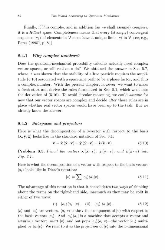
November 24, 2010 10:17 World Scientific Book - 9in x 6in main
82 The World According to Quantum Mechanics
Finally, if V is complex and in addition (as we shall assume) complete,
it is a Hilbert space. Completeness means that every (strongly) convergent
sequence |vk〉 of elements in V must have a unique limit |v〉 in V [see, e.g.,
Peres (1995), p. 81].
8.4.1 Why complex numbers?
Does the quantum-mechanical probability calculus actually need complex
vector spaces, or will real ones do? We obtained the answer in Sec. 5.7,
where it was shown that the stability of a free particle requires the ampli-
tude (5.16) associated with a spacetime path to be a phase factor, and thus
a complex number. With the present chapter, however, we want to make
a fresh start and derive the rules formulated in Sec. 5.1, which went into
the derivation of (5.16). To avoid circular reasoning, we could assume for
now that our vector spaces are complex and decide after those rules are in
place whether real vector spaces would have been up to the task. But we
already know the answer.
8.4.2 Subspaces and projectors
Here is what the decomposition of a 3-vector with respect to the basis
(x, y, z) looks like in the standard notation of Sec. 3.1:
v = x (x · v) + y (y · v) + z (z · v) . (8.10)
Problem 8.3. Pencil the vectors x (x · v), y (y · v), and z (z · v) into
Fig. 3.1.
Here is what the decomposition of a vector with respect to the basis vectors
|ai〉 looks like in Dirac’s notation:
|v〉 =∑
i
|ai〉〈ai|v〉 . (8.11)
The advantage of this notation is that it consolidates two ways of thinking
about the terms on the right-hand side, inasmuch as they may be split in
either of two ways:
(i) |ai〉〈ai| |v〉, (ii) |ai〉 〈ai|v〉 . (8.12)
|v〉 and |ai〉 are vectors. 〈ai|v〉 is the i-the component of |v〉 with respect to
the basis vectors |ai〉. And |ai〉〈ai| is a machine that accepts a vector and
returns a vector: insert |v〉, and out pops |ai〉〈ai|v〉—the vector |ai〉 multi-
plied by 〈ai|v〉. We refer to it as the projection of |v〉 into the 1-dimensional

November 24, 2010 10:17 World Scientific Book - 9in x 6in main
Why quantum mechanics? 83
subspace containing |ai〉, and we refer to an operator that projects into a
subspace as a projector. Think of (i) as what we do—projecting |v〉 into
the 1-dimensional subspace containing |ai〉—and of (ii) as what we get as
a result—the projection of |v〉 into this subspace.
A subspace is a vector space within a vector space. Specifically, U is a
subspace of V if and only if it satisfies the following condition: if |u〉 and
|v〉 are in U and a and b are numbers, then a|u〉+ b|v〉 is in U . If a subspace
U has a dimension that is (denumerably) infinite, we shall tacitly assume
that it is closed: every sequence of vectors in U that converges in V—i.e.,
that has as its limit a vector in V—also converges in U .
There is a one-to-one correspondence between subspaces and projectors.
If U is a subspace, so that there is in V a set of mutually orthogonal unit
vectors |b1〉, . . . , |bm〉 that allows every vector in U to be written as a linear
combination∑m
k=1 vk|bk〉, then there is a unique operator that projects into
U , namely,
P(U) =
m∑
k=1
|bk〉〈bk| . (8.13)
We say that U is spanned by the vectors |b1〉, . . . , |bm〉. While the projector
(8.13) is unique, the vectors that span U are not. If |c1〉, . . . , |cm〉 is a
different set of mutually orthogonal unit vectors that span U , then
m∑
k=1
|ck〉〈ck| =m∑
k=1
|bk〉〈bk| . (8.14)
Problem 8.4. If |v〉 ∈ U then P(U) |v〉 = |v〉.
Problem 8.5. P(U) P(U) = P(U).
If the vectors |ak〉 (k = 1, . . . , n) constitute a basis in V , then
I =n∑
k=1
|ak〉〈ak | (8.15)
is the identity operator, which projects every vector in V into V—a long-
winded way of saying that it does nothing.
Problem 8.6. The projector |v〉〈v| is invariant under the phase transfor-
mation |v〉 → eiα|v〉.

December 23, 2010 10:25 World Scientific Book - 9in x 6in main
84 The World According to Quantum Mechanics
Fig. 8.2 Two 2-dimensional subspaces of a 3-dimensional (real) vector space. Only in
the left diagram do the corresponding projectors commute.
8.4.3 Commuting and non-commuting projectors
Two operators A, B are said to commute if
AB = BA . (8.16)
This is the shorter way of saying that AB|v〉 = BA|v〉 for every vector |v〉.It is not hard to see that two projectors M and N commute if and only if
there is a basis |ai〉 such that
M =∑
some i
|ai〉〈ai| and N =∑
some k
|ak〉〈ak| . (8.17)
Consider the following example (Fig. 8.2):
M = |2〉〈2|+ |3〉〈3|, N = |1〉〈1|+ |3〉〈3| . (8.18)
Problem 8.7. (∗) The two projectors commute if there is a basis to which
the vectors |1〉, |2〉, |3〉 belong.
If |1〉 and |2〉 are not orthogonal (while the remaining pairs are), we have
MN = |2〉〈2|1〉〈1|+ |3〉〈3| , NM = |1〉〈1|2〉〈2|+ |3〉〈3| , (8.19)
that is, M and N do not commute. Figure 8.3 illustrates the respective
actions of MN and NM on a vector |v〉.Our next task is to translate the commutativity condition for projectors
into the language of subspaces. The following two definitions will help us
do this.

November 24, 2010 10:17 World Scientific Book - 9in x 6in main
Why quantum mechanics? 85
Fig. 8.3 The situation illustrated in Fig. 8.2 (right diagram) seen from above, looking
down the 3-axis. On the left, |v〉 is projected into M, then the resulting vector isprojected into N . On the right, |v〉 is projected into N , then the resulting vector isprojected into M.
• The orthocomplement A⊥ of a subspace A contains all vectors that are
orthogonal to all vectors in A.
• The span A∪B of two subspaces A and B is the smallest subspace that
contains both A and B.
Problem 8.8. A⊥ is a subspace.
Problem 8.9. The intersection A∩B of two subspaces, which contains all
vectors that are contained in both subspaces, is a subspace.
Problem 8.10. (A⊥)⊥ = A.
Problem 8.11. Convince yourself that A ⊂ B⊥ and B ⊂ A⊥ are equiva-
lent.
Figure 8.4 illustrates the relations that hold betweenM,N , their orthocom-
plements, and the intersections of all these just in case the corresponding
projectors M, N commute. We gather from it that
(M∩N ) ∪ (M∩N⊥) ∪ (M⊥ ∩ N ) ∪ (M⊥ ∩ N⊥) = V . (8.20)
This is the wanted expression of the commutativity condition for projectors
in terms of the corresponding subspaces. A quick check will confirm that
it is satisfied by the subspaces in the left half of Fig. 8.2: while M⊥ ∩ N⊥is empty,M⊥ ∩N is the subspace containing |1〉,M∩N⊥ is the subspace
containing |2〉, and M∩ N is the subspace containing |3〉. On the other
hand, Eq. (8.20) does not hold for the subspaces in the right half of Fig. 8.2:

November 24, 2010 10:17 World Scientific Book - 9in x 6in main
86 The World According to Quantum Mechanics
Fig. 8.4 The relations that hold between M, N , their orthocomplements, and theintersections of all these if the corresponding projectors can be written in terms of acommon basis, as in Eq. (8.17). The dots represent the basis vectors. The horizontalbracket associated with a subspace groups the 1-dimensional projectors that make upthe projector into that subspace. Above: neither of the subspaces M, N is contained inthe other. Below: M ⊂ N .
whileM∩N is the 1-dimensional subspace containing |3〉, the intersections
M∩N⊥, M⊥ ∩ N , andM⊥ ∩N⊥ are all empty.
8.5 Compatible and incompatible elementary tests
This brings us back to our central theme, the stability of matter. The sta-
bility of atoms requires an inequality of the form (4.18); the product of the
“uncertainties” associated with a relative position and the corresponding
relative momentum must have a positive lower limit. This makes it impos-
sible to simultaneously measure both quantities with arbitrary precision.
In other words, the stability of matter requires, via the stability of atoms,
that the two quantities be incompatible.
To arrive at a formal definition of compatibility, we consider two ele-
mentary tests. We first assume that one of the possible outcomes of the
second test (say, the positive outcome N ) is implied by one of the possible
outcomes of the first test (say, the positive outcome M): whenever the
outcomeM is obtained, a subsequent test of N is bound to yield a positive
result.
Problem 8.12. This is equivalent to M⊂ N .

November 24, 2010 10:17 World Scientific Book - 9in x 6in main
Why quantum mechanics? 87
Problem 8.13. If N represents the positive outcome of an elementary test,
N⊥ represents the negative outcome.
There are three possible combinations of outcomes: (i) M and N ,
(ii) M⊥ and N , (iii) M⊥ and N⊥. Requiring compatibility for the two
tests amounts to requiring that for each combination of outcomes there
should be an algorithm assigning to it a probability equal to 1. In other
words, the two tests are compatible if and only if there are three 1-dimen-
sional subspaces Li such that
(i) L1 ⊂M∩N : L1 assigns probability 1 to both M and N ,
(ii) L2 ⊂M⊥ ∩N : L2 assigns probability 1 to both M⊥ and N ,
(iii) L3 ⊂M⊥ ∩N⊥: L3 assigns probability 1 to both M⊥ and N⊥.
It is easy to see that these requirements are satisfied: M ⊂ N , therefore
L1 exists; N 6= M, so N contains a line orthogonal to M, therefore L2
exists; and because M ⊂ N implies N⊥ ⊂ M⊥ (Problem 8.11), therefore
L3 exists. Thus if either outcome of the first test implies either outcome of
the second test, the two tests are compatible.
If neither outcome of the first test implies either outcome of the sec-
ond test, then compatibility requires, in addition, the existence of a
1-dimensional subspace L4 such that
(iv) L4 ⊂M∩N⊥: L4 assigns probability 1 to both M and N⊥.
If these four requirements are satisfied, none of the intersections M∩ N ,
M∩N⊥,M⊥∩N , andM⊥∩N⊥ can be equal to ∅. Since these intersections
are mutually orthogonal, one can find a set of mutually orthogonal unit
vectors |ai〉 (i = 1, . . . , n) such that those with i = 1, . . . , j span M∩ N ,
those with i = j + 1, . . . , k spanM∩N⊥, those with i = k+ 1, . . . ,m span
M⊥ ∩ N , and those with i = m + 1, . . . , n span M⊥ ∩ N⊥. To establish
that the n vectors |ai〉 in fact constitute a basis, we assume the contrary.
We assume, in other words, that there is a 1-dimensional subspace L that
is orthogonal to each of those four intersections. But this is the same as
saying that there is a probability algorithm that assigns probability 0 to all
possible combinations of outcomes, and this is a reductio ad absurdum of
our assumption.
The bottom line: two elementary tests with respective positive outcomes
M and N are compatible if and only if Eq. (8.20) holds. (IfM⊂N , then
this equation holds with M∩N⊥ = ∅.)

December 23, 2010 10:25 World Scientific Book - 9in x 6in main
88 The World According to Quantum Mechanics
8.6 Noncontextuality
If the subspaces A and B represent measurement outcomes, what measure-
ment outcome is represented by the span A ∪ B?We begin with the following observations. Let p(A) and p(B) be the
respective probabilities of obtaining the outcomes represented by A and B.Because a 1-dimensional subspace that is contained in either A or B is
contained in A∪ B, we have that[p(A) = 1 or p(B) = 1
]=⇒ p(A ∪ B) = 1 . (8.21)
In words: if either A or B has probability 1, then A∪ B has probability 1.
Again, because a line orthogonal to both A and B is orthogonal to A ∪ B,we also have that
[p(A) = 0 and p(B) = 0
]=⇒ p(A ∪ B) = 0 . (8.22)
The implications (8.21) and (8.22) hold, in particular, if A and B represent
disjoint intervals A and B of a variable Q with a continuous range of values.
But note that a 1-dimensional subspace can be in A ∪ B without being
contained in either A or B. This means that the outcome A ∪ B can be
certain even if neither A nor B is certain. Obtaining the outcome A ∪ Btherefore does not imply that the value of Q is either A or B. A fortiori, it
does not imply that the value of Q is any smaller interval in either A or B,
let alone a definite number.
Next imagine two perfect—one hundred percent efficient—detectors
D(A) and D(B) monitoring the two intervals. If the probabilities p(A)and p(B) are both greater than 0 (and therefore less than 1), then it is not
certain that D(A) will click, and it is not certain that D(B) will click. Yet
if p(A ∪ B) = 1, then it is certain that either D(A) or D(B) will click.
What makes this certain?
The answer lies in the fact that quantum-mechanical probability assign-
ments are invariably made on the (tacit) assumption that a measurement
is successfully made; there is an outcome. For instance, if A and B are dis-
joint regions of space, and if a measurement has indicated the presence of
a particle in the union A∪B of these regions, then the tacit assumption is
that a subsequent position measurement made with two detectors monitor-
ing the respective regions A and B will yield an outcome—either detector
will click. So there is no mystery here, but the implication is that quantum
mechanics only gives us probabilities with which this or that outcome is
obtained in a successful measurement. It does not give us the probability

November 24, 2010 10:17 World Scientific Book - 9in x 6in main
Why quantum mechanics? 89
with which an attempted measurement will succeed. A fortiori, it is inca-
pable of formulating sufficient conditions for the success of a measurement
[Ulfbeck and Bohr (2001)].
Now consider the following two measurements. The first, M1, has three
possible outcomes: A, B, and C. The second, M2, has two: A ∪ B and C.We therefore have
p(A) + p(B) + p(C) = 1 as well as p(A∪ B) + p(C) = 1 . (8.23)
If, for instance, A, B, and C are disjoint regions of space, and if a particle
is certain to be found in the union of these regions, then M1 is certain to
find it in one of these three regions, while M2 is certain to find it in either
A ∪ B or C. It follows that
p(A ∪ B) = p(A) + p(B) . (8.24)
Or does it? Both measurements test for the possession of C, but whereas
M1 includes two additional tests, M2 only includes one. What gives us the
right to assume that the probability of a possible measurement outcome
is independent of what the other possible outcomes are? Equations (8.23)
hold in different experimental contexts. Is it legitimate to separate them
from their specific contexts so as to draw the conclusion (8.24)? In other
words, is it legitimate to assume noncontextuality?
Let us remember our objective. We are looking for a probability algo-
rithm that is capable of accommodating nontrivial probabilities and incom-
patible elementary tests. If common sense in the form of noncontextuality is
consistent with these requirements, we go for it. No need to make the world
stranger than it already is. By hindsight we know that Nature concurs.2
Problem 8.14. Projectors are said to be (mutually) orthogonal if the cor-
responding subspaces are. Show that the sum of two orthogonal projectors
is a projector.
Problem 8.15. If the orthogonal projectors A and B project into A and
B, respectively, the sum A + B projects into A ∪ B.
Problem 8.16. The projectors A and B corresponding to different out-
comes A and B of the same measurement are orthogonal.
2We also know that contextuality is an inescapable feature of situations in which prob-abilities are assigned either on the basis of past and future outcomes (Sec. 13.8.1) or tooutcomes of measurements performed on entangled systems (Sec. 13.4).

December 23, 2010 10:25 World Scientific Book - 9in x 6in main
90 The World According to Quantum Mechanics
8.7 The core postulates
We are now ready to assemble the core postulates of quantum mechanics.
The first was stated in Sec. 8.3:
Postulate 1. Measurement outcomes are represented by the projectors of
a vector space.
In Sec. 8.5 we concluded that two elementary testsM andN are compatible
if and only if Eq. (8.20) holds, and in Sec. 8.4.3 we found that this is the
case if and only if the corresponding projectors commute. Hence
Postulate 2. The outcomes of compatible elementary tests correspond to
commuting projectors.
From the previous section, finally, we derive the following:
Postulate 3. If A and B are orthogonal projectors, then the probability
of the outcome represented by A+ B is the sum of the probabilities of the
outcomes represented by A and B, respectively.
8.8 The trace rule
Postulates 1–3 are sufficient [Peres, 1995, p. 190] to prove Gleason’s theorem
[Gleason (1957); Pitowsky (1998); Cooke et al. (1985)], which holds for
vector spaces with at least three dimensions.3 The theorem states that
the probability of obtaining the outcome represented by the projector P is
given by
p(P) = Tr(WP) , (8.25)
where W is a unique operator, known as density operator, whose properties
will be listed in a moment. The trace of an operator X is defined by
Tr(X) =∑
i
〈ai|X|ai〉 , (8.26)
3More recently, the validity of Gleason’s theorem has been extended to include2-dimensional vector spaces [Fuchs (2001); Busch (2003); Caves et al. (2004)] by gener-alizing from the projector valued measures used in this book to positive operator valuedmeasures or POVMs [Peres, 1995, Sec. 9–5]. If outcomes are represented by positiveoperators, assigning probability 1 to one outcome no longer necessitates assigning prob-ability 0 to a different outcome of the same measurement. POVMs are thus suited fordealing with measurements that have overlapping outcomes, such as position measure-ments with detectors whose sensitive regions intersect.

December 23, 2010 10:25 World Scientific Book - 9in x 6in main
Why quantum mechanics? 91
where the vectors |ai〉 form a basis and the summation extends from i = 1
to the dimension of the system’s vector space. Think of 〈ai|X|ai〉 as the i-thcomponent of the vector X|ai〉 with respect to this basis. The definition of
the trace appears to be contingent on a basis, but actually this is not the
case. Let us insert a couple of identity operators I =∑
i |bi〉〈bi|:∑
i
〈ai|X|ai〉 =∑
i
〈ai |IXI|ai〉 =∑
i
∑
j
∑
k
〈ai|bj〉〈bj |X|bk〉〈bk|ai〉 .
Now we rearrange the complex factors on the right-hand side and take out
two identity operators:∑
i
∑
j
∑
k
〈bk|ai〉〈ai|bj〉〈bj |X|bk〉 =∑
j
∑
k
〈bk|bj〉〈bj |X|bk〉 =∑
k
〈bk|X|bk〉 .
Voila: the trace is independent of the basis that has been used in its defi-
nition.
Here is the promised list of properties of the density operator:
(i) W is linear : W(α|a〉+ β|b〉
)= α W|a〉+ β W|b〉.
(ii) W is self-adjoint : 〈a|W|b〉 = 〈b|W|a〉∗.(iii) W is positive: 〈a|W|a〉 ≥ 0.
(iv) Tr(W) = 1.
(v) W2 ≤ W.
Let us try to understand why W has these properties.
Problem 8.17. If P is a 1-dimensional projector |v〉〈v|, the trace
rule (8.25) reduces to p(P) = 〈v|W|v〉.
The fact that W is self-adjoint ensures that the probability 〈v|W|v〉 is a
real number. (What could be the meaning of a complex probability?)
The positivity of W ensures that 〈v|W|v〉 does not come out negative.
(What could be the meaning of a negative probability?)
The outcomes of a maximal test (also known as a complete measure-
ment) are represented by a complete system of (mutually orthogonal)
1-dimensional projectors |ak〉〈ak| (k = 1, . . . , n). Tr(W) = 1 ensures that
the corresponding probabilities 〈ai|W|ai〉 add up to 1. Together with the
positivity of W, this ensures that no probability comes out greater than 1.
(What could be the meaning of a probability greater than 1?)
The last property covers two possibilities, W2 = W and W2 < W.
These will be discussed after a short mathematical digression.

November 24, 2010 10:17 World Scientific Book - 9in x 6in main
92 The World According to Quantum Mechanics
8.9 Self-adjoint operators and the spectral theorem
In what follows we take the liberty of writing |Ab〉 instead of A|b〉 when
referring to the vector returned by A upon insertion of |b〉.If A is a linear operator (like W above), there exists a linear operator
A†, called the adjoint of A, such that 〈a|Ab〉 = 〈A†a|b〉 for every pair of
vectors |a〉, |b〉.
Problem 8.18. 〈a|Ab〉 = 〈b|A†a〉∗.
Problem 8.19. Show that (i) (A†)† = A and (ii) (AB)† = B†A†.
If (i) A is linear, (ii) |a〉 is a vector, and (iii) α is a complex number such
that A|a〉 = α|a〉, then |a〉 is an eigenvector of A and α is the corresponding
eigenvalue.
Problem 8.20. A projector has exactly two eigenvalues, namely. . . .
Saying that A is self-adjoint is the same as saying that A† = A. Self-
adjoint operators have two important properties. For one, their eigenvalues
are real, as we gather from the following equations:
α〈a|a〉 = 〈a|Aa〉 = 〈Aa|a〉 = α∗〈a|a〉 . (8.27)
For another, the eigenvectors of a self-adjoint operator that correspond
to different eigenvalues α1 6= α2 are orthogonal, as we gather from these
equations:
0 = 〈a1|Aa2〉 − 〈Aa1|a2〉 = (α2 − α1)〈a1|a2〉 . (8.28)
Problem 8.21. If a linear operator A has m > 1 linearly independent
eigenvectors with the same eigenvalue, then the eigenvectors of A corre-
sponding to this eigenvalue form an m-dimensional subspace.
For every self-adjoint operator A, it is possible to construct a basis made up
entirely of eigenvectors of A [see, for example, Marchildon, 2002, Sec. 2.5].
Suppose that the vectors |ai〉 constitute such a basis, and that the corre-
sponding eigenvalues are αi. Define the operator A′ =∑
i αi |ai〉〈ai| and
insert into it the generic vector |v〉 = ∑j vj |aj〉:
A′|v〉 =∑
i
∑
j
αivj |ai〉〈ai|aj〉 =∑
i
αivi|ai〉 . (8.29)
We would get the same result if we inserted |v〉 into A. But if two operators
act in the same way on every vector, they are identical: A′ = A. Hence

January 10, 2011 12:20 World Scientific Book - 9in x 6in main
Why quantum mechanics? 93
the spectral theorem, which says that every self-adjoint operator A has a
spectral decomposition
A =∑
i
αi |ai〉〈ai| . (8.30)
The eigenvalues αi form the spectrum of A.
Problem 8.22. Write down the spectral decomposition of a projector P.
Problem 8.23. (∗) A self-adjoint operator satisfying A2 = A is a projec-
tor.
Problem 8.24. The trace of a projector is the dimension of the subspace
into which it projects.
8.10 Pure states and mixed states
If the density operator is idempotent (i.e., W2 = W), it is a projector,
and since the trace of W equals unity, it projects into a 1-dimensional
subspace. Since we began by upgrading from a point in a phase space to a
line (or ray) in a vector space, we are not surprised by this result. In this
case W = |w〉〈w| is called a pure state, |w〉 is referred to as a state vector
(which is unique up to a phase factor), and the trace rule simplifies to
p(P) = 〈w|P|w〉 . (8.31)
If in addition P = |v〉〈v|, the trace rule boils down to the Born rule,
p(P) = 〈w|v〉〈v|w〉 = |〈v|w〉|2. (8.32)
If W2 < W, which means that 〈a|W2|a〉 < 〈a|W|a〉 for every vector |a〉,then W is called a mixed state or mixture. What do we make of this
possibility? Given a spectral decomposition of W, the inequality W2 < W
takes the form∑
k
α2k |ak〉〈ak| <
∑
k
αk |ak〉〈ak| . (8.33)
Problem 8.25. (∗) For all eigenvalues αk of a mixture, 0 < αk < 1.
Problem 8.26. (∗) ∑k αk = 1.

January 10, 2011 12:20 World Scientific Book - 9in x 6in main
94 The World According to Quantum Mechanics
The eigenvalues of a mixed state thus have all the properties one ex-
pects from nontrivial probabilities associated with mutually exclusive and
jointly exhaustive possibilities: they are real, they are greater than 0,
they are less than 1, and they add up to 1. The obvious conclusion is
that mixed states define probability distributions over probability distri-
butions. They add a second layer of uncertainty to that inherent in pure
states. There are situations in which this additional uncertainty is sub-
jective in the same sense in which probability distributions over a clas-
sical phase space are subjective: the uncertainty arises from a lack of
knowledge of relevant facts. But there are also situations in which the
additional uncertainty is due to the nonexistence of relevant facts. In
these situations it represents an additional objective fuzziness, over and
above that associated with the individual projectors |ak〉〈ak| in Eq. (8.33).
We will encounter some examples of this kind of uncertainty in later
chapters.
8.11 How probabilities depend on measurement outcomes
It bears repetition: quantum mechanics serves to assign probabilities to
possible measurement outcomes on the basis of actual outcomes. What we
have learned so far in this chapter is (i) that the probabilities of possible
measurement outcomes are encoded in a density operator and (ii) how they
can be extracted from it. Our next order of business is to find out how the
density operator is determined by actual outcomes.
Suppose that W1 is the density operator appropriate for assigning prob-
abilities to the possible outcomes of any measurement that may be made
at the time t1. And suppose that a measurement M is made at t1, and
that the outcome obtained is represented by the projector P. What is the
density operator W2 appropriate for assigning probabilities to the possible
outcomes of whichever measurement may be made next, at t2 > t1?
As is customary in discussions of this kind, we focus on repeatable
measurements. If a physical system is subjected to two consecutive identical
measurements, and if the second measurement invariably yields the same
outcome as the first, we call these measurements repeatable.4
4This definition departs from the standard definition in that it allows W2 to be inde-pendent of the time interval between the two measurements. (The standard definitionassumes that the second measurement is performed “immediately” after the first.)

November 24, 2010 10:17 World Scientific Book - 9in x 6in main
Why quantum mechanics? 95
Let us put together the relevant information at hand:
(i) W2 is constructed out of W1 and P.
(ii) Tr(W2P`) = 0, where P` is any possible outcome of M other than P.
(iii) W2 is self-adjoint.
(iv) Tr(W2P) = 1.
Problem 8.27. WP is self-adjoint if and only if W and P commute.
The first two conditions are satisfied by W2 = W1P, W2 = PW1, and
W2 = PW1P, but only the last of these candidates satisfies the third
condition in case W1 and P fail to commute. To satisfy the final condition
as well, all we have to do is divide by Tr(W1P) = Tr(PW1) = Tr(PW1P).
Thus,
W2 =PW1P
Tr(W1P). (8.34)
Now suppose that M is a maximal test, and that P = |w〉〈w|. Then
W2 =|w〉〈w|W1|w〉〈w|Tr(W1|w〉〈w|)
= |w〉 〈w|W1|w〉〈w|W1|w〉
〈w| = |w〉〈w| . (8.35)
Lo and behold, if we update the density operator to take into account the
outcome of a maximal test, it turns into the very projector that represents
this outcome. Observe that in this case W2 is independent of W1.
8.12 How probabilities depend on the times of
measurements
We now relax the condition of repeatability and require only that mea-
surements be verifiable. A measurement M1, performed at the time t1, is
verifiable if it is possible to confirm its outcome by a measurement M2 per-
formed at the time t2 > t1. If M1 is repeatable, then it can be verified by
simply repeating it. Otherwise the verification requires (i) the performance
of a different measurement and (ii) the existence of a one-to-one correspon-
dence between the possible outcomes of M1 and those of M2. The second
requirement makes it possible to infer the outcome of M1 from the outcome
of M2.
If the two measurements are maximal tests, then there are two bases,
one made up of the vectors |ai〉, the other made up of the vectors |bk〉, such
that the projectors |ai〉〈ai| represent the possible outcomes of M1 and the

November 24, 2010 10:17 World Scientific Book - 9in x 6in main
96 The World According to Quantum Mechanics
projectors |bk〉〈bk| represent the possible outcomes of M2. The two bases
are related by some transformation
|ak〉 −→ |bk〉 = U|ak〉 . (8.36)
8.12.1 Unitary operators
What do we know about the operator U? To begin with, in the absence of
time-dependent influences acting on the measured system (and especially if
the system is closed, which for the moment we will assume), U may depend
on the time difference t2 − t1 but not on t1 or t2 individually.
Suppose, next, that at t1 the generic outcome |w〉〈w| has been obtained.
Since the probabilities of the possible outcomes at t2 add up to unity, we
must have that∑
k
|〈bk|U(t2 − t1)|w〉|2 = 1 . (8.37)
Omitting the time dependence of U, we can rewrite the left-hand side of
Eq. (8.37) in a number of ways:∑
k
|〈bk|U|w〉|2 =∑
k
〈Uw|bk〉〈bk|Uw〉 = 〈Uw|Uw〉 = 〈w|U†U|w〉 ,
and it goes without saying to you should be checking the validity of each
equality. Equation (8.37) thus implies that
U†U = I . (8.38)
This makes U a unitary operator. By definition of the inverse operator
U−1, which undoes the action of U, we also have that
U−1U = I . (8.39)
A unitary operator may therefore also be characterized by saying that its
inverse equals its adjoint:
U−1 = U†. (8.40)
Problem 8.28. (∗) The scalar product is invariant under unitary trans-
formations: 〈Uw|Uv〉 = 〈w|v〉.
Problem 8.29. (∗) The eigenvalues of unitary operators are phase factors.
Problem 8.30. (∗) If U|u〉 = λ|u〉 then U†|u〉 = λ−1|u〉.

November 24, 2010 10:17 World Scientific Book - 9in x 6in main
Why quantum mechanics? 97
Problem 8.31. (∗) Eigenvectors of a unitary operator corresponding to
distinct eigenvalues are orthogonal.
Problem 8.32.[∑K
k=1 λk |ak〉〈ak|]n
=∑K
k=1 λnk |ak〉〈ak|.
As you will recall, for every self-adjoint operator A one can construct a
basis made up of eigenvectors of A. The same is true for every unitary
operator U. The spectral decomposition of a unitary operator has the
form
U =∑
k
eiαk |ak〉〈ak| . (8.41)
Let A be self-adjoint. If we define eiA via the Taylor series of the expo-
nential function and use the spectral decomposition of A, we find that the
eigenvectors of eiA are the same as those of A. And if the corresponding
eigenvalues of A are λk, then the corresponding eigenvalues of U are the
phase factors eiλk :
eiA =
∞∑
n=0
(iA)n
n!
=∞∑
n=0
in
n!
[K∑
k=1
λk|ak〉〈ak|]n
=∞∑
n=0
in
n!
K∑
k=1
λnk |ak〉〈ak|
=
∞∑
n=0
K∑
k=1
(iλk)n
n!|ak〉〈ak |
=
K∑
k=1
eiλk |ak〉〈ak| . (8.42)
Thus every unitary operator U can be cast into the form eiA, where A is
self-adjoint.
There’s something else we know about U(t2− t1). Since (t2 − t1) is the
amount of time we wait before performing the second measurement, and
since waiting from t1 to t2 is the same as waiting from t1 to t′ < t2 and
then waiting some more, from t′ to t2, we have that
U(t2 − t1) = U(t2 − t′) U(t′ − t1) , (8.43)

November 24, 2010 10:17 World Scientific Book - 9in x 6in main
98 The World According to Quantum Mechanics
and thus
eiA(t2−t1) = eiA(t2−t′) eiA(t′−t1) . (8.44)
Since we also have that
eiA(t2−t′) eiA(t′−t1) = ei[A(t2−t′)+A(t′−t1)] ,
we find that A depends linearly on its argument:
A(t2 − t′) + A(t′ − t1) = A((t2 − t′) + (t′ − t1)
)= A(t2 − t1) .
This allows us to introduce a self-adjoint operator H, known as the Hamil-
ton operator or simply the Hamiltonian, such that
U(∆t) = e−(i/~) H∆t. (8.45)
The negative sign is again a convention. The division by ~ ensures that the
eigenvalues of H are measured in energy units. For infinitesimal dt we thus
have that
U(dt) = I− i
~H dt . (8.46)
If we apply both sides to a vector |v〉 and use |v(t+ dt)〉 = U(dt)|v(t)〉, we
obtain
|v(t+ dt)〉 − |v(t)〉 = − i~H|v(t)〉 dt , (8.47)
and thus
d|v〉dt
= − i~H|v〉 . (8.48)
If the experimental conditions are time-dependent, U depends on t in ad-
dition to its dependence on dt. This additional dependence goes into H.
If we use vector components vj = 〈aj |v〉 and operator components
Hjk = 〈aj |H|ak〉, we can cast Eq. (8.48) into the form
i~dvj
dt=
K∑
k=1
Hjkvk (for j = 1, . . . ,K) . (8.49)

November 24, 2010 10:17 World Scientific Book - 9in x 6in main
Why quantum mechanics? 99
8.12.2 Continuous variables
When dealing with a continuous variable—say, the position of a particle in
one spatial dimension—it is customary to introduce a non-denumerably in-
finite basis of “improper” vectors |x〉. With respect to such a basis, a generic
vector |v〉 has the components v(x) = 〈x|v〉, and the Hamiltonian has the
components H(x, x′) = 〈x|H|x′〉. In place of the sum |v〉 =∑
k |ak〉〈ak|v〉we then have the integral
|v〉 =
∫ +∞
−∞dx |x〉〈x|v〉 , (8.50)
and in place of Eq. (8.49) we have
i~∂v(x, t)
∂t=
∫ +∞
−∞dx′H(x, x′) v(x′, t) . (8.51)
In addition, the orthonormality condition 〈ai|ak〉 = δik (Eq. 8.9) gets re-
placed by 〈x|x′〉 = δ(x− x′). The delta distribution δ(x− x′) is defined by
requiring that for any continuous function f(x),
∫ x2
x1
dx δ(x − x0)f(x) = f(x0) , (8.52)
where x1 < x0 < x2.5
As it stands, however, Eq. (8.51) is inconsistent with the special theory
of relativity (Chap. 6). The problem is that the left-hand side depends
on the time rate of change of v for a single value of x, while the right-
hand side depends on the simultaneous value of v for every value of x. The
instantaneous action at a distance implied by this dependence is not possible
in a relativistic world. The remedy is to include a delta distribution in the
definition of the Hamiltonian: H(x, x′) = δ(x − x′) H. Because H(x, x′)may depend on how v(x, t) changes locally, across infinitesimal intervals, H
may contain differential operators with respect to x. Hence the hat: H is
still an operator, albeit one acting on the function v(x, t) rather than one
acting on the vector |v〉. Equation (8.51) now takes the acceptable form
i~∂v(x, t)
∂t= H v(x, t) . (8.53)
Problem 8.33. Write down the Hamiltonians for Eq. (4.4) and Eq. (7.21).
5For further discussion of the delta distribution see Marchildon (2002, Sec. 5.9.1) orPeres (1995, Sec. 4.7).

December 23, 2010 10:25 World Scientific Book - 9in x 6in main
100 The World According to Quantum Mechanics
8.13 The rules of the game derived at last
The origin of the two rules formulated in Sec. 5.1, one of which led us to the
Schrodinger equation via the Feynman route, is now readily understood.
Suppose that a maximal test performed at the time t1 yields the out-
come |u〉〈u|, or u for short, and that we want to calculate the probability
with which a maximal test performed at the time t2 > t1 yields the outcome
w. Assume that at some intermediate time t another maximal test is made,
and that its possible outcomes are vi (i = 1, . . . , n). Because a maximal
test “prepares from scratch,” as we have seen in Sec. 8.11, the joint proba-
bility p(w, vi|u) with which the intermediate and final tests yield vi and w,
respectively, given the initial outcome u, is the product of two probabili-
ties: the probability p(vi|u) of vi given u, and the probability p(w|vi) of wgiven vi. By Born’s rule (8.32), this is
p(w, vi|u) = |〈w|vi〉〈vi|u〉|2. (8.54)
The probability of w given u, regardless of the intermediate outcome, is
given by Rule A: first take the absolute squares of the amplitudes Ai =
〈w|vi〉〈vi|u〉, then add the results:
pA(w|u) =∑
i
p(w, vi|u) =∑
i
|〈w|vi〉〈vi|u〉|2. (8.55)
If no intermediate measurement is made, we have pB(w|u) = |〈w|u〉|2, andif we insert the identity operator I =
∑
i |vi〉〈vi|, we obtain
pB(w|u) =∣∣∣∣∣
∑
i
〈w|vi〉〈vi|u〉∣∣∣∣∣
2
. (8.56)
In other words, first add the amplitudes Ai, then take the absolute square
of the result.

November 24, 2010 10:17 World Scientific Book - 9in x 6in main
Chapter 9
The classical forces: Effects
9.1 The principle of “least” action
Let us return to the propagator for a stable scalar particle (Eq. 7.13):
〈rB , tB |rA, tA〉 =∫
DC e(i/~)∫
CdS. (9.1)
The path integral sums contributions from all timelike paths that start at
rA at the time tA and end at rB at the time tB . Why only timelike paths?
Actually there is no law that excludes other paths. Such paths exclude
themselves, as it were.
To see how, consider again a free particle, and suppose that C has a
spacelike segment ∆C. In this case we have that ds2 < 0 for all infinitesimal
segments dC that make up ∆C. The integral∫
∆C ds is therefore imaginary.
This means that the amplitude e(i/~)∫
Cds contains the factor e(i/~)
∫
∆Cds,
which has a real exponent. This factor (and hence the amplitude) either
blows up or falls off exponentially with (roughly) the distance between the
endpoints of ∆C. If the propagator is to yield finite probabilities, it must
fall off exponentially. As a result, spacelike (“superluminal”) propagation
is exponentially suppressed. It is not impossible, but it is very unlikely,
except over very short distances.
What then is the probability of finding that the particle has traveled
from spacetime point (rA, tA) to spacetime point (rB , tB) via a specific path
C0? Since the magnitude of Z[C] = e(i/~)∫
Cds is the same for all paths from
(rA, tA) to (rB , tB), this probability seems to be the same for all paths. It
is, however, strictly impossible to ascertain, by any kind of measurement or
sequence of measurements, that a particle has traveled via a definite path.
We obtain a more useful answer if we make the half realistic assumption
that what can be ascertained is whether a particle has traveled from (rA, tA)
to (rB , tB) inside a narrow bundle of paths.
101

November 24, 2010 10:17 World Scientific Book - 9in x 6in main
102 The World According to Quantum Mechanics
Imagine a narrow “tube” T filled with paths from (rA, tA) to (rB , tB).
The probability of finding that the particle has traveled from (rA, tA) to
(rB , tB) inside T is (formally) given by the absolute square of the path
integral
IT =
∫
TDC e(i/~)S[C], (9.2)
which sums over the paths from (rA, tA) to (rB , tB) that are contained
in T . We shall assume that there is a single path from (rA, tA) to (rB , tB)
for which the action S[C] is stationary : it does not change under small
variations of this path.1 Since the action differential dS defines a spacetime
geometry (Sec. 7.1), this is the same as assuming that there is a single
geodesic G connecting (rA, tA) with (rB , tB). (A geodesic is a path G that
is either longer or shorter than all paths that have the same endpoints as Gand lie in a sufficiently small neighborhood of G.)
If we further assume that G lies inside T , then there is a neighborhood
N of G inside T such that the phases S[C]/~ of the paths contained in Nare almost equal to that of G. As a result, the sum of the corresponding
phase factors e(i/~)S[C] is of considerable magnitude, and so is the path
integral IT . This is illustrated by the almost straight chain of arrows in
Fig. 9.1, which represent the almost equal phase factors contributed by the
paths inside N .
If G does not lie inside T , and if the differences between the phases of
the paths contained in T are sufficiently large, the magnitude of the sum
of the corresponding phase factors e(i/~)S[C] will be minute by comparison.
This is illustrated by the coiled chain of arrows in Fig. 9.1.
How large is “sufficiently large”?
For a free and stable particle, whose action is given by S[C] = −∫mc2ds
(Eq. 7.5), “sufficiently large” translates to “sufficiently large mass.” In
the limit m → ∞, the only paths that contribute to IT are those in the
infinitesimal neighborhood of G.For a stable particle moving under the kind of influence that is repre-
sented by the potentials V and A (Eq. 7.8), the relevant theoretical limit
is the classical limit ~→ 0. In this limit, it is safe to assume that a particle
traveling from (rA, tA) to (rB , tB) travels via G, as classical physics asserts.
A classical particle follows a geodesic of the geometry defined by the action
differential dS. If dS is given by Eq. (7.8), the resulting differential geom-
etry is of a type known as Finsler geometry (Antonelli et al., 1993; Rund,
1969).1This assumption ensures that a unique path is obtained in the classical limit.

November 24, 2010 10:17 World Scientific Book - 9in x 6in main
The classical forces: Effects 103
Fig. 9.1 The almost straight chain of arrows represents the almost equal phase factorscontributed by the paths inside a narrow bundle that contains the geodesic G. The coiledchain of arrows represents the phase factors contributed by the paths inside a narrowbundle that does not contain G.
If we are dealing with a system that has N degrees of freedom, the
configuration of the system is equivalent to a point in an N -dimensional
configuration space, and the propagator sums contributions from all paths
in the system’sN+1-dimensional configuration spacetimeM that lead from
a point P1 to a point P2:
〈P2, t2|P1, t1〉 =∫
DC e(i/~)S[C]. (9.3)
(P1 specifies the values of all degrees of freedom at the time t1, and P2 does
the same for t2.) In the classical limit, this system too follows a geodesic

November 24, 2010 10:17 World Scientific Book - 9in x 6in main
104 The World According to Quantum Mechanics
of the geometry defined by dS—i.e., a path G in M whose action S[G]is stationary under small variations of G. Although G does not have to
minimize the action (it might maximize it instead), the principle that lies
at the roots of classical physics is often referred to as the “principle of least
action.”
9.2 Geodesic equations for flat spacetime
Let us now take a spacetime path C leading from spacetime point A to
spacetime point B and vary it in such a way that every point (r, t) of Cgets displaced to a point (r + δr, t + δt) except for the fixed end points:
δt = 0 and δr = 0 at both A and B.
In what follows we must take care to distinguish between the duration
dt associated with an infinitesimal path segment dC and the variation δt of
the time component of a point on C. If we write t1 and t2 for the endpoints
of dt, it is easy to see that the variation of C changes dt into dt+ d δt:
dt = t2−t1 → (t2+δt2)−(t1+δt1) = (t2−t1)+(δt2−δt1) = dt+d δt . (9.4)
By the same token, dr→ dr + d δr. The corresponding variation of dS is
dS(t, r, dt, dr) → dS(t+ δt, r + δr, dt+ d δt, dr + d δr) . (9.5)
Expanding the variation of dS to first order in the differentials and using
the following shorthand notations,
∂ dS
∂r· δr =
∂ dS
∂xδx+
∂ dS
∂yδy +
∂ dS
∂zδz ,
∂ dS
∂ dr· d δr =
∂ dS
∂ dxd δx+
∂ dS
∂ dyd δy +
∂ dS
∂ dzd δz , (9.6)
we obtain
dS(t, r, dt, dr) +∂ dS
∂tδt+
∂ dS
∂r· δr +
∂ dS
∂ dtd δt+
∂ dS
∂ dr· d δr . (9.7)
The difference between the varied and the original path elements, accord-
ingly, is
δdS =∂ dS
∂tδt+
∂ dS
∂r· δr +
∂ dS
∂ dtd δt+
∂ dS
∂ dr· d δr . (9.8)

November 24, 2010 10:17 World Scientific Book - 9in x 6in main
The classical forces: Effects 105
We now use the product rule (Eq. 3.13),
d
[∂ dS
∂ dtδt
]
=
[
d∂ dS
∂ dt
]
δt+∂ dS
∂ dtd δt , (9.9)
d
[∂ dS
∂ dr· δr]
=
[
d∂ dS
∂ dr
]
· δr +∂ dS
∂ dr· d δr , (9.10)
to replace the partial derivatives with respect to dt and dr:
δ dS =∂ dS
∂tδt+
∂ dS
∂r· δr + d
[∂ dS
∂ dtδt
]
−[
d∂ dS
∂ dt
]
δt
+ d
[∂ dS
∂ dr· δr]
−[
d∂ dS
∂ dr
]
· δr . (9.11)
Integrating over C, we obtain the variation of S[C]:
δS[C] =
∫
C
[(∂ dS
∂t− d ∂ dS
∂ dt
)
δt+
(∂ dS
∂r− d ∂ dS
∂ dr
)
· δr]
+
∫
Cd
[∂ dS
∂ dtδt+
∂ dS
∂ dr· δr]
. (9.12)
The second integral only depends on the endpoints of C, at which δt = 0 and
δr = 0. It therefore vanishes. If C is a geodesic, the action is stationary, so
that δS[C] vanishes, too. The first integral then vanishes as well. Moreover,
since this vanishes for all possible variations δt and δr along C, its integrand
itself vanishes. The bottom line is that the geodesics defined by dS satisfy
the geodesic equations
∂ dS
∂t= d
∂ dS
∂ dt, (9.13)
∂ dS
∂r= d
∂ dS
∂ dr. (9.14)
9.3 Energy and momentum
If we look at these equations, what jumps out at us right away is that if
dS has no explicit time-dependence (i.e., ∂ dS/∂t = 0), then the system’s
energy
EDef= −∂ dS
∂ dt(9.15)
is constant along geodesics—the paths that classical systems follow in their
configuration spacetimes. (We’ll get to the reason for the negative sign in

November 24, 2010 10:17 World Scientific Book - 9in x 6in main
106 The World According to Quantum Mechanics
a moment.) Likewise, if dS has no explicit dependence on the components
of r (i.e., ∂ dS/∂r = 0), then the system’s momentum
pDef=
∂ dS
∂ dr(9.16)
is constant along geodesics.
E tells us how much the projection dt of a segment dC of a path C onto
the time axis contributes to S[C], and p tells us how much the projection dr
of dC onto space—the hyperplane spanned by the space axes—contributes
to S[C]. If dS has no explicit time dependence, then equal intervals of
the time axis make equal contributions to S[C]: they are physically equiv-
alent : they represent equal durations. If dS has no explicit dependence on
any space coordinate, then equal intervals of the space axes make equal
contributions to S[C]: they are physically equivalent : they represent equal
distances.
The take-home message here is that energy is defined as the physical
quantity whose constancy warrants the physical equivalence of equal time
intervals, often called the “homogeneity of time,” while momentum is de-
fined as the physical quantity whose constancy warrants the physical equiv-
alence of equal space intervals, often called the “homogeneity of space.” If
energy and/or momentum is/are not conserved, so that equal intervals of
the time and/or space axis are not physically equivalent, the reason could
be either that the system is not freely moving—an external influence ren-
ders quantitatively equal intervals physically inequivalent—or that we are
using the wrong coordinates: coordinates that give rise to fictitious forces.
More can be discovered by differentiating Eq. (7.7) with respect to u.
For the left-hand side we obtain
d(dS)
du=
∂ dS
∂(u dt)
∂(u dt)
∂u+
∂ dS
∂(u dr)· ∂(u dr)
∂u=
∂ dS
∂(u dt)dt+
∂ dS
∂(u dr)· dr ,
while the right-hand side comes out equal to dS. If we now set u = 1 and
use definitions (9.15) and (9.16), we arrive at
−E dt+ p · dr = dS . (9.17)
Since dS is a 4-scalar, the left-hand side, too, has to be a 4-scalar. Fur-
thermore, since (c dt, dr) are the components of a 4-vector, the left-hand
side has to be the scalar product of two 4-vectors. The second 4-vector,
(E/c,p), is the particle’s energy–momentum or 4-momentum. The reason
why we defined E and p with opposite signs should now be clear.

November 24, 2010 10:17 World Scientific Book - 9in x 6in main
The classical forces: Effects 107
Problem 9.1. If ds =√
dt2 − dr · dr/c2, then
∂ ds
∂ dt=
1√
1− v2/c2and
∂ ds
∂ dr= − v/c2
√
1− v2/c2.
Plugging the action differential of Sec. 7.2,
dS = −mc2 ds− qV (t, r) dt+q
cA(t, r) · dr , (9.18)
into the definitions (9.15) and (9.16) of E and p, we find that
E =mc2
√
1− v2/c2+ qV , (9.19)
p =mv
√
1− v2/c2+q
cA . (9.20)
Both E and p are thus made up of a kinetic part and a potential part. The
kinetic parts EK and pK are those containing the root; the potential parts
are EP = qV and pP = (q/c)A.
Problem 9.2. The kinetic parts of (9.19) and (9.20) satisfy the relation
E2 − p2c2 = m2c4 . (9.21)
Problem 9.3. Use the Taylor series to show that
(
1− v2
c2
)−1/2
= 1 +1
2
v2
c2+
3
8
v4
c4+ · · · . (9.22)
Expanding the kinetic parts of (9.19) and (9.20) and dropping all terms
having c in the denominator, we obtain the non-relativistic expressions
E = mc2 +m
2v2, p = mv . (9.23)
Because the term mc2 amounts to the presence of a (physically irrelevant)
constant potential, it can be dropped.
9.4 Vector analysis: Some basic concepts
We already encountered the gradient of a function f(x, y, z)—a vector
∂f/∂r whose components are
∂f
∂x,∂f
∂y,∂f
∂z. (9.24)

November 24, 2010 10:17 World Scientific Book - 9in x 6in main
108 The World According to Quantum Mechanics
The “vector” ∂/∂r, whose components are the differential operators
∂
∂x,∂
∂y,∂
∂z, (9.25)
is useful in a variety of ways. The product
dr · ∂∂r
, (9.26)
for example, is a machine that accepts a function f(x, y, z) and returns
the difference between the respective values of f at the points (x + dx,
y + dy, z + dx) and (x, y, z):
df =∂f
∂xdx+
∂f
∂ydy +
∂f
∂zdz . (9.27)
Problem 9.4. The integral of a gradient along a curve C only depends on
the endpoints of C.
9.4.1 Curl and Stokes’s theorem
Another useful application of the operator ∂/∂r is the curl of a vector field
A(x, y, z), abbreviated to curl A and defined by
∂
∂r× A =
(∂Az
∂y− ∂Ay
∂z
)
x +
(∂Ax
∂z− ∂Az
∂x
)
y +
(∂Ay
∂x− ∂Ax
∂y
)
z .
(9.28)
To uncover its significance, we calculate the circulation of A along a closed
curve C. This is given by the line integral∮
A · dr along C. (A line integral
along a closed curve is also called a loop integral.)
Let’s start with the boundary of an infinitesimal rectangle with cor-
ners A = (0,−dy/2,−dz/2), B = (0, dy/2,−dz/2), C = (0, dy/2, dz/2),
and D = (0,−dy/2, dz/2). The contributions from the four sides are,
respectively,
AB : +Ay(0, 0,−dz/2) dy = +
(
Ay(0, 0, 0)− ∂Ay
∂z
dz
2
)
dy ,
BC : +Az(0,+dy/2, 0) dz = +
(
Az(0, 0, 0) +∂Az
∂y
dy
2
)
dz ,
CD : −Ay(0, 0,+dz/2) dy = −(
Ay(0, 0, 0) +∂Ay
∂z
dz
2
)
dy ,
DA : −Az(0,−dy/2, 0) dz = −(
Az(0, 0, 0)− ∂Az
∂y
dy
2
)
dz . (9.29)

November 24, 2010 10:17 World Scientific Book - 9in x 6in main
The classical forces: Effects 109
Fig. 9.2 Illustration of Stokes’s theorem.
They add up to(∂Az
∂y− ∂Ay
∂z
)
dy dz =
(∂
∂r× A
)
x
dy dz . (9.30)
The next step is to represent our infinitesimal rectangle by a vector dΣ per-
pendicular to the rectangle and having a magnitude equal to the rectangle’s
area dy dz. This leaves us with two possible orientations. By convention,
the orientation of dΣ is determined by another right hand rule: stick out
your right thumb and curve the other fingers of your right hand. If the
curved fingers indicate the direction of integration along the rectangle’s
boundary, the thumb indicates the orientation of dΣ.
Thus we may write the circulation (9.30) as curl A · dΣ. Now we take
some finite surface Σ (Fig. 9.2) and divide it into infinitesimal rectangles like
the one just discussed. (We cannot divide any old surface into finite rect-
angles, but keeping in mind the limit indicated by the word “infinitesimal,”
we can divide it into infinitesimal rectangles.) The sum of the circulations
of all those infinitesimal rectangles is given by the surface integral∫
Σ
curl A · dΣ .
A glance at Fig. 9.2 informs us that the adjacent sides of neighboring rect-
angles contribute with opposite signs, since they are integrated over in
opposite directions. Their contributions to the surface integral thus can-
cel out and only the contributions from the boundary ∂Σ of Σ survive.

November 24, 2010 10:17 World Scientific Book - 9in x 6in main
110 The World According to Quantum Mechanics
The bottom line:∫
Σ
∂
∂r× A · dΣ =
∮
∂Σ
A · dr . (9.31)
This is Stokes’s theorem.
Problem 9.5. The loop integral of a gradient vanishes.
Hence by Stokes’s theorem,∫
Σ
(∂
∂r× ∂f
∂r
)
· dΣ = 0 . (9.32)
Because this holds for every surface Σ, the curl of a gradient vanishes
identically:
∂
∂r× ∂f
∂r≡ 0 . (9.33)
9.4.2 Divergence and Gauss’s theorem
Yet another useful application of the operator ∂/∂r is the divergence of a
vector field B(x, y, z), abbreviated to div B and defined by
∂
∂r·B =
∂Bx
∂x+∂By
∂y+∂Bz
∂z. (9.34)
To uncover its significance, we take an infinitesimal rectangular cuboid
of volume dx, dy, dz and calculate the net outward flux of B through its
surface. The flux of a vector field B through a surface element dΣ is given
by B · dΣ.
There are three pairs of opposite sides. The net flux through the sides
perpendicular to the x axis is
Bx(x+ dx, y, z) dy dz −Bx(x, y, z) dy dz =∂Bx
∂xdx dy dz . (9.35)
Ditto for the remaining pairs of sides. The net flux of B out of d3r therefore
equals(∂Bx
∂x+∂By
∂y+∂Bz
∂z
)
dx dy dz =∂
∂r·B d3r . (9.36)
Now we take some finite region R of space and divide it into infinitesimal
rectangular cuboids like the one just discussed. The sum of the fluxes out
of all those cuboids is given by the volume integral∫
Rdiv B d3r. Notice
that the common sides of each pair of neighboring cuboids contribute twice
with opposite signs—the flux out of one equals the flux into the other. This
November 24, 2010 10:17 World Scientific Book - 9in x 6in main
The classical forces: Effects 111
means that their contributions to the volume integral cancel out and only
the contributions from the boundary ∂R of R survive. The bottom line:∫
R
∂
∂r·B d3r =
∫
∂R
B · dΣ . (9.37)
This is Gauss’s law.
In the special case that B is the curl of a vector field A, Gauss’s law
and Stokes’s theorem imply that∫
R
∂
∂r· ∂∂r×A d3r =
∫
∂R
∂
∂r×A · dΣ =
∮
∂∂R
A · dr . (9.38)
On the right-hand side we integrate over the boundary ∂∂R of the boundary
∂R of R. But a boundary—in this case the closed surface ∂R—has no
boundary. The loop integral therefore vanishes, and we end up with∫
R
∂
∂r· ∂∂r×A d3r = 0 . (9.39)
Because this holds for every region R, the divergence of a curl vanishes
identically:
∂
∂r· ∂∂r×A ≡ 0 . (9.40)
Here are two useful identities involving both the curl and the divergence:
dr×(∂
∂r×A
)
=∂
∂r
(
A · dr)
−(
dr · ∂∂r
)
A , (9.41)
∂
∂r×(∂
∂r×A
)
=∂
∂r
(∂
∂r·A)
−(∂
∂r· ∂∂r
)
A . (9.42)
9.5 The Lorentz force
Equation (9.20) allows us to write the geodesic equation (9.14) in this form:
dpK +q
cdA =
∂ dS
∂r. (9.43)
The left-hand side equals
dpK +q
c
[∂A
∂tdt+
(
dr · ∂∂r
)
A
]
. (9.44)
With dS given by Eq. (9.18), the right-hand side equals
−q ∂V∂r
dt+q
c
∂
∂r
(
A · dr)
. (9.45)

November 24, 2010 10:17 World Scientific Book - 9in x 6in main
112 The World According to Quantum Mechanics
Making use of the identity (9.41), we cast this into the form
−q ∂V∂r
dt+q
c
[(
dr · ∂∂r
)
A + dr×(∂
∂r×A
)]
. (9.46)
When we put both sides together, two terms cancel, and we end up with
dpK = q
(
−∂V∂r− 1
c
∂A
∂t
)
dt+ dr× q
c
(∂
∂r×A
)
. (9.47)
The terms in brackets are known as the electric field E and the magnetic
field B, respectively:
EDef= −∂V
∂r− 1
c
∂A
∂t, B
Def=
∂
∂r×A . (9.48)
Equation (9.47) thus reduces to
dpK = qE dt+ dr× q
cB . (9.49)
A transparent result! As a classical charged particle travels along the seg-
ment dG of a geodesic of the geometry defined by the action differential
(9.18), its kinetic momentum changes as described by two terms, one linear
in the temporal component dt of dG, the other linear in the spatial compo-
nent dr of dG. The change in the particle’s kinetic momentum associated
with the projection of dG onto the time axis is parallel to the electric field
and proportional to its magnitude, while the change in pK associated with
the projection of dG onto space is perpendicular to both dr and the mag-
netic field (in compliance with the right hand rule) and proportional to the
magnitude of the latter.
The transparency of this result is often obscured by dividing it by dt:2
dpK
dt= qE +
q
cv ×B . (9.50)
According to the Lorentz force law, as this form of Eq. (9.49) is known, the
time-rate of change of pK is the effect of two forces, an electric force qE
and a magnetic force (q/c)v ×B.
It certainly is not easy to free ourselves from the primitive notion of
force, which we derive from certain bodily sensations, like those associated
with pushing and pulling. It ought to be clear, though, that such a notion
can have little to do with the physical concept of force. When we look at the
Lorentz force law, what we see is an equation by which we can calculate
the time rate of change of the kinetic momentum of a charged particle2Reminder: we are using the Gaussian system of units. In SI units the factor 1/c is
absorbed into the definition of A.
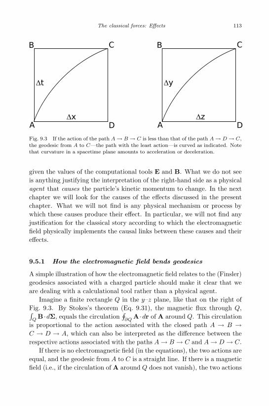
November 24, 2010 10:17 World Scientific Book - 9in x 6in main
The classical forces: Effects 113
Fig. 9.3 If the action of the path A → B → C is less than that of the path A → D → C,
the geodesic from A to C—the path with the least action—is curved as indicated. Notethat curvature in a spacetime plane amounts to acceleration or deceleration.
given the values of the computational tools E and B. What we do not see
is anything justifying the interpretation of the right-hand side as a physical
agent that causes the particle’s kinetic momentum to change. In the next
chapter we will look for the causes of the effects discussed in the present
chapter. What we will not find is any physical mechanism or process by
which these causes produce their effect. In particular, we will not find any
justification for the classical story according to which the electromagnetic
field physically implements the causal links between these causes and their
effects.
9.5.1 How the electromagnetic field bends geodesics
A simple illustration of how the electromagnetic field relates to the (Finsler)
geodesics associated with a charged particle should make it clear that we
are dealing with a calculational tool rather than a physical agent.
Imagine a finite rectangle Q in the y–z plane, like that on the right of
Fig. 9.3. By Stokes’s theorem (Eq. 9.31), the magnetic flux through Q,∫
QB ·dΣ, equals the circulation
∮
∂QA ·dr of A around Q. This circulation
is proportional to the action associated with the closed path A → B →C → D → A, which can also be interpreted as the difference between the
respective actions associated with the paths A→ B → C and A→ D → C.
If there is no electromagnetic field (in the equations), the two actions are
equal, and the geodesic from A to C is a straight line. If there is a magnetic
field (i.e., if the circulation of A around Q does not vanish), the two actions

November 24, 2010 10:17 World Scientific Book - 9in x 6in main
114 The World According to Quantum Mechanics
differ: one path is longer than the other (in terms of the geometry defined
by the potentials V and A). As a result, the geodesic from A to C is curved.
If A→ D → C is longer than A→ B → C, then the shortest path from A
to C is closer to A→ B → C than to A→ D → C.
Next, imagine an infinitesimal rectangle in the x–t plane, with corners
A = (−t/2,−dx/2, 0, 0), B = (dt/2,−dx/2, 0, 0), C = (dt/2, dx/2, 0, 0),
and D = (−dt/2, dx/2, 0, 0). Let us calculate the circulation around it of
the potential part −qV dt+(q/c)A ·dr of the action differential (9.18). The
contributions from the four sides are, respectively,
AB : −qV (0,−dx/2, 0, 0) dt = −q(
V (0, 0, 0, 0)− ∂V
∂x
dx
2
)
dt ,
BC : (q/c)Ax(dt/2, 0, 0, 0) dx = (q/c)
(
Ax(0, 0, 0, 0) +∂Ax
∂t
dt
2
)
dx ,
CD : qV (0, dx/2, 0, 0) dt = q
(
V (0, 0, 0, 0) +∂V
∂x
dx
2
)
dt ,
DA : −(q/c)Ax(−dt/2, 0, 0, 0) dx = −(q/c)
(
Ax(0, 0, 0, 0)− ∂Ax
∂t
dt
2
)
dx ,
and they add up to
q
(∂V
∂x+
1
c
∂Ax
∂t
)
dt dx = −qEx dt dx . (9.51)
If we now add the circulations associated with the infinitesimal rectangles
that make up a finite rectangle Q, like that on the left of Fig. 9.3, we
again find that contributions from adjacent sides cancel (cf. Sec. 9.4.1). As
a result, the circulation of the action around Q is given by the integral
−q∫
QEx(t, r) dt dx.
This circulation can again be interpreted as the difference between the
respective actions associated with the paths A→ B → C and A→ D → C.
If there is no electromagnetic field (in the equations), these actions are
equal, and the geodesic from A to C is a straight line. Because we are now
dealing with a spacetime plane containing the time axis, this means that
the particle travels with a constant speed. If there is an electric field (i.e.,
if the circulation of the action around Q does not vanish), the two actions
differ: one path is longer than the other (again, in terms of the geometry
defined by V and A). As a result, the geodesic from A to C is curved.
In a plane containing the time axis, this means that the particle’s speed
changes; the particle is accelerating or decelerating.

November 24, 2010 10:17 World Scientific Book - 9in x 6in main
The classical forces: Effects 115
9.6 Curved spacetime
So far in this chapter we have been concerned with the most straightforward
way of formulating effects on the motion of a (scalar) particle, regardless
of their causes. This consisted in adding to the action differential for a
free particle a term that is linear in both dt and dr, and it led to the
differential geometry defined by (9.18). The latter describes all so-called
electromagnetic effects on the motion of a (scalar) particle, both quantum-
mechanically, via propagators, and classically, in terms of the curvature of
geodesics.
There is one more way of incorporating effects on the motion of a (scalar)
particle. It is to unfix the spacetime geometry implicit in the action dif-
ferential for a free particle, dS = −mc2 ds. To implement this possibility,
we begin by recasting the scalar product (6.53) of two 4-vectors into the
following form:
(~a,~b) =
3∑
i=0
3∑
k=0
gik aibk. (9.52)
The vector components are labeled by superscript indices running from 0
to 3—for example, (at, ax, ay, az) = (a0, a1, a2, a3)—and the numbers gik
are as follows:
g00 g01 g02 g03g10 g11 g12 g13g20 g21 g22 g23g30 g31 g32 g33
=
1 0 0 0
0 −1 0 0
0 0 −1 0
0 0 0 −1
. (9.53)
When liberated from the specific values on the right-hand side, these num-
bers form the components of a pseudo-Riemannian metric—“Riemannian”
because this metric is at the heart of the differential geometry originally
formulated by Bernhard Riemann, and “pseudo” because even its “flat”
form (given by the right-hand side of Eq. 9.53) is non-Euclidean, owing to
the different signs of the diagonal terms. Because the scalar product (9.52)
of two 4-vectors is symmetric, (~a,~b) = (~b,~a), we can require that the metric
components be symmetric, too: gik = gki.
The metric is a machine with two input slots. If we insert into both
slots the infinitesimal 4-vector with components (dx0, dx1, dx2, dx3) =
(c dt, dx, dy, dz), we obtain (recalling Eq. 6.45) the 4-scalar
3∑
i=0
3∑
k=0
gik dxi dxk = c2 dt2 − dr · dr = c2 ds2 . (9.54)

November 24, 2010 10:17 World Scientific Book - 9in x 6in main
116 The World According to Quantum Mechanics
If we adopt the convention (due to Einstein) that equal spacetime indices
occurring twice (once as subscript and once as superscript) are summed
automatically, without having to write those bulky summation symbols,
we can substitute gik dxi dxk for c2 ds2, and we can cast the action differ-
ential for a particle subject to such effects as are represented by a pseudo-
Riemannian geometry, into the form
dS = −mc√
gik dxi dxk . (9.55)
9.6.1 Geodesic equations for curved spacetime
By allowing the metric components gik to differ from spacetime point to
spacetime point, we make room for another kind of influence on the motion
of a particle, regardless of what is exerting it. Its effects will again be
mathematically expressed as modifications of the actions associated with
spacetime paths, and classical particles will again follow the geodesics of
the corresponding differential geometry.
The geodesic equations for the geometry defined by (9.55) can be ob-
tained in much the same way we obtained the geodesic equations (9.13)
and (9.14) for the geometry defined by the action differential (9.18). [For
the details, the reader may consult Landau and Lifshitz (1975).] Here is
the result:
d2xi
ds2+ Γi
kl
dxk
ds
dxl
ds= 0 . (9.56)
The symbols
Γikl
Def=
1
2gim
(∂gmk
∂xl+∂gml
∂xk− ∂gkl
∂xm
)
(9.57)
are the so-called connection coefficients, also known as “Christoffel sym-
bols.” (Superscript indices in denominators are to be treated like subscript
indices in numerators.)
9.6.2 Raising and lowering indices
Before we can enter into the physical meaning of the geodesic equations
(9.56), we need to know how covariant components (having subscript in-
dices) are transformed into contravariant components (having superscript
indices), and vice versa. The covariant components of a 4-vector are defined
by
aiDef= gik a
k . (9.58)
November 24, 2010 10:17 World Scientific Book - 9in x 6in main
The classical forces: Effects 117
This tells us how to lower indices. Identical indices on different sides of an
equation can be raised or lowered simultaneously. Thus ai = gik a
k. This
tells us that
gik =
{0 if i 6= k
1 if i = k. (9.59)
(Because of the symmetry of the metric, gik can be read either as gi
k or as
gki.) The definition (9.58) allows us to cast Eq. (9.52) into the simple form
(~a,~b) = akbk. (9.60)
By the symmetry of the scalar product, akbk = akbk. This holds for any
matching pair of indices: the covariant index can be raised if the contravari-
ant index is lowered at the same time. Thus we also have that
ai = gik ak . (9.61)
This tells us how to raise indices.
9.6.3 Curvature
The curvature of a 2-dimensional surface (such as the surface of the sphere
in Fig. 9.4) is readily detected by us since we have the luxury of a conscious-
ness capable of visualizing 3-dimensional objects. But how do we detect the
curvature of a 3-dimensional hypersurface if we do not have the luxury of a
consciousness capable of visualizing 4-dimensional objects? Or how do we
detect the curvature of a 3-dimensional structure if this is not embedded in
a 4-dimensional space? And, harder still, how do we detect the curvature
of 4-dimensional spacetime?
Put yourself in the (2-dimensional) shoes of a flatlander.3 You live in
a 2-dimensional world and cannot leave it; you cannot imagine a third
dimension perpendicular to your own two. How can you find out whether
your world is curved?
Here is a possible test: draw a circle and measure its circumference C;
draw a diameter of the circle and measure its length D; take the ratio C/D.
If it differs from π, your world is curved. If it is smaller than π, you may
live on the surface of a sphere (Fig. 9.4). If it is larger than π, you may live
on a saddle-shaped surface.
3Flatland: A Romance of Many Dimensions is an 1884 satirical novella by the Englishschoolmaster Edwin A. Abbott. In a foreword to one of its many publications, Isaac Asi-mov wrote that it was “the best introduction one can find into the manner of perceivingdimensions.”
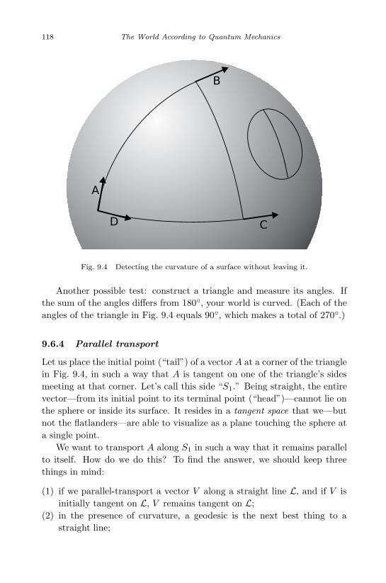
November 24, 2010 10:17 World Scientific Book - 9in x 6in main
118 The World According to Quantum Mechanics
Fig. 9.4 Detecting the curvature of a surface without leaving it.
Another possible test: construct a triangle and measure its angles. If
the sum of the angles differs from 180◦, your world is curved. (Each of the
angles of the triangle in Fig. 9.4 equals 90◦, which makes a total of 270◦.)
9.6.4 Parallel transport
Let us place the initial point (“tail”) of a vector A at a corner of the triangle
in Fig. 9.4, in such a way that A is tangent on one of the triangle’s sides
meeting at that corner. Let’s call this side “S1.” Being straight, the entire
vector—from its initial point to its terminal point (“head”)—cannot lie on
the sphere or inside its surface. It resides in a tangent space that we—but
not the flatlanders—are able to visualize as a plane touching the sphere at
a single point.
We want to transport A along S1 in such a way that it remains parallel
to itself. How do we do this? To find the answer, we should keep three
things in mind:
(1) if we parallel-transport a vector V along a straight line L, and if V is
initially tangent on L, V remains tangent on L;
(2) in the presence of curvature, a geodesic is the next best thing to a
straight line;

November 24, 2010 10:17 World Scientific Book - 9in x 6in main
The classical forces: Effects 119
(3) the sides of a triangle on the surface of a sphere are geodesics. (This is
part of what “triangle” means on the surface of a sphere.)
We shall accordingly make it part of what “parallel transport” means on
the surface of a sphere that geodesics parallel transport their tangent vec-
tors. For (2-dimensional) surfaces, a more general statement holds: if V
is parallel transported along a geodesic G, and if T is a co-moving tangent
vector on G originating at the tail of V , the angle between V and G remains
constant.
Thus when A (in Fig. 9.4) reaches the other end of S1, it is equal
to B; when subsequently parallel transported along the second side of the
triangle, it becomes equal to C, and if it is then parallel transported along
the third side, it becomes equal toD. This illustrates another manifestation
of curvature: if a vector is parallel transported along a closed curve, so that
it returns to its starting point and remains parallel to itself all along the
way, it will yet, in general, point in a different direction than it did at the
outset.
In 4-dimensional spacetime we can perform an analogous test. To find
out if spacetime is warped, we may transport gyroscopes, initially pointing
in the same direction, along different routes from a common starting point A
to a common end point B. In a curved spacetime, they generally won’t point
in the same direction when they meet again at B.
To find out more, let ~v be a vector field in spacetime. We wish to know
the difference D~v between ~v(P) and ~v(P ′) if the spacetime points P and
P ′ are separated by an infinitesimal vector with components dxk. Because
the two vectors are situated in different tangent spaces—flat spacetimes
“touching” curved spacetime at the respective points P and P ′—we need
to take into account that the basis vectors of these tangent spaces may
differ. If they are the same, the components of the two vectors simply
differ by
Dvi = dvi =∂vi
∂xldxl. (9.62)
If they are not the same, a compensatory term must be added. Because Pand P ′ are an infinitesimal distance apart, this term will be linear in the
components vi and dxk . Thus
Dvi = dvi + Γi
klvkdxl =
(∂vi
∂xl+ Γ
i
klvk
)
dxl. (9.63)
Now suppose that P and P ′ are the endpoints of an infinitesimal segment
dG of a geodesics G, and that ~u is a tangent vector on G located at P . Let us

November 24, 2010 10:17 World Scientific Book - 9in x 6in main
120 The World According to Quantum Mechanics
use a specific tangent vector, the 4-velocity ui = dxi/c ds. (Here we conform
to the convention of referring to a 4-vector ~v by a generic component vi.)
Problem 9.6. ui = dxi/c ds satisfies uiui = 1.
Because geodesics parallel transport their tangent vectors, there will be no
difference between ui(P) and ui(P ′):
Dui = dui + Γi
klukdxl = 0 . (9.64)
Divide by ds to find that
d2xi
ds2+ Γ
i
kl
dxk
ds
dxl
ds= 0 . (9.65)
Both Eq. (9.56) and Eq. (9.65) characterizes the geodesics of the geometry
defined by the action differential (9.55). The former defines them as the
curves that minimize (or maximize) their actions, whereas the latter defines
them as the curves that parallel transport their tangent vectors. Since the
two equations are therefore identical, Γi
kl is given by Eq. (9.57)
A useful abbreviation,
vi;l
Def=
∂vi
∂xl+ Γ i
klvk , (9.66)
allows us to write Dvi = vi;l dx
l for the covariant derivative (9.63).
9.7 Gravity
While the geodesics defined by Eqs. (9.14) and (9.18) describe the classi-
cal effects of what history has led us to call “the electromagnetic force,”
the geodesics defined by Eq. (9.56) describe the classical effects of what
history has led us to call “the gravitational force” or “gravity.” One
crucial difference between the corresponding geometries is that the for-
mer is particle-specific: it depends, through Eq. (9.18), on the masses
and the charges of the particles affected. Equation (9.56), by contrast,
is universal. It contains no particle-specific parameters, and for this
reason it is customary to attribute the latter geometry to spacetime
itself.
As we shall see in Part 3, quantum mechanics provides sufficient ground
for rejecting the notion of an intrinsically differentiated and intrinsically
structured spacetime. For the moment, however, I shall confine myself
to illustrating that the mathematical description of gravitational effects in

November 24, 2010 10:17 World Scientific Book - 9in x 6in main
The classical forces: Effects 121
Fig. 9.5 The spacetime curvatures of the trajectories of a ball and of a bullet near theEarth’s surface.
terms of a universal spacetime geometry is not as counterintuitive as it
might seem at first. To this end we will estimate the spacetime curvatures
of two trajectories observed near the Earth’s surface:
• A ball is thrown so that it rises to a height of about h1 = 5 m, covers
a distance of 10 m, and hits the ground after 2 seconds.
• A bullet is fired so that it rises to a height of about h2 = 5× 10⁻⁴ m,
covers the same distance, and hits the ground after 0.02 seconds.
In space the curvatures of these trajectories are obviously very different, but
not in spacetime. The distances traveled in spacetime are essentially the
times of travel multiplied by the speed of light, i.e., d1 = 2c = 6× 10⁸m for
the ball and d2 = 0.02 c = 6× 10⁶m for the bullet (Fig. 9.5). According to
Pythagoras, the radius of curvature r is related to the parameters h and d
via (r−h)2+(d/2)2 = r2. Because h� d < r, we ignore the term quadratic
in h and obtain r = d2/8h. This works out at r = 9× 10¹⁵ m ≈ 1 light year
for both the ball and the bullet.

November 24, 2010 10:17 World Scientific Book - 9in x 6in main
This page intentionally left blankThis page intentionally left blank

December 23, 2010 10:25 World Scientific Book - 9in x 6in main
Chapter 10
The classical forces: Causes
10.1 Gauge invariance
Problem 10.1. (∗) Adding (q/c) df(t, r) to the action differential dS in-
duces the following transformation of the propagator (9.1):
〈rB , tB|rA, tA〉 → e(i/~)(q/c) f(tB ,rB)〈rB , tB|rA, tA〉 e−(i/~)(q/c) f(tA,rA) .
(10.1)
It follows that Eq. (7.12),
ψ(rB, tB) =
∫
d3rA 〈rB , tB|rA, tA〉ψ(rA, tA) ,
is invariant under the transformation (10.1), provided that this is combined
with the phase transformation
ψ(t, r)→ e(i/~)(q/c) f(t,r)ψ(t, r) . (10.2)
Problem 10.2. (∗) Adding (q/c) df(t, r) to the action differential dS given
by Eq. (7.8) is equivalent to the following transformation of the potentials:
V → V − 1
c
∂f
∂t, A→ A+
∂f
∂r. (10.3)
In classical physics, one refers to (10.3) as a gauge transformation. In
quantum physics, one usually understands by this term the combination of
(10.3) with (10.2).
Problem 10.3. The electric and magnetic fields (Eq. 9.48) are invariant
under the transformation (10.3).
123

November 24, 2010 10:17 World Scientific Book - 9in x 6in main
124 The World According to Quantum Mechanics
10.2 Fuzzy potentials
The task now before us is to link to their causes the effects that we
have just learned to describe in mathematical language. What, then,
are their causes? Here we cannot proceed further without making spe-
cific assumptions. The causes could include minds, spirits, elves, gob-
lins—what have you. Goblins appear to have been at work at the LHC,
but otherwise we just don’t know. We shall simply assume that we
are dealing with particles and nothing but particles and that, therefore,
the behavior of particles (including their aggregates) is affected by noth-
ing but particles (including their aggregates). We shall however keep
an open mind as to the nature of the things we call “particles” and
“aggregates.”
So far we have assumed that the potentials V (t, r) and A(t, r) have exact
values. Yet particles are fuzzy : neither their positions nor their momenta
are in possession of exact values. If these potentials represent effects that
particles have on particles, their values cannot be sharp. Fuzzy causes have
fuzzy effects.
So how do we make room for fuzzy potentials? In much the same way
that we made room for fuzzy particles! In the case of a single particle, this
meant calculating the propagator 〈r2, t2|r1, t1〉 by summing over spacetime
paths leading from (r1, t1) to (r2, t2). For a system with N degrees of
freedom, this meant calculating the propagator 〈P2, t2|P1, t1〉 by summing
over paths from a point (P1, t1) to a point (P2, t2) in the system’s N+1-
dimensional configuration spacetime (Eq. 9.3). Presently we are dealing
with a mathematical device that allows us to calculate effects of a partic-
ular type. This device—the 4-potential ~A = (V,A)—has a denumerably
infinite number of degrees of freedom and a configuration space with as
many dimensions. The configuration A obtaining at the time t specifies
the components of ~A associated with each point r in the 3-dimensional
hyperplane associated with t.1
To make room for fuzzy potentials, we thus calculate the propagator
〈A2, t2|A1, t1〉 by summing over all paths leading from a given configuration
1Like the real line or the complex plane, this hypersurface forms a non-denumerableset. How can the configuration of A be specified by a denumerable set of values? Theanswer is that we take ~A to be well-behaved in the sense spelled out in Sec. 3.3. Just asa well-behaved function of a single variable x can be fully specified by a countable setof parameters—for instance, the coefficients of its Taylor series—so can a well-behaved4-vector field.

November 24, 2010 10:17 World Scientific Book - 9in x 6in main
The classical forces: Causes 125
A1 (obtaining at the time t1) to a given configuration A2 (obtaining at t2):
〈A2, t2|A1, t1〉 =∫
DC e(i/~) SA[C]. (10.4)
10.2.1 Lagrange function and Lagrange density
To find the appropriate action SA[C], we begin by observing that the action
differential dS(t, r, dt, dr) associated with an infinitesimal segment of a
spacetime path can be cast into the form
dS = L(t, r,v) dt . (10.5)
To see this, we only have to substitute 1/dt for the parameter u in Eq. (7.7).
The immediate result is
dS(t, r,v) =dS(t, r, dt, dr)
dt.
But now the notation is no longer appropriate, for the left-hand side, having
ceased to depend on infinitesimal quantities, has itself ceased to be an
infinitesimal quantity. In its place we write L(t, r,v). L is known as a
Lagrange function.
Problem 10.4. (∗) Write down the Lagrange function for the action dif-
ferential (7.8).
The homogeneity of dS expressed by Eq. (7.7) allowed us to interpret dS as
defining a differential geometry. If we interpret dSA as defining a differential
geometry in the configuration spacetime of the potentials, then we also have
that
dSA = LA(A, dA/dt) dt . (10.6)
Consistency with special relativity, however, requires that the four dimen-
sions of spacetime be treated on an equal footing (apart from the sign
difference in Eq. 6.45). This means that SA must be expressible as an
integral over spacetime, rather than as an integral over time only:
SA =1
c
∫
LA(Ak, ∂Ak/∂xi) d4x . (10.7)
The Lagrange density LA (also known simply as the Lagrangian) is a
4-scalar, and d4x stands for the 4-volume element (c dt) dx dy dz.
In classical physics, the potentials serve to connect physical effects with
their physical causes, but only as calculational tools. Given the causes, we
calculate the potentials, and given the potentials, we calculate the effects.

November 24, 2010 10:17 World Scientific Book - 9in x 6in main
126 The World According to Quantum Mechanics
Since the effects are represented by gauge-invariant combinations of the
potentials (E and B), it makes sense to require that the causes determine
only these combinations. We therefore require that LA, too, be invariant
under the transformation (10.2).2 If we further require that the effects
that charges have on charges are additive, in the sense that the combined
effect of two charges A and B on a third charge is the (vectorial) sum of
the individual effects produced by A and B, then we are left with a single
candidate, the Lagrangian
LA =1
8π(E2 −B2) . (10.8)
10.3 Maxwell’s equations
As the fundamental equation of classical electrodynamics are formulated in
terms of a current rather than in terms of particles, we replace the charge q
in Eq. (9.18) by a charge density ρ and integrate over space as well:
SAM = −∫
(qV − q
cA · dv) dt −→ − 1
c2
∫
(cρV −A · j) d4x . (10.9)
The current density j = ρv denotes the flow of charge per unit area per
unit time.
We have omitted SM = −mc2ds, the term in Eq. (9.18) that does not
contain the potentials. When we established how the classical trajectories
of charged particles depend on the potentials, we took the values of the
potentials as given. We therefore had no need to include SA. Presently
we wish to determine how E and B depend on the distribution and mo-
tion of particles (represented, respectively, by ρ and j). Since the distri-
bution and motion of particles is now taken as given, we do not need to
include SM.
To streamline our task, we define the tensor components
Fik =∂Ak
∂xi− ∂Ai
∂xk, (10.10)
the components Ak of ~A being given by (V,Ax, Ay, Az). (Tensor compo-
nents like Fik transform like a product of vector components CiDk.)
2There is a deeper reason for this requirement: it makes quantum electrodynamicsrenormalizable (Sec. 15.8).

November 24, 2010 10:17 World Scientific Book - 9in x 6in main
The classical forces: Causes 127
Problem 10.5.
F00 F01 F02 F03
F10 F11 F12 F13
F20 F21 F22 F23
F30 F31 F32 F33
=
0 Ex Ey Ez
−Ex 0 −Bz By
−Ey Bz 0 −Bx
−Ez −By Bx 0
. (10.11)
If in addition we introduce the 4-current ~J with components Jk =
(cρ, jx, jy, jz), we can write the relevant action more compactly as
SAM + SA = − 1
c2
∫ (
AkJk +
c
16πFikF
ik)
d4x . (10.12)
Problem 10.6. This is the same as
− 1
c2
∫
(cρV −A · j) d4x+1
8πc
∫
(E2 −B2) d4x . (10.13)
If δ(SAM + SA) is to vanish under any infinitesimal variation δAk of the
potentials, we must have that∫ [
(δAk) Jk +c
8π(δFik)F ik
]
d4x = 0 . (10.14)
Here we have made use of δ(FikFik) = 2(δFik)F ik, which holds for much
the same reason as dx2 = 2x dx. Because the antisymmetry of Fik (i.e.,
Fik = −Fki) allows us to write
F ik(δFik) = 2F ik ∂ δAk
∂xi, (10.15)
Eq. (10.14) becomes∫ [
(δAk) Jk +c
4πF ik ∂ δAk
∂xi
]
d4x = 0 . (10.16)
Integrating by parts, we obtain∫
F ik ∂ δAk
∂xid4x =
∫∂
∂xi
(
F ik δAk
)
d4x−∫∂F ik
∂xiδAk d
4x . (10.17)
The 4-dimensional version of Gauss’s law (9.37) allows us to convert the
first integral on the right-hand side into an integral over a spatiotemporal
boundary. At the spatial “boundary” (infinity) the potentials—at any rate,
their gauge-invariant combinations—are assumed to vanish, and at the tem-
poral boundaries the configurations A1 and A2 are fixed (δA1 = δA2 = 0).
This integral therefore equals zero, so Eq. (10.14) takes the form∫ (
Jk − c
4π
∂F ik
∂xi
)
δAk d4x = 0 . (10.18)
November 24, 2010 10:17 World Scientific Book - 9in x 6in main
128 The World According to Quantum Mechanics
Thus if SAM + SA is to be stationary for every (infinitesimal) variation
δAk, the potentials must satisfy the condition
∂F ik
∂xi=
4π
cJk. (10.19)
Problem 10.7. Equation (10.19) is equivalent to
∂
∂r· E = 4πρ ,
∂
∂r×B =
1
c
∂E
∂t+
4π
cj . (10.20)
This is the second pair of Maxwell’s equations. The first pair,
∂
∂r·B = 0 ,
∂
∂r×E = −1
c
∂B
∂t, (10.21)
follows from the definitions (9.48) of E and B and the identities (9.33) and
(9.40). Together with the Lorentz force law (9.50), these four equations
make up the set of fundamental equations of the classical electromagnetic
theory.
The following problem illustrates that electricity and magnetism are two
sides of the same coin: what counts as a magnetic effect if one reference
frame is used, may count as an electric effect if a different frame is used,
and vice versa.
Problem 10.8. (∗) Consider a long current-bearing wire. Situated near the
wire is a charged particle. Described in terms of one inertial frame (F1),
the particle is at rest. Described in terms of another inertial frame (F2),
the particle moves parallel to the wire with a constant speed. In F2, the
particle experiences a force according to the magnetic term of the Lorentz
force law. In F1, this term vanishes, so the force acting on the particle must
be due to the electric term. What is the source of E in this frame?
10.3.1 Charge conservation
Problem 10.9. (∗) Use Eq. (10.19) to show that
∂Jk
∂xk= 0 . (10.22)
In 3-vector notation this reads:
∂ρ
∂t= − ∂
∂r· j . (10.23)

November 24, 2010 10:17 World Scientific Book - 9in x 6in main
The classical forces: Causes 129
Integrating both sides over a spatial region R with an unmoving boundary
∂R, we obtain
∂Q(R)
∂t=
∂
∂t
∫
R
ρ d3r = −∫
R
∂
∂r· j d3r = −
∫
∂R
j · dΣ . (10.24)
On the far right we made use of Gauss’s law (9.37). Equation (10.24) tells
us that the rate at which the charge Q(R) inside R increases equals minus
the rate at which charge flows outward across the boundary ∂R of R. It is,
in other words, a statement of the conservation of charge. Equation (10.23)
is known as an equation of continuity.
10.4 A fuzzy metric
Our next task is to link the effects of gravity to their causes. Once again
we assume that we are dealing with particles and nothing but particles
and that, therefore, the behavior of particles (including their aggregates) is
affected by nothing but particles (including their aggregates).
So far the components gik of the metric have been taken to be in posses-
sion of exact values. Yet, again, particles are fuzzy : neither their positions
nor their momenta are in possession of exact values. If the metric represents
effects that particles have on particles, its components cannot be sharp.
But now we run into a problem. As long as the metric is sharp, its
components can be treated as functions of spacetime points, at least in our
mathematical imagination. If the metric becomes fuzzy, so do the distances
between spacetime points. But it is distances that are physically accessible,
not spacetime points per se. Physically meaningful locations are defined
by the distances between them. If spacetime distances become fuzzy, it
becomes inconsistent to define the metric over a set of points that is locally
isomorphic with a set of quadruplets of real numbers—points that can be
labeled by spacetime coordinates. Physicists have not yet learned how to
successfully circumnavigate this conundrum. Perhaps this is the reason—or
at least one of the reasons—why we do not have a renormalizable quantum
theory of gravity yet.
Since the present theory’s lack of renormalizability does not prevent us
from expressing the fuzziness of the metric in terms of path integrals, we
can again use the principle of least action to obtain the classical theory.
Assuming that the particles and the potentials follow fixed paths in their
respective configuration spacetimes, we look for the conditions in which the
action is stationary under arbitrary infinitesimal variations of the metric.

November 24, 2010 10:17 World Scientific Book - 9in x 6in main
130 The World According to Quantum Mechanics
To be able to do so, we need a gravity term analogous to the term (10.7):
SG =1
c
∫
L(gik, ∂gik/∂xl)√−g d4x . (10.25)
In the presence of the metric, the volume element is given by√−g d4x. g is
the determinant of the metric, which is given by
g = εijkl g0i g1j g2k g3l , (10.26)
where
εijkl =
+1 if ijkl is an even permutation of 0123
−1 if ijkl is an odd permutation of 0123
0 if ijkl is not a permutation of 0123
(10.27)
As it turns out, there is no 4-scalar that can be constructed from the compo-
nents of the metric and their first derivatives. But there is just one 4-scalar
that additionally depends on the components’ second derivatives. This is
equal to the sum of two terms, one that depends on the components gik and
their first derivatives only, and one that can be converted into an irrelevant
boundary integral—irrelevant for reasons analogous to those given in the
paragraph following Eq. (10.17). This is the curvature scalar
R Def= gjlRjl = Rl
l , (10.28)
which is a contraction of the Ricci tensor
RjlDef= gikRijkl = Rk
jkl , (10.29)
which in turn is a contraction of the Riemann (curvature) tensor
Rijkl
Def=
∂Γijl
dxk−∂Γi
jk
dxl+ Γi
mkΓmjl − Γi
mlΓmjk . (10.30)
In Gaussian units, the wanted gravity term is therefore
SG =c3
16πG
∫
R√−g d4x , (10.31)
where G = 6.674× 10⁻¹¹ m3 kg−1s−2 is Newton’s gravitational constant.
10.4.1 Meaning of the curvature tensor
Imagine a quadrilateral whose sides are the infinitesimal vectors dui and
dvj . Take a vector Ak and parallel transport it about this quadrilateral—
first along dui, then along dvj , then along −duk, and finally along −dvl.
The resultant change in Ai is given by
δAi = −Riklm Ak dul dvm. (10.32)

December 23, 2010 10:25 World Scientific Book - 9in x 6in main
The classical forces: Causes 131
In other words, Riklm is a machine with three inputs and one output.
Insert the two sides of the quadrilateral into the last two input slots; insert
a vector that is transported about the quadrilateral into the first input slot;
get (minus) the resultant change of this vector.
10.4.2 Cosmological constant
In the weak-curvature limit, the action (10.31) yields Newton’s law of grav-
ity. It we do not regard this as necessary, the above constraints on the form
of the gravity term allow for the addition of a constant to the curvature
scalar R. The resulting action is usually written in this form:
SG =c3
16πG
∫
(R− 2Λ)√−g d4x . (10.33)
Λ is the so-called cosmological constant. According to recent astronomical
observations, it is small but not zero. Einstein originally introduced it to
allow for the possibility of a static universe. After the discovery, by Ed-
win Hubble, that the universe was in fact expanding, Einstein dismissed it
as “the greatest blunder” of his life. Today the cosmological constant is
seen as the most likely reason why the expansion of the universe is accel-
erating rather than slowing down, as one would expect from the mutual
gravitational attraction of the known forms of matter.
10.5 Einstein’s equation
The total action is now given by the sum SG + SM, where
SM =1
c
∫
LM√−g d4x . (10.34)
LM is a function of the matter variables and their first derivatives. (“Mat-
ter” now stands for everything but the metric.) The classical equations that
state the metric’s dependence on the distribution and motion of matter are
obtained by varying the metric while the matter variables are held fixed.
The result is the Einstein equation,
Rik −1
2Rgik + Λgik =
8πG
c4Tik , (10.35)
which is to Einstein’s theory of gravity—the general theory of relativity—
what Maxwell’s equations are to classical electrodynamics. The tensor Tikdepends on the specific form of LM.

November 24, 2010 10:17 World Scientific Book - 9in x 6in main
132 The World According to Quantum Mechanics
10.5.1 The energy–momentum tensor
In much the same way as Eq. (10.19) implies the conservation law (10.22)
(Problem 10.9), Eq. (10.35) implies the conservation law
T ik;k = 0 . (10.36)
The latter, however, only holds locally. If we chose a spacetime point
and a sufficiently small neighborhood containing it, we can (within this
neighborhood) use inertial coordinates, so that (within this neighborhood)
Eq. (10.36) takes the form of an equation of continuity—or, rather, four of
them, one for each index i:
∂T ik
∂xk= 0 . (10.37)
The conservation of the right-hand side of Eq. (10.19) and the conservation
of the right-hand side of Eq. (10.35) both are implied by the respective
left-hand sides of these equation. There is however another reason why the
tensor Tik on the right-hand side of Eq. (10.35) is (locally) conserved: the
matter action (10.34) can be shown to be invariant under transformations
of the metric that are locally equivalent to spacetime translations. This
justifies the identification of Tik in Eq. (10.35) with the energy–momentum
tensor of matter.
10.6 Aharonov–Bohm effect
Let us return to the two-slit experiment we discussed in Secs. 5.2–5.3. The
interference term contained the factor cos(k∆) (Eq. 5.3), where ∆ stood
for DR−DL, the difference between the distances of the detector from the
slits. Because the electron source is equidistant from the slits, ∆ is also the
difference between the lengths of the paths G→ L→ D and G→ R→ D.
We will call these paths L and R, respectively.
If the electron is subject to effects of the type that is represented by the
vector potential A, then (by Eq. 7.8) the phase associated with L contains
the additional term
q
c~
∫
LA · dr , (10.38)
and the phase associated with R contains the additional term
q
c~
∫
RA · dr . (10.39)

November 24, 2010 10:17 World Scientific Book - 9in x 6in main
The classical forces: Causes 133
Fig. 10.1 The vector potential and the magnetic field associated with a current bearing
solenoid.
The difference between these terms is an integral over the loop G → L →D → R→ G,
q
c~
∫
LA · dr− q
c~
∫
RA · dr =
q
c~
∮
A · dr Def= φ . (10.40)
If a vector potential is present (in the equations), the interference term thus
contains the factor cos(k∆ + φ). Invoking Stokes’s theorem (Eq. 9.31) and
the definition of the magnetic field (Eq. 9.48), we find that the integral of
A along that loop equals the flux of B through any surface Σ bounded by
it:∮
A · dr =
∫
Σ
B · dΣ . (10.41)
What happens if a long, thin solenoid passes through the loop G → L →D → R → G, at a right angle to the plane containing the loop, such that
there is a clear distance between it and the loop? If a current is flowing in
the solenoid, then there is—on paper— a magnetic field (Fig. 10.1), and if
there is no electric field (or only a static one), then, according to Maxwell’s
equations (10.20), the curl of this magnetic field is related to the density of
the current via
∂
∂r×B =
4π
cj . (10.42)

November 24, 2010 10:17 World Scientific Book - 9in x 6in main
134 The World According to Quantum Mechanics
The magnetic field outside the solenoid can be made arbitrarily weak by
making the solenoid sufficiently long. Essentially, therefore,
φ =q
c~
∫
Σ
B · dΣ . (10.43)
Because φ depends on the current flowing in the solenoid, the interference
pattern observed under the conditions stipulated by Rule B can be shifted
to the left or to the right by altering the strength and/or the direction of
the current.
This effect could easily have been predicted in the late 1920’s, by which
time all the necessary physics was in place. Yet by many accounts it was
predicted only three decades later, by Aharonov and Bohm (1959).3
10.7 Fact and fiction in the world of classical physics
Why did it take that long to predict such a remarkable effect? It is no excuse
that classical electrodynamics can be formulated exclusively in terms of E
and B, nor that the four components of V and A, which uniquely determine
the six components of E and B, are themselves not unique (Sec. 10.1). For
it was well known that the Schrodinger equation could accommodate elec-
tromagnetic effects only in terms of the potentials V and A (see Eq. 7.23),
and that loop integrals of A were gauge-invariant. Why was it neverthe-
less a widely held view that the potentials “have no physical meaning and
are introduced solely for the purpose of mathematical simplification of the
equations” [Rohrlich (1965)]?
What is implied by Rohrlich’s remark is that E and B have a kind of
physical meaning that the potentials lack. The general idea at the time
was that the electromagnetic field is a physical entity in its own right; it is
locally acted upon by charges, it locally acts on charges, and it mediates the
action of charges on charges by locally acting on itself. At the heart of this
notion is the so-called “principle of local action,” felicitously articulated by
DeWitt and Graham (1971) in an American Journal of Physics resource
letter:
Physicists are, at bottom, a naive breed, forever trying to come to termswith the “world out there” by methods which, however imaginative andrefined, involve in essence the same element of contact as a well-placedkick.
3Actually it was first predicted two decades later [Ehrenberg and Siday (1949)], but itmade a splash only after the publication of the paper by Aharonov and Bohm. This wasfollowed by an actual demonstration of the effect in less than a year.

November 24, 2010 10:17 World Scientific Book - 9in x 6in main
The classical forces: Causes 135
With the notable exception of Roger Boscovich, a Croatian physicist and
philosopher who flourished in the 18th Century, it does not seem to have
occurred to anyone that local action is as unintelligible as the apparent
ability of material objects to act where they are not, which the principle of
local action has purportedly explained away.4
If it is believed that electromagnetic effects on charges are locally pro-
duced by E and B, rather than at a distance by the distribution and motion
of charges, then something like the Aharonov–Bohm effect cannot be fore-
seen, for neither E nor B is significantly different from zero along the two
alternative electron paths. The lesson we have learned (or ought to have
learned) from the history of this effect is that neither the potentials nor
the fields should be thought of as physical entities in their own right. They
both are computational tools.
What about gravitational effects? Here, too, the objects acted upon
follow the geodesics of a differential geometry, and the consequences of
being acted upon are represented by the curvature of this geometry. In
the electromagnetic case, the curvature depends not only on the objects
that act but also on the objects that are acted upon, through their masses
and charges. In the gravitational case, the curvature is independent of
the objects acted upon. Does this warrant the reification of the geometry
representing gravitational effects? Or is it simply an instance of what math-
ematician and philosopher A.N. Whitehead (1997) has called “the fallacy
of misplaced concreteness”?
Remember how we got to this point. We were looking for propagators for
particles acted upon by particles. We found two mathematical constructs
that could be used to incorporate into the propagators of particles the effects
that particles have on particles—the 4-potential (V,A) and the metric. To
take into account the fuzziness of the particles acted upon, we summed over
paths in their configuration spacetime. To take into account the fuzziness of
the potentials and the metric, we summed over paths in their configuration
spacetimes. We then obtained the laws of classical physics by taking the
classical limit—the limit in which the fuzziness that “fluffs out” matter
disappears and a single extremal path survives (for the particles as well as
for the potentials and the metric). In this limit, the quantum-mechanical
4The impression that local action is intelligible derives from the familiarity of experi-ences like pulling a rope or pushing a stalled car. Why do the pushing hands not passright through the car? Taking a microscopic look at what happens between the surfaceof the car and the surfaces of the pushing hands, we discover that this apparently localaction involves net interatomic and intermolecular repulsive forces that act at a distance.

December 23, 2010 10:25 World Scientific Book - 9in x 6in main
136 The World According to Quantum Mechanics
probability algorithms degenerate into trivial probability algorithms, which
only assigns trivial probabilities (either 0 or 1).
A trivial probability algorithm—represented by a point in some phase
space—can be interpreted as a state in the classical sense of the word: a
collection of possessed properties (Sec. 8.1). What happens in the classical
limit, then, is that the quantum laws, which correlate the probabilities of
measurement outcomes probabilistically, degenerate into laws that correlate
intrinsically possessed properties or values deterministically. And because
deterministic correlations between intrinsically possessed properties or val-
ues lend themselves to causal interpretations, what happens is that the
quantum-mechanical algorithms, which serve to compute probabilities of
possible measurement outcomes on the basis of actual outcomes, degener-
ate into algorithms that serve to compute effects that matter has on matter.
What they do not is degenerate into descriptions of physical mechanisms
or processes by which matter acts on matter. As N. David Mermin (2009)
reminisced near the end of a distinguished career:
When I was an undergraduate learning classical electromagnetism, I wasenchanted by the revelation that electromagnetic fields were real. Farfrom being a clever calculational device for how some charged particlespush around other charged particles, they were just as real as the parti-cles themselves, most dramatically in the form of electromagnetic waves,which have energy and momentum of their own and can propagate longafter the source that gave rise to them has vanished.
That lovely vision of the reality of the classical electromagnetic fieldended when I learned as a graduate student that what Maxwell’s equa-tions actually describe are fields of operators on Hilbert space. Thoseoperators are quantum fields, which most people agree are not real butmerely spectacularly successful calculational devices. So real classicalelectromagnetic fields are nothing more (or less) than a simplification ina particular asymptotic regime (the classical limit) of a clever calcula-tional device. In other words, classical electromagnetic fields are anotherclever calculational device.
10.7.1 Retardation of effects and the invariant speed
In Newton’s theory, gravitational effects are instantaneous: the Earth is
attracted towards the Sun’s present position. It has been argued that this
was the reason why Newton could not but refuse to “frame hypotheses”
(about the mechanism by which gravity acts). Electromagnetic effects,
on the other hand, are retarded. The earliest time at which a solar flare
can affect us is about eight minutes later—the distance between the Sun

November 24, 2010 10:17 World Scientific Book - 9in x 6in main
The classical forces: Causes 137
and the Earth divided by the speed of light. According to a widely held
belief, the retardation of electromagnetic effects is what made it possible
to understand the mechanism by which these effects are transmitted.
Looking at it in another way, we reach the opposite conclusion. In
Secs. 6.4–6.5 we established the necessity of an invariant speed. (Reminder:
anything that “travels” with this speed in one inertial frame, will do so
in every other inertial frame.) In Newton’s theory the invariant speed is
infinite; in a relativistic theory it is finite. But regardless, what matters is
the existence of an invariant speed, inasmuch as it implies the existence of a
special kind of spatiotemporal relation between events: simultaneity, which
is absolute in Newton’s case, or the lightlike relation, which is absolute in
the relativistic case.
Suppose that an event e1 at (r1, t1) is the cause of an event e2 at (r2, t2).
The fact that e2 happens at t2, rather than at any other time, has two pos-
sible explanations, depending on whether the causal connection between
the events is mediated or unmediated. In the mediated case, t2 is deter-
mined by the speed of mediation. This could be the speed of a material
object traveling from r1 to r2, or the speed of a signal propagating in an
elastic medium, or something more exotic. In the unmediated case, t2 can
only be determined by the special spatiotemporal relation that is implied
by the existence of an invariant speed. In Newton’s theory, t2 is equal to t1,
while in a relativistic theory, t2 is given by t1 + |r2−r1|/c. A delay of e2 by
t2−t1 = |r2−r1|/c thus ought to be seen as the signature of an unmediated
causal connection between e1 and e2, rather than as an indication that the
causal relation between e1 and e2 is mediated by some physical process.
Again, in a non-relativistic theory, in which the stratification of space-
time into hypersurfaces of constant time (“simultaneities”) is absolute, en-
ergy and momentum are globally conserved: the total energy is the same in
all simultaneities, as is the total momentum. In a relativistic theory, where
the stratification of spacetime into simultaneities is frame-dependent, the
law of conservation of energy–momentum holds for every stratification. En-
ergy and momentum must therefore, in some sense, be locally conserved.5
5In a relativistic theory, energy–momentum cannot disappear in one place and instantlyre-appear in a different place, inasmuch as this would only hold with respect to one frameor class of frames. Described using a different frame, it would re-appear not only in adifferent place but also at a different time, so that energy-momentum would not even beglobally conserved.

November 24, 2010 10:17 World Scientific Book - 9in x 6in main
138 The World According to Quantum Mechanics
But in what sense? Like every local conservation law, the conserva-
tion of energy–momentum is a feature of the mathematical tools we em-
ploy to calculate the correlations between measurement outcomes—both
the probabilistic correlations of quantum physics and the deterministic cor-
relations of classical physics. For instance, it ensures that in all particle
“collision” experiments, and regardless of the reference frame used, the
total energy–momentum of the incoming particles equals the total energy–
momentum of the outgoing particles. (If some energy–momentum escapes
undetected, then the following conditional is warranted: if the escaped
energy–momentum were detected, it would agree with the local conserva-
tion law.)
But why give a thought to the meaning of the approximate laws of
classical physics, considering that “philosophically we are completely wrong
with the approximate law,” as Richard Feynman stressed at the beginning
of his famous Caltech lectures [Feynman et al. (1963), original emphasis]?
While learning the classical laws, most students of physics absorb a con-
siderable amount of metaphysical embroidery that does not bear scrutiny
in light of the underlying quantum laws. If this embroidery is not seen for
what it is and discarded in time, it needlessly frustrates students’ efforts
to make sense of quantum physics. Mermin (2009) was able to rid himself
of “our habit of inappropriately reifying our successful abstractions,” but
how many of us are?

December 23, 2010 10:25 World Scientific Book - 9in x 6in main
Chapter 11
Quantum mechanics resumed
11.1 The experiment of Elitzur and Vaidman
In the following experiment [Elitzur and Vaidman (1993)] a Mach–Zehnder
interferometer will be used. This consists of two beam splitters (BS1and BS2), two mirrors (M1 and M2), and two photodetectors (D1 and D2)
arranged as in Fig. 11.1. A particular twist of this experiment is the possi-
ble presence of a “bomb”—a photodetector that will explode if it absorbs
a photon. For simplicity’s sake we make the usual assumption that all
detectors (including the bomb) are 100% efficient.
Imagine, to begin with, that neither BS2 nor the bomb is present. A
photon beam enters BS1 from the left. Classically described, two beams
emerge, each with half the intensity of the incoming beam. Described in
quantum-mechanical terms, each photon has a 50% chance of being detected
by D1 (indicating that the photon was reflected upward by BS1) and an
equal chance of being detected by D2 (indicating that the photon went
horizontally through BS1).
If BS2 (but as yet no bomb) is present, Rule B applies. Here is what we
need to know about the amplitudes associated with the alternatives (reflec-
tion by M1 or reflection by M2): they are equal except that each reflection
causes a phase shift of π/2. (The magnitude of the phase shift depends on
the materials used. For the sake of convenience, we use materials for which
it equals π/2.) Such a phase shift is equivalent to the inclusion of a factor i.
Each of the alternatives leading to D1 involves two reflections, so the
corresponding amplitudes are equal (i2A, say). The probability of detection
by D1 thus is pB1 = |−A−A|2 = 4|A|2. The alternative leading to D2 via M1
involves three reflections, so that the corresponding amplitude has an extra
factor i3 = −i. The alternative leading to D2 via M2 involves a single
139

November 24, 2010 10:17 World Scientific Book - 9in x 6in main
140 The World According to Quantum Mechanics
Fig. 11.1 “Bomb testing” experiment of Elitzur and Vaidman.
reflection, and the corresponding amplitude has an extra factor +i. Because
the two amplitudes differ by a factor −1, the probability of detection by
D2, pB2 , equals 0. (Under the conditions stipulated by Rule A, we would
have that pA1 = pA
2 = 2|A|2.)Finally, if both BS2 and the bomb are present, the alternative taken by
the photon is measured. If the bomb explodes, we can conclude that the
photon went via M1, and if it does not explode, we can conclude that the
photon went via M2. If it went via M2, either photodetector responds with
probability 1/2. Thus:
• If the bomb is absent, D1 clicks every time (100%), and D2 never clicks
(0%).
• If the bomb is present, it explodes half of the time (50%), and if it
doesn’t explode, D1 and D2 are equally likely to respond (25% each).
Problem 11.1. Suppose that the bomb is present. Is it possible, with the
help of the present setup, to ascertain the presence of the bomb without
setting it off? Ponder this before you proceed.
The answer is affirmative, albeit only in 25% of the tests. If the bomb
explodes, which happens in 50% of the tests, we have failed. If the bomb

December 23, 2010 10:25 World Scientific Book - 9in x 6in main
Quantum mechanics resumed 141
is present and D1 responds, which happens in 25% of the tests, we have
learned nothing, for D1 also responds if the bomb is absent. But if D2
responds, which happens in 25% of the tests, we have succeeded, for D2
never responds if the bomb is absent.
When a version of this experiment was demonstrated at a science fair in
Groningen, the Netherlands, in 1995 [du Marchie van Voorthuysen (1996)],
the reactions of non-physicists differed markedly from those of physicists.
Everyone was perplexed, for the detection of the photon by D2 seems to
have contradictory implications:
• The bomb was present.
• The photon never came near the bomb.
If the photon never came near the bomb, how was it possible to learn
that the bomb was present? While most ordinary folks thought that some
physicist will eventually solve this puzzle, the physicists themselves were
decidedly less hopeful that a satisfactory explanation will be found.
11.2 Observables
Many students of quantum mechanics are more or less apodictically in-
formed that observables are self-adjoint operators, and that the possible
values of an observable are its eigenvalues. These statements would be
virtually self-evident if they were accompanied by sufficient emphasis on
the probabilistic nature of the mathematical tools of quantum mechanics,
which is rarely the case.
Consider a measurement whose possible outcomes are represented by
projectors |vk〉〈vk|, k = 1, 2, . . . . If the density operator is W, the corre-
sponding probabilities are 〈vk|W|vk〉, and their mean value is
〈v〉 =∑
k
vk〈vk|W|vk〉 . (11.1)
If the density operator is pure, W = |w〉〈w|, the probabilities are
〈vk|w〉 〈w|vk〉 = 〈w|vk〉 〈vk|w〉, and their mean value is
〈v〉 = 〈w|V|w〉 with V =∑
k
|vk〉vk〈vk| . (11.2)
Remembering the spectral theorem (8.30), we conclude that V is self-
adjoint, that the vectors |vk〉 are its eigenvectors, and that the values vkare the corresponding eigenvalues.

November 24, 2010 10:17 World Scientific Book - 9in x 6in main
142 The World According to Quantum Mechanics
11.3 The continuous case
When dealing with continuous observables,1 it is often more convenient to
work with the position representation ψ(x) = 〈x|ψ〉 of a Dirac vector |ψ〉than to work with the Dirac vector itself. For example, we may write the
mean value (4.14) either as
〈x〉 = 〈ψ|X|ψ〉 with X =
∫
|x〉x 〈x| dxor as
〈x〉 =
∫
ψ∗(x) x ψ(x) dx =
∫
〈ψ|x〉 x 〈x|ψ〉 dx with x = x .
Using the position representation has the advantage that applying x to ψ(x)
boils down to multiplying ψ(x) by x.
Another representation convenient to work with is the momentum
representation ψ(k) = 〈k|ψ〉 of a Dirac vector |ψ〉. It allows us to cast
the mean value (4.16) into the form
〈p〉 =
∫
〈ψ|k〉 p 〈k|ψ〉 dk (11.3)
with p = ~k. The momentum operator in the position representation has
to satisfy
〈p〉 =
∫
〈ψ|x〉 p 〈x|ψ〉 dx .
We will now demonstrate with the help of Eq. (4.9) that p = (~/i)(∂/∂x)
fits the bill.
〈p〉 =
∫
ψ∗(x)~
i
∂
∂xψ(x) dx
=1
2π
∫ [∫
ψ∗(k′, t) e−ik′xdk′
]~
i
∂
∂x
[∫
ψ(k, t) eikxdk
]
dx
=1
2π
∫ [∫
ψ∗(k′, t) e−ik′xdk′
] [∫
ψ(k, t) ~k eikxdk
]
dx
=
∫ ∫
ψ∗(k′, t) ~k ψ(k, t)
[1
2π
∫
ei(k−k′)xdx
]
dk′ dk .
Because the square bracket in the last line is a way of writing the delta
distribution δ(k − k′) (Sec. 8.12.2), we end up with
〈p〉 =
∫ ∫
ψ∗(k′, t) ~k ψ(k, t) δ(k − k′) dk′ dk =
∫
ψ∗(k, t) ~k ψ(k, t) dk .
This is Eq. (11.3) with p = ~k.1It would be more correct to speak of observables whose possible measurement outcomes
form a denumerable set of mutually disjoint subsets of a non-denumerable set.

November 24, 2010 10:17 World Scientific Book - 9in x 6in main
Quantum mechanics resumed 143
Problem 11.2. The functions ψk(x, t) (Eq. 4.7) satisfy the “continuum
normalization”
∫
dxψ∗k(x, t)ψk′ (x, t) = δ(k − k′) .
11.4 Commutators
Let U and V be the self-adjoint operators associated with two discrete
observables U and V . Introducing the abbreviations Ui = |ui〉〈ui| and
Vk = |vk〉〈vk | for the projectors representing the possible outcomes of mea-
surements of U and V , we have that
U =∑
i
uiUi , V =∑
k
vkVk .
Introducing the commutator
[A, B]Def= AB− BA (11.4)
and inserting the above expressions, we obtain
[U, V] =∑
i
∑
k
uivk [Ui, Vk] . (11.5)
According to Postulate 2 (Sec. 8.7), the outcomes of compatible elemen-
tary tests correspond to commuting projectors. Each of the projectors Ui
and Vk represents the outcome of an elementary test. If these projectors
commute, the operators U and V commute, and (measurements of) U and
V are said to be compatible. If U and V fail to commute, (measurements
of) U and V are said to be incompatible.
Problem 11.3. (∗) [ x, p ] = i~.
The uncertainty relation (4.18) can also be deduced from this commutator
[e.g., Marchildon (2002); McMahon (2006)].
Problem 11.4.
[A, BC] = [A, B] C + B [A, C] .

November 24, 2010 10:17 World Scientific Book - 9in x 6in main
144 The World According to Quantum Mechanics
11.5 The Heisenberg equation
Suppose O is the self-adjoint operator associated with an observable O. Let
us differentiate 〈ψ2|O|ψ1〉 with respect to time, making use of Eq. (8.48):
d〈ψ2|O|ψ1〉dt
=⟨
− i~Hψ2
∣∣∣O∣∣∣ψ1
⟩
+⟨
ψ2
∣∣∣∂O
∂t
∣∣∣ψ1
⟩
+⟨
ψ2
∣∣∣O∣∣∣− i
~Hψ1
⟩
=i
~
⟨
ψ2
∣∣∣HO
∣∣∣ψ1
⟩
+⟨
ψ2
∣∣∣∂O
∂t
∣∣∣ψ1
⟩
− i
~
⟨
ψ2
∣∣∣OH
∣∣∣ψ1
⟩
=⟨
ψ2
∣∣∣∂O
∂t+i
~[H, O]
∣∣∣ψ1
⟩
. (11.6)
Since this holds for arbitrary vectors, we are entitled to look upon the
operator sandwiched between the two vectors in the last line as the total
time derivative of O:
dO
dt
Def=
∂O
∂t+i
~[H, O] . (11.7)
This is the Heisenberg equation. We gather from it that O is a conserved
quantity if the associated operator (i) has no explicit time dependence and
(ii) commutes with the Hamiltonian H.
11.6 Operators for energy and momentum
We have yet to show that
p =~
i
∂
∂r(11.8)
is the momentum operator for the position representation.2 We begin by
observing that a continuous transformation |ψ〉 → |ψ′〉 that leaves Born
probabilities unchanged,
|〈ψ′2|ψ′
1〉|2 = |〈ψ2|ψ1〉|2, (11.9)
is linear and unitary [cf. Sec. 8.12.1; Peres (1995) pp. 217–220; Wigner
(1997) p. 233]. Since the infinitesimal translation |r〉 → |r + δr〉 does not
affect the probability∣∣∣∣
∫
ψ∗2(r)ψ1(r) d
3r
∣∣∣∣
2
,
2In Sec. 11.3 we showed that p = (~/i)(∂/∂x) is the momentum operator for theposition representation if p = ~k is the same for the momentum representation. The fol-lowing proof confirms that p = ~k is indeed the momentum operator for the momentumrepresentation.
December 23, 2010 10:25 World Scientific Book - 9in x 6in main
Quantum mechanics resumed 145
it is therefore effected by a unitary operator U(δr) = 1− iA · δr:〈ψ|r+ δr〉 = 〈ψ|1− iA · δr|r〉 = 〈ψ|r〉 − i〈ψ|A|r〉 · δr . (11.10)
Since the components of A are self-adjoint operators Ax, Ay, Az, we can
use 〈ψ|A|r〉∗ = 〈r|A|ψ〉 to obtain the complex conjugate of Eq. (11.10):
ψ(r+ δr) = ψ(r) + i〈r|A|ψ〉 · δr . (11.11)
We also have that
ψ(r+ δr) = ψ(r) +∂ψ
∂r· δr , (11.12)
so that
〈r|A|ψ〉 = 1
i
∂ψ
∂r. (11.13)
Using the continuum version∫|r〉〈r| d3r of the identity operator, we obtain
the expected value
〈ψ|A|ψ〉 =∫
〈ψ|r〉〈r|A|ψ〉 d3r =∫
ψ∗(r)1
i
∂
∂rψ(r) d3r . (11.14)
If the Hamiltonian H has no explicit dependence on r—as is the case if
we are dealing with a closed system and using inertial coordinates—then it
commutes with the operator (1/i)(∂/∂r), and the corresponding observable
is conserved. In particular, if the Hamiltonian associated with a particle
has no explicit dependence on r, space is homogeneous as far as this par-
ticle is concerned. But the observable that is conserved on account of the
homogeneity of space is momentum. The momentum operator for the posi-
tion representation is thus given by Eq. (11.8). (To give it the conventional
units of momentum, we included the factor ~.)
By the same route we arrive at the energy operator for the position
representation:
E = i~∂
∂t. (11.15)
The reason for the sign difference between the two operators is the same as
that cited in Sec. 9.3.
11.7 Angular momentum
Using polar coordinates (Fig. 11.2), we can define the operator (~/i)(∂/∂φ)
in analogy with the operator (~/i)(∂/∂x). Because this operator has no ex-
plicit dependence on time, the corresponding observable is conserved if the
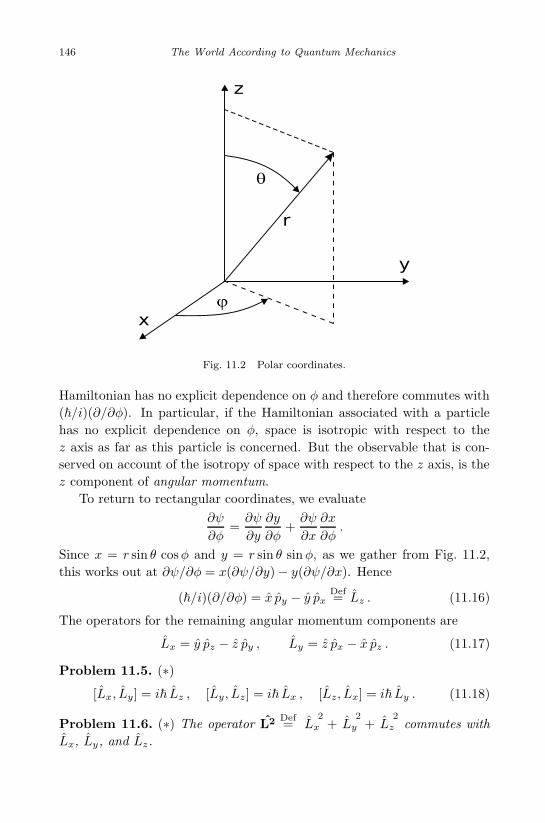
November 24, 2010 10:17 World Scientific Book - 9in x 6in main
146 The World According to Quantum Mechanics
Fig. 11.2 Polar coordinates.
Hamiltonian has no explicit dependence on φ and therefore commutes with
(~/i)(∂/∂φ). In particular, if the Hamiltonian associated with a particle
has no explicit dependence on φ, space is isotropic with respect to the
z axis as far as this particle is concerned. But the observable that is con-
served on account of the isotropy of space with respect to the z axis, is the
z component of angular momentum.
To return to rectangular coordinates, we evaluate
∂ψ
∂φ=∂ψ
∂y
∂y
∂φ+∂ψ
∂x
∂x
∂φ.
Since x = r sin θ cosφ and y = r sin θ sinφ, as we gather from Fig. 11.2,
this works out at ∂ψ/∂φ = x(∂ψ/∂y)− y(∂ψ/∂x). Hence
(~/i)(∂/∂φ) = x py − y pxDef= Lz . (11.16)
The operators for the remaining angular momentum components are
Lx = y pz − z py , Ly = z px − x pz . (11.17)
Problem 11.5. (∗)[Lx, Ly] = i~ Lz , [Ly, Lz] = i~ Lx , [Lz, Lx] = i~ Ly . (11.18)
Problem 11.6. (∗) The operator L2 Def= Lx
2+ Ly
2+ Lz
2commutes with
Lx, Ly, and Lz.

November 24, 2010 10:17 World Scientific Book - 9in x 6in main
Quantum mechanics resumed 147
11.8 The hydrogen atom in brief
Using the time-independent Schrodinger equation (4.25) with EP = −e2/r,we find—as one would expect from the discussion in Sec. 4.4—that bound
states exist only for specific values of E. These are exactly the values Bohr
obtained in 1913 (Eq. 2.7):
En = − 1
n2
me e4
2~2, n = 1, 2, 3, . . .
The influence of the electron on the proton can be taken into account by
substituting the reduced mass µ = mpme/(mp +me) for me, mp being the
proton’s mass.
If polar coordinates are used, factorizing ψ(r, φ, θ) into e(i/~) lzφ ψ(r, θ)
leads to a φ-independent Schrodinger equation and a discrete set of values
for lz, just as factorizing ψ(t, r) into e−(i/~) Et ψ(r) led to a t-independent
Schrodinger equation and a discrete set of values En. The φ-independent
Schrodinger equation contains a real parameter whose possible values are
given by l(l + 1)~2, where l is an integer satisfying the condition 0 ≤ l ≤n−1. The possible values of lz, in turn, are integers satisfying the inequality
|lz| ≤ l. The possible combinations of the quantum numbers n, l, lz are thus
n = 1 l = 0 lz = 0n = 2 l = 0 lz = 0
l = 1 lz = 0, ±1n = 3 l = 0 lz = 0
l = 1 lz = 0, ±1l = 2 lz = 0, ±1, ±2
......
...
The energy corresponding to the principal quantum number n is an eigen-
value of the Hamiltonian. The value l(l + 1)~2, where l is the angular
momentum (or orbital, or azimuthal) quantum number, is an eigenvalue of
L2. And the angular momentum component with respect to the z axis, ~ lz,
is an eigenvalue of Lz . lz is usually called the magnetic quantum number,
hence the letter m is often used instead. The eigenfunctions ψnlm(r, φ, θ)
of these operators form a complete set of bound-state solutions (E < 0) of
the Schrodinger equation for the hydrogen atom.
As “a picture is worth more than a thousand words” (and as the relevant
mathematics is set out in great detail in many textbooks), we content our-
selves with the illustrations on the following pages. States with l = 0, 1, 2, 3
were originally labeled s, p, d, f (for “sharp,” “principal,” “diffuse,” and
“fundamental”) with a view to characterizing the corresponding spectral
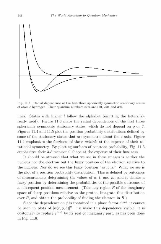
November 24, 2010 10:17 World Scientific Book - 9in x 6in main
148 The World According to Quantum Mechanics
Fig. 11.3 Radial dependence of the first three spherically symmetric stationary statesof atomic hydrogen. Their quantum numbers nlm are 1s0, 2s0, and 3s0.
lines. States with higher l follow the alphabet (omitting the letters al-
ready used). Figure 11.3 maps the radial dependences of the first three
spherically symmetric stationary states, which do not depend on φ or θ.
Figures 11.4 and 11.5 plot the position probability distributions defined by
some of the stationary states that are symmetric about the z axis. Figure
11.4 emphasizes the fuzziness of these orbitals at the expense of their ro-
tational symmetry. By plotting surfaces of constant probability, Fig. 11.5
emphasizes their 3-dimensional shape at the expense of their fuzziness.
It should be stressed that what we see in these images is neither the
nucleus nor the electron but the fuzzy position of the electron relative to
the nucleus. Nor do we see this fuzzy position “as it is.” What we see is
the plot of a position probability distribution. This is defined by outcomes
of measurements determining the values of n, l, and m, and it defines a
fuzzy position by determining the probabilities of the possible outcomes of
a subsequent position measurement. (Take any region R of the imaginary
space of sharp positions relative to the proton, integrate this distribution
over R, and obtain the probability of finding the electron in R.)
Since the dependence on φ is contained in a phase factor eimφ, it cannot
be seen in plots of |ψ(r, φ, θ)|2. To make this dependence visible, it is
customary to replace eimφ by its real or imaginary part, as has been done
in Fig. 11.6.

November 24, 2010 10:17 World Scientific Book - 9in x 6in main
Quantum mechanics resumed 149
Fig. 11.4 The position probability distributions associated with the following orbitals.First row: 2p0, 3p0, 3d0. Second row: 4p0, 4d0, 4f0. Third row: 5d0, 5f0, 5g0. Imagescreated with Orbital Viewer 1.04 by David Manthey.
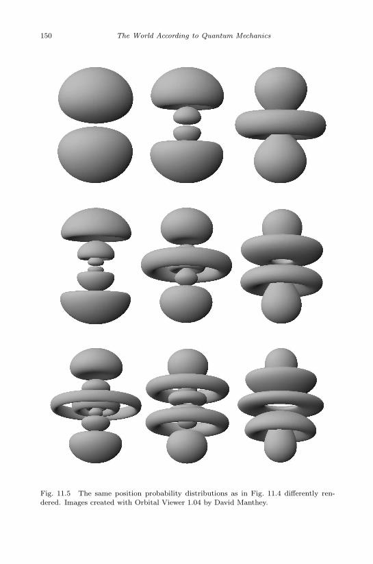
November 24, 2010 10:17 World Scientific Book - 9in x 6in main
150 The World According to Quantum Mechanics
Fig. 11.5 The same position probability distributions as in Fig. 11.4 differently ren-dered. Images created with Orbital Viewer 1.04 by David Manthey.

November 24, 2010 10:17 World Scientific Book - 9in x 6in main
Quantum mechanics resumed 151
Fig. 11.6 Orbitals with m 6= 0. The squares of their real parts are shown. First row:4f1, 5f1. Second row: 5f2, 5f3. Third row: 5g1, 5g3. Fourth row: 5g3, 5g4.

November 24, 2010 10:17 World Scientific Book - 9in x 6in main
This page intentionally left blankThis page intentionally left blank

December 23, 2010 10:25 World Scientific Book - 9in x 6in main
Chapter 12
Spin
12.1 Spin 1/2
In 1922, Otto Stern and Walther Gerlach found that when a narrow beam
of silver atoms is sent through an inhomogeneous magnetic field, it splits
into two beams. If the gradient of the magnetic field is oriented parallel
to the z axis (“upward”), and if the incoming beam runs parallel to the
y axis, then some atoms are deflected upward by a certain angle and the
rest are deflected downward by the same angle. The measurement of the
angle of deflection is repeatable: if the atoms in the upper (lower) beam
are made to pass through a second, identical apparatus, all of them are
deflected upward (downward).
Let the unit vectors |z+〉 and |z−〉 stand for the possible outcomes of
this measurement, in lieu of the projectors |z+〉〈z+| and |z−〉〈z−|. Repre-
senting different outcomes of the same measurement, the two vectors are
orthogonal, and corresponding to a complete set of possible outcomes, they
form a basis in a 2-dimensional vector space. For reasons that will soon
become clear, we refer to the property whose value is indicated by this
measurement as “the z component of the atom’s spin.”
The gradient of the magnetic field can of course point in any direction.
If it is parallel to the x axis, we are set to measure the x component of
the atom’s spin. Its possible values are represented by the vectors |x+〉 and|x−〉. A different complete set of mutually orthogonal unit vectors, they
form another basis in this 2-dimensional space of spin states. By Born’s
rule, the probability of obtaining the outcome |z+〉 after having obtained
the outcome |x+〉 (and made sure that no external influence has affected
the probabilities of the possible outcomes in the meantime) is |〈z+|x+〉|2.
153

November 24, 2010 10:17 World Scientific Book - 9in x 6in main
154 The World According to Quantum Mechanics
According to a common phraseology, the first measurement prepares the
atom in the state |x+〉, with the result that subsequently the atom is in
this state. Expressions of this sort are seriously misleading. For one thing,
a quantum state is a probability algorithm, and a physical system cannot
be “in” a probability algorithm.
Let us send the atoms in the upper beam through an apparatus that is
identical to the first except that it is rotated by an angle α about the z axis.
We shall denote by |z′′+〉 and |z′′−〉 the possible outcomes of a measurement
made with this apparatus. Since the two apparatuses measure the same spin
component, the probabilities |〈z′′+|z+〉|2 and |〈z′′−|z−〉|2 are equal to unity,
and the probabilities |〈z′′−|z+〉|2 and |〈z′′+|z−〉|2 are zero. The amplitude
〈z′′+|z+〉 is thereby determined up to a phase factor.
Problem 12.1. (∗) If 〈z′′+|z+〉 = eiφ then |z′′+〉 = e−iφ|z+〉.
Our next move is to interpose a third measurement of the z component of
the atom’s spin, using an apparatus that is rotated relative to the first by
an angle α/2 about the z axis. The corresponding outcomes are |z ′+〉 and
|z′−〉. If this intermediate measurement is not made, then by Rule B we
have that
〈z′′+|z+〉 = 〈z′′+|z′+〉〈z′+|z+〉+ 〈z′′+|z′−〉〈z′−|z+〉 . (12.1)
But we also have that |〈z′−|z+〉|2 = |〈z′′+|z′−〉|2 = 0. This leaves us with
〈z′′+|z+〉 = 〈z′′+|z′+〉〈z′+|z+〉 or
eiφ(α) = eiφ(α/2)eiφ(α/2). (12.2)
Since the right-hand side equals ei 2φ(α/2), φ is proportional to α: 〈z′′+|z+〉 =eibα. By the same token, 〈z′′−|z−〉 = eib′α. Because overall phase factors lack
physical significance—for at the end of the day we are left with absolute
squares of sums of amplitudes—we can see to it that
|z′′+〉 = e−ilα|z+〉, |z′′−〉 = eilα|z−〉 . (12.3)
What do we know about the value of l? For one thing, it cannot be zero.
Every vector in the space of spin states is a linear combination of |z+〉and |z−〉. If these two vectors are not affected by a rotation about the
z axis—i.e., if |z′′+〉 = |z+〉 and |z′′−〉 = |z−〉—then no vector is affected, nor
are the probabilities of outcomes of spin measurements with respect to the
x and y axes changed. But these probabilities ought to be changed by a
rotation about the z axis.
Nor can l be equal to unity, for if it were, a rotation by π about the
z axis would change the signs of |z+〉 and |z−〉 and, consequently, those of
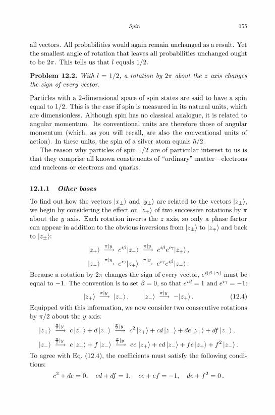
November 24, 2010 10:17 World Scientific Book - 9in x 6in main
Spin 155
all vectors. All probabilities would again remain unchanged as a result. Yet
the smallest angle of rotation that leaves all probabilities unchanged ought
to be 2π. This tells us that l equals 1/2.
Problem 12.2. With l = 1/2, a rotation by 2π about the z axis changes
the sign of every vector.
Particles with a 2-dimensional space of spin states are said to have a spin
equal to 1/2. This is the case if spin is measured in its natural units, which
are dimensionless. Although spin has no classical analogue, it is related to
angular momentum. Its conventional units are therefore those of angular
momentum (which, as you will recall, are also the conventional units of
action). In these units, the spin of a silver atom equals ~/2.
The reason why particles of spin 1/2 are of particular interest to us is
that they comprise all known constituents of “ordinary” matter—electrons
and nucleons or electrons and quarks.
12.1.1 Other bases
To find out how the vectors |x±〉 and |y±〉 are related to the vectors |z±〉,we begin by considering the effect on |z±〉 of two successive rotations by π
about the y axis. Each rotation inverts the z axis, so only a phase factor
can appear in addition to the obvious inversions from |z±〉 to |z∓〉 and back
to |z±〉:
|z+〉π|y−→ eiβ |z−〉
π|y−→ eiβeiγ |z+〉 ,
|z−〉π|y−→ eiγ |z+〉
π|y−→ eiγeiβ |z−〉 .Because a rotation by 2π changes the sign of every vector, ei(β+γ) must be
equal to −1. The convention is to set β = 0, so that eiβ = 1 and eiγ = −1:
|z+〉π|y−→ |z−〉 , |z−〉
π|y−→ −|z+〉 . (12.4)
Equipped with this information, we now consider two consecutive rotations
by π/2 about the y axis:
|z+〉π
2|y−→ c |z+〉+ d |z−〉
π
2|y−→ c2 |z+〉+ cd |z−〉+ de |z+〉+ df |z−〉 ,
|z−〉π
2|y−→ e |z+〉+ f |z−〉
π
2|y−→ ec |z+〉+ ed |z−〉+ fe |z+〉+ f2 |z−〉 .
To agree with Eq. (12.4), the coefficients must satisfy the following condi-
tions:
c2 + de = 0, cd+ df = 1, ce+ ef = −1, de+ f 2 = 0 .

November 24, 2010 10:17 World Scientific Book - 9in x 6in main
156 The World According to Quantum Mechanics
The first and the last condition imply that f = c or f = −c. The second
condition pins it down to f = c and yields d = 1/2c, and the third condition
yields e = −1/2c. With these results, the first condition tells us that
c4 = 1/4, which has four solutions. We are free to choose c = 1/√
2, and
this gives us
|z+〉π
2|y−→ 1√
2
[
|z+〉+ |z−〉]
, |z−〉π
2|y−→ 1√
2
[
−|z+〉+ |z−〉]
. (12.5)
12.1.2 Rotations as 2 × 2 matrices
Our next task will be to cast these rotations into matrix notation. If |1〉and |2〉 make up a basis, any vector can be written in the form
|a〉 = a1|1〉+ a2|2〉 , (12.6)
and any linear operator A can be given the form
A = A11|1〉〈1|+A12|1〉〈2|+A21|2〉〈1|+ A22|2〉〈2| . (12.7)
Applying A to |a〉 (from the left), or inserting |a〉 into A (from the right),
and making use of the orthonormality conditions (8.9), we obtain
|b〉 Def= A|a〉 = (A11a1 +A12a2)|1〉+ (A21a1 +A22a2)|2〉 . (12.8)
Here is the same equation in matrix notation:(b1b2
)
=
(A11 A12
A21 A22
)(a1
a2
)
=
(A11a1 +A12a2
A21a1 +A22a2
)
. (12.9)
It is just another way of writing bi =∑2
k=1 Aikak for i = 1, 2. (It would not
have escaped your notice that the dependence of the components of vectors
and matrices on a particular basis is no longer explicit in this notation.)
Problem 12.3. Aik = 〈i|A|k〉.
Problem 12.4. (∗) 〈i|A†|k〉 = A∗ki.
Problem 12.5. (∗) The first column of the matrix representation of A
contains the components of A|1〉, the second those of A|2〉.
With respect to the |z±〉 basis, a rotation by π about the y axis (Eq. 12.4)
is effected by
R(π|y) =
(0 −1
1 0
)
, (12.10)

November 24, 2010 10:17 World Scientific Book - 9in x 6in main
Spin 157
while a rotation by π/2 about the y axis (Eq. 12.5) is effected by
R(
π2 |y)
=
(1/√
2 −1/√
2
1/√
2 1/√
2
)
. (12.11)
Problem 12.6. (∗) Cast the transformation (6.43) into matrix notation.
The multiplication of two N × N matrices A, B yields an N × N matrix
C = A · B whose components are defined by Cik =∑N
j=1 AijBjk . Note
that matrices don’t commute: in general, A · B 6= B · A.
Problem 12.7. (∗) In terms of matrix components, Eq. (8.38) reads
N∑
j=1
U∗ji Ujk = δik . (12.12)
Problem 12.8. The matrices (12.10) and (12.11) satisfy
R(
π2 |y)· R(
π2 |y)
= R(π|y) . (12.13)
Here is the upshot of Sec. 12.1 in matrix notation:
R (α|z) =
(e−iα/2 0
0 eiα/2
)
. (12.14)
Problem 12.9. R(α|z) · R(α|z) = R(2α|z).
The isotropy of space argues (i) that this holds for any axis, and (ii) that
for any axis,
R(2π) =
(−1 0
0 −1
)
. (12.15)
Problem 12.10. The matrices (12.10) and (12.15) satisfy
R(π|y) · R(π|y) = R(2π) . (12.16)
Problem 12.11.
R(
32π|y
)=
(−1/√
2 −1/√
2
1/√
2 −1/√
2
)
. (12.17)
One does not have to look far to find the right continuous functions of α
that reproduce the components of the matrices (12.10), (12.11), (12.15),
and (12.17):
R (α|y) =
(cos(α/2) − sin(α/2)
sin(α/2) cos(α/2)
)
. (12.18)
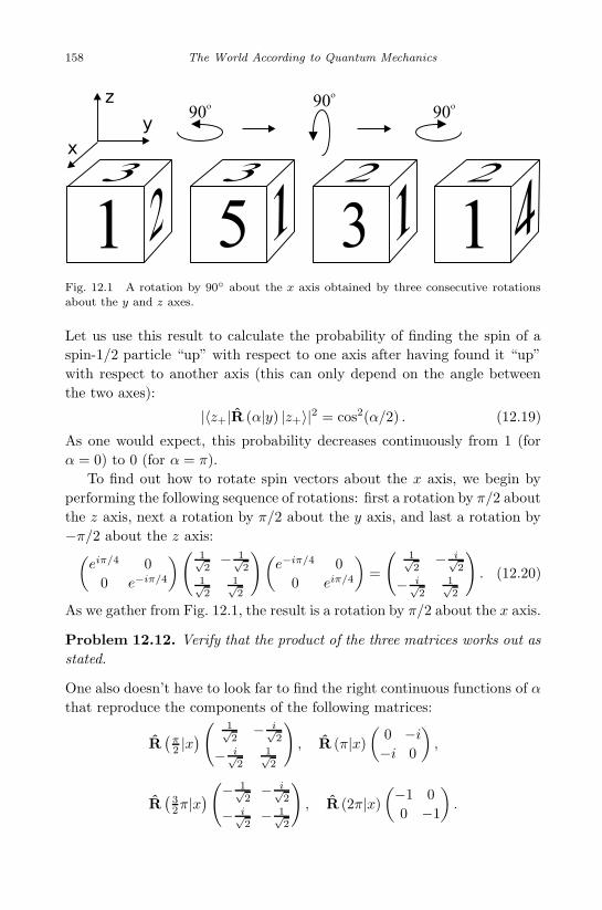
November 24, 2010 10:17 World Scientific Book - 9in x 6in main
158 The World According to Quantum Mechanics
Fig. 12.1 A rotation by 90◦ about the x axis obtained by three consecutive rotationsabout the y and z axes.
Let us use this result to calculate the probability of finding the spin of a
spin-1/2 particle “up” with respect to one axis after having found it “up”
with respect to another axis (this can only depend on the angle between
the two axes):
|〈z+|R (α|y) |z+〉|2 = cos2(α/2) . (12.19)
As one would expect, this probability decreases continuously from 1 (for
α = 0) to 0 (for α = π).
To find out how to rotate spin vectors about the x axis, we begin by
performing the following sequence of rotations: first a rotation by π/2 about
the z axis, next a rotation by π/2 about the y axis, and last a rotation by
−π/2 about the z axis:(eiπ/4 0
0 e−iπ/4
)( 1√2− 1√
2
1√2
1√2
)(e−iπ/4 0
0 eiπ/4
)
=
(1√2− i√
2
− i√2
1√2
)
. (12.20)
As we gather from Fig. 12.1, the result is a rotation by π/2 about the x axis.
Problem 12.12. Verify that the product of the three matrices works out as
stated.
One also doesn’t have to look far to find the right continuous functions of α
that reproduce the components of the following matrices:
R(
π2 |x)
(1√2− i√
2
− i√2
1√2
)
, R (π|x)(
0 −i−i 0
)
,
R(
32π|x
)
(− 1√2− i√
2
− i√2− 1√
2
)
, R (2π|x)(−1 0
0 −1
)
.

November 24, 2010 10:17 World Scientific Book - 9in x 6in main
Spin 159
Here they are:
R (α|x) =
(cos(α/2) −i sin(α/2)
−i sin(α/2) cos(α/2)
)
. (12.21)
We are now in a position to define the basis vectors with respect to the
x and y axes by rotating |z+〉 by the appropriate angle (+π/2 or −π/2)
about the appropriate axis:
|x+〉 = R(
π2 |y)|z+〉 =
1√2
[
|z+〉+ |z−〉]
, (12.22)
|y+〉 = R(−π
2 |x)|z+〉 =
1√2
[
|z+〉+ i|z−〉]
, (12.23)
|x−〉 = R(−π
2 |y)|z+〉 =
1√2
[
|z+〉 − |z−〉]
, (12.24)
|y−〉 = R(
π2 |x)|z+〉 =
1√2
[
|z+〉 − i|z−〉]
. (12.25)
12.1.3 Pauli spin matrices
Which self-adjoint operators correspond to the three spin components of
a spin-1/2 particle? The eigenvectors of these operators are |x±〉, |y±〉,and |z±〉, respectively, while the corresponding eigenvalues are ±1/2 (in
natural units) or ±~/2 (in conventional units). If we take the eigenvalues
to be ±1 (for “up” and “down”), the wanted operators—in matrix notation
with respect to the basis |z±〉—are the Pauli matrices :
σx =
(0 1
1 0
)
, σy =
(0 −ii 0
)
, σz =
(1 0
0 −1
)
. (12.26)
Problem 12.13.
σx|x±〉 = ±|x±〉 , σy|y±〉 = ±|y±〉 , σz |z±〉 = ±|z±〉 . (12.27)
Problem 12.14.
σxσx = σyσy = σzσz = −iσxσyσz = 1Def=
(1 0
0 1
)
. (12.28)
Problem 12.15.
σxσy = iσz, σyσz = iσx, σzσx = iσy . (12.29)
Problem 12.16. (∗)[σx, σy] = 2iσz , [σy, σz ] = 2iσx , [σz , σx] = 2iσy . (12.30)

November 24, 2010 10:17 World Scientific Book - 9in x 6in main
160 The World According to Quantum Mechanics
When we introduced the commutator of two operators (Sec. 11.4), we con-
cluded that measurements of the corresponding observables are compatible
if and only if the operators commute. Since the operators corresponding
to different components of the same spin do not commute, different com-
ponents of the same spin are incompatible. There is no state that assigns
probability 1 to possible outcomes of measurements of more than one spin
component.
For later use we record the general form of a rotation by α about an axis
defined by the unit vector n = (nx, ny, nz) [Marchildon (2002), Sec. 4.6]:
R(α|n) =
(cos(α/2)− inz sin(α/2) −(inx + ny) sin(α/2)
(−inx + ny) sin(α/2) cos(α/2) + inz sin(α/2)
)
= exp(
−iα2
n · σ)
.
The components of σ are the Pauli matrices (12.26), and the exponential is
defined by its Taylor expansion. A further streamlining of the notation is
achieved by introducing the vector α = αn and by defining s = σ/2. This
allows us to write
R(α) = e−i α·s. (12.31)
In terms of the components of s, the commutators (12.30) take the form
[sa, sb ] = iεabcsc , (12.32)
where
εabc =
+1 if abc is an even permutation of xyz
−1 if abc is an odd permutation of xyz
0 if abc is not a permutation of xyz
(12.33)
12.2 A Stern–Gerlach relay
A beam of spin-1/2 atoms passes through three inhomogeneous magnetic
fields (from the right to the left as in Fig. 12.2). The gradients in the first
and the third magnet point upward (toward the tip of the upper pole, where
the field is strongest), while the gradient in the second magnet points to
the right (relative to the atom’s direction of motion). Unless the atoms are
specially prepared, the beam gets split three times: first into two beams
that are deflected upward and downward, respectively, then into four beams
two of which are deflected to the left and two to the right, and finally into
eight beams, four of which are deflected upward and four downward. We
thus expect the atoms to hit the screen in eight spots.

November 24, 2010 10:17 World Scientific Book - 9in x 6in main
Spin 161
Fig. 12.2 The apparatus used in Sec. 12.2.
What happens if we gradually reduce the power of the second magnet,
so that the four left spots first overlap and then merge with the four right
spots? How many spots will be seen?
Let us calculate, assuming that initially the pure state |a〉 is associated
with each atom. The amplitude for an atom’s arrival in the uppermost
right spot (with respect to the atom’s direction of motion) is
〈z+|x+〉〈x+|z+〉〈z+|a〉 =1
2〈z+|a〉 . (12.34)
Problem 12.17. (∗) The probability of an atom’s arrival at the screen (no
matter at which spot) equals 1.
If the second magnet is switched off, the amplitude for an atom’s arrival at
the (now single) uppermost spot is
〈z+|x+〉〈x+|z+〉〈z+|a〉+ 〈z+|x−〉〈x−|z+〉〈z+|a〉 = 〈z+|a〉 , (12.35)
whereas the amplitude for an atom’s arrival at the (now single) spot directly
below is
〈z−|x+〉〈x+|z+〉〈z+|a〉+ 〈z−|x−〉〈x−|z+〉〈z+|a〉 = 0 . (12.36)
By the same token, the amplitude for an atom’s arrival at the (now single)
lowermost spot is 〈z−|a〉, whereas the amplitude for an atom’s arrival at the
(now single) spot directly above is 0. The reason why the atoms arrive in
two spots rather than four is this: without the intermediate measurement
of the x component, the repeatability of measurements guarantees that
the outcome of the second measurement of the z component confirms the
outcome of the first measurement. Figure 12.3 illustrates what happens if
the power of the second magnet is gradually reduced.

December 23, 2010 10:25 World Scientific Book - 9in x 6in main
162 The World According to Quantum Mechanics
Fig. 12.3 Constructive or destructive interference occurs in regions where the outcomeof the measurement of the spin’s x component is no longer indicated.
12.3 Why spin?
This makes two questions: Why is it called “spin”? And what is it for?
In answer to the first question, we observe that wave functions trans-
forming under rotations about the z axis as ψ −→ eimφψ are eigenstates
of Lz with eigenvalue m, while spin states transforming under rotations
about this axis as |s〉 −→ eiφ/2|s〉 are eigenstates of σz with eigenvalue 1/2.
Both angular momentum and spin—also called extrinsic and intrinsic an-
gular momentum, respectively—are conserved for closed systems because
the Hamiltonians of such systems reflect the isotropy of space (in this par-
ticular case, with respect to rotations about the z axis).
And what is it for? The answer to this question emerges from one of
those theorems that are as easy to state as they are hard to prove [Pauli
(1940); Duck and Sudarshan (1998)]. Particle beams passing through an
inhomogeneous magnetic field may split into b = 2, 3, 4, . . . beams depend-
ing on the particles’ spin. Beams consisting of spinless particles, for which
l = 0, don’t split. Beams consisting of spin-1/2 particles split into two
beams, as we have seen. The general rule is b = 2 l+ 1, where the possible
values of l are 0, 1, 2, 3 . . . and 1/2, 3/2, 5/2 . . . .
As we shall see in Sec. 14.2, every particle is either a boson or a fermion.
The aforementioned theorem, due to Pauli, states that a fermion cannot
have an integral spin (l = 0, 1, 2, . . . ), whereas a boson cannot have a half-
integral spin (l = 1/2, 3/2, 5/2, . . .). But only fermions obey the exclusion
principle (Sec. 14.5), and the stability of matter requires that its fundamen-
tal constituents—electrons and nucleons or electrons and quarks—obey this

November 24, 2010 10:17 World Scientific Book - 9in x 6in main
Spin 163
principle (see Sec. 22.1). The long and the short of it is that the funda-
mental constituents of matter must be particles with a half-integral spin of
at least 1/2.
12.4 Beyond hydrogen
The helium atom has two electrons, and its nucleus—two protons and two
neutrons—has about four times the mass of the hydrogen nucleus. If the in-
fluence of the electrons on the nucleus as well as relativistic and spin effects
are ignored, the corresponding stationary states are in principle obtainable
as solutions of the following equation:
E∂ψ
∂t=− ~
2
2m
[∂2ψ
∂x21
+∂2ψ
∂y21
+∂2ψ
∂z21
+∂2ψ
∂x22
+∂2ψ
∂y22
+∂2ψ
∂z22
]
+
[
−2e2
r1− 2e2
r2+
e2
r12
]
ψ . (12.37)
The wave function now depends on the six coordinates x1, y1, z1, x2, y2, z2of the two electrons relative to the nucleus, and the potential energy is
made up of three terms: two that are inverse proportional to the respective
distances r1 =√
x21 + y2
1 + z21 and r2 =
√
x22 + y2
2 + z22 between the elec-
trons and the nucleus, and one that is inverse proportional to the distance
r12 =√
(x2−x1)2 + (y2−y1)2 + (z2−z1)2 between the electrons.
The fact that we have one wave function depending on six coordinates
rather than two separate wave functions each depending on three coordi-
nates, should not come as a surprise. The sole purpose of wave functions
depending on more than one coordinate is to let us calculate joint prob-
abilities, which may be correlated (Sec. 1.4). The probability of finding
the first electron in a region A and the second electron in a region B, for
example, is given by the joint probability
p(A,B) =
∫
A
d3r1
∫
B
d3r2 |ψ(r1, r2)|2. (12.38)
If the whereabouts of the two electrons were independent of each other, it
would be possible to factorize ψ(r1, r2) into ψ1(r1) and ψ2(r2), and p(A,B)
would be the product of the probabilities
p(A) =
∫
A
d3r1 |ψ(r1)|2, p(B) =
∫
B
d3r2 |ψ(r2)|2.

November 24, 2010 10:17 World Scientific Book - 9in x 6in main
164 The World According to Quantum Mechanics
But in general, and particularly where the solutions of Eq. (12.37) are
concerned, this is not the case.
For the lowest energy levels, Eq. (12.37) has been solved by numerical
methods. With three or more electrons in the picture, looking for exact
solutions of the corresponding Schrodinger equation is a hopeless under-
taking. Through further simplifications it is nevertheless possible to get
valuable results. The Periodic Table and many properties of the chemical
elements can be understood by using the central field approximation [e.g.,
Marchildon (2002), Sec. 9.3]. In this approach, one disregards the details
of the interactions between electrons. One instead considers each electron
subject to two potentials, one representing the effect of the nucleus, and
one representing the effect of a continuous, spherically symmetric charge
distribution, which does duty for the remaining electrons. Spin effects are
also neglected except for the Pauli exclusion principle (Sec. 14.5), which
implies that two electrons associated with the same wave function cannot
be also associated with the same spin state. Measurements of their spin
components with respect to the same axis—no matter which—will yield
different outcomes. Because only two outcomes are possible, at most two
electrons can share the same orbital.
The central field approximation yields stationary wave functions
ψnlm(r) for single electrons that are quite similar to those of atomic hydro-
gen, except that their dependence on the radial coordinate is modified by
the charge distribution that stands in for the other electrons. This modi-
fication has the result that the energies associated with orbitals with the
same quantum number n but with different quantum numbers l are no
longer equal. For any n > 1, the mean distance between the electron and
the nucleus increases with l. With a greater mean distance, the electron is
more shielded against the nucleus by the cloud of negative charge represent-
ing the other electrons. Electrons with higher l are therefore less strongly
bound and their ionization energies are lower.
Problem 12.18. The number of orbitals with the same quantum number n
is n2.
Chemists group orbitals into electron shells. Each shell encompasses all
orbitals with the same principal quantum number n. The nth shell can
therefore “accommodate” 2 × n2 electrons—twice n2 because each orbital
can “accommodate” two electrons.
Helium has a “full” first shell and an “empty” second shell. Because
the helium nucleus has twice the charge of the hydrogen nucleus, the two

November 24, 2010 10:17 World Scientific Book - 9in x 6in main
Spin 165
electrons are, on average, significantly closer to the nucleus than the single
electron of the hydrogen atom. The ionization energy of helium, accord-
ingly, is much higher, 24.6 eV as compared to 13.6 eV. On the other hand, if
we tried to add an electron to create a negative helium ion, this would have
to “go into” the second shell, which is strongly shielded from the nucleus
by the electrons of the first shell. Helium is therefore neither prone to give
up an electron not able to hold on to an extra electron. It is chemically
inert, as are all of the elements in the rightmost column of the (traditional)
Periodic Table.
Through the second row of the Periodic Table, the second shell gets
“filled.” Because the energies of the 2p orbitals are higher than the energy
of the 2s orbital, the latter gets “occupied” first. With each added electron
(and proton) the electron distribution as a whole gets pulled inward, and
the ionization energy goes up, from 5.4 eV for lithium (atomic number
Z=3) to 21.6 eV for neon (Z=10). Whereas lithium readily parts with
its loosely bound outer electron, fluorine (Z=9), having a single “vacancy”
in the second shell, is eager to grab one. Both are therefore quite active
chemically. The progression from sodium (Z=11) to argon (Z=18) parallels
that from lithium to neon.
There is a noteworthy peculiarity in this progression of ionization ener-
gies: the ionization energy of oxygen (Z=8, 13.6 eV) is lower than that of
nitrogen (Z=7, 14.5 eV), and that of sulfur (Z=16, 10.36 eV) is lower than
that of phosphorus (Z=15, 10.49 eV). To understand why this is so, we
must take account of certain details that have so far been ignored. Suppose
that one of the two 2p electrons of carbon (Z=6) goes into the m=0 orbital
(with respect to the z axis). Where will the other 2p electron go? It will
go into any “vacant” orbital that minimizes the repulsion between the two
electrons by maximizing their mean distance. This is neither of the two
orbitals with |m|=1 with respect to the z axis but an orbital with m=0
with respect to some axis perpendicular to the z axis. If we call this the
x axis, then the third 2p electron of nitrogen goes into the orbital with m=0
relative to y axis. The fourth 2p electron of oxygen then has no choice but
to go into an already occupied 2p orbital. This raises its energy sufficiently
for the drop in ionization energy from nitrogen to oxygen.
By the time the 3p orbitals are completely “filled,” the energies of the
3d states are pushed up so high (as a result of shielding) that the 4s state
is energetically lower. The “filling” up of the 3d orbitals therefore begins
only after the 4s orbitals are “full,” with scandium (Z=21).

November 24, 2010 10:17 World Scientific Book - 9in x 6in main
166 The World According to Quantum Mechanics
12.5 Spin precession
The Pauli equation (15.6) is to a non-relativistic particle of spin 1/2 what
the Schrodinger equation (7.23) is to a non-relativistic particle without spin.
The Pauli wave function has two components, and what interests us here
is how they depend on each other:
i~d
dt
(ψ+
ψ−
)
= −µ σ ·B(ψ+
ψ−
)
=
( −µBz −µ(Bx − iBy)
−µ(Bx + iBy) µBz
)(ψ+
ψ−
)
.
B is the magnetic field, and if q and m are the charge and mass of an elec-
tron, then µ = q~/2mc is the Bohr magneton. If the particle is subject to
a homogeneous magnetic field B = (0, 0, B), the two equations are actually
independent of each other:
i~dψ+
dt= −µBψ+ , i~
dψ−dt
= +µBψ− .
Their respective solutions are proportional to e±(i/~)µBt, and they predict
the respective outcomes ±µB for a measurement of the energy associated
with the electron’s spin. If instead B = (B, 0, 0), we obtain the coupled
equations
i~dψ+
dt= −µBψ− , i~
dψ−dt
= −µBψ+ .
A possible pair of solutions is
ψ+ = cos
(µB
~t
)
, ψ− = i sin
(µB
~t
)
.
This tells us that the probabilities associated with a measurement of the
z component of the spin, pz+ and pz
−, oscillate as follows:
pz+ = cos2
(µB
~t
)
, pz− = sin2
(µB
~t
)
= cos2(µB
~t± π
2
)
. (12.39)
To find out how the probabilities py+ and py
− associated with a measure-
ment of the y component of the spin oscillate, we make use of Eqs. (12.23)
and (12.25):
ψy+ =
1√2
(ψ+ + iψ−
)
=1√2
[
cos
(µB
~t
)
− sin
(µB
~t
)]
= cos
(µB
~t+
π
4
)
,
ψy− =
1√2
(ψ+ − iψ−
)
=1√2
[
cos
(µB
~t
)
+ sin
(µB
~t
)]
= cos
(µB
~t− π
4
)
.

November 24, 2010 10:17 World Scientific Book - 9in x 6in main
Spin 167
Hence,
py+ = cos2
(µB
~t+
π
4
)
, py− = cos2
(µB
~t− π
4
)
. (12.40)
From Eqs. (12.39) and (12.40) we gather that the axis with respect to
which a spin measurement yields “up” with probability 1 is precessing at
the frequency ω = 2µB/~. (Bear in mind that the period of cos2 is π.)
12.6 The quantum Zeno effect
Consider a spin that is precessing about the x axis as described in the
previous section. At t = 0, the probability of finding it up with re-
spect to the z axis equals 1. At later times, this probability is given by
p(t) = cos2(µBt/~). If we measure the z component of the spin N times at
intervals of duration t/N , the probability of finding it up each time equals
[p(t/N)]N =[cos2(µBt/N~)
]N. (12.41)
As N → ∞, this tends to unity. A finite number of (instantaneous) mea-
surements slows down the precession, and an infinite number of measure-
ments performed during a finite interval would bring it to a halt.
While no measurement is instantaneous and the limit N →∞ is physi-
cally unattainable, the tendency of repeated measurements to slow down the
rate at which the probabilities of the possible outcomes change, is a general
and experimentally well-established feature of quantum mechanics [Misra
and Sudarshan (1977); Peres (1980); Singh and Whitaker (1982)]. The ef-
fect is named after the Eleatic philosopher Zeno who, in the 5th Century
B.C.E., put forth a series of apparent paradoxes designed to demonstrate
that motion was impossible.
The reverse effect also exists. If there is no magnetic field and the
spin is measured at intervals of duration t/N with respect to an axis that
rotates with angular frequency ω about the x axis, the probability of find-
ing it up each time is again given by Eq. (12.41). In this case, a finite
number of (instantaneous) measurements causes a certain amount of pre-
cession, and in the unphysical limit N → ∞ this approaches the angular
frequency of the rotating apparatus. This too is a general and experimen-
tally well-established feature of quantum mechanics. If an infinite number
of measurements could be performed during a finite interval, the behavior
of a quantum system would be determined exclusively by what the experi-
menters chose to measure.

November 24, 2010 10:17 World Scientific Book - 9in x 6in main
168 The World According to Quantum Mechanics
The bottom line: for the quantum-mechanical correlation laws to be
effective, not only must there be measurements (whose possible outcomes
they serve to correlate) but also there must be unmeasured intervals be-
tween the measurements.

November 24, 2010 10:17 World Scientific Book - 9in x 6in main
Chapter 13
Composite systems
13.1 Bell’s theorem: The simplest version
Consider the following setup [Mermin (1985)] (Fig. 13.1):
Fig. 13.1 Mermin’s simplest version of Bell’s theorem.
The device at the center launches two particles in opposite directions. Each
particle enters an apparatus capable of performing one of three measure-
ments. Each measurement has two possible outcomes, indicated by a red
or green light. In each run of the experiment the measurement performed
is randomly selected for each apparatus. After a large number of runs, we
have in our hands a long record of apparatus settings and responses. This
record has the following characteristics:
• Whenever both apparatuses perform the same measurement (11, 22, or
33), equal colors (RR or GG) are never observed.
• The pattern of R’s and G’s is completely random.
In particular, the apparatuses flash different colors exactly half of the time.
If this does not bother you, then try to explain how it is that the colors
differ whenever identical measurements are performed!
The obvious explanation is that each particle arrives with an “instruc-
tion set”—a set of properties determining how the apparatus will respond.
169

December 23, 2010 10:25 World Scientific Book - 9in x 6in main
170 The World According to Quantum Mechanics
There are 23 = 8 such sets: RRR, RRG, RGR, GRR, RGG, GRG, GGR,
and GGG. If, for instance, a particle arrives with RGG, the apparatus
flashes red if it is set to 1, and green if it is set to 2 or 3. According to this
explanation, the reason why the outcomes differ whenever both particles are
subjected to the same measurement is that the particles are launched with
opposite instruction sets. If one particle carries the instruction set RRG,
then the other particle carries the instruction set GGR.
Let us see if this explanation is tenable. Suppose that the instruction
sets are RRG and GGR. In this case we expect to see different colors with
five of the 32 = 9 possible combinations of apparatus settings (namely,
11, 22, 33, 12, 21) and to see equal colors with four of them (namely, 13,
23, 31, and 32). Because the apparatus settings are randomly chosen, this
pair of instruction sets produces different colors 5/9 of the time. The same
is obviously true for the remaining pairs of instruction sets except the pair
RRR, GGG. If the two particles carry these instruction sets, we see different
colors every time, irrespective of the apparatus settings. If follows that we
see different colors at least 5/9 of the time. The probability of observing
different colors is greater than 5/9. This is Bell’s inequality for the present
setup.
If the particles did arrive with instruction sets—i.e., if each particle did
come with three properties the possession of any one of which is revealed by
the apparatus—then Bell’s inequality would be satisfied. But it isn’t, since
the apparatuses flash different colors half of the time. We appear forced to
conclude, in this instance as in many similar experimental situations, that
the predictions of quantum mechanics cannot be explained with the help of
instruction sets [Aspect (2002); Greenstein and Zajonc (1997); Laloe (2001);
Redhead (1987)]. These measurements do not reveal pre-existent properties
or values. In a radical sense, they create their outcomes. They create the
properties or values whose possession (by a system or an observable) they
indicate.
But then how is it that the colors differ whenever identical measurements
are made? Since each apparatus indicates each possible outcome half of the
time, the marginal probabilities of the outcomes are p(R) = p(G) = 1/2. If
the outcomes were uncorrelated, we would have that p(R,G) = p(G,R) =
p(R,R) = p(G,G) = 1/4. Instead we have p(R,R) = p(G,G) = 0 and
p(R,G) = p(G,R) = 1/2 whenever the apparatus settings agree. What
mechanism or process is responsible for these correlations? How does one
apparatus or particle “know” which measurement is performed and which
outcome is obtained by the other apparatus? I can tell you the answer

November 24, 2010 10:17 World Scientific Book - 9in x 6in main
Composite systems 171
straight off: you understand this as well as anybody else! As a distinguished
Princeton physicist commented, “anybody who’s not bothered by Bell’s
theorem has to have rocks in his head” [quoted by Mermin (1985)].
Einstein was bothered, albeit not by Bell’s theorem, whose original
version [Bell (1964)] appeared several years after his death. The title of
Bell’s 1964 paper, “On the Einstein Podolsky Rosen paradox,” refers to
a seminal paper of 1935, in which Einstein, Podolsky, and Rosen made
use of similar correlations—now often collectively referred to as “EPR cor-
relations”—to argue that quantum mechanics was incomplete. In 1947,
Einstein wrote in a letter to Max Born that he could not seriously be-
lieve in the quantum theory “because it cannot be reconciled with the idea
that physics should represent a reality in time and space, free from spooky
actions at a distance” [Einstein (1971)]. In his 1964 paper, Bell was led
to conclude that, on the contrary, “there must be a mechanism whereby
the setting of one measurement device can influence the reading of another
instrument, however remote.” Spooky actions at a distance are here to
stay! As Bell wrote in a subsequent paper [Bell (1966)], “the Einstein–
Podolsky–Rosen paradox is resolved in a way which Einstein would have
liked least.”
13.2 “Entangled” spins
Consider two physical systems A and B, which have been subjected to mea-
surements. The respective outcomes are |a〉〈a| and |b〉〈b|. If no interactions
take place between the systems—which could lead to correlations between
the outcomes of subsequent measurements—then the systems remain as-
sociated with vectors |a(t)〉 and |b(t)〉 belonging to the respective vector
spaces Va and Vb of the individual systems. In this case the composite sys-
tem made up of A and B is associated with the pair of vectors |a(t)〉 and
|b(t)〉, which is itself a vector. This vector—denoted by |a(t)〉 ⊗ |b(t)〉 or,
more simply, by |a, b (t)〉—belongs to the vector space Va ⊗ Vb, the direct
product of the two vector spaces.
The scalar product in Va⊗Vb is the product of two scalar products, one
in Va and one in Vb:
〈a′, b′|a, b〉 = 〈a′|a〉 〈b′|b〉 . (13.1)
If the vectors |a1〉, . . . , |am〉 form a basis in Va and the vectors |b1〉, . . . , |bn〉form a basis in Vb, then the mn vectors |ai, bk〉 form a basis in Va ⊗ Vb .

November 24, 2010 10:17 World Scientific Book - 9in x 6in main
172 The World According to Quantum Mechanics
Given a composite system associated with the vector |a, b〉, the proba-
bility of obtaining the respective outcomes |a′〉〈a′| and |b′〉〈b′| thus equals
|〈a′, b′|a, b〉|2 = |〈a′|a〉|2 |〈b′|b〉|2. (13.2)
This is what we expect on the basis of Born’s rule, and what motivates the
above definitions in the first place.
Most vectors in Va ⊗ Vb cannot be written as a single pair of vectors,
and this is where it gets interesting. In such cases the outcomes of at least
some of the measurements that can be performed on the component systems
are correlated, and the component systems are said to be entangled. It is,
however, always possible to find a pair of bases—say, |Ai〉 in Va and |Bj〉in Vb—such that the vector associated with two entangled systems can be
written as a single sum of bi-orthogonal terms [Peres (1995), Sec. 5.3]:∑
k
ck|Ak, Bk〉 . (13.3)
13.2.1 The singlet state
An example of such a vector is the singlet state of two spin-1/2 systems:
|| 0 〉〉 = 1√2
(
|z+, z−〉 − |z−, z+〉)
. (13.4)
The double delimiters remind us that this vector belongs to Va ⊗ Vb.
Problem 13.1.∣∣〈z+, z+|| 0 〉〉
∣∣2
=∣∣〈z−, z−|| 0 〉〉
∣∣2
= 0 , (13.5)
∣∣〈z+, z−|| 0 〉〉
∣∣2
=∣∣〈z−, z+|| 0 〉〉
∣∣2
=1
2. (13.6)
Problem 13.2. Using the rotation matrices of Sec. 12.1.2, show that || 0 〉〉is invariant under rotations about the x, y, and z axes.
Problem 13.3. Using Eqs. (12.22–12.25), show that
|| 0 〉〉 = −1√2
(
|x+, x−〉 − |x−, x+〉)
=i√2
(
|y+, y−〉 − |y−, y+〉)
.
The singlet state || 0 〉〉 is a two-particle state that can be used to reproduce
the statistical properties described in Sec. 13.1. Here is how: The device
at the center of Fig. 13.1 launches pairs of spin-1/2 particles in the singlet
state. (Such a state can be obtained by letting a spinless particle decay
into two spin-1/2 particles—for example, a π0 meson into an electron and

November 24, 2010 10:17 World Scientific Book - 9in x 6in main
Composite systems 173
a positron. It can also be prepared by inducing a spinless hydrogen molecule
to dissociate into a pair of hydrogen atoms or by letting two protons scatter
each other at low energies.) The three observables that the apparatuses are
designed to measure are the spin components with respect to three coplanar
axes, each differing from the others by an angle of 2π/3 (120◦).It is immediately clear that whenever the spins are measured with re-
spect to the same axis (identical apparatus settings), opposite outcomes
(different colors) are obtained. What remains to be shown is that the out-
comes are completely random if the apparatus settings are not taken into
account. As you will remember (Eq. 12.19), if the angle between two axes
A1 and A2 is α, the probability of finding the spin of a spin-1/2 particle
up with respect to A2, after having found it up with respect to A1, is given
by cos2(α/2). Because of the negative correlations of the singlet state, this
is also the probability of obtaining opposite outcomes if the spins of two
particles in the singlet state are measured with respect to axes that differ
by α.
Because the apparatus settings are randomly selected, the probability
with which the same spin component is measured is 1/3, and in these
cases the probability of obtaining opposite results is 1. The probability
with which the particle spins are measured with respect to different axes
is 2/3, and in these cases the probability of obtaining opposite results is
cos2(π/3) = 1/4. If the apparatus setting are not taken into account, the
probability of obtaining opposite outcomes is therefore (1/3)× 1 + (2/3)×(1/4) = 1/2.
13.3 Reduced density operator
An operator A ⊗ B acting on a vector |a〉 ⊗ |b〉 in Va ⊗ Vb produces the
vector A|a〉 ⊗ B|b〉. If two systems are associated with the bi-orthogonal
decomposition (13.3), then according to Eq. (8.31) the joint probability of
outcomes represented by the projectors Pa (acting in Va) and Pb (acting
in Vb) is
p(Pa, Pb) =∑
i
∑
k
c∗i ck〈Ai, Bi|Pa ⊗ Pb|Ak, Bk〉 . (13.7)
If we set Pb equal to the identity operator 1 on Vb, which represents the
trivial “outcome” that provides no information whatever, we obtain the
marginal probability

November 24, 2010 10:17 World Scientific Book - 9in x 6in main
174 The World According to Quantum Mechanics
p(Pa) =∑
i
∑
k
c∗i ck〈Ai, Bi|Pa ⊗ 1|Ak , Bk〉 =∑
i
|ci|2〈Ai|Pa|Ai〉 .
This can be written as
p(Pa) = Tr(WaPa) with Wa =∑
i
|ci|2|Ai〉〈Ai| .
Equation (13.7), on the other hand, can be cast into the form
p(Pa, Pb) = Tr(W(Pa ⊗ Pb)
)with W =
∑
i
∑
k
c∗i ck|Ak, Bk〉〈Ai, Bi| .
The reduced density operator Wa for the first system can thus be obtained
by taking a partial trace of the density operator for the composite system:
Wa =∑
j
〈Bj |[∑
i
∑
k
c∗i ck|Ak, Bk〉〈Ai, Bi|]
|Bj〉 . (13.8)
Problem 13.4. If two spin-1/2 particles are in the singlet state, the spin
state of each individual particle is
Wa =1
2
(
|z+〉〈z+|+ |z−〉〈z−|)
=1
21 . (13.9)
We gather from this density operator that the possible outcomes of any
spin measurement, with regard to any axis, are equally likely. The entire
information provided by the singlet state therefore concerns correlations
between outcomes of measurements performed on both particles.
13.4 Contextuality
In 1967, Simon Kochen and Ernst Specker proved a theorem that places
constraints on the permissible types of hidden variables. Hidden variable
theories posit an unobservable determinism that underlies the observed
randomness of quantum physics. In the extreme case, a cryptodeterministic
theory claims not only that all observables have definite values at all times
but also that their values are independent of the devices by which they are
measured. This idea goes back to the paper by Einstein et al. (1935), in
which they considered the following criterion “reasonable”:
If, without in any way disturbing a system, we can predict with certainty(i.e., with probability equal to unity) the value of a physical quantity, thenthere exists an element of physical reality corresponding to this physicalquantity.

November 24, 2010 10:17 World Scientific Book - 9in x 6in main
Composite systems 175
In his 1951 textbook (Secs. 22.15–22.18), David Bohm mirrored the
thought experiment discussed by EPR by looking at the dissociation of a
spinless diatomic molecule. Since the dissociated atoms are in the singlet
state, EPR could have argued that any spin component of the first atom
can be measured by measuring the corresponding spin component of the
second atom. After a sufficient amount of time, the two atoms may be
assumed to be separated by a great distance, so EPR could have argued
further that this measurement can be made without in any way disturbing
the first atom. But if it is possible to determine the value of any spin
component of an atom without disturbing it, then all of the atom’s spin
components must be in possession of definite values.
In Bohm’s context, the preposterousness of EPR’s claim jumps out at
us right away. The possible values of any spin-component of a spin-1/2
particle are +1/2 and −1/2. If a positive value is predicted for the z com-
ponent, then a negative value is predicted for the component with respect
to the inverted z axis. If we continuously rotate the magnetic gradient
of the apparatus from being parallel to the z axis to pointing in the op-
posite direction, the component with respect to the axis defined by the
apparatus must at some point jump discontinuously from +1/2 to −1/2.
Gleason (1957) and Bell (1966) formally disproved the possibility of such
discontinuous jumps. Bell however went further, pointing out that Glea-
son’s argument as well as his own “tacitly assumed that measurement of
an observable must yield the same value independently of what other mea-
surements may be made simultaneously.” In other words, it assumed that
measurements are noncontextual.
Kochen and Specker assumed that the pre-existent values of observables
A,B,C posited by hidden variable theories mirror the algebraic relations
between the corresponding self-adjoint operators. Specifically, the values
v(A), v(B), v(C) of A,B,C conform to the following constraints: if A,B,C
are compatible, so that A, B, C commute, then
(1) C = A + B implies v(C) = v(A) + v(B) ,
(2) C = AB implies v(C) = v(A) v(B) .
Kochen and Specker (1967) then showed, for vector spaces of at least three
dimensions, that this seemingly innocuous assumption leads to the conclu-
sion that hidden variables must in general be contextual. Their original
proof, which is notoriously complex, used a set of 117 observables. Later it
was shown that the smallest number of observables sufficient to establish
the contextuality of hidden variables for 3-dimensional (and hence larger)

November 24, 2010 10:17 World Scientific Book - 9in x 6in main
176 The World According to Quantum Mechanics
vector spaces is 18 [Pavicic et al. (2005)]. Here I shall present a simpler
proof, which uses the 4-dimensional state space associated with a system
composed of two particles of spin 1/2 [Mermin (1990)].
Consider the following array of operators:
1 ⊗ σz σz ⊗ 1 σz ⊗ σz
σx ⊗ 1 1 ⊗ σx σx ⊗ σx
σx ⊗ σz σz ⊗ σx σy ⊗ σy
(13.10)
Problem 13.5. Using the three equations (12.27), show that each of these
nine operators has the eigenvalues ±1.
This means that the possible values of the corresponding observables
are ±1.
Problem 13.6. (∗) The three operators in each row and in each column
commute.
It follows that they can be measured simultaneously.
Problem 13.7. (∗) In each row and each column, each operator is the
product of the two others, except for the third column, where each operator
is minus the product of the two others.
Now assume that the observables corresponding to these operators have
pre-existent values. Let us call them
a1 a2 a3
b1 b2 b3c1 c2 c3
(13.11)
Since the operators in each row and each column of array (13.10) commute,
we expect the corresponding values in each row and each column of array
(13.11), all of which are equal to either +1 or −1, to satisfy the same
multiplication rules as the corresponding operators. In other words, we
expect that the following equations hold:
a1 a2 a3 = 1 , a1 b1 c1 = 1 ,
b1 b2 b3 = 1 , a2 b2 c2 = 1 ,
c1 c2 c3 = 1 , a3 b3 c3 = −1 .
(13.12)
But this is impossible: whereas the product of the left-hand sides of these
six equations equals +1 (because each value occurs squared), the product
of the right-hand sides equals −1.

November 24, 2010 10:17 World Scientific Book - 9in x 6in main
Composite systems 177
The long and the short of it is that what we call “the outcome of a
measurement of an observable A represented by the operator A” cannot
in general only depend on A and on the system on which the measure-
ment is performed. It will also depend on the other measurements that are
performed together with the measurement of A. It will be contextual.
Suppose, for example, that eight of the nine values in array (13.11) are
as follows:
a1 = 1 a2 = 1 a3 = 1
b1 = 1 b3 = −1
c1 = 1 c2 = 1 c3 = 1
(13.13)
If the observable having the pre-existent value b2 is measured together with
the observables having the pre-existent values b1 = 1 and b3 = −1, then
b2 = −1. If the same observable is measured together with the observables
having the pre-existent values a2 = 1 and c2 = 1, then b2 = +1. In Sec. 16.3
we shall return to the subject of contextuality for a final consideration.
13.5 The experiment of Greenberger, Horne, and Zeilinger
13.5.1 A game
In this section we start with a game. It involves two teams, the “play-
ers” (Andy, Bob, and Charles) and the “interrogators” [Vaidman (1999)].
According to the rules of this game,
(1) either all players are asked for the value of X ,
(2) or one player is asked for the value of X, and the two other players are
asked for the value of Y .
The possible values of both X and Y are +1 and −1. In case (1), the players
win if and only if the product of their answers equals −1. In case (2), they
win if and only if the product of their answers equals +1. Once the questions
are asked, the players cannot communicate with each other. Before that,
they may work out a strategy. Is there a fail-safe strategy? Can they make
sure that they will win? Ponder this before you proceed.
The obvious strategy is to use pre-agreed answers. Let us call them XA,
XB , XC , YA, YB , YC .
Problem 13.8. Assign values ±1 to the following variables in such a way
that the product of the three X values equals −1 and the product of every

December 23, 2010 10:25 World Scientific Book - 9in x 6in main
178 The World According to Quantum Mechanics
pair of Y values is equal to the X value of the remaining column—or else
explain why this cannot be done.
XA XB XC
YA YB YC(13.14)
Here is why it cannot be done. The winning combinations satisfy the fol-
lowing equations:
XAXBXC = −1 , (13.15)
XAYBYC = 1, YAXBYC = 1, YAYBXC = 1 . (13.16)
The product of the left-hand sides of Eqs. (13.16) equals XAXBXC . The
product of their right-hand sides equals +1. Obviously, these three equa-
tions cannot be satisfied as long as Eq. (13.15) holds. Pre-agreed answers
offer no fail-safe strategy. And yet there is such a strategy [Greenberger et
al. (1989)].
13.5.2 A fail-safe strategy
Here goes: Andy, Bob, and Charles prepare three spin-1/2 particles in a
specific manner. Each player keeps one particle with him. When asked for
the value of X , he will measure the x component of the spin of his particle,
and when asked for the value of Y , he will measure the y component. His
answer will be +1 or −1 according as his outcome is positive or negative.
Proceeding in this way, the players are sure to win.
The three-particle state in question is
||Ψ 〉〉 = 1√2|z+, z+, z+〉 −
1√2|z−, z−, z−〉 . (13.17)
Problem 13.9. Using Eqs. (12.22) and (12.24), show that
||Ψ 〉〉 = 1
2
(
|x+, x+, x−〉+ |x+, x−, x+〉+ |x−, x+, x+〉+ |x−, x−, x−〉)
.
Each term contains x− an odd number of times. Consequently, whenever
the x components of the three spins are measured, the product of the out-
comes will be negative.
Problem 13.10. Using Eqs. (12.22–12.25), show that
||Ψ 〉〉 = 1
2
(
|x+, y+, y+〉+ |x+, y−, y−〉+ |x−, y+, y−〉+ |x−, y−, y+〉)
.
November 24, 2010 10:17 World Scientific Book - 9in x 6in main
Composite systems 179
Each term contains an even number of minus subscripts. Moreover, since
Eq. (13.17) is symmetric under permutations of the three spins, this holds
whenever the spin state of one particle is written in terms of |x±〉 and the
spin states of the two others are written in terms of |y±〉. Hence whenever
the x component of one spin and the y components of the two other spins
are measured, the product of the outcomes will be positive.
Can the outcomes obtained in these measurements reveal pre-existent
values? For the same reason that Andy, Bob, and Charles could not use
pre-agreed answers to ensure a win, the answer is negative.
By the time Greenberger et al. (1989) published their paper, it was all
but taken for granted that the contradictions between quantum mechan-
ics and “elements of physical reality” are essentially statistical. Bell-type
inequalities are violated by the statistics of measurements performed on
ensembles of systems associated with identical states. The observables rep-
resented by the operators in Kochen–Specker type arrays cannot all be
measured together. When Greenberger et al. showed, by using an entan-
gled state of three particles, that one can dispose of noncontextual hidden
variables through a single false prediction, it caused quite a stir.
Here is how one can arrive at such a prediction: Suppose that three
particles are associated with the state (13.17), that the values (13.16) pre-
exist, and that each equals +1 or −1. We can use the first Eq. (13.16)
to conclude that XA = YBYC , we can use the second to conclude that
XB = YAYC , and we can use the third to conclude that XC = YAYB .
Based on these conclusions we predict that the product XAXBXC will
come out equal to YBYCYAYCYAYB = (YA)2(YB)2(YC)2 = 1. Yet if we
measure this product, we invariably obtain the value −1.
The first GHZ-type experiment was performed by Bouwmeester et al.
(1999). Needless to say, it was in agreement with the predictions of quantum
mechanics.
13.6 Uses and abuses of counterfactual reasoning
As we just saw, a fruitful source of error in quantum mechanics is the
illegitimate use of counterfactual reasoning. As another example, consider
the following two-particle state [Hardy (1993); Mermin (1994)]:
||Ψ 〉〉 =√
3
8|AR, AG〉+
√
3
8|AG, AR〉 −
1
2|AG, AG〉 . (13.18)

November 24, 2010 10:17 World Scientific Book - 9in x 6in main
180 The World According to Quantum Mechanics
Fig. 13.2 Setup illustrating an illegitimate use of counterfactuals.
The setup is similar to that discussed in Sec. 13.1, except that the two appa-
ratuses have two modes of working rather than three (Fig. 13.2). In mode A,
each apparatus indicates either of two possible outcomes, |AR〉〈AR| or
|AG〉〈AG|. The vectors |AR〉 and |AG〉 thus form a basis in a 2-dimensional
vector space.
Problem 13.11. ||Ψ 〉〉 is a unit vector in the direct product of the individ-
ual vector spaces.
Problem 13.12. The following vectors form another basis in the same
space of states:
|BG〉 =
√
3
5|AG〉+
√
2
5|AR〉, |BR〉 = −
√
2
5|AG〉+
√
3
5|AR〉 .
In mode B, each apparatus indicates either |BR〉〈BR| or |BG〉〈BG|.
Problem 13.13. (∗) Let A and B be the operators corresponding to the ob-
servables that each apparatus can measure, and let their eigenvalues be ±1 :
A|AR〉 = |AR〉, A|AG〉 = −|AG〉, B|BR〉 = |BR〉, B|BG〉 = −|BG〉. Write
down the matrices for the two operators in the basis made up of |AR〉 and
|AG〉. Show that they do not commute.
Let us calculate some probabilities:
〈〈AR, AR ||Ψ 〉〉 = 0 (13.19)
〈〈AG, BG ||Ψ 〉〉 =√
3
5〈〈AG, AG ||Ψ 〉〉+
√
2
5〈〈AG, AR ||Ψ 〉〉
= −1
2
√
3
5+
√
3
8
√
2
5= 0 . (13.20)
In the same way one finds that 〈〈BG, AG ||Ψ 〉〉 = 0. Thus if both appara-
tuses work in mode A, two red lights are never seen, and if they work in
different modes, two green lights are never seen.
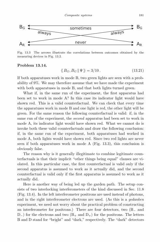
January 4, 2011 14:56 World Scientific Book - 9in x 6in main
Composite systems 181
Fig. 13.3 The arrows illustrate the correlations between outcomes obtained by themeasuring devices in Fig. 13.2.
Problem 13.14.
〈〈BG, BG ||Ψ 〉〉 = 3/10 . (13.21)
If both apparatuses work in mode B, two green lights are seen with a prob-
ability of 9%. We may therefore assume that we have made the experiment
with both apparatuses in mode B, and that both lights turned green.
What if, in the same run of the experiment, the first apparatus had
been set to work in mode A? In this case its indicator light would have
shown red. This is a valid counterfactual. We can check that every time
the apparatuses work in mode B and one light is red, the other light will be
green. For the same reason the following counterfactual is valid: if, in the
same run of the experiment, the second apparatus had been set to work in
mode A, its indicator light would have shown red. What we cannot do is
invoke both these valid counterfactuals and draw the following conclusion:
if, in the same run of the experiment, both apparatuses had worked in
mode A, both lights would have shown red. Since two red lights are never
seen if both apparatuses work in mode A (Fig. 13.3), this conclusion is
obviously false.
The reason why is it generally illegitimate to combine legitimate coun-
terfactuals is that their implicit “other things being equal” clauses are vi-
olated. In this particular case, the first counterfactual is valid only if the
second apparatus is assumed to work as it actually did, and the second
counterfactual is valid only if the first apparatus is assumed to work as it
actually did.
Here is another way of being led up the garden path. The setup con-
sists of two interlocking interferometers of the kind discussed in Sec. 11.8
(Fig. 13.4). In the left interferometer positrons are used instead of photons,
and in the right interferometer electrons are used. (As this is a gedanken
experiment, we need not worry about the practical problem of constructing
an interferometer for positrons.) There are four detectors, two (B− and
D−) for the electrons and two (B+ and D+) for the positrons. The letters
B and D stand for “bright” and “dark,” respectively. The “dark” detectors
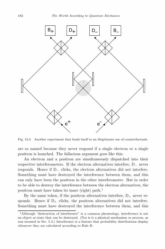
November 24, 2010 10:17 World Scientific Book - 9in x 6in main
182 The World According to Quantum Mechanics
Fig. 13.4 Another experiment that lends itself to an illegitimate use of counterfactuals.
are so named because they never respond if a single electron or a single
positron is launched. The fallacious argument goes like this:
An electron and a positron are simultaneously dispatched into their
respective interferometers. If the electron alternatives interfere, D− never
responds. Hence if D− clicks, the electron alternatives did not interfere.
Something must have destroyed the interference between them, and this
can only have been the positron in the other interferometer. But in order
to be able to destroy the interference between the electron alternatives, the
positron must have taken its inner (right) path.1
By the same token, if the positron alternatives interfere, D+ never re-
sponds. Hence if D+ clicks, the positron alternatives did not interfere.
Something must have destroyed the interference between them, and this
1Although “destruction of interference” is a common phraseology, interference is notan object or state that can be destroyed. (Nor is it a physical mechanism or process, aswas stressed in Sec. 5.3.) Interference is a feature that probability distributions displaywhenever they are calculated according to Rule B.
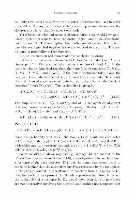
December 23, 2010 10:25 World Scientific Book - 9in x 6in main
Composite systems 183
can only have been the electron in the other interferometer. But in order
to be able to destroy the interference between the positron alternatives, the
electron must have taken its inner (left) path.
Yet if both particles had taken their inner paths, they would have anni-
hilated each other somewhere in the dotted region, and no detector would
have responded. The assumption that both dark detectors click if both
particles are dispatched together is thereby reduced to absurdity. The cor-
responding probability is therefore zero.
A quick calculation will show that this conclusion is wrong.
Let us call the electron alternatives O− (for “outer path”) and I− (for
“inner path”). The positron alternatives then are O+ and I+. If the
two particles are launched together, there are four alternatives: O− &O+,
O− & I+, I− &O+, and I− & I+. If the fourth alternative takes place, the
two particles annihilate each other, and no detector responds. Hence only
the first three alternatives contribute to the probability of “double dark
detection” (both D’s click). This probability is given by
p(D−&D+) = |a(O−&O+) + a(O−&I+) + a(I−&O+)|2
= |a(O−) a(O+) + a(O−) a(I+) + a(I−) a(O+)|2 . (13.22)
The amplitudes a(O−), a(I−), a(O+), and a(I+) are again equal except
that each contains an extra factor i for every reflection: a(O−) = Ai,
a(O+) = Ai, a(I−) = Ai3, and a(I+) = Ai3. Thus,
p(D−&D+) = |(Ai)(Ai) + (Ai)(Ai3) + (Ai3)(Ai)|2 = |A2|2 . (13.23)
Problem 13.15.
p(D−&B+) = p(B−&D+) = p(D−&D+) , p(B−&B+) = 9 p(D−&D+) .
Since the probability with which the two particles annihilate each other
is 1/4, the probability p(D−&D+)+p(D−&B+)+p(B−&D+)+p(B−&B+),
with which any two detectors respond, is (1 + 1 + 1 + 9)|A2|2 = 3/4. This
tells us that p(D−&D+) = |A2|2 = 1/16.
So where did the above argument go wrong? In the context of the
Elitzur–Vaidman experiment (Sec. 11.8), it was legitimate to conclude from
a response of the dark detector (D2) that the bomb was present, and to
conclude further that the alternative involving reflection by M2 took place.
In the present context, it is legitimate to conclude from a response of D+
that the electron was present, for if only a positron had been launched,
the probability of a response by D+ would have been 0. But now there
are two alternatives involving the positron, and nothing has happened that

November 24, 2010 10:17 World Scientific Book - 9in x 6in main
184 The World According to Quantum Mechanics
Fig. 13.5 The experiment of Englert, Scully, and Walther.
warrants the further conclusion that the electron has taken its inner path.
By the same token, nothing has happened that warrants the conclusion
that the positron has taken its inner path. What has once again led to the
wrong conclusion is our deep-seated misconception that effects have to be
locally produced.
13.7 The experiment of Englert, Scully, and Walther
Rule A (Sec. 5.1), you will recall, applies “if the intermediate measurements
are made (or if it is possible to find out what their outcomes would have
been if they had been made),” and Rule B applies “if the intermediate
measurements are not made (and if it is impossible to find out what their
outcomes would have been if they had been made).” The following two-slit
experiment [Englert et al. (1994); Scully et al. (1991)] demonstrates the
rationale behind the cryptic clauses in parentheses.
In this experiment atoms are used instead of electrons. All atoms are
of the same type—Cesium-133, for example—and all start out in the same
excited state |e〉. Placed in front of the slits are two initially separate

December 23, 2010 10:25 World Scientific Book - 9in x 6in main
Composite systems 185
microwave resonance cavities, each tuned to the energy difference ∆E be-
tween |e〉 and the ground state |g〉, and thus capable of holding photons2 of
energy ∆E. The design of each cavity moreover ensures that the probability
with which an atom is found to emerge from it in the ground state equals
unity—provided, as always, that the appropriate measurement is made.
13.7.1 The experiment with shutters closed
The two resonance cavities are separated from each other by a pair of
electro-optical shutters, which remain closed for now. Atoms are launched,
one at a time, with nothing to predict the particular cavity through which
any given atom will pass. (Before an atom is launched, the photon left
behind by the previous atom is “removed”: the possibility of detecting it
no longer exists.) Each atom leaves a mark on the screen. How will the
marks be distributed?
Focus on a single atom, after it has hit the screen but before the photon
is removed. This is a situation in which it is possible to find out what
the outcome of an intermediate measurement would have been if it had
been made. The intermediate measurement, had it been made, would have
determined the slit taken by the atom. The reason why we can find out what
its outcome would have been is a strict correlation between its outcome and
the cavity containing the photon. If the atom were found to emerge from
the left slit, the probability of detecting (and absorbing) a photon in the left
cavity would be 1, and if the atom were found to emerge from the right slit,
the probability of detecting (and absorbing) a photon in the right cavity
would be 1. Conversely, if a photon is detected in the left (right) cavity, a
measurement of the slit taken by the atom would have indicated that the
atom has taken the left (right) slit.
Thus Rule A applies. Let us color the marks: those made by atoms that
left a photon in the left cavity green, and those made by atoms that left
a photon in the right cavity red. The dotted curve in Fig. 13.6 gives the
distribution of the green marks, the dashed curve that of the red marks.
The solid curve is the sum of the two distributions. The green marks are
distributed as we expect from atoms that went through the left slit (L), and
the red marks are distributed as we expect from atoms that went through
the right slit (R). (Compare Fig. 13.6 with Fig. 5.2.)
2In what sense can a cavity hold a photon? In precisely this conditional sense: if a(100% efficient) photodetector were inserted into the cavity, it would detect a photonwith probability 1.
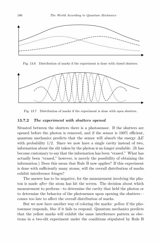
November 24, 2010 10:17 World Scientific Book - 9in x 6in main
186 The World According to Quantum Mechanics
Fig. 13.6 Distribution of marks if the experiment is done with closed shutters.
Fig. 13.7 Distribution of marks if the experiment is done with open shutters.
13.7.2 The experiment with shutters opened
Situated between the shutters there is a photosensor. If the shutters are
opened before the photon is removed, and if the sensor is 100% efficient,
quantum mechanics predicts that the sensor will absorb the energy ∆E
with probability 1/2. Since we now have a single cavity instead of two,
information about the slit taken by the photon is no longer available. (It has
become customary to say that the information has been “erased.” What has
actually been “erased,” however, is merely the possibility of obtaining the
information.) Does this mean that Rule B now applies? If this experiment
is done with sufficiently many atoms, will the overall distribution of marks
exhibit interference fringes?
The answer has to be negative, for the measurement involving the pho-
ton is made after the atom has hit the screen. The decision about which
measurement to perform—to determine the cavity that held the photon or
to determine the behavior of the photosensor upon opening the shutters—
comes too late to affect the overall distribution of marks.
But we now have another way of coloring the marks: yellow if the pho-
tosensor responds, blue if it fails to respond. Quantum mechanics predicts
that the yellow marks will exhibit the same interference pattern as elec-
trons in a two-slit experiment under the conditions stipulated by Rule B

November 24, 2010 10:17 World Scientific Book - 9in x 6in main
Composite systems 187
(Fig. 5.3). Because the overall distribution of marks is the same in both
versions of the experiment, the blue marks will exhibit the complementary
interference pattern, having maxima where the other has minima and vice
versa. The dotted curve in Fig. 13.7 gives the distribution of yellow marks,
the dashed curve that of blue marks. The solid curve—the sum of the two
distributions—is the same as in Fig. 13.6.
All “yellow” atoms and all “blue” atoms have something in common,
but as their respective behaviors lack classical counterparts, we have no
ready name for it. We may say that the “yellow” atoms went through the
slits in phase, while the “blue” atoms went through the slits out of phase.
We use these phrases for the following reason. If there is to be a maxi-
mum at the center of the screen, the phases of the amplitudes associated
with the alternatives “through L” and “through R” must differ by an even
multiple of π—the alternatives must be “in phase.” And if there is to be a
minimum instead, the amplitudes must differ by an odd multiple of π—the
alternatives must be “out of phase.”
13.7.3 Influencing the past
The “green” atoms, we noted, behave like atoms that went through L,
while the “red” atoms behave like atoms that went through R. Likewise,
the “yellow” atoms behave like atoms that went through the slits in phase
(inasmuch as they display the corresponding interference pattern), while
the “blue” atoms behave like atoms that went through the slits out of
phase. Cannot we conclude from this that the “green” atoms actually went
through L, that the “red” atoms actually went through R, that the “yellow”
atoms actually went through the slits in phase, and that the “blue” atoms
actually went through the slits out of phase? After all, if it looks like a
duck, swims like a duck, and quacks like a duck, then it probably is a duck.
The problem with this conclusion is that it seems to imply the possibility
of influencing the past.
If the experimenters determine the cavity that held the photon, they
learn through which slit the corresponding atom went. If they open the
shutters and observe whether or not the sensor responds, they learn how the
atom went through the slits—in phase or out of phase. They cannot make
the atom go through L or through R, yet by doing the former experiment,
they can make sure that it went through a single slit—either L or R. Nor
can they make an atom go through the slits in phase or out of phase, yet by
doing the latter experiment they can make sure that it when through both

November 24, 2010 10:17 World Scientific Book - 9in x 6in main
188 The World According to Quantum Mechanics
Fig. 13.8 Logical flow chart for the experiment of Englert, Scully, and Walther.
slits.3 And since they can choose between the two experiments after the
atom has made its mark on the screen, they can, by their choice, contribute
to determine the atom’s past behavior (Fig. 13.8).
Before rejecting the assumptions that lead to this conclusion, we need
to be clear about what they amount to. Saying that a “green” atom went
through L cannot mean that this very atom would also have gone through L
if the cavity containing the photon emitted by it had not been ascertained.
For if this cavity had not been ascertained, the experimenters could have
checked how the atom went through both slits (in phase or out of phase),
3For more on the meaning of “both” see Sec. 18.1.2.

December 23, 2010 10:25 World Scientific Book - 9in x 6in main
Composite systems 189
and regardless of the outcome they would have found that it went through
both slits.
Rather, a “green” atom went through L only because this is what was
indicated by a measurement. An atom goes through a particular slit only
if the appropriate measurement is made, and it goes through L only if this
is the outcome. It goes through both slits with a particular phase relation
only if a different measurement is made, and it goes through both slits in
phase only if that is the outcome. If neither measurement is made, it does
not go through the left slit and it does not go through the right slit and it
does not go through both slits in phase and it does not go through both slits
out of phase. To paraphrase a well-known conclusion by John Wheeler,4 no
property (or behavior) is a possessed (occurrent) property (behavior) unless
it is a measured (or indicated) property (behavior). Quantum-mechanical
measurements do not merely reveal pre-existent properties or behaviors
that occurred independently of measurements; they create their outcomes.
Seen in this light, the possibility of partially determining an atom’s past
behavior no longer seems preposterous. If, as a general rule, the properties
of the quantum world exist only if, and only to the extent that, they are
measured,5 then the behavior of a quantum system at an earlier time can
depend on a measurement performed at a later time, and thus also on a
decision taken at a later time. Nothing like the backward-in-time causation
found in some fantasy novels, which changes the past, is suggested. By
choosing to perform either experiment, the experimenters cause no change
in the atom’s past behavior. Rather, they contribute to create or determine
its past behavior. The world has exactly one history. Its state at any given
time is what it is; it cannot be changed. But it can be what it is because
of a measurement performed at a later time.6
But still, if no behavior is an occurrent behavior unless it is a measured
or indicated behavior, we have reasons to doubt that the “green” atoms
actually went through L. Strictly speaking, the conclusion that is warranted
by the detection of a photon in the left cavity is this: the corresponding
atom would have been found taking the left slit if a direct measurement of
the slit taken by the atom had been made. But here we need to take into
account that no measurement is direct. Measurement outcomes are inferred
4“No elementary phenomenon is a phenomenon until it is a registered (observed) phe-nomenon” [Wheeler (1983)].5This issue will be conclusively addressed in Sec. 16.3.6In fact, property-indicating events occur quite generally after the time of possession
of the indicated property, albeit usually a fairly short time after.
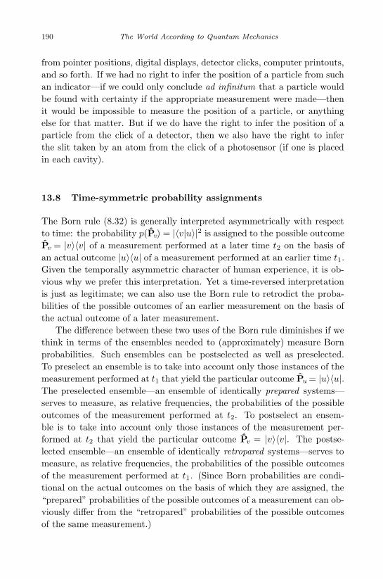
November 24, 2010 10:17 World Scientific Book - 9in x 6in main
190 The World According to Quantum Mechanics
from pointer positions, digital displays, detector clicks, computer printouts,
and so forth. If we had no right to infer the position of a particle from such
an indicator—if we could only conclude ad infinitum that a particle would
be found with certainty if the appropriate measurement were made—then
it would be impossible to measure the position of a particle, or anything
else for that matter. But if we do have the right to infer the position of a
particle from the click of a detector, then we also have the right to infer
the slit taken by an atom from the click of a photosensor (if one is placed
in each cavity).
13.8 Time-symmetric probability assignments
The Born rule (8.32) is generally interpreted asymmetrically with respect
to time: the probability p(Pv) = |〈v|u〉|2 is assigned to the possible outcome
Pv = |v〉〈v| of a measurement performed at a later time t2 on the basis of
an actual outcome |u〉〈u| of a measurement performed at an earlier time t1.
Given the temporally asymmetric character of human experience, it is ob-
vious why we prefer this interpretation. Yet a time-reversed interpretation
is just as legitimate; we can also use the Born rule to retrodict the proba-
bilities of the possible outcomes of an earlier measurement on the basis of
the actual outcome of a later measurement.
The difference between these two uses of the Born rule diminishes if we
think in terms of the ensembles needed to (approximately) measure Born
probabilities. Such ensembles can be postselected as well as preselected.
To preselect an ensemble is to take into account only those instances of the
measurement performed at t1 that yield the particular outcome Pu = |u〉〈u|.The preselected ensemble—an ensemble of identically prepared systems—
serves to measure, as relative frequencies, the probabilities of the possible
outcomes of the measurement performed at t2. To postselect an ensem-
ble is to take into account only those instances of the measurement per-
formed at t2 that yield the particular outcome Pv = |v〉〈v|. The postse-
lected ensemble—an ensemble of identically retropared systems—serves to
measure, as relative frequencies, the probabilities of the possible outcomes
of the measurement performed at t1. (Since Born probabilities are condi-
tional on the actual outcomes on the basis of which they are assigned, the
“prepared” probabilities of the possible outcomes of a measurement can ob-
viously differ from the “retropared” probabilities of the possible outcomes
of the same measurement.)

November 24, 2010 10:17 World Scientific Book - 9in x 6in main
Composite systems 191
Quantum mechanics even allows us to assign probabilities symmetrically
with respect to time, on the basis of both earlier and later outcomes.
Suppose that three measurements are performed at the respective times
t1 < t2 < t3, that the measurement at t1 yields the outcome u (represented
by the projector |u〉〈u|), and that the measurement at t3 yields the outcome
w (represented by the projector |w〉〈w|). We can calculate the probability
p(v|w, u) with which the outcome v (represented by the projector |v〉〈v|) is
obtained at t2 taking both data into account.
To measure this probability as a relative frequency, we use an ensem-
ble that is both pre- and postselected (i.e., an ensemble of systems that
are identically retropared as well as identically prepared). To create the
appropriate ensemble, we take into account (i) only those instances of the
measurement performed at t1 that yield u and (ii) only those instances of
the measurement performed at t3 that yield w. In other words, we discard
all runs in which the first measurement yields an outcome different from u
and the third measurement yields an outcome different from w.
To calculate p(v|w, u), we start from Eq. (1.8) but include in each term
a condition c:
p(b|a,c) =p(a,b|c)p(a|c) . (13.24)
In the present context this reads
p(v|w,u) =p(w,v|u)pV(w|u) . (13.25)
p(w,v|u) is the probability of obtaining both v and w by the respective
measurements at t2 and t3, on the condition that u is obtained at t1. It
is given by the product p(w|v) p(v|u) of two Born probabilities. pV(w|u)is the probability of obtaining w at t3 given that u is obtained at t1 and
given that the measurement with the possible outcome v is made at t2.
The subscript V stands for the observable that is measured at t2. Since we
calculate the probability with which this measurement yields v, we must
use pV(w|u) rather than the Born probability p(w|u) = |〈w|u〉|2, which is
applicable only if no measurement is made between t1 and t3. As the inter-
mediate measurement is assumed to be made, Rule A applies, so pV(w|u)is given by
pV(w|u) =
n∑
i=1
p(w, vi|u) , (13.26)

November 24, 2010 10:17 World Scientific Book - 9in x 6in main
192 The World According to Quantum Mechanics
where the values vi, i = 1, 2, . . . , n, are the possible outcomes of a mea-
surement of V . Setting v = vk, we arrive at the ABL rule [Aharonov,
Bergmann, and Lebowitz (1964)]:
p(vk|w, u) =|〈w|vk〉〈vk |u〉|2
∑ni=1 |〈w|vi〉〈vi|u〉|2
. (13.27)
13.8.1 A three-hole experiment
It will be instructive to apply the ABL rule to the following setup. This
features a plate with three holes in it; let us call them A, B, and C. In
front of the plate and equidistant from the holes there is a particle source
(say, an electron gun G), and behind the plate, again equidistant from the
holes, there is a particle detector D. Finally, interposed between C and D
there is a device that causes a phase shift by π. An electron emerging from
the holes is thus prepared in a way that can be “described” by the vector
|1〉 = 1√3
(|A〉+ |B〉+ |C〉
), (13.28)
and it is retropared in a way that can be “described” by the vector
|2〉 = 1√3
(|A〉+ |B〉 − |C〉
). (13.29)
The factor eiπ = −1 in front of |C〉 takes account of the phase shifting
device.
We now add an apparatus MA that can indicate whether or not a par-
ticle went through A. The two possible outcomes of this measurement are
represented by PA = |A〉〈A| (“through A”) and PA′ = PB + PC (“not
through A”). The probability that a particle launched at G and detected
at D is found to have gone through A is thus
p(A|2, 1) =|〈2|PA|1〉|2
|〈2|PA|1〉|2 + |〈2|PA′ |1〉|2. (13.30)
Problem 13.16. |〈2|PA′ |1〉|2 = 0.
Thus p(A|2, 1) = 1. With this setup, a particle launched at G and detected
at D is certain to be found taking hole A.
If, instead of MA, we use an apparatus MB that can indicate whether or
not a particle went through B, we similarly find that p(B|2, 1) = 1. With
this setup, a particle launched at G and detected at D is certain to be found
taking hole B.

November 24, 2010 10:17 World Scientific Book - 9in x 6in main
Composite systems 193
Finally we use an apparatus that can indicate through which of the three
holes a particle went. The three possible outcomes of this measurement are
represented by PA, PB , and PC . The probability that a particle launched
at G and detected at D is found taking hole A now equals
p(A|2, 1) =|〈2|PA|1〉|2
|〈2|PA|1〉|2 + |〈2|PB |1〉|2 + |〈2|PC |1〉|2=
1
3. (13.31)
Time-symmetric probability assignments thus are in general contextual.
The probability with which a particle launched at G and detected at D
is found to go through A depends on the possible outcomes of the interme-
diate measurement. If the only possible outcome other than A is A′, then
p(A|2, 1) = 1, and if the possible outcomes other than A are B and C, then
p(A|2, 1) = 1/3.7
7Although the present section does not fall under the heading of the present chapter, itsinclusion is warranted by the contextuality that time-symmetric probability assignmentsshare with probability assignments to outcomes of measurements performed on entangledsystems.

November 24, 2010 10:17 World Scientific Book - 9in x 6in main
This page intentionally left blankThis page intentionally left blank

November 24, 2010 10:17 World Scientific Book - 9in x 6in main
Chapter 14
Quantum statistics
14.1 Scattering billiard balls
Two billiard balls coast toward each other with equal speed, then collide.
Initially the balls move in opposite directions, so their momenta add up
to zero. Because momentum is conserved, the total momentum remains
zero, so after the collision the balls still move with equal speed in opposite
directions. If the collision is perfectly head-on, each ball simply reverses
its direction of motion. But suppose that the collision is uncontrollably
somewhat off-center, so that each ball veers from its original direction of
motion by some angle α. We cannot predict whether the balls will scatter
at right angles (plus/minus some small angle ε), but we can estimate the
probability with which they will do so.
There are two ways in which the balls can scatter at right angles. If we
call the incoming balls N and S (suggesting that they move northward and
southward, respectively), we may call the outgoing balls E and W . If either
ball is as likely to be scattered eastward as westward, the corresponding
probabilities are equal:
p(N→W,S→E) = p(N→E, S→W )Def= p . (14.1)
The probability p⊥ with which either possibility happens, no matter which,
is the sum of these two probabilities:
p⊥ = p(N→W,S→E) + p(N→E, S→W ) = 2p . (14.2)
14.2 Scattering particles
We now replace the billiard balls with particles (Fig. 14.1). We again
assume that the total momentum is zero, and that the scattering is elastic;
195

November 24, 2010 10:17 World Scientific Book - 9in x 6in main
196 The World According to Quantum Mechanics
Fig. 14.1 The two possibilities that contribute to the probability with which two par-ticles scatter elastically at right angles. The lines do not represent trajectories; theymerely indicate possible identities between the incoming and outgoing particles.
in a particle context this means that no particles are created or annihilated
in the process and that no type swapping takes place. If the incoming
particles (and hence the outgoing ones) are of different types, then it is
possible to learn which outgoing particle is identical with which incoming
particle, so Rule A applies:
p⊥ = |A(N→W,S→E)|2 + |A(N→E, S→W )|2. (14.3)
This is again the sum of two probabilities. If there are no preferred direc-
tions (due to external forces, particle spins, and such), the two probabilities
are equal,
|A(N→W,S→E)|2 = |A(N→E, S→W )|2 Def= p , (14.4)
and we again have that p⊥ = 2p.
But now suppose that the conditions stipulated by Rule B are met. This
rules out, among other things, that the incoming particles are of different
types. We then have that
p⊥ = |A(N→W,S→E) +A(N→E, S→W )|2. (14.5)
Equation (14.4) allows the amplitudes to differ by a phase factor:
ADef= A(N→W,S→E) = eiφA(N→E, S→W ) . (14.6)
Interchanging either the incoming or the outgoing particles, so that the
alternative N→E, S→W turns into the alternative N→W,S→E, causes
the multiplication of A(N→E, S→W ) by eiφ. Accordingly, interchanging

December 23, 2010 10:25 World Scientific Book - 9in x 6in main
Quantum statistics 197
either the incoming or the outgoing particles twice, or interchange both the
incoming particles and the outgoing particles, corresponds to a multiplica-
tion of A(N→E, S→W ) by (eiφ)2. But this simply restores the original
alternative. It follows that (eiφ)2 = 1, and this leaves eiφ = ±1 as the only
possibilities.
Nature makes use of both possibilities. Every particle is either a boson or
a fermion. Exchanging two indistinguishable bosons leaves the amplitudes
unchanged,
A(N→W,S→E) = A(N→E, S→W ) , (14.7)
whereas exchanging two indistinguishable fermions causes a change of sign,
A(N→W,S→E) = −A(N→E, S→W ) . (14.8)
For bosons, therefore,
p⊥ = |A+A|2 = 4|A|2 = 4p , (14.9)
whereas for fermions
p⊥ = |A−A|2 = 0 . (14.10)
Two indistinguishable bosons are twice as likely to scatter at right angles
as two bosons that carry identity tags of some sort, while the probability
with which two indistinguishable fermions scatter at right angles equals
zero.
Can we nevertheless assume that there is an answer to the question
“Which outgoing particle is identical with which incoming particle?” We
cannot, for it this question had an answer, what actually happened would
correspond to either of the alternatives of Fig. 14.1, and in this case we
would have p⊥ = 2p instead of either p⊥ = 4p or p⊥ = 0.
14.2.1 Indistinguishable macroscopic objects?
Could the identities of macroscopic objects, such as billiard balls, get
“mixed up” in this way?
For one thing, macroscopic objects are so large and/or complex that the
likelihood with which two such objects are truly indistinguishable is virtu-
ally zero. For another, while it is relatively easy to adequately isolate two
particles from the rest of the world, isolating sufficiently large or complex
objects is virtually impossible. Even if the cosmic microwave background
radiation were the only source of photons, such objects would continually
absorb and emit photons with wavelengths in the millimeter range, and this

November 24, 2010 10:17 World Scientific Book - 9in x 6in main
198 The World According to Quantum Mechanics
would make it possible to pinpoint each object’s location to within a few
millimeters or less. If the objects are larger than that, then it is possible to
trace their respective trajectories with sufficient precision to know which is
which.
14.3 Symmetrization
Suppose that we have two bosons, and that their respective states are |A〉and |B〉. And suppose that these bosons are fully characterized by their
respective states. If we write the state of the composite system as |A〉 ⊗ |B〉,or simply |AB〉, we add to the physically warranted distinction between
“the boson associated with |A〉” and “the boson associated with |B〉” the
physically unwarranted distinction between the “first” or “left” boson and
the “second” or “right” boson.
If |A〉 and |B〉 are orthogonal states, we can eliminate the physically
unwarranted distinction by associating the composite system with the sym-
metric state
|AB〉+ |BA〉√2
, (14.11)
which is invariant under the interchange of A and B.
Problem 14.1. If each of the orthogonal vectors |A〉 and |B〉 is a unit
vector, then so is (14.11).
Let |A〉, |B〉, |C〉, . . . be mutually orthogonal boson states. Properly sym-
metrized multiple-boson states are obtained by adding all distinct permu-
tations and dividing by the square root of their number. The symmetrized
three-boson states are thus of the form
|AAA〉, 1√3
(
|AAB〉 + |ABA〉+ |BAA〉)
,
1√6
(
|ABC〉 + |ACB〉+ |BAC〉 + |BCA〉+ |CAB〉 + |CBA〉)
.
14.4 Bosons are gregarious
If n bosons have been found in possession of the same complete set of
properties X and one boson has been found in possession of a different
complete set of properties Y , what is the probability of finding all n + 1

January 4, 2011 14:56 World Scientific Book - 9in x 6in main
Quantum statistics 199
bosons in possession of X? (A complete set of properties is what a complete
measurement yields.) The initial and final states are, respectively,
|i〉 = 1√n+ 1
(
|n
︷ ︸︸ ︷
X . . .X Y 〉+ · · ·+ |n−m︷ ︸︸ ︷
X . . .X Y
m︷ ︸︸ ︷
X . . .X〉+ · · ·+ |Yn
︷ ︸︸ ︷
X . . .X〉)
|f〉 = |n+1
︷ ︸︸ ︷
X . . .X〉The transition amplitude thus is
1√n+ 1
(
〈n+1
︷ ︸︸ ︷
X . . .X |n
︷ ︸︸ ︷
X . . .X Y 〉+ · · ·+ 〈n+1
︷ ︸︸ ︷
X . . .X |Yn
︷ ︸︸ ︷
X . . .X〉)
. (14.12)
Since the n+1 terms in brackets are equal to 〈X |X〉n〈X |Y 〉, this amplitude
is equal to
n+ 1√n+ 1
〈n+1
︷ ︸︸ ︷
X . . .X |n
︷ ︸︸ ︷
X . . .X Y 〉 =√n+ 1 〈
n+1︷ ︸︸ ︷
X . . .X |n
︷ ︸︸ ︷
X . . .X Y 〉 . (14.13)
The wanted probability thus is (n+ 1) |〈n+1
︷ ︸︸ ︷
X . . .X |n
︷ ︸︸ ︷
X . . .X Y 〉|2.If we were dealing with distinguishable (“tagged”) bosons (in which case
X and Y would not be complete sets of properties), the initial state would
be the non-symmetrized vector
|n
︷ ︸︸ ︷
X . . .X Y 〉 ,
and the transition probability would be |〈n+1
︷ ︸︸ ︷
X . . .X |n
︷ ︸︸ ︷
X . . .X Y 〉|2.The upshot: if n bosons of a given type have been found in possession
of the same complete set of properties X and one boson of the same type
has been found in possession of a different complete set of properties Y , the
probability of finding all n+ 1 bosons in possession of X is n+ 1 times as
large as it would be if the bosons were distinguishable.
14.5 Fermions are solitary
Fermion amplitudes change sign each time states are swapped between par-
ticles. Fermion states must therefore be anti-symmetrized. Since no anti-
symmetric state can be formed of two identical fermion states, the prob-
ability of finding two fermions in possession of the same complete set of
properties is zero. This is the content of the exclusion principle originally
formulated by Wolfgang Pauli.

January 4, 2011 14:56 World Scientific Book - 9in x 6in main
200 The World According to Quantum Mechanics
14.6 Quantum coins and quantum dice
We refer to the statistics of identical bosons as Bose–Einstein (BE) statis-
tics, to that of identical fermions as Fermi–Dirac (FD) statistics, and to
that of distinguishable particles as Maxwell–Boltzmann (MB) statistics.
As we all know, the probability with which a toss of a pair of MB coins
results in two heads, pMB(HH), equals p(H) × p(H) = 1/4. Since MB
coins are distinguishable, there are two ways in which one comes up heads
and one comes up tails, so the odds for this to happen are given by the sum
of two probabilities, pMB(HT ) + pMB(TH) = 1/2.
For a pair of FD coins, there is a single possible outcome, one heads
and one tails, so the odds for this to happen equals unity. What about
BE coins? The probability of tossing the first H is p(H) = 1/2. The
probability of subsequently tossing another H is twice the probability of
subsequently tossing a T, p(H |H) = 2p(T |H), for the factor n + 1 equals
2 in this case. Because we must have that p(T |H) + p(H |H) = 1, we
conclude that p(T |H) = 1/3 and p(H |H) = 2/3. The joint probability
p(HH)—not to be confused with the conditional probability p(H |H)—
equals p(H |H) p(H) = (2/3) (1/2) = 1/3. Similarly we find that p(TT ) =
1/3. And since there is now only one way of obtaining one H and one T ,
the probability for this to happen is 1 − (1/3) − (1/3) = 1/3. Note that
the possible outcomes are again equiprobable. Only in the case of MB
coins there are four possibilities while in the case of BE coins there are
three.
Problem 14.2. (∗) When tossing a pair of MB dice, the probability of
obtaining the sum of 12, pMB(12), equals 1/6 × 1/6 = 1/36. There are
two ways of obtaining the sum of 11, so pMB(11) is twice that. By the
same token, pMB(10) = 3/36, pMB(9) = 4/36, and so on. What are the
corresponding probabilities when tossing (i) a pair of BE dice and (ii) a
pair of FD dice?
The outcomes of tosses of MB dice are uncorrelated. The probabilities
assigned to the possible outcomes of one toss are independent of the out-
come of another toss. In particular, the probability of obtaining a 6 is 1/6
regardless of how many dice already have come up 6. The outcomes of
tossing BE dice or FD dice, on the other hand, are correlated. For BE dice,
the probability of obtaining a 6 increases with the number of dice already
showing a 6, while for FD dice the probability of obtaining a 6 is zero unless
no other die is showing a 6.

November 24, 2010 10:17 World Scientific Book - 9in x 6in main
Quantum statistics 201
What mechanism or process could possibly explain the correlations that
obtain between indistinguishable particles? Misner et al. (1973) have an-
swered this question succinctly: “No acceptable explanation for the mirac-
ulous identity of particles of the same type has ever been put forward. That
identity must be regarded, not as a triviality, but as a central mystery of
physics.”
14.7 Measuring Sirius
The telescopic image of a pointlike light source is a disk whose diameter
depends inversely on the telescope’s aperture. For the largest telescopes,
the angles subtended by the nearest or largest fixed stars are of the order of
the diameter of this disk. At least this was true in 1956, when R. Hanbury
Brown and R.Q. Twiss (1956) (HBT) showed how the angular diameter
of a fixed star could be measured. HBT proposed to use two telescopes
pointed at the same star. By fitting the telescopes with photomultipliers,
they argued, the star’s angular diameter could be deduced from correlations
between variations of the photon detection rates through the telescopes.
The arguments of HBT were greeted with considerable disbelief, and
various theoretical and experimental efforts were made to disprove them.
Photons, it was thought, are emitted one at a time and detected one at a
time. A photon is detected by either of the photomultipliers—M1 or M2.
No photon is detected by both M1 and M2. So how could the photon counts
be correlated? It was even thought that if HBT were correct, quantum
mechanics was in need of thorough revision.
In 1965, an intensity interferometer using two paraboloid mirrors with
a diameter of 6.5m and a variable baseline (from 10 to 188 meters) was
completed in Australia, and by the end of the decade, HBT had measured
the angular diameters of more than twenty stars with remarkable accuracy,
confounding those who had argued that their interferometer could not work
[Hanbury Brown et al. (1967); Hanbury Brown (1968)].
The best way of demonstrating the error of HBT’s critics is to go ahead
and calculate. We first assume that there are two light sources. Let a(y|x)be the amplitude associated with what we are used to calling “the emission
of a photon” at x = A or x = B (the positions of the light sources) and
“its absorption” at y = 1 or y = 2 (the positions of the telescopes). Let
ryx stand for the distance between x and y. The absolute value of a(y|x)is inverse proportional to ryx. Let the corresponding proportionality factor

November 24, 2010 10:17 World Scientific Book - 9in x 6in main
202 The World According to Quantum Mechanics
Fig. 14.2 Above: two indistinguishable alternatives; below: two distinguishable alter-natives.
be α for the source at A and β for the source at B. The phase of a(y|x) is
proportional to ryx. We may assume that the corresponding proportionality
factor is the same wavenumber k = 2π/λ for both sources. (Each telescope
is fitted with a narrow bandpass filter, so that λ has a well-defined value.)
Because the differences between the absolute values of the four amplitudes
are minute as compared to the absolute values themselves, we may use
a(1|A) =α
Reikr1A , a(1|B) =
β
Reikr1B ,
a(2|A) =α
Reikr2A , a(2|B) =
β
Reikr2B .
R is defined by Fig. 14.3.
The simultaneous detection at 1 and 2 of photons emitted at A or B can
come about in four ways. Two of the four alternatives—those with photons
emitted by different sources as indicated in the upper half of Fig. 14.2—are
indistinguishable, and two—those with photons emitted by the same source
as indicated in the lower half of Fig. 14.2—are distinguishable, both from
each other and from the indistinguishable alternatives. (By measurements
performed on the sources at A and at B, it is in principle possible to learn
how many photons were emitted by each source.) The amplitudes of the
indistinguishable alternatives are

November 24, 2010 10:17 World Scientific Book - 9in x 6in main
Quantum statistics 203
Fig. 14.3 Schematic of the parameters used in Hanbury Brown and Twiss’s calculationof the angular diameter of a star.
a(1|A) a(2|B) =αβ
R2eik(r1A+r2B),
a(1|B) a(2|A) =αβ
R2eik(r1B+r2A).
Because the alternatives are indistinguishable, we must add their ampli-
tudes. The corresponding probability is therefore given by
pI =α2β2
R4
(
eik(r1A+r2B) + eik(r1B+r2A))(
e−ik(r1A+r2B) + e−ik(r1B+r2A))
=α2β2
R4
(
2 + eik(r1A+r2B−r1B−r2A) + eik(r1B+r2A−r1A−r2B))
=2α2β2
R4
(
1 + cos [k(r1A + r2B − r1B − r2A)])
. (14.14)
To this we have to add the probabilities of detecting photons from the same
source. The probability of simultaneously detecting two photons thus is
P = pI + |a(1|A) a(2|A)|2 + |a(1|B) a(2|B)|2 = pI +α4
R4+β4
R4
=1
R4
[
α4 + β4 + 2α2β2(
1 + cos [k(r1A + r2B − r1B − r2A)])]
.
The angles δ1 and δ2 in what follows are defined by Fig. 14.3. Because
R� D, where D is the distance between A and B, we have that
δ1 ≈r1B − r1A
D=r2A − r2B
D≈ δ2 ≈
d
2R,
December 23, 2010 10:25 World Scientific Book - 9in x 6in main
204 The World According to Quantum Mechanics
where d is the distance between the telescopes. For the argument
(2π/λ)(r1A + r2B − r1B − r2A) of the cosine we can therefore write
(2π/λ) dD/R. As the distance between the telescopes is changed, the value
of the cosine oscillates between +1 and −1. Let ∆ be the amount by which
d has to increase so that the argument of the cosine completes a cycle:
2π∆D
λR= 2π . (14.15)
The angle D/R between the sources thus equals λ/∆.
Finally we must take into account that we have a disk-shaped source
rather than two pointlike ones. Doing so involves integration over the radius
of the disk. The angular diameter of the star is then obtained in much the
same way from the variation of the resulting probability P with ∆.

November 24, 2010 10:17 World Scientific Book - 9in x 6in main
Chapter 15
Relativistic particles
15.1 The Klein–Gordon equation
Formally the complete Schrodinger equation (7.23) can be obtained by the
following steps. Start with the non-relativistic relation between kinetic
energy and kinetic momentum, EK = p2K/2m. Write this in terms of the
total energy E, the total momentum p, the potential energy EP = qV (r, t),
and the potential momentum pP = (q/c)A(r, t) (Sec. 9.3):
E − qV =1
2m
(
p− q
cA)2
. (15.1)
Multiply both sides from the right by ψ(r, t), and replace the total energy
and the total momentum by the respective operators E = i~ ∂/∂t and
p = −i~ ∂/∂r (Sec. 11.6):
(
i~∂
∂t− qV
)
ψ =1
2m
(~
i
∂
∂r− q
cA)2
ψ . (15.2)
When we obtained the non-relativistic expressions for EK and pK from the
relativistic expressions (9.19) and (9.20), we found that the kinetic parts of
the relativistic expressions satisfy the relation (9.21). Using units in which
c = 1, as is customary in the literature on relativistic quantum mechanics,
this relation is
E2 − p2 = m2.
If we start with this relation and follow the same steps, we arrive at the rel-
ativistic version of the Schrodinger equation, which is known as the Klein–
Gordon equation (although it was Schrodinger who considered it first):[(
i~∂
∂t− qV
)2
−(
~
i
∂
∂r− qA
)2]
ψ = m2ψ . (15.3)
205

November 24, 2010 10:17 World Scientific Book - 9in x 6in main
206 The World According to Quantum Mechanics
Fig. 15.1 Some of the paths over which we sum when calculating a non-relativistic
particle propagator.
15.2 Antiparticles
As we noted in Sec. 4.1, any function of the form ψ(r, t) = Ae(i/~)(−Et+p·r)
satisfying the relation E = p2/2m is a solution of the free Schrodinger
equation, and so is any linear combination of such functions. By the same
token, any function of the same form satisfying the relation E2−p2 = m2,
or E = ±√
m2 + p2, is a solution of the free Klein–Gordon equation, and
so is any linear combination of such functions. What, then, are we to make
of solutions that seem to have negative energy?
When we introduced the (non-relativistic) propagator in the form of
a path integral (Sec. 5.4), the summation extended over all paths leading
from an initial to a final spacetime point, provided that velocities remained
finite (Fig. 15.1). In the relativistic theory, spacelike path segments are
exponentially suppressed rather than explicitly excluded (Sec. 9.1). But if
paths with spacelike segments are not explicitly excluded, then paths that
make U–turns with respect to time are not excluded either. If the speed of
light can be exceeded, there is nothing to prevent a particle from returning
into the past.
Two such paths are shown in Fig. 15.2. Paths in the vicinity of the solid
curve, containing as they do sizable spacelike segments, make no significant
contribution to a particle’s amplitude of propagation from A to B. The
same cannot be said of paths in the vicinity of the dashed curve, inasmuch

November 24, 2010 10:17 World Scientific Book - 9in x 6in main
Relativistic particles 207
Fig. 15.2 Two paths that contribute to the particle propagator in a relativistic theory.
as this lacks spacelike segments. This path makes two U–turns (or rather,
V–turns) with respect to time. According to a point of view advocated
by Feynman (1949), a particle traveling in the positive time direction with
negative energy is a particle traveling in the negative time direction with
positive energy.1 In more conventional terms, it is an antiparticle, which has
the same mass and total spin as the corresponding particle but the opposite
charge. Feynman’s account of the dashed path in Fig. 15.2 is that a particle
starts out at A, is scattered into a negative time direction at t2, is scattered
back into a positive time direction at t1, and arrives at B. The conventional
chronology, on the other hand, is that (i) a particle is launched at tA, (ii) a
particle-antiparticle pair is created at t1, (iii) the particle launched at tAand the antiparticle created at t1 annihilate each other at t2, and (iv) the
particle created at t1 is detected at tB .
15.3 The Dirac equation
The utility of the Klein–Gordon equation is restricted to particles with-
out spin. To arrive at the appropriate equation for a particle with spin,
one needs to let the wave function have more than one component. This
equation will therefore be a matrix equation. The simplest version is
1This chimes in with our observation in Sec. 6.6 that for antiparticles the sign of propertime differs from that of coordinate time.

December 23, 2010 10:25 World Scientific Book - 9in x 6in main
208 The World According to Quantum Mechanics
linear in the operators of energy and momentum. If one requires in addition
that each component of ψ should satisfy the Klein-Gordon equation, one
finds that the lowest possible number of components is four, and that this
number yields the appropriate equation for a spin-1/2 fermion—the Dirac
equation:(
i~∂
∂t− qV
)
ψ −α ·(
~
i
∂
∂r− qA
)
ψ = βmψ . (15.4)
β and the three components (α1, α2, α3) of α are 4 × 4 matrices, and ψ is
an 4× 1 matrix called a spinor. A possible choice for these matrices is
α1 =
0 0 0 +1
0 0 +1 0
0 +1 0 0
+1 0 0 0
, α2 =
0 0 0 −i0 0 +i 0
0 −i 0 0
+i 0 0 0
,
α3 =
0 0 +1 0
0 0 0 −1+1 0 0 0
0 −1 0 0
, β =
+1 0 0 0
0 +1 0 0
0 0 −1 0
0 0 0 −1
.
Note that the 2 × 2 matrices that make up the upper right and lower left
quarters of the three α matrices are the Pauli spin matrices (12.26). The
components of ψ correspond to the 2 + 2 spin components of a spin-1/2
particle and its antiparticle. A more compact way of writing the Dirac
equation (15.4) is[
iγk(
∂
∂xk+ iqAk
)
−m]
ψ = 0 , (15.5)
where γ0Def= β and γa
Def= βαa (a = 1, 2, 3). In the non-relativistic limit the
Dirac equation reduces to the Pauli equation,(
i~∂
∂t− qV
)
ψ =1
2m
(~
i
∂
∂r− q
cA
)2
ψ − µσ ·Bψ , (15.6)
where ψ is a 2-component spinor, the three components of σ are the Pauli
matrices, B is the magnetic field, and µ = q~/2mc is the Bohr magneton
introduced in Sec. 12.5.
15.4 The Euler–Lagrange equation
Consider now an action of the form
Sφ[C] =∫
L(φ, ∂φ/∂xk) d4x , (15.7)

November 24, 2010 10:17 World Scientific Book - 9in x 6in main
Relativistic particles 209
where C is a path of a field φ in the field’s configuration spacetime. We are
interested in that path for which the action is stationary under infinitesimal
variations of φ :
δS =
∫ [∂L∂φ
δφ+∂L
∂(∂φ/∂xk)δ(∂φ/∂xk)
]
d4x = 0 . (15.8)
In general, the variation of φ takes place at every point in the spacetime
region of integration, except at the temporal boundaries, where the initial
and final field configurations are fixed. Integrating the second term in
square brackets by parts and using δ(∂φ/∂xk) = ∂(δφ)/∂xk, we obtain
δS =
∫ [∂L∂φ
δφ− ∂
∂xk
(∂L
∂(∂φ/∂xk)
)
δφ+∂
∂xk
(∂L
∂(∂φ/∂xk)δφ
)]
d4x .
The last term can be converted into a surface integral over the boundary of
the region of integration. As said, δφ vanishes at the temporal boundaries.
If we consider only variations δφ that also vanish at the spatial boundary—
for example because the field vanishes at spatial infinity—then this surface
integral equals zero. And since δS = 0 holds for arbitrary variations δφ, it
implies that φ satisfies the Euler–Lagrange equation
∂
∂xk
(∂L
∂(∂φ/∂xk)
)
− ∂L∂φ
= 0 . (15.9)
If the Lagrangian contains several fields, there is one such equation for each
field.
Problem 15.1. The free Klein–Gordon equation (in units in which both c
and ~ are equal to unity) is the Euler–Lagrange equation for a real field φ
with Lagrangian
L =1
2
[(∂φ
∂t
)2
−(∂φ
∂r
)2
−m2φ2
]
. (15.10)
The free Klein–Gordon equation is also the Euler–Lagrange equation for a
complex field φ (which is equivalent to two real fields) with Lagrangian
L =
(∂φ
∂t
)2
−(∂φ
∂r
)2
−m2φ2 . (15.11)

November 24, 2010 10:17 World Scientific Book - 9in x 6in main
210 The World According to Quantum Mechanics
15.5 Noether’s theorem
Consider, next, the infinitesimal form of a continuous deformation ∆φ(r, t)
of the field φ ,
φ(r, t) → φ′(r, t) = φ(r, t) + α∆φ(r, t) , (15.12)
where α is an infinitesimal parameter. Here is how this deformation affects
the Lagrangian L(φ, ∂φ/∂xk):
α∆L =∂L∂φ
(α∆φ) +
(∂L
∂(∂φ/∂xk)
)∂
∂xk(α∆φ)
= α∂
∂xk
(∂L
∂(∂φ/∂xk)∆φ
)
+ α
[∂L∂φ− ∂
∂xk
(∂L
∂(∂φ/∂xk)
)]
∆φ .
Because the last term vanishes in consequence of the Euler–Lagrange equa-
tion (15.9), we arrive at the following result: if L remains unaffected—
∆L = 0—by the infinitesimal deformation α∆φ, then the 4-current
jk =∂L
∂(∂φ/∂xk)∆φ (15.13)
is conserved, i.e., it satisfies the equation of continuity ∂jk/∂xk = 0. This
exemplifies Noether’s theorem, according to which a local conservation law
is implied by the invariance of the Lagrangian under any continuous trans-
formation of the fields on which it depends.
If, for example, L is invariant under spacetime translations, Noether’s
theorem implies the conservation of energy–momentum, and if L is invari-
ant under rotations, it implies the conservation of angular momentum. It
thereby allows us to derive expressions for the energy–momentum and the
angular momentum of a closed system from the Lagrangian of the system.
It bears repetition, though, that an equation of continuity or a local con-
servation law does not warrant the conclusion that the conserved quantity is
some localizable stuff moving about continuously. Local conservation laws
are features of our calculational tools. As was pointed out in Sec. 10.7.1, the
equation of continuity (10.37) for the components of energy–momentum (in
flat spacetime) simply ensures that in all particle “collision” experiments,
and regardless of the reference frame used, the total energy-momentum of
the incoming particles equals the total energy–momentum of the outgoing
particles.
If L(φ, ∂φ/∂xk) is invariant under the phase transformation φ→ e−iαφ,
it is the system’s charge that is conserved, and Noether’s theorem allows
us to obtain an expression for it. Applying the infinitesimal transformation
α∆φ = −iαφ, α∆φ∗ = iαφ∗ (15.14)

November 24, 2010 10:17 World Scientific Book - 9in x 6in main
Relativistic particles 211
to the Lagrangian (15.11), we obtain the locally conserved Noether current
jk = i
[
φ ∗(∂φ
∂xk
)
−(∂φ∗
∂xk
)
φ
]
(15.15)
associated with the (complex) Klein–Gordon equation. The charge density
accordingly is
j0 = ρ = i
[
φ ∗(∂φ
∂t
)
−(∂φ∗
∂t
)
φ
]
. (15.16)
Here too there should be no uncertainty about the meaning of this local
conservation law. Charge, like energy–momentum, is not a localizable stuff
moving about continuously. The equation of continuity for charge simply
ensures that in all particle “collision” experiments, and regardless of the
reference frame used, the total charge of the incoming particles equals the
total charge of the outgoing particles.
15.6 Scattering amplitudes
In non-relativistic physics, particle numbers are conserved. In a non-
relativistic scattering experiment with N incoming particles, there will be
N outgoing particles, and at any intermediate time, N particles would be
found if the appropriate measurement were made. If there are several types
of particles, this holds separately for each of them.
Not so in relativistic physics. Relativistic particles can leap into and out
of existence in groups with zero total charge, and any group of particles can
metamorphose into a different group of particles, provided that the overall
charge (or charges) and the total energy–momentum stay the same. This
means that we have to come to grips with a new kind of fuzziness—the
fuzziness of particle numbers.
In consequence of this fuzziness, the amplitude 〈out|S|in〉 for a scatter-
ing event involving a group of incoming particles (specified by |in〉) and a
group of outgoing particles (specified by |out〉) will be a series made up of
terms that feature all possible particle metamorphoses in all possible com-
binations and arrangements. Formally this series can be obtained from a
path integral of the following form:
〈out|S|in〉 =∫
DC e(i/~)∫L(φa,∂φa/∂xk) d4x. (15.17)
C is now a path in the configuration spacetime of fields φa (a = 1, 2, . . . )
leading from the configuration specified by |in〉 (the quantum states of the

December 23, 2010 10:25 World Scientific Book - 9in x 6in main
212 The World According to Quantum Mechanics
incoming particles) to the configuration specified by |out〉 (the quantum
states of the outgoing particles). Because the fuzziness associated with
individual particles has been taken into account by using a Lagrangian
whose free part has the free wave equation for its Euler–Lagrange equation
(Sec. 15.4), what is being summed over is alternatives that differ in the
number of particles that are created and/or annihilated, the spacetime lo-
cations of the creation/annihilation events, and the (topologically) different
ways in which these events can be connected by free-particle propagators.
In the case of fields associated with freely propagating particles there is
nothing to be summed. If particles are to scatter each other, the Lagrangian
must contain, apart from the term that yields the free field equations, an
interaction term Lint, which contains products of different fields or higher
powers of a field than the second. Expanding exp[(i/~)∫Lintd
4x] in powers
of the fields yields the desired series. Needless to say, this is only useful if
the series converges rapidly enough, as it does for the electromagnetic and
weak interactions.
15.7 QED
In SI units, the Lagrangian for quantum electrodynamics (QED) is
L = ψ
[
iγk( ∂
∂xk+ iqAk
)
−m]
ψ − 1
4FjkF
jk, (15.18)
where ψDef= ψ†γ0, ψ† being the adjoint of ψ. We gather from this that
Lint = −qψγkAkψ. The terms of the series for a given scattering amplitude
can be represented by diagrams known as Feynman diagrams, according
to rules known as Feynman rules, which encapsulate how diagrams are
generated and what factors are associated with each diagram. The form of
Lint indicates that QED diagrams are made of two types of lines—straight
lines for fermions and wiggly lines for photons—and a single type of vertex:
a point at which two fermion lines and one photon line meet.
15.8 A few words about renormalization
If the diagram in Fig. 15.3 were the only contribution to the electron–
electron scattering amplitude, the two parameters appearing in the La-
grangian (15.18)—q and m—would be measurable and could be interpreted
as the electron’s charge and mass, respectively. There is, however, an

November 24, 2010 10:17 World Scientific Book - 9in x 6in main
Relativistic particles 213
Fig. 15.3 Lowest-order graph contributing to the amplitude for electromagnetic scatter-
ing between electrons. The direction of the arrows (upward) signifies that the interactingparticles are electrons rather than positrons. Because the mathematical expression rep-resented by this graph contains, for each vertex, an integral over all possible spacetimelocations, a vertex does not occupy any particular spacetime location.
infinite series of contributions (Fig. 15.4). We should therefore not be
surprised if these parameters turned out to be physically meaningless, as
in fact they do.
One way to obtain physical—which is to say, measurable—expressions is
to first attend to another apparent evil: when the diagrams are evaluated by
integrating over the 4-momenta of the (internal) lines rather than over the
positions of the vertices, one finds that most of the diagrams are divergent,
which is to say, infinite. This can be repaired by introducing a cutoff,
a procedure known as regularization: one integrates only up to a large
but finite energy–momentum. One thereby obtains an expression like the
following, which depends on the “bare” charge q, on the cutoff Λ, and on
the momenta of the incoming and outgoing particles, whose values we may
summarily denote by K:
A = −iq + iCq2 lnΛ2
K+ 0(q3) . (15.19)
C is a finite constant and 0(q3) contains only higher powers of q than the
second.
Suppose now that the actual, physical charge—call it qp—has been mea-
sured for a specific set of 4-momenta K0. To second order in q, we then
have
−iqp = −iq + iCq2 lnΛ2
K0+ 0(q3) . (15.20)

November 24, 2010 10:17 World Scientific Book - 9in x 6in main
214 The World According to Quantum Mechanics
Fig. 15.4 Some 4-vertex graphs contributing to the amplitude for electromagnetic scat-
tering between electrons.
This tell us that
−iq = −iqp − iCq2 lnΛ2
K0+ 0(q3) = −iqp − iCq2p ln
Λ2
K0+ 0(q3p) . (15.21)
The second equality is correct to the order of approximation indicated.
Plug this into Eq. (15.19) to find that
A = −iqp − iCq2p lnΛ2
K0+ iCq2p ln
Λ2
K+ 0(q3)
= −iqp + iCq2p lnK0
K+ 0(q3) . (15.22)
Lo and behold! Both the “bare” charge q and the cutoff Λ have disappeared.
This little exercise illustrates that charges (as well as masses) are “running”

November 24, 2010 10:17 World Scientific Book - 9in x 6in main
Relativistic particles 215
parameters: depending on the Lagrangian, their physical values increase
or decrease as the momentum scale at which experiments are performed
increases.2
Only a few Lagrangians are nice enough to be renormalizable, in the
sense that all experimental predictions can be made to converge by substi-
tuting physical parameters for a finite number of “bare” parameters in the
manner indicated.
15.8.1 . . . and about Feynman diagrams
How should we think about Feynman diagrams, and especially about their
internal lines—those that correspond to neither incoming nor outgoing par-
ticles and are usually referred to as “virtual particles”? According to Zee
(2003, pp. 53–57),
Spacetime Feynman diagrams are literally pictures of what happened. . . .Feynman diagrams can be thought of simply as pictures in spacetime ofthe antics of particles, coming together, colliding and producing otherparticles, and so on.
Mattuck (1976) is more cautious:
Because of the unphysical properties of Feynman diagrams, many writ-ers do not give them any physical interpretation at all, but simply regardthem as a mnemonic device for writing down any term in the perturba-tion expansion. However, the diagrams are so vividly ‘physical looking’,that it seems a bit extreme to completely reject any sort of physical inter-pretation whatsoever. . . . Therefore, we shall here adopt a compromiseattitude, i.e., we will ‘talk about’ the diagrams as if they were physi-cal, but remember that in reality they are only ‘apparently physical’ or‘quasi-physical ’.
Consider a two-electron scattering event. The momenta of the incom-
ing particles are known, as are the momenta of the outgoing particles.
Whatever happened in the meantime, during which nothing is measured,
is anybody’s guess. Zee would probably agree that whenever quantum
mechanics requires us to sum over two or more alternatives, no single al-
ternative can by itself be a picture of what actually happened. If indeed
there is a sense in which alternatives represent what actually happened,2The dependence of a particle’s physical mass on a momentum scale in relativistic
quantum physics should not be confused with the dependence of a particle’s mass onits velocity, which is (quite unnecessarily) introduced in many textbooks on classicalrelativity.

December 23, 2010 10:25 World Scientific Book - 9in x 6in main
216 The World According to Quantum Mechanics
this can only be that they all happened together. What this might mean
will be spelled out in Part 3. It certainly has nothing to do with the
magical invocation of “vacuum fluctuations,” no matter how often this is
repeated.3
Mattuck’s plea for cognitive dissonance, on the other hand, is a recipe
for philosophical disaster. Who has not heard the song and dance about
a cloud of virtual photons and virtual particle-antiparticle pairs surround-
ing every real particle, which is routinely invoked in explanations of the
dependence of physical masses and charges on the momentum scale at
which they are measured? As long as this naive reification of quantum-
mechanical probability algorithms continues, it should not surprise anyone
that quantum mechanics keeps being vilified as unintelligible, absurd, or
plain silly.4
15.9 Beyond QED
The well-tested quantum theories beyond QED are collectively known as
the Standard Model. Wilczek (2001) went so far as to suggest that it be
called simply “the theory of matter.” It encompasses the theory of the
strong nuclear interactions called quantum chromodynamics (QCD) and
a partially unified theory of the weak and electromagnetic interactions—
“partially” because it involves two symmetry groups rather than a single
one. The findings of every high-energy physics experiment carried out to
date are consistent with the Standard Model. While it does have real and/or
perceived shortcomings, its proposed extensions have so far remained in the
realm of pure speculation.
3Many Feynman diagrams contain so-called “vacuum parts,” which are not connectedby any sequence of lines and vertices to any incoming or outgoing particle. These areartifacts of the methods employed in generating the perturbation series. They are sys-tematically canceled out in every actual calculation of a scattering amplitude. Theycertainly do not warrant the claim that “the vacuum in quantum field theory is a stormysea of quantum fluctuations” [Zee (2003), p. 19].4Another instance of cognitive dissonance was provided by Wilczek (1999) who, in one
and the same article, declared (i) that electrons are “excitations of the same underlyingur-stuff, the electron field,” which is “the primary reality,” and (ii) that “we can onlyrequire—and generally we only obtain—sensible, finite answers when we ask questionsthat have direct, operational meaning.” Questions about underlying ur-stuff and primaryrealities are obviously not of the kind that have direct, operational meaning.

November 24, 2010 10:17 World Scientific Book - 9in x 6in main
Relativistic particles 217
15.9.1 QED revisited
Both QCD and the electroweak theory are generalizations of QED.
The Lagrangian (15.18) for QED is invariant under the gauge transfor-
mation (10.2–10.3):
ψ(t, r)→ eiqα(t,r)ψ(t, r) , (15.23)
Ak → Ak −∂α
∂xkor V → V − ∂α
∂t, A→ A +
∂α
∂r. (15.24)
The invariance under the phase transformation (15.23) gives us the free-
dom to associate a complex plane with each spacetime point and to inde-
pendently rotate the real and imaginary axes of each of these planes—as
long as an infinitesimal difference in spacetime location corresponds to an
infinitesimal difference in the angle of rotation. This is quite analogous to
the freedom to associate an inertial system with each spacetime point and to
independently Lorentz transform its axes. Both freedoms make room for a
type of interaction. While the freedom to locally rotate the spacetime axes
makes it possible to introduce the gravitational interaction, the freedom
to locally rotate the axes of the complex plane makes it possible—in fact,
necessary—to introduce the electromagnetic interaction, as the following
will show.
Consider the Lagrangian that yields the free Dirac equation:
L = ψ
(
iγk ∂
∂xk−m
)
ψ . (15.25)
If we want it to be invariant under (15.23), we must introduce a vector field
Ak by substituting∂
∂xk→ ∂
∂xk+ iqAk (15.26)
and we must require that Ak transform according to (15.24).5 The need to
add the term proportional to FjkFjk, which completes the QED Lagrangian
(15.18), then arises for much the same reasons as it did in the classical
context (not to mention the crucial requirement of renormalizability).
15.9.2 Groups
In mathematics, a group is a set G together with an operation that combines
any two group elements a, b to form a third element a · b. The set and the
operation satisfy the following conditions:5This substitution parallels the introduction of the covariant derivative in Sec. 9.6.4.Ak here plays the part of the connection coefficients (9.57).
November 24, 2010 10:17 World Scientific Book - 9in x 6in main
218 The World According to Quantum Mechanics
(1) For all a, b in G, a · b is also in G.(2) For all a, b, c in G, (a · b) · c = a · (b · c).(3) G contains an identity element e such that a = a · e = e · a.(4) Each a in G has an inverse b such that a · b = b · a = e.
Problem 15.2. For any spacetime point (t, r), the phase transformations
(15.23) form a group.
Because a phase factor can be thought of as a unitary 1 × 1 matrix, this
group is called U(1). As you will remember (Secs. 8.9 and 8.12.1), a linear
operator is called unitary if (and only if) U†U = I (Eq. 8.38), where U† is
the adjoint of U. If Aik are the matrix components of a linear operator A,
then the matrix components of A† are A∗ki (Sec. 12.1.2). For an element
U = eiβ of U(1), Eq. (8.38) thus reduces to U ∗U = 1.
If the elements of a group commute, so that a · b = b · a for all a, b, the
group is called Abelian. U(1) is an example of such a group. The group of
rotations in a 3-dimensional space is an example of a non-Abelian group:
the product of two rotations generally depends on the order in which they
are performed.
A group must be distinguished from its representations, which realize
the group elements as matrices and the group operation as matrix multipli-
cation (Sec. 12.1.2). The 2×2 matrices we encountered in Sec. 12.1 do not,
in fact, belong to a representation of the group of rotations in 3-dimensional
space. For, as you learned by doing Problem 12.2 and is also evident from
Eq. (12.15), a rotation by 2π changes the sign of every vector, so that the
smallest positive angle that yields the identity matrix is 4π rather than
2π. Those matrices belong to the fundamental or defining representation
of SU(2), the group of special unitary 2×2 matrices. “Special” here means
that their determinants are equal to unity. SU(2) is locally isomorphic to
the rotation group, in the sense that for sufficiently small angles there is
a one-to-one correspondence between the elements of the two groups and
the operations in each group, but it covers the rotation group twice since
to every element of the rotation group there correspond two elements of
SU(2).
15.9.3 Generalizing QED
Arguably the simplest and most straightforward generalization of QED
is obtained by the following recipe. We again start with the Dirac
Lagrangian (15.25), but instead of requiring its invariance under the local

November 24, 2010 10:17 World Scientific Book - 9in x 6in main
Relativistic particles 219
U(1) operation (15.23), we require its invariance under the local SU(2)
operation (12.31):
ψ(t, r)→ e−i θ(t,r)·s ψ(t, r) . (15.27)
This means that, in addition to being a 4-component Dirac spinor on which
the matrices γk act, ψ is now a 2-component vector on which the three com-
ponents of s act. Each of these components—the generators of SU(2)—is
a 2× 2 matrix. To make the Lagrangian (15.25) invariant under the trans-
formation (15.27), we must introduce a vector field Ak via a substitution
analogous to (15.26), the difference being that each of the four spacetime
components of the gauge potential Ak is now a 2 × 2 matrix that acts on
the two vector components of ψ. Since each element of SU(2) can be writ-
ten as a linear combination of the group generators, we can introduce the
components Aak and write Ak =
∑3a=1A
aks
a. Furthermore we must require
that the transformation (15.27) goes hand in hand with a transformation
of Ak that is analogous to the transformation (15.24), albeit more involved
due to the non-Abelian nature of SU(2).
Finally we need to add a term analogous to that proportional to FjkFjk
in the Lagrangian for QED. This term has to be constructed out of the
components Aak of the gauge potential, their first derivatives, and the struc-
ture constants of SU(2), which are defined by (12.32) and given by the
antisymmetric symbol (12.33). Here, too, the construction leaves little to
the physicist’s discretion.
A further generalization of QED is obtained by following the same recipe
with SU(3) in place of SU(2). It takes eighteen real numbers to specify
a complex 3 × 3 matrix. Unitarity reduces the number of independent
parameters to nine (Eq. 12.12), and the required unity of the determinant
reduces it further to eight. SU(3) therefore has eight generators.
The three gauge groups U(1), SU(2), and SU(3) are the very ones that
feature in the Standard Model, the first two as ingredients of the unified
theory of the electromagnetic and weak interactions, the third as the gauge
group of of the strong interaction or QCD.
15.9.4 QCD
The SU(3) symmetry of QCD requires the strongly interacting particles,
which are known as quarks, to come in three varieties. These are charac-
terized by their charges, which are collectively known as colors. The eight
varieties of massless bosons that are said to “mediate” the strong force,

November 24, 2010 10:17 World Scientific Book - 9in x 6in main
220 The World According to Quantum Mechanics
called gluons, also carry color charges, owing to the non-Abelian nature of
SU(3).
The two most important characteristics of QCD are asymptotic freedom
and quark confinement. The first means that the shorter the distances over
which quarks interact, the more weakly they interact. The second means
that only color-neutral combinations of quarks will ever appear in isolation.
Both baryons and mesons are such combinations. Baryons—among them
the proton and the neutron—are bound states of three quarks. Mesons are
bound states of a quark and an antiquark.6 Although it is still a hypothesis,
quark confinement is widely believed to be true; it explains the consistent
failure of searches for free quarks, and it has been demonstrated by an
approximate calculation scheme that formulates QCD on a grid or lattice
of spacetime points.
Studied at a sufficiently high resolution, the atomic nucleus thus
presents itself as containing quarks that interact by exchanging gluons,
while at a lower resolution it presents itself as containing protons and neu-
trons that interact by exchanging mesons. The force that binds the pro-
tons and neutrons in a nucleus turns out to be a residue of the strong
force, comparable to the interactions between the permanent or induced
dipole moments of electrically neutral atoms or molecules, which are resid-
ual manifestations of the electrostatic force between electrically charged
particles.
15.9.5 Electroweak interactions
The construction of the electroweak Lagrangian is rather more involved.
One of its salient features is that the left-handed leptons enter differently
from the right-handed ones. So what are leptons and what is meant by
their handedness?
The fundamental particles of the Standard Model are the quarks, which
interact via the strong force, and the leptons, which do not. There are six
types of quark or quark “flavor” (d, u, s, c, b, t) and six leptons (the elec-
tron e, the muon µ, the tauon τ , and three corresponding neutrinos νe,
νµ, ντ ). These particles group themselves into three generations. The first
generation contains the d and u (“down” and “up”) quarks, the electron,6Here is a simple illustration of confinement: Imagine trying to separate the quark q
from the antiquark q in a meson qq. The energy required to do this grows with thedistance between the two quarks. At some point the energy supplied is enough to createa new quark-antiquark pair, q′ and q′, so that you end up with two mesons, qq′ and q′q,instead of two separate quarks.

November 24, 2010 10:17 World Scientific Book - 9in x 6in main
Relativistic particles 221
and the electron–neutrino; the second contains the s and c (“strange” and
“charmed”) quarks, the µ, and the νµ; the third contains the b and t (“bot-
tom” and “top”) quarks, the τ , and the ντ . Except for their masses, the
particles of the second and third generations have the same properties, and
thus interact in the same way, as the corresponding particles of the first
generation. It will therefore suffice to consider only the first generation.7
As to the handedness of leptons, a spin-1/2 particle in a momentum
eigenstate defines a spatial axis by the direction of the corresponding eigen-
value p. If a measurement of the particle’s spin with respect to this axis
yields “up” with probability 1, the particle is said to be right-handed, and
if it yields “down” with probability 1, the particle is said to be left-handed.
The left-handed leptons (and therefore also the right-handed anti-
leptons) interact via the weak force; the right-handed leptons do not “feel”
this force. The lepton part of the Lagrangian therefore contains two terms,
a “right-handed” one constructed so as to make it invariant only under
local U(1) transformations, and a “left-handed” one constructed so as to
make it invariant under both local U(1) transformations and local SU(2)
transformations. Thus there will be a U(1) gauge field Bk and an SU(2)
gauge field Cak . Apart from the differential treatment of left-handed and
right-handed leptons and the absence of a lepton mass term corresponding
to −ψmψ in the Dirac Lagrangian (15.25), the construction of these parts
follows the standard recipe. So does the construction of the pure gauge
field part.
15.9.6 Higgs mechanism
But that’s only the beginning, as it were. The bosons that are said to
“mediate” the weak force are known to have large masses, yet the inclusion
of an explicit mass term for the SU(2) gauge field would destroy the gauge
invariance and render the theory non-renormalizable. The answer to this
conundrum is a procedure that, for brevity, is often referred to as “Higgs
mechanism.”
The first step of this procedure is to introduce a spin-0 field φ . The
next step is to create a degeneracy of the vacuum state by adopting a
particular combination of a term quartic in φ and a term quadratic in φ .
(The vacuum state is the quantum state with the lowest possible energy.
Saying that it is degenerate is the same as saying that it is not unique.) To
7We are here glossing over the mixing of flavors of different generations in the eletroweakLagrangian.

November 24, 2010 10:17 World Scientific Book - 9in x 6in main
222 The World According to Quantum Mechanics
again have a unique vacuum state, one defines new fields in terms of the ones
so far present in the Lagrangian, and one “fixes the gauge” (i.e., chooses a
specific gauge) by performing a specific gauge transformation. As a result,
the SU(2) symmetry is “spontaneously broken.” (This is something of a
misnomer, as fixing the gauge is a rather deliberate process.) The new
fields are associated with three massive spin-1 bosons, the W± and the Z0
(which are said to “mediate” the weak force), the massless photon, and the
massive spin-0 Higgs boson (whose existence has not been experimentally
confirmed at the time of this writing).
The electroweak Lagrangian also contains an interaction term for the
leptons and the Higgs. When applied to this term, the Higgs mechanism
gives rise to a mass term for the leptons. When quarks are included (again
without a mass term in the original Lagrangian), they too end up having
masses courtesy of the Higgs mechanism. Unsurprisingly, therefore, this
procedure has been hailed as explaining why particles have mass. But does
it meet what is expected of an explanation?
To keep our feet on the ground, we must not forget that what we are
dealing with is essentially a mathematical tool for calculating scattering
amplitudes. Given the numbers, types, and 4-momenta of the incoming
particles, this puts us in a position to calculate the probabilities for all
possible combinations of outgoing particles. What it does not furnish is a
clue to the nature of the underlying physical mechanism or process—if at
all there is such a thing. How then could it furnish a clue to the creation of
mass, even if mass were some kind of stuff or thing, rather than a parameter
of a calculational tool. All that is achieved by the Higgs mechanism—and
this is feat enough—is the computability of scattering amplitudes involv-
ing weak interactions, by giving rise to mass terms without jeopardizing
renormalizability.

November 24, 2010 10:17 World Scientific Book - 9in x 6in main
PART 3
Making Sense
223

November 24, 2010 10:17 World Scientific Book - 9in x 6in main
224
This page intentionally left blankThis page intentionally left blank

November 24, 2010 10:17 World Scientific Book - 9in x 6in main
Chapter 16
Pitfalls
16.1 Standard axioms: A critique
There can be little doubt that the most effective way of introducing the
mathematical formalism of quantum mechanics is the axiomatic approach.
Philosophically, however, this has its dangers. Axioms are supposed to
be clear and compelling. The standard axioms of quantum mechanics are
neither. Because they lack a convincing physical motivation, students—but
not only students—tend to accept them as ultimate encapsulations of the
way things are.
The first standard axiom typically tells us that the state of a system S
is (or is represented by) a normalized element |v〉 of a Hilbert space HS .1
The next axiom usually states that observables are (or are represented by)
self-adjoint linear operators on HS , and that the possible outcomes of a
measurement of an observable O are the eigenvalues of O.
Then comes an axiom (or a couple of axioms) concerning the (time)
evolution of states. Between measurements (if not always), states are said
to evolve according to unitary transformations, whereas at the time of a
measurement, they are said to evolve (or appear to evolve) as stipulated by
the projection postulate: if O is measured, the subsequent state of S is the
eigenvector corresponding to the outcome, regardless of the previous state
of S.
A further axiom stipulates that the states of composite systems are (or
are represented by) vectors in the direct product of the Hilbert spaces of
the component systems.
Finally there are a couple of axioms concerning probabilities. According
to the first, if S is in the state |v〉, and if we do an experiment to see if it
1Weinberg (1996) is nearer the mark when he represents the state of S by a ray in HS .
225

November 24, 2010 10:17 World Scientific Book - 9in x 6in main
226 The World According to Quantum Mechanics
has the property |w〉〈w|, then the probability of a positive outcome is given
by the Born rule p = |〈w|v〉|2. According to the second, the expectation
value of an observable O in the state |v〉 is 〈v|O|v〉.There is much here that is perplexing if not simply wrong. To begin
with, what is the physical meaning of saying that the state of a system
is (or is represented by) a normalized vector (or else a ray) in a Hilbert
space? The main reason why this question seems virtually unanswerable is
that probabilities are introduced almost as an afterthought. It ought to be
stated at the outset that the mathematical formalism of quantum mechanics
is a probability calculus. It provides us with algorithms for calculating the
probabilities of measurement outcomes.
If both the phase space formalism of classical physics and the Hilbert
space formalism of quantum physics are understood as tools for calcu-
lating the probabilities of measurement outcomes, the transition from a
0-dimensional point in a phase space to a 1-dimensional ray in a Hilbert
space is readily understood as a straightforward way of making room for
nontrivial probabilities (Sec. 8.4). Because the probabilities assigned by
the points of a phase space are trivial, the classical formalism admits of an
alternative interpretation: we may think of (classical) states as collections
of possessed properties. Because the probabilities assigned by the rays of a
Hilbert space are nontrivial, the quantum formalism does not admit of such
an interpretation: we may not think of (quantum) states as collections of
possessed properties.
Saying that the state of a quantum system is (or is represented by) a
vector or a ray in a Hilbert space, is therefore seriously misleading. There
are two kinds of things that can be represented by a vector or a ray in
a Hilbert space: possible measurement outcomes and actual measurement
outcomes. If a possible measurement outcome is represented by a vector
or a ray in a Hilbert space, it is so solely for the purpose of calculating its
probability. If an actual measurement outcome is represented by a vector
or a ray in a Hilbert space, it is so solely for the purpose of assigning
probabilities to the possible outcomes of whichever measurement is made
next. Thus if |v〉 represents the outcome of a maximal test, and if |w〉represents a possible outcome of the measurement that is made next, then
the probability of that outcome is |〈w|v〉|2. (If the Hamiltonian is not
zero, a unitary operator, taking care of the time difference between the two
measurements, has to be sandwiched between 〈w| and |v〉.)It is essential to understand that any statement about a quantum sys-
tem between measurements is “not even wrong” in Pauli’s famous phrase,

November 24, 2010 10:17 World Scientific Book - 9in x 6in main
Pitfalls 227
inasmuch as such a statement is neither verifiable nor falsifiable. This
bears on the third axiom (or couple of axioms), according to which quan-
tum states evolve (or appear to evolve) unitarily between measurements,
which then implies that they “collapse” (or appear to do so) at the time of
a measurement.
All that can safely be asserted about the time t on which a quantum
state functionally depends is that it refers to the time of a measurement.
If |v(t)〉 represents the outcome of a maximal test on the basis of which
probabilities are assigned, then t is the time of this maximal test. If |w(t)〉represents one of the possible outcomes of a measurement to which proba-
bilities are assigned, then t is the time of this measurement. What cannot
be asserted without metaphysically embroidering the axioms of quantum
mechanics is that |v(t)〉 is (or represents) an instantaneous state of affairs of
some kind, which evolves from earlier to later times. As Peres (1984) point-
edly observed, “there is no interpolating wave function giving the ‘state of
the system’ between measurements.”
Again, what could be the physical meaning of saying that observables
are (or are represented by) self-adjoint operators? We are left in the dark
until we get to the last couple of axioms, at which point we learn that the ex-
pectation value of an observable V in the state |w〉 is 〈w|V|w〉. As we have
seen in Sec. 11.2, if (as a result of a previous measurement) the vector |w〉is associated with S, and if we contemplate a measurement whose possible
outcomes vk are represented by the projectors |vk〉〈vk |, then we can define
a self-adjoint operator V such that the expectation value∑
k vk|〈vk |w〉|2(i.e., the sum over the possible outcomes weighted by their Born probabil-
ities) can be written as 〈w|V|w〉.And finally, why would the state of a composite system be (represented
by) a vector in the direct product of the Hilbert spaces of the compo-
nent systems? Once again the answer is virtually self-evident (Sec. 13.2) if
quantum states are seen for what they are—tools for assigning nontrivial
probabilities to the possible outcomes of measurements.
16.2 The principle of evolution
Why is the fundamental theoretical framework of contemporary physics a
probability calculus, and why are the events to which the probabilities are
assigned measurement outcomes? It seems to me that all previous attempts
to arrive at satisfactory answers to these vexed questions have foundered on

November 24, 2010 10:17 World Scientific Book - 9in x 6in main
228 The World According to Quantum Mechanics
two assumptions. The first is the notion that physics can be neatly divided
into kinematics, which concerns the description of a system at an instant of
time, and dynamics, which concerns the evolution of a system from earlier
to later times. We may call this notion “the principle (or paradigm) of
evolution.”
By itself, the principle of evolution implies that time is infinitely or
completely differentiated, so that we are permitted to think of it as a set of
temporally unextended instants. In combination with the special theory of
relativity—specifically, its frame-dependent stratification of spacetime into
hyperplanes of constant time—the principle of evolution implies that space,
too, is infinitely or completely differentiated, so that we are permitted to
think of it as a set of (spatially) unextended points. We may call this “the
principle (or paradigm) of complete spatiotemporal differentiation.” As we
shall see, both principles present serious obstacles to making sense of the
quantum theory.
In keeping with the principle of evolution, the wave function ψ(x, t) is
usually awarded the primary status, while the propagator 〈xf , tf |xi, ti〉 is
seen as playing a secondary role, which is to relate the wave function at
different times according to
ψ(xf , tf ) =
∫
dxi 〈xf , tf |xi, ti〉ψ(xi, ti) , (16.1)
notwithstanding that both wave function and propagator encapsulate the
same information. Underlying this partiality towards the wave function is
the idea that wave functions—and quantum states in general—are mean-
ingful constructs even in the absence of measurements. If this were the
case, measurements would merely contribute (or even merely appear to
contribute) to the determination of quantum states, and quantum states
would determine absolute probabilities rather than probabilities that are
always conditional on measurement outcomes.2
The prevalence of these ideas can be traced back to two fortuitous
cases of historical precedence: that of Schrodinger’s “wave mechanics” over
Feynman’s propagator-based formulation of the theory, and that of Kol-
mogorov’s (1950) formulation of probability theory over an axiomatic al-
ternative developed by Renyi (1955, 1970). Every result of Kolmogorov’s
theory has a translation into Renyi’s [Primas (2003)]. Yet whereas in
2The conditionality of quantum-mechanical probabilities—their dependence on actualmeasurement outcomes, in addition to the setup-specific boundary conditions underwhich they are assigned—has also been stressed by Primas (2003).
November 24, 2010 10:17 World Scientific Book - 9in x 6in main
Pitfalls 229
Kolmogorov’s theory absolute probabilities have primacy over conditional
ones, Renyi’s theory is based entirely on conditional probabilities.
The principle of evolution is also at odds with the time-symmetry of
the quantum-mechanical correlation laws. For we can use the Born rule to
retrodict the probabilities of the possible outcomes of an earlier measure-
ment on the basis of the actual outcome of a later measurement as well
as to predict the probabilities of the possible outcomes of a later measure-
ment on the basis of the actual outcome of an earlier measurement. As
Sec. 13.8 has shown, quantum mechanics even allows us to assign prob-
abilities symmetrically with respect to time, on the basis of both earlier
and later outcomes. Positing an interpolating quantum state evolving from
later to earlier measurements would therefore seem just as legitimate—or,
rather, illegitimate—as positing an interpolating quantum state evolving
from earlier to later measurements.
16.3 The eigenstate–eigenvalue link
There is a widely held if not always explicitly stated assumption, which
for many has the status of an additional axiom. This is the so-called
eigenstate-eigenvalue link, according to which a system “in” an eigenstate of
the operator B associated with an observable B possesses the correspond-
ing eigenvalue even if no measurement of B is actually made. Because
the time-dependence of a quantum state is a dependence on the time of a
measurement, rather than the continuous time-dependence of an evolving
state, we need to reject this assumption. All that B|v(t)〉 = b |v(t)〉 implies
is that a (successful) measurement of B made at the time t is certain to
yield the outcome b. Probability 1 is not sufficient for “is” or “has.”
If a system’s being in an eigenstate of an observable (qua operator) is
not sufficient for the possession, by the system or the observable, of the
corresponding eigenvalue, then what is? In Chap. 13 we came across sev-
eral experimental arrangements that warranted the following conclusion:
measurements do not reveal pre-existent values; instead, they create their
outcomes. If this is correct, then the only sufficient condition for the exis-
tence of a value v(B) is a measurement of the observable B. Observables
have values only if, only when, and only to the extent that they are mea-
sured. To be is to be measured.3
3This is the idea that Bohr tried to convey by stressing that out of relation to experi-mental arrangements the properties of quantum systems are undefined [Jammer (1974);Petersen (1968)].

November 24, 2010 10:17 World Scientific Book - 9in x 6in main
230 The World According to Quantum Mechanics
There would appear to be a narrow escape route for the proponents
of hidden variable theories: accept the contextuality of pre-existent values
(Sec. 13.4). To many physicists and philosophers of science, this seems too
great a price to pay for the rather modest benefits—essentially psychologi-
cal, they would say—provided by hidden variables.
It seems to me that the attempt to salvage hidden variables through
contextuality is not only costly but also self-defeating. If measurements
create their outcomes, then it is an obvious possibility that the outcome
of a measurement of an observable A depends on what other observables
are measured together with A. But if we are concerned with pre-existent
values, no reference to “measurement” should be made. All we are then
entitled to say is that the value of b2 in array (13.13), for instance, does not
exist independently of the other values in this array. Pre-existent values
only exist as sets. While as a member of a row, b2 has the value −1, as
a member of a column, it has the value +1. But how can one even speak
of such sets if one is not allowed to refer to “measurement”? After all,
membership in the same set is defined by being measured together.

November 24, 2010 10:17 World Scientific Book - 9in x 6in main
Chapter 17
Interpretational strategy
For those who subscribe to the principle of evolution, the pivotal role
played by measurements in all standard formulations of quantum mechan-
ics is an embarrassment known as the “measurement problem.” As an
anonymous referee for a philosophy of science journal once put it to me,
“to solve this problem means to design an interpretation in which mea-
surement processes are not different in principle from ordinary physical
interactions.” But how can reducing measurements to “ordinary physical
interactions” solve this problem, considering that quantum mechanics de-
scribes “ordinary physical interactions” in terms of correlations between
the probabilities of the possible outcomes of measurements performed on
the interacting systems? This kind of “solution” amounts to sweeping the
problem under the rug.
In reality, to solve the measurement problem means to design an in-
terpretation in which the central role played by measurements in standard
axiomatizations of quantum mechanics is understood. And before it can
be understood, one must acknowledge the obvious: that the formalism of
quantum mechanics is a probability calculus, and that the events to which
this assigns probabilities are measurement outcomes.
An algorithm for assigning probabilities to possible measurement out-
comes on the basis of actual outcomes has two perfectly normal depen-
dences. It depends continuously on the time of measurement: if this changes
by a small amount, the assigned probabilities change by small amounts.
And it depends discontinuously on the outcomes that constitute the assign-
ment basis: if this changes by the inclusion of an outcome not previously
taken into account, so do the assigned probabilities.
But think of a quantum state’s dependence on time as the continuous
time-dependence of an evolving state (rather than as a dependence on the
231

November 24, 2010 10:17 World Scientific Book - 9in x 6in main
232 The World According to Quantum Mechanics
time of a measurement), and you have two modes of evolution for the price
of one:
(1) between measurements, a quantum state evolves according to a unitary
transformation and thus continuously and predictably;
(2) at the time of a measurement, a quantum state generally “collapses”:
it changes (or appears to change) discontinuously and unpredictably
into a state depending on the measurement’s outcome.
Hence the mother of all quantum-theoretical pseudo-questions: why does
a quantum state have (or appear to have) two modes of evolution? And
hence the embarrassment. Getting rid of the pseudo-question is easy: we
only have to recognize that the true number of modes of evolution is neither
two nor one but zero. Getting rid of the embarrassment requires more work,
for we still have two Rules for the price of one—those stated in Sec. 5.1 and
derived in Sec. 8.13. Why two computational rules? What distinguishes
this question from the above pseudo-question is that it has a straightforward
answer:
Whenever quantum mechanics instructs us to add amplitudes rather than
probabilities (i.e., whenever we are required to use Rule B rather than
Rule A), the distinctions we make between the alternatives correspond to
nothing in the actual world. They don’t exist in the actual world. They
exist solely in our minds.
This answer lies at the heart of the interpretational strategy adopted in the
following pages. It does raise further questions, but it also makes it possible
to answer them. In addition, it does not appeal to untestable metaphysical
assumptions like hidden variables or evolving quantum states but refers
directly to testable computational rules.
November 24, 2010 10:17 World Scientific Book - 9in x 6in main
Chapter 18
Spatial aspects of the quantum world
18.1 The two-slit experiment revisited
Let us return to the two-slit experiment discussed in Sec. 5.2. This featured
two alternatives:
• The electron went through the left slit (L).
• The electron went through the right slit (R).
Under the conditions stipulated by Rule A (Sec. 5.1), the probability of
detection by a detector (located at) D is the sum of two probabilities, pL =
|AL|2 and pR = |AR|2, where AL and AR are the amplitudes associated
with the alternatives. This is consistent with the view that an electron
detected at D went through either the left slit or the right slit.
Let us try to understand what happened, under the conditions stipu-
lated by Rule B, when an electron is detected at D. Let us assume, to
begin with, that
(1) each electron goes through a particular slit (either L or R),
(2) the behavior of electrons that go through a given slit does not depend
on whether the other slit is open or shut.
If the first assumption is true, then the distribution of hits across the back-
drop, when both slits are open, is given by
n(x) = nL(x) + nR(x), (18.1)
where nL(x) and nR(x) are the respective distributions of hits from elec-
trons that went through L and electrons that went through R. If the second
assumption is true, then we can observe nL(x) by keeping the right slit shut,
and we can observe nR(x) by keeping the left slit shut. What we observe
when the right slit is shut is the dotted hump on the left side of Fig. 5.2,
233

November 24, 2010 10:17 World Scientific Book - 9in x 6in main
234 The World According to Quantum Mechanics
and what we observe when the left slit is shut is the dotted hump on the
right side of this figure. If both assumptions are true, we thus expect to
observe the sum of these two humps. But this is what we observe under
the conditions stipulated by Rule A. What we observe under the conditions
stipulated by Rule B is the interference pattern plotted in Fig. 5.3. At least
one of the two assumptions is therefore false.
18.1.1 Bohmian mechanics
According to an interpretational strategy proposed by Bohm (1952), only
the second assumption is false: all electrons follow well-defined paths, which
wiggle in a peculiar manner and cluster at the backdrop so as to produce
the observed distribution of hits.
What causes the wiggles? Bohmians explain this by positing the ex-
istence of a “pilot wave” that guides the electrons by exerting on them a
force. If both slits are open, it passes through both slits. The secondary
waves emanating from the slits interfere, with the result that the electrons
are guided along wiggly paths.
The reason why, according to Bohmians, electrons emerging from the
same source or the same slit arrive in different places, is that they start
out in slightly different directions and/or with slightly different speeds. If
we had precise knowledge of these initial values, we would be in a posi-
tion to predict each electron’s future motion with classical precision. Since
quantum mechanics says that such knowledge cannot be had, Bohmians
must say that, although well-defined electron paths and exact initial values
exist, they are hidden from us. What they do not say is why these things
are hidden from us, in spite of the fact that there is a simple answer to this
question: they are hidden from us because they do not exist.
Bohmian mechanics is an extreme instantiation of the principle of evolu-
tion. It not only posits a wave function that evolves between measurements
but also attributes to it the reality of a classical force acting on classical
particles, in blithe disregard of the fact that the pilot wave associated with a
physical system with n degrees of freedom propagates in an n-dimensional
configuration space, which can be identified with physical space only if
n = 3.1
1Another unpalatable feature that ought to be mentioned is that on this theory energyand momentum and spin and every particle property other than position are contextual[Albert (1992)].

December 23, 2010 10:25 World Scientific Book - 9in x 6in main
Spatial aspects of the quantum world 235
18.1.2 The meaning of “both”
We are committed by our own interpretational strategy to conclude that the
first assumption is wrong (in which case the second assumption is vacuous).
Under the conditions stipulated by Rule B, each electron does in some sense
pass through both slits. What does this mean? Saying that an electron went
through both slits cannot be equivalent to the conjunction
“(the electron went through L) and (the electron went through R).”
To ascertain the truth of a conjunction, we must individually ascertain the
truths of its components, yet we never find (i) that an electron launched at
G and detected at D has taken the left slit and (ii) that the same electron
has taken the right slit.
Nor can saying that an electron went through both slits mean that a
part of the electron went through L and another part went through R.
In fact, the question of parts does not arise. Analogous experiments have
been performed with C60 molecules using a grating with 50 nm wide slits
and a period of 100 nm [Arndt et al. (1999)]. The sixty carbon nuclei of
C60 are arranged like the corners of soccer ball just 0.7 nm across. We do
not picture parts of such a molecule as getting separated by many times
100nm and then reassemble into a ball less than a nanometer across.
Saying that an electron went through both slits can only mean that
it went through L&R—the cutouts in the slit plate considered as an un-
differentiated whole. Whenever Rule B applies, the distinction we make
between L and R is a distinction that has no reality as far as the electron
is concerned. In other words, the distinction between “the electron went
through L” and “the electron went through R” is a distinction that “Na-
ture does not make”—it corresponds to nothing in the actual world. The
position at which the electron passed the slit plate is the entire undifferen-
tiated region L&R, or the entire undifferentiated union of two segments of
a spatial plane. It is not any part or segment of L&R, let alone a point in
L&R.
18.2 The importance of unperformed measurements
Take another look at Fig. 11.4. As stated in Sec. 11.8, what we see in
these images is neither the nucleus nor the electron but the fuzzy relative
position between the electron and the nucleus in various stationary states
of atomic hydrogen. Nor do we see this fuzzy position “as it is.” What

December 23, 2010 10:25 World Scientific Book - 9in x 6in main
236 The World According to Quantum Mechanics
we see is the plot of a position probability distribution, which depends
on the outcomes of measurements determining the values of the atomic
quantum numbers n, l, and m. This distribution both quantifies and
defines the fuzzy relative position between the electron and the nucleus,
by assigning probabilities counterfactually, to the possible outcomes of un-
performed measurements.
To elucidate this point, I ask you to imagine a small bounded region V
in the imaginary space of sharp positions relative to the proton, well inside
the probability distribution associated with the electron’s position relative
to the proton. As long as this distribution is associated with the atom, the
electron is neither inside V nor outside V . (If it were inside, the probabil-
ity of finding it inside would be 1, and if it were outside, the probability
of finding it inside would be 0, neither of which is the case.) If on the
other hand we were to ascertain (by making the appropriate measurement)
whether the electron was inside V or outside V , we would find it either
inside V or outside V . We would change the fuzzy position we meant to
describe, quantify, or define. Hence if we want to quantitatively describe a
fuzzy observable, we must assume that a measurement is made, and if we
do not want to change the observable in the process of describing it, we
must assume that no measurement is made.2 In other words, we must de-
scribe it by assigning probabilities to the possible outcomes of unperformed
measurements.
The fact that fuzzy observables are quantified by assigning probabilities
to the possible outcomes of (unperformed) measurements, goes a long way
towards explaining why quantum mechanics is a probability calculus, and
why measurements enjoy the special status that they do. It also shows that
Bell’s criticism was beside the point. “To restrict quantum mechanics to
be exclusively about piddling laboratory operations is to betray the great
enterprise,” he wrote [Bell (1990)]. The unperformed measurements that
are key to the quantitative description of fuzzy observables cannot be called
“piddling laboratory operations,” nor is the occurrence of measurements
restricted to laboratories. Any event or state of affairs from which either
the truth or the falsity of a proposition of the form “system S has the
property P” (or “observable O has the value V ”) can be inferred, qualifies
as a measurement.
2This is not a contradiction but the very meaning of a counterfactual statement.

November 24, 2010 10:17 World Scientific Book - 9in x 6in main
Spatial aspects of the quantum world 237
18.3 Spatial distinctions: Relative and contingent
What kind of relation exists between an electron and a region V if the
electron is neither inside V nor outside V ? If, as appears to be the case,
being inside and being outside are the only relations that can hold between
an object’s position and a region of space, then no kind of relation exists
between the electron and V . In this case V simply does not exist as far
as the electron is concerned. And since conceiving of a region V is tan-
tamount to making the distinction between “inside V ” and “outside V ,”
we are led to conclude again that the distinction we make between “inside
V ” and “outside V ” has no reality for the electron. The distinction we
make between “the electron is inside V ” and “the electron is outside V ”
corresponds to nothing in the actual world.
It follows that the reality of a spatial distinction is relative: the distinc-
tion we make between disjoint regions may exist for one object at one time
and not exist for a different object at the same time or for the same object
at a different time. To give an example, a device capable of indicating the
slit taken by an electron may not always function as intended—no detector
is 100% efficient. If it functioned as intended, a relation existed between
each slit and the position of the electron at the time when it passed the slit
plate. The propositions “the electron went through L” and “the electron
went through R” are both in possession of truth values: one is true, the
other is false. In this case the distinction between L and R has been real
for the electron. If on the other hand the device failed to indicate the slit
taken by an electron, neither proposition has a truth value, and no relation
existed between the electron and either slit. In this case the distinction we
make between L and R did not exist as far as this electron is concerned.
The reality of a spatial distinction is also contingent : whether the dis-
tinction we make between “inside V ” and “outside V ” is real for a given
object O at a given time t depends on whether the proposition ”O is in V
at t” has a truth value (either “true” or “false”), and this in turn depends
on whether either O’s presence in V or O’s absence from V (at the time t)
is indicated by an actual event or state of affairs.
18.4 The importance of detectors
If the reality of spatial distinctions is relative and contingent, physical space
cannot be something that by itself has parts. For if the regions defined by

November 24, 2010 10:17 World Scientific Book - 9in x 6in main
238 The World According to Quantum Mechanics
any conceivable partition were intrinsic to space, and therefore distinct by
themselves, the distinctions we make between them would be real for every
object in space. It follows that a detector is needed not only to indicate the
presence of an object in its sensitive region R but also, and in the first place,
to realize (make real) a region R, by realizing the distinction between being
inside R and being outside R. It thereby makes the predicates “inside R”
and “outside R” available for attribution.
And this bears generalization, not least because “in physics the only ob-
servations we must consider are position observations, if only the positions
of instrument pointers” [Bell (1987), p. 166]. The measurement apparatus
that is presupposed by every quantum-mechanical probability assignment
is needed not only for the purpose of indicating the possession of a partic-
ular property or value but also, and in the first place, for the purpose of
realizing a set of attributable properties or values.3
18.4.1 A possible objection
Suppose that W ⊂ V ′, where V ′ is the spatial complement of V , and that
the presence of O in V is indicated. Is not O’s absence from W indicated
as well? Are we not entitled to infer that the proposition “O is in W” has
a truth value—namely, “false”?
Because regions of space do not exist by themselves, the answer is neg-
ative. If W is not realized by being the sensitive region of a detector in the
broadest sense of the word—anything capable of indicating the presence of
something somewhere—then W does not exist, and if it does not exist, then
the proposition “O is in W” cannot be in possession of a truth value. Nei-
ther the property of being inside W nor the property of being outside W is
available for attribution to O. All we can infer from O’s indicated presence
in V is the truth of a counterfactual: if W were the sensitive region of a
detector D, then O would not be detected by D.
18.5 Spatiotemporal distinctions: Not all the way down
In a non-relativistic world, the exact localization of a particle implies an
infinite momentum dispersion and, consequently, an infinite mean energy.
In a relativistic world, the attempt to produce a strictly localized particle3For instance, when measuring a spin component, the apparatus is needed not only to
indicate the component’s value but also to realize the axis with respect to which thecomponent is defined.

November 24, 2010 10:17 World Scientific Book - 9in x 6in main
Spatial aspects of the quantum world 239
results instead in the creation of particle-antiparticle pairs. It is therefore
safe to say that no material object ever has a sharp position (relative to
any other object). This implies something of paramount importance: the
spatiotemporal differentiation of the physical world is incomplete—it does
not go “all the way down.”
To see what exactly this means, let IR3(O) be the set of (imaginary)
exact positions relative to some object O. If no material object ever has a
sharp position, we can conceive of a partition of IR3(O) into finite regions
that are so small that none of them is the sensitive region of an actually
existing detector. Hence we can conceive of a partition of IR3(O) into
sufficiently small but finite regions Rk of which the following is true: there
is no object Q and no region Rk such that the proposition “Q is inside Rk”
has a truth value. In other words, there is no object Q and no region Rk
such that Rk exists for Q. But if a region of space does not exist for any
material object, it does not exist at all. The regions Rk—or the distinctions
we make between them—correspond to nothing in the actual world. They
exist solely in our minds.
What holds for the world’s spatial differentiation also holds for its tem-
poral differentiation. The times at which observables possess values, like the
values themselves, must be indicated in order to exist. Clocks are needed
not only to indicate time but also, and in the first place, to make times
available for attribution to indicated values. Since clocks indicate times by
the positions of their hands, the world’s incomplete temporal differentiation
follows from its incomplete spatial differentiation.4
What about the temporal differentiation of a quantum system? If the
times that exist for it are the indicated times of possession of a property
(by the system) or of a value (by an observable pertaining to the system),
then the interval between two successive such times only exists as an un-
differentiated whole. This is another reason why we need to reject the
so-called eigenstate–eigenvalue link (Sec. 16.3). Not only b must be made
attributable by some apparatus before it can be attributed to B, but also
t must be made attributable by some clocklike apparatus before it can be
the time at which b is possessed by B.
4Digital clocks indicate times by transitions from one reading to another, withouthands. The uncertainty principle for energy and time, however, implies that such atransition cannot occur at an exact time, except in the unphysical limit of infinite meanenergy [Hilgevoord (1998)].

November 24, 2010 10:17 World Scientific Book - 9in x 6in main
240 The World According to Quantum Mechanics
18.6 The shapes of things
There is one notion that is decidedly at odds with the incomplete spatial
differentiation of the physical world. It is the notion that the “ultimate
constituents” of matter are pointlike (or, God help us, stringlike [Green
et al. (1988)]). A fundamental particle—in the context of the Standard
Model, a lepton or a quark—is a particle that lacks internal structure. It
lacks internal relations; equivalently, it lacks parts. This could mean that
it is a pointlike object, but it could also mean that it is formless.5
What does the theory have to say on this issue? It obviously favors
the latter possibility, inasmuch as nothing in the formalism of quantum
mechanics refers to the shape of an object that lacks internal structure.
And experiments? While they can provide evidence of internal struc-
ture, they cannot provide evidence of the absence of internal structure.
Hence they cannot provide evidence of a pointlike form.
The notion that an object without internal structure has a pointlike
form—or any form—is therefore unwarranted on both theoretical and ex-
perimental grounds. In addition, it explains nothing. Specifically, it does
not explain why a composite object—be it a nucleon, a molecule, or a
galaxy—has the shape that it does, inasmuch as all empirically accessible
forms are fully accounted for by the relative positions (and orientations) of
their material constituents. All it does is encumber our efforts to make sense
of the quantum world with a type of form whose existence is completely
unverifiable, which is explanatorily completely useless, and which differs
radically from all empirically accessible forms. By rejecting this notion we
obtain an appealingly uniform concept of form, since then all forms resolve
themselves into sets of spatial relations—between parts whose forms are
themselves sets of spatial relations, and ultimately between formless parts.
18.7 Space
Consider once more the fuzzy positions in Fig. 11.4. Does the expanse over
which these positions are “smeared out” have parts? If it had, the positions
themselves would have parts; they would be divided by the parts of space.
But this makes no sense. One can divide an object, and thereby create as
5In order to leave a visible trace (a string of bubbles in a bubble chamber, a trail ofdroplets in a cloud chamber, or some such) an electron does not need a shape; it onlyneeds to be there. In fact, it is was where it was only because its past whereabouts areindicated by bubbles or droplets or some such.

November 24, 2010 10:17 World Scientific Book - 9in x 6in main
Spatial aspects of the quantum world 241
many positions as there are parts—or create as many relative positions as
there are pairs of parts—but one cannot divide a position. The expanse
over which a fuzzy position is probabilistically distributed therefore lacks
parts. This confirms a conclusion we arrived at in Sec. 18.4: physical space
cannot be something that has parts. If at all we think of it as an expanse,
we must think of it as intrinsically undivided.
Alternatively we may attribute spatiality not to an expanse (to which
relative positions owe their spatial character) but to the relative positions
themselves, as a quality6 they share. If we do so, we have no need to posit
an independently existing expanse. Space itself can then be thought of as
the set of all relations that share this quality, i.e., as the totality of spatial
relations that exist between material objects.7
If we think this through, we arrive at the following conclusions: Space
contains the forms of all things that have forms, for the totality of spatial
relations contains—in the proper, set-theoretic sense of containment—the
specific sets of spatial relations that constitute material forms. But it does
not contain the corresponding relata—the formless “ultimate constituents”
of matter. And if we give the name of “matter” to these “ultimate con-
stituents,” it does not contain matter.
6Like pink or turquoise, spatial extension is a qualitative property that can only bedefined by ostentation—by drawing attention to something of which we are directlyaware. While it can lend a phenomenal quality to numbers, it cannot be reduced tonumbers. If you are not convinced, try to explain to my friend Andy, who lives in aspaceless world, what phenomenal space is like. Andy is good at math, so he understandsyou perfectly if you tell him that space is like the set of all triplets of real numbers. Butif you believe that this gives him a sense of the expanse we call space, you are deludingyourself. We can imagine triplets of real numbers as points embedded in space; hecan’t. We can interpret the difference between two numbers as the distance betweentwo points; he can’t. At any rate, he can’t associate with the word “distance” thephenomenal remoteness it conveys to us.7This way of thinking is close to relationism, the doctrine that space and time are a
family of spatial and temporal relations holding among the material constituents of theuniverse. A common objection to this doctrine is the claim that it fails to accommodateinertial effects. See Dieks (2001a,b) for a refutation of this claim.

November 24, 2010 10:17 World Scientific Book - 9in x 6in main
This page intentionally left blankThis page intentionally left blank
November 24, 2010 10:17 World Scientific Book - 9in x 6in main
Chapter 19
The macroworld
Making sense of the theoretical formalism of quantum mechanics calls for a
judicious choice on our part. We need to identify that substructure of the
theory’s entire structure to which independent reality can be attributed. If
observables have values only if (and only to the extent that) they are mea-
sured, this cannot be the microworld, nor any part thereof. The microworld
is what it is because of what happens or is the case in the macroworld, rather
than the other way round, as we are wont to think. This leaves us with
the macroworld as the only structure to which independent reality can be
attributed. It also leaves us with the task of defining the macroworld and
rigorously distinguishing it from the microworld.
A definition, to begin with: by a classically predictable position I shall
mean a position that can be predicted on the basis of (i) a classical law of
motion and (ii) all relevant value-indicating events.
An observation, next: The possibility of obtaining evidence of the de-
parture of an object O from its classically predictable position calls for
detectors whose position probability distributions are narrower than O’s—
detectors that can probe the region over which O’s fuzzy position extends.
For objects with sufficiently sharp positions, such detectors do not exist.
For the objects commonly and loosely referred to as “macroscopic,” the
probability of obtaining evidence of departures from their classically pre-
dictable motion will thus be low. Hence among these objects, there will be
many of which the following is true: every one of their indicated positions is
consistent with every prediction that can be made on the basis of previously
indicated properties and a classical law of motion. These are the objects
that truly deserve the label macroscopic. To permit a macroscopic object—
e.g., the proverbial pointer needle—to indicate the value of an observable,
one exception has to be made: its position may change unpredictably if
and when it serves to indicate a property or a value.
243
November 24, 2010 10:17 World Scientific Book - 9in x 6in main
244 The World According to Quantum Mechanics
We are now in position to define the macroworld unambiguously as the
totality of relative positions between macroscopic objects. Let’s shorten
this to macroscopic positions. By definition, macroscopic positions never
evince their fuzziness (in the only way they could, through departures from
classically predicted values). Macroscopic objects therefore follow trajecto-
ries that are only counterfactually fuzzy: their positions are fuzzy only in
relation to an imaginary background that is more differentiated spacewise
than is the actual world. This is what makes it legitimate to attribute to
the macroworld a reality independent of anything external to it—such as
the consciousness of an observer1—and not merely “for all practical pur-
poses” but strictly. And this in turn allows us to state the manner in which
measurement outcomes are indicated. They are indicated by departures of
macroscopic positions from their respective classical laws of motion.
But cannot the information provided by an outcome-indicating position
be lost? A position that has departed from a classical law of motion once,
to indicate a measurement outcome, may do so again, and may thereby lose
the information about the outcome. This however does not mean that no
record of the outcome persists. For the positions of macroscopic objects are
abundantly monitored. Suppose that at the time t2 a macroscopic position
loses information about an outcome that it acquired at the time t1. In
the interim, a large number of macroscopic positions—among them macro-
scopic positions in the stricter sense—have acquired information about this
position, and hence about the outcome that was indicated by it. Even
if this position ceases to indicate the outcome, a record of the outcome
persists.
I am not saying that macroscopic positions are exempted from our con-
clusion that to be is to be measured. Where macroscopic positions are
concerned, this conclusion is not false but irrelevant. While even the Moon
has a position only because of the myriad of “pointer positions” that be-
token its whereabouts, macroscopic positions indicate each other’s values
so abundantly, so persistently, and so sharply that they are only counter-
factually fuzzy. This is what makes it possible (and perfectly legitimate)
to think of the positions of macroscopic objects as forming a self-contained
1In the context of quantum mechanics, consciousness has mainly been invoked to explainthe so-called “collapse of the wave function” [Goswami (1995); Lockwood (1989); Londonand Bauer (1939); Squires (1990); Stapp (2001); von Neumann (1955); Wigner (1961)].While this offers a gratuitous solution to a pseudo-problem arising from the mistakenbelief that wave functions evolve, it obfuscate the real interpretational problems, such asdemonstrating the legitimacy of attributing an independent reality to the macroworld.

November 24, 2010 10:17 World Scientific Book - 9in x 6in main
The macroworld 245
system—the macroworld—and to attribute to this system a reality that
depends on nothing external to it.
Let me emphasize, in conclusion, the crucial role played by the incom-
plete spatiotemporal differentiation of the physical world in defining the
macroworld and in demonstrating the legitimacy of attributing to it an
independent reality.

November 24, 2010 10:17 World Scientific Book - 9in x 6in main
This page intentionally left blankThis page intentionally left blank

November 24, 2010 10:17 World Scientific Book - 9in x 6in main
Chapter 20
Questions of substance
If the properties of the microworld are what they are because of what
happens or is the case in the macroworld, rather than the other way around,
then we cannot think of particles, atoms, and such as constituents of the
macroworld. Then what is it that constitutes the macroworld? And what
is a particle if it is not a constituent of the macroworld?
20.1 Particles
What we know about particles is what we can infer from correlations be-
tween “detector clicks.” If we perform a series of position measurements,
and if every position measurement yields exactly one outcome (i.e., each
time exactly one detector clicks), then we are entitled to infer the existence
of an entity O which persists through time, to think of the clicks given
off by the detectors as indicating the successive positions of this entity, to
think of the behavior of the detectors as position measurements, and to
think of the detectors as detectors.
Things already get more complicated if each time exactly two detectors
click. Are we entitled to infer from this the existence of two persistent
entities?
20.2 Scattering experiment revisited
Let us return to the scattering experiment discussed in Sec. 14.2. This
featured two alternatives:
• N→W and S→E .
• N→E and S→W .
247

December 23, 2010 10:25 World Scientific Book - 9in x 6in main
248 The World According to Quantum Mechanics
Under the conditions stipulated by Rule A (Sec. 5.1), the probability with
which the particles scatter at right angles is the sum of two terms:
p⊥ = |A(N→W,S→E)|2 + |A(N→E, S→W )|2.This is consistent with the view that whenever the incoming particles were
moving northward and southward, respectively, and the outgoing particles
were moving eastward and westward, respectively, what really happened
was either of the alternatives.
Under the conditions stipulated by Rule B, the probability with which
the particles scatter at right angles is given by
p⊥ = |A(N→W,S→E) +A(N→E, S→W )|2.In this case, we concluded, what really happened cannot be either of the
alternatives. In other words, there is no answer to the question “Which
outgoing particle is identical with which incoming particle?” But a question
that has no answer is a meaningless question.
Here as elsewhere, the challenge is to learn to think in ways that do
not lead to meaningless questions. The question “Which is which?” arises
because we assume that initially there are two things, one moving north-
ward and one moving southward, that in the end there are two things, one
moving eastward and one moving westward, and that each of these things
remains identical with itself.
What if we assumed instead that initially there is one thing moving
both northward and southward, and that in the end there is one thing
moving both eastward and westward? Startling though this assumption
may be, it has this advantage that the meaningless question “Which is
which?” can no longer be asked. It is, moreover, the conclusion to which our
interpretational strategy points. For this requires us to think in such a way
that the distinction we make between the alternatives does not correspond
to anything in the actual world. But it is precisely the idea that there are
two particles over and above two sets of initial properties denoted by N
and S and two sets of final properties denoted by E and W , that compels
us to regard the two alternatives as objectively distinct.
20.3 How many constituents?
Returning to where we left off in Sec. 20.1, if each time two detectors click,
and if the question “Which of the particles detected at t1 is identical with
which of the particles detected at t2?” lacks an answer, then we are in the

November 24, 2010 10:17 World Scientific Book - 9in x 6in main
Questions of substance 249
presence of a single entity with the property of being in two places whenever
we check—not a system “made up” of two things but one thing with the
property of being in two places every time a position measurement is made
using an array of detectors.
Adopting the definitions of substance and property introduced by Aris-
totle,1 we may say that a quantum system is always a single substance,
while the number of its so-called “components” or “constituent parts” is
just one of its measurable properties. Whereas in a non-relativistic context
this property is constant, in a relativistic setting it can come out different
every time it is measured. Hence if we permit ourselves to think of the
physical universe as a quantum system and to ask about the number of its
constituent substances, we find that there is just one. The rest is properties.
Quantum mechanics lends unstinting support to the central idea of all truly
monistic ontologies: ultimately there is only one substance.
20.4 An ancient conundrum
Imagine that in front of you there are two exactly similar objects. Because
they are in different places, they are different objects. But is their being in
different places the sole reason for their being different objects?
For centuries philosophers have debated this question. Those uniniti-
ated into the mysteries of the quantum world are inclined to think that
the difference between the two objects does not boil down to their being
in different places; there has to be another difference. But what could that
be?
It has been argued that the two objects, in addition to being in different
places, are different substances. But how can one substance—by itself,
intrinsically, irrespective of attributes—differ from another? How—come
to think of it—can there be more than one substance (considered out of
relation to attributes by which substances could be distinguished)?
To escape this quandary, some philosophers have postulated the prop-
erty of being “this very object.” According to them, two exactly similar
objects in different places are different not only because they are in differ-
ent places but also because one has the property of being “this very thing”
while the other has the property of being “that very thing.” Demonstrative
1According to Aristotle, a property is that in the world to which a logical or grammaticalpredicate can refer, whereas a substance is that in the world to which only a logical orgrammatical subject can refer.

November 24, 2010 10:17 World Scientific Book - 9in x 6in main
250 The World According to Quantum Mechanics
determiners like “this” and “that,” however, distinguish things by pointing
at them, and this is the same as distinguishing things by their positions.
So this “solution” is but a reformulation of the problem.
Thanks to quantum mechanics, we know now why such attempts were
bound to fail. Quantum mechanics does not permit us to interpose a mul-
titude of distinct substances between the one ultimately existing substance
and the multitude of existing (“possessed”) positions or the multitude of
existing (“possessed”) bundles of properties. Individuality is strictly matter
of properties. (The same was in fact true of the deterministically evolving
fantasy world of classical physics. But since the determinism of that world
made it possible in principle to keep track of the identities of objects, it did
not prevent people from associating a distinct substance with each object,
however redundantly.)
20.5 A fundamental particle by itself
Consider, finally, a fundamental particle “by itself,” out of relation to any-
thing else. What can we say about it? Apart from pointing out that it
lacks a form, and that space (considered as the totality of spatial relations
existing between material objects) does not contain it (Sec. 18.7), the plain
and simple answer is: nothing. For the properties that are attributable to
fundamental particles are either relational, like positions and momenta, or
characteristic of interactions, like coupling parameters (charges), or they
have objective significance independent of conventions only as dimension-
less ratios, like mass ratios. They all involve more than one particle.
According to a philosophical principle known as the identity of indis-
cernibles, what appears to be two things A and B is actually one and the
same thing just in case there is no difference between A and B. Although
there is nothing so obvious that a philosopher cannot be found to deny it,
this principle strikes me as self-evident. If true, it implies that all funda-
mental particles considered by themselves, out of relation to anything else,
are identical in the strong sense of numerical identity.2 Hence if we think
of fundamental particles as the “ultimate constituents of matter,” there is
a clear sense in which the actual number of ultimate constituents is one.
2Numerical identity contrasts with qualitative identity or exact similarity. Examplesof numerical identity are (i) the evening star and the morning star, (ii) Clark Kent andSuperman.

November 24, 2010 10:17 World Scientific Book - 9in x 6in main
Chapter 21
Manifestation
21.1 “Creation” in a nutshell
If all fundamental particles in existence—considered by themselves, apart
from their relations—are identical in the strong sense of numerical identity
(Sec. 20.5), we are in a position to account for the coming into being of
both matter and space in a manner that is elegant and economical by any
standard. All we still need is a name for the one substance that every
fundamental particle intrinsically is. We shall call it Ultimate Reality and
abbreviate it to UR, mindful of the fact that the prefix “ur-” carries the
sense of “original.”
Here goes: by entering into spatial relations with itself, UR creates both
matter and space, for space is the totality of existing spatial relations,
while matter is the corresponding apparent multitude of relata—apparent
because the relations are self -relations.
21.2 The coming into being of form
If fundamental particles are formless (Sec. 18.6), we are also in a position
to understand the coming into being of form.
Forms in the most general sense are sets of spatial relations in more or
less stable configurations. They come into existence through aggregation—
the formation of composite objects or bound states. Because they exist in
multi-dimensional configuration spaces, as probability distributions, they
cannot be visualized (or cannot be visualized except as multi-dimensional
probability distributions).
The smallest structures that can be visualized consist of the mean
relative positions of a molecule’s constituent nuclei—the sticks of your
251

November 24, 2010 10:17 World Scientific Book - 9in x 6in main
252 The World According to Quantum Mechanics
chemistry teacher’s balls-and-sticks models of molecules. What makes these
structures visualizable is the fact that the fuzziness of the relative positions
of the nuclei (as measured by the standard deviations of the correspond-
ing probability distributions) is generally small compared to the relative
positions themselves (as given by their mean values).
From simple molecules, a well-known hierarchy of objects of increasing
complexity and/or size then reaches up to the familiar forms of macroscopic
experience.
21.3 Bottom-up or top-down?
For at least twenty-five centuries, theorists—from metaphysicians to natural
philosophers to physicists and philosophers of science—have tried to explain
the world from the bottom up, starting from an ultimate multiplicity and
using concepts of composition and interaction as their basic explanatory
tools. And still it does not strike us that the attempt to model reality from
the bottom up—whether on the basis of an intrinsically and completely
differentiated space or spacetime, out of locally instantiated physical prop-
erties, or by aggregation, out of a multitude of individual substances—is
at odds with what quantum mechanics is trying to tell us: that reality is
structured from the top down, by a self-differentiation of UR that does not
bottom out.
The reason why it does not bottom out is that the distinctions we
make—be they of a spatial or a substantial kind—are warranted by nothing
but property-indicating events (Sec. 16.3), and these do not license an ab-
solute and unlimited objectification of our distinctions. If we conceptually
partition the physical world into smaller and smaller regions, we reach a
point where our distinctions between the regions no longer correspond to
anything in the physical world (Sec. 18.5), and if we go on dividing material
objects, they lose their individuality by ceasing to be re-identifiable.
The idea that reality is structured from the top down is traditionally
associated with the concept of manifestation: there is an Ultimate Reality
or Pure Being, which manifests the world or manifests itself as the world
(without thereby losing its essential unity). It does not get divided by
the existence of space, for if space is an expanse, it is undifferentiated,
and if space is the totality of existing spatial relations, the corresponding
(ultimate) relata are numerically identical.
Adopting the top-down paradigm of manifestation, we identify the
November 24, 2010 10:17 World Scientific Book - 9in x 6in main
Manifestation 253
macroworld with the manifested world. The so-called microworld, extend-
ing as it were between UR and the macroworld, is instrumental in the
manifestation of the macroworld. Quantum mechanics affords us a glimpse
“behind” the manifested world at formless and numerically identical parti-
cles, non-visualizable atoms, and partly visualizable molecules, which, in-
stead of being the world’s constituent parts or structures, are instrumental
in its manifestation.
The fact that the microworld is what it is because of what happens
or is the case in the macroworld, rather than the other way round, now
presents itself in a new light. There is a clear-cut difference between the
manifested world and what is instrumental in its manifestation, and it
makes good sense that what is instrumental in the world’s manifestation
can only be described—in fact, can only be defined—in terms of the finished
product, the manifested world. The process of manifestation is a transition
from numerical identity to effective multiplicity, a progressive differentiation
of the undifferentiated. What lies “behind” the manifested world is, to
varying degrees, indefinite and indistinguishable. But in order to describe—
and even define—the indefinite and indistinguishable, we have to resort to
probability distributions over events that are definite and distinguishable,
and such events only exist in the manifested world.
21.4 Whence the quantum-mechanical correlation laws?
One thing seems certain: the attempt to causally1 explain the quantum-
mechanical correlation laws puts the cart before the horse. For it is the
correlation laws themselves that tell us why causal explanations work to
the extent they do. They work in the macroworld, inasmuch as the corre-
lations between macroscopic positions evince no statistical variations. Be-
cause macroscopic positions are only counterfactually fuzzy (Chap. 19),
their correlations are effectively deterministic, and deterministic correla-
tions lend themselves to causal interpretations. What lies “behind” the
macroworld, on the other hand, is out of bounds for the concept of cau-
sation—at least the “ordinary” kind, which links objects or events across
space and/or time.
It is equally clear that a fundamental theory cannot be explained with
the help of a “more fundamental” theory. We sometimes speak loosely of a
1Let alone mechanistically: “There are no ‘wheels and gears’ beneath this analysis ofNature” [Feynman (1985)].

November 24, 2010 10:17 World Scientific Book - 9in x 6in main
254 The World According to Quantum Mechanics
theory as being more (or less) fundamental than another, but strictly speak-
ing “fundamental” has no comparative. If quantum mechanics is indeed
the fundamental theoretical framework of physics—and while there may be
doubts, nobody has the slightest idea what an alternative framework con-
sistent with the empirical data might look like—this kind of explanation is
ruled out.
The explanatory vacuum left by any fundamental theory is an embar-
rassment to those who like to imagine themselves “potentially omniscient,”
i.e., capable in principle of knowing the furniture of the universe and the
laws by which this is governed. Hence their attempts to reify mathematical
symbols and equations, to interpret them as representing physical entities
or describing physical processes. Such attempts have had some measure of
success in classical physics, but attempts to reify the quantum-mechanical
correlation laws are patently absurd. And when the classical correlation
laws are recognized as simplifications of the quantum-mechanical ones in
a particular asymptotic regime (the classical limit), it becomes clear that
even their reification was never more than a sleight of hand (Sec. 10.7).
There is also the question about the origin of the physical laws and of
their efficacy. Under the paradigm of manifestation this question becomes
tractable to a certain extent. If we grant UR the power to enter into spatial
relations with itself and thereby manifest a world, we should also grant it
the power to subject the spatial relations to specific laws.
21.5 How are “spooky actions at a distance” possible?
This leaves us with two questions. First, why do the laws of physics have the
particular form that they do? This question will be addressed in the next
chapter. Second, how are these laws possible? This is not the question of
“how Nature does it,” which has already been disposed of: what is capable
of manifesting a world is also capable of putting laws into effect. But the
quantum-mechanical correlations—especially those between the outcomes
of measurements performed in spacelike relation—have aspects that make
them seem outright impossible.
Consider again the three-particle state (13.17). By measuring the x com-
ponents or the y components of the spins of two particles, we can predict
with certainty the x component of the spin of the third particle. By mea-
suring the x component of one spin and the y component of another spin,
we can predict with certainty the y component of the third spin. And by

November 24, 2010 10:17 World Scientific Book - 9in x 6in main
Manifestation 255
measuring the z component of one spin, we can predict with certainty the
z components of the two other spins. How is this possible considering that
(1) these measurements do not reveal pre-existent values but create their
outcomes,
(2) the correlations between the outcomes are independent of the distance
between the particles,
(3) the correlations between the outcomes are independent of the relative
times of the measurements.
We tend to believe, as Einstein (1948) did, that “things claim an exis-
tence independent of one another” just in case they “lie in different parts
of space.” We therefore readily believe that the three particles in this ex-
periment lie in different parts of space. But what is space? If we think
of it as an expanse, then quantum mechanics does not permit us to think
of it as having parts (Sec. 18.7). Considered as an expanse, it offers no
ground on which the three particles could claim an existence independent
of one another. On the contrary, instead of separating things, space (qua
expanse) unites them by its lack of intrinsic multiplicity. If, on the other
hand, we look on space as the totality of spatial relations existing between
material objects, the question of spatial parts does not arise. Nor does a
relation offer a ground for claiming independence for its relata. Quite the
contrary. Given that the ultimate constituents of matter are identical in
the strong sense of numerical identity, every fundamental particle is UR,
and every spatial relation is a self-relation. Seen in this light, how could
things possibly “claim an existence independent of one another”? They can
not.2
2A number of parapsychologists [e.g., Radin (2006)] have claimed that parapsychologi-cal phenomena can be explained in quantum-mechanical terms. Yet quantum mechanicsexplains neither how its correlations work nor how they are possible in the first place. Itonly tells us that they are possible (inasmuch as the observed correlations agree with thepredicted ones). All there is to the alleged quantum-mechanical “explanation” of para-psychological phenomena is this: if the quantum-mechanical correlations are possible,then the correlations observed by parapsychologists cannot be dismissed offhand.

November 24, 2010 10:17 World Scientific Book - 9in x 6in main
This page intentionally left blankThis page intentionally left blank

December 23, 2010 10:25 World Scientific Book - 9in x 6in main
Chapter 22
Why the laws of physics are just so
22.1 The stability of matter
In Sec. 8.2 we described “ordinary” material objects as
• having spatial extent (they “occupy space”),
• being composed of a (large but) finite number of objects without spatial
extent (particles that do not “occupy space”),
• being stable (they neither explode nor collapse as soon as they are
created).
What does the existence of such objects entail? “Ordinary” objects occupy
as much space as they do because atoms and molecules occupy as much
space as they do. In Sec. 4.3 we considered a hydrogen atom and found
that it must satisfy the following conditions: its internal relative position r
and the corresponding momentum p must both be fuzzy, and the product
∆r∆p of the standard deviations of the respective radial components of
r and p must have a positive lower limit. Since there is no reason why
the internal relative position of the hydrogen atom should distinguish itself
in some essential way from other relative positions, we concluded that the
existence of “ordinary” objects requires that relative positions and their
corresponding momenta be fuzzy, and that the product of the standard
deviations of a relative position and its corresponding momentum should
have a positive lower limit.
The stability of bulk matter containing a large number N of atoms also
requires that the energy and the volume occupied by 2N atoms be twice
the energy and the volume occupied by N atoms. If one assumes that the
force between electrons and nuclei varies as 1/r2, this linear law has been
shown to hold provided that the Pauli exclusion principle (Sec. 14.5) holds.
257

November 24, 2010 10:17 World Scientific Book - 9in x 6in main
258 The World According to Quantum Mechanics
The original proof is due to Dyson and Lenard (1967/1968). A significant
simplification of this proof was found by Lieb and Thirring (1975).
Problem 22.1. (∗) The classical force between pointlike charges is inverse
proportional to the square of the distance between them.
Since only fermions obey the exclusion principle, the validity of this linear
law also requires that the constituents of “ordinary” matter—electrons and
nucleons or electrons and quarks—be fermions (Sec. 14.5). This in turn
requires that the constituents of “ordinary” matter have a half-integral
spin of at least 1/2 (Sec. 12.3). If electrons and nuclei were bosons, the
volume occupied by 2N atoms would decrease like −N 7/5, and matter
would collapse into a superdense state in which “the assembly of any two
macroscopic objects would release energy comparable to that of an atomic
bomb,” Dyson and Lenard wrote.
The stability of bulk matter further requires the existence of indepen-
dent upper bounds on the fine structure constant α = e2/~c and the product
Zα, where Z is the atomic number [Lieb (1976, 2005); Lieb and Seiringer
(2009)]. This means, in particular, that the number of protons in a nucleus
must have an upper limit.
22.2 Why quantum mechanics (summary)
The proper—mathematically rigorous and philosophically sound—way to
define and quantify a fuzzy observable is to assign nontrivial probabilities
to the possible outcomes of a measurement of this observable (Sec. 8.2).
The classical probability calculus cannot accommodate nontrivial prob-
abilities (Sec. 8.1). The most straightforward way—in fact, the all but
inevitable way—to make room for nontrivial probabilities is to upgrade
from a 0-dimensional point P to a 1-dimensional line L. Instead of repre-
senting a probability algorithm by a point in a phase space S, we represent
it by a 1-dimensional subspace of a vector space (more specifically, a Hilbert
space) V .1 And instead of representing elementary tests by subsets of S,
we represent them by the subspaces of V (Sec. 8.3). Because there exists
a one-to-one correspondence between subspaces and the linear operators
1In Secs. 5.7 and 8.4.1 we observed that the stability of free particles further requiresthat V be a complex vector space. (Not all definitions of “Hilbert space” require that itshould contain complex vectors.)

November 24, 2010 10:17 World Scientific Book - 9in x 6in main
Why the laws of physics are just so 259
that project into them, we adopted as our first postulate that measurement
outcomes are represented by the projectors of a vector space.
Because the product of the respective standard deviations of a rela-
tive position and the corresponding momentum has a positive lower limit,
it is impossible to simultaneously measure both quantities with arbitrary
precision: the two quantities are incompatible. The formal definition of in-
compatibility, given in Sec. 8.5, led to our second postulate: the outcomes
of compatible elementary tests correspond to commuting projectors.
In Sec. 8.6 we considered two measurements, one with three possible
outcomes A, B, and C, and one with two possible outcomes A ∪ B and C.We thus had that p(A) + p(B) + p(C) = 1 and that p(A ∪ B) + p(C) = 1.
Obvious though it may seem, it does not follow that p(C) in the former
equation equals p(C) in the latter. It was however possible to postulate
the equality of the two probabilities, and so we did—no need to make the
world stranger than it is. Hence our third postulate: If A and B are
orthogonal projectors, then the probability of the outcome represented by
A + B is the sum of the probabilities of the outcomes represented by A
and B, respectively.
These three postulates are sufficient to prove the trace rule, accord-
ing to which the probability of obtaining the outcome represented by the
projector P is given by p(P) = Tr(WP), where W is a unique operator
whose properties are listed in Secs. 8.8 and 8.10. The trace rule tells us
(i) that the probabilities of the possible outcomes of measurements are en-
coded in a density operator W and (ii) how they can be extracted from W.
In Sec. 8.11 we established how the density operator is determined by ac-
tual measurement outcomes, and in Sec. 8.12 we learned how probabilities
depend on the times of measurements.
In the last section of Chap. 8 we derived the two Rules that we pos-
tulated in the first section of Chap. 5. From there, Rule B led us to the
particle propagator (5.10),
〈rB , tB |rA, tA〉 =∫
DC Z[C|rA, tA → rB , tB ] ,
where Z[C|rA, tA → rB , tB ] is some complex-valued functional of spacetime
paths from (rA, tA) to (rB , tB). For a free and stable particle this takes the
form (5.16),
Z[C|rA, tA → rB , tB ] = eibs[C|rA,tA→rB ,tB ],
where the real-valued functional s[C|rA, tA → rB , tB ] is the length of C as
defined by some spacetime geometry. To pin down this spacetime geometry,
we then turned to the special theory of relativity.

November 24, 2010 10:17 World Scientific Book - 9in x 6in main
260 The World According to Quantum Mechanics
22.3 Why special relativity (summary)
In Sec. 6.1 we learned why there is no such thing as an absolute position, an
absolute orientation, an absolute time, or absolute rest. This—the content
of the principle of relativity—took us straight to the Lorentz transforma-
tions in their general form (Sec. 6.2). In this form they contain a constantK
which (if nonzero) has the dimension of an inverse velocity squared. Since
the absolute value of K (if nonzero) depends on conventional units, we
were left with exactly three physically distinct possibilities: K > 0, K = 0,
and K < 0. The option K > 0 was ruled out in Sec. 6.4, and Sec. 6.8
made it clear that K = 0 can be valid only as an approximation to the
special-relativistic form of the Lorentz equations, which is characterized by
K < 0.
22.4 Why quantum mechanics (summary continued)
K < 0 gave us the wanted length functional (albeit measured in units of
time):
s[C] =
∫
Cds =
∫
C
√
dt2 − (dx2 + dy2 + dz2)/c2 =
∫
Cdt√
1− v2/c2 ,
where c =√
−1/K is the speed of light (Sec. 6.6).
In Sec. 7.1 we learned that for a particle that is stable but not free, the
amplitude associated with an infinitesimal path segment has the form
Z(t, r, dt, dr) = e(i/~) dS(t,r,dt,dr).
(The division by ~ ensures that the action differential dS is measured in
its conventional units.) dS is homogeneous (of first degree) in the differ-
entials dt and dr (Eq. 7.7). The scope of possible effects on the motion
of a particle is thereby limited to such modifications of the action differ-
ential associated with a free particle, dS = −mc2ds, as preserve both the
homogeneity expressed by Eq. (7.7) and the invariance of dS as a 4-scalar
(Sec. 7.2). The most straightforward such modification consists in the addi-
tion to dS = −mc2ds of the scalar product of a 4-vector field ~A = (V,A) and
the path element d~r = (c dt, dr). How to get from here to the Schrodinger
equation was spelled out in Secs. 7.2–7.4.

November 24, 2010 10:17 World Scientific Book - 9in x 6in main
Why the laws of physics are just so 261
22.5 The classical or long-range forces
In Sec. 6.7 we followed Feynman’s suggestion to associate a clock with
every spacetime path contributing to the particle propagator (5.10). As the
particle travels along such a path, the clock ticks. Although this happens
in our imagination only, it reveals a deep connection between the quantum-
mechanical probability calculus and the metric properties of the world.
The rates at which particles tick not only lay the foundation for the world’s
metric properties but also make it possible to formulate ways of influencing
the behavior of particles.
The world’s metric properties are founded on the fact that the rates at
which free particles tick in their rest frames—essentially, their masses—are
constant. This makes it possible to introduce a global system of spacetime
units. While there may be no global inertial frame, there will be local ones,
and they will mesh as described by a pseudo-Riemannian spacetime geom-
etry. Contrariwise, if the masses of the electrons (or protons, or neutrons)
inside any given atom would depend on the spacetime paths along which
they arrived at their current location, the Pauli exclusion principle would
not hold, and an essential condition for the stability of matter would be
missing [Marzke and Wheeler (1964)].
The only way to influence the probability of finding at one spacetime
location a scalar particle last found at another location, is to modify the rate
at which it ticks as it travels along the paths connecting the two locations.
The number of ticks associated with an infinitesimal path segment defines a
Finsler geometry dS(dt, dr, t, r) [Antonelli et al. (1993); Rund (1969)]. This
can be influenced in two ways, and so, therefore, can the behavior of a scalar
particle: a species-specific way represented by the 4-vector field Ai, which
bends geodesics relative to local inertial frames, and a species-independent
way represented by the metric gik, which bends the geodesics of the pseudo-
Riemannian spacetime geometry: dS = m√
gikdxidxk + qAidxi.
Since the positions of the sources of Ai and gik are fuzzy, the components
of these fields cannot be sharp. We take this into account by summing over
paths in the corresponding configuration spacetimes. This calls for the
addition of terms that only contain the fields; these are determined by
constraints spelled out in Secs. 10.2 and 10.4.
A renormalizable quantum theory of gravity does not (yet) exist. Nor is
it clear why a quantum version of general relativity ought to be renormal-
izable, considering that such a theory would have an inbuilt cutoff. For if
the metric becomes fuzzy, so do the distances between spacetime locations.

November 24, 2010 10:17 World Scientific Book - 9in x 6in main
262 The World According to Quantum Mechanics
And if these become fuzzy, so do the spacetime locations themselves, inas-
much as they are defined by the distances between them (Sec. 10.4). On
scales on which the fuzziness of the metric becomes significant, the very
concept of “scale” appears to lose its meaning.
To arrive at QED, we still need the Dirac equation, and we need to
take account of the fuzziness of particle numbers, due to the fact that only
charges are conserved. To obtain the appropriate equation for a particle
with spin, we need to let the wave function have more than one component.
This equation will therefore be a matrix equation. The simplest version is
linear in the operators of energy and momentum. If we require in addition
that each component of ψ satisfy the Klein–Gordon equation, we find that
the lowest possible number of components is four, and that this number
yields the appropriate equation for a spin-1/2 fermion—the Dirac equation
(15.5). How the fuzziness of particle numbers can be taken into account is
described in Sec. 15.6.
The stability of matter rests on the stability of atoms, and without
the electromagnetic force atoms would not exist. The stability of matter
further rests on the validity of quantum mechanics, and quantum mechanics
presupposes not only value-indicating events but also persistent records of
such events (Chap. 19). The existence of such events and such records does
not seem possible without the relatively hospitable environment of a planet,
and without gravity planets would not exist.
If we further take into account the evolutionary nature of our world, we
have reason to expect that the requisite variety of chemical elements is not
present from the start, and we can point to the fact that without gravity
there would be no stars to synthesize elements beyond beryllium.2
22.6 The nuclear or short-range forces
Quantum mechanics presupposes measurement outcomes. It thus presup-
poses macroscopic objects, including objects that can perform the function
of a measurement apparatus. Yet it seems all but certain that the existence
of outcome-indicating devices requires a variety of chemical elements well
beyond the four—hydrogen, helium, and a sprinkling of lithium and beryl-
lium—that are known to have existed before the formation of stars. If so,
2“Evolutionary” is used here in a sense different from that in which the time-dependenceof a quantum state is frequently misconstrued. At a minimum, an evolutionary worldhas a beginning and grows in complexity.

November 24, 2010 10:17 World Scientific Book - 9in x 6in main
Why the laws of physics are just so 263
QED, which is based on the gauge group U(1), and gravity are both neces-
sary parts of the laws governing UR’s spatial self-relations, but they are not
sufficient. Interactions of a different kind are needed to carry further the
nucleosynthesis that took place before stars were formed. (Nucleosynthesis
is the process of creating atomic nuclei from protons and neutrons.)
By hindsight we know that QCD (Sec. 15.9.4), based on the gauge group
SU(3), bears much of the responsibility for nucleosynthesis, both primordial
and inside stars. (The elements created in stellar nucleosynthesis range in
atomic numbers from six to at least ninety-eight, i.e., from carbon to at
least californium.) QCD is further responsible for the formation of the
first protons and neutrons, which are thought to have condensed from the
quark-gluon plasma that emerged from the Big Bang—the hot and dense
condition from which the Universe began to expand some 13–14 billion
years ago.
But if most of the chemical elements are created inside stars, how do
they get out to form planets? Sufficiently massive stars end their lives with
an explosion, as Type II supernovae, spewing the elements created in their
interiors into the interstellar medium—dust clouds that have been produced
by explosions of earlier generations of stars. New stars and eventually
planets condense from these clouds, sometimes triggered by shock waves
generated by supernova explosions. It took many stellar life cycles to build
up the variety and concentration of heavy elements that is found on Earth.
A Type II supernova occurs when the nuclear fusion reactions inside a
star are depleted to the point that they can no longer sustain the pressure
required to support the star against gravity. During the ensuing collapse,
electrons and protons are converted into neutrons and neutrinos. The cen-
tral core ends up either a neutron star or a black hole, while almost all of
the energy released by its collapse is carried away by prodigious quantities
of neutrinos, which blow off the star’s outer mantle. But if neutrinos are
crucial for the release into the interstellar medium of the products of stel-
lar nucleosynthesis, then so is the weak force, which is based on the gauge
group SU(2).
Supernova explosions not only release the products of stellar nucleosyn-
thesis but themselves contribute significantly to the synthesis of the heavier
elements. The weak force, for its part, not only is crucial to supernova ex-
plosions but also plays an essential part in stellar nucleosynthesis.
It is also clear why the “carriers” of the weak force need to have large
masses, and why a mathematical procedure like the Higgs mechanism
November 24, 2010 10:17 World Scientific Book - 9in x 6in main
264 The World According to Quantum Mechanics
(15.9.6) is needed to “create” them. The range of a force is characteristically
given by the Compton wavelengths of the particles mediating it. For a
particle of mass m this equals h/mc. If the masses of the W± and the
Z0 were too small, the weak force would cause the beta decay of neutrons
in the atomic nucleus through interactions with atomic electrons, as well
as the decay of atomic electrons into neutrinos through interactions with
nucleonic quarks. All matter would be unstable.
It thus appears safe to say that the well-tested physical theories are pre-
conditions of the possibility of objects that (i) have spatial extent, (ii) are
composed of a finite number of objects without spatial extent, and (iii) nei-
ther explode nor collapse as soon as they are created (Secs. 8.2 and 22.1).
In other words, the existence of such objects appears to require quantum
mechanics, special relativity, general relativity, and the standard model of
particle physics, at least as effective theories.3
22.7 Fine tuning
The standard model of particle physics has about twenty-six freely ad-
justable parameters. Certain combinations of these parameters appear to
be remarkably fine-tuned for life [Barrow and Tipler (1986); Gribbin and
Rees (1989); Davies (2007)]. As Stephen Hawking (1988) wrote, “The laws
of science, as we know them at present, contain many fundamental num-
bers. . . . The remarkable fact is that the values of these numbers seem to
have been very finely adjusted to make possible the development of life.”
Example 1 : Supernova explosions only occur if a certain numerical rela-
tion involving the dimensionless coupling constants of the weak and gravita-
tional interactions (αw and αg) and the proton-electron mass ratio mp/me
are approximately satisfied. If αw were too large, the neutrinos released
by the collapse of the core of a star could not reach the stellar envelope
before losing most of their energy. And if αw were too small, the neutrinos
would escape with most of their energy. In either case the star would fail
to explode.
Example 2 : Stars rely on two mechanisms for transporting energy from
their cores to their surfaces: radiation and convection. Astronomical ob-
servations indicate that only stars which are at least partially convective
3An effective theory includes appropriate degrees of freedom to describe physical phe-nomena occurring above a given length scale, while ignoring substructure and degrees offreedom that exist or may exist at shorter distances.

November 24, 2010 10:17 World Scientific Book - 9in x 6in main
Why the laws of physics are just so 265
have planets. On the other hand, only radiative stars explode. So stars
of both types are needed, and this calls for a delicate balance between the
dimensionless coupling constants of electromagnetism and gravity and the
proton-electron mass ratio. If αg were slightly greater, only radiative stars
would exist, and if αg were slightly smaller, only convective stars would
exist.
Example 3 : The synthesis of carbon is a two-step process. The first
step is the formation of a 8Be nucleus out of two 4He nuclei (alpha parti-
cles), the second the formation of a 12C nucleus out of the 8Be nucleus and
another 4He nucleus. The probability of this process would be extremely
small, were it not for two “coincidences”: the 8Be ground state has almost
exactly the energy of two alpha particles, and 8Be+ 4He has almost exactly
the energy of an excited state of 12C. In other words, the 8Be ground state
“resonates” with a system comprising two alpha particles, and the excited12C state “resonates” with a systems comprising 8Be and 4He. The exis-
tence of the second resonance was predicted by Fred Hoyle before its actual
observation, based on the observed abundance of carbon in the Universe
and the necessity for it to be formed in stars. The energy at which this res-
onance occurs depends sensitively on the interplay between the strong and
the weak nuclear interactions. If the strong force were slightly stronger or
slightly weaker—by just 1% in either direction—then the binding energies
of the nuclei would be different, and the requisite resonance would not exist.
In that case, there would be no carbon or any heavier elements anywhere
in the Universe. “I do not believe,” Hoyle (1959) concluded, “that any
scientist who examined the evidence would fail to draw the inference that
the laws of nuclear physics have been deliberately designed with regard to
the consequences they produce inside the stars.”
It is self-evident that the features of the Universe impose constraints
on its laws. If, for example, life has evolved, and if general relativity and
the theories included in the Standard Model are valid, then the adjustable
parameters of these theories must be so constrained as to allow for the evo-
lution of life. This truism is one version of the (weak) anthropic principle.
What is nevertheless remarkable is the number of constraints that have
been uncovered and, in consequence, the extent to which these adjustable
parameters are fine-tuned for the existence of life in the Universe.
If, on the other hand, there are objects that (i) have spatial extent,
(ii) are composed of a finite number of objects without spatial extent,
and (iii) neither explode nor collapse as soon as they are created, then we
must have quantum mechanics, special relativity, general relativity, and the
November 24, 2010 10:17 World Scientific Book - 9in x 6in main
266 The World According to Quantum Mechanics
Standard Model—the latter at least as effective theories—and the ad-
justable parameters of these theories must be so constrained as to allow
for the existence of such objects. Quantum mechanics presupposes macro-
scopic objects, including objects that can function as outcome-indicating
devices, and it seems all but certain that the existence of such devices calls
for elements whose existence depends on stellar nucleosynthesis and super-
nova explosions. In other words, it calls for some of the same fine tuning
that has been shown to be necessary for life.

November 24, 2010 10:17 World Scientific Book - 9in x 6in main
Chapter 23
Quanta and Vedanta
Why are objects that have spatial extent composed of finite numbers of
objects without spatial extent? And if there is any merit to the one-sentence
creation story told in Sec. 21.1, how does UR enter into spatial relations
with itself? As we shall see, these questions are closely related.
Science operates within a metaphysical framework that formulates ques-
tions and interprets answers. This metaphysical framework is not testable
by the methods of science. Where quantum mechanics is concerned, the
most that can be said is that it makes more sense when placed in the right
(or an adequate) framework than when placed in the wrong (or an inade-
quate) framework. The following appraisals appear to be clear indications
of the use of an inadequate metaphysical framework:
I think it is safe to say that no one understands quantum mechanics.[Feynman (1967)]
[Quantum theory] makes absolutely no sense. [Penrose (1986)]
It is often stated that of all the theories proposed in this century, thesilliest is quantum theory. [Kaku (1995)]
Whereas the top-down framework put forward here (Sec. 21.3) takes quan-
tum theory’s verifiable probability assignments as its point of departure,
the standard, bottom-up approach leads to interpretations that contain as-
sumptions about what happens between measurements—assumptions that
by definition cannot be put to the test. The inadequacy of this approach
was demonstrated in Chaps. 16 and 17.
A top-down framework has other advantages: it can make better sense
of the reality of consciousness, it may be the only framework that can
adequately deal with the reality of quality and value, and it affords deeper
insights into the nature of evolution.
267

December 23, 2010 12:11 World Scientific Book - 9in x 6in main
268 The World According to Quantum Mechanics
23.1 The central affirmation
For the remainder of this text I shall take my cue from a more than
millennium-long philosophic tradition known as Vedanta, which is founded
on a group of Indian scriptures, the Upanishads [Phillips (1995); Sri Au-
robindo (2001, 2003, 2005)]. The central affirmation of this tradition is
that there is an Ultimate Reality, and that this relates to the world in a
threefold manner: it is the substance that constitutes the world, it is a
consciousness that contains the wolrd in its totality, and it is (subjective
speaking) an infinite delight or bliss and (objectively speaking) an infinite
quality or value that expresses and experiences itself in the world.
Two important observations can already be made at this point. Within
a bottom-up framework of thought, what ultimately exists is a multitude of
entities (atoms, fundamental particles, spacetime points, you name them)
without intrinsic quality or value. In many traditions this multiplicity is
fittingly referred to as “dust.” In such a framework it is obviously hard to
give a non-reductive account of quality and value. In a top-down framework
of the Vedantic kind, on the other hand, quality and value have their roots
in the very heart of reality.
The second observation is that the substance that constitutes the world
and the consciousness that contains the world are one. UR is one, but the
world exists both by it and for it. When we think of the world as existing by
it, we think of it as a substance; when we think of the world as existing for
it, we think of it as a consciousness. This identity does not mean that the
consciousness we are familiar with is identical with any material structure
or function. What it means is that the consciousness we are familiar with
has its roots in that other consciousness. If this is one with the substance
that constitutes the world—which, remember, is what every fundamental
particle intrinsically is—then we have a fighting chance of understanding
how anything material could be conscious (that is, how it could possess
the private, first-person, subjective aspect of consciousness). Otherwise we
don’t.1
1“Nobody has the slightest idea how anything material could be conscious. Nobodyeven knows what it would be like to have the slightest idea about how anything materialcould be conscious. So much for the philosophy of consciousness” [Fodor (1992)]. Nothingmuch has changed since this was written.

November 24, 2010 10:17 World Scientific Book - 9in x 6in main
Quanta and Vedanta 269
23.2 The poises of creative consciousness
There exist a series of poises of relation between the consciousness that
contains the world and the world contained in it.
The original poise features a single conscious self, which is coextensive
with the world. Since in this poise the subject is wherever its objects are,
no distances exist between the seer and the seen. There is an expanse of
some kind—otherwise there would be no world—but this has neither the
quality of space nor that of time.
In a secondary poise, consciousness bifurcates: the self distantiates itself
from the content. This allows consciousness to apprehend its content from
a location within its content, perspectively, and to do this many times,
thereby taking on the aspect of a multitude of localized selves. It is here,
in this poise, that the three dimensions of space—viewer-centered depth
and lateral extent—come into being, for objects are no longer seen from
within, by identity with the all-constituting substance, but from outside,
as presenting their surfaces.
It is here that consciousness becomes distinct from substance. For
whereas in the primary poise the world’s properties exist indistinguishably
as determinations of a single substance and as content of a single con-
sciousness, the properties of a conscious individual exist distinguishably as
determinations of this particular individual (qua substance) and as content
of many another individual (qua consciousness).
A third poise arises if the multiple concentration of consciousness, which
has created the multitude of conscious selves, becomes exclusive. We all
know first-hand a state of exclusive concentration, in which awareness is
focused on a single object or task, while other goings-on are registered, or
other tasks attended to, subconsciously, if at all. It is by a similar—albeit
not as easily reversible—concentration that consciousness loses sight, in
each individual self, of its identity with the other selves and with the single
self of the primary poise.
Various degrees of exclusiveness are possible. A characterization of the
main degrees can be obtained by thinking of the creative process—the tran-
sition from infinite quality to revealing form—as involving a couple of in-
termediate stages:
Infinite Quality→ Expressive Idea→ Executive Force→ Revealing Form
When consciousness loses sight, in the individual self, of its identity with
the single self of the primary poise, it also loses sight of its oneness with
November 24, 2010 10:17 World Scientific Book - 9in x 6in main
270 The World According to Quantum Mechanics
the infinite quality/delight at the heart of existence. It then becomes the
center of a quantitative and finite action that is no longer aware of its
original purpose, which is to develop infinite quality into expressive ideas.
Whatever infinite quality is still expressed, is now received subliminally,
unbeknown to the individual.
If, by a further deepening of the concentration of consciousness, this
action is also excluded, we arrive at a world whose individuals execute ex-
pressive ideas unconsciously.2 And if the exclusive concentration is carried
to its ultimate extreme, then even the executive force that was active in
the individual falls dormant. Because this is instrumental in creating and
maintaining individual forms, what remains is a multitude of formless indi-
viduals. The stage for UR’s adventure of evolution has been set. Welcome
to the physical world!
This, then, could be the reason why objects that have spatial extent are
composed of (finite numbers) of objects without spatial extent.
In a sense, evolution is the reverse of the sequence of essentially psycho-
logically processes by which UR enters into spatial relations with itself and
ends up a discrete multitude of formless relata. Life (individuals capable of
executing ideas without being conscious of them) evolves first, then mind
(conscious individuals unaware of the single self and the infinite quality at
the heart of existence), and so will the higher poises of relation between con-
sciousness and the world, eventually. There is however this difference: the
evolution of life does not transform formless entities back into individuals
capable of executing expressive ideas; instead it proceeds by aggregation,
manifesting forms as sets of spatial relations between formless entities, and
manifesting qualities with the help of forms. More generally, it proceeds by
an ascent to a higher poise of relation and a partial but increasingly com-
prehensive integration of the constituents of the lower poise [Sri Aurobindo
(2005), Bk. 2, Chap. 18].
2Think of the angiosperms (flowering plants) as examples, and don’t let yourself bebamboozled into thinking that the beauty of a flower is but a device that serves toensure the survival of a species. While in a bottom-up framework of thought, it isnatural to end up by saying that qualities are “nothing but” quantities, in a top-downframework that has infinite quality at its core, quantities are “nothing but” means ofmanifesting qualities.
November 24, 2010 10:17 World Scientific Book - 9in x 6in main
Appendix A
Solutions to selected problems
Problem 1.2 (Sally Clark). The fatally wrong assumption was that two
sudden infant deaths in the same family are independent events. What the
“expert” ignored was that there are factors—genetic, environmental, etc.—
that may increase the probability of a sudden infant death. The first sudden
infant death signals that such a factor is probably present. The occurrence
of a second sudden infant death in the same family therefore has a higher
probability, so the product rule for independent events cannot be applied.
Problem 1.3 (Monty Hall). Let D be the door originally chosen by the
player, let H be the door opened by the host (revealing a goat), and let
R be the remaining door. Before the host opens H , the probability that
the Grand Price is behind D is 1/3, and the probability p(D) that the
Grand Price is not behind D is 2/3. Neither probability is affected by the
host’s opening H . What is affected is p(H), which drops from 1/3 to 0,
and p(R), which jumps from 1/3 to 2/3, now equaling p(D). Accepting the
host’s offer to switch doors therefore doubles the player’s chances to win
the Grand Price.
Problem 1.4. To solve the previous problem, we did not have to invoke
frequencies in order to conclude that switching doors doubles the proba-
bility of winning. Hence the correct answer is (i): winning after switching
doors happens more often because it is more likely.
Problem 1.5. The answer depends on the rarity of the disease. Suppose
that one person in 10,000 has it. This means that if a million people are
tested, most probably there will be 99 true positives (99% of 100 people)
and one false negative (1% of 100), and there will be 989,901 true negatives
(99% of 999,900 people) and 9,999 false positives (1% of 999,900). The
271

December 23, 2010 10:25 World Scientific Book - 9in x 6in main
272 The World According to Quantum Mechanics
probability that a randomly picked person who tests positive actually has
the disease is therefore less than 1%: the number of true positives divided
by the number of all positives: 99/(9999+ 99) ≈ 0.0098.
Problem 1.6. The expected value is
12∑
k=2
p(k) k =1
36× 2 +
1
18× 3 +
1
12× 4 +
1
9× 5 +
5
36× 6 +
1
6× 7
+5
36× 8 +
1
9× 9 +
1
12× 10 +
1
18× 11 +
1
36× 12 = 7 .
The squared deviations from the mean are 25, 16, 9, 4, 1, 0, 1, 4, 9, 16, 25,
respectively. Their mean is
1
36× 25 +
1
18× 16 +
1
12× 9 +
1
9× 4 +
5
36× 1 +
1
6× 0
+5
36× 1 +
1
9× 4 +
1
12× 9 +
1
18× 16 +
1
36× 25 =
35
6,
and the root of this is√
35/6 = 2.41523.
Problem 3.1. Hint: imagine (i) three vectors ax, ay , az parallel to the x,
y, and z axis, respectively, such that ax + ay + az = a and (ii) another
three vectors bx,by,bz parallel to the x, y, and z axis, respectively, such
that bx + by + bz = b.
Problem 3.2. Since a·b is a scalar, we can choose a convenient coordinate
system to calculate it. In a coordinate system in which a = (a, 0, 0) we have
a · b = abx with bx = b cos θ.
Problem 3.4. Hint: calculate the scalar product of a× b with a and b.
Problem 3.6. Hint: use a coordinate system in which a = (a, 0, 0) and
b = (b cos θ, b sin θ, 0).
Problem 3.8.
lim∆x→0
[2(x+∆x)2 − 3(x+∆x) + 4]− [2x2 − 3x+ 4]
∆x= 2x− 3.
Problem 3.9. Where f ′′(x) > 0, the slope of f(x) increases, and the graph
of f(x) curves upwards. Where f ′′(x) < 0, the slope of f(x) decreases, and
the graph of f(x) curves downwards. If at the same time f ′(x) = 0, we have
either a local maximum (if f ′′(x) < 0) or a local minimum (if f ′′(x) > 0).
Problem 3.11. Hint: apply the product rule (3.13) twice.

November 24, 2010 10:17 World Scientific Book - 9in x 6in main
Solutions to selected problems 273
Problem 3.13. Hint: use the product rule (3.13) to calculate (xnx−n)′.
Problem 3.14. Hint: use the product rule to calculate the derivative of
(x1/m)m.
Problem 3.18.
exp(a+ b) = 1 + (a+ b) +(a+ b)2
2!+
(a+ b)3
3!+ · · ·
exp(a) exp(a) =
[
1 + a+a2
2!+a3
3!+ · · ·
] [
1 + b+b2
2!+b3
3!+ · · ·
]
= (1) + (a+ b) +
(b2
2!+ ab+
a2
2!
)
+
(b3
3!+ab2
2!+a2b
2!+a3
3!
)
+ · · ·
In the last line we have grouped terms of the same order and placed them
in ascending order. (The order of a term is the sum of the powers of a
and b.)
Problem 3.19.
e =
∞∑
n=0
1
n!= 1 + 1 +
1
2+
1
6+ · · · = 2.718281828459 . . .
Problem 3.22. Hint: differentiate eln f(x).
Problem 3.23. Hint: wherever cos(x) is positive, its slope decreases as
x increases (that is, its graph curves downward), and wherever cos(x) is
negative, its slope increases as x increases (that is, its graph curves upward).
Problem 3.26. The antiderivative of x2 is x3/3. The value of the integral
is therefore 23/3− 13/3 = 7/3 .
Problem 3.27. The antiderivative of 1/r2 is −1/r. The value of the inte-
gral is therefore −1/∞+ 1/r = 1/r.
Problem 3.31. Hint: recall the Taylor series for cos(x) and sin(x).
Problem 3.32. Real part: cos(π/4) = 1/√
2 ; imaginary part: sin(π/4) =
1/√
2 .
Problem 3.33. The first equation is equivalent to x2 = eiπ/2. We need to
find all angles that, when doubled, equal π/2 . These are π/4 and π/4 + π.
The second equation is equivalent to x3 = eiπ . We need to find all angles
that, when tripled, equal π. These are π/3, π/3+(2π)/3, and π/3+(4π)/3.

November 24, 2010 10:17 World Scientific Book - 9in x 6in main
274 The World According to Quantum Mechanics
Problem 3.35. eiπ + 1 = 0.
Problem 5.1. Hint: use |z|2 = z z∗ and remember Problem 3.34.
Problem 6.3. Hint: make use of Eq. (6.32).
Problem 6.7. Use tanα = sinα/ cosα, multiply numerators and denom-
inators by cosα, and remember that cos2 α+ sin2 α = 1.
Problem 6.9. dx = c dt implies dx′ = c dt′.
Problem 8.7. Hint: make use of the orthonormality relations (8.9).
Problem 8.23. Hint: show with the help of the spectral decomposition
that α2i = αi.
Problem 8.25. Hint: show with the help of Eq. (8.33) that α2k < αk.
Problem 8.26. Hint: Tr(W) = 1.
Problem 8.28. Hint: make use of Eq. (8.40).
Problem 8.29. Owing to the invariance of the scalar product, we have
that 〈Uv|Uv〉 = 〈v|v〉. If |v〉 is an eigenvector of U with eigenvalue λ, then
λ∗λ〈v|v〉 = 〈v|v〉.
Problem 8.30. |u〉 = U†U|u〉 = U†λ|u〉 implies U†|u〉 = λ−1|u〉.
Problem 8.31. 0 = 〈u1|Uu2〉 − 〈U†u1|u2〉 = (λ2 − λ1)〈u1|u2〉 .
Problem 10.1. Hint: the integral∫
C df only depends on the values of f
at the endpoints of C (Problem 9.4).
Problem 10.2. Hint: df = (∂f/∂t) dt+ (∂f/∂r) · dr.
Problem 10.4.
dS
dt= −mc2
√
1− v2
c2− qV +
q
cA · v
Problem 10.8. Hint: draw a spacetime diagram.
Problem 10.9. Hint: remember the antisymmetry of Fik .
Problem 11.3. Hint: calculate [x, p ]ψ(x).

November 24, 2010 10:17 World Scientific Book - 9in x 6in main
Solutions to selected problems 275
Problem 11.5. Hint: consider the action of these operators on a wave
function.
Problem 11.6. Hint: make use of Problem 11.4.
Problem 12.1. Hint: apply the identity operator |z+〉〈z+| + |z−〉〈z−| to|z′′+〉 .
Problem 12.4. 〈i|A†|k〉 = 〈Ai|k〉 = 〈k|A|i〉∗ = A∗ki.
Problem 12.5. Hint: the respective matrix representations of |1〉 and |2〉are
(1
0
)
and
(0
1
)
.
Problem 12.6.(t′
x′
)
=
(cosα sinα
− sinα cosα
)(t
x
)
.
Problem 12.7.
〈i|U†U|k〉 =
N∑
j=1
〈i|U†|j〉 〈j|U|k〉 = 〈i|k〉 .
Problem 12.16. Hint: make use of Eqs. (12.28) and (12.29).
Problem 12.17. There are four possibilities whose total probability is
|〈z+|a〉|2 and four possibilities whose total probability is |〈z−|a〉|2. But
|〈z+|a〉|2 + |〈z−|a〉|2 = 〈a|z+〉〈z+|a〉+ 〈a|z−〉〈z−|a〉 = 〈a|a〉 = 1 .
Problems 13.6 and 13.7. Hint: make use of Eqs. (12.28–12.30).
Problem 13.13.
A =
(1 0
0 −1
)
, B =
(1/5 2
√6/5
2√
6/5 −1/5
)
.
Problem 14.2. BE dice: The probability of a first 6 is 1/6. The probabil-
ity of subsequently tossing another 6 is twice that of subsequently tossing
a different number. The (conditional) probability of a second 6 therefore
equals 2/7. Hence pBE(12) = (2/7)(1/6) = 1/21. In all there are six ways
of tossing equal numbers, each with a probability of 1/21, and there are
fifteen ways of tossing different numbers, whose probabilities are given by
November 24, 2010 10:17 World Scientific Book - 9in x 6in main
276 The World According to Quantum Mechanics
(1− 6/21)/15 = 1/21. Accordingly, pBE(11) = 1/21, pBE(10) = pBE(9) =
2/21, pBE(8) = pBE(7) = pBE(6) = 3/21, pBE(5) = pBE(4) = 2/21, and
pBE(3) = pBE(2) = 1/21.
FD dice: In all there are fifteen ways of tossing different numbers, each
with probability 1/15. Accordingly, pFD(12) = 0, pFD(11) = pFD(10) =
1/15, pFD(9) = pFD(8) = 2/15, pFD(7) = 3/15, pFD(6) = pFD(5) = 2/15,
pFD(4) = pFD(3) = 1/15, and pFD(2) = 0.
Problem 22.1. Hint: Use (∂/∂r) · E = 4πρ (Eq. 10.20) and Gauss’ law
(Eq. 9.37).
December 23, 2010 10:25 World Scientific Book - 9in x 6in main
Bibliography
Aharonov, Y. Bergmann, P.G. and Lebowitz, J.L. (1964). Physical Review B 134,pp. 1410–1416; reprinted in Wheeler and Zurek (1983), pp. 680–686.
Aharonov, Y. and Bohm, D. (1959). Physical Review 115, pp. 485–491.Albert, D.Z. (1992). Quantum Mechanics and Experience (Harvard University
Press), Chap. 7.Antonelli, P.L., Ingarden, R.S. and Matsumoto, M. (1993). The Theory of Sprays
and Finsler Spaces with Applications in Physics and Biology (Kluwer).Arndt, M., Nairz, O., Vos–Andreae, J., Keller, C., van der Zouw, G. and Zeilinger,
A. (1999). Nature 401, pp. 680–682.Aspect, A. (2002). In R.A. Bertlmann and A. Zeilinger, Quantum [Un]speakables
—From Bell to Quantum Information (Springer).Barrow, J. and Tipler, F. (1986). The Anthropic Cosmological Principle (Oxford
University Press).Bell, J.S. (1964). Physics 1, pp. 195–200.Bell, J.S. (1966). Reviews of Modern Physics 38, pp. 447–452; reprinted in
Wheeler and Zurek (1983), pp. 397–402, and in Bell (1987), pp. 1–13.Bell, J.S. (1987). Speakable and Unspeakable in Quantum Mechanics (Cambridge
University Press).Bell, J.S. (1990). In A.I. Miller (ed.), 62 Years of Uncertainty (Plenum),
pp. 17–31.Bohm, D. (1951). Quantum Theory (Prentice Hall).Bohm, D. (1952). Physical Review 85, pp. 166–193.Bouwmeester, D., Pan, J–W., Daniell, M., Weinfurter, H. and Zeilinger, A.
(1999). Physical Review Letters 82, pp. 1345–1349.Brezger, B., Hackermuller, L., Uttenthaler, S., Petschinka, J., Arndt, M. and
Zeilinger, A. (2002). Physical Review Letters 88, 100404.Busch, P. (2003). Physical Review Letters 91, 120403.Cassidy, D., Holton, G. and Rutherford, J. (2002). Understanding Physics
(Springer), p. 632.Caves, C., Fuchs, C.A., Manne, K.K. and Renes, J.M. (2004). Foundations of
Physics 34, pp. 193–209.Cooke, R., Keane, M. and Moran, W. (1985). Mathematical Proceedings of the
Cambridge Philosophical Society 98, pp. 117–218.
277

November 24, 2010 10:17 World Scientific Book - 9in x 6in main
278 The World According to Quantum Mechanics
Costella, J.P., McKellar, B.H.J. and Rawlinson, A.A. (1997). American Journalof Physics 65 (9), pp. 835–841.
Davies, P.C.W. (2007). Cosmic Jackpot: Why Our Universe Is Just Right for Life(Houghton Mifflin).
DeWitt, B.S. and Graham, R.N. (1971). American Journal of Physics 39, pp.724–738.
Dieks, D.G.B.J. (1996). Communication & Cognition 29 (2), pp. 153–168.Dieks, D. (2001a). International Studies in the Philosophy of Science 15 (1), pp.
5–17.Dieks, D. (2001b). Studies in History and Philosophy of Modern Physics 32 (2),
pp. 217–241.Duck, I. and Sudarshan, E.C.G. (1998). American Journal of Physics 66 (4), pp.
284–303.Dutra, S.M. (2005). Cavity Quantum Electrodynamics: The Strange Theory of
Light in a Box (Wiley Interscience).Dyson, F.J. and Lenard, A. (1967/1968). Journal of Mathematical Physics 8, pp.
423–434, and 9, pp. 698–711.Ehrenberg, W. and Siday, R.E. (1949). Proceedings of the Physical Society B 62,
pp. 8–21.Einstein, A. (1948). Dialectica 2, pp. 320–324.Einstein, A. (1971). The Born–Einstein Letters with Comments by Max Born
(Walker).Einstein, A., Podolsky, B. and Rosen, N. (1935). Physical Review 47, pp. 777–780;
reprinted in Wheeler and Zurek (1983), pp. 138–141.Elitzur, A.C. and Vaidman, L. (1993). Foundations of Physics 23, pp. 987–997.Englert, B.G., Scully, M.O. and Walther, H. (1994). Scientific American 271 (6),
pp. 56–61.Feynman, R.P. (1949). Physical Review 76, pp. 749–759.Feynman, R.P., Leighton, R.B. and Sands, M. (1963). The Feynman Lectures in
Physics, Vol. 1 (Addison–Wesley), pp. 1–2.Feynman, R.P., Leighton, R.B. and Sands, M. (1965). The Feynman Lectures in
Physics, Vol. 3 (Addison–Wesley), Sec. 1–1.Feynman, R.P. (1967). The Character of Physical Law (MIT Press), p. 129.Feynman, R.P. (1985). QED: The Strange Theory of Light and Matter (Princeton
University Press), p. 78.Fodor, J. (1992). “The big idea: can there be a science of mind?” Times Literary
Supplement, 3 July 1992.Fuchs, C.A. (2001). In A. Gonis and P.E.A. Turchi (eds.), Decoherence and its Im-
plications in Quantum Computation and Information Transfer (IOS Press),pp. 38–82.
Gleason, A.M. (1957). Journal of Mathematics and Mechanics 6, pp. 885–894.Goswami, A. (1995). The Self–Aware Universe (Tarcher).Green, M.B., Schwarz, J.H. and Witten, E. (1988). Superstring Theory (Cam-
bridge University Press).

December 23, 2010 10:25 World Scientific Book - 9in x 6in main
Bibliography 279
Greenberger, D.M., Horne, M.A. and Zeilinger, A. (1989). In M. Kafatos(ed.), Bell’s Theorem, Quantum Theory, and Conceptions of the Universe(Kluwer Academic), pp. 69–72.
Greenstein, G. and Zajonc, A. (1997). The Quantum Challenge: Modern Researchon the Foundations of Quantum Mechanics (Jones and Bartlett).
Gribbin, J. and Rees, M. (1989). Cosmic Coincidences (Bantam Books).Hanbury Brown, R. (1968). Annual Reviews of Astronomy and Astrophysics 1968,
pp. 13–38.Hanbury Brown, R., Davis, J. and Allen, L.R. (1967). Monthly Notices of the
Royal Astronomical Society 137, pp. 375–417.Hanbury Brown, R. and Twiss, R.Q. (1956). Nature 178, pp. 1046–1048.Hardy, L. (1993). Physical Review Letters 71, pp. 1665–1668.Hawking, S. (1988). A Brief History of Time (Bantam), p. 125.Hilgevoord, J. (1998). American Journal of Physics 66 (5), pp. 396–402.Hoyle, F. (1959). Religion and the Scientists (SCM Press).Jammer, M. (1974). The Philosophy of Quantum Mechanics (Wiley), pp. 68–69.Jauch, J.M. (1968). Foundations of Quantum Mechanics (Addison–Wesley), pp.
92–94, 132.Kaku, M. (1995). Hyperspace (Oxford University Press), p. 263.Kochen, S. and Specker, E.P. (1967). Journal of Mathematics and Mechanics 17,
pp. 59–87.Kolmogorov, A.N. (1950). Foundations of the Theory of Probability (Chelsea).Laloe, F. (2001). American Journal of Physics 69 (6), pp. 655–701.Landau, L.D. and Lifshitz, E.M. (1975). A Course of Theoretical Physics, Vol. 2:
The Classical Theory of Fields, Fourth Revised English Edition (ElsevierScience), p. 266.
Lieb, E.H. (1976). Reviews of Modern Physics 48 (4), pp. 553–569.Lieb, E.H. (2005). The Stability of Matter: From Atoms to Stars—Selecta of
Elliott H. Lieb (Springer).Lieb, E.H. and Seiringer, R. (2009). The Stability of Matter in Quantum Mechan-
ics (Cambridge University Press).Lieb, E.H. and Thirring, W.E. (1975). Physical Review Letters 35, pp. 687–689,
1116.Lockwood, M. (1989). Mind, Brain and the Quantum (Basil Blackwell).London, F. and Bauer, E. (1939). Reprinted in Wheeler and Zurek (1983), pp.
217–259.Marchildon, L. (2002). Quantum Mechanics: From Basic Principles to Numerical
Methods and Applications (Springer).du Marchie van Voorthuysen, E.H. (1996). American Journal of Physics 64 (12),
pp. 1504–1507.Marzke, R.F. and Wheeler, J.A. (1964). In H.-Y. Chiu and W.F. Hoffman (eds.)
Gravitation and Relativity (W.A. Benjamin), p. 40.Mattuck, R.D. (1976). A Guide to Feynman Diagrams in the Many–Body Problem
(McGraw–Hill), p. 88.McMahon, D. (2006). Quantum Mechanics Demystified: A Self–Teaching Guide
(McGraw–Hill), pp. 186–188.

November 24, 2010 10:17 World Scientific Book - 9in x 6in main
280 The World According to Quantum Mechanics
Mermin, N.D. (1985). Physics Today 38 (4), pp. 38–47.Mermin, N.D. (1990). Physical Review Letters 65 (27), pp. 3373–3376.Mermin, N.D. (1994). American Journal of Physics 62 (10), pp. 880–887.Mermin, N.D. (2009). Physics Today 62 (5), pp. 8–9.Misner, C.W., Thorne, K.S. and Wheeler, J.A. (1973). Gravitation (W.H. Free-
man and Company), p. 1215.Misra, B. and Sudarshan, E.C.G. (1977). Journal of Mathematical Physics 18,
pp. 756–763.Nairz, O., Brezger, B., Arndt, M. and Zeilinger, A. (2001). Physical Review Letters
87, 160401.Newton, I. (1729). The Mathematical Principles of Natural Philosophy: Trans-
lated into English by Andrew Motte (Benjamin Motte).Newton, T.D. and Wigner, E.P. (1949). Reviews of Modern Physics 21, pp. 400–
406.Pauli, W. (1940). Physical Review 58, pp. 716–722.Pavicic, M., Merlet, J.–P., McKay, B. and McGill, N.D. (2005). Journal of Physics
A 38, pp. 1577–1592.Penrose, R. (1986). In R. Penrose and C.J. Isham (eds.), Quantum Concepts in
Space and Time (Clarendon Press), p. 139.Penrose, R. (2005). The Road to Reality: A Complete Guide to the Laws of the
Universe (Knopf).Peres, A. (1980). American Journal of Physics 48, pp. 931–932.Peres, A. (1984). American Journal of Physics 52, pp. 644–650.Peres, A. (1995). Quantum Theory: Concepts and Methods (Kluwer).Petersen, A. (1968). Quantum Physics and the Philosophical Tradition (MIT
Press).Phillips, S. (1995). Classical Indian Metaphysics (Open Court).Pitowsky, I. (1998). Journal of Mathematical Physics 39, pp. 218–228.Primas, H. (2003). Mind and Matter 1 (1), pp. 81–119.Radin, D. (2006). Entangled Minds: Extrasensory Experiences in a Quantum
Reality (Paraview).Redhead, M. (1987). Incompleteness, Nonlocality and Realism (Clarendon).Renyi, A. (1955). Acta Mathematica Academia Scientiarum Hungaricae 6, pp.
285–335.Renyi, A. (1970). Foundations of Probability (Holden–Day).Rohrlich, F. (1965). Classical Charged Particles (Addison–Wesley), pp. 65–66.Rund, H. (1969). The Differential Geometry of Finsler Spaces (Springer).Scully, M.O., Englert, B.G. and Walther, H. (1991). Nature 351 (6322), pp. 111–
116.Singh, I. and Whitaker, M.A.B. (1982). American Journal of Physics 50, pp.
882–887.Squires, E. (1990). Conscious Mind in the Physical World (Adam Hilger).Sri Aurobindo (2001). Kena and Other Upanishads (Sri Aurobindo Ashram Pub-
lication Department).Sri Aurobindo (2003). Isha Upanishad (Sri Aurobindo Ashram Publication De-
partment).

November 24, 2010 10:17 World Scientific Book - 9in x 6in main
Bibliography 281
Sri Aurobindo (2005). The Life Divine (Sri Aurobindo Ashram Publication De-partment).
Stapp, H.P. (2001). Foundations of Physics 31, pp. 1465–1499.Ulfbeck, O. and Bohr, A. (2001). Foundations of Physics 31 (5), pp. 757–774.Vaidman, L. (1999). Foundations of Physics 29, pp. 615–630.von Neumann, J. (1955). Mathematical Foundations of Quantum Mechanics
(Princeton University Press).Weinberg, S. (1996). The Quantum Theory of Fields, Vol. 1 (Cambridge Univer-
sity Press), pp. 49–50.Wheeler, J.A. (1983). In Wheeler and Zurek (1983), pp. 182–213.Wheeler, J.A. and Zurek, W.H. (eds.) (1983). Quantum Theory and Measurement
(Princeton University Press).Whitehead, A.N. (1997/1925). Science and the Modern World (Free Press, Simon
& Schuster), p. 51.Wigner, E.P. (1961). In I.J. Good (ed.), The Scientist Speculates (Heinemann),
pp. 284–302.Wigner, E.P. (1959). Group Theory (Academic Press).Wilczek, F. (1999). Reviews of Modern Physics 71 (2), S85–95.Wilczek, F. (2001). International Journal of Modern Physics A 16, pp. 1653–78.Zee, A. (2003). Quantum Field Theory in a Nutshell (Princeton University Press).Zurek, W.H. and Paz, J.P. (1997). In D.H. Feng and B.L. Hu (eds.), Quantum–
Classical Correspondence: Proceedings of the 4th Drexel Symposium onQuantum Nonintegrability (International Press), pp. 367–380.

November 24, 2010 10:17 World Scientific Book - 9in x 6in main
This page intentionally left blankThis page intentionally left blank

December 23, 2010 10:25 World Scientific Book - 9in x 6in main
Index
4-current, 127, 2104-momentum, 1064-potential, 1354-scalar, 68, 1064-vector, 68, 1064-velocity, 120
Abbott, Edwin A., 117ABL rule, 192absolute orientation, 53absolute rest, 54absolute square, 28action, 69, 155, 208
stationary, 102, 104, 105, 129, 209action differential, 69–71, 102, 107,
112, 114–116, 120, 125, 260advancing present, 62Aharonov, Bergmann, and Lebowitz,
192Aharonov–Bohm effect, 132, 135all the way down, vii, 239alternative, 41–43, 48, 139, 140, 182,
183, 187, 196, 197, 202, 203, 212,215, 232, 233, 247, 248
amplitude, 41angiosperms, 270angular momentum, v, 10, 12, 13, 31,
35, 145, 147, 155components, 146conservation, 210extrinsic, 162intrinsic, 162
anthropic principle, 265anti-symmetrization, 199antiderivative, 25antilepton, 221antiparticle, 62, 207Aristotle, 249Asimov, Isaac, 117asymptotic freedom, 220atom, 9, 10, 35, 153, 154, 161,
184–190, 236, 257, 258, 261collapse, 35Rutherford model, 10silver, 153, 155spin, 153, 154, 160, 175stability, 10, 35, 42, 61, 86, 257,
262typical size, 37
ball, 121soccer, 235
bandpass filter, 202basis, 81, 153, 155, 156, 159, 171, 180beam splitter, 139Bell inequality, 170, 179Bell’s theorem, 169, 171Bell, John, 171, 236bi-orthogonal decomposition, 172, 173Big Bang, 53, 263blinded by ultraviolet light, 9bliss/delight, 268Bohm, David, 175, 234Bohmian mechanics, 234
283

December 23, 2010 10:25 World Scientific Book - 9in x 6in main
284 The World According to Quantum Mechanics
Bohr magneton, 166, 208Bohr, Niels, 10, 35, 147bomb, 139, 140Born probability, 144, 190, 191, 227Born rule, 93, 100, 153, 172, 190, 226,
229two uses, 190
Born, Max, 33, 171Boscovich, Roger, 135boson, 162, 197–200, 219, 221, 222,
258boundary of a boundary, 111Broglie, Louis de, 12bullet, 121bundle of paths, 48, 101
C60, 37, 235calculational tool, v, 113, 125, 136,
210, 222carbon synthesis, 265causal interpretation, 136, 253causation, 253
backward-in-time, 189efficient, vi
central field approximation, 164charge, 212, 214
bare, 213, 214color, 219conservation, 128, 129, 210density, 126, 211flavor, 220physical, 213, 216
chemical element, 164, 262, 263argon, 165beryllium, 262, 265californium, 263carbon, 165, 263, 265fluorine, 165helium, 163, 164, 262, 265lithium, 165, 262neon, 165nitrogen, 165oxygen, 165phosphorus, 165scandium, 165silver, 153, 155
sodium, 165sulfur, 165
chemically active, 165chemically inert, 165Christoffel symbols, 116, 120circulation, 108, 113Clark, Sally, 6classical effects, 120classical electrodynamics, 126, 131,
134classical harmonic oscillator, 77, 78classical limit, 102, 103, 135, 136, 254classical physics, v, 9, 46, 79, 102,
104, 123, 125, 134, 135, 138, 226,250, 254
classical probability calculus, 77, 78,258
clock, 62–64, 67, 210, 239, 261closed system, 145, 162cognitive dissonance, 216coin, 4
BE, 200fair, 3FD, 200MB, 200quantum, 200
collapseof atom, 35of matter, 258of star, 263, 264of state vector or wave function,
227, 232, 244commutator, 143, 160compatibility, 86complete set of properties, 199complete spatiotemporal
differentiation, vii, 228completeness
system of vectors, 81vector space, 82
complex conjugate, 28complex number, 27
absolute square, 28absolute value, 28, 30addition, 28imaginary part, 28

December 23, 2010 10:25 World Scientific Book - 9in x 6in main
Index 285
multiplication, 28, 30phase, 30real part, 28
complex plane, 28component
4-current, 1274-potential, 134, 219, 2614-vector, 106, 115, 116, 126angular momentum, 146, 147contravariant, 116covariant, 116electromagnetic field, 134energy–momentum, 210generic, 120gradient, 107Hamiltonian, 99logical conjunction, 235matrix, 156, 157, 208, 218metric, 115, 116, 129, 130, 261operator, 73, 98, 108, 145, 146, 160radial, 35, 36, 257spatial, 112spin, 153, 154, 159–162, 164, 166,
167, 173, 175, 178, 179, 208,238, 254, 255
spinor, 208, 219temporal, 104, 112tensor, 126vector, 15, 16, 54, 55, 59, 60, 62,
70, 81, 82, 91, 98, 99, 106,119, 124, 156, 208
wave function, 71, 166, 207, 208,219, 262
component part, 249component system, 172, 225, 227composite system, 169, 171, 172, 174,
198, 225, 227composition of velocities, 58Compton wavelength, 264configuration, 103configuration space, 103, 234, 251configuration spacetime, 103, 105,
124, 125, 129, 135, 209, 211, 261connection coefficients, 116, 120consciousness, 244, 267–270
creative, 269
exclusive concentration, 269multiple concentration, 269poises of, 269
conservationangular momentum, 210charge, 128, 129, 210energy–momentum, 138, 210particle number, 211
contextuality, 89, 174, 175, 177, 193,230, 234
continuum normalization, 143coordinate system/frame, 70, 128,
138, 210, 211inertial, 54, 61, 66, 132, 145polar, 26, 145–147rectangular, 15, 146wrong, 106
coordinates, 6, 22, 54, 59, 65, 68, 77,129, 163
correlation, 7, 163, 168, 170–174, 181,185, 200, 201, 231, 247, 253–255deterministic, vi, 136, 138EPR, 171probabilistic, vi, 138
correlation laws, 168, 229, 253classical, 254quantum-mechanical, 254
cosmic background radiation, 197cosmological constant, 131counterfactual, 180–182, 236, 238
valid, 181counterfactual reasoning, 179coupling constants, 264, 265covariant derivative, 120creative process, 269cross product, 16cryptodeterminism, 174curl (of vector field), 108current, 126, 133
conserved, 210density, 126Noether, 211
curvature, 117, 135test for, 117–119
curvature scalar, 130curvature tensor, 130

December 23, 2010 10:25 World Scientific Book - 9in x 6in main
286 The World According to Quantum Mechanics
cutoff, 213, 214inbuilt, 261
d3r, 19d4x, 125de Broglie, Louis, 12, 31deep connection between quantum
mechanics and metric, 63, 261degrees of freedom, 73, 77, 99, 103,
124, 234, 264delight/bliss, 268delta distribution, 99, 142density
charge, 126, 211current, 126probability, 17, 34
density operator, 141, 259properties, 91reduced, 173, 174
derivative, 20chain rule, 22first, 19partial, 22second, 20
desperate measure, 9detector, 44, 88, 237, 239, 243, 247
bright, 181broadest sense, 238dark, 181, 183function, 238perfect, 88region monitored, 43, 46, 49, 88sensitive region, 90, 238, 239
determinant, 218, 219of the metric, 130
deviationroot mean square, 8standard, 8, 34
dicefair, 3quantum, 200
Dieks, Dennis, vi, viiidifference quotient, 19differential, 20differential quotient, 20differentiation
self-, 252spatial, 228, 239, 240, 244spatiotemporal, vii, 239, 245temporal, 228, 239
diffraction grating, 47dipole moment, 220Dirac equation, 207, 208, 262
free, 217Dirac spinor, 219Dirac, P.A.M., 80direct product, 171, 180, 225, 227distance
fuzzy, 129, 261distances
equal, 106physically equivalent, 106
distinctionsbetween alternatives, 232spatial, 237, 239, 252spatiotemporal, 238substantial, 252
divergence (of vector field), 110dot product, 15double dark detection, 183durations
equal, 106physically equivalent, 106
dust, 268dynamics, 228
effective repulsion, 35, 36eigenfunction, 147eigenstate, 162, 221, 229eigenstate–eigenvalue link, 229, 239eigenvalue, 92–94, 96–98, 141, 147,
159, 162, 176, 180, 221, 225, 229eigenvector, 92, 97, 141, 159, 225Einstein equation, 131Einstein’s “greatest blunder”, 131Einstein’s razor, viiiEinstein, Albert, 12, 116, 171, 255Einstein, Podolsky, and Rosen, 171,
175electro-optical shutters, 185electromagnetic effects, 136electron gun, 41

December 23, 2010 10:25 World Scientific Book - 9in x 6in main
Index 287
electrostatic attraction, 35, 36element of physical reality, 174, 179elementary test, 77, 78
compatible, 86, 87, 90, 143, 259incompatible, 86, 89
energy, 31, 105ionization, 164kinetic, 11, 107, 205
non-relativistic, 107, 205relativistic, 205
negative, 206, 207photon, 12potential, 11, 32, 107, 205quantization, 9, 38rest, 63total, 11, 32, 205
energy–momentum, 106, 137, 210, 213conservation, 138, 210local conservation, 132, 137tensor, 132
ensemblepostselected, 190preselected, 190
entanglement, 171, 172equation of continuity, 129, 132, 210Euler’s formula, 29Euler–Lagrange equation, 208–210evolution, 225, 227–229, 231, 232,
244, 250, 262, 265, 267, 270adventure of, 270paradigm of, 228principle of, 228, 229, 231, 234quantum state, viitwo modes of, vii, 232
exclusion principle, 162, 164, 199,257, 258, 261
expansion of the universeaccelerating, 131
expected/expectation value, 34, 145experiment
Elitzur–Vaidman, 139, 183Englert, Scully, and Walther, 184Greenberger, Horne, and Zeilinger,
177, 178, 254scattering, 211, 247three-hole, 192
two-slit, 41, 46, 132, 184, 233
factorial, 23fail-safe strategy, 177, 178fallacy of misplaced concreteness, 135fermion, 162, 197, 199, 200, 208, 212,
258, 262Feynman diagrams, 212, 215, 216Feynman rules, 212Feynman, Richard P., ix, 41, 138,
207, 261field
continuous deformation, 210electric, 70, 112, 114electromagnetic, v, 113fuzzy, 261gauge, 221magnetic, 70, 112
inhomogeneous, 160spin-0, 221
fine tuning, 264, 266Finsler geodesics, 113Flatland, 117fluffing out matter, 35flux (of a vector field), 110force
classical, 261Coulomb, 11electric, 112electromagnetic, 71, 120, 262electrostatic, 220fictitious, 106gravitational, 120long-range, 261Lorentz, 111, 112magnetic, 112nuclear, 262physical concept, 112primitive notion, 112short-range, 262strong, 219, 220, 265weak, 221, 222, 263, 265
formcoming into being, 251empirically accessible, 240general sense, 251

December 23, 2010 10:25 World Scientific Book - 9in x 6in main
288 The World According to Quantum Mechanics
pointlike, 240Fourier transform, 33, 39frequency
angular, 9, 31, 167precession, 167radiation, 9relative, 4, 5, 46, 191
function, 19, 20cos, 24exp, 23sin, 25well-behaved, 19, 23, 124
functional, 48, 259, 260fuzziness, 35, 79, 94, 135, 148, 212
counterfactual, 244, 253defining and quantifying, 79, 258measure of, 35, 37, 252
fuzziness (“uncertainty”) relation,257, 259
fuzzy causes, 124fuzzy effects, 124fuzzy sources, 261
game, 177gauge fixing, 222gauge potential, 219Gauss’s law, 111, 127, 129Gauss’s theorem, 110Geiger, Hans, 9geodesic, 102, 103, 112, 114, 116,
118–120, 135, 261geodesic equation, 105, 111, 116
for flat spacetime, 104geometry, 104, 112, 120
defined by V and A, 114differential, 70, 115, 116, 125, 135Finsler, 102, 261particle-specific, 120pseudo-Riemannian, 116, 261spacetime, 102, 115, 120, 121, 259,
261universal, 120
Gerlach, Walther, 153Gleason’s theorem, 90glowing hot object, 9gluon, 220
goblins, 124going back in time, 60, 62gold foil, 10gradient (of vector field), 107, 160grating, 235gravitational constant, 130gravitational effects, v, 135, 136gravity, 120, 262, 263Greenberger, Horne, and Zeilinger,
177, 178Groningen, 141group, 217
Abelian, 218gauge, 219generators, 219non-Abelian, 218representation, 218rotation, 218
Hall, Monty, 7Hamiltonian, 98, 144–146, 162Hanbury Brown and Twiss, 201, 203handedness, 220, 221Hawking, Stephen W., 264Heisenberg equation, 144Heisenberg, Werner, 31, 35Higgs boson, 222Higgs mechanism, 221, 222, 263Hilbert space, 82, 136, 225–227, 258homogeneity (of first degree), 70, 260Hoyle, Fred, 265Hubble, Edwin, 131hydrogen, 10, 12, 35, 147, 257, 262
“allowed” energies, 12, 147ground state, 12, 35, 79line spectrum, 10, 12
hyperplane, 49hypersurface, 117
of constant time, 137
identitynumerical, 250–252, 255of indiscernibles, 250qualitative, 250
identity operator, 91, 145, 173illegitimate duplication of time, 62

December 23, 2010 10:25 World Scientific Book - 9in x 6in main
Index 289
imaginary axis, 28in phase, 187independent events, 6, 7independent reality, 243indices
contravariant, 117covariant, 117identical, 117lowering, 116, 117raising, 116, 117spacetime, 116subscript, 116superscript, 115, 116
infinitely small, 20infinitesimal, 20infinitesimal path (segment), 50, 59,
62, 63, 69, 71, 101, 104, 119, 125,260, 261
infinitesimal translation, 144influencing the past, 187information “erasure”, 186instant of time, 228instruction set, 169, 170instrumentalism, viiintegral, 25
definite, 17Gaussian, 26indefinite, 25
integrand, 26integration by parts, 27, 127intensity interferometer, 201interaction, 171
“ordinary” physical, 231electromagnetic, 212, 216, 217, 219electroweak, 220gravitational, 217, 264nuclear, 216, 265strong, 219weak, 212, 216, 219, 222, 264
interference, 44“destruction” of, 182constructive, 45, 162destructive, 45, 64, 162fringes, 45, 186maxima, 46not a physical process, 45
pattern, 46, 47, 134, 186, 187, 234complementary, 187
term, 45, 133interferometer, 139, 181, 183, 201interlocking interferometers, 181internal line, 215interpretational strategy, 231, 232,
235, 248intersection (of subspaces), 85–87invariance
gauge, 123, 126, 134, 217, 221Lorentz, 59, 68, 70, 260
invariance underSU(2), 219, 221U(1)/phase transformations, 83,
210, 217, 221continuous transformations, 210spacetime translations, 132, 210unitary transformations, 96
invariant speed, 61, 136, 137finite, 61infinite, 61
ionization energy, 12, 164, 165isotropy, 146, 157, 162
jointly exhaustive, 3, 5–7, 94
kinematics, 228Klein–Gordon equation, 205, 207,
208, 211, 262free, 206, 209
Kochen–Specker theorem, 174, 179Kronecker, Leopold, 27
Lagrange density, 125Lagrange function, 125Lagrangian, 125, 126, 209–212, 215,
217, 219Dirac, 218, 221electroweak, 220–222interaction term, 212QED, 217, 219renormalizable, 215
language dependence, 60, 66language independence, 61lepton, vi, 220–222, 240

December 23, 2010 10:25 World Scientific Book - 9in x 6in main
290 The World According to Quantum Mechanics
left-handed, 220, 221right-handed, 220, 221
Let’s Make a Deal, 7lightlike, 63, 137likelihood, 3limit, 5, 7, 18, 20line (ray), 80, 93, 258
orthogonal, 87, 88line integral, 108linear combination, 54, 81, 83, 206linear independence, 81local action, v, 134, 135, 184
unintelligibility, 135locally flat, 53locally straight, 53loop integral, 108Lorentz contraction, 67, 130Lorentz transformation, 65, 260
actual form, 62general form, 54
Mach–Zehnder interferometer, 139machine
curvature tensor, 131derivative, 19differential operator, 20, 73function, 19functional, 48metric, 43, 115operator, 20projector, 82scalar product, 81
macroscopic, viiimacroworld, 243–245, 247, 253
defined, 244magnetic field, 113, 133, 166, 167, 208
gradient, 153homogeneous, 166
magnetic flux, 113manifestation, 251–254Marsden, Ernest, 9mass, 46, 63, 64, 212, 214
physical, 215, 216mass ratio, 264, 265mass term, 221, 222material object
“ordinary”, 79, 257matrix, 157, 159, 180
1× 1, 2182× 2, 156, 218, 2193× 3, 219equation, 207, 262N×N, 157special unitary, 218
matrix multiplication, 157matrix notation, 156matter, 131
“fluffing out”, 35coming into being, 251stability, 79, 162, 257, 258, 261, 262
Mattuck, Richard D., 215Maxwell’s equations, 126, 128, 131,
133Meadow, Sir Roy, 6mean (value), 8meaning of “both”, 235measurement, v, vii, 3, 7, 8, 34, 38,
41, 48, 77–79, 88–91, 94, 95, 101,136, 138, 141, 143, 148, 153, 154,161, 162, 164, 166, 167, 169–171,174, 175, 179, 185, 186, 189–193,211, 221, 225–232, 236, 244, 254,255, 258, 259, 262, 267compatible, 143, 160complete, 91, 199definition of, 236direct, 189energy, 166incompatible, 160initial, 42intermediate, 41, 49, 100, 154, 161,
184, 185, 193joint, 6momentum, 34position, 34, 148, 247, 249repeatable, 94, 95, 153, 161successful, 88time of, 227, 229, 231, 232, 255, 259unperformed, 79, 235, 236verifiable, 95
measurement apparatus, 171, 262function, 238, 239

December 23, 2010 10:25 World Scientific Book - 9in x 6in main
Index 291
measurement problem, vii, 231Mermin, N. David, 136, 169meson, 172, 220metric, 43, 63, 115, 135, 261
fuzzy, 129, 261, 262non-Euclidean, 115pseudo-Riemannian, 115
microwave cavity, 185microworld, 247, 253misplaced concreteness
fallacy of, 135mixture/mixed state, 93, 94molecule, 173, 175, 251momentum, 31, 46, 106, 145
fuzzy, 35, 36, 43, 79, 257kinetic, 107, 205
non-relativistic, 107, 205relativistic, 205
photon, 12potential, 73, 107, 205total, 205
momentum representation, 142, 144momentum scale, 215, 216monistic ontology, 249Moon, v, 244multiplying
complex numbers, 28matrices, 157probabilities, 5
muon, 220mutually exclusive, 3, 5–7, 94
naive breed, 134natural logarithm, 24neutrino, 220, 263, 264neutron, 163, 220, 263, 264Newton’s law of gravity, 131Newton, Isaac, v, 136Newtonian mechanics, 58, 61Noether’s theorem, 210non-denumerable set, 124noncontextuality, 88, 89, 175not even wrong, vii, 226nucleosynthesis, 263, 266null (lightlike), 63numbers
complex, 27, 82imaginary, 28integers, 27natural, 27rational, 27real, 27
numerical methods, 164
object“ordinary”, 79formless, 240, 270macroscopic, 197, 243, 244, 258,
262, 266pointlike, 240stable, vi, 79
observable, 8, 73, 141, 142, 144, 145,160, 170, 173, 175–177, 180, 191,225–227, 229, 230, 239, 243compatible, 143, 175conserved, 145continuous, 142discrete, 143fuzzy, 79, 236, 258incompatible, 259
observable behavior, 70observer, 244operator, 20
adjoint, 92angular momentum, 145, 146commuting, 84, 160density, 90, 93–95, 141, 174, 259differential, 20, 73energy, 73, 144, 145, 205, 208, 262Hamilton, 98idempotent, 93identity, 83, 91, 100, 145, 173kinetic energy, 73linear, 91, 156momentum, 73, 142, 144, 145, 205,
208, 262non-commuting, 180position, 142positive, 91self-adjoint, 91–93, 95, 97, 98, 141,
143–145, 159, 175, 225, 227unitary, 96, 145

December 23, 2010 10:25 World Scientific Book - 9in x 6in main
292 The World According to Quantum Mechanics
orbital, 148, 164, 165ordinary matter, 155orthocomplement, 85orthogonal, 153, 198orthonormal basis, 81ostentation, 241other things being equal, 181out of phase, 187
pair annihilation, 207, 212pair creation, 207, 212parallel transport, 118, 119parallelogram rule, 15parapsychology, 255particle, 34, 38, 43, 46, 49, 62–64, 70,
71, 73, 79, 88, 89, 99, 101, 102, 106,112–116, 124, 128, 138, 158, 159,162, 166, 169, 170, 172–175, 178,179, 190, 192, 193, 196, 197,206–208, 216, 221, 238, 247, 248,260–262, 264alpha, 10, 265classical, 38, 102, 112formless, 241, 251, 270freely moving, 31, 50, 51, 63, 64,
69, 71, 82, 101, 115, 259fundamental, 220, 240, 250, 251,
255, 268indistinguishable, 197left-handed, 221pointlike, 240relativistic, 205right-handed, 221scalar, 71, 101, 115, 261stable, 50, 51, 63, 69, 70, 102, 259,
260virtual, 215
particle generations, 220particle number
fuzzy, 211, 262path integral, 47, 48, 51, 71, 101, 102,
129, 206, 211Pauli equation, 166, 208Pauli spin matrices, 159, 208Pauli, Wolfgang, vii, 162, 199, 226Peres, Asher, 227
periodic table, 164, 165perturbation series, 216phase factor, 30phase shift, 139, 192phase space, 77, 78, 80, 93, 94, 136,
226, 258photodetector, 139, 185photoelectric effect, 12photomultiplier, 201photon, 139–141, 185–189, 197,
201–203, 212, 222energy of, 12momentum of, 12virtual, 216
photon beam, 139photon detection rate, 201photosensor, 186physicists, viii, 129, 134, 141, 230, 252pilot wave, 234Planck constant, 9, 10, 63
reduced, 9Planck’s formula, 9Planck, Max, 9planet, 262, 263, 265pointer needle, 243polynomial, 27
roots, 27position
absolute, 53classically predictable, 243fuzzy, 35, 36, 61, 79, 148, 235, 236,
240, 241, 243, 252, 257macroscopic, 244, 253pointer, 244
position operator, 142position representation, 142, 144, 145positron, 181postselection, 190, 191postulate, 90, 143, 259
Bohr’s, 10projection, 225quantization, 10
potential“scalar” (V ), 102fuzzy, 124vector (A), 102

December 23, 2010 10:25 World Scientific Book - 9in x 6in main
Index 293
potential well, 38, 39power series, 23pre-agreed answers, 177precession, 167preselection, 190, 191principle
exclusion, 162, 164, 199, 257, 258,261
of complete spatiotemporaldifferentiation, 228
of indifference, 3of least action, 101, 104, 129of local action, 135of relativity, 54weak anthropic, 265
probabilityabsolute, 229conditional, 7, 229epistemic, 4ignorance, 4, 80joint, 6, 7, 163marginal, 7, 170, 173nontrivial, 79, 80, 89, 94, 226, 227,
258objective, 4product rule, 6, 43subjective, 4sum rule, 5, 259trivial, 79, 136, 226
probability algorithm, 154classical, 80quantum-mechanical, 136
probability assignmentcounterfactual, 79, 236time-symmetric, 190, 191, 193
probability distribution, 148probability theory
Kolmogorov’s, 228Renyi’s, 228
propagator, 42, 44, 47, 48, 51, 63–65,71, 101, 103, 115, 124, 135, 206,207, 212, 228, 259, 261non-relativistic, 65time-dependent, 48
proper time, 62, 63property
Aristotle’s definition, 249fuzzy, 79, 80particle, 12, 234pre-existent, 170, 189wave, 12
proton, 163, 220, 263pseudo-problem, 244pseudo-question, vii, 232
QCD, 216, 217, 219, 220, 263QED, 126, 212, 216–219, 262, 263quadrilateral, 130quality, 241
of spatial extension, 241quality/value, 268quantization
angular momentum, 10, 12, 31, 35electromagnetic radiation, 12energy, 9, 38
quantum fluctuations, 216quantum mechanics, vi, viii, 3, 4, 28,
35, 63, 77, 79, 88, 94, 120, 139, 141,167, 170, 179, 186, 191, 201, 215,216, 229, 231, 232, 234, 236, 244,249, 250, 252, 253, 255, 258,260–262, 264–267“heart of”, 41“incomplete”, 171axioms, 225, 227core postulates, 90fundamental theoretical framework
of physics, 254mathematical formalism, 225, 226,
231non-relativistic, 64ontological implications, viirelativistic, 205standard axiomatizations, vii, 231standard formulations, 231theoretical formalism, 240, 243
quantum number, 147angular momentum, 147azimuthal, 147magnetic, 147orbital, 147principal, 147, 164
December 23, 2010 10:25 World Scientific Book - 9in x 6in main
294 The World According to Quantum Mechanics
quantum physics, 9, 123, 138, 174,226
quantum system, 167, 189, 226, 229,239, 249
quantum theory, 171, 228, 243, 267“new”, 31, 38“old”, 9, 38of gravity, 129, 261
quantum Zeno effect, 167quark, vi, 155, 162, 219, 220, 222,
240, 258, 264confinement, 220
quark-gluon plasma, 263
radians, 30radiation
cosmic background, 197electromagnetic, 9, 10, 12quantization, 12
radiation formula, 12radiation formula/law, 9radiation spectrum, 9ray, 80real axis, 28real line, 28record of outcome, 244, 262rectangular cuboid, 19reference system/frame, 70, 128, 138,
210, 211inertial, 54, 61, 66, 132, 145polar, 26, 145–147rectangular, 146wrong, 106
regularization, 213reification, vi, 135, 138, 216, 254relationism, 241relativity
general (theory of), 131, 261, 264,265
principle of, 54, 260special (theory of), 51, 53, 99, 125,
228, 259, 260, 264, 265relevant facts, 80, 94renormalizability, 126, 129, 222, 261renormalizable Lagrangian, 215renormalization, 212
resonance cavity, 185retardation, 136retrodiction, 190, 229Ricci tensor, 130Riemann curvature tensor, 130Riemann integral, 48Riemann, Bernhard, 115right-hand rule, 17, 109rms deviation, 8Rohrlich, Fritz, 134rotation, 60, 155–160, 162Rule A, 44, 45, 100, 140, 184, 185,
191, 196, 232–234, 248Rule B, 44–46, 134, 139, 154, 184,
186, 196, 232–235, 248, 259Rules A and B, 41
derived, 100stated, 41
running parameter, 215Rutherford, Ernest, 9Rydberg (Ry), 12
SAICE, viii, xscalar, 16scalar product, 16, 68, 81, 171scale (concept of), 262scattering
elastic, 195of billiard balls, 195of particles, 195two-electron, 215
scattering amplitude, 211, 216, 222electron–electron, 212, 213
Schrodinger equation, 32, 38, 71, 73,134, 164, 166, 205φ-independent, 147complete, 205free, 206
general solution, 33time-independent, 39, 147
Schrodinger, Erwin, 31, 205science, 267science fair, 141self-relation, 251, 255, 263shell
15-inch, 10

December 23, 2010 10:25 World Scientific Book - 9in x 6in main
Index 295
electron, 164shutter, 185–187simultaneity, v, 137
absolute, 61in Newtonian mechanics, 61, 137relative, 66
Sirius, 201sleight of hand, v, 254slope, 19solenoid, 133space
“parts of”, 240, 255coming into being, 251, 269contains forms, not matter, 241expanse, 241homogeneity, 106, 145intrinsically undivided, 241isotropy, 146, 157, 162no inbuilt metric, 43phenomenal, 241totality of spatial relations, 241
space and timedifference between, 61unit points on axes, 67
spacelike, 63, 101, 206, 254spacetime, 48, 50, 53, 54, 64, 65,
67–69, 101, 119, 120, 125, 129, 213,215curved, 115–117, 119, 121diagram, 49flat, 104, 119, 210geometry, 102, 115, 120, 121, 259indices, 116rotation, 217stratification, 137, 228translation, 132, 210
spacetime path, 49, 50, 59, 62, 64, 66,67, 82, 104, 116, 124, 125, 206, 207,259, 261“length”, 50, 62“length” functional, 51
spacetime plane, 60, 113, 114span, 85spatial distinctions, 237
contingent, 237relative, 237
spatiality, 241spatiotemporal relation (a special
kind), 137spatiotemporal whole, 62spectacular failures, 9, 79spectral decomposition, 93, 97spectral lines, 148spectral theorem, 92, 93, 141spectrum (of self-adjoint operator), 93speed of light, 61, 121, 137, 206, 260sphere, 43, 119spin, 153, 155, 162, 166, 167
half-integral, 162integral, 162spin-0, 221, 222spin-1, 222spin-1/2, 153, 155, 158–160, 162,
166, 172–176, 178, 208, 221,262
spin & statistics theorem, 162spin matrices, 159spin precession, 166, 167spinor, 208spontaneously broken symmetry, 222spooky actions at a distance, 171, 254square-integrable, 34, 38stable equilibrium, 36Standard Model, vi, 216, 219, 220,
240, 264–266stars, 262, 263, 265
convective, 264radiative, 265
statebound, 147, 220, 251classical, v, 77, 79entangled, 172excited, 184ground, 12, 35, 61, 79, 185, 265mixed, 93, 94preparation, 154, 190prepared, 191pure, 93, 94, 161quantum, vi, vii, 154, 211, 221,
227–229, 231, 232, 262retroparation, 190retropared, 191

December 23, 2010 10:25 World Scientific Book - 9in x 6in main
296 The World According to Quantum Mechanics
singlet, 172, 174, 175spin, 153, 162, 164stationary, 38, 40, 148, 163, 164,
235vacuum, 221
static universe, 131statistics
Bose–Einstein, 200Fermi–Dirac, 200Maxwell–Boltzman, 200quantum, 195
Stern, Otto, 153Stern–Gerlach relay, 160Stokes’s theorem, 108, 110, 133structure
bottom-up, 252, 267, 268, 270constants, 219internal, 240top-down, 252, 267, 268, 270
SU(2), 218, 219, 221, 222, 263SU(3), 219, 220, 263substance, viii, 247, 249–252, 268, 269
Aristotle’s definition, 249successive propagators, 48, 50sudden infant death syndrome, 6summation convention, 116superluminal propagation, 101Superman, 250supernova, 263, 264, 266
Type II, 263surface integral, 109symmetrization, 198
tangent, 19, 118tangent space, 118, 119tauon, 220Taylor series, 23teleological explanation, vitelescope, 201test
elementary, 77, 78, 258maximal, 91, 95, 100, 226, 227
theory, 240Bohm’s, 234classical, 9, 10, 31, 128, 129cryptodeterministic, 174
effective, ix, 264, 266electromagnetic, 10, 128
electroweak, 217fundamental, 253, 254
Newton’s, 136, 137non-relativistic, 31, 33, 137
of matter, 216
physical, 77quantum field, 216
relativistic, 137, 206, 207relativity, 51, 53, 99, 125, 131, 228,
259–261, 264, 265
unified, 219
viable, 61tides, v
timeabsolute, 53
homogeneity of, 106passing of, 32
proper, 62, 63time dilation, 67
timelike, 63, 101tissue paper, 10
top-down, viii, 252, 267trace, 90, 91, 93
partial, 174
trace rule, 90, 91, 93, 259transformation
continuous, 144coordinate, 16
Galilean, 58gauge, 123, 222
linear, 54Lorentz, 54, 62, 65, 260
phase, 83, 218unitary, 144, 225, 232
triangle, 118trivial outcome, 173
tube, 102type swapping, 196
U(1), 218, 219, 221, 263
U–turnin spacetime, 60, 62, 206, 207
ultimate constituent(s), 241, 255, 268
December 23, 2010 10:25 World Scientific Book - 9in x 6in main
Index 297
Ultimate Reality (UR), 251–255, 263,267, 268, 270
uncertainty, 35, 94, 239second layer, 94
uncertainty relation, 35, 42, 80, 143units, 10, 59
c=1, 65, 205action, 69conventional, 58, 145, 260energy, 63, 98Gaussian, 11, 70, 130global system, 261mass, 63natural, 64, 155, 159SI, 70, 212
unmeasured interval, 168Upanishads, 268
V–turn, 207vacuum, 216
explanatory, 254vacuum fluctuations, 216vacuum parts, 216value
expectation, 8, 226, 227expected, 8, 34fuzzy, 79mean, 8, 46, 141, 142, 252pre-existent, 170, 175–177, 179,
229, 230, 255value/quality, 268variability, 8variable
continuous, 17, 34, 99hidden, 174, 175, 179, 230, 232, 234random, 8
vector, 15direction, 15improper, 99magnitude, 15norm, 81null, 80orthogonal, 81, 83, 85, 87, 92, 97projection of, 82spacetime, 59spin, 158
state, 93sum, 15tangent, 118–120unit, 16, 81, 83, 87, 160, 180
vector analysis, 107vector potential, 102, 132vector space, 80–82, 84, 153, 171, 180
basis, 81completeness, 82dimension, 81inner product, 81projector, 82–86, 89, 90, 92–95
1-dimensional, 86, 91commuting, 84, 90, 143, 259non-commuting, 84orthogonal, 89–91, 259
subspace, 80, 82–86, 88, 92, 93, 2581-dimensional, 80, 83, 87, 88,
93, 258closed, 83intersection, 85–87orthogonal, 80, 87, 89spanned, 83
Vedanta, 267, 268virtual pairs, 216virtual particles, 215
waveamplitude, 31, 33crest, 12, 32node, 13, 38standing, 12, 31trough, 13, 32
wave function, 34, 38, 71, 162–164,207, 227, 228, 234, 262Gaussian, 36Pauli, 166
wave mechanics, 228wavelength, 12
as length unit, 46Compton, 264
wavenumber, 31weak-curvature limit, 131Wheeler, John Archibald, 189Whitehead, Alfred North, 135Wilczek, Frank, 216
December 23, 2010 10:25 World Scientific Book - 9in x 6in main
298 The World According to Quantum Mechanics
work done, 11worst quantitative failure, 10
Zee, Anthony, 215Zeno of Elea, 167