Why Ratings Matter: Evidence from the Lehman Brothers ... · Why Ratings Matter: Evidence from the Lehman Brothers Index Rating Rede nition Zhihua Chen Aziz A. Lookman Norman Schurho

Why Ratings Matter: Evidence from the Lehman Brothers Index

Rating Redefinition

Zhihua Chen Aziz A. Lookman Norman Schurhoff Duane J. Seppi ∗

March 5, 2011

∗Chen is with the School of Finance at Shanghai University of Finance and Economics; Lookman is withMoody’s Research Labs; Schurhoff is with the Faculty of Business and Economics at University of Lausanne,Swiss Finance Institute, and CEPR; and Seppi is with the Tepper School of Business at Carnegie MellonUniversity. We thank Darrell Duffie for extensive discussions and for sharing his notes on Lehman’s indexconstruction. We also thank Andrew Ellul, Florian Heider, Jean Helwege, Olfa Maalaoui, and seminar andconference participants at McGill University, the University of Lausanne, the 2009 EFA, the 2010 NBERSummer Meeting on Credit Rating Agencies, the 6th MTS Conference on Financial Markets, and the 6thSwiss Doctoral Workshop for helpful feedback. Chen and Schurhoff gratefully acknowledge research supportfrom the Swiss Finance Institute and from NCCR FINRISK of the Swiss National Science Foundation.

Abstract

A 2005 change in the eligibility of split-rated bonds in the Lehman Brothers bond indices providesa quasi-natural experiment to examine the role of credit ratings in the corporate bond market. Ourresults show that rating-induced market segmentation has a direct effect on bond pricing. Bondsthat were mechanically upgraded from high yield to investment grade for purposes of index eligibilityhave positive abnormal returns of roughly 1.6 percent on average and exhibit abnormal order flowsover several months following the Lehman rule announcement. Bonds upgraded to investment gradebut not eligible for index inclusion exhibit abnormal returns of similar magnitude. In addition, GMand Ford bonds, which had been on watch for downgrade to high yield but which benefited fromthe Lehman rule change, experienced reduced selling and a rapid price recovery. The fact thatofficial regulations were unaffected by the Lehman announcement suggests market segmentationdue to rating-based investor norms and practices in addition to segmentation due to rating-basedregulation.

JEL Classification: G12, G14

Key words: Corporate bond market, rating agencies, rating-based regulation, market segmenta-tion, liquidity, index addition, institutional investors, industry practices

1 Introduction

Market segmentation, capital immobility, and illiquidity are important departures from the paradigm

of a frictionless market. In the presence of such frictions, asset prices can be affected by supply and

demand shocks to capital as well as by changes in valuation fundamentals.1 Empirically, however,

there is an identification problem in disentangling capital shocks from contemporaneous shocks to

fundamentals. This paper uses a change in the eligibility rules for split-rated bonds in the Lehman

Brothers investment-grade bond index to investigate how bond ratings affect bond ownership, pric-

ing, and trading. This setting allows us to measure pricing effects due to market segmentation in

the absence of confounding concurrent changes to cash flow fundamentals.

The US corporate bond market is a natural setting in which to investigate market segmentation.

First, it is an opaque decentralized over-the-counter (OTC) market where traders incur search costs

in locating counterparties. Because of the relatively small number of potential counterparties, we

expect shocks to the ownership structure of bonds to lead to order flow imbalances and price

changes that are larger and more persistent than capital shocks in the more liquid equity markets

that have been the focus of much of the previous research on capital immobility.2 Second, bond

ratings by Nationally Recognized Statistical Rating Organizations (NRSROs) play a central role

in this largely institutional market.3 Official regulation and informal policies and procedures at

banks, insurance companies, pension funds and mutual funds both restrict ownership of bonds

rated below-investment grade. Split-rated bonds—where rating agencies disagree on the credit

worthiness of a bond—are of particular interest since their investment-grade status depends both

on their ratings and on the rule used to aggregate divergent ratings. Hence, a systematic change

in the rule used to determine which ratings correspond to investment grade can affect portfolio

decisions for many institutional investors, which in turn can affect split-rated bond prices.

1Duffie (2010), Duffie and Strulovici (2011), and Gromb and Vayanos (2009) show how market segmentation andcapital immobility can affect the ownership distribution of assets and how this feeds back into asset prices.

2Duffie, Garleanu, and Pedersen (2007) show that illiquidity discounts in a search market are higher when coun-terparties are harder to find and when sellers have less bargaining power.

3As of early 2005, Moody’s and S&P rated over 90% of corporate bonds issued, and Fitch rated about 70% ofthese bonds. Dominion Bond Rating Service, a Canadian credit agency, was recognized as an NRSRO by the SECin 2003, and A.M. Best, a rating agency specializing in insurance companies, was recognized as an NRSRO in 2005.

1

The Lehman (now Barclays Capital) corporate investment-grade index is an important bench-

mark for institutional investors. Consequently, Lehman’s definition of what precisely constitutes

“investment grade” could be influential with portfolio managers and investment committees. On

January 24, 2005 Lehman announced a change in its methodology for computing the index rating

of split-rated bonds. Index ratings are used to determine a bond’s eligibility for inclusion in the

Lehman investment-grade bond index. Effective July 1, 2005, the index rating for a split-rated

bond would be the middle rating of the credit ratings issued by Moody’s, S&P, and Fitch. Previ-

ously, Fitch ratings were ignored under the old rule which set a bond’s index rating to be the more

conservative of its ratings from Moody’s and S&P. Empirically, ratings by Fitch were higher than

its competitors’ for 70% of all bonds it rated. Consequently, the Lehman rule change mechanically

improved the index rating of several hundred bonds by an entire letter or by one or two notches

within the same letter rating. Of these, there are a total of 48 bonds which i) had index ratings that

would prospectively increase from high yield (HY) to investment grade (IG) based on their credit

ratings on the announcement date for which ii) the necessary data for our analysis is available.4

For a bond with an IG index rating to be included in the actual IG index, it must also satisfy

a minimum par size condition. The majority of the 48 bonds satisfied the size requirement, but

some did not. Our analysis focuses on a subset of 30 bond issues (which we call upgraded bonds)

that could be expected to switch immediately from the HY index into the IG index on the effective

date. However, we also examine the 18 other bonds (which we call orphan bonds) that received an

investment-grade index rating under Lehman’s new rule but which did not enter the IG index.

In this paper, we investigate whether the Lehman rule change altered institutional investors’

perceptions of split-rated bonds, thereby leading to changes in these bonds’ ownership structure and

pricing. We call this the market segmentation hypothesis. In this context, two facts are important.

First, Lehman’s old index rating rule (which depended on the lower of Moody’s and S&P ratings)

was more conservative than prevailing official regulations (which focused on middle ratings). Thus,

4According to the financial press at the time of the announcement, the total number of bonds expected to switchindex ratings was 59 (with a total market value of $33.4 billion comprising 2.1% of the IG index and 5.0% of the HYindex). The difference between 59 bonds and our sample of 48 stems from a lack of TRACE transactions data. Eventhough traders became obliged with TRACE Phase III to disseminate all transactions in liquid bonds, there are notransactions reported during our pre-event control window for 11 of the 59 affected bond. As a result, we are notable to compute announcement returns for these bonds.

2

there was some “slack” within which investors taking a similarly conservative stance could follow

Lehman’s lead vis-a-vis their treatment of split-rated bonds and still meet the minimum standard

set by official regulations. Second, the Lehman rule change was arguably unaccompanied by new

information about valuation fundamentals since the Moody’s, S&P, and Fitch ratings themselves

were already public and did not change with the Lehman announcement. Rather, it is the use of

these ratings by Lehman, and possibly other investors, that changed. Our analysis of the 30 bonds

upgraded to the IG index finds evidence consistent with market segmentation effects:

• The upgraded bonds exhibit significantly positive abnormal returns of 1.6% over a twenty-day

window around the Lehman announcement. Abnormal returns peak at 3% five months later

around the effective date, and then partially revert to about 2.5% by year-end.

• These abnormal returns include a statistically significant permanent increase around the

Lehman announcement and a permanent component that is contingent on the subsequent

differential performance of the IG and HY indices after the announcement.

• Bonds with high post-announcement turnover outperform bonds with low turnover by 5%

(consistent with changes in ownership structure), and long-maturity bonds outperform short-

maturity bonds by 4% (consistent with ownership effects being greater for bonds which need

to be held over long horizons).

• Average daily turnover in the upgraded bonds more than doubled for several months after

the Lehman announcement. In addition, purchases by insurance companies increased which

is consistent with buying pressure from rating-sensitive investors.

One possible alternative explanation is that the Lehman announcement prompted a revision

in the general reputation of Fitch ratings, which caused a general revision in the market’s percep-

tion of the credit risk of bonds with high Fitch ratings and raised their prices (Kliger and Sarig,

2000; Boot, Milbourn, and Schmeits, 2006). However, we find evidence against this informational

hypothesis. First, the stock prices of companies with bonds with favorable Fitch ratings did not

3

react to the Lehman announcement.5 In addition, the price impact in the bond market seems to

be disproportionately concentrated in bonds just below the IG-HY boundary where market seg-

mentation effects should be strongest. A second alternative explanation is index inclusion effects.6

Inclusion of the upgraded bonds in the IG index may have simply forced passive indexers to buy

the bonds. However, we find that the 18 orphan bonds left out of the IG index (despite their new

investment-grade index rating) had similar returns to the upgraded bonds which were added to the

index. A third alternative explanation is changes in priced liquidity risk. However, we find that the

improved liquidity associated with increased turnover in the upgraded bonds dissipates over time.

Another set of bonds we investigate are bonds issued by General Motors and Ford. These bonds

are central to the back–story behind the Lehman rule change. Under the old Lehman rule, GM and

Ford bonds had index ratings of BBB– (due to a BBB– rating by S&P together with higher ratings

by Moody’s). In early 2005, S&P was widely expected to downgrade these bonds which, under

the old Lehman rule, would lower their index rating to junk and, thereby, force them out of the

IG index. Consequently, GM and Ford bonds were under considerable selling pressure as investors

reduced their holdings in anticipation of forced sales in the near future. Given the enormous size

of the outstanding GM and Ford debt,7 capital immobility effects would be severe as it would be

difficult for high-yield investors to absorb these bonds in a short interval. The new Lehman rule

gave the GM and Ford bonds a reprieve. So long as their higher ratings from Moody’s and Fitch

held, GM and Ford would maintain a BBB index rating or better despite any S&P downgrade.

Following the Lehman announcement, selling pressure in the GM and Ford bonds abated and these

bonds experienced positive abnormal returns. The results for the GM and Ford bonds reinforce

our evidence for rating-based market segmentation.

Our paper contributes to a large literature on the economic role of rating agencies and the

5Holtausen and Leftwich (1986), Hand, Holthausen and Leftwich (1992) and Goh and Ederington (1993) showthat bond rating changes have an impact in stock prices.

6Vijh (1994), Barberis, Shleifer, and Wurgler (2005), and Hendershott and Seasholes (2009) provide evidence fromequity markets on the effects associated with stock index additions and deletions.

7Based on their 2004 annual reports, the total debt outstanding as of Dec 31, 2004 was $300 billion for GMand $173 billion for Ford. Ford also has additional indirect debt obligations because of off-balance sheet borrowingarrangements. Approximately 90% of this debt was issued by their financial services subsidiaries.

4

effects of capital shocks and market segmentation.8 A few recent papers are closely related to

our study. Kisgen and Strahan (2010) exploit the SEC’s designation of Dominion Bond Rating

Service as a NRSRO to learn about the certification role of rating agencies. Bongaerts, Cremers,

and Goetzmann (2010) find time series evidence of segmentation in that multiple credit ratings

play a tie–breaking role in bond pricing but only around the IG–HY boundary. Ambrose, Cai, and

Helwege (2009) and Ellul, Jotikasthira, and Lundblad (2010) come to differing conclusions about

the price effects of fire sales of downgraded bonds by insurance companies. In contrast, our study

holds bond ratings and their putative information content fixed and investigates whether changes

in the interpretation and use of bond ratings have a pricing impact. Recent SEC regulations have

reduced the reliance on ratings by NRSROs and introduced softer criteria for determining capital

requirements. As a consequence, industry conventions and procedures are likely to be even more

important in the future.

The remainder of the paper is organized as follows: Section 2 describes how rating-based reg-

ulations and institutional conventions can lead to market segmentation and develops the basic

hypotheses for our analysis. Section 3 describes the data and our empirical approach. Sections 4

and 5 present our empirical findings. Finally, Section 6 concludes.

2 Background and Hypotheses

The use of credit ratings in official regulation and informal industry practices can segment the bond

market into high-yield and investment-grade investor clienteles. Moreover, changes in Lehman’s

index rating methodology have the potential to influence how the industry uses bond ratings and,

thereby, alter the ownership structure of affected bonds. In the following, we discuss the institu-

tional setting and provide background information on the Lehman rule change.

8Coval and Stafford (2007) examine asset fire sales in equity markets, Mitchell and Pulvino (2007) examine largecapital redemptions of convertible bond hedge funds, and Newman and Rierson (2004) analyze the impact of largeissues by European Telecom firms. Steiner and Heinke (2001) examine price pressure in eurobonds associated withannouncements of watchlistings and rating changes by S&P and Moody’s. Holthausen and Leftwich (1986) and Hand,Holthausen, and Leftwich (1992) examine the effects of bond rating agency announcements on bond and stock prices.Kisgen (2007) studies the market for credit ratings and the link to corporate capital budgeting. Becker and Milbourn(2010) show that the quality of S&P and Moody’s ratings gradually deteriorated after the entry of Fitch.

5

2.1 Rating-based segmentation

Credit ratings are widely used in regulatory oversight of financial institutions. The Securities

and Exchange Commission (SEC), the Bank for International Settlements (BIS), and the National

Association of Insurance Commissioners (NAIC) all use credit ratings to measure the credit risk

exposure of institutions under their purview. The number of rating-based regulations has grown

steadily. By 2002, there were at least 8 federal statutes, 47 federal regulations, and over 100

state laws and regulations that use credit ratings from Nationally Recognized Statistical Rating

Organizations (NRSROs).9 These regulations typically restrict institutional holdings of bonds with

low credit ratings. For example, SEC Rule 15c3-1 requires broker-dealers to take a larger discount

(“haircut”) on below-investment grade corporate bonds when calculating their net-capital. Savings

and loan associations (S&L) have been prohibited since 1989 from investing in high-yield bonds.

The NAIC has a 20% cap on how much junk bonds insurers may hold as a percentage of their

assets. Investment-grade bond mutual funds can hold up to only 5% of assets in junk bonds and

must sell any security falling below a B rating (see Cantor and Packer, 1994; and Kisgen, 2007).

For split-rated bonds—where rating agencies disagree on a bond’s creditworthiness—some

amount of judgement is called for in determining whether a bond is investment grade. Official

regulations set minimum standards, but nothing prevents portfolio managers and investment com-

mittees from being more conservative.10 Rating-based industry practices are, therefore, another

channel, on top of official regulation, through which segmentation can arise the US corporate bond

market, with only a subset of buyers allowed—and willing—to hold large positions in risky bonds. In

this regard, institutions are presumably influenced by prevailing industry norms and best practices.

Many investment management mandates, for instance, reference Lehman index ratings. Hence, we

argue that Lehman, as an industry leader, had the potential to influence informal industry norms

and, thereby, affect institutional decisions about portfolio holdings of split-rated bonds.

9US Senate (2002) provides an excellent summary of rating-based regulations.10Lehman’s pre-2005 rule, which was presumably indicative of practices by other institutional investors at the time,

was stricter than official regulations which focused on middle (or higher) ratings by more than two agencies. Forinstance, according to SEC Rules 15c3-1 and 206(3)-3T, a bond must be rated in one of the four highest categories byat least two NRSROs to be investment grade. SEC Rules 3a1-1 and 3a-7 require a rating in one of the four highestcategories by at least one NRSRO for a bond to be investment grade. Under NAIC regulations, a bond rated bythree NRSROs is assigned the rating falling second lowest (see NAIC, 2009).

6

2.2 Lehman’s index rating rule change

The Lehman Brothers (now Barclays Capital) bond indices have been in existence since January 1,

1973.11 With their long history, they are widely used benchmarks in the fixed-income market. The

specific indices of interest for this study are the investment-grade US Corporate index (IG) and the

US Corporate High-yield index (HY). The IG index is composed of investment-grade, US dollar-

denominated, fixed-rate, taxable securities that also meet certain size, maturity, and other criteria.

The HY index is composed of below-investment grade corporate bonds that meet characteristic

criteria that are generally looser than those for the IG index.12

A bond’s eligibility for inclusion in the Lehman IG or HY indices is based in part on its index

rating which Lehman computes simply by aggregating ratings issued by the major credit agencies.

Index ratings do not provide any additional credit information beyond the Moody’s, S&P, and

Fitch bond ratings. Table 1 provides a short history of Lehman index rating rules along with a

timeline of other potentially pertinent market events surrounding the 2005 redefinition.

Insert Table 1 about here

Lehman Brothers has redefined its index rating methodology only three times over its history.

Under the original Lehman rule, a bond’s index rating was the average of its Moody’s and S&P

ratings. A bond with a split rating of investment grade by one agency and high yield by the other

contributed half of its weight to both the investment-grade and the high-yield indices (conditional

on meeting the respective indices’ bond characteristics criteria). In August 1988, the index rule

was changed so that a bond’s index rating was just its Moody’s rating (or, if not rated by Moody’s,

its S&P rating). In October 2003, the rule was again changed so that a bond’s index rating was

the more conservative of its Moody’s and S&P ratings (or, if not rated by both agencies, its rating

11On September 22, 2008 Barclays Capital acquired Lehman Brothers’ North American investment banking andcapital markets businesses. Barclays has continued the family of indices and associated index calculation, publication,and analytical infrastructure.

12Additional details on the Lehman bond indices is available at https://ecommerce.barcap.com/indices/.

7

from the single agency). We refer to the 2003 procedure as the old rule and the corresponding

index ratings as the old index ratings.

In this paper, we investigate the most recent rule change.13 On January 24, 2005 Lehman

Brothers announced that, effective July 1, 2005, index ratings would also depend on Fitch credit

ratings. In particular, a bond’s index rating would be the middle rating assigned by Moody’s, S&P,

and Fitch. (For bonds rated by only two agencies, the index rating is the more conservative of the

two ratings. If rated by only one agency, a bond’s index rating is simply this single rating.) We

refer to the 2005 rule as the new rule and the corresponding index ratings as new index ratings.

Depending on their Fitch ratings, the new rule could cause bonds to transition mechanically from

a high-yield to an investment-grade index rating, even though there was no change in credit ratings

by any of the major rating agencies and, presumably, no change in valuation fundamentals.

The 2005 Lehman index rating redefinition provides a quasi-natural experiment to examine the

effects of market segmentation and ratings in the absence of concurrent information about bond

creditworthiness.14 Although bond credit ratings themselves did not change, we argue that the

Lehman announcement influenced how institutional investors use credit ratings in their portfolio

decisions. If true, this allows us to circumvent the identification problem that bond rating changes

themselves potentially convey new credit information as well as trigger changes in investor port-

folio holdings. Whether the Lehman announcement caused investor norms to change or was itself

a response to changing investor norms is not crucial for our purposes. In either case, if the bond

market is segmented because of rating-based regulations and industry practices, then bonds up-

graded from high yield to investment grade should experience additional investor demand. Given

downward-sloping demand curves, the prices of these bonds should rise. This price pressure may,

13We have little data on transaction prices for the earlier Lehman index rule changes or for earlier redefinitions byother index providers. In particular, Merrill Lynch announced on October 14, 2004 changes in the selection criteriafor the Merrill Lynch global bond indices. Effective December 31, 2004, Merrill Lynch switched its index rating rulefrom the average of Moody’s and S&P to the average of Moody’s, S&P, and Fitch. According to Business Wire(“Merrill Lynch Announces Changes to Global Bond Index Rules,” October 14, 2004), the new methodology resultedin adjusted ratings on roughly 12% of all Merrill Lynch index constituents, the vast majority of which moving upby one rating grade. A total of 17 bonds fell below investment grade and none moved from below investment gradeto investment grade. The Lehman corporate indices are generally considered to be more widely followed than theMerrill Lynch corporate indices.

14As natural experiences are rare, the usual caveat applies about the number of observations being small.

8

in turn, consist of a transitory component (which is eventually reversed once investors’ portfolio

reallocations are completed) and a permanent component (since bonds in different market segments

are priced using different investors’ marginal rates of substitution).

The Lehman redefinition was largely a surprise since redefinitions are typically implemented

only after consultation with three advisory councils, comprised of major fixed-income investment

firms, that only meet once a year. On Monday, January 24, Lehman unexpectedly scheduled

a conference call with its advisory councils to discuss the rule change. It had not had such a

conference call for several years. The context in which this announcement occurred was one of

market stress about potential GM and Ford downgrades. An article (Eisinger, 2005) in the Wall

Street Journal—revealingly titled “GM Bond Worries Fade With Some Magic From Lehman”—

provides an explanation for the redefinition, its motivation, and timing:

“Lehman long had contemplated including Fitch, and it was on the agenda for a meeting

later this year. So why the rush? Word had filtered into the media that Lehman was

considering adding Fitch. ‘We wanted to remove any attention to our indices, as quickly

as we could’ said a person familiar with the matter. And this person says Lehman had

taken note of the market’s GM jitters. Along with Moody’s, Fitch rates GM bonds

higher than S&P, two notches above junk. Even if S&P downgrades GM, as long as

the other two stand pat, the auto maker would remain in Lehman’s investment-grade

indexes under the new system.”

Figure 1 plots the Lehman investment-grade and high-yield indices over time. We normalize

them relative to the index level at the start of our control window, 50 trading days prior to the

Lehman announcement. The vertical dotted lines indicate major events (as described in Table 1)

relating to the three TRACE phases, the Lehman index rating redefinition, and the subsequent 2005

GM and Ford downgrades. Clearly the performance of IG and HY debt diverged over this time

period. Our analysis tests whether the pricing and trading of split-rated bonds which were classified

as below-investment grade under the old Lehman index rating rule but which were reclassified as

9

investment grade under the new rule, changed around the time of the Lehman announcement.

Insert Figure 1 about here

3 Data and methodology

We use an event study analysis to investigate the impact of the Lehman redefinition on different

segments of the bond market. This section describes the main data sources. We also describe how

we implement our event study.

3.1 Corporate bond characteristics

We obtain bond characteristics (e.g., coupon, maturity) from Mergent’s Fixed Investment Securities

Database (FISD), which contains comprehensive characteristic information on all bonds that are

assigned CUSIPs or are likely to receive one. The FISD data also includes a complete ratings

history from Moody’s, S&P, and Fitch for all corporate bond issues.

To construct our sample, we start with all outstanding bonds as of the Lehman announcement

date. Next, we filter out redeemed bonds and bonds with special features. Specifically, we require

that (i) the amount outstanding is positive at the announcement date, (ii) the remaining maturity

is at least one year, (iii) the bond is not convertible or floating-rate, (iv) the bond is not a private

placement bond, unless it is an SEC Rule 144A bond with registration rights, and (v) the bond is

added to TRACE at least three months before the announcement date. This last criterion ensures

that bonds in our sample have transaction prices before the announcement date (see Table 1

and the next section for a description of the different phases of transaction price reporting and

dissemination). Our final universe consists of 8,175 bonds, of which 2,232 are IG index members,

659 are HY index members, and 5,284 are not member of any Lehman index.

Table 2 presents summary statistics of the bond characteristics for various samples used in our

study. The average par value outstanding as of the announcement date is approximately $250

10

million. Index members have much larger issue sizes than bonds not in any Lehman index (around

10 times on average). Trading frequency also varies systematically between index and non-index

members.15 Along other dimensions, IG index members (Panel A) have features comparable to HY

index members (Panel B) and index non-members (Panel C). Overall, the average maturity is 9.4

years, and the average seasoning of bonds in the sample is 3.8 years. Coupon rates range from zero

to 14.25%.


Table 3 Panel A summarizes bond index ratings calculated according to the old and new rules.

The vast majority of bonds in our sample, 99.5%, are rated by Moody’s and S&P. By contrast, only

74% of the sample is rated by Fitch. The bonds most likely to experience a change of ownership

(i.e., because of buying by rating-sensitive investors) are bonds that had a prospective upgrade in

their index rating from high yield to investment grade as of the announcement date. This group

consists of 43 bonds with an old index rating of BB and 5 bonds with an old index rating of B for

a total of 48 bonds.16 Panel B shows that Fitch assigned ratings that are higher than the lower of

Moody’s and S&P’s to 4,229 (or 70%) of the 6,017 bonds they rated. This difference in assigned

ratings is pervasive across rating categories and industries.17 Table 3 also shows that a very small

number of bonds have lower index ratings under the new rule.18


3.2 Prices and transactions

Our main source for bond transactions data is the Trade Reporting And Compliance Engine

(TRACE) which provides tick-by-tick data on transaction price, quantity, and supplementary in-

15Figure IA.1 in the Internet Appendix compares the distributions of days between trades over the period(−50,+245] for the sample of 30 bonds upgraded to IG and the control sample. The two distributions look similar.

16The three bonds upgraded from BB– to AAA had previously experienced a material change in creditworthiness,leading to a downgrade from AAA to BB– by Moody’s, while S&P and Fitch kept their rating at AAA.

17It is not crucial for our analysis whether ratings differences across agencies are due to different rating scales ordifferent measurement objectives. Our interest is in the impact of ratings beyond their informational content.

18If a bond is rated by only one of Moody’s and S&P, then a low Fitch rating can reduce its index rating.

11

formation on all TRACE-eligible corporate bonds.19 The TRACE system was instituted by the

National Association of Securities Dealers (NASD) to meet demands from investors for greater

transparency. Beginning on July 1, 2002, the NASD required all over-the-counter corporate bond

transactions in TRACE-eligible securities to be reported to the TRACE system. Public dissemina-

tion of TRACE data was implemented in three phases (see Table 1 for details). Transactions data

on all corporate bonds considered to be reasonably liquid became available with the first stage of

TRACE Phase III, which started on October 1, 2004. The remaining less liquid issues were then

added as part of the second stage of TRACE Phase III on February 7, 2005. Around 4,700 bonds

traded per day after February (or 20% of all issues with trades reported in TRACE in 2005) and

4,100 bonds per day between October and February. However, TRACE coverage dramatically falls

off to roughly 1,600 bonds per day before October 1, 2004.

To be in our sample, a bond must have transaction prices which were publicly disseminated

before the Lehman announcement (see condition (v) in the previous section). The data were

filtered to eliminate potentially erroneous entries. For instance, transactions flagged as canceled or

corrected are deleted to ensure that our results are based on actual transactions. We also winsorize

the price data at the 0.1% and 99.9% levels to mitigate the impact of outliers on our analysis.

The National Association of Insurance Commissioners (NAIC) database includes all corporate

bond trades involving insurance companies. While more limited in scope, the NAIC data have

two advantages over TRACE. First, the NAIC identifies who is trading. Second, it provides actual

(non-truncated) transaction sizes and buy-sell indicators. We use this information to compute

measures for bond turnover and order flow imbalances.

Equity prices for the companies in our sample are from the Center for Research in Security

Prices (CRSP). We use daily end-of-day prices adjusted for splits and dividends. We obtain the

three Fama-French factors—market excess returns (MKT ), the size factor (SMB), and book-to-

market factor (HML)—from Kenneth French’s website.

19TRACE has two main limitations. First, transaction volume is truncated at $5 MM for investment-grade bondsand at $1 MM for high-yield bonds during our sample period. Second, the publicly disseminated version of TRACEdoes not provide a buy-sell indicator, which limits its ease-of-use for calculating transaction costs. See Bessembinder etal. (2009), Edwards et al. (2007) and Goldstein et al. (2007) for additional details on TRACE.

12

3.3 Methodology

We face two methodological challenges in doing an event study around the Lehman announcement.

The first is missing data due to infrequent bond trading. The second is determining an appropriate

control for computing abnormal returns.

3.3.1 Measuring cumulative returns in illiquid markets

Corporate bonds trade infrequently, with the typical bond trading only once every other day.

Table 2 gives trading frequencies for various bond samples in this study. As a result, estimating

bond returns is challenging because price movements are not observable without trading. Since

there is no standard method for computing returns given infrequent trading, we use two simple

imputation methods and verify our results are robust to both approaches.20 Both approaches

compute cumulative returns as the percentage difference between a bond’s midpoint price and a

pre-event reference price. Method 1 imputes the last observed daily midpoint price when a bond

does not trade on a given day. Method 2 instead imputes the next observed daily midpoint price

for missing prices. The difference between the two approaches is the imputed timing of when

missing returns are assumed to be realized. Neither approach requires trading on consecutive days,

but they do give the same return when a bond does trade each day.21 We then form cumulative

returns on portfolios by taking the weighted average across all bonds in the portfolio. Following

Bessembinder et al. (2009), we use value-weighting instead of equal-weighting.

3.3.2 Matched-sample approach for measuring abnormal returns

We measure abnormal returns using a matched sample methodology, as in Barber and Lyon (1997).

The formation of a suitable control sample is of particular importance. The looming potential

20Infrequent trading is alleviated somewhat in our study because the event we study tended to increase trading (e.g.,see Panel D in Table 2 and Section 4.2.1 below for the upgraded bonds). Infrequent trading is also less problematicwhen computing returns over longer than daily horizons.

21We have also conducted cross-sectional studies in which we instead measure the prices used to compute returnsby averaging over all transactions across several consecutive days. The results are similar.

13

downgrade of GM and Ford was presumably depressing the HY index. Thus, when the Lehman

announcement gave GM and Ford a reprieve, this should have relieved some of the price pressure

on the HY index bonds and caused HY bonds to appreciate. Our long-short matched sample design

controls for this effect and for other observable bond characteristics.

Our matched sample methodology matches each bond in the treatment sample to a set of control

bonds that are similar along all dimensions deemed relevant except their Fitch rating. Specifically,

we pair bonds based on their credit risk by matching on the index rating category up to the notch

under Lehman’s old split-rating rule (i.e., BB+, BB, BB–, B+, etc.). In addition, we match on being

in the same maturity bin: short (1-5 years) or long (5 years or longer). The number of matches

ranges between one and 19 for each upgraded bond with 11 matches on average. In robustness

checks, we also match on index beta, liquidity, par size outstanding, coupon, and industry. Fewer

matches result when more match criteria are imposed, which increases the impact of idiosyncratic

price movements in the set of matched control bonds.22 Therefore, our baseline analysis matches

just on old index ratings and maturity. Regarding their Fitch ratings, the control bonds are either

not rated by Fitch (the most numerous type of control bonds from Table 3) or have a Fitch rating

below Moody’s and S&P. In particular, we exclude from the control group bonds with better or

equal Fitch rating compared to Moody’s and S&P. The reason for excluding the “equal rating”

bonds (even though their index ratings are unchanged under the new rule) is that the redefinition

not only has an impact on bonds immediately upgraded to IG, but also a probabilistic impact on

bonds not immediately upgraded. Bonds with Fitch ratings equal to their lower S&P or Moody’s

ratings are more likely to switch to IG in the future under the new rule and therefore also benefit

from the rule change.23

The sample of control bonds are used to form sets of long-short portfolios. That is, we compute

returns for portfolios that are long the treatment bonds and short a set of control bonds. For each

22We checked the Financial Times archives and the internet for major news stories. We could not identify ma-terially relevant events on bonds affected by the redefinition. From the sample of control bonds, we have elimi-nated bonds issued by AT&T, since AT&T announced a merger with SBC Communications in January 2005 (seehttp://www.corp.att.com/news/2005/01/31-1). AT&T bonds had, at the time, a BB+ rating by all three agencies.

23The new rule expands the set of ratings changes which can cause a below-IG bond to be upgraded to IG. Withone (or both) of its S&P and Moody’s ratings below-IG and a Fitch rating also below-IG, a bond can be upgradedto an IG index rating if any one (two) of its two (three) below-IG ratings is raised to IG. In contrast, under the oldrule, only upgrades specifically by the bond’s one (two) below-IG big-two ratings can lead to an IG index rating.

14

treatment bond there are multiple possible control bond matches. In each round, one potential

match for each treatment bond is used as the control and then a bootstrap draws different matches

from the set of potential matches. Each long-short portfolio provides a set of cumulative abnormal

returns (CARs) for each day during the event window. The average of these returns across the

1,000 bootstrap rounds yields the point estimates for the CAR that we report in the paper.

The bootstrapped sample of long-short portfolio returns are also used to form the empirical

distribution of abnormal returns in order to compute significance levels. Bootstrapping the standard

errors mitigates statistical issues related to the small sample size. Barber and Lyon (1997), Lyon,

Barber and Tsai (1999), and Chhaochharia and Grinstein (2006) show that the bootstrap approach

can improve the accuracy of hypothesis tests, thereby avoiding misleading inferences. The bootstrap

procedure to compute empirical p-values is described in more detail in Appendix A.

4 Does Rating-Based Market Segmentation Matter?

In this section and the next we investigate bond returns, trading, and the portfolio behavior of

investors around the Lehman index rating redefinition. Our analysis focuses on bonds that are

likely to experience changes in ownership because of the Lehman redefinition. One such category

of bonds are bonds whose index rating changed immediately from high yield to investment grade

as a result of the redefinition. To the extent that the Lehman redefinition (or at least its timing)

was a response to the GM and Ford crisis, these upgraded bonds can be viewed as “bystanders”

swept up in the Lehman redefinition. As such, the redefinition was arguably an exogenous shock

for these bonds.

A second category of interest are bonds whose index ratings did not change immediately, but

where the probability of future index rating changes changed. Current prices would then reflect the

market’s updated probability beliefs about future rating-sensitive demand. One obvious example

where a probabilistic impact was likely are the GM and Ford bonds. Under the old index rating

rule, these bonds were widely expected to be forced out of the IG segment in the near future,

15

and consequently experienced a substantial sell-off prior to the Lehman announcement. Market

segmentation predicts that the Lehman announcement, and the resulting reduced probability of

future index rating downgrades, should have alleviated this sell-off and raised prices. A second

example where a probabilistic impact is likely are all high-yield bonds with a favorable Fitch

rating relative to their Moody’s and S&P ratings. These bonds also potentially benefited from the

redefinition through an increased probability of future index rating upgrades.

Our analysis focuses largely on event windows defined relative to five important dates. We

measure these horizons in terms of the number of trading days before or after the Lehman an-

nouncement on January 24, 2005 (day t = 0). Our control window begins in 2004 on day t = −50

before the Lehman announcement because transaction price availability before TRACE Phase III

is limited. We use day t = −10, two weeks before the Lehman announcement, as the start for the

announcement window to have a clean pre-event base price because S&P watchlisted GM the same

week which, in part, prompted the Lehman redefinition. The effective date for the redefinition is

day t = +114 (July 1, 2005). Our sample period then continues after the effective date through

the end of 2005 (day t = +245).

4.1 Abnormal returns on bonds upgraded to IG

The bonds most likely to have a change in ownership because of the Lehman redefinition are bonds

whose index rating was immediately upgraded from high yield to investment grade. There are 48

such bonds for which the necessary price data is available. Once minimum par requirements for

index inclusion are taken into account, 30 of the 48 bonds were eligible to enter the IG index, 8

dropped out of the HY index but did not enter the IG index, and 10 were never in either index.24

Because of data concerns about infrequent trading, we focus in this section on the 30 upgraded

bonds eligible to enter the IG index. Table 2 shows that the average proportions of days with

transactions for the 30 upgraded bonds is 70% higher than for the 18 orphan bonds. Later in

Section 5 we confirm that the orphan bonds had similar returns.

24Lehman’s IG index rules require bonds to have a par outstanding of at least $250 MM, while the HY index rulesrequire only $150 MM of par outstanding.

16

Figure 2 and Table 4 report cumulative abnormal returns around the Lehman announcement

for the 30 HY bonds that became eligible for inclusion in the IG index. CARs are computed using

the matched sample procedure described in the previous section. The announcement day is day

t = 0, and the effective date for the rule change is day t = +114 (also indicated by the † marker).

The abnormal returns are cumulated starting at date t = −10, over horizons measured in trading

days. Empirical p-values are one-sided for the null hypothesis H0 : CARt ≤ 0 and calculated using

the bootstrap procedure described in Appendix A.

Insert Figure 2 and Table 4 about here

As a quick test of whether the control sample has similar risk characteristics as the treatment

sample of upgraded bonds, we measure abnormal portfolio returns over a (−50,−10] pre-event

control window and test the hypothesis that the expected control window abnormal returns are zero.

The first row in Table 4 shows that the CARs over the pre-event control window are 30 (42) basis

points with a p-value of 0.16 (0.11) under Method 1 (Method 2 ). These returns are insignificant,

in both economic and statistical terms, and are robust to the method used to compute cumulative

returns, suggesting that the control bonds adjust adequately for the bonds’ risk characteristics.

Bonds that were prospectively expected to enter the IG index had an economically significant

average abnormal return of 1.6% over the twenty day window surrounding the announcement

day.25 This is statistically significant at the 1 percent level. Information about the rule change

apparently leaked into prices days before Lehman’s announcement, consistent with press coverage

of the event (see Eisinger, 2005). Some of the positive post-announcement drift may reflect delayed

25To avoid any look-back bias, our analysis of long-term price effects does not control for the fact that someupgraded bonds may subsequently experience downgrades and drop back into the HY index. Empirically, out of the30 bonds in our sample, 29 maintained their new investment-grade index rating through the effective date but onedropped to high yield because of a downgrade before the effective date. We also exclude bonds that were unaffectedby the rule change as of the announcement date but subsequently experienced index rating upgrades. In particular,three bonds with investment-grade status at the announcement were downgraded by S&P during the implementationperiod, but then reentered the IG index at the effective date because of the rule change. In addition, four high-yieldbonds were newly issued during the implementation period and entered the IG index on the effective date becauseof the rule change. As already noted, our sample excludes 10 bonds which were eligible throughout and entered theIG index on the effective date but for which pre-announcement TRACE data to compute announcement returns wasunavailable.

17

price adjustments due to slow-moving capital in search markets. The CARs peak around day

+10 after the announcement after which a short-term reversal occurs. The upgraded bonds then

further outperformed until they peaked around the effective date at 3%. At the end of 2005 (after

245 trading days), the CARs are around 2%, still about 2/3 of the peak price impact. A priori,

the magnitudes of these returns seem plausible for market segmentation effects due to informal

industry policies and procedures. (Presumably, the price impact of market segmentation due to

official regulation is larger.) These patterns are robust to the imputation method used to compute

returns (Method 1 or Method 2 ). Hence, we just use the more conservative Method 1 in the rest of

our analysis.

Controlling for bond maturity in the matched sample methodology is important. Intuitively,

ownership effects should be more pronounced in bonds that need to be held for a long time. The

last two sets of columns in Table 4 report CARs for maturity-based subsamples of 11 bonds with

short-maturities (1-5 years) and 19 bonds with long-maturities (5 years or longer). The difference

in abnormal returns for long- versus short-maturity bonds is 2.58% on day +10 and almost 3% by

the end of the year. Panel (a) in Figure 3 shows these returns over the immediate announcement

window.


Table 5 has additional robustness checks to ensure the control sample has similar risk charac-

teristics as the upgraded bond sample.26 We report several different CARs where we match the

control bonds on index rating, maturity, and also on various other additional characteristics. These

include index beta, liquidity, outstanding par size, coupon, and industry. Details of the bins used

to construct matches are in the table header. The results are similar to Table 4, suggesting any

26We also estimated multivariate cross-sectional regressions to verify that the abnormal returns on upgraded HYbonds are not due to bond characteristics being systematically different vis-a-vis the control bonds. Internet Ap-pendix C describes the methodology and our control variables. To alleviate concerns about confounding firm-specificnews arriving around the announcement, we cluster standard errors at the issuer level. The results, reported inInternet Appendix Table IA.1, confirm that the abnormal returns on the upgraded bonds are not due to differencesin observable bond characteristics.

18

selection bias in the control sample is negligible when matching on just index rating and maturity.


Having reassured ourselves on the robustness of our methodology, we now interpret the abnormal

return evidence. Bond returns around the Lehman announcement and effective dates reflect a

number of components which we want to estimate. First, there is the previously mentioned pre-

announcement information leakage and post-announcement slow-moving capital price adjustments.

Second, returns may include permanent and transitory responses to the Lehman redefinition. Third,

events after the Lehman announcement may have price impacts which interact with the Lehman

redefinition. For example, the CARs in Figure 2 peak around the time of the GM/Ford downgrades,

which presumably affected spreads between all IG and HY bonds. We conjecture that the Lehman

redefinition caused the upgraded bonds to react differently to subsequent events (like the GM and

Ford downgrades) than they would have under the old index rating rule. We call this a contingent

price impact of the redefinition. In particular, we argue that the upgraded bonds, as newly minted

investment-grade bonds, traded at a premium over otherwise similar high-yield bonds and that the

magnitude of this premium changed over time with the relative performance of the IG and HY

indices.

To assess the magnitudes of the various permanent, transitory, and contingent components in

returns, we decompose cumulative abnormal returns as follows:

CARt = PCt + TCt, (1)

PCt = PCt−1 + α1t0<t≤t1t1 − t0

+ β0 IMHt 1t>t1 + . . .+ βK IMHt−K 1t>t1+K + ηt,

TCt = δ1TCt−1 + . . .+ δLTCt−L + εt,

where the permanent component PCt is an unobserved unit root process, the transitory compo-

nent TCt is an unobserved mean-reverting process with a zero long-run mean, IMHt is the daily

excess return of a portfolio that is long the IG index and short the HY index, and 1 is an indi-

cator that equals one during the time period indicated by the subscript, and is zero otherwise.

19

The permanent and transitory shocks ηt and εt are independent Gaussian random variables with

variances σ2η and, respectively, σ2ε . We allow for pre-announcement leakage and post-announcement

slow-moving capital drift via the coefficient α, which lets the initial permanent impact of the re-

definition accrete linearly over the announcement window (−10,+10]. The coefficients β0, . . . , βK

allow the permanent component of the redefinition’s impact to change over time in a way that is

contingent on the subsequent differential returns on the IG and HY indices. Ideally, we would like

to test whether post-announcement βs changed relative to pre-announcement βs. However, with

limited data availability before the announcement (due to the timing of TRACE Phase III) and

little variation in pre-announcement returns, this is not practical. Thus, we just test whether the

post-announcement return differential IMHt affects the relative pricing of the upgraded bonds.

Table 6 reports Kalman Filter estimates of the decomposition in (1). Each column corresponds

to a different specification (with varying lag lengths L and K). The Akaike information criterion

(AIC) and the Bayesian information criterion (BIC) both indicate that specification (D), with

K = 1 and L = 2, provides the best fit. The estimated α implies an initial permanent price

reaction of 1.45% (p-value < .001). The β estimates are consistent with a statistically significant

future contingent impact of the Lehman redefinition.

We further decompose the estimated permanent component from the Kalman Filter into a con-

tingent component that depends on realized IHM differential returns, PCC

t =∑t

s=t1+1(β0 IMHs 1s>t1+

. . . + βK IMHs−K 1s>t1+K), and an unconditional residual, PCU

t = PCt − PCC

t , reflecting future

events unrelated to differential IMH performance. Figure 4 plots this decomposition. As can be

seen from PCC

t , abnormal returns on the upgraded bond are sensitive to the IMH differential re-

turn, consistent with the notion that the upgraded bonds trade at a time-varying premium relative

to their former HY peers.


20

4.2 Impact on order flows and liquidity

Are the abnormal announcement returns for the upgraded bonds due to a demand shock from

ratings-sensitive institutional investors? In order to answer this question, we examine turnover and

order flow imbalances around the Lehman announcement. We also directly examine trading by

insurance companies as a specific example of ratings-sensitive investors.

4.2.1 Bond trading activity

Our first measure of trading activity is relative turnover, defined as TRACE trading volume di-

vided by the total par value of the outstanding bond issue (from FISD). Figure 5 plots average daily

turnover around the announcement date for the 30 upgraded bonds and for the matched sample

of control bonds from Section 4.1. Table 7 reports statistics for average daily turnover over three

time periods: a six-month pre-announcement window ending two weeks before the Lehman an-

nouncement date, a post-announcement window starting two weeks before the announcement date

and going to the effective date,27 and then a six-month post-effective window from the effective

date to year-end. Consistent with the demand shock hypothesis, turnover for the upgraded bonds

exhibits a significant transitory increase. Between the announcement and effective dates, turnover

for the 30 upgraded bonds doubles, from 0.26% to 0.54% per day and then, after the effective date,

reverts somewhat to its former level before the rule change. However, control bonds do not exhibit

this same pattern. We test this formally with a Diff-in-Diff test and reject the null that changes in

turnover in the upgraded and control bonds are the same.


If there is an economic link between trading and prices, abnormal returns should covary pos-

itively with abnormal demand in the cross-section of affected bonds. To check this, we split the

sample based on ex-post turnover (low, medium, high) over the immediate post-event window

27We start our post-announcement window before the announcement to capture any information leakage. Resultsare unchanged when we start the window after the announcement.

21

(0,+30]. Figure 3, Panel (b), summarizes the results. Consistent with the demand pressure hy-

pothesis, the upgraded bonds with the highest turnover (plotted as the solid line) have the highest

abnormal returns, peaking at around 5%.

Next, we estimate the relation between order flow imbalances and bond returns. TRACE,

unfortunately, provides neither a buy-sell indicator for which party initiates trades nor any infor-

mation on the identity of the traders. Hence, we cannot directly observe trading by particular

types of investors. We can, however, impute the trade direction and investor type. Following a

trade classification procedure similar to Lee and Ready (1991), we compare each transaction price

with the closing price on the most recent prior trading day (i.e., we do not use imputed prices). If

the transaction price is higher, we classify the transaction as a buy, and otherwise as a sell. The

buy/sell indicators are then used to compute daily order flow imbalances. We use transaction size

is an indicator for investor type, since large trades over $1 MM in par value are predominantly

institutional.

Table 8 describes the relation between daily returns and order flow imbalances for the 30

upgraded bonds. We show results using both pooled OLS regression and average coefficients from

time-series regressions for individual bonds. The dependent variable is the daily return, and various

order flow imbalance measures are the explanatory variable of interest.28 Trading volume is included

as a control variable, although the results are very similar in the univariate case. We look at both

the post-announcement window (-10,+114] (Panel A) and the post-effective window (+114,+245]

(Panel B). The coefficients on all order flow variables are positive and significant. Hence, positive

order flow imbalances in the upgraded bonds is causing prices to appreciate. The reported R2s

indicate that order flow imbalances explain up to 41% of the returns.


28We express all explanatory variables in logarithms in order to reduce fat tails. That is, Order Imbalance equalsln(1 + OI), if the raw order imbalance measure OI is positive, and −ln(1 + |OI|) otherwise.

22

4.2.2 Bond portfolios of insurance companies

Bond trading data for insurance companies from NAIC allows us to investigate directly whether

the increased turnover is due, in part, to increased buying by rating-sensitive investors after the

Lehman announcement. Given their sizeable holdings and the regulations they face, insurance

companies are a prominent example of ratings-sensitive investors.29 According to Federal Reserve

data for 2004-5, insurance companies own 25 percent of corporate bonds outstanding.30 Insurance

companies, together with high-yield mutual funds, hedge funds, and some pension funds, actively

trade high-yield bonds (see Wells Fargo, 2009) for their own portfolio needs or to fund the separate

accounts of variable insurance and annuity products.

Figure 6 summarizes trading by insurance companies around the Lehman announcement by

showing the (equal weighted) average cumulative change per bond in the aggregate insurance com-

pany dollar holdings of the 30 upgraded bonds. The dashed line plots the corresponding inventory

change for the matched sample of HY control bonds. Insurance companies clearly increased their

holdings in the upgraded bonds over the post-announcement period and sold the HY control bonds.


Table 9 summarizes changes in insurance company holdings by rating category and tests sta-

tistically whether the portfolio shifts are abnormal. Panel A reports the changes in the inventory

of insurance companies over the post-announcement time period from day -10 to day +114, and

Panel B over the post-effective time period from day +114 to day +245. The first (second) set of

columns measure insurance company transactions in dollar terms (in percent of issue size which

controls for differences in bond size). On average, insurance companies bought $27.5 million of

each bond entering the IG index ($6.2 million after the announcement plus a further $21.3 million

after the effective date), or 5.7% of the issue size on average. Most of these purchases occurred

after the effective date, suggesting that some of the bond turnover before the effective date is due

29NAIC imposes heavy reserve requirements on insurance company holdings of junk-rated bonds. In addition, in1991 NAIC placed a 20 percent cap on the amount of junk bonds insurers may hold as a fraction of their assets.

30See Federal Reserve, Table L.212 Z.1 of the flow of funds accounts.

23

to front-runners. In contrast, insurance companies shunned bonds with no favorable Fitch rating,

irrespective of their index rating. For example, the abnormal change of the holdings of upgraded

bonds in insurance company portfolios is $39.8 million per issue ($11.5 plus $28.3 million), or 9.6%

of the issue size on average when compared to BB+ rated control bonds. As indicated by the

Diff-in-Diff p-values, the increase in holdings of the upgraded bonds is statistically larger than for

all of the different control bonds. These results are consistent with rating-sensitive investors buying

bonds that have mechanically become investment grade.


4.2.3 Long-run impact on bond liquidity

To what extent did the increase in trading over the implementation period increase liquidity, and

was this improvement persistent? To answer this question, we use two measures of liquidity. Roll’s

(1984) measure estimates the effective spread based on the serial covariance between price changes.

Following Goyenko et al. (2009), we compute the Roll measure as

Roll = 2√−cov(∆Pt,∆Pt−1), (2)

if cov(∆Pt,∆Pt−1) < 0, and zero otherwise. We compute the Roll measure for each bond sepa-

rately and report the cross-sectional average, dropping bonds for which we have insufficient data

to compute the Roll measure. As a robustness check, we also use the Amihud (2002) measure of

price sensitivity to trading volume,31

Amihud =|∆Pt/Pt−1|Volumet

. (3)

Table 10 gives estimates of liquidity in the pre-announcement, the post-announcement, and the

post-effective windows for the 30 upgraded bonds. The estimates show that the increased turnover

31The Roll and Amihud measures are both constructed only using actual daily prices. Since imputed prices arenot used, the calendar time between prices can be more than one day if there is non-trading.

24

is associated with a transitory increase in liquidity. Roll’s measure is reduced during the post-

announcement period, but then reverts after the effective date. These patterns are less pronounced

in the control sample. However, a formal difference-in-difference test indicates that the changes in

liquidity for the two sets of bonds are not statistically significantly different. The same is true for

Amihud’s measure of liquidity. Since liquidity does not seem to have changed permanently, this

is evidence against an alternative hypothesis that the positive abnormal returns on the upgraded

bonds were caused by improvement in priced liquidity.


5 Other Predictions and Alternative Explanations

In this section, we test whether the Lehman redefinition had an impact on bonds whose investment

grade status did not initially change under the new Lehman rule, but where the probability of

remaining/becoming investment grade in the future is likely to have changed. Two groups of bonds

where a probabilistic impact on market segmentation may be significant are GM and Ford bonds

and also HY bonds close to the IG-HY boundary. In addition, we test two competing alternative

hypotheses relating to the reputation of Fitch ratings and to index inclusion effects. Lastly, we

measure the impact of index rating rules on the demand for multiple ratings.

5.1 GM and Ford bonds

Bonds issued by GM and Ford, including their General Motors Acceptance Corporation (GMAC)

and Ford Motor Credit Corporation (FMCC) financial arms, constitute a significant portion of

the Lehman investment-grade index—each representing about 2 percent of the total index. On

January 14, S&P announced that it would review GM ratings within the next six months, at which

time market participants widely anticipated that S&P would downgrade GM. Since both firms

had index ratings of BBB– under the old rating rule, a downgrade would force GM out of the IG

index; thereby, triggering fire sales from rating-sensitive investors (see Da and Gao (2008)). Given

25

their enormous size, a GM or Ford downgrade to high-yield would have generated significant price

spill-overs to other HY bonds, since the increased supply would tax the capacity of the high-yield

market to absorb these bonds (Acharya, Schaefer, and Zhang, 2008). However, under Lehman’s

new index rating rule, GM and Ford would remain in the IG index, even if S&P downgraded them,

so long as Moody’s and Fitch maintained their investment-grade ratings.32 As a result, market

segmentation implies that the selling pressure should have abated and prices recovered after the

Lehman announcement.

Figure 7 shows trading and prices for GM and Ford around the Lehman announcement. Panel

(a) plots bond turnover for three portfolios distinguished by Moody’s ratings. Consistent with BBB

bonds having the greatest decrease in selling pressure, we find that turnover for these bonds fell

the most around the announcement date.


Panel (b) of Figure 7 plots the cumulative returns of the GM and Ford bonds. The bonds

are, again, split based on their Moody’s ratings. Several patterns are apparent. First, bond prices

exhibit a downward trend approaching the announcement date. This is consistent with investors

selling their bonds in anticipation of a downgrade and bond prices being depressed because the

demand curve for these bonds is downward sloping. After the announcement date, the trend

reverses and returns exhibit an upward trend. With a reduced likelihood of these bonds being

downgraded to high yield, ratings-sensitive investors curtailed their sales of these bonds, which in

turn reduced the excess supply of these bonds in the market, and prices recover quickly.

The two panels clearly show that the announcement effects differed systematically across bonds

with different Moody’s rating. Bonds with the lowest Moody’s rating (BBB) experience the largest

32As of the announcement date, Standard and Poor’s had assigned its lowest possible investment-grade rating ofBBB– to all bonds issued by GM, GMAC, Ford and FMCC. In contrast, Moody’s had a more favorable and diverseview on the credit risk of these bonds, assigning 300 bonds an A- rating, 671 bonds a BBB+ rating, and 13 bonds aBBB rating. None of the bonds were rated BBB–. Accordingly, based on the old index rating rule, these bonds hadan index rating of BBB–, and a one notch downgrade by S&P would have required these bonds to be removed fromthe IG index. Fitch rated the GM/GMAC bonds BBB, and the Ford/FMCC bonds BBB+. Accordingly, under thenew index rating rule, the GM/GMAC bonds would have an index rating of BBB, and the Ford/FMCC bonds wouldhave an index rating of BBB or BBB+, depending on the Moody’s rating.

26

decrease in price prior to the Lehman announcement and the largest recovery afterward. These

bonds presumably had the greatest likelihood of being downgraded under the old index ratings rule.

Therefore, the anticipatory sell-off was greatest for these bonds prior to the Lehman announcement.

Correspondingly, after the announcement, the reduction in selling pressure is the most pronounced

for these bonds—which in turn resulted in the largest jump in price.33

5.2 Reputation or rating-based segmentation?

In this section, we investigate the impact of the Lehman redefinition on all bonds which had higher

Fitch ratings than their S&P and Moody’s ratings. We consider two competing hypotheses. The

first is the probabilistic version of the market segmentation hypothesis which suggests that HY

bonds close to the IG-HY boundary should appreciate (even if they are not immediately upgraded

to investment grade) since they have an increased probability of reaching investment-grade status

(and having an expanded investor clientele) in the future under the new rule. An alternative

hypothesis—which we call the Fitch reputation hypothesis—is that the Lehman announcement

prompted a revision in the perceived quality of Fitch ratings. Bonds with favorable Fitch ratings

should have positive abnormal returns in all rating categories due to the improved perception of

the quality of their high Fitch ratings. We exploit this predicted differential impact across ratings

to test the two hypotheses.

Table 11 presents CARs over different horizons for bonds rated favorably by Fitch split by their

index ratings under the old rule. (This analysis excludes the 30 upgraded bonds expected to switch

to the IG index, since we already know from Table 4 that they reacted positively to the Lehman

redefinition.) Abnormal returns are again computed relative to the control sample of all bonds

matched on index rating and maturity that are either not rated by Fitch or have a Fitch rating

below Moody’s and S&P. We find that only the BB+ bonds close to the IG-HY boundary have

33As a formal statistical test, we estimated a cross-sectional regression of cumulative returns for the GM and Fordbonds to verify that the differences in returns across portfolios with different Moody’s rating categories are not dueto other characteristics that systematically vary across these bonds. The precise methodology and control variablesare detailed in our Internet Appendix. The estimation results, reported in Table IA.2 in the Internet Appendix, areconsistent with the trends observed in Figure 7.

27

significant positive abnormal returns as of the Lehman announcement date. None of the other

bonds have economically and/or statistically significant announcement returns. Thus, the return

evidence supports market segmentation over the alternative reputation hypothesis. Interestingly,

almost all of the bonds favorably rated by Fitch have positive CARs on the redefinition effective date

with the returns being largest for the HY bonds. Since the redefinition was previously announced,

this return pattern seems more consistent with ownership effects rather than a delayed response

Fitch-reputation news.34


5.3 Fundamental news and stock prices?

As a second test of the Fitch reputation hypothesis, we examine how the stock prices of bond issuers

in different ratings-based portfolios reacted to the change in index rating procedure. In particular,

an enhanced Fitch reputation should affect the stock prices of companies with higher Fitch ratings

than their S&P and Moody’s ratings.35

Table 12 reports results from a cross-sectional regression using equity CARs. The cross-section

consists of the 561 companies which issued the 8,175 bonds in our sample. Many of these companies

issued more than one bond. For firms whose bonds have different ratings, we compute the firm’s

aggregate rating as the average rating of its bond issues. We use the Fama-French three-factor

model to compute equity abnormal returns (see Appendix B for the specifics). The explanatory

variables in the regression are indicator variables for a firm’s weighted-average bond old index rating

(up to the notch) interacted with a “favorable Fitch rating” dummy variable and, as controls for

34In the Internet Appendix, Table IA.3 reports cumulative raw returns, CR, over the short-run announcementwindow (-10,+10], split by the old Lehman rating and the respective Fitch rating status. Consistent with Table 11,high-yield bonds rated favorably by Fitch outperform high-yield bonds without favorable Fitch ratings. When wesplit the sample by the individual index ratings under the old rule (Panel B), high-yield bonds rated favorably byFitch outperform their controls for all ratings, and the abnormal performance is largest for HY bonds closest to theIG-HY boundary.

35If a more credible high Fitch rating raises the market’s estimate of a firm’s asset value, this should be good newsfor stock prices. If instead the lower credit risk implied by a favorable Fitch rating is due to lower firm asset volatility,then this would be bad news for equity which is a call option on firm assets and, therefore, long asset volatility.

28

credit risk, the index rating indicators without the Fitch rating interaction and dummies for the

company’s industry segment.


The results in Table 12 provide no evidence that the Lehman announcement had a significant

price effect in the stock market. An information-based explanation for the Lehman announcement

is, therefore, unlikely since one would expect reduced default risk at companies with bonds highly

rated by Fitch to have an impact on equity values. However, the coefficients for Fitch-reputation

effects are almost all not statistically significant.

5.4 Indexation-based or rating-based segmentation?

A large literature studies the effects of passive indexation by equity investors when stocks are added

or dropped from a major stock market index.36 While indexation is one way in which investors

use index ratings (and, thus, credit ratings), we explore here whether our price effects are driven

solely by bond indexers. We do this by comparing the impact of the Lehman announcement on the

30 upgraded bonds expected to move to the IG index with its impact the 18 orphan bonds whose

index ratings were raised to investment grade but which did not enter the IG index due to the $250

million par size restriction. If the price effects in Section 4.1 are due solely to indexation, then the

orphan bond prices should not react significantly to the Lehman announcement. Indeed, since the

redefinition caused 8 orphan bonds to exit the HY index, their announcement returns might even

be negative.

Table 13 gives the results from our orphan bond analysis. Panel A reports CARs using our

matched sample methodology when we match on old index rating, maturity, and issue size. The

announcement returns on the orphaned bonds are significantly positive (Panel A) and exhibit a

similar trajectory as the bonds entering the IG index. Abnormal returns on the orphan bonds peak

36See, e.g., Vijh (1994), Barberis, Shleifer, and Wurgler (2005), Hendershott and Seasholes (2009), Shleifer (1986),Harris and Gurel (1986), Dhillon and Johnson (1991), Kaul, Mehrotra, and Morck (2000), Wurgler and Zhuravskaya(2002), Denis et al. (2003), Chen, Noronha, and Singhal (2004), Mitchell, Pulvino, and Stafford (2004), Greenwood(2005), Barberis, Shleifer, and Wurgler (2005), and Hendershott and Seasholes (2009).

29

at 5.1% around the effective date. To directly test whether the orphan bonds reacted differently

to the Lehman redefinition, Panel B reports CARs for a portfolio that is long the upgraded bonds

eligible for IG index inclusion and short the orphan bonds. If index inclusion has an impact over

and above the value of an investment-grade label, this portfolio should have a positive return. On

the announcement day itself, the 30 upgraded bonds outperformed the orphan bonds, but by day

+10, once we have allowed for slow-moving capital price lags, the returns on the upgraded and

orphan bonds are not statistically different. Thereafter for the rest of the year, upgraded bonds

entering the IG index do not appear to significantly outperform the orphan bonds. The results

suggest it is IG status that matters for bond prices, not necessarily IG index membership. Hence,

passive indexation does not seem to be the sole cause for price effects we document. Rather, if

these price effects are due to segmentation, the market is being segmented due to industry policies

and procedures other than simple indexation and index-based benchmarking.


5.5 Impact on the demand for multiple ratings

To the extent that Lehman was an industry leader for institutional investors, its decision to use

Fitch ratings should have increased the demand for Fitch ratings.37 To the extent that it does, this

is an indication of the importance of market segmentation for the ratings business.38

Table 14 compares the market share penetration of each rating agency before and after the

Lehman rule change. Specifically, we report the fraction of new corporate bond issues rated by

each of the big three rating agencies. We compare a pre-event period covering two years before the

Lehman announcement and a post-event period of two years after the announcement.39 We use the

37The stock price of Fimalac S.A., the company that owns Fitch Rating, modestly outperformed that of Moody’sby 5 percent over the year following the Lehman announcement.

38Bolton, Freixas, and Shapiro (2009) and Opp, Opp, and Harris (2010) analyze how rating agency incentives arealtered when ratings are used for regulatory purposes. Skreta and Veldkamp (2009) and Sangiorgi, Sokobin, andSpatt (2009) study the motives for rating shopping and the incentives for rating inflation. Chen (2011) explores whyissuers purchase ratings from multiple rating agencies.

39Results for one-year windows are somewhat smaller, with Fitch’s penetration rising by 9% (6%) if measured interms of par value rated (number of issues rated).

30

FISD ratings history data to construct two measures of market share.40 The first (in Panel A) is

the dollar par value rated by a particular agency divided by the total par value of all new issues in

that month. The second measure (in Panel B) is the number of issues rated by a particular agency

in a given month divided by the total number of issues in that month. Since we are interested

in the demand for the ratings services by bond issuers, we exclude unsolicited ratings by filtering

out any ratings issued more than thirty days after the offering date.41 The last column in the

table reports p-values for a test of the null hypothesis that the respective market shares declined

(H0 : Post ≤ Pre).


Market penetration of Moody’s and S&P appears to be flat or even to have declined slightly

over time—with around 80-90% of issuers soliciting a rating from each agency. In contrast, there

seems to be a structural break in Fitch’s market penetration following the Lehman announcement.

Fitch’s market share increased significantly from below 50% in 2003-4 to over 50% in 2005-6,

moving roughly 15 (10) percentage points closer to Moody’s (S&P). This suggests that Lehman’s

decision to include Fitch ratings in index ratings gave a significant boost to Fitch’s business, though,

from this evidence alone, it is impossible to formally establish a causal relation. These findings

are, nonetheless, consistent with Lehman being an important arbiter of split ratings and its index

rating being an important factor in the bond market.

6 Conclusion

The Lehman Brothers index rating redefinition in 2005 is a quasi-natural experiment which we

use to test whether bonds trade in segmented markets with different inelastic demand curves, and

whether credit ratings affect bond prices beyond whatever information they provide about credit

risk. Our results are largely consistent with market segmentation and are evidence against the

40Even though additional agencies were recognized as NRSROs during this time period, the rating industry haslong been dominated by Moody’s and Standard & Poor’s, and so we restrict attention to these two competitors.

41According to FISD data between 2000 and 2006, 95% of all rated bond issues are assigned their initial rating byMoody’s and S&P within the first thirty days of issuance.

31

frictionless market paradigm. Split-rated bonds whose index ratings were upgraded to investment

grade exhibit significantly positive short- and long-run abnormal returns, significantly increased

turnover, and positive institutional demand. Bonds upgraded to investment grade but not eligible

for index inclusion exhibit abnormal returns of similar magnitude. In addition, GM and Ford bonds,

which had been widely expected to be downgraded to high yield, exhibit positive abnormal returns

and reduced net selling pressure after the Lehman announcement, consistent with an increased like-

lihood of staying in the investment-grade market segment. Our findings suggest, more generally,

that market frictions may help in explaining other bond pricing puzzles (e.g., see Collin-Dufresne,

Goldstein, and Martin (2001)). Since the Lehman redefinition did not change official rating-based

regulations, our results suggest a new channel through which ratings induce market segmentation

via informal industry practices and norms. Recent regulations have reduced the reliance on rat-

ings issued by NRSROs and introduced softer criteria for determining capital requirements. As a

consequence, industry conventions and informal rules are likely to become even more important in

the future.

32

References

Acharya, V., Schaefer, S. M., and Y. Zhang (2007). “Liquidity Risk and Correlation Risk: AClinical Study of the General Motors and Ford Downgrade of May 2005” CEPR Discussion Papers6619.

Ambrose, B., K. Cai, and J. Helwege (2009). “Fallen Angels and Price Pressure” Workingpaper.

Barber, B. M., and J. D. Lyon (1997). “Detecting Long-run Abnormal Stock Returns: TheEmpirical Power and Specification of Test Statistics” Journal of Financial Economics 43, 341-372.

Barberis, N., A. Shleifer, and J. Wurgler (2005). “Comovement” Journal of Financial Eco-nomics 75, 283-317.

Becker, B., and T. T. Milbourn (2010). “How Did Increased Competition Affect Credit Rat-ings?” Journal of Financial Economics, forthcoming.

Bessembinder, H., Kahle, K. M., Maxwell, W., and D. Xu (2009). “Measuring Abnormal BondPerformance” Review of Financial Studies 22, 4219-4258.

Bolton, P., X. Freixas, and J. Shapiro (2009). “The Credit Ratings Game” Working Paper14712, National Bureau of Economic Research.

Bongaerts, D., Cremers, K. J. M., and W. Goetzmann (2010). “Tiebreaker: Certification andMultiple Credit Ratings” Journal of Finance, forthcoming.

Boot, A., Milbourn, T. T.,and A. Schmeits (2006). “Credit Ratings as Coordination Mecha-nisms” Review of Financial Studies 19, 81-118.

Cantor, R., and F. Packer (1994). “The Credit Rating Industry” FRBNY Quarterly Review,Summer-Fall.

Chen, Z. (2011). “Why Do Firms Buy Multiple Ratings?” Working paper, Shanghai Universityof Finance and Economics.

Chen, H., Noronha, G., and V. Singhal (2004). “The Price Response to S&P 500 Index Ad-ditions and Deletion: Evidence of Asymmetry and a New Explanation” Journal of Finance 59,1901-1929.

Chhaochharia, V., and Y. Grinstein (2007). “Corporate Governance and Firm Value: theImpact of the 2002 Governance Rules” Journal of Finance 62, 1789-1825.

Collin-Dufresne, P., R. S. Goldstein and S. J. Martin (2001). “The Determinants of CreditSpread Changes,” Journal of Finance 56, 2177-2207.

Coval, J., and E. Stafford (2007). “Asset Fire Sales (and Purchases) in Equity Markets” Journalof Financial Economics 86, 479-512.

Da, Z., and P. Gao (2008). “Clientele Change, Persistent Liquidity Shock, and Bond ReturnReversal after Rating Downgrades” Working paper, Notre Dame University.

33

Denis, D.K., McConnell, J.J., A. Ovtchinnikov, and Y. Yu (2003). “S&P 500 Index Additionsand Earnings Expectations” Journal of Finance 58, 1821-1840.

Dhillon. U., and H. Johnson (1991). “Changes in the Standard and Poor’s 500 List” Journalof Business 64, 75-85.

Duffie, D. (2010). “Asset Price Dynamics with Slow-Moving Capital” Journal of Finance 65,1238-1268.

Duffie, D., Garleanu, N., and L. H. Pedersen (2007). “Valuation in Over-the-Counter Markets”Review of Financial Studies 20, 1865-1900.

Duffie, D., and B. Strulovici (2011). “Capital Mobility and Asset Pricing” Working paper,Stanford University.

Edwards, A., Harris, L., and M. Piwowar (2007). “Corporate Bond Market Transaction Costsand Transparency” Journal of Finance 62, 1421-1451.

Eisinger, J., (2005). “Long & Short: GM Bond Worries Fade with Some Magic from Lehman”Wall Street Journal, Feb 2, 2005, page C.1.

Ellul, A., C. Jotikasthira, and C. Lundblad (2010). ”Regulatory Pressure and Fire Sales in theCorporate Bond Market” Journal of Financial Economics, forthcoming.

Goh, J. and Ederington, L., 1993. “Is a Bond Rating Downgrade Bad News, Good News, orNo News for Stockholders?” Journal of Finance 48, 2001-2008.

Goldstein, M. A., Hotchkiss, E. S., and E. R. Sirri (2007). “Transparency and Liquidity: aControlled Experiment on Corporate Bonds” Review of Financial Studies 20, 235-273.

Goyenko, R., Holden, C. W. and C. A. Trzcinka (2009). “Do Liquidity Measures MeasureLiquidity?” Journal of Financial Economics 92, 153-181.

Greenwood, R. (2005). “The Price Response to S&P 500 Index Additions and Deletion: Evi-dence of Asymmetry and a New Explanation” Journal of Finance 59, 1901-1929.

Gromb, D., and D. Vayanos (2009). “Financially Constrained Arbitrage and Cross-marketContagion” Working paper, London School of Economics.

Hand, J., R. Holthausen, and R. Leftwich (1992). “The Effect of Bond Rating Agency An-nouncements on Bond and Stock Prices” Journal of Finance 47, 733-752.

Harris, L., and E. Gurel (1986). “Price and Volume Effects Associated with Changes in theS&P 500: New Evidence of Price Pressure” Journal of Finance 41, 815-830.

Hendershott, T., and M. S. Seasholes (2009). “Market Predictability and Non-InformationalTrading” Working paper, University of California at Berkeley.

Holthausen, R. W., and R. W. Leftwich (1986).“The Effect of Bond Rating Changes on CommonStock Prices” Journal of Financial Economics 17, 57-89.

Kaul, A., Mehrotra, V., and R. Morck (2000). “Demand Curves for Stocks Do Slope Down:New Evidence From an Index Weights Adjustment” Journal of Finance 55, 893-912.

34

Kisgen, D. J. (2007). “The Influence of Credit Ratings on Corporate Capital Structure Decision”Journal of Applied Corporate Finance 19, 65-73.

Kisgen, D. J., and P. E. Strahan (2010). “Do Regulations Based on Credit Ratings Affect aFirm’s Cost of Capital?” Review of Financial Studies 23, 4324-4347.

Kliger, D., and O. Sarig (2000). “The Information Value of Bond Ratings” Journal of Finance55, 2879-2902.

Lee, C. M. C., and M. J. Ready (1991). “Inferring Trade Direction from Intraday Data” Journalof Finance 46, 733-746.

Lyon, J. D., Barber, B. M., and C. L. Tsai (1999). “Improved Methodology for Tests of Long-runAbnormal Returns” Journal of Finance 54, 165-201.

Mitchell, M., Pedersen, L. H., and T. Pulvino (2007). “Slow Moving Capital” American Eco-nomic Review 97, 215-220.

Mitchell, M., Pulvino, T., and E. Stafford (2004). “Price Pressure Around Mergers” Journal ofFinance 59, 31-63.

National Association of Insurance Commissioner, (2009). “NAIC Use of NRSRO Ratings inRegulation ” Staff Report dated March 10, 2009.

Newman, Y., and M. Rierson (2004). “Illiquidity Spillovers: Theory and Evidence from Euro-pean Telecom Bond Issuance” Working paper, Stanford University.

Opp, C. C., Opp, M. M., and M. Harris (2010). “Rating Agencies in the Face of Regulation:Rating Inflation and Regulatory Arbitrage” Working paper, University of California at Berkeley.

Sangiorgi, F., J. Sokobin, and C. Spatt (2009). “Credit-Rating Shopping, Selection and theEquilibrium Structure of Ratings” Working paper, Carnegie Mellon University.

Shleifer, A. (1986). “Do Demand Curves for Stocks Slope Down?” Journal of Finance 41,579-590.

Skreta, V., and L. Veldkamp (2009). “Ratings Shopping and Asset Complexity: A Theory ofRatings Inflation” Journal of Monetary Economics 56, 678-695.

Steiner, M., and V. Heinke (2001). “Event Study Concerning International Bond Price Effectsof Credit Rating Actions” International Journal of Finance and Economics 6, 139-157.

United States Senate (2002). “Financial Oversight of Enron: The SEC and Private-sectorWatchdogs” Technical report, Senate Committee on Governmental Affairs.

Vijh, A. M. (1994). “S&P 500 Trading Strategies and Stock Betas ” Review of Financial Studies7, 215-251.

Wells Fargo (2009). “A Guide to Investing in High-yield Bonds” Technical report, Wells FargoAdvisors.

Wurgler, J., and E. Zhuravskaya (2002). “Does Arbitrage Flatten Demand Curves for Stocks?”Journal of Business 75, 583-608.

35

Appendix A. Bootstrap Procedure

Our bootstrap procedure for computing empirical p-values is implemented as follows:

• Form a matched sample for our portfolio of treatment bonds by randomly picking one controlfor each treatment bond. Calculate the cumulative abnormal return (CAR) for this long-shortportfolio on each event day. Denote the CAR in round i at date t by CARt,i.

• Repeat the matched sample formation procedure, using another random draw of controlbonds and calculate the corresponding CAR for the long-short portfolio. We draw a total of1, 000 times to form an empirical distribution for the CAR at each event day. We then takethe average CAR over the I = 1, 000 simulations as the representative CAR value for thetreatment bonds. That is, CARt = 1

I

∑Ii=1CARt,i.

• Construct the empirical distribution, FCAR, for the CAR on each event day and use FCAR tocompute empirical p-values to test whether the abnormal returns are statistically significantrelative to the null hypothesis H0 : CARt ≤ 0 by computing p = 1−FCAR(CARt). Confidencebounds can be determined similarly as the values [CAR,CAR] for which FCAR(CAR) = .05and FCAR(CAR) = .95.

Appendix B. Abnormal Stock Return Computation

Step 1 Compute the return for firm i at date t: Ri,t = ln(Pi,t+1)− ln(Pi,t), where Pi,t is the stockprice of firm i at date t. If either price is missing, Ri,t is set to missing.

Step 2 Use the Fama-French factors to develop a model for expected stock returns. RegressRi,t for each firm on the Fama-French factors over the six-month period from June 1, 2004 toDecember 24, 2004 (one month prior to the Lehman announcement). The coefficient estimatesfrom this regression are used to model the stock’s normal returns.

Ri,t −Rf,t = αi + βiMKTt + siSMBt + hiHMLt + εt.

Step 3 Compute ARs for firm i over the event window and aggregate ARs at portfolio level. Thencompute CARs as follows:

ARi,t = (Ri,t −Rf,t)− αi − βiMKTt − siSMBt − hiHMLt,

ARt =1

n

n∑i=1

ARit,

CARτ =τ∑

t=−20ARt,

where n is the number of firms in the portfolio and τ = −20,−19, ..., 0, ..., 19, 20.

36

Table1:Tim

elineofEvents

Date

Even

tD

escr

ipti

on

January

1,

1973

Leh

man

bond

index

ince

pti

on

Leh

man

Bro

ther

sb

ond

indic

esare

esta

blish

ed.

The

init

ial

rule

defi

nes

ab

ond’s

index

rati

ng

as

the

aver

age

of

its

cred

itra

tings

from

Moody’s

and

S&

P.

August

1988

Leh

man

index

rule

change

1L

ehm

an

changes

ab

ond’s

index

rati

ng

tob

eit

sM

oody’s

rati

ng

or,

ifnot

rate

dby

Moody’s

,it

sS&

Pra

ting.

July

1,

2002

TR

AC

EP

hase

IN

ASD

requir

esall

over

-the-

counte

rb

ond

transa

ctio

ns

tob

ere

port

edth

rough

the

TR

AC

Esy

stem

.T

he

rule

aff

ects

inves

tmen

t-gra

de

bonds

hav

ing

an

ori

gin

al

issu

esi

zeof

$1

billion

or

more

(ato

tal

of

500

bond

issu

es)

as

wel

las

50

hig

h-y

ield

bonds

whic

hw

ere

carr

ied

over

from

NA

SD

’sF

ixed

Inco

me

Pri

cing

Syst

em(F

IPS).

Init

ially,

NA

SD

mem

ber

sw

ere

requir

edto

rep

ort

transa

ctio

ns

wit

hin

75

min

ute

sof

the

trade’

socc

urr

ence

.

Marc

h3,

2003

TR

AC

EP

hase

IIT

he

TR

AC

Esy

stem

incl

udes

all

bonds

wit

han

ori

gin

al

issu

esi

zeof

at

least

$100

million

and

an

index

rati

ng

of

Aor

bet

ter.

An

addit

ional

120

BB

Bra

ted

bonds

wit

his

sue

size

sle

ssth

an

$1

billion

are

added

as

part

of

Phase

IIin

Apri

l2003.

The

num

ber

of

dis

sem

inate

db

onds

incr

ease

sto

appro

xim

ate

ly4,2

00

bonds.

Inaddit

ion,

the

NA

SD

short

ens

the

tim

ere

quir

edto

rep

ort

atr

ade’

socc

urr

ence

to45

min

ute

s.

Oct

ob

er2003

Leh

man

index

rule

change

2L

ehm

an

makes

anoth

erch

ange

and

defi

nes

ab

ond’s

index

rati

ng

as

the

low

erof

its

rati

ngs

from

Moody’s

and

S&

Pin

an

effort

tore

duce

the

dep

enden

ceon

one

rati

ng

agen

cyand

toalign

its

met

hodolo

gy

wit

hin

dust

rypra

ctic

e.

Oct

ob

er1,

2004

TR

AC

EP

hase

III,

Sta

ge

One

All

“liquid

”b

ond

issu

es(i

.e.,

TR

AC

E-e

ligib

lese

curi

ties

transa

ctio

ns

that

wer

esu

bje

ctto

imm

edia

tedis

sem

inati

on

under

the

Phase

III

rule

am

endm

ents

)b

ecom

esu

bje

ctto

dis

sem

inati

on.

As

are

sult

,th

enum

ber

of

bonds

inth

eT

RA

CE

univ

erse

jum

ps

to17,0

00

bonds.

Inaddit

ion,

the

requir

edre

port

ing

tim

eis

reduce

dto

30

min

ute

s.

January

14,

2005

GM

rati

ng

revie

wS&

Paffi

rms

the

rati

ng

and

outl

ook

on

Gen

eral

Moto

rs(G

M),

but

announce

sit

will

revie

wth

emw

ithin

the

nex

tsi

xm

onth

s.

January

24,

2005

Leh

man

index

rule

change

3L

ehm

an

Bro

ther

sannounce

sth

at

Fit

chra

tings

will

be

inco

rpora

ted

inco

mputi

ng

index

rati

ngs.

Under

this

new

rule

,a

bond’s

index

rati

ng

isto

be

the

mid

dle

of

its

Moody’s

,S&

P,

and

Fit

chra

tings.

Ifra

ted

by

only

two

agen

cies

,a

bond’s

index

rati

ng

will

conti

nue

tob

eth

elo

wer

of

the

two.

The

change

isto

go

into

effec

ton

July

1,

2005.

37

Ta

ble

1co

nti

nu

ed

Date

Even

tD

escr

ipti

on

Feb

ruary

7,

2005

TR

AC

EP

hase

III,

Sta

ge

Tw

oA

llT

RA

CE

-eligib

leb

ond

issu

esb

ecom

esu

bje

ctto

dis

sem

inati

on.

NA

SD

beg

ins

full

dis

sem

inati

on

of

transa

ctio

nand

pri

cedata

on

the

enti

reuniv

erse

of

corp

ora

teb

onds,

ato

tal

of

appro

xim

ate

ly29,0

00

issu

es.

The

requir

edre

port

ing

tim

eis

sched

ule

dto

reach

the

final

goal

of

15

min

ute

sby

July

1,

2005.

Marc

h16,

2005

GM

pro

fit

warn

ing

GM

issu

esa

pro

fit

warn

ing.

Fit

chdow

ngra

des

GM

and

GM

AC

by

one

notc

hto

BB

B–

wit

hneg

ati

ve

outl

ook.

S&

Pch

anges

its

GM

and

GM

AC

outl

ook

from

stable

toneg

ati

ve.

Apri

l5,

2005

GM

dow

ngra

de

Moody’s

dow

ngra

des

GM

and

GM

AC

by

one

notc

hto

BB

B–

and

BB

B,

resp

ecti

vel

y,w

ith

neg

ati

ve

outl

ook.

Apri

l20,

2005

GM

announce

s$1.1

bn

loss

GM

post

sre

cord

$1.1

bn

loss

.R

ati

ng

agen

cies

signal

they

could

dro

pG

M’s

bonds

one

notc

hto

junk

statu

s,and

they

put

riva

lF

ord

on

noti

ce.

May

5,

2005

GM

&F

ord

dow

ngra

de

S&

Pdow

ngra

des

GM

and

GM

AC

toB

Bw

ith

aneg

ati

ve

outl

ook,

and

itdow

ngra

des

Ford

and

FM

CC

toB

B+

wit

hneg

ati

ve

outl

ook.

May

24,

2005

GM

dow

ngra

de

Fit

chdow

ngra

des

GM

and

GM

AC

toB

B+

wit

hneg

ati

ve

outl

ook.

July

1,

2005

Leh

man

index

rule

change

The

index

rati

ng

rule

change

announce

dby

Leh

man

on

January

24,

2005

goes

into

effec

t.

38

Table 2: Summary of bond characteristics

This table summarizes the characteristics of the bonds in our sample as of the Lehman announcement date.

Mean S.D. Min Max

Panel A: IG index members – 2,232 bondsAmount outstanding ($ MM) 600.80 537.14 250.00 5,500.00Maturity (years) 10.13 11.07 1.10 93.37Coupon (%) 6.13 1.56 0.00 10.63Age (years) 4.11 3.16 0.24 23.20% of days with trades over [-10,+10] 58.63 32.32 5.56 100.00

Panel B: HY index members – 659 bondsAmount outstanding ($ MM) 419.90 304.96 150.00 2,750.00Maturity (years) 8.34 7.75 1.14 91.75Coupon (%) 8.29 1.69 0.00 14.25Age (years) 3.62 2.83 0.30 15.49% of days with trades over [-10,+10] 71.76 23.22 5.56 100.00

Panel C: Index non-members – 5,284 bondsAmount outstanding ($ MM) 55.57 87.35 0.00 3,250.00Maturity (years) 9.26 8.56 1.10 93.04Coupon (%) 5.67 1.74 0.00 13.50Age (years) 3.72 4.17 0.22 67.70% of days with trades over [-10,+10] 29.63 23.13 5.56 100.00

Panel D: Bonds upgraded to IG index – 30 bondsAmount outstanding ($ MM) 592.07 329.48 250.00 1,500.00Maturity (years) 12.02 10.26 1.39 29.70Coupon (%) 6.71 0.82 4.63 8.28Age (years) 3.71 2.11 0.34 8.13% of days with trades over [-10,+10] 71.65 24.64 11.11 100.00

Panel E: Orphan bonds – 18 bondsAmount outstanding ($ MM) 119.77 73.11 10.00 200.00Maturity (years) 16.61 20.22 2.72 91.75Coupon (%) 7.57 1.29 5.00 10.13Age (years) 6.55 4.01 1.15 12.52% of days with trades over [-10,+10] 42.01 36.57 5.56 100.00

Panel F: HY bonds not rated favorably by Fitch (control sample) – 254 bondsAmount outstanding ($ MM) 366.34 249.23 1.00 1,418.00Maturity (years) 9.63 9.83 1.14 91.75Coupon (%) 7.64 1.22 3.63 11.00Age (years) 4.14 3.30 0.30 15.49% of days with trades over [-10,+10] 65.05 24.75 5.56 100.00

39

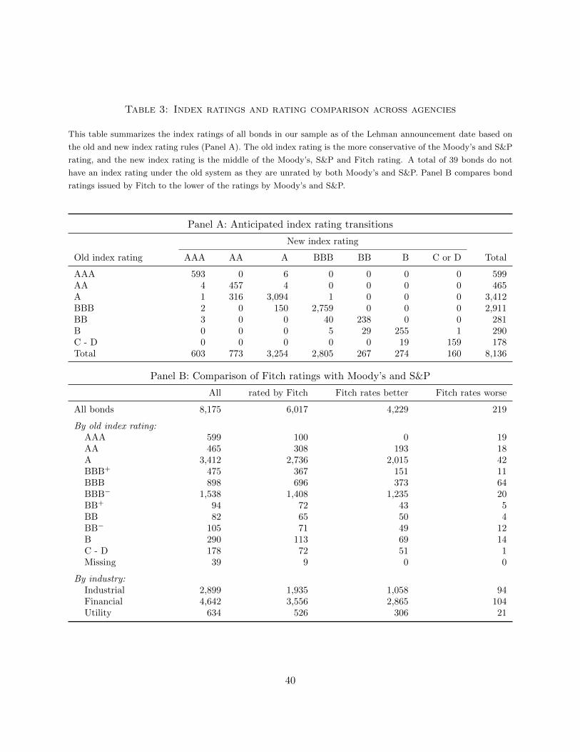
Table 3: Index ratings and rating comparison across agencies

This table summarizes the index ratings of all bonds in our sample as of the Lehman announcement date based on

the old and new index rating rules (Panel A). The old index rating is the more conservative of the Moody’s and S&P

rating, and the new index rating is the middle of the Moody’s, S&P and Fitch rating. A total of 39 bonds do not

have an index rating under the old system as they are unrated by both Moody’s and S&P. Panel B compares bond

ratings issued by Fitch to the lower of the ratings by Moody’s and S&P.

Panel A: Anticipated index rating transitions

New index rating

Old index rating AAA AA A BBB BB B C or D Total

AAA 593 0 6 0 0 0 0 599AA 4 457 4 0 0 0 0 465A 1 316 3,094 1 0 0 0 3,412BBB 2 0 150 2,759 0 0 0 2,911BB 3 0 0 40 238 0 0 281B 0 0 0 5 29 255 1 290C - D 0 0 0 0 0 19 159 178Total 603 773 3,254 2,805 267 274 160 8,136

Panel B: Comparison of Fitch ratings with Moody’s and S&P

All rated by Fitch Fitch rates better Fitch rates worse

All bonds 8,175 6,017 4,229 219

By old index rating:AAA 599 100 0 19AA 465 308 193 18A 3,412 2,736 2,015 42BBB+ 475 367 151 11BBB 898 696 373 64BBB− 1,538 1,408 1,235 20BB+ 94 72 43 5BB 82 65 50 4BB− 105 71 49 12B 290 113 69 14C - D 178 72 51 1Missing 39 9 0 0

By industry:Industrial 2,899 1,935 1,058 94Financial 4,642 3,556 2,865 104Utility 634 526 306 21

40

Table4:Abnormalreturnsforbondsupgraded

to

invest

mentgrade

This

table

rep

ort

scu

mula

tive

abnorm

al

retu

rns

for

the

sam

ple

of

30

upgra

ded

bonds

exp

ecte

dto

mov

eto

the

Leh

man

inves

tmen

t-gra

de

index

bec

ause

of

the

Leh

man

index

rati

ng

redefi

nit

ion.

Abnorm

al

retu

rns

are

calc

ula

ted

usi

ng

the

matc

hed

-sam

ple

appro

ach

des

crib

edin

Sec

tion

3.3

.T

he

contr

ol

gro

up

consi

sts

of

all

bonds,

matc

hed

on

index

rati

ng

and

matu

rity

,th

at

are

eith

ernot

rate

dby

Fit

chor

hav

ea

Fit

chra

ting

bel

owM

oody’s

and

S&

P.

Sp

ecifi

cally,

we

pair

bonds

base

don

thei

rold

Leh

man

index

rati

ng

up

toth

enotc

h.

Inaddit

ion,

we

matc

hon

bei

ng

inth

esa

me

matu

rity

bin

:sh

ort

(1-5

yea

rs)

or

long

(5yea

rsor

longer

).E

mpir

icalp-v

alu

esare

one-

sided

for

the

null

hyp

oth

esisH

0:CAR

t≤

0and

calc

ula

ted

usi

ng

the

boots

trap

pro

cedure

des

crib

ed

inSec

tion

3.3

.T

he

contr

ol

win

dow

abnorm

al

retu

rns

are

cum

ula

ted

over

the

pre

-announce

men

tp

erio

d(−

50,−

10]

and

are

use

das

ate

stof

whet

her

the

matc

hed

sam

ple

contr

ols

for

the

rele

vant

risk

chara

cter

isti

cs.

The

mark

er†

indic

ate

sth

eeff

ecti

ve

date

for

the

Leh

man

rule

change

(July

1,

2005),

and

t=

0re

fers

toth

eannounce

men

tdate

(Jan.

24,

2005).

The

even

tw

indow

abnorm

al

retu

rns

are

cum

ula

ted

start

ing

at

datet

=−

10,

and

the

hori

zons

in

the

firs

tco

lum

nare

inte

rms

of

tradin

gday

s.

HY

-to-

IG(M

ethod

1)

HY

-to-I

G(M

ethod

2)

HY

-to-I

G(S

hort

mat.

)H

Y-t

o-I

G(L

on

gm

at.

)T

ime

CA

Rp

CA

Rp

CA

Rp

CA

Rp

Con

trol

win

dow

:0.

30[0

.16]

0.4

2[0

.11]

0.5

7[0

.04]

0.2

7[0

.25]

Eve

nt

win

dow

:-5

0.56

[0.0

0]0.3

5[0

.05]

-0.2

0[0

.70]

0.9

1[0

.00]

01.

37[0

.00]

1.4

4[0

.00]

0.2

1[0

.28]

1.9

1[0

.00]

101.

58[0

.00]

1.6

7[0

.00]

-0.1

5[0

.65]

2.4

3[0

.00]

200.

86[0

.01]

0.9

5[0

.01]

-0.7

6[0

.97]

1.7

0[0

.00]

300.

81[0

.03]

0.8

4[0

.04]

-0.5

2[0

.91]

1.4

9[0

.00]

501.

26[0

.00]

1.0

6[0

.02]

0.6

0[0

.12]

1.4

9[0

.01]

802.

66[0

.00]

2.6

6[0

.00]

1.7

3[0

.05]

3.0

2[0

.01]

114†

2.96

[0.0

0]3.0

4[0

.00]

0.4

5[0

.25]

4.2

1[0

.00]

150

2.35

[0.0

0]2.5

3[0

.00]

0.3

7[0

.31]

3.2

7[0

.00]

200

1.50

[0.0

3]0.9

8[0

.11]

0.3

4[0

.33]

2.0

2[0

.02]

245

2.49

[0.0

0]1.9

5[0

.01]

0.6

1[0

.22]

3.4

0[0

.00]

41

Table5:Abnormalreturnsforbondsupgraded

to

invest

mentgrade—

robust

ness

This

table

rep

ort

scu

mula

tive

abnorm

al

retu

rns

for

the

30

upgra

ded

bonds

exp

ecte

dto

mov

eto

the

Leh

man

IGin

dex

.A

bnorm

al

retu

rns

are

calc

ula

ted

usi

ng

the

matc

hed

-sam

ple

appro

ach

des

crib

edin

Sec

tion

3.3

.T

he

contr

ol

gro

up

consi

sts

of

all

matc

hed

bonds

that

are

eith

ernot

rate

dby

Fit

chor

hav

e

aF

itch

rati

ng

bel

owM

oody’s

and

S&

P.

The

contr

ol

bonds

are

matc

hed

on

index

rati

ng,

matu

rity

,and

the

addit

ional

chara

cter

isti

cslist

edin

the

colu

mn

hea

der

s.Sp

ecifi

cally,

we

pair

bonds

base

don

thei

rold

Leh

man

index

rati

ng

up

toth

enotc

h(i

.e.,

BB

+,

BB

,B

B–,

B+

,et

c.)

and

two

matu

rity

bin

s(s

hort

:

1-5

yea

rsor

long:

5yea

rsor

longer

).In

dex

bet

as

for

the

IGin

dex

are

esti

mate

dusi

ng

Dim

son’s

met

hod

wit

hone

lead

and

lag

and

are

then

use

dto

defi

ne

terc

iles

bin

s(l

ess

than

0.0

6,

0.0

6-0

.569,

and

gre

ate

rth

an

0.5

69).

Liq

uid

ity

ism

easu

red

by

the

freq

uen

cyof

non-t

radin

gday

sand

then

terc

ile

bin

s

are

defi

ned

(les

sth

an

12%

,12-3

9%

,and

more

than

39%

).Is

sue

size

sare

gro

up

edin

tote

rcile

bin

sbase

don

par

valu

e(<

$150

MM

,$150–250

MM

,≥

$250

MM

).T

he

indust

ry-m

atc

hin

gis

base

don

thre

ebro

ad

sect

ors

(uti

lity

,financi

al,

and

indust

rial)

.E

mpir

icalp-v

alu

esare

one-

sided

for

the

null

hyp

oth

esis

H0

:CAR

t≤

0and

calc

ula

ted

usi

ng

the

boots

trap

pro

cedure

des

crib

edin

Sec

tion

3.3

.T

he

contr

ol

win

dow

abnorm

al

retu

rns

are

cum

ula

ted

over

the

pre

-announce

men

tp

erio

d(−

50,−

10]

and

are

use

das

ate

stof

whet

her

the

matc

hed

sam

ple

contr

ols

for

the

rele

vant

risk

chara

cter

isti

cs.

The

mark

er†

indic

ate

sth

eeff

ecti

ve

date

for

the

Leh

man

rule

change

(July

1,

2005),

andt

=0

refe

rsto

the

announce

men

tdate

(Jan.

24,

2005).

The

even

tw

indow

abnorm

al

retu

rns

are

cum

ula

ted

start

ing

at

datet

=−

10,

and

the

hori

zons

inth

efirs

tco

lum

nare

inte

rms

of

tradin

gday

s.

Ind

exb

eta

Liq

uid

ity

Issu

esi

zeC

ou

pon

Ind

ust

ryA

ll

Tim

eC

AR

pC

AR

pC

AR

pC

AR

pC

AR

pC

AR

p

Con

trol

win

dow

:0.

28[0

.19]

0.35

[0.1

4]

0.4

2[0

.08]

0.2

7[0

.17]

0.1

6[0

.28]

0.0

9[0

.40]

Eve

nt

win

dow

:-5

0.55

[0.0

0]0.

43[0

.01]

0.5

5[0

.00]

0.6

3[0

.00]

0.5

4[0

.00]

0.3

8[0

.01]

01.

07[0

.00]

1.27

[0.0

0]

1.4

2[0

.00]

1.5

2[0

.00]

1.4

3[0

.00]

1.6

0[0

.00]

101.

10[0

.00]

1.24

[0.0

0]

1.5

2[0

.00]

1.3

8[0

.00]

1.5

1[0

.00]

1.1

2[0

.00]

200.

55[0

.03]

0.67

[0.0

1]

0.8

8[0

.00]

0.7

3[0

.01]

0.8

1[0

.01]

0.8

1[0

.00]

300.

48[0

.12]

0.61

[0.0

6]

0.8

0[0

.02]

0.8

1[0

.03]

0.7

5[0

.05]

0.6

5[0

.06]

501.

11[0

.00]

1.28

[0.0

1]

1.4

0[0

.00]

1.2

1[0

.00]

1.2

5[0

.01]

1.3

4[0

.00]

802.

40[0

.00]

2.83

[0.0

0]

2.8

3[0

.00]

2.0

7[0

.01]

2.7

3[0

.00]

2.8

0[0

.00]

114†

2.62

[0.0

0]2.

91[0

.00]

2.9

5[0

.00]

2.5

9[0

.00]

2.8

0[0

.00]

2.4

9[0

.00]

150

1.96

[0.0

0]2.

30[0

.00]

2.4

0[0

.00]

2.0

8[0

.00]

2.0

9[0

.00]

1.7

5[0

.01]

200

1.38

[0.0

3]1.

54[0

.02]

1.5

9[0

.01]

1.2

4[0

.04]

1.3

3[0

.03]

1.5

0[0

.03]

245

2.36

[0.0

0]2.

34[0

.00]

2.4

3[0

.00]

2.2

6[0

.00]

2.4

1[0

.00]

2.3

5[0

.00]

42

Table 6: Decomposition of abnormal bond returns

The table reports estimates of the following decomposition of abnormal returns into a permanent component PCt

and a transitory component TCt for the 30 upgraded bonds expected to move to the Lehman IG index:

CARt = PCt + TCt,

PCt = PCt−1 + α1t0<t≤t1

t1 − t0+ β0 IMHt 1t>t1 + . . .+ βK IMHt−K1t>t1+K + ηt,

TCt = δ1TCt−1 + . . .+ δLTCt−L + εt,

where CARt is the cumulative abnormal return on the upgraded bond portfolio the matched-sample approach de-

scribed in Section 3.3, PCt is a unit root process, TCt is a mean-reverting process with zero long-run mean, IMHt is

the return on date t of a portfolio that is long the IG index and short the HY index, and 1 is an indicator that takes

value one during the time period indicated by the subscript, and zero otherwise. We choose t0 = −10 and t1 = 10.

The error terms (ηt, εt) are independent Gaussian random variables. We use the Kalman filter to estimate α, β, δ,

and PCt and TCt for t = 1, ..., T . Specifications (A), (B), and (C) vary the transitory lag length L. Specifications

(B), (D), and (E) vary the permanent lag length K.

(A) (B) (C) (D) (E)

α 1.50 1.44 1.44 1.45 1.45[0.01] [0.00] [0.00] [0.00] [0.00]

β0 0.19 0.19 0.19 0.16 0.16[0.00] [0.00] [0.00] [0.00] [0.00]

β1 0.07 0.07[0.10] [0.11]

β2 -0.01[0.82]

δ1 0.01 0.57 0.57 0.57 0.57[0.99] [0.00] [0.00] [0.00] [0.00]

δ2 0.18 0.18 0.20 0.21[0.02] [0.02] [0.01] [0.01]

δ3 -0.02[0.75]

σ2η 0.02 0.01 0.01 0.01 0.01

[0.00] [0.10] [0.08] [0.15] [0.15]σ2ε 0.01 0.03 0.03 0.03 0.03

[0.08] [0.00] [0.00] [0.00] [0.00]

Log-likelihood 59.33 62.60 62.65 67.36 66.71AIC -108.67 -113.20 -111.30 -120.72 -117.41BIC -90.44 -91.33 -85.78 -95.22 -88.31Observations 283 283 283 282 281

43

Table 7: Impact on bond trading activity

The table reports statistics on equally-weighted average daily turnover for the 30 upgraded bonds expected to move

to the Lehman IG index. There are three different event windows: the six-month window ending two weeks before the

announcement date (pre-announcement window), from two weeks before the announcement date to the effective date

(post-announcement window), and the six month window starting from the effective date to year-end (post-effective

window). The control sample comprises high-yield bonds with unfavorable or no Fitch rating. p-values are reported

in brackets. The Diff-in-Diff p-values are for Wald tests based on seemingly unrelated regressions (SUR) where the

errors are assumed to be serially independent but may have contemporaneous cross-equation correlations.

Event window Difference Diff-in-Diff

Pre- Post- Post- Post-ann. Post-eff. Post-ann. Post-eff.announce announce effective – Pre-ann. – Pre-ann. – Pre-ann. – Pre-ann.

Panel A: HY-to-IG bonds

Turnover (%) 0.26 0.54 0.37 0.28 0.11 0.27 0.16[0.00] [0.00] [0.00] [0.00] [0.09] [0.00] [0.00]

Panel B: HY bonds not rated favorably by Fitch (control sample)

Turnover (%) 0.30 0.31 0.25 0.01 -0.05 – –[0.00] [0.00] [0.00] [0.62] [0.04]

44

Tab

le8:

Bond

returnsand

orderflow

imbalances

This

table

giv

esre

sult

sfr

om

regre

ssio

ns

of

daily

retu

rns

on

ord

erflow

imbala

nce

sfo

rth

e30

upgra

ded

bonds

exp

ecte

dto

mov

eto

the

Leh

man

IGin

dex

.

The

dep

enden

tva

riable

isth

edaily

retu

rn.

InP

anel

Ath

eti

me

per

iod

isth

ep

ost

-announce

men

tw

indow

start

ing

two

wee

ks

bef

ore

the

announce

men

t

date

(January

24,

2005)

and

endin

gon

the

effec

tive

date

(July

1,

2005).

InP

anel

Bth

eti

me

per

iod

isth

ep

ost

-eff

ecti

ve

win

dow

start

ing

from

the

effec

tive

date

and

endin

gat

yea

r-en

d(D

ecem

ber

31,

2005).

We

show

esti

mati

on

resu

lts

for

both

poole

dO

LS

and

aver

age

coeffi

cien

tsfr

om

tim

e-se

ries

OL

Son

each

indiv

idual

bond.

To

com

pute

ord

erflow

imbala

nce

s,w

eco

mpare

the

transa

ctio

npri

ceof

each

trade

wit

hth

ecl

osi

ng

pri

ceon

the

most

rece

nt

pri

or

day

wit

htr

adin

g.

Ifth

etr

ansa

ctio

npri

ceis

hig

her

,w

ecl

ass

ify

the

transa

ctio

nas

abuy,

oth

erw

ise

as

ase

ll.

The

buy/se

llin

dic

ato

rsare

then

use

dto

com

pute

the

trade

dir

ecti

on

and

then

applied

tolo

gvolu

me

toco

mpute

ord

erflow

imbala

nce

s.p-v

alu

esare

show

nin

bra

cket

s.

Poole

dT

SP

oole

dT

SP

oole

dT

S

Pan

elA

:P

ost-

ann

oun

cem

ent

win

dow

(-10

,+

114]

–2,

133

obse

rvat

ion

s

Ord

erim

bal

ance

3.8

34.3

2[0

.00]

[0.0

0]

Ord

erfl

owim

bal

ance

(no.

trad

es)

34.8

748.1

9[0

.00]

[0.0

0]

Ord

erfl

owim

bal

ance

(no.

trad

es≥

$1M

M)

36.0

043.6

3[0

.00]

[0.0

0]

Vol

um

e2.9

71.6

03.8

82.8

24.2

63.5

4[0

.00]

[0.3

4]

[0.0

0]

[0.1

1]

[0.0

0]

[0.0

5]

R2

0.2

90.4

10.2

40.3

90.1

40.2

5

Pan

elB

:P

ost-

effec

tive

win

dow

(+11

4,+

245]

–2,

243

obse

rvat

ion

s

Ord

erim

bal

ance

3.4

03.9

0[0

.00]

[0.0

0]

Ord

erfl

owim

bal

ance

(no.

trad

es)

35.7

143.2

0[0

.00]

[0.0

0]

Ord

erfl

owim

bal

ance

(no.

trad

es≥

$1M

M)

34.6

041.3

8[0

.00]

[0.0

0]

Vol

um

e2.8

53.2

93.1

73.8

13.7

74.9

9[0

.00]

[0.0

1]

[0.0

0]

[0.0

0]

[0.0

0]

[0.0

0]

R2

0.2

60.3

80.2

40.3

60.1

10.1

8

45

Table9:In

surancecompa

nytrading

inbondssw

itching

from

HY

to

IGindex

The

table

rep

ort

sth

eeq

ual-

wei

ghte

dav

erage

net

purc

hase

sby

insu

rance

com

panie

sof

diff

eren

tty

pes

of

bonds

over

two

tim

ep

erio

ds.

The

trea

tmen

t

sam

ple

isth

e30

upgra

ded

bonds

exp

ecte

dto

mov

eto

the

Leh

man

IGin

dex

.In

Panel

Ath

eti

me

per

iod

isth

ep

ost

-announce

men

tw

indow

start

ing

two

wee

ks

bef

ore

the

announce

men

tdate

(January

24,

2005)

and

endin

gon

the

effec

tive

date

(July

1,

2005).

InP

anel

Bth

eti

me

per

iod

isth

ep

ost

-eff

ecti

ve

win

dow

start

ing

from

the

effec

tive

date

and

endin

gat

yea

r-en

d(D

ecem

ber

31,

2005).

Bond

class

ifica

tions

inea

chpanel

are

acc

ord

ing

tob

ond

rati

ngs

as

of

the

announce

men

tdate

.T

he

two

sets

of

colu

mns

mea

sure

insu

rance

com

pany

purc

hase

sin

dollar

term

sor,

resp

ecti

vel

y,as

fract

ion

of

issu

esi

ze.

The

firs

t

pair

of

colu

mn

inea

chse

tre

port

sth

eaggre

gate

change

inin

sura

nce

com

pany

hold

ings

by

rati

ng

cate

gory

,and

the

seco

nd

pair

rep

ort

sa

Diff

-in-D

iffte

stof

the

hyp

oth

esis

that

purc

hase

sof

upgra

ded

bonds

(tre

atm

ent

sam

ple

)are

not

larg

erth

an

those

of

bonds

inth

eco

rres

pondin

gco

ntr

ol

sam

ple

.T

hep-v

alu

es

are

for

Wald

test

sbase

don

seem

ingly

unre

late

dre

gre

ssio

ns

(SU

R)

wher

eth

eer

rors

are

ass

um

edto

be

seri

ally

indep

enden

tbut

may

hav

eco

nte

mp

ora

neo

us

cross

-equati

on

corr

elati

ons.

Thep-v

alu

esare

two-s

ided

for

the

diff

eren

cete

sts

and

one-

sided

for

the

Diff

-in-D

iffte

sts.

∆In

vento

ry($

MM

)∆

Inve

nto

ry(%

of

issu

e)

Diff

eren

ce[p

]D

iff-i

n-D

iff[p

]D

iffer

ence

[p]

Diff

-in

-Diff

[p]

Pan

elA

:P

ost-

ann

oun

cem

ent

win

dow

(-10

,+

114]

HY

-to-

IGb

ond

s6.

18[0

.21]

––

1.7

3[0

.29]

––

Con

trol

sam

ple

:B

ond

sn

otra

ted

favo

rab

lyby

Fit

ch,

spli

tby

ind

exra

tin

gA

AA

-A

-1.3

8[0

.05]

7.5

6[0

.07]

-0.9

8[0

.01]

2.7

1[0

.02]

BB

B+

-B

BB

-5.5

2[0

.00]

11.7

0[0

.02]

-2.2

2[0

.00]

3.9

5[0

.00]

BB

B–

-1.8

9[0

.38]

8.0

7[0

.07]

-0.4

5[0

.56]

2.1

8[0

.06]

BB

+-5

.37

[0.0

8]

11.5

5[0

.03]

-1.4

5[0

.42]

3.1

7[0

.02]

BB

-B

B–

-4.4

2[0

.00]

10.6

0[0

.02]

-1.0

9[0

.33]

2.8

2[0

.02]

B-1

.99

[0.0

2]

8.1

7[0

.06]

-0.6

6[0

.33]

2.3

8[0

.03]

Pan

elB

:P

ost-

effec

tive

win

dow

(+11

4,+

245]

HY

-to-

IGb

ond

s21

.29

[0.0

2]

––

3.9

6[0

.10]

––

Con

trol

sam

ple

:B

ond

sn

otra

ted

favo

rab

lyby

Fit

ch,

spli

tby

ind

exra

tin

gA

AA

-A

-6.0

9[0

.00]

27.3

8[0

.00]

-2.2

5[0

.00]

6.2

1[0

.00]

BB

B+

-B

BB

-4.7

4[0

.00]

26.0

3[0

.01]

-1.9

6[0

.01]

5.9

1[0

.00]

BB

B–

-7.9

4[0

.04]

29.2

3[0

.00]

-2.8

0[0

.02]

6.7

5[0

.00]

BB

+-7

.00

[0.2

8]

28.2

9[0

.01]

-2.4

7[0

.36]

6.4

3[0

.01]

BB

-B

B–

-4.9

6[0

.08]

26.2

5[0

.01]

-1.6

5[0

.31]

5.6

0[0

.00]

B-3

.21

[0.0

1]

24.5

0[0

.01]

-1.0

6[0

.29]

5.0

1[0

.00]

46

Table 10: Impact on liquidity

The table reports statistics on liquidity over three different event windows: the six-month window ending two weeks

before the announcement date (pre-announcement window), from two weeks before the announcement date to the

effective date (post-announcement window), and the six-month window starting from the effective date to year-end

(post-effective window). We compute Roll and Amihud liquidity measures for each bond separately and report

the cross-sectional average. See the text for further details. The treatment sample are the 30 upgraded bonds

expected to enter the Lehman IG index. The control sample comprises high-yield bonds with unfavorable or no

Fitch rating. p-values are reported in brackets. The Diff-in-Diff p-values are for Wald tests based on seemingly

unrelated regressions (SUR) where the errors are assumed to be serially independent but may have contemporaneous

cross-equation correlations.

Event window Difference Diff-in-Diff

Pre- Post- Post- Post-ann. Post-eff. Post-ann. Post-eff.announce announce effective – Pre-ann. – Pre-ann. – Pre-ann. – Pre-ann.

Panel A: HY-to-IG bonds

Liquidity (Roll) 1.27 1.13 1.17 -0.14 -0.10 -0.08 -0.06[0.00] [0.00] [0.00] [0.08] [0.27] [0.75] [0.68]

Liquidity (Amihud) 0.17 0.20 0.17 0.03 0.00 0.03 -0.01[0.00] [0.00] [0.00] [0.74] [0.95] [0.89] [0.57]

Panel B: HY bonds not rated favorably by Fitch (control sample)

Liquidity (Roll) 1.23 1.17 1.19 -0.06 -0.04 – –[0.00] [0.00] [0.00] [0.15] [0.36]

Liquidity (Amihud) 0.24 0.24 0.25 0.00 0.01 – –[0.00] [0.00] [0.00] [0.93] [0.94]

47

Table11:Reputationvs.

rating-induced

segmentation

The

table

rep

ort

scu

mula

tive

abnorm

al

retu

rns

for

all

bonds

rate

dfa

vora

bly

by

Fit

ch,

split

by

the

index

rati

ng

under

the

old

rule

.A

bnorm

al

retu

rns

are

calc

ula

ted

usi

ng

the

matc

hed

-sam

ple

appro

ach

des

crib

edin

Sec

tion

3.3

.T

he

contr

ol

gro

up

consi

sts

of

all

bonds,

matc

hed

on

index

rati

ng

and

matu

rity

,

that

are

eith

ernot

rate

dby

Fit

chor

hav

ea

Fit

chra

ting

bel

owM

oody’s

and

S&

P.

Sp

ecifi

cally,

we

pair

bonds

base

don

thei

rcr

edit

risk

by

matc

hin

gon

the

index

rati

ng

cate

gory

up

toth

enotc

hunder

Leh

man’s

old

split-

rati

ng

syst

em(i

.e.,

BB

+,

BB

,B

B–,

B+

,et

c.).

Inaddit

ion,

we

matc

hon

bei

ng

inth

esa

me

matu

rity

bin

:sh

ort

(1-5

yea

rs)

or

long

(5yea

rsor

longer

).E

mpir

icalp-v

alu

esare

one-

sided

for

the

null

hyp

oth

esisH

0:CAR

t≤

0and

calc

ula

ted

usi

ng

the

boots

trap

pro

cedure

des

crib

edin

Sec

tion

3.3

.T

he

contr

ol

win

dow

abnorm

al

retu

rns

are

cum

ula

ted

over

the

pre

-announce

men

tp

erio

d(−

50,−

10]

and

are

use

das

ate

stof

whet

her

the

matc

hed

sam

ple

contr

ols

for

the

rele

vant

risk

chara

cter

isti

cs.

The

mark

er†

indic

ate

sth

eeff

ecti

ve

date

for

the

rule

change,

andt

=0

refe

rsto

the

announce

men

tdate

.T

he

even

tw

indow

abnorm

al

retu

rns

are

cum

ula

ted

start

ing

at

datet

=−

10,

and

the

hori

zons

inth

efirs

t

colu

mn

are

inte

rms

of

tradin

gday

s.B

onds

issu

edby

GM

and

Ford

and

the

30

bonds

elig

ible

for

IGin

dex

incl

usi

on

(rep

ort

edin

Table

4)

are

excl

uded

from

this

analy

sis.

The

num

ber

of

trea

ted

bonds

inea

chco

lum

nis

rep

ort

edin

pare

nth

esis

.

Inve

stm

ent-

gra

de

bon

ds

Hig

h-y

ield

bon

ds

AA

A-

A(2

,180

)B

BB

+-

BB

B(5

15)

BB

B–

(247)

BB

+(1

8)

BB

-B

B–

(90)

B(6

4)

Tim

eC

AR

pC

AR

pC

AR

pC

AR

pC

AR

pC

AR

p

Con

trol

win

dow

:0.

37[0

.00]

-0.1

3[0

.90]

-0.0

7[0

.67]

0.7

1[0

.05]

0.1

3[0

.32]

-0.8

9[0

.98]

Eve

nt

win

dow

:-5

-0.2

7[1

.00]

-0.3

8[1

.00]

0.0

8[0

.16]

0.6

0[0

.00]

0.3

8[0

.04]

0.1

1[0

.25]

0-0

.32

[1.0

0]-0

.24

[1.0

0]

0.0

8[0

.23]

1.1

7[0

.00]

0.2

7[0

.09]

-0.3

1[0

.94]

10-0

.15

[1.0

0]-0

.36

[1.0

0]

0.3

5[0

.01]

1.4

0[0

.00]

0.2

7[0

.14]

0.2

4[0

.26]

20-0

.90

[1.0

0]-0

.27

[1.0

0]

-0.2

0[0

.90]

2.1

1[0

.00]

-0.0

7[0

.59]

0.8

3[0

.05]

30-0

.33

[1.0

0]-0

.37

[1.0

0]

-0.1

7[0

.80]

1.7

2[0

.00]

0.1

1[0

.31]

0.7

1[0

.06]

500.

04[0

.12]

0.30

[0.0

2]

-0.6

1[1

.00]

1.2

1[0

.01]

0.3

5[0

.13]

-0.0

6[0

.56]

80-0

.54

[1.0

0]0.

75[0

.00]

0.5

7[0

.01]

1.6

0[0

.11]

2.4

0[0

.00]

1.1

9[0

.04]

114†

-0.8

5[1

.00]

0.41

[0.0

1]

0.5

0[0

.05]

1.8

4[0

.02]

1.6

0[0

.00]

2.3

4[0

.00]

150

-0.8

9[1

.00]

0.27

[0.0

6]

0.4

1[0

.10]

1.4

4[0

.06]

1.1

4[0

.00]

2.4

2[0

.00]

200

-1.1

5[1

.00]

-0.1

8[0

.83]

0.0

0[0

.48]

2.5

3[0

.04]

1.7

9[0

.00]

1.5

1[0

.05]

245

-1.0

8[1

.00]

0.52

[0.0

1]

-0.0

3[0

.52]

2.7

7[0

.02]

0.6

1[0

.14]

1.8

5[0

.03]

48

Table 12: Abnormal stock returns and the Lehman announcement

The table reports estimation results on the cross-sectional variation in equity CARs around the Lehman announcement

date on stocks that are matched to bonds in our universe of 8,175 bonds. The regressors of interest are dummy

variables indicating the old Lehman rating category interacted with an indicator for a favorable Fitch rating. In

addition, the regression includes the old index rating dummy variables by themselves as controls for overall credit

risk and dummies for the company’s industry segment. p-values are shown in brackets.

(-10,+10] (-10,+30]

Coef. p Coef. p

AA × Fitch favorable 1.51 [0.25] 1.73 [0.30]A × Fitch favorable 0.32 [0.54] -0.77 [0.25]BBB+ - BBB × Fitch favorable 0.46 [0.46] -0.81 [0.31]BBB– × Fitch favorable 0.63 [0.36] -1.12 [0.29]BB+ × Fitch favorable 0.31 [0.89] 1.39 [0.64]BB - BB– × Fitch favorable 0.01 [0.99] 0.08 [0.96]B × Fitch favorable -0.47 [0.68] -1.41 [0.34]C - D × Fitch favorable 2.04 [0.36] 0.06 [0.98]No old index rating × Fitch favorable -0.35 [0.74] -3.30 [0.00]

AAA 0.26 [0.81] -1.12 [0.31]AA 0.20 [0.83] -0.63 [0.67]A 0.41 [0.47] -0.24 [0.73]BBB+ - BBB 0.31 [0.57] -0.05 [0.95]BBB– 0.01 [0.99] 0.15 [0.85]BB+ 0.76 [0.72] -0.76 [0.77]BB - BB– 0.33 [0.73] -0.39 [0.76]B 0.12 [0.87] 0.06 [0.95]C - D 1.14 [0.25] 0.75 [0.61]

Financial -1.49 [0.01] -1.88 [0.01]Industrial -0.18 [0.71] 0.53 [0.40]

Observations 561 561R2 0.02 0.04

49

Table 13: Abnormal returns for orphan bonds

The table reports cumulative abnormal returns for 18 bonds which were upgraded to an IG index rating but which were

not eligible for IG index inclusion. Abnormal returns are calculated using the matched-sample approach described

in Section 3.3. Panel A reports value-weighted CARs using the matched sample methodology. The control group

consists of all bonds, matched on index rating, maturity, and issue size category that are either not rated by Fitch

or have a Fitch rating below Moody’s and S&P. Specifically, we pair bonds based on their credit risk by matching on

the index rating category up to the notch under Lehman’s old split-rating system (i.e., BB+, BB, BB–, B+, etc.).

In addition, we match on being in the same maturity bin: short (1-5 years) or long (5 years or longer). Matching on

size is based on size terciles. Panel B reports cumulative returns for a portfolio that is long the 30 upgraded bonds

expected to move to the Lehman IG index and short the orphan bonds. Empirical p-values are one-sided for the

null hypothesis H0 : CARt ≤ 0 and calculated using the bootstrap procedure described in Section 3.3. The control

window abnormal returns are cumulated over the pre-announcement period (−50,−10] and are used as a test of

whether the matched sample controls for the relevant risk characteristics. The marker † indicates the effective date

for the rule change, and t = 0 refers to the announcement date. The event window abnormal returns are cumulated

starting at date t = −10, and the horizons in the first column are in terms of trading days.

HY index members (8) Index non-members (10) All orphaned bonds (18)

Time CAR p CAR p CAR p

Panel A: Long orphan bonds, short matched sample

Control window: 0.29 [0.31] -0.98 [1.00] -0.07 [0.59]

Event window:-5 1.18 [0.00] 0.06 [0.37] 0.75 [0.00]0 0.66 [0.06] -2.93 [1.00] -0.51 [0.96]10 1.86 [0.00] 2.11 [0.00] 1.88 [0.00]20 1.28 [0.02] -0.27 [0.60] 0.69 [0.07]30 1.21 [0.01] 1.24 [0.03] 1.22 [0.00]50 0.68 [0.24] 1.89 [0.00] 1.05 [0.06]80 2.84 [0.00] 5.81 [0.00] 4.00 [0.00]114† 4.22 [0.00] 6.34 [0.00] 5.15 [0.00]150 3.83 [0.00] 6.17 [0.00] 4.85 [0.00]200 3.13 [0.00] 2.19 [0.01] 3.02 [0.00]245 3.83 [0.01] 1.45 [0.03] 3.46 [0.00]

Panel B: Long HY-to-IG index bonds, short orphan bonds

Control window: 0.47 [0.00] 1.64 [0.01] 0.83 [0.01]

Event window:-5 -0.13 [0.66] -0.07 [0.64] -0.09 [0.61]0 0.68 [0.00] 2.80 [0.01] 1.30 [0.01]10 0.20 [0.30] -0.52 [0.86] 0.00 [0.48]20 -0.52 [0.83] -0.86 [0.92] -0.57 [0.82]30 -0.96 [0.90] -2.33 [1.00] -1.31 [0.94]50 -0.71 [0.97] -1.45 [1.00] -0.89 [0.98]80 -0.90 [1.00] 0.07 [0.50] -0.64 [0.91]114† -1.27 [0.92] 0.75 [0.12] -0.62 [0.70]150 -1.52 [0.95] -0.07 [0.55] -1.07 [0.84]200 -1.72 [0.96] 2.56 [0.10] -0.38 [0.61]245 -1.32 [0.91] 4.81 [0.00] 0.60 [0.34]

50

Table 14: Rating agency market shares before and after the Lehman announcement

The table reports the fraction of new corporate bond issues is rated by each rating agency. The pre-event period

covers the two years prior to the Lehman announcement, and the post-event period spans the two years following the

announcement. We restrict attention to ratings assigned within the first thirty days after issuance, and the data is

aggregated at monthly frequency. Panel A measures market penetration in terms of the dollar par value rated and

Panel B counts the number of issues rated as a fraction of all new issues. The column reports p-values for for tests

of the null hypothesis that market share declined (H0 : Post ≤ Pre).

Pre-event Post-event Post - Pre p-value forH0 : Post ≤ Pre

Panel A: Par value of new issues rated (%/100)

Fitch 0.45 0.56 0.11 [0.00]Moody’s 0.84 0.80 -0.04 [0.98]S&P 0.86 0.87 0.01 [0.26]

Panel B: Number of new issues rated (%/100)

Fitch 0.45 0.52 0.07 [0.00]Moody’s 0.86 0.78 -0.08 [1.00]S&P 0.90 0.87 -0.03 [0.99]

51

Figure 1: Index performance and timeline of events

The figure plots the cumulative return over time for the Lehman indices for investment-grade (IG) and high-yield

(HY) bonds normalized relative to the index level on November 15, 2004 (t = −50). The solid line plots the IG index

and the dashed line plots the HY index. The vertical dotted lines refer to important events in the corporate bond

market as described in Table 1. On the horizontal axis, 0 marks the announcement date (January 24, 2005) and 114

the effective date (July 1, 2005).

Ann

ounc

emen

t dat

e

Effe

ctiv

e da

te

GM

pro

fit w

arni

ng

GM

dow

ngra

de

GM

/For

d do

wng

rade

GM

dow

ngra

de

−10

−8

−6

−4

−2

02

Cum

ulat

ive

retu

rn (

%)

−50 0 50 100 150 200 250Time

Lehman IG IndexLehman HY Index

52

Figure 2: Announcement returns in bonds upgraded to investment grade

The figure plots value-weighted average cumulative abnormal returns for the 30 upgraded bonds expected to move

to the Lehman investment-grade index because of the Lehman index rating redefinition. Abnormal returns are

calculated using the matched-sample approach described in Section 3.3. The control group consists of all bonds,

matched on index rating and maturity, that are either not rated by Fitch or have a Fitch rating below Moody’s

and S&P. Specifically, we pair bonds based on their credit risk by matching on the index rating category up to the

notch under Lehman’s old split-rating rule (i.e., BB+, BB, BB–, B+, etc.). In addition, we match on being in the

same maturity bin: short (1-5 years) or long (5 years or longer). The dotted lines are the confidence interval at 95

percent significance level estimated using empirical p-values obtained using a bootstrap simulation procedure. On

the horizontal axis, 0 marks the announcement date (January 24, 2005) and 114 the effective date (July 1, 2005).

−1

01

23

45

Cum

ulat

ive

abno

rmal

ret

urn

(%)

−50 0 50 100 150 200 250Time

53

Figure 3: Announcement returns in bonds upgraded to investment grade—split bymaturity and turnover

The figure plots the cumulative returns on buy-and-hold bond portfolios comprising the 30 upgraded bonds expected

to move to the Lehman IG index. In Panel (a), the 30 upgraded bonds are classified into two sub-samples based on

their maturity. The solid line refers to the sample with long maturity (5 years or longer), and the dashed line to the

short maturity sample (1-5 years). In Panel (b), the 30 upgraded bonds are classified into three sub-samples based

on their turnover over the post-event window (0,+30], with one third of bonds in each sub-sample. The solid line

refers to the sample with high turnover (top tercile), the dashed line to the medium turnover sample (middle tercile),

and the dotted line to the low turnover sample of bonds (bottom tercile). Date t = 0 refers to the announcement on

January 24, 2005.

−1

01

23

45

Cum

ulat

ive

retu

rn (

%)

−10 0 10 20 30Time

short maturitylong maturity

(a) Returns on bonds upgraded to IG—split by maturity

−1

01

23

45

Cum

ulat

ive

retu

rn (

%)

−10 0 10 20 30Time

low turnovermedium turnoverhigh turnover

(b) Returns on bonds upgraded to IG—split by turnover54

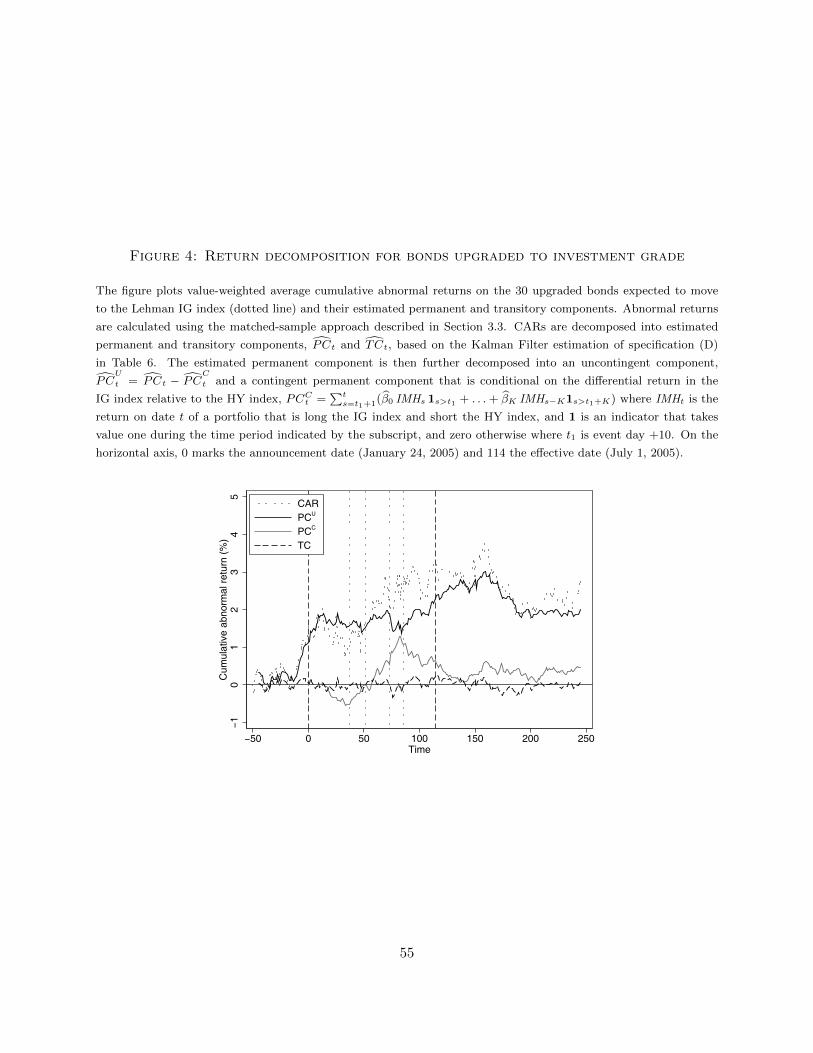
Figure 4: Return decomposition for bonds upgraded to investment grade

The figure plots value-weighted average cumulative abnormal returns on the 30 upgraded bonds expected to move

to the Lehman IG index (dotted line) and their estimated permanent and transitory components. Abnormal returns

are calculated using the matched-sample approach described in Section 3.3. CARs are decomposed into estimated

permanent and transitory components, PCt and TCt, based on the Kalman Filter estimation of specification (D)

in Table 6. The estimated permanent component is then further decomposed into an uncontingent component,

PCU

t = PCt − PCC

t and a contingent permanent component that is conditional on the differential return in the

IG index relative to the HY index, PCCt =

∑ts=t1+1(β0 IMHs 1s>t1 + . . .+ βK IMHs−K1s>t1+K) where IMHt is the

return on date t of a portfolio that is long the IG index and short the HY index, and 1 is an indicator that takes

value one during the time period indicated by the subscript, and zero otherwise where t1 is event day +10. On the

horizontal axis, 0 marks the announcement date (January 24, 2005) and 114 the effective date (July 1, 2005).

−1

01

23

45

Cum

ulat

ive

abno

rmal

ret

urn

(%)

−50 0 50 100 150 200 250Time

CARPCU

PCC

TC

55

Figure 5: Post-announcement turnover in bonds upgraded to investment grade

The figure reports the equally-weighted average daily turnover for the 30 upgraded bonds expected to move to the

Lehman IG index (solid line). Turnover is calculated as the dollar volume of all transactions reported in TRACE

and normalized by the outstanding par value. The control sample (dashed line) comprises high-yield bonds with

unfavorable or no Fitch rating. On the horizontal axis, 0 marks the announcement date (January 24, 2005) and 114

the effective date (July 1, 2005).

0.2

.4.6

.8T

urno

ver

(%)

−50 0 50 100 150 200 250Time

HY−to−IGControl sample

56

Figure 6: Insurance company trading in bonds switching from HY to IG index

The figure plots the equal-weighted average cumulative change in the aggregate insurance company holdings of the

30 upgraded bonds expected to move to the Lehman IG index (in units of $ MM per bond). The dashed line plots

the corresponding average change in inventory for bonds in the control sample of matched bonds. On the horizontal

axis, 0 marks the announcement date (January 24, 2005) and 114 the effective date (July 1, 2005).

−10

010

20C

hang

e in

insu

ranc

e ho

ldin

gs (

$ M

M)

−50 0 50 100 150 200 250Time

HY−to−IGControl sample

57

Figure 7: Upgraded GM and Ford bonds around Lehman announcement date

Panel (a) plots the average daily turnover in GM, GMAC, Ford, and FMCC bonds around the announcement

date. Turnover is measured using TRACE transactions volume data and normalized by the par amount outstanding

(obtained from FISD). Panel (b) plots the cumulative returns of bonds issued by GM, GMAC, Ford, and FMCC

around the announcement date. All of these bonds have a BBB– rating issued from Standard and Poor’s and a

rating of BBB or BBB+ from Fitch. The sample consists of 984 bonds and is split according to the credit rating

issued by Moody’s into A– (farthest from HY), BBB+, and BBB (closest to HY). On the horizontal axis, 0 marks

the announcement date (January 24, 2005).

02

46

8T

urno

ver

(%)

−20 −10 0 10 20Time

Moody’s BBBMoody’s BBB+Moody’s A−

(a) Turnover

−5

−4

−3

−2

−1

01

Cum

ulat

ive

retu

rn (

%)

−20 −10 0 10 20Time

(b) Announcement returns

58

Internet Appendix

Appendix C. Cross-sectional Regression and Control Variables

Cross-sectional regressions are used to verify that the differences in returns across the treated bondsand the control sample are not due to bond characteristics that vary systematically across theseportfolios. The cross-sectional approach allows us to simultaneously estimate the abnormal returnson multiple sub-samples of interest. We run regressions of the following form:

CRi = α+∑k

βkIi,k + γ′Xi + εi,

where the cumulative raw return CRi for bond i is regressed on two types of explanatory variables.The first regressors are a set of indicator variables Ii,k, k = 1, . . . ,K for a set of K subsamples, thattake on a value of one if bond i is in sub-sample k, and zero otherwise. The coefficient βk on Ii,kyields an estimate for the mean CAR on sub-sample k. The second regressors are a set of controlvariables Xi that have been used in the literature to explain bond returns:

• Maturity: maturity of bond i in years;

• Age: age of bond i, measured in years since offering date;

• Coupon: measured in percent;

• Issue size: Dummies for the par amount of the bond outstanding, split into five ranges: (0, 50),[50, 150), [150, 250), [250, 1, 000), [1, 000,∞) in $MM.

• Credit risk: dummies for the rating under the old rule: AAA, AA, A, BBB/BBB+, BBB−,BB+, BB/BB−, B, C - D and bonds unrated by Moody’s and S&P, or a coarser definition(AAA - A, BBB, BB, B, etc.);

• Dummies for the industry group: Industrial, Financial, Utility.

To address measurement problems due to infrequent trading, we compute returns by averagingtransaction prices over consecutive days. We use the volume-weighted average “clean” price over[t0 − L, t0] as the pre-event price and the volume-weighted “clean” price over [t1, t1 + L] as thepost-event price when computing the cumulative return over the time period [t0, t1]. For most ofthe analysis, we choose L = 3. Cumulative returns are then computed as the percentage differencebetween post-event and pre-event bond prices: CR[t0,t1] = ln(P t1,t1+L)− ln(P t0−L,t0).

59

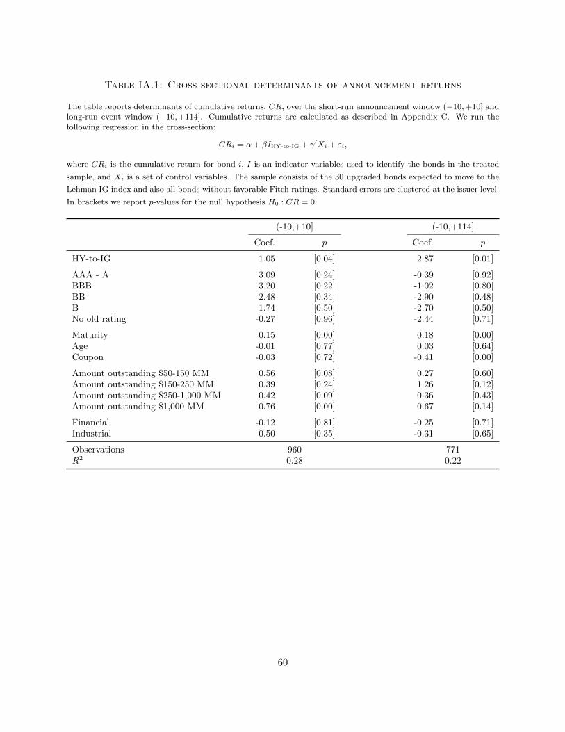
Table IA.1: Cross-sectional determinants of announcement returns

The table reports determinants of cumulative returns, CR, over the short-run announcement window (−10,+10] andlong-run event window (−10,+114]. Cumulative returns are calculated as described in Appendix C. We run thefollowing regression in the cross-section:

CRi = α+ βIHY-to-IG + γ′Xi + εi,

where CRi is the cumulative return for bond i, I is an indicator variables used to identify the bonds in the treated

sample, and Xi is a set of control variables. The sample consists of the 30 upgraded bonds expected to move to the

Lehman IG index and also all bonds without favorable Fitch ratings. Standard errors are clustered at the issuer level.

In brackets we report p-values for the null hypothesis H0 : CR = 0.

(-10,+10] (-10,+114]

Coef. p Coef. p

HY-to-IG 1.05 [0.04] 2.87 [0.01]

AAA - A 3.09 [0.24] -0.39 [0.92]BBB 3.20 [0.22] -1.02 [0.80]BB 2.48 [0.34] -2.90 [0.48]B 1.74 [0.50] -2.70 [0.50]No old rating -0.27 [0.96] -2.44 [0.71]

Maturity 0.15 [0.00] 0.18 [0.00]Age -0.01 [0.77] 0.03 [0.64]Coupon -0.03 [0.72] -0.41 [0.00]

Amount outstanding $50-150 MM 0.56 [0.08] 0.27 [0.60]Amount outstanding $150-250 MM 0.39 [0.24] 1.26 [0.12]Amount outstanding $250-1,000 MM 0.42 [0.09] 0.36 [0.43]Amount outstanding $1,000 MM 0.76 [0.00] 0.67 [0.14]

Financial -0.12 [0.81] -0.25 [0.71]Industrial 0.50 [0.35] -0.31 [0.65]


60

Table IA.2: Determinants of announcement returns on bonds issued by GM and Ford

The table reports estimates for the cross-sectional determinants of cumulative returns around the announcement date

for bonds issued by GM and Ford. Estimation results are from a cross-sectional regression on cumulative returns

over different horizons. p-values are shown in brackets.

[-1,+10] [-1,+20]

Coef. p Coef. p

Moody’s BBB 1.64 [0.02] 1.38 [0.01]Moody’s BBB+ 0.83 [0.04] 1.03 [0.00]

Maturity 0.11 [0.06] 0.05 [0.16]Age 0.05 [0.57] 0.06 [0.50]Coupon 0.29 [0.30] 0.04 [0.85]

Amount outstanding $50-150 MM 0.22 [0.47] 0.49 [0.12]Amount outstanding $150-250 MM -1.07 [0.08] -1.75 [0.02]Amount outstanding $250-1,000 MM -0.23 [0.76] -0.12 [0.81]Amount outstanding ≥$1,000 MM 1.43 [0.00] 1.18 [0.00]


61

Table IA.3: Reputation vs. rating-induced segmentation: Short-run announcementreturns

The table reports cumulative returns, CR, over the short-run event window (−10,+10] for value-weighted samples

of bonds split by the old segment (Panel A) and old index rating (Panel B) and the respective Fitch rating status.

The column Difference fav. – not fav. reports the return difference between bonds rated favorably by Fitch (that is,

bonds with Fitch rating higher quality than Moody’s and S&P) and bonds not rated favorably (that is, bonds with

Fitch rating of lower quality than Moody’s and S&P or not rated by Fitch). The column Diff-in-diff reports the

difference between the HY and IG segment (Panel A) or between BB+ and BBB– (Panel B) in the return difference

between bonds rated favorably versus not rated favorably by Fitch. In brackets we report p-values for the one-sided

alternative Ha : CR(−10,+10] ≥ 0.

Panel A: Split by segment

Fitch favorable Fitch not favorable Difference Diff-in-diff

Obs. CR p Obs. CR p fav. – not fav. HY – IG

IG 2,247 0.84 [0.00] 1,399 0.79 [0.00] 0.05 [0.30]HY 191 1.14 [0.00] 236 0.33 [0.03] 0.81 [0.00] 0.76 [0.00]

Panel B: Split by index rating

Fitch favorable Fitch not favorable Difference Diff-in-diff

Obs. CR p Obs. CR p fav. – not fav. BB+ – BBB–

IG by rating:AAA - AA- 128 0.34 [0.01] 533 0.69 [0.00] -0.35 [0.94]A+ - A- 1,479 0.79 [0.00] 443 0.74 [0.00] 0.05 [0.36]BBB+ 128 1.16 [0.00] 92 0.76 [0.00] 0.40 [0.10]BBB 292 1.04 [0.00] 209 1.14 [0.00] -0.10 [0.65]BBB– 220 0.98 [0.00] 122 0.64 [0.00] 0.34 [0.04]

HY by rating:BB+ 41 2.07 [0.00] 26 0.75 [0.02] 1.32 [0.01] 0.98 [0.04]BB 44 0.99 [0.00] 13 0.74 [0.04] 0.25 [0.31]BB– 44 0.73 [0.00] 42 0.70 [0.01] 0.03 [0.48]B+ - B– 62 0.85 [0.01] 155 0.12 [0.31] 0.73 [0.05]

62

Figure IA.1: Trading frequency

This figure plots the frequency of trading over the time period (−50,+245]. Panel (a) is for the 30 upgraded bonds

expected to move the the Lehman IG index, and panel (b) is for the control bonds.

0.2

.4.6

.8F

ract

ion

of tr

ades

1 2 3 4 5 6 7 8 9 10 11 12 13 14 15Time between trades

(a) HY-to-IG

0.2

.4.6

.8F

ract

ion

of tr

ades

1 2 3 4 5 6 7 8 9 10 11 12 13 14 15Time between trades

(b) Control sample

Figure IA.2: Bond returns and order flow imbalances

This figure plots the actual (solid) and predicted (dashed) average cumulative abnormal returns for the 30 upgraded

bonds expected to move to the Lehman IG index. The predictions are obtained from the regression of daily returns

on order flow imbalances and volume in Table 8.

−1

01

23

45

Cum

ulat

ive

abno

rmal

ret

urns

(%

)

−50 0 50 100 150 200 250Time

63

Documents

Why Ratings Matter: Evidence from the Lehman Brothers ... · Why Ratings Matter: Evidence from the Lehman Brothers Index Rating Rede nition Zhihua Chen Aziz A. Lookman Norman Schurho