Why do linear SVMs trained on HOG features perform so well?

Hilton Bristow1 and Simon Lucey21Queensland University of Technology, Australia

2Carnegie Mellon University, USA

Abstract

Linear Support Vector Machines trained on HOGfeatures are now a de facto standard across many visualperception tasks. Their popularisation can largely be at-tributed to the step-change in performance they broughtto pedestrian detection, and their subsequent successesin deformable parts models. This paper explores the in-teractions that make the HOG-SVM symbiosis performso well. By connecting the feature extraction and learn-ing processes rather than treating them as disparate plu-gins, we show that HOG features can be viewed as doingtwo things: (i) inducing capacity in, and (ii) addingprior to a linear SVM trained on pixels. From thisperspective, preserving second-order statistics and lo-cality of interactions are key to good performance. Wedemonstrate surprising accuracy on expression recogni-tion and pedestrian detection tasks, by assuming onlythe importance of preserving such local second-order in-teractions.

1. Introduction

Despite visual object detectors improving by leapsand bounds in the last decade, they still largelyrely on the same underlying principles: linear Sup-port Vector Machines (SVMs) trained on Histogramof Oriented Gradient (HOG) features. When HOGfeatures were introduced, they improved upon exist-ing methods for pedestrian detection by an order ofmagnitude [5]. Since then, the HOG-SVM pipelinehas been used in the deformable parts model of [9],its derivatives, and high achievers of the PASCALVOC challenge. A keyword search for “HOG” and“SVM” in the PASCAL 2012 results page returns 25and 18 hits respectively. HOG is now complicit indetection pipelines across almost every visual detec-tion/classification task [5, 7, 20, 21].

In this paper we peel back the layers of complex-ity from HOG features to understand what underlyinginteractions drive good performance. In particular,

• HOG features can be viewed as an affine weightingon the margin of a quadratic kernel SVM,

• underlying this prior and added capacity is thepreservation of local pixel interactions and second-order statistics,

• using these foundational components alone, weshow it is possible to learn a high performingclassifier, with no further assumptions on images,edges or filters.

2. Representing HOG features as a lineartransform of pixels

HOG features can be described as taking a nonlinearfunction of the edge orientations in an image and pool-ing them into small spatial regions to remove sensitivityto exact localisation of the edges. A pictorial represen-tation of this pipeline is shown in Figure 1. This typeof representation has proven particularly successful atbeing tolerant to non-rigid changes in object geometrywhilst maintaining high selectivity [8].

The exact choice of non-linear function is discre-tionary, however Dalal and Triggs try f(x) = |x| andf(x) = |x|2. Both functions remove the edge direction,leaving only a function of the magnitude. In this pa-per, we choose to use the square of edge directions. Ourchoice is motivated by a number of reasons. First, thesquare function leads to greater flexibility in manipu-lation, which we show becomes vital in our later refor-mulation. Second, there are proponents of the squaringfunction (referred to as “square” or “L2” pooling) inconvolutional network literature [1, 14], whose archi-tectures have a similar pipeline to HOG features perlayer, and have shown exciting results on large-scalevisual recognition challenges [16]. Finally, the squarefunction has a good basis in statistical models of theprimary visual cortex [13].

Following the notation of [3], the transform frompixels to output in HOG features can be written as,

Φf (x) = Db ∗ [(gf ∗ x)� (gf ∗ x)] , (1)

1

arX

iv:1

406.

2419

v1 [

cs.C

V]

10

Jun

2014

Weighted vote into spatial and

orientation binsInput image Compute gradients

Nonlinear transform

Contrast normalize Linear SVM

�f (x) = Db ⇤ [(gf ⇤ x) � (gf ⇤ x)]Figure 1. An illustration of the HOG feature extraction process and how each component maps to our reformulation.Gradient computation is achieved through convolution with a bank of oriented edge filters. The nonlinear transform isthe pointwise squaring of the gradient responses which removes sensitivity to edge contrast and increases edge bandwidth.Histogramming can be expressed as blurring with a box filter followed by downsampling.

where a vectorized input image x ∈ RD is convolvedwith an oriented edge filter gf [6], rectified throughthe Hadamard operator (pointwise square), then finallyblurred with b and downsampled by the sparse selec-tion matrix D to achieve pooling/histogramming. Per-forming this operation over a bank of oriented edge fil-ters and concatenating the responses leads to the finaldescriptor,

Φ(x) = [Φ1(x) Φ2(x) . . . ΦF (x)] . (2)

This reformulation omits the contrast normalizationstep, which we address later in the piece. We showedpreviously in [3] that each sub-descriptor can be ex-pressed in the form,

Φf (x) = DBM(Gf ⊗Gf )(x⊗ x) , (3)

where M is a selection matrix and capitalized B, G arematrix forms of their convolutional prototypes. Thefull response to a bank of filters can be written as,

Φ(x) = L(x⊗ x) , (4)

where the projection matrix L is formed by concate-nating the bank,

L =

BM(G1 ⊗G1)...

BM(GF ⊗GF )

. (5)

Under this reformulation, HOG features can beviewed as an affine weighting of quadratic interactionsbetween pixels in the image. This suggests that thegood performance of HOG features is down to twothings: (i) second-order interactions between pixels,and (ii) the choice of prior that forms the affine weight-ing L.

3. Capacity of the Classifier

When used in a support vector classification set-ting, the projection matrix L can be absorbed into the

margin,

w∗ = arg minw,ξi≥0

1

2wT (LTL)−1w + C

l∑i=1

ξi (6)

subject to yiwT (xi ⊗ xi) > 1− ξi, i = 1 . . . l

leaving as the data term only interactions between theweights w and the Kronecker expansion of the image.

Remark 1 When the weighting is the identity matrix,( i.e. L = I), Equation (6) reduces to an SVM with aunary quadratic kernel.

The first part of the HOG story, the induced prior,can thus be quantified as being quadratic. The weight-ing matrix is therefore intrinsically a prior on the mar-gin of a quadratic kernel SVM.

4. Secord-Order Interactions

The term (x⊗ x) in Equation (4) can alternativelybe written as,

(x⊗ x) = vec(xxT ) , (7)

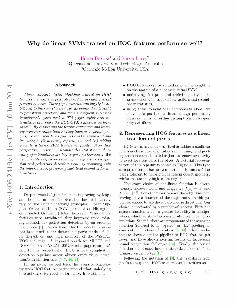
which is the vectorized covariance matrix of all pixelinteractions. [19] showed that the covariance of a localimage distribution is often enough to discriminate itfrom other distributions. However, when dealing withhigh-dimensional distributions, computing a full-rankcovariance matrix is often difficult. [10] circumvent thisproblem by assuming stationarity of background im-age statistics (a translated image is still an image), aswell as limiting the bandwidth of interactions betweenpixels. Simoncelli [18] showed that these assumptionsare reasonable, since correlations between pixels fallquickly with distance (see Figure 2).

To improve conditioning and prevent overfitting theclassifier to hallucinated interactions, we consider themost general set of local second-order features: the setof all local unary second-order interactions in an image,

Ψ(x) = [vec{S1(x)}T , . . . , vec{SD(x)}T ]T (8)

2

0 100 2000

50

100

150

200

250

I(x,y)

I(x+

1,y

+1

)

0 100 2000

50

100

150

200

250

I(x,y)

I(x+

2,y

+2

)

0 100 2000

50

100

150

200

250

I(x,y)

I(x+

5,y

+5

)

0 100 2000

50

100

150

200

250

I(x,y)

I(x+

10

,y+

10

)

Figure 2. An illustration of the locality of pixel correlations in natural images. Whilst a single pixel displacment exhibitsstrong correlations in intensity, there are few discernible correlations beyond a 5 pixel displacement. Locality is also observedin the human visual system, where cortical cells have finite spatial receptive fields.

where,

Si(x) = PixxTPTi , (9)

Pi is simply an M × D matrix that extracts an Mpixel local region centred around the ith pixel of theimage x. By retaining local second-order interactions,the feature length grows from D for raw pixels to M2D.

Fortunately, inspection of Equation (8) reveals alarge amount of redundant information. This redun-dancy stems from the re-use of pixel interactions insurrounding local pixel locations. Taking this into ac-count, and without loss of information, one can com-pact the local second-order feature to MD elements,so that Equation (8) becomes,

Ψ∗(x) =

(e1 ∗ x)T ◦ xT...

(eM ∗ x)T ◦ xT

. (10)

where {em}Mm=1 is the set of M impulse filters thatencode the local interactions in the signal.

5. Local Second-Order Interactions

Consider two classes A and B. Class A represents thedistribution of all natural images. Class B represents anoise distribution which has the same frequency spec-trum as natural images, namely 1

f [18]. Both distribu-tions are power normalized. We sample 25000 train-ing and testing examples from each class, and traintwo classifiers: one preserving the raw pixel informa-tion and one preserving local second-order interactionsof the pixels. The goal of the classifiers is to predict“natural” or “noise.” An illustration of the experi-mental setup and the results are presented in Figure3. The pixel classifier fails to discriminate betweenthe two distributions. There is no information in ei-ther the spatial or Fourier domain to linearly separatethe classes (i.e. the distributions overlap). By preserv-ing local quadratic interactions of the pixels, however,

the classifier can discriminate natural from syntheticalmost perfectly.

Whilst the natural image and noise distributionshave the same frequency spectra, natural images arenot random: they contain structure such as lines, edgesand contours. This experiment shows that image struc-ture is inherently local, and more importantly, that lo-cal second-order interactions of pixels can exploit thisstructure. Without encoding an explicit prior on edges,pooling, histogramming or blurring, local quadratic in-teractions have sufficient capacity to exploit the statis-tics of natural images, and separate them from noise.

6. Replacing prior with posterior:learning over pixels

Quadratic kernel SVMs have not historically per-formed well on recognition tasks when learned usingpixel information. The image prior that HOG encodes,and the affine weighting that it can be distilled into, isintegral to obtaining good generalisation performance.We know, however, that a prior is simply used to reflectour belief in the posterior distribution in the absenceof actual data. In the case of HOG, the prior encodesinsensitivity to local non-rigid deformations so that theentire space of deformation does not need to be sam-pled to make informed decisions.

This is usually a reasonable assumption to make,since sampling the posterior sufficiently may be infea-sible. Take, for example, the task of pedestrian detec-tion. The full posterior comprises all possible combina-tions of pose, clothing, lighting, race, gender, identity,background and any other attribute that manifests ina change to the visual appearance of a person. Multi-scale sliding window HOG detectors (with pose elastic-ity in the case of DPMs) work to project out as muchof this intra-class variation as possible.

Is it possible to learn a detector using only the as-sumptions that underlie HOG features: the preserva-tion of local second-order interactions? How much data

3

1

f

1

f

(a) (b) (c)pixels local quadratic

chance(50%)

52.6%

99.3%

|F(x)| |F(x)|

Figure 3. Thought-experiment setup. (a) contains an ensemble of samples drawn from the space of natural images witha 1

ffrequency spectrum, (b) contains an ensemble of samples drawn from a random noise distribution with the same 1

f

frequency spectrum. (c) We train two linear classifiers to distinguish between “natural” or “noise.” The pixel-based classifierdoes not have the capacity to discriminate between the distributions. The classifier which preserves local quadratic pixelinteractions almost perfectly separates the two distributions.

is required to render the HOG prior unnecessary, andwhat sort of data is required? Can the data just beperturbations of the training data? Does the result-ing classifier learn anything more specialized than onelearned on HOG features? In the following section weaim to provide answers to these questions.

Hypothesis 1 If HOG features are doing what we in-tend - providing tolerance to local geometric misalign-ment - then it should be possible to reproduce their ef-fects by sampling from a sufficiently large dataset con-taining geometrically perturbed instances of the originaltraining set.

Learned Features: It is the firm belief of many thatlearned features are the way forward [11]. Convolu-tional network literature has heavily relied on learnedfeatures for a number of years already [15, 17]. Wetake feature learning to its most primitive form, set-ting only the capacity and distribution of features, andletting the classifier learn the rest.

7. Methods

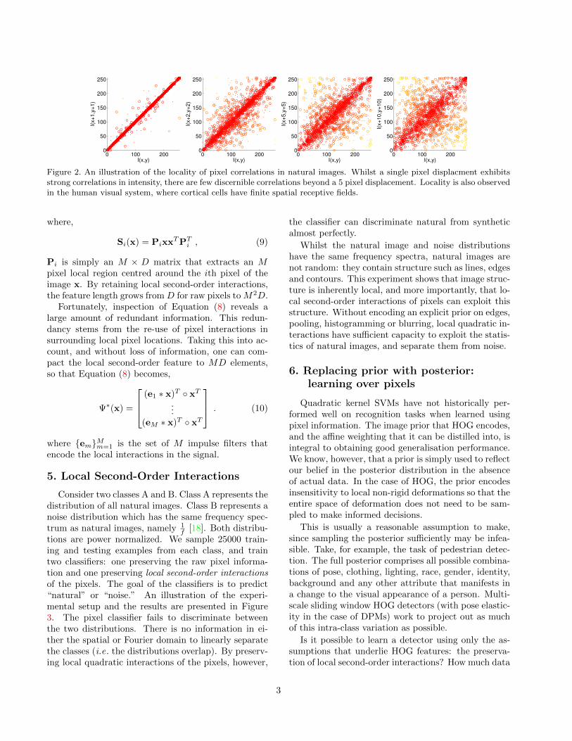
We designed an experiment where we could controlthe amount of geometric misalignment observed be-tween the training and testing examples. We used theCohn Kanade+ expression recognition dataset, consist-ing of 68-point landmark, broad expression and FACS

labels across 123 subjects and 593 sequences. Each se-quence varies in length and captures the neutral andpeak formation of facial expression. In this paper weconsider only the task of broad expression classifica-tion (i.e. we discard FACS encodings). To test theinvariance of different types of features to geometricmisalignment, we first register each training exampleto a canonical pose, then synthesize similarity warps ofthe examples with increasing RMS point error.

Why Faces?: HOG features have been used acrossa broad range of visual recognition tasks, includingobject recognition, scene recognition, pose estimation,etc. Faces are unique, however, since they are a heav-ily studied domain with many datasets containing sub-jects photographed under controlled lighting and poseconditions, and labelled with ground-truth facial land-marks. This enables a great degree of flexibility inexperimental design, since we can programatically setthe amount of geometric misalignment observed whilecontrolling for pose, lighting, expression and identity.

We synthesize sets with 300, 1500, 15000 and 150000training examples. The larger the synthesized set, thegreater the coverage of geometric variation. We useHOG features according to Felzenszwalb et al . [9] with18 orientations and a spatial aggregation size of 4. Forthe reformulation of Equation (2), we use Gabor fil-ters with 18 orientations at 4 scales, and a 4 × 4 blurkernel. The local quadratic features have a spatial sup-

4

(a) 0-pixel error

(b) 10-pixel errorFigure 4. Illustrative examples of subjects from the CohnKanade+ dataset with (a) zero registration error, and (b)10 pixels of registration error.

port equal to the amount of RMS point error (i.e. at10 pixels error, correlations are collected over 10 × 10regions). All training images are 80 × 80 pixels andcropped around only the faces. Figure 4 illustrates thedegree of geometric misalignment introduced.

Contrast Normalization: So far we have neglectedto mention contrast normalization, the final stage inthe HOG feature extraction pipeline, and a componentthat has traditionally received much attention, partic-ularly in neuroscience literature [4]. Whilst contrastnormalization is an integral part of HOG features, wedo not believe it plays a significant role in their invari-ance to geometry. Since our model does not explainthe highly nonlinear process of contrast normalization,we instead power normalize images in the expressionrecognition experiment, and pre-whiten images in thepedestrian detection experiment.

Learning: The storage requirements of local quadraticfeatures quickly explode with increasing geometric er-ror and synthesized examples. At 10 pixels RMS error,150000 training examples using local quadratic featurestakes 715 GB of storage. To train on such a largeamount of data, we implemented a parallel support vec-tor machine [2] with a dual coordinate descent methodas the main solver [12]. Training on a Xeon server us-ing 4 cores and 24 GB of RAM took between 1 – 5days, depending on problem size. We used multiplemachines to grid search parameters and run differentproblem sizes.

Figure 5 shows a breakdown of the results for syn-thesized sets of geometric variation. Pixels (shown inshades of green) perform consistently poorly, even withlarge amounts of data. HOG features (in blue, and re-formulation in aqua) consistently perform well. Theperformance of HOG saturates after just 1500 trainingexamples. [23] talk about the saturation of HOG atlength, noting that more data sometimes decreases itsperformance.

Local quadratic features (shown in red) have amarked improvement in performance with increasingamounts of data (roughly 10% per order of magnitude

of training data). Synthesizing variation used to bequite popular in some vision circles, particularly facerecognition through the use of AAMs [22], however itseems to have gone out of fashion in object recognition.Our results suggest that a model with sufficient capac-ity could benefit from synthesized data, even on generalobject recognition tasks (see Pedestrian Detection).

Only when the dataset contains ≥ 100000 exam-ples do the local quadratic features begin to modelnon-trivial correlations correctly. With 150000 trainingsamples, local quadratic features perform within 3% ofHOG features.

Pedestrian Detection: We close with an exampleshowing how the ideas of locality and second-order in-teractions can be used to learn a pedestrian detector.We don’t intend to outperform HOG features. Insteadwe show that our insights are important for good per-formance, in contrast with a pixel-based classifier.

We follow a similar setup to our earlier expressionrecognition experiment on INRIA person. We gener-ate synthetic similarity warps of each image, makingsure they remain aligned with respect to translation.Figure 6 illustrates how the addition of synthesized ex-amples does not change the dataset mean appreciably(misalignment would manifest as blur). We train theSVM on 40,000 positive examples and 80,000 negativeexamples, without hard negative mining.

The results are striking. Unsurprisingly, the pixel-based classifier has high detection error, whilst theHOG classifier performs well. The local-quadratic clas-sifier falls between the two, with an equal error rateof 22%. The improved performance can be attributedsolely to the added classifier capacity and its ties tocorrelations within natural image statistics.

8. Discussion

We began the piece on the premise that HOG fea-tures embody interactions requisite to good recogni-tion performance. Their popularity and success oncurrent object recognition benchmarks supports this,at least empirically. Expanding on the work of [3], weshowed that HOG features can be reformulated as anaffine weighting on the margin of a quadratic kernelSVM. One can take away two messages from this: (i) aquadratic classifier has sufficient capacity to enable dis-crimination of visual object classes, and (ii) the actualimage prior is captured by the weighting matrix. Weperformed an experiment where classifiers were taskedwith discriminating between “natural” and “noise” im-ages, and found that the quadratic classifier preservingonly local pixel interactions was able to separate thetwo classes, suggesting that the structure of natural im-

5

0 1 2 3 4 5 6 7 8 9 100

10

20

30

40

50

60

70

80

90

100

chance (14.29%)

RMS Point Error (pixels)

Bro

ad

Exp

ressio

n C

lassific

atio

n A

ccu

racy (

%)

HOG

square pool

pixels

quad

300

1500

15000

150000

300

1500

15000

150000

Figure 5. Broad expression classification accuracy for different feature representations as a function of alignment error andamount of training data. For each feature representation we synthesized 300, 1500, 15000 and 150000 training examples.The held out examples used for testing always come from an unseen identity. HOG features quickly saturate as the amountof training data increases. Quadratic features, shown in red, have poor performance with only a small number of synthesizedexamples, but converge towards the performance of HOG as the space of geometric variation is better spanned. Quadraticfeatures appear to improve by roughly 10% per order of magnitude of training data, until saturation.

(a) (b)

Figure 6. The pixel mean of positive examples from theINRIA training set, (a) only, and (b) with 20 synthesizedwarps per example. The mean is virtually the same, sug-gesting that the synthesized examples are not adding ridigtransforms that could be accounted for by a multi-scalesliding-window classifier.

0 0.1 0.2 0.3 0.4 0.5 0.6 0.7 0.8 0.9 10

0.1

0.2

0.3

0.4

0.5

0.6

0.7

0.8

0.9

1

recall

pre

cis

ion

HOG

pixels

quad

Figure 7. Precision recall for different detectors on theINRIA person dataset. HOG performs well and pixels per-form poorly, as expected. Local second-order interactionsof the pixels (quad) perform surprisingly well, consideringthe lack of image prior and contrast normalization. Theadded capacity and locality constraints go a long way toachieving HOG-like performance.

6

(a) (b) (c) (d)

(e) (f) (g)

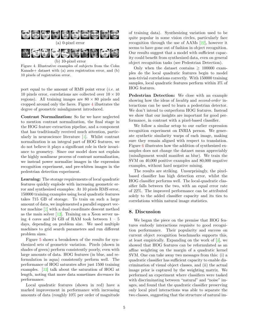
Figure 8. Visualisations of HOG and local quadratic classifiers on the INRIA person dataset. (a) A sample image fromthe set and its equivalent representation in (b) HOG space, and (e) local quadratic space. Lighter shades represent strongedges and correlations respectively. The positive training set mean in (c) HOG space and (f) local quadratic space. Positiveweights of the final classifiers in (d) HOG space and (g) local quadratic space. In both HOG and local quadratic space,the visualization of individual images shows significant extraneous informative, however the final classifiers are clearer.Interpreting the local quadratic classifier in (g) is difficult since the correlations cannot be interpreted as edges, however thedistribution of positive weights is similar to HOG, especially around the head and shoulders and between the legs.

ages can be exploited by local second-order statistics.Armed with only these principles, we set out to discoverwhether it was possible to learn an accurate classifier ina controlled expression recognition setting, and quan-tify how much data was required for varying amountsof geometric misalignment. Figure 5 illustrates thatwith enough synthesized data, a local quadratic clas-sifier can learn non-trivial pixel interactions necessaryfor predicting expressions. Finally, we applied these in-sights to a pedestrian detection task, and show in Fig-ure 7 that a significant fraction of HOG’s performancecan be attributed to preserving local second-order pix-els interactions, and not the image specific prior (i.e.edges) that it encodes. Inspecting the local quadraticclassifier visualization from Figure 8, one can see thatemphasis (strong positive support weights representedby lighter shades) is placed on the object boundaries -specifically around the head and shoulders and betweenthe legs - just as HOG does.

9. Conclusions

Linear SVMs trained on HOG features have per-vaded many visual perception tasks. We hypothesizedthat preserving local second-order interactions are atthe heart of their success. This is motivated by similarfindings within the human visual system. With thesesimple assumptions combined with large amounts oftraining data, it is possible to learn a classifier that per-forms well on a constrained expression recognition task,and within ballpark figures of a HOG-based classifiertailored specifically to an image prior on a pedestriandetection experiment. As the size of datasets contin-ues to grow, we will be able to rely less and less onprior assumptions, and instead let data drive the mod-els we use. Local second-order interactions are one ofthe simplest encoders of natural image statistics thatensure such models have the capacity to make informedpredictions.

7

References

[1] J. Bergstra, G. Desjardins, P. Lamblin, and Y. Ben-gio. Quadratic polynomials learn better image fea-tures. Technical report, Universite de Montreal, 2009.1

[2] S. Boyd. Distributed Optimization and StatisticalLearning via the Alternating Direction Method of Mul-tipliers. Foundations and Trends in Machine Learning,2010. 5

[3] H. Bristow and S. Lucey. V1-Inspired features inducea weighted margin in SVMs. European Conference onComputer Vision (ECCV), 2012. 1, 2, 5

[4] M. Carandini and D. J. Heeger. Normalization as acanonical neural computation. Nature reviews. Neuro-science, Jan. 2012. 5

[5] N. Dalal and B. Triggs. Histograms of oriented gradi-ents for human detection. Computer Vision and Pat-tern Recognition (CVPR), 2005. 1

[6] J. Daugman. Uncertainty Relation for Resolution inSpace, Spatial Frequency, and Orientation Optimizedby Two-Dimensional Visual Cortical Filters. OpticalSociety of America, Journal, A: Optics and Image Sci-ence, 1985. 2

[7] O. Deniz, G. Bueno, J. Salido, and F. De la Torre. Facerecognition using Histograms of Oriented Gradients.Pattern Recognition Letters, Sept. 2011. 1

[8] J. J. DiCarlo, D. Zoccolan, and N. C. Rust. How doesthe brain solve visual object recognition? Neuron,Mar. 2012. 1

[9] P. F. Felzenszwalb, R. B. Girshick, D. McAllester, andD. Ramanan. Object detection with discriminativelytrained part-based models. Pattern Analysis and Ma-chine Learning (PAMI), Sept. 2010. 1, 4

[10] B. Hariharan, J. Malik, and D. Ramanan. Discrim-inative decorrelation for clustering and classification.European Conference on Computer Vision (ECCV),2012. 2

[11] G. E. Hinton. Learning multiple layers of representa-tion. Trends in Cognitive Sciences, Oct. 2007. 4

[12] C.-J. Hsieh, K.-W. Chang, C.-J. Lin, S. S. Keerthi, andS. Sundararajan. A dual coordinate descent methodfor large-scale linear SVM. International Conferenceon Machine Learning (ICML), 2008. 5

[13] A. Hyvarinen and U. Koster. Complex cell pooling andthe statistics of natural images. Network, June 2007.1

[14] K. Kavukcuoglu, M. Ranzato, and R. Fergus. Learn-ing invariant features through topographic filter maps.Computer Vision and Pattern Recognition (CVPR),June 2009. 1

[15] K. Kavukcuoglu, P. Sermanet, Y.-l. Boureau, K. Gre-gor, M. Mathieu, and Y. LeCun. Learning con-volutional feature hierarchies for visual recognition.Advances in Neural Information Processing Systems(NIPS), 2010. 4

[16] A. Krizhevsky, I. Sutskever, and G. Hinton. Imagenetclassification with deep convolutional neural networks.

Advances in Neural Information Processing Systems(NIPS), 2012. 1

[17] H. Lee, R. Grosse, R. Ranganath, and A. Y. Ng. Con-volutional deep belief networks for scalable unsuper-vised learning of hierarchical representations. Interna-tional Conference on Machine Learning (ICML), 2009.4

[18] E. Simoncelli and B. Olshausen. Natural Image Statis-tics and Neural Representation. Annual Review ofNeuroscience, 2001. 2, 3

[19] O. Tuzel, F. Porikli, and P. Meer. Region covariance:A fast descriptor for detection and classification. Euro-pean Conference on Computer Vision (ECCV), 2006.2

[20] J. Xiao, J. Hays, and K. Ehinger. Sun database: Large-scale scene recognition from abbey to zoo. ComputerVision and Pattern Recognition (CVPR), 2010. 1

[21] Y. Yang and D. Ramanan. Articulated pose estimationwith flexible mixtures-of-parts. Computer Vision andPattern Recognition (CVPR), 2011. 1

[22] X. Zhang and Y. Gao. Face recognition across pose:A review. Pattern Recognition, Nov. 2009. 5

[23] X. Zhu, C. Vondrick, D. Ramanan, and C. Fowlkes.Do We Need More Training Data or Better Models forObject Detection? British Machine Vision Conference(BMVC), 2012. 5

8