Why credit money doesn’t have to crashAnd why it always does

Steve KeenUniversity of Western Sydney

Debunking Economicswww.debtdeflation.com/blogswww.debunkingeconomics.com

0 1 2 3 4 5 6 7 8 9 10 11 12 1325

20

15

10

5

0

5

10

15

20

25

Great Depressionincluding GovernmentGreat Recessionincluding Government

Debt-financed demand percent of aggregate demand

Years since peak rate of growth of debt (mid-1928 & Dec. 2007 resp.)

Per

cent

0

1870 1880 1890 1900 1910 1920 1930 1940 1950 1960 1970 1980 1990 2000 2010 20200

25

50

75

100

125

150

175

200

225

250

275

300

USAAustralia

Private debt to GDP ratios

Flow of Funds Table L1+Census Data; RBA Table D02

Yea

rs (

per

cent

of

GD

P)

The Great Moderation to The Great Recession• Everything was going SO well…

1975 1980 1985 1990 1995 2000 2005 2010 20155

0

5

10

15

UnemploymentInflation

The Great Moderation.. and Great Recession

Year

Per

cen

t

0

10

2008.5

Inflation & Unemploment Falling

Inflation & Unemploment Falling

Unem

plo

yment

Unem

plo

yment

Deflation

Deflation

What the hell happened?

• A debt bubble burst…

1920 1930 1940 1950 1960 1970 1980 1990 2000 2010 20200

20

40

60

80

100

120

140

160

180

200

220

240

260

280

300

320

USA Private Debt to GDP

Year

Per

cent

of

GD

P

175

2008.5

• Should that matter?

• Not according to conventional “neoclassical” economics…

Credit Money Myths• Neoclassical economics

– Debt not a problem because loans = savings• “Fisher’s idea was less influential in academic

circles, though, because of the counterargument that debt-deflation represented no more than a redistribution from one group (debtors) to another (creditors).” (Bernanke 2000, p. 24)

• Populist (& many non-neoclassical economists)– Inevitable problem because interest can’t be paid

• “The existence of monetary profits at the macroeconomic level has always been a conundrum … not only are firms unable to create profits, they also cannot raise sufficient funds to cover the payment of interest.” (Rochon 2005, p. 125)

Neoclassical myth: “Deposits create loans”

• Creation process:– Government creates Base Money (e.g., welfare

cheque)– Public puts BM in bank account– Bank keeps fraction (RR%: “reserve requirement”)– Lends rest: MB*(1-RR%)– Borrower deposits loan in another bank…– Iterative process generates BM/RR dollars

• Banks as– Passive amplifiers of government money creation– Mere intermediaries between savers & borrowers

• Loan transfers money from saver to borrower– Private Debt has minimal macroeconomic effect

• Only if borrower has higher propensity to spend

Reality: Endogenous money

• Banks create credit money “out of nothing”– “In the real world banks extend credit, creating

deposits in the process, and look for the reserves later” (Moore (1979, p. 539)—quoting Fed economist)

– “There is no evidence that … the monetary base … leads the cycle, although some economists still believe this monetary myth…, if anything, the monetary base lags the cycle slightly…

– The difference of M2-M1 leads the cycle by even more than M2 with the lead being about three quarters." (Kydland & Prescott 1990, p. 14)

• So credit money created “ab initio” by banks• And that doesn’t have to be a problem…

Model of credit money• Pure credit money system: bank issues own notes

– Like 19th century free banking in USA– No Central Bank

• Private bank formed by elite

• Notes “backed” by own wealth

• Lends to local businesses…• How did it work?• Stylised model with 5 accounts

• “Vault”—where bank stores its wealth• “Safe”—for spending, payment & receipt of

interest• “Loans”—ledger recording who owes bank how

much• “Firms”—deposit account for firms• “Workers”—deposit account for workers

• System starts with Notes (say $1 million) in Vault

19th century free banking: Stage 1 • $1 million in Vault, all other accounts zero…• Bank loans transfer notes from Vault to Firms• Bank records loans in its Loans ledger• Bank charges interest on loans• Firm pays interest which Bank deposits in its Safe• Bank records payment of interest on Loans ledger• Bank pays deposit interest to Firm• End result at this point:

• Over time, Vault emptied of Notes• Notes pass via Firms back to Banks’ Safe:

19th century free banking: Stage 1• Modelled using new software package QED

– “Quesnay Economic Dynamics”

QEDQED

19th century free banking: Stage 2• Closing the system: workers, factories & consumption• Firms pay wages to Workers• Bank pays workers interest on deposits• Workers and Bankers consume • End result at this point: System sustainable

• Firms make profits• Workers earn wages, Banks earn interest

Non-Neoclassical myth: “Interest can’t be repaid”• Common belief in Post-Keynesian economics &

populist views of money: No it isn’t– Interest can’t be repaid because loan less than

loan + interest; and firms can’t make monetary profits:• “The existence of monetary profits at the

macroeconomic level has always been a conundrum for theoreticians of the monetary circuit… not only are firms unable to create profits, they also cannot raise sufficient funds to cover the payment of interest. In other words, how can M become M`?” (Rochon 2005, p. 125)

– Wrong!– Confusion of stock (size of loan in $) with flow

(turnover of economic activity in $/year)

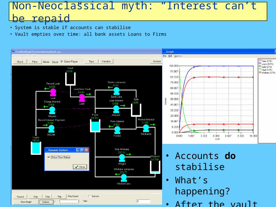
Non-Neoclassical myth: “Interest can’t be repaid”

• System is stable if accounts can stabilise• Vault empties over time: all bank assets Loans to Firms

• Accounts do stabilise

• What’s happening?• After the vault

empties…

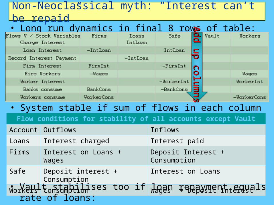
Non-Neoclassical myth: “Interest can’t be repaid”• Long run dynamics in final 8 rows of table:A

dd u

p co

lum

ns

Ad

d u

p co

lum

ns

• System stable if sum of flows in each column equal zeroFlow conditions for stability of all accounts except Vault

Account Outflows Inflows

Loans Interest charged Interest paid

Firms Interest on Loans + Wages Deposit Interest + Consumption

Safe Deposit interest + Consumption

Interest on Loans

Workers Consumption Wages + Deposit Interest• Vault stabilises too if loan repayment equals rate of loans:

19th century free banking: Stage 3• Firm repays loan which Bank puts back in Vault• Bank records repayment on Loan ledger

• Sustainable system• Bank assets now unlent Notes in Vault plus Loans to

Firms • Incomes for all classes• Wages $310.47 p.a.• Net Interest $3.72• Profit? 217.33 p.a.

(shown later)• Final step: new money

• In 19th century: notes

• In 20th century: credit

QEDQED

Money creation in pure credit economy• 19th century: add new notes to vault

Money creation in pure credit economy• 20th century: simultaneously issue loan and deposit

Money creation in pure credit economy• System not inherently unstable

– Firms can pay interest & make a profit– Debt can remain low & constant relative to GDP– Rising debt also necessary for expanding economy…

• “If income is to grow, the financial markets … must generate an aggregate demand that, aside from brief intervals, is ever rising.

• For real aggregate demand to be increasing, … it is necessary that current spending plans, summed over all sectors, be greater than current received income…

• It follows that over a period during which economic growth takes place, at least some sectors finance a part of their spending by emitting debt or selling assets.” (Minsky 1982, p. 6; emphasis added)

Money creation in pure credit economy

• Schumpeter on same issue: growing debt adds demand beyond that generated by sales of goods & services

• Debt essential for entrepreneurial function– Entrepreneur often has idea but no money– Needs purchasing power before has goods to sell– Gets purchasing power via loan from bank– Entrepreneurial demand thus not financed by “circular

flow of commodities” but by new bank credit– Since entrepreneurial activities essential feature of

growing economy, in real life “total credit must be greater than it could be if there were only fully covered credit. The credit structure projects not only beyond the existing gold basis, but also beyond the existing commodity basis.” (Schumpeter 1934, p. 101)

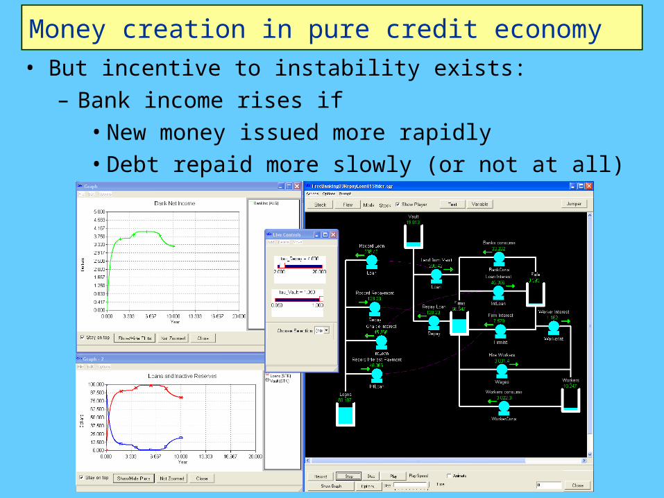
Money creation in pure credit economy• But incentive to instability exists:

– Bank income rises if• New money issued more rapidly• Debt repaid more slowly (or not at all)

Money creation in pure credit economy• Same result in modern banking; bank income rises if

– Bank reserves circulated more rapidly– Loans paid off more slowly– New loans created more rapidly

Money creation in our real economy• Banks have inherent bias to create debt• Borrowers control whether that bias is expressed• Income based borrowing—inherently limited• The “Solution”: lend to finance Ponzi Schemes

– Potential borrower expects asset price to rise– Borrows money to buy asset– Drives price of asset up– Rise entices other borrowers into market

• Positive feedback from leverage to prices causes asset price bubble

• Scheme “works until it fails”:– Rising debt-financed spending boosts economy– Requires acceleration in debt to continue forever…

The Facts on Debt

• 2 obvious US debt bubbles in last century

1920 1930 1940 1950 1960 1970 1980 1990 2000 2010 20200

20

40

60

80

100

120

140

160

180

200

220

240

260

280

300

320

USA Private Debt to GDP

Year

Per

cent

of

GD

P

175

2008.5

Debt and Aggregate Demand

• Conventional “exogenous money” economics– Debt has minor macroeconomic effects

• Redistributes money from lender to borrower• “Absent implausibly large differences in marginal

spending propensities among the groups, it was suggested, pure redistributions should have no significant macroeconomic effects.” (Bernanke 2000, p. 24)

• Realistic “endogenous money” economics– Increasing debt expands aggregate spending– Aggregate demand equals GDP plus change in

debt• Spent on all markets—goods + existing assets

– Volatile “change in Debt” component dominates economy as debt grows relative to income

0 1 2 3 4 5 6 7 8 9 10 11 12 13 14 15 16 17 18 19 20 214 10

6

6 106

8 106

1 107

1.2 107

1.4 107

1.6 107

1.8 107

2 107

GDP aloneGDP+Change in Debt+ Government

US Aggregate Demand GDP 1990-2010

Years since 1990

$ m

illio

n

18

Crisis by Crisis by de-de-

leveragingleveraging

Debt and Aggregate Demand• Crisis manifestation of deleveraging

But notice But notice recent recent

turnaroundturnaround

1975 1979 1983 1987 1991 1995 1999 2003 2007 2011 201536

30

24

18

12

6

0

6

12

18

24

30

36 0

11

10

9

8

7

6

5

4

3

2

1

0

Debt-financedInc. GovUnemployment

Correlation US debt-financed demand & unemployment

Year

Per

cent

cha

nge

p.a.

Per

cent

une

mpl

oyed

(in

vert

ed)

0

Debt and Aggregate Demand• Correlation with unemployment

Crisis by Crisis by de-de-

leveragingleveraging

But notice But notice recent recent

turnaroundturnaround

Acceleration in Debt & Change in Employment

• Since AD = GDP +D– AD = GDP +D– Changes in aggregate demand

• & hence changes in employment– Correlated not with change in debt (D)

• But with acceleration/deceleration in debt (D)• Defining “credit impulse” (Biggs, Meyer & Pick) as

ChangeI nChangeI nDebtGDP

• Empirically, credit—ignored by neoclassical economics—is the key driver of the economy...

1955 1960 1965 1970 1975 1980 1985 1990 1995 2000 2005 2010 201530

25

20

15

10

5

0

5

10

Acceleration of private debtChange in Private Employment

Acceleration of private debt & change in employment, USA

Year

Per

cent

p.a

.

0

2008

Change in Debt & Change in Employment

• Correlation with change in employment

USA stalled crisis by USA stalled crisis by slowdown in slowdown in deleveragingdeleveraging

Crisis Crisis beginsbegins

Change in Debt & Change in Employment

• Summing up: Credit drives the economy• Acceleration in debt precedes change in GDP

20 10 0 10 20 300.2

0

0.2

0.4

0.6

0.8

EmploymentGDP

Credit Impulse Correlations in the USA

Lag in months

Cor

rela

tion

0 • Doesn’t have to drive it “over the cliff”

• But always does• Why?• The temptation

of Ponzi Finance• Putting it all

together...

Finance and Economic Breakdown

• Economy is– Inherently cyclical

• Waves of innovation/destruction (Schumpeter)• Struggles over income distribution (Marx, Goodwin)• Complex & aperiodic (Lorenz, Mandelbrot,

Prigogine)– Inherently monetary

• Moore, Graziani– Inherently afflicted by uncertainty

• Keynes (not IS-LM!)• Given nature of capital assets

– Banks’ desire to create debt leads to financial crises• The Financial Instability Hypothesis: Minsky

Minsky’s “Financial Instability Hypothesis”

• Economy in historical time– Both ignored by conventional “neoclassical”

economics)• Debt-induced recession in recent past• Firms and banks conservative re debt/equity, assets• Only conservative projects are funded

– Recovery means most projects succeed• Firms and banks revise risk premiums

– Accepted debt/equity ratio rises– Assets revalued upwards…

• “Stability is destabilising”– Period of tranquility causes expectations to rise…

• Self-fulfilling expectations– Decline in risk aversion causes increase in investment– Investment expansion causes economy to grow faster

The Euphoric Economy

• Asset prices rise: speculation on assets profitable• Increased willingness to lend increases money supply

– Money supply endogenous , not under RBA control• Riskier investments enabled, asset speculation

rises• The emergence of “Ponzi” (Bond, Skase…) financiers

– Cash flow less than debt servicing costs– Profit by selling assets on rising market– Interest-rate insensitive demand for finance

• Rising debt levels & interest rates lead to crisis– Rising rates make conservative projects speculative– Non-Ponzi investors sell assets to service debts– Entry of new sellers floods asset markets– Rising trend of asset prices falters or reverses

The Assets Boom and Bust

• Ponzi financiers go bankrupt:– Can no longer sell assets for a profit– Debt servicing on assets far exceeds cash flows

• Asset prices collapse, increasing debt/equity ratios• Endogenous expansion of money supply reverses• Investment evaporates; economic growth slows• Economy enters a debt-induced recession

– Back where we started...• Process repeats once debt levels fall

– But starts from higher debt to GDP level• Eventually final crisis where debt burden overwhelms

economy

Modelling Minsky

• Modelled by– Introducing nonlinear functions

• Capitalist desire to invest• Debt repayment rate• Money relending rate

– Endogenous money creation via “line of credit”• Firm investment desire funded by increased

deposit• Simultaneous increase in debt

– Modelling production & price formation• Also growth in population & labor productivity

Modelling Minsky: Financial side• New Godley Table

““Line of Line of credit”: credit”:

money & money & debt created debt created

at same at same timetime

• Exponential functions for expectations under uncertainty:• Given uncertain future, investors assume that “the

present is a much more serviceable guide to the future than a candid examination of past experience would show it to have been hitherto” (Keynes 1936, p. 214)

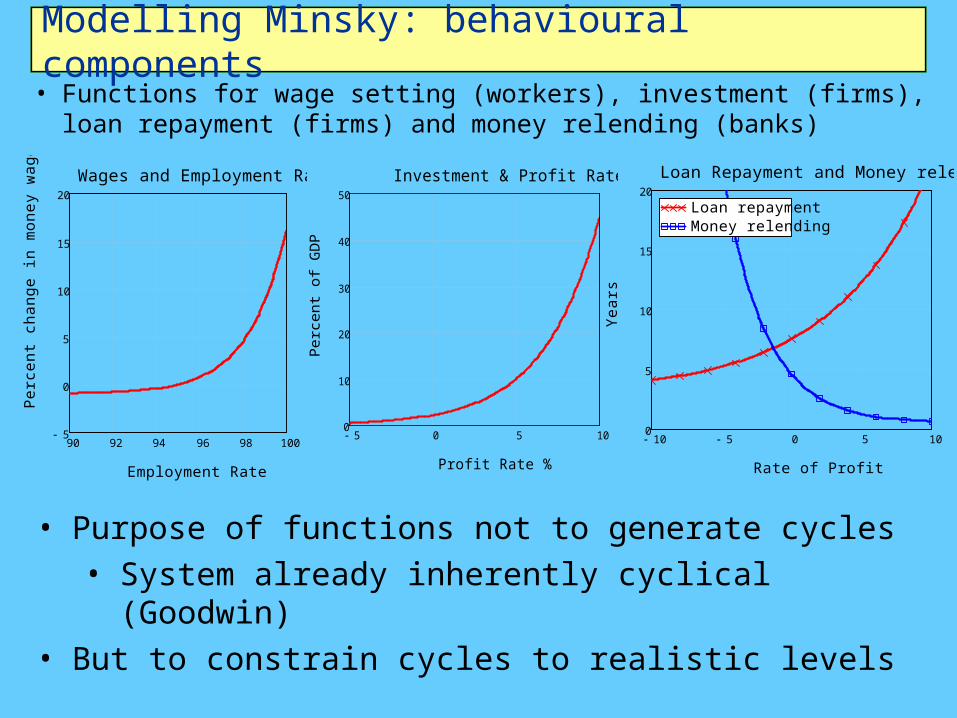
Modelling Minsky: behavioural components• Functions for wage setting (workers), investment (firms),

loan repayment (firms) and money relending (banks)

90 92 94 96 98 1005

0

5

10

15

20

Wages and Employment Rate

Employment Rate

Per

cent

cha

nge

in m

oney

wag

es

5 0 5 100

10

20

30

40

50

Investment & Profit Rate

Profit Rate %

Perc

ent o

f GD

P

10 5 0 5 100

5

10

15

20

Loan repaymentMoney relending

Loan Repayment and Money relending

Rate of Profit

Yea

rs

• Purpose of functions not to generate cycles• System already inherently cyclical (Goodwin)

• But to constrain cycles to realistic levels

Modelling Minsky: Production Relations

• Capital K determines output Y via the accelerator:

Y/

lr1

Labour Productivitya

L

• Y determines employment L via productivity a:

• L determines employment rate l via population N:

• l determines rate of change of wages w via Phillips Curve

• Integral of w determines W (given initial value)

• Y-W determines profits P and thus Investment I…dw/dt 1/S

Integrator

w++

1Initial Wage

*L

W

WY +

-Pi I dK/dt

• Closes the loop:

1Initial Capital +

+1/SIntegrator

dK/dt

K 1/3Accelerator

Y

L/

lr100

PopulationN

l

PhillipsCurve dw/dt+- *

10WageResponse

.96"NAIRU"

• (Linear Phillips curve for (Linear Phillips curve for now)now)

Modelling Minsky: Inherent cycles

• Model generates cycles (but no growth since no population growth or technical change yet)…:

K 1/3Accelerator

Y

/lr1

Labour Productivitya

L

/lr

1Population

Nl

PhillipsCurve dw/dt

1/SIntegrator

w++

1Initial Wage *

LW

Y +-

Pi I dK/dt

3Initial Capital +

+1/SIntegrator

+- *10

WageResponse

.96"NAIRU"

Goodwin's cyclical growth model

Time (Years)0 2 4 6 8 10

.50

.75

1.00

1.25

1.50Employment

Wages

Goodwin's cyclical growth model

Employment.9 .95 1 1.05

Wa

ge

s

.7

.8

.9

1.0

1.1

1.2

1.3

Goodwin01B.vsm

• Cycles caused by essential nonlinearity:

• Wage rate times employment

• Behavioural nonlinearities not needed for cycles;

• Instead, restrain values to realistic levels

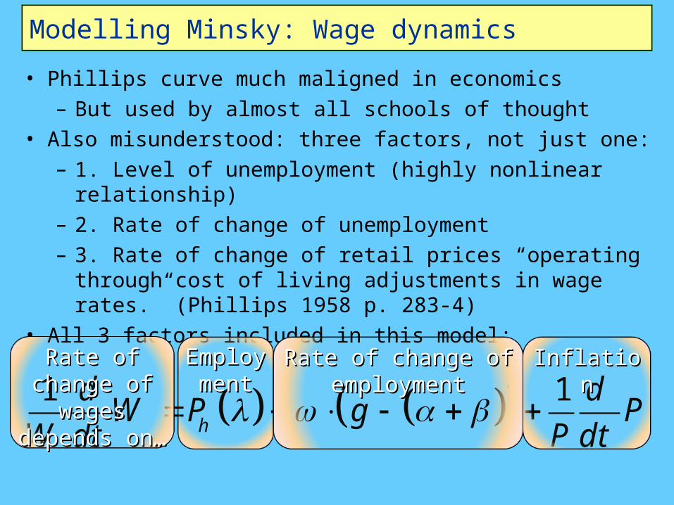
Modelling Minsky: Wage dynamics

• Phillips curve much maligned in economics– But used by almost all schools of thought

• Also misunderstood: three factors, not just one:– 1. Level of unemployment (highly nonlinear

relationship)– 2. Rate of change of unemployment– 3. Rate of change of retail prices “operating through

cost of living adjustments in wage rates.” (Phillips 1958 p. 283-4)

• All 3 factors included in this model:

1 1

h

d dW P g P

W dt P dt

EmployEmploymentment

Rate of change of Rate of change of employmentemployment

InflationInflationRate of Rate of change of change of

wages wages depends depends

on…on…

Modelling Minsky: Price dynamics

• Physical Output (Q) = Labor times L labor productivity a• Labor = Money flow of wages divided by money wage W• Flow of wages = worker share of output during turnover

period S (time from outlays to receipts)

• Money Demand = Annual flow of wages plus profits

– = Money in Firms divided by turnover S .

• Physical Demand = Money demand divided by Price level• In equilibrium, flow of physical supply = physical demand

1 1

e eD D

e eS S e

F FsQ a D

W P

• Solving for equilibrium price:

1

1e

WP

as

• As a dynamic process:

1 1

1P

d WP P

dt as

Convergence over timeConvergence over time

PhysicaPhysical l

demandemandd

Physical Physical supplysupply

Modelling Minsky: The full system

•In

scary

equatio

ns…

Financial Sector

tBC t( )d

d

FL t( )

RL r t( ) BC t( )

LC r t( ) BC 0( ) BC0

tBPL t( )d

drL FL t( ) rD FD t( ) rD WD t( )

BPL t( )

B BPL 0( ) BPL0

tFL t( )d

d

BC t( )

LC r t( ) FL t( )

RL r t( ) PC t( ) Yr t( ) Inv r t( ) FL 0( ) FL0

tFD t( )d

drD FD t( ) rL FL t( )

BC t( )

LC r t( ) FL t( )

RL r t( ) BPL t( )

B

WD t( )

W PC t( ) Yr t( ) Inv r t( )

W t( ) Yr t( )

a t( ) FD 0( ) FD0

tWD t( )d

drD WD t( )

WD t( )

W

W t( ) Yr t( )

a t( ) WD 0( ) WD0

Physical output, labour and price systems

Level of output Yr 0( ) Yr0Yr t( )Kr t( )

v

Employment L t( )Yr t( )

a t( )L 0( ) L0

Rate of Profit r t( )PC t( ) Yr t( ) W t( ) L t( ) rL FL t( ) rD FD t( )

v PC t( ) Yr t( ) r 0( ) r0

Rate of employmentt t( )d

d t( ) g t( ) ( )[ ] 0( ) 0

Rate of real economic growth g t( )Inv r t( )

v g 0( ) g0

tW t( )d

dW t( )( ) Ph t( )( ) g t( ) ( )[ ][ ]

1Pc

1W t( )

a t( ) 1 s( ) PC t( )

Rate of change of wages W 0( ) W0

Rate of change of prices PC 0( ) PC0tPC t( )d

d

1Pc

PC t( )W t( )

a t( ) 1 s( )

Rate of change of capital stocktKr t( )d

dKr t( ) g t( ) Kr 0( ) Kr0

Rates of growth of population and productivityta t( )d

d a t( )

tN t( )d

d N t( ) N 0( ) N0 a 0( ) a0

Modelling Minsky: The full system

•In

less sca

ry Q

ED

form

at:

QEDQED

Modelling Minsky: The outcome• Model generates Great Moderation & Great Recession

– Not yet calibrated on data yet qualitatively similar…

70 72 74 76 78 80 82 84 86 88 90 92 94 96 98 100 102 104 106 108 1102

0

2

4

6

8

10

12

14

16

InflationUnemploymentU-6 Measure

US Inflation and Unemployment since 1970

Year

Per

cent

70 72 74 76 78 80 82 84 86 88 90 92 94 96 98 100 102 104 106 108 1102

0

2

4

6

8

10

12

14

16

InflationUnemploymentU-6 Measure

US Inflation and Unemployment since 1970

Year

Per

cent

0 10 20 30 40 50 60 70 80 90 100 1105

0

5

10

15

InflationUnemployment

Great Moderation to Great Recession

Year

Per

cen

t p.a

.

0

Modelling Minsky: The outcome

• The full picture from QED

Modelling Minsky: The outcome

• The full picture from QED

Modelling Minsky: The insights

• Private debt causes both boom and crisis• Workers pay for debt through reduced share of income:

0 20 40 6010

0

10

20

30

40

50

60

70

80

90

100

110

WorkersCapitalistsBankers

Income Distribution

Year

Per

cent

of

GD

P

• Reduced volatility with rising debt a sign of• Not increased

stability (“The Great Moderation”—Bernanke 2004)

• But “Calm before the storm” (Keen 1995)

0 1 2 3 4 5 6 7 8 9 10 11 12 1325

20

15

10

5

0

5

10

15

20

25

Great Depressionincluding GovernmentGreat Recessionincluding Government

Debt-financed demand percent of aggregate demand

Years since peak rate of growth of debt (mid-1928 & Dec. 2007 resp.)

Per

cent

0

How does “Now” compare to “Then”?

• Debt-financed proportion of aggregate demand:Debt

GDP Debt

Where to from here?

• 3 factors determine debt impact on economy– Level (relative to GDP)

• Like distance between start and destination• How long before journey is over

– Rate of change• Like speed of travel to destination• Affects aggregate demand

– Rate of change of rate of change• Like acceleration/deceleration• Whether you’re getting there more quickly or not• Affects rate of change of aggregate demand

– Are things improving or getting worse right now?

Where to from here?: Level• It’s a long way from the top if you’ve sold your soul...

1920 1930 1940 1950 1960 1970 1980 1990 2000 2010 20200

20

40

60

80

100

120

140

160

180

200

220

240

260

280

300

320

USA Private Debt to GDP

Year

Per

cent

of

GD

P

75

175

2009.5• Almost 100% of

GDP reduction to get to pre-Great Depression level• Speculative

debt still present

• 200% to get back to 50s level• Only

productive debt

• Decade with aggregate demand below GDP

The NBER thinks The NBER thinks the recession the recession ended here!ended here!

Where to from here?: Rate of change

• Deleveraging impact equivalent to Great Depression level

1980 1982 1984 1986 1988 1990 1992 1994 1996 1998 2000 2002 2004 2006 2008 2010 201230

25

20

15

10

5

0

5

10

15

20

25

30 0

5

0

Debt-financed demandUnemployment (inverted)

Velocity of debt & unemployment

Year

Perc

en

t o

f ag

gre

gate

dem

and

U-3

measu

re o

f un

em

plo

ym

en

t

0

2009.5

• Debt reducing at Great Depression rate• Levelling out implies sustained slump

• “Turning Japanese”

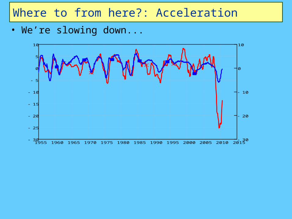
Where to from here?: Acceleration• We’re slowing down...

1955 1960 1965 1970 1975 1980 1985 1990 1995 2000 2005 2010 201530

25

20

15

10

5

0

5

10

30

20

10

0

10

Acceleration of debtRate of change of employment

Acceleration of debt & change in employment

Year

Rate

of

ch

an

ge o

f n

ew

deb

t p.a

.

Rate

of

ch

an

ge o

f p

riv

ate

em

plo

ym

en

t p

.a.

0

2009.5

• Less scary than accelerating fall (rising on quarterly data)

• But still not enough to increase employment• Susceptible to future acceleration in fall

• Much of rise driven by return to Ponzi investing

The acceleration effect The acceleration effect might be why the NBER might be why the NBER thinks the recession thinks the recession ended here!ended here!

Where to from here?

• 2 most persistent debt metrics remain negative– Level of debt to GDP– Rate of change

• Most volatile currently positive– Deceleration of deleveraging

has boosted economy• Learning complicated

dynamics of debt the hard way• History implies crisis has many

years to run…