Embed Size (px)
Citation preview

Why Are Indian Children Shorter Than African
Children?∗
Seema Jayachandran
Northwestern University
Rohini Pande
Harvard University
July 27, 2013
Abstract
Height-for-age among children is lower in India than in Sub-Saharan Africa. This
presents a puzzle since India is richer than the average African country and fares
better on most other development indicators including infant mortality. Using data
from African and Indian Demographic and Health Surveys, we document three facts.
First, among firstborns, Indians are actually taller than Africans; the Indian height
disadvantage appears with the second child and increases with birth order. Second,
investments in successive pregnancies and higher birth order children decline faster
in India than Africa. Third, the India-Africa birth order gradient in child height
appears to vary with sibling gender. These three facts suggest that parental preferences
regarding higher birth order children, driven in part by cultural norms of eldest son
preference, underlie much of India’s child stunting.
∗We thank Suanna Oh and Alexander Persaud for excellent research assistance, and Jere
Behrman, Angus Deaton, Jean Dreze, Erica Field, Dominic Leggett, Nachiket Mor, Debraj Ray,
Alessandro Tarozzi and several seminar and conference participants for comments. Contact infor-
mation: Jayachandran: [email protected]; Pande: [email protected].

1 Introduction
Despite India’s strong growth performance in recent years, a striking proportion of
Indian children continue to fall short of their height potential. Over 40 percent of Indian
children age five years and younger are classified as stunted (IIPS, 2010), and Figure 1 shows
that Indian (and more broadly South Asian) children are shorter than those born in other
low-income regions such as Sub-Saharan Africa. The India-Africa child height disparity
stands in sharp contrast to India’s relatively better performance on most other health and
socioeconomic indicators ranging from infant and maternal mortality and life expectancy
to food security, poverty incidence and educational attainment (Gwatkin et al., 2007), and
suggests potential limits on the future prosperity on young Indians.1
The biological literature on the determinants of child height identifies two distinct po-
tential explanations for the India-Africa gap: genetic and environmental.2 In this paper, we
use 27 Sub-Saharan African and one Indian Demographic and Health Survey (DHS) con-
ducted since 2004 to demonstrate the importance of parental preferences within the class of
environmental explanations. We find a much greater height drop-off for later-born children
in India than in Africa: Height-for-age is actually higher in India than in Africa for firstborn
children. The Indian height disadvantage materializes for second-born children and increases
for third and higher order births, at which point Indian children have a mean height-for-age
lower than that of African children by 0.35 standard deviations of the worldwide distribution.
We see the same pattern – a much steeper birth order gradient in child height in India than
in Africa – when the estimation is limited to between-sibling variation. Thus, birth order is
not just proxying for family background differences between smaller and larger families.
This birth order pattern suggests that the prevalence of malnutrition in India is not an
artefact of using child height to measure malnutrition rates (Panagariya, 2013). Genotypes
do not vary with birth order, so a simple genetic predisposition to be short likely would
not generate the very significant birth order effects we find. In addition, the birth order
1The Indian Prime Minister Manmohan Singh has called the problem “a national shame,” stating that,“We cannot hope for a healthy future for our country with a large number of malnourished children,” (Sinha,2012). In the academic literature, early-life malnutrition, with stunting as a marker, has been associated withimpaired immunocompetence (Falkner and Tanner, 1989), poor cognitive skills and education attainment(Glewwe and Miguel, 2007) and overall functional impairment (Barker and Osmond, 1986; Barker et al.,1993) and has been linked to detrimental effects on long-term economic status (Strauss and Thomas, 1998;Case and Paxson, 2008).
2Adult height is largely determined in the first few years of life (Tanner et al., 1956).
1
pattern does not appear to reflect differential infant survival or initial maternal health. For
differential mortality selection to explain the birth order effect, we would need India’s infant
survival to be especially high for later-born children since this is where the Indian height
disadvantage is largest. But in fact the opposite pattern is seen: the infant survival rate in
India is particularly high at low birth order. Regarding initial maternal health, it is possible
that Indian women are unhealthier than African women at the start of childbearing and,
therefore, predisposed to having smaller babies.3 This environmental explanation posits
that the die is cast during the mother’s childhood and adolescence. However, the impact
of mother’s height, a summary measure of a woman’s health inputs before adulthood, on
child height does not vary much with birth order. Thus, it appears that the birth order
gradient in child height reflects contemporaneous choices by households rather than the past
environment the mother faced before entering her childbearing years.
The within-family patterns in child height also cast doubt on simply access to services
as the explanation, since access typically does not vary substantially with the child’s birth
order, and instead point to take-up of services. In the remainder of the paper we provide
evidence that variation in stunting within households reflects parental preferences and their
decisions concerning when services and household resources are utilized. We explore two
classes of explanations for the strong birth order gradient in India: household resource
constraints and cultural norms that influence preferences toward children of different birth
order. The evidence points against resource constraints and in favor of parental preferences
as the underlying explanation. In particular, eldest son preference seems to help explain
Indian families’ relatively higher investment in earlier-born children.
Regarding household resources as a potential explanation, if families are liquidity con-
strained, then even with identical preferences over birth order in India and Africa, the child
height patterns could emerge if the time profile of income declines more steeply (or in-
creases less steeply) for families in India. Indian families might simply not have the financial
resources to spend on later-born children. A related hypothesis is that there are smaller
economies of scale in care-giving in India, so African families effectively have more resources
to spend on later born children. Two pieces of evidence militate against these explanations.
First, we analyze food consumption patterns across Indian and African mothers and find a
3This maternal health channel is an important contributor to the “gradual catch-up” hypothesis (Deatonand Dreze, 2009), according to which it takes time for a historically malnourished population to meet theirgenetic potential, even when their nutrition improves.
2

relatively greater decline in food consumption among Indian mothers as family size increases.
However, this decline is concentrated among pregnant women, suggesting an explicit decline
in investments in pregnant women rather than a generalized decrease in financial resources
(or even treatment of women). Second, comparing the food consumption of Indian women
and their husbands, we find that the pattern of food consumption declining as the family
size increases is concentrated only among pregnant women and not their husbands. Thus,
it appears that Indian households disinvest relatively more in women across successive preg-
nancies. The fact that the disinvestment is accentuated during pregnancy is suggestive of
an explicit preference over child health, but it could be the case that child health is an unin-
tended consequence. Women’s food consumption, body mass index, and hemoglobin levels
decline more with successive pregnancies in India; these effects would be detrimental to fetal
and child health, whether or not the family is aware of this implication.
However, further evidence points to a more conscious preference over children’s health.
Several arguably time-intensive prenatal health inputs such as prenatal checkups, maternal
iron supplementation, and childbirth at a health facility exhibit a stronger drop-off with
birth order in India than Africa. Moreover, postnatal inputs such as child vaccinations and
postnatal checkups, which are not indirect inputs to child health made via maternal health,
also sharply decline with birth order in India. In addition, later in life, we see a steep birth
order drop-off in parents’ investment in their children’s education in India, which is also
consistent with Indians having a relatively weaker preference for higher birth order children.
We next ask whether the stronger preference for earlier born children in India may, at
least partially, reflect a cultural norm of eldest son preference. A large literature documents
how higher economic returns associated with sons combined with the kinship rules of Hin-
duism (Dyson and Moore, 1983) and the Hindu requirement that only a male heir can light
the funeral pyre (Arnold et al., 1998) implies that son preference is strongest for the firstborn
son (Gupta, 1987).
Indeed, we find suggestive evidence that the birth order gradient in height depends on
the sex of older siblings. The small stature of later-born boys in India is larger if they have an
older brother; once the family has its eldest son, it seems to disinvest in subsequent children.
Moreover, this “advantage” of having only older sisters is not seen for girls, presumably
because in these cases the family expects to have another child to try for a son, so holds back
on spending on the current daughter. Thus, eldest son preference appears to generate a birth
3

order gradient in child health in India through high investments in utero for the potential
eldest son in the family (which disfavors later-born girls and boys), through fertility stopping
rules (which disfavor later-born girls), and potentially through exhaustion of resources on
the eldest son (which disfavors later-born girls and boys).
This paper makes several contributions. First, we add to the literature on the causes
of India’s high rate of child malnutrition. One approach has been to ask whether the rate
is really as high as Indians’ short stature would suggest, testing for the potential role of
genetics by examining whether wealthy and well fed Indian children are short by international
standards. The findings are mixed (Bhandari et al., 2002; Tarozzi, 2008; Panagariya, 2013).
Another approach is to examine the height of Indian children who migrate to rich countries,
with most authors finding that the gap between the Indian-born children and worldwide
norms narrows but does not close (Tarozzi, 2008; Proos, 2009). We take a different approach
of examining within-family patterns. Our results give support to the environment side of the
the genes-versus-environment debate, and therefore are complementary to papers such as
Spears (2013), which points to open defecation as an environmental explanation for India’s
high rate of stunting.4 However, we offer a quite different type of environmental explanation:
parental choices regarding resource allocation across children. Our work is related to Mishra,
Roy, and Retherford (2004) who also examine intrahousehold patterns, using earlier rounds
of the Indian DHS to show that stunting in India varies with the gender composition of
siblings. Also related is Coffey, Spears, and Khera (2013) who compare first cousins living
in the same Indian joint household and show that children born to the younger brother in
the household do worse, potentially due to the mother facing greater discrimination.
Second, we add to the growing literature on the ramifications – including unintended
ones – of son preference in India (Sen, 1990; Clark, 2000; Jensen, 2003; Jayachandran and
Kuziemko, 2011). In this case, son preference causes inequality in health inputs and outcomes
even among sisters. Third, we contribute to a much broader literature on inequality in
parental allocations among children (Rosenzweig and Schultz, 1982; Behrman, 1988; Garg
and Morduch, 1998). Finally, we add to a literature on the effects of birth order, which
4Spears (2013) shows that the high rate of open defecation in India helps explain the high rate of childstunting. There are reasons to think this channel could contribute to the birth order gradient, for exampleif older siblings expose younger siblings to disease or if the childcare of higher birth order children is lessvigilant. However, empirically, open defecation has smaller effects or no differential effects on height forhigher birth order children.
4

has documented gradients in outcomes as varied as IQ, schooling, height, and personality
(Behrman and Taubman, 1986; Sulloway, 1996; Black, Devereux, and Salvanes, 2007; Savage,
Derraik, Miles, et al., 2013). Our contribution to this literature is to document the strong
birth order effects in India and to demonstrate how birth order effects account for the entire
height gap between Indian and African children.
The remainder of the paper is organized as follows. Section 2 describes the data and
presents descriptive statistics for the sample. Section 3 presents evidence on the birth order
gradient in the Indian height disadvantage, and Section 4 examines potential explanations
for this gradient. Section 5 concludes.
2 Data and descriptive statistics
Our analysis uses data from Indian and African household surveys which we describe
below. We then use these data to provide a simple descriptive analysis of the India-Africa
height gap.
2.1 Demographic and Health Surveys
The data used for analysis come from Demographic and Health Surveys (DHS) for Sub-
Saharan African countries plus India’s National Family Health Survey (NFHS), which uses
the Demographic and Health Survey questionnaire (throughout we refer to this set of surveys
as the DHS). For India, we focus on the most recent round from 2005-6 (NFHS-3). As a
comparison group, we use all 27 Sub-Saharan African surveys (which represent 25 countries)
that collected child anthropometric data and were conducted between 2004 and 2010 (to
ensure a comparable time period to NFHS-3).
The surveys sample and interview mothers who are 15 to 49 years old at the time of
survey. Child height and weight are collected for respondents’ children who were under five
years of age at the time of the interview.5 Our sample comprises the 174,157 children with
non-missing anthropometric data. Appendix Table 1 provides summary statistics for the
Indian and African samples. The average age of the children in the sample is 30.1 months
in India and 28.1 months in Africa. The mother’s average age at birth is 24.8 years in India
and 27.0 years in Africa. African women have had more children (3.9) than their Indian
5The DHS nominally collects anthropometric data for children less than 60 months old, but many childrenwho are in their 60th month of life are missing anthropometric data. Hence we limit the sample to childrenwho are 59 months old or younger, or have not completed 59 months of life.
5

counterparts (2.7).
A key variable of interest is birth order. The DHS records the date of birth for all
children ever born, and we define birth order based on all children ever born, currently alive
or deceased.
To make height comparisons across children of different age and gender, we combine
anthropometric data on the child’s height with information on the date of measurement and
the child’s date of birth to create the child’s height-for-age z-score based on World Health
Organization (WHO) guidelines. For each combination of gender and age in months, the
WHO provides the distribution of these measures for a reference population of children from
Brazil, Ghana, India, Norway, Oman and the United States. A z-score of 0 is the median
of the reference population. A z-score of -1 indicates that the child is 1 standard deviation
below the reference-population median for his or her gender and age. A height-for-age z-score
of -2 is the cutoff for being considered stunted. The average height-for-age z-score in India
and Africa are -1.58 and -1.44, respectively. We similarly use the child’s weight to calculate
weight-for-age and weight-for-height z-scores. The average weight-for-age z-score in India
and Africa are -1.55 and -0.87.
The DHS also collects anthropometric data for the mother, including her height, weight,
and hemoglobin levels. We also use data collected on health-related behaviors during preg-
nancy including the number of prenatal care visits a mother had during the pregnancy and
whether she took an iron supplementation during the pregnancy, as well as her food con-
sumption patterns, namely how often she ate particular kinds of foods such as fruits or meat
or eggs. In general, India performs better on the prenatal inputs and worse on the measures
of pregnant women’s health. For example, 68 percent of the time, pregnant women in India
took iron supplements, compared to 62 percent in Africa, while the average BMI of pregnant
women is 21.1 in India and 23.0 in Africa.
We examine data on health inputs and outcomes for young children including incidence
of exclusive breastfeeding, whether the child had diarrhea in the past two weeks, whether
he or she received a postnatal checkup within the first two months, whether he or she was
given iron supplementation, and the total number of vaccinations.6 Vaccination rates are
higher on average in India, while child iron supplementation is more common in Africa. The
6We restrict attention to vaccinations for which the DHS collects data (BCG, three doses of DPT, fourdoses of polio, and measles); this analysis is restricted to children age one year and older who should havecompleted their course of vaccinations.
6
incidence of child diarrhea, as reported by the mother, is considerably higher in Africa than
India. We also consider domestic violence as an outcome, specifically whether the woman
has been the victim of any physical violence by the husband.7 The rate is 28 percent in India
and 26 percent in Africa. Appendix Table 2 shows the correlation between child height and
these several variables.
Some of these variables, such as anemia or food consumption or domestic violence, are
measured at the mother level while others are child-level variables. In addition, some of the
child-level variables are asked retrospectively of all children age three years and younger or
five years and younger, while most are asked only of the most recent birth. For this reason,
as well as due to missing values, the sample analyzing these outcomes is often smaller than
the full sample analyzing height, and we will not be able to estimate mother fixed effects
models with most of these variables.
We also examine infant mortality and children’s schooling as outcomes. For infant
mortality, the sample includes all alive or deceased children, excluding those whose date of
birth is less than one year before the survey date; the outcome of whether the child died
before age one is not fully determined until he or she reaches (or could have reached) age
one year. The infant mortality sample consists of children age 13 to 59 months comprises
199,696 children. The rate is 5 percent in India and 7 percent in Africa. For children’s years
of education, we use a sample of children age 7 to 17.8 Average years of schooling is 4.5
years in India and 2.4 years in Africa.
2.2 Covariate analysis
To set the stage for our analysis, we describe how some of the most commonly discussed
determinants of the Indian height disadvantage influence the India-Africa child height-for-
age (HFA) gap. We estimate for child i born to mother m in country c a regression of the
form
HFAimc = αIc + βYmc + γCimc + δGimc + φXmc + εimc. (1)
7Ackerson and Subramanian (2008) use Indian NFHS data to show a correlation between spousal violenceand child malnutrition. They posit two channels – first, that spousal violence is often accompanied bywithholding food consumption from the mother and second, violence increases maternal stress.
8Age 7 is the typical school-entry age, and we exclude children over age 17 years since those living athome will be a non-random sample.
7

The regression includes dummy variables for the survey year Ymc, the child’s age in months
Cimc, and the child’s gender Gimc, to adjust for any sampling differences between India and
Africa. In all cases, standard errors are clustered at the mother level. The coefficient α on
the India dummy Ic is an estimate of the India-Africa gap. Column (1) of Appendix Table
3 reports this gap when no other covariates are included: The gap is -0.14, measured in
standard deviations of the worldwide distribution, and significant at the 1 percent level.9
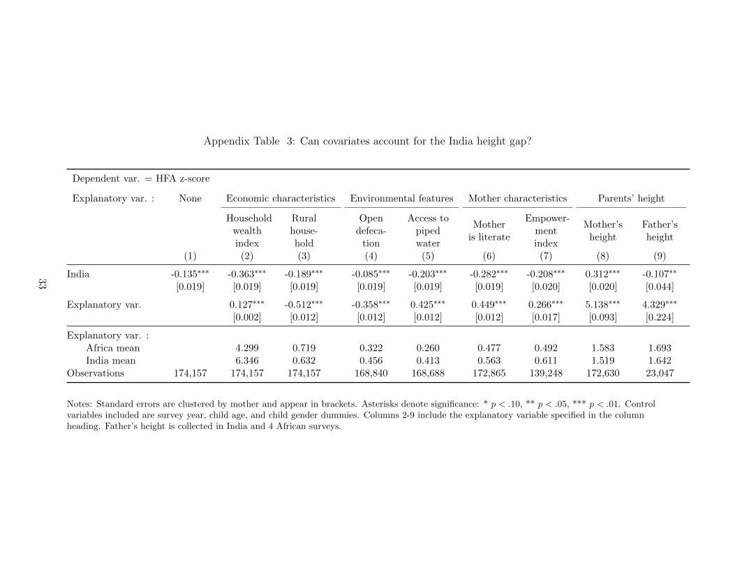
We control for several factors that have been proposed as explanations for Indian mal-
nutrition and examine whether these covariates “knock out” the India coefficient. The
remaining columns of Appendix Table 3 report these regressions where we include different
household-level covariates (Xmc). While we do not intend to make causal claims from these
correlations, this exercise suggests little prima facie support for most posited explanations.
We first examine how the India-Africa gap changes after controlling for various envi-
ronmental factors. Columns (2) to (7) of Appendix Table 3 considers three widely discussed
categories of environmental factors: household economic characteristics, access to clean wa-
ter and sanitation, and female empowerment. Our measures of household-level economic
measures are a household asset index and a dummy for rural. Columns (2) and (3) show
that in both cases, India is more developed than Africa, and controlling for these makes the
India coefficient larger in magnitude. These patterns echo what was seen in Figure 1 that
overall economic development as measured by GDP is not the explanation; GDP is higher
in India than the African countries in the sample.
Turning to access to water and sanitation, controlling for piped water makes the India
gap larger (column 4). In contrast, open defecation is more common in India than in Africa
and is negatively correlated with child height, so controlling for it reduces the India gap
by one third (column 5). Of the environmental factors studied, open defecation seems like
the most likely to contribute to the India-Africa height gap, consistent with the findings of
Spears (2013). Nonetheless, over two thirds of the gap remains unexplained after adjusting
for open defecation rates.
Many papers document a greater willingness by mothers, relative to fathers, to devote
resources towards children (Thomas, 1990). However, on observed measures of empowerment
such as female literacy and women’s decision-making, women in India fare better than those
in Africa, so controlling for them makes the India gap larger. To summarize, for most
9The raw India-Africa gap is also -0.14 and significant at the 1 percent level with no covariates included.
8

environmental factors proposed as explanations for the India height gap, India does better
than Africa on observable measures. Furthermore, the correlation between these factors
and HFA is generally too small to explain the India height gap. Thus pursuing standard
environmental explanations for the gap arguably heightens the puzzle of stunting in India
more than it solves it.
We next turn to examining if this simple accounting approach provides more support
for a genetic explanation. Columns (8) and (9) control for parental height, which should
capture the genetic component of child height. The patterns are quite striking. Mother’s
height is a strong predictor of child height, and controlling for it reverses the India-Africa
gap in child height. However, just as strikingly, controlling for father’s height only reduces
the gap by 20 percent.10 This pattern indicates that maternal height should not be inter-
preted as measuring purely genetics; the asymmetry with father’s height suggests that low
maternal height is also measuring non-genetic factors, such as maternal health or possibly
empowerment. We take this as a first indication that gender discrimination – and potentially
its expression across generations – may influence the child height gap. Father’s height is pre-
sumably also partly measuring environmental factors, but if taken at face value as measuring
genetics, then column (9) suggests that genetics leave 80 percent of the India-Africa height
gap unexplained.
To recap, the basic correlations do not uncover a smoking gun explanation for the India
height disadvantage, either environmental or genetic. We next turn to our main empirical
analysis, which takes a different approach to establishing the role of environmental factors:
We examine whether the height gap varies within households, specifically by birth order.
3 India-Africa child height gap: The birth-order effect
Figure 2 presents our key finding graphically by comparing the raw mean of child height-
for-age z-scores in India and Africa, separately by birth order. Among firstborn children,
HFA is higher in India than Africa. An Indian deficit emerges at birth order 2 and widens
for birth order 3 and higher.
Table 1 reports regressions that demonstrate the robustness of this result and rule out
10Father’s height is available for a smaller sample of African surveys. The results for mother’s height arenearly identical to those reported in column (8) if we restrict the subsample with father’s height used incolumn (9). The coefficient on mother’s height is 5.9 compared to 5.1 in the larger sample.
9

several selection-based explanations. We estimate the following equation:
HFAicm = α1Ic + α2Ic × 2ndChildimc + α3Ic × 3rd+Childimc
+β12ndChildimc + β23rd+Childimc + βYc + γCimc + δXimc + εimc (2)
α1 is the India gap for firstborn children (omitted category) and α2 and α3 capture how the
gap differs for second-born children and third-and-higher birth order children. The regression
adjusts for any sampling differences in child age or survey year. Standard errors are clustered
by mother. As suggested by Figure 2, column (1) shows a very strong birth order gradient
in the India-Africa gap. For the omitted birth order category, firstborns, Indian children are
significantly taller than African children. The India height disadvantage opens up at birth
order 2: The interaction of India and secondborn is -0.17 and highly significant. The Indian
disadvantage then grows larger, with third and higher births having an HFA z-score gap of
-0.35 compared to African children.
Columns (2) and (3) examine the birth order gradient separately for boys and girls.
A stronger birth order gradient in India than Africa is seen for both genders. The point
estimates suggest a larger birth order gradient for girls than boys, though in the jointly
estimated model, neither the triple interaction of India, female, and birth order 2 nor the
corresponding triple interaction for birth order 3 and above is statistically significant. Con-
sistent with son preference in India, the India height advantage over Africa for firstborns is
driven by boys.11
Turning to omitted variables, a first concern is that higher birth order children are
born when their mothers are older, so the birth order gradient might actually reflect an
India-Africa gap in the effect of maternal age on child height. In column (4) we show that
the findings are robust to inclusion of MotherAge × India dummies, where mother’s age
is measured in five-year bins. Next, we include ChildAge × India interactions. Given that
the DHS samples women at different points in their childbearing years, there should be
11Overall, girls do relatively worse in India than Africa but boys do not (See Table 7, Column (1)). InAfrica, the average z-score for boys is lower than that for girls. One explanation is that male fetal andinfant health are more vulnerable to disease and resource deprivation, consistent with the higher male infantmortality rate found in most countries. In other words, absent gender discrimination, one might expectbetter anthropometric outcomes among females than males in developing countries. Without using anotherpoor region as a comparison group, mean HFA z-scores in India are higher for girls than boys, as shown byMishra, Roy, and Retherford (2004) and Tarozzi and Mahajan (2007), for example.
10

no systematic correlation between the child’s age and birth order, but some women have
multiple children in the sample, and among siblings the higher birth order child will, by
definition, be younger. Thus, the patterns seen could reflect age effects rather than birth
order effects. As seen in column the coefficients on Ic × 2ndChild and Ic × 3rd+Child are
essentially unchanged when controlling for child age in months interacted with India.
A stronger robustness check is to only use within-family variation for identification.
Households where a second- or third-born child is observed in the data will on average have
a larger family size than households where a firstborn child is observed, and households with
higher fertility differ along several dimensions. Thus, the birth order variable in between-
family comparisons could be proxying for high-fertility families. Column (6) includes mother
fixed effects along with child age dummies interacted with India. The Indian birth order
gradient remains similar in magnitude to column (1) and statistically significant. The birth
order gradient is twice as large in India as in Africa, and large enough to account for the
overall India-Africa height gap.12 In column (7) we show that the patterns seen for the
continuous HFA z-score are robust to using stunting (HFA z-score ≤ −2) as the outcome.
Child height is the outcome most often used in the genes-versus-environment discussions,
and is the most common anthropometric marker of malnutrition because it is a stock rather
than flow measure, but child weight is also lower in India than in Africa. In Appendix Table
4, we report the results for weight-for-age (WFA) and weight-for-height (WFH). There is also
an Indian birth order gradient for WFA and WFH, though the latter becomes statistically
insignificant with mother fixed effects. For the weight outcomes, the higher birth order
children do not account for all of the India-Africa gap; Indian firstborns have significantly
lower weight than African firstborns.13
12The birth order gradient in Africa, as measured by the coefficients on 2ndChild and 3rd+Child isnegative and significant in column (6), which is reassuring since a pattern of better outcomes for low-paritychildren is well-established in the literature (Black, Devereux, and Salvanes, 2007).
13Weight is typically thought of as a flow measure of nutrition, with deficits later manifesting themselvesin height. It is thus a puzzle why the India/Africa WFA and WFH gaps are larger than the HFA gap. Othershave noted the puzzling features related to weight as measured in the 2005-6 NFHS, for example the factthat child weight did not improve from the 1999 NFHS round in contrast to height, which did (Deaton andDreze, 2009; Tarozzi, 2012).
11

4 Why are later born children shorter in India?
The fact that firstborn children in India are no shorter than firstborn children in Africa—
and in fact are taller—casts doubt on the genetic-based explanation for Indian stunting, since
no obvious genetic theory suggests that genes express themselves differently on first births;
any purely genetic (as opposed to epigenetic) difference would likely materialize in children
of all birth orders. We next turn to considering several possible explanations for why there
is a strong birth order gradient in height in India.
4.1 Mortality selection
The Indian height gap could be an artefact of measurement if it is generated by mortality
selection, wherein relatively weaker (and shorter) children survive in India as compared to
Africa. For mortality selection to explain the birth order patterns we find, India’s infant
survival would need to be especially high for later-born children since this is where the
Indian height disadvantage is largest. In Table 2 we show that the infant survival rate in
India is if anything relatively lower at high birth order. Thus, mortality selection is unlikely
to explain the birth order patterns we find.
4.2 Mother’s predetermined health
Another potential explanation is that women’s predetermined health is worse in India
than in Africa and with successive childbirths, women’s health deteriorates more rapidly to
the detriment of infant health. This mechanism is related to the gradual catch-up hypothesis
of Deaton and Dreze (2009), who propose that it could take generations to close the height
gap in India if a mother’s malnutrition and poor health as a child in turn affect her children’s
size. We test whether mothers’ childhood malnutrition and poor health, as proxied by their
height, has differential effects by birth order.
Columns (3) and (4) of Table 2 present interactions between the mother’s height and
birth order. The prediction is not that there is a differential effect of height by birth order
in India, but rather that there is an effect of height by birth order, which can explain why
there is a stronger birth order gradient in India. (Women are on average six centimeters
shorter in India than in Africa.)
As seen in column (3), there is a strong effect of mother’s height on the child’s height.
This is consistent with genetics indeed playing a role in height, though it could also partly
12

reflect women’s health endowment affecting their children’s height. The key coefficients are
the interactions of mother’s height and the birth order dummies. The signs of the coefficients
are negative, suggesting that for women who are shorter/less healthy (e.g., women in India),
there is a less negative birth order gradient in child height. In other words, these coefficients
have the opposite sign of what one would expect if poor maternal health explains the negative
birth order gradient in child height in India. The patterns are similar with mother fixed
effects (and restricting the sample to mothers who are at least 21 years old and who have
likely reached their full adult height, as seen in unreported results).
To recap, the birth order variation in the India-Africa gap is at odds with a genetic-
based explanation and does not appear to reflect either mortality selection among children or
long-term differences in maternal health across India and Africa. In addition, and consistent
with the correlational evidence presented in Appendix Table 3, the birth order pattern casts
doubt on access to services (such as health care or sanitation) as the main explanation, since
access usually does not vary a lot with the child’s birth order. We now turn to examining
how contemporaneous inputs across successive pregnancies and children vary between India
and Africa, and use this evidence to rule out and rule in different hypotheses for why there
is a sharp birth order gradient in child height in India. In particular, we examine two classes
of explanations: budget constraints and parental preferences.
4.3 Resource constraints
Later-born children are born later in their parents’ lives, on average, and the resources
available to spend on them could differ depending on the time profile of income in the
household. If families could save and borrow freely, then the timing of income should not
affect the available resources for each child, but families in both India and Africa likely
have limited ability to smooth consumption intertemporally. Thus, if Indian families have
relatively less income than African parents at the time later born children are born, then
this could lead to fewer resources to spend on these children and worse outcomes for them.
A related idea is that even if income profiles do not differ between regions, there could be
greater economies of scale in Africa, which, in effect, allow parents to invest relatively more
in later born children.
To test this budget constraint hypothesis, we examine recall data on food consumption,
which was collected for mothers who have given birth in the last three years. We create
13
indicator variables for whether the mother reports consuming specific food items. The data
are fairly crude, asking whether the mother consumed a type of food in the recall window,
but they give an indication of dietary diversity and the nutritional inputs for women. Almost
everyone has consumed starchy foods, so we focus on the categories with variation (and which
are important sources of protein and vitamins), namely fruit, dairy, and meat/fish/eggs. Our
sample is African and Indian mothers, and we allow effects to vary depending on whether
the woman is currently pregnant. (Note that as the questions were only asked of women
who had given birth, we cannot examine women who have no children or are pregnant with
their first child).
Table 3 columns (1) to (3) show that for dairy and fruit consumption, among pregnant
women (the omitted category) we see a sharper birth order gradient among Indians (i.e,
a greater drop-off in food consumption across successive pregnancies). The positive triple
interaction coefficients of India, higher birth order, and not being pregnant indicate that
this differential birth order gradient in India is muted among non-pregnant mothers. The
fact that the decline in consumption is concentrated among pregnant Indian women weighs
against different time profiles of income which likely would lead to similar patterns for both
pregnant and non-pregnant women. These patterns are also inconsistent with generalized
mistreatment of women in India growing larger over time, which again would likely not
predict that the effects are concentrated among pregnant mothers. In columns (4) to (6) we
consider as outcomes the mother’s BMI, absence of anemia and absence of physical violence
(we define outcomes so that a higher value is a better outcome). For all three outcomes, we
observe a differential India-Africa gradient among women as they have more children. And
as with food consumption, this gradient differs depending on whether the woman is pregnant.
Specifically, across successive pregnancies the drop off for Indian mothers exceeds that for
African mothers but the gradient is smaller or non-existent for non-pregnant women. (Also,
note that the consumption level of Indian women is typically higher than African women
across all pregnancies; it is just that the gradient is sharper for Indians).
The evidence in Table 3 casts doubt on financial resources of Indian households dropping
off faster over the lifecycle than for African households as the explanation for the birth
order patterns. A complementary way of examining whether pregnant Indian mothers do
particularly badly is to consider the sample of Indian couples where we observe both the
14
husband’s and wife’s food consumption.14 A number of papers have shown that women
receive fewer household resources, such as food and health care, than men (Dandekar, 1975;
Agarwal, 1986; Sudo, Sekiyama, Watanabe, et al., 2004). We observe that the consumption
declines as family size increases are concentrated among women and do not extend to their
husbands. Again, the gap between women’s and men’s consumption widens in particular
during pregnancies.
Another scarce resource is time. When parents have less time for child care with suc-
cessive births, older siblings or other lower quality caregivers might step in.15 It is possible
that this could have worse consequences for child health in India. For example, there is ev-
idence that the worse disease environment and specifically the high rate of open defecation
in India contribute to the prevalence of child stunting (Spears, 2013). However, it does not
appear that the explanation for the birth order gradient is greater exposure to this disease
environment, via the channel of worse child care or another mechanism such as older siblings
worsening the disease environment for their younger siblings. Empirically, open defecation
has, if anything, smaller consequences for height for higher birth order children, as seen in
Appendix Table 5.
4.4 Parental preferences
The evidence above suggests that parental preferences toward children are what is driv-
ing the birth order gradient in child height in India. We now examine birth order patterns
in prenatal and postnatal health inputs, which corroborates this interpretation.
Columns (1) to (5) of Table 5 examine retrospective information about health inputs in
utero and childbirth conditions. Note that the sample for these outcomes is typically smaller
than for our height analysis since most questions are asked only for the youngest child in the
family (which also precludes mother fixed effects specifications). In general, Indian women
are more likely to obtain prenatal care during pregnancy, take iron supplements and receive
tetanus shots during the pregnancy and are less likely to deliver at home. They are also
less likely to report vision problems during pregnancy. However, for each of these outcomes
we observe a sharper decline with birth order in India relative to Africa. For instance,
14The module on men’s consumption is unfortunately fielded in very few of the African surveys.15Barcellos, Carvalho, and Lleras-Muney (forthcoming) find that the childcare time provided to a child
under age two years in India is over twice as large if there are no other children in the household under agesix years. Adsera and Lin (2013) show that the gap in housework done by girls and boys is increasing inparents’ son preference.
15

column (1) shows that while prenatal care is more common in India with firstborns, the gap
closes with subsequent birth order and third born children get less prenatal care in India
than Africa. We find a similar pattern for whether the mother took iron supplements while
pregnant (column 2) and whether the delivery was outside of a health facility (column 5),
with firstborns doing better in India than Africa, then a significant India birth order gradient
beginning with secondborns, with third born and higher children getting less care than their
counterparts in Africa.
In principle, the households could have preferences over the well-being of pregnant
women, and child health could be an unintended consequence of this pattern: women’s food
consumption and body mass index decline with successive pregnancies and this would affect
fetal health and breastfed children’s health. Similarly prenatal care and delivery in a health
facility could be driven by preferences toward mothers rather than children. Besides being
an arguably less plausible type of preference, we next show that there is also a strong Indian
birth order gradient in postnatal investments such as vaccinations, where maternal health is
not the conduit for providing health inputs to the child.16
Columns (6) to (10) of Table 5 present the results for postnatal health inputs. Columns
(6) and (7) consider outcomes related to child feeding practices – whether the child was
exclusively breastfed for the first five months and whether he or she receives the minimum
acceptable diet, as defined by the WHO. Although breastfeeding is nearly universal in India,
exclusive breastfeeding for the first six months is not the norm in either India or Africa. It
is, however, slightly higher in India and increases more with birth order in India than Africa
(column 6). This trend could reflect differential fertility rates across Africa and India since
subsequent fertility reduces breastfeeding (Jayachandran and Kuziemko, 2011), rather than
faster improvements in child-feeding practices across births in India. Consistent with this
interpretation, in column (7) we see the opposite pattern for minimum acceptable diet. The
likelihood that the child receives the minimum acceptable diet declines more sharply with
birth order in India.
Next, we consider postnatal health inputs that are linked to receiving professional health
care. While Indian mothers are less likely to seek postnatal health care within two months
of child birth (column 8), their children are more likely to take iron pills and get vacci-
16Consistent with postnatal investments contributing to the birth order gradient, while the overall HFAgap gets smaller over the 0 to 5 year age range, the birth order effects appear to get larger with age (AppendixTable 4, columns (3) and (4)).
16

nated. However, for both postnatal checkups and vaccinations we see, relative to Africa, a
significant decline with birth order (the effect is similar but statistically insignificant for iron
supplementation).
In Table 6 we consider child morbidity measures and educational investments. Alongside
the deterioration in investments with birth order, the incidence of anemia rises more sharply
with birth order in India (column (1)). In terms of other measures of morbidity – child had
diarrhea or a fever or cough in the last two weeks – Indian children do better than their
African counterparts and there is little evidence of a birth order effect, though there is a
small relative increase in diarrhea incidence among thirdborn and later children in India.
We also examine a non-health outcome, namely schooling, as further evidence that there
seems to be a broad-based preference for earlier born children in India. Here we examine
a different sample of children, those age 7 to 17 at the time of the survey. The regression
specification controls for child age in years rather than months but is otherwise the same.
The education patterns (column (4)) mirror the height and health input results. Firstborns
do better in India than Africa, but there is also a stronger drop off with birth order in India
compared to Africa.
4.5 Do differential investments reflect son preference?
We next examine whether the differential investments in mothers and their children
reflect, in part, cultural norms of gender discrimination, especially son preference.
A norm of strong son preference in India, with particular favoritism toward the family’s
eldest son, is partly rooted in religion, but probably largely derives from son preference
combined with standard diminishing returns. To examine the role of son preference in
explaining the birth order patterns in India, we examine whether the birth order gradient
in child height varies with the gender of older siblings. To start, as seen in Table 7, column
(1), India’s strong son preference is apparent in child height: The coefficient of India×Girl
is large and negative. The India-Africa gap is -0.05 among boys but over four times as large
at -0.23 among girls.
Column (2) focuses on the subsample of secondborn children and examines whether
their outcomes depend on the gender of their older sibling. The estimates are imprecise, but
the positive coefficient for India× FirstbornIsAGirl is consistent with worse outcomes for
secondborn boys in India if they have an older brother, that is, when the family has its eldest
17

son and is presumably pouring resources into this favored child. Meanwhile, for girls, the
benefit of having no older brothers is smaller in magnitude (triple interaction term). This is
consistent with fertility stopping rules that are driven by son preference. If a child is a girl
and her older siblings are girls, then the parents presumably revise their target family size
and are more likely to want to have another child to try for a son, and thus conserve their
resources by spending relatively little on their most recently born daughter. (Appendix Table
6 shows the well-known fact that having only daughters is a positive predictor of continued
fertility in India.) Thus, in nuanced ways, Indian parents’ favoritism toward eldest sons
appears to generate inter-sibling variation in child height based on the sex composition of
older siblings and to lead to generally worse outcomes for later-born children.
5 Conclusion
This paper compares child height-for-age in India and Sub-Saharan Africa to shed light
on the puzzlingly high rate of stunting in India. We present three facts that support “envi-
ronment” as the explanation in the genes-versus-environment debate and, more specifically,
point to parents’ intra-family allocation decisions as the underlying factor driving malnutri-
tion in India. First, among firstborns, Indians are actually taller than Africans; the height
disadvantage appears with the second child and increases with birth order. The particularly
strong birth order gradient in height in India is robust to including family fixed effects, which
helps rule out most selection concerns. Second, investments in successive pregnancies and
higher birth order children decline faster in India than Africa. The fact that the decline
is concentrated among pregnant women and children, and non-pregnant women and men
are less affected, suggests that a preference over children rather than a gradient in finan-
cial resources or increasing mistreatment of women drives the height patterns. Third, the
India-Africa birth order gradient in child height appears to be somewhat larger for boys if
the family has a son already; Indian parents seem to disinvest in their subsequent children
once their eldest son is born. Meanwhile, for Indian girls, secondborns are relatively disad-
vantaged by having no elder brothers, presumably because the family conserves resources in
anticipation of having another child to try for a son. These three facts suggest that parental
preferences regarding higher birth order children, driven in part by eldest son preference,
underlie much of India’s child stunting.
18

ReferencesAckerson, L. K., and S. V. Subramanian (2008): “Domestic Violence and Chronic
Malnutrition among Women and Children in India,” American Journal of Epidemiology,167(10), 1188–1196.
Adsera, A., and T. Lin (2013): “Parental Son Preference and Children’s Housework: TheIndian Case,” Population Research and Policy Review, forthcoming.
Agarwal, B. (1986): “Women, Poverty and Agricultural Growth in India,” Journal ofPeasant Studies, 13(4), 165–220.
Arnold, F., et al. (1998): “Son Preference, the Family-building Process and Child Mor-tality in India,” Population Studies, 52, 301–315.
Barcellos, S. H., L. Carvalho, and A. Lleras-Muney (forthcoming): “Child Genderand Parental Investments in India: Are Boys and Girls Treated Differently?,” AmericanEconomic Journal: Applied Economics.
Barker, D. J. P., et al. (1993): “Fetal Nutrition and Cardiovascular Disease in AdultLife,” The Lancet, 341(8850), 938–941.
Barker, D. J. P., and C. Osmond (1986): “Infant Mortality, Childhood Nutrition, andIschaemic Heart Disease in England and Wales,” The Lancet, 327(8489), 1077–1081.
Behrman, J. R. (1988): “Nutrition, Health, Birth Order and Seasonality: IntrahouseholdAllocation among Children in Rural India,” Journal of Development Economics, 28(1),43–62.
Behrman, J. R., and P. Taubman (1986): “Birth Order, Schooling, and Earnings,”Journal of Labor Economics, 4(3).
Bhandari, N., et al. (2002): “Growth Performance of Affluent Indian Children Is Similarto That in Developed Countries,” Bulletin of the World Health Organization, 80(3), 189–195.
Black, S., P. Devereux, and K. Salvanes (2007): “Older and Wiser? Birth Order andIQ of Young Men,” National Bureau of Economic Research Working Paper No. 13237.
Case, A., and C. Paxson (2008): “Stature and Status: Height, Ability, and Labor MarketOutcomes,” Journal of Political Economy, 116(3), 499–532.
Clark, S. (2000): “Son Preference and Sex Composition of Children: Evidence from India,”Demography, 37(1), 95–108.
Coffey, D., D. Spears, and R. Khera (2013): “Women’s Status and Children’s Heightin India: Evidence from Joint Rural Households,” Working paper.
Dandekar, K. (1975): “Why Has the Proportion of Women in India’s Population BeenDeclining,” Economic and Political Weekly, pp. 1663–1667.
19
Deaton, A., and J. Dreze (2009): “Food and Nutrition in India: Facts and Interpreta-tions,” Economic & Political Weekly, 46(7), 42–65.
Dyson, T., and M. Moore (1983): “On Kinship Structure, Female Autonomy, and De-mographic Behavior in India,” Population and Development Review, 9(1), 35–60.
Falkner, F., and J. Tanner (1989): “The Low-Birth-Weight Infant,” in Human Growth:A Comprehensive Treatise, ed. by F. Falkner, and J. Tanner, vol. 1, pp. 391–413. Plenum,New York.
Garg, A., and J. Morduch (1998): “Sibling Rivalry and the Gender Gap: Evidence fromChild Health Outcomes in Ghana,” Journal of Population Economics, 11(4), 471–493.
Glewwe, P., and E. A. Miguel (2007): “The Impact of Child Health and Nutrition onEducation in Less Developed Countries,” in Handbook of Development Economics, ed. byT. P. Schultz, and J. Strauss, vol. 4, pp. 3561–3606. Elsevier, Amsterdam.
Gupta, M. D. (1987): “Selective Discrimination Against Female Children in Rural Punjab,India,” Population and Development Review, 13(1), 77–100.
Gwatkin, D., et al. (2007): “Socio-Economic Differences in Health, Nutrition and Pop-ulation Within Developing Countries: An Overview,” Health, Nutrition and PopulationNetwork Informal Paper Series, World Bank.
IIPS (2010): District Level Household and Facility Survey (DLHS-3), 2007-08. InternationalInstitute for Population Sciences, Mumbai.
Jayachandran, S., and I. Kuziemko (2011): “Why Do Mothers Breastfeed Girls LessThan Boys: Evidence and Implications for Child Health in India,” Quarterly Journal ofEconomics, 126(3), 1485–1538.
Jensen, R. (2003): “Equal Treatment, Unequal Outcomes? Generating Sex InequalityThrough Fertility Behavior,” Mimeo, Harvard University.
Mishra, V., T. K. Roy, and R. D. Retherford (2004): “Sex Differentials in ChildhoodFeeding, Health Care and Nutritional Status,” Population and Development Review, 30(2),269–295.
Panagariya, A. (2013): “Does India Really Suffer from Worse Child Malnutrition ThanSub-Saharan Africa?,” Economic and Political Weekly, 48(18).
Proos, L. A. (2009): “Growth and Development of Indian Children Adopted in Sweden,”Indian Journal of Medical Research, 130, 646–650.
Rosenzweig, M. R., and T. P. Schultz (1982): “Market Opportunities, Genetic En-dowments, and Intrafamily Resource Distribution: Child Survival in Rural India,” TheAmerican Economic Review, 72(4), 803–815.
Savage, T., J. G. B. Derraik, H. L. Miles, et al. (2013): “Birth Order ProgressivelyAffects Childhood Height,” Clinical Endocrinology.
20
Sen, A. (1990): “More Than 100 Million Women Are Missing,” New York Review of Books,37(20).
Sinha, K. (2012): “Malnourishment a National Shame: Manmohan Singh,” The Times ofIndia.
Spears, D. (2013): “How Much International Variation in Child Height Can SanitationExplain?,” Mimeo, Princeton University.
Strauss, J., and D. Thomas (1998): “Health, Nutrition, and Economic Development,”Journal of Economic Literature, 36(2), 766–817.
Sudo, N., M. Sekiyama, C. Watanabe, et al. (2004): “Gender Differences in Food andEnergy Intake Among Adult Villagers in Northwestern Bangladesh: A Food FrequencyQuestionnaire Survey,” International Journal of Food Sciences and Nutrition, 55(6), 499–509.
Sulloway, F. J. (1996): Born To Rebel. Pantheon, New York.
Tanner, J., M. Healy, R. Lockhart, J. MacKenzie, and R. Whitehouse (1956):“Aberdeen Growth Study: I. The Prediction of Adult Body Measurements from Measure-ments Taken Each Year from Birth to 5 Years,” Archives of Disease in Childhood, 31(159),372.
Tarozzi, A. (2008): “Growth Reference Charts and the Nutritional Status of Indian Chil-dren,” Economics and Human Biology, 6(3), 455–468.
(2012): “Some Facts about Boy versus Girl Health Indicators in India: 19922005,”CESifo Economic Studies, 58(2), 296–321.
Tarozzi, A., and A. Mahajan (2007): “Child Nutrition in India in the Nineties,”Economic Development and Cultural Change, 55(3), 441–486.
Thomas, D. (1990): “Intra-household Resource Allocation: An Inferential Approach,”Journal of Human Resources, 25(4), 635–664.
WHO Multicentre Growth Reference Study Group (2006): WHO Child GrowthStandards: Methods and Development. World Health Organization, Geneva, (available athttp://www.who.int/childgrowth/standards/technical_report/en/index.html).
21

Figure 1: Child height versus national GDP
COD
ZWE LBR
NER
MWI
RWAMDG
SLE
TZA
MLI
TCD
UGA
TZA
GHA
LSO
KEN
LSO
SEN
ZMB
STP
NGA
CMR
COG
SWZ
NAM
ETH
GIN
NPLBGD
BGDIND
-2-1
.5-1
-.5
Mea
n he
ight
-for
-age
z-s
core
5 6 7 8 9ln(GDP per capita) in birth year
Africa South Asia Africa fitted values
The blue dots and red triangles indicate survey-specific means for Sub-Saharan Africa and SouthAsia surveys, respectively. The mean is calculated over all children less than 60 months old withanthropometric data. The blue line is the best linear fit for Sub-Saharan Africa.
22

Figure 2: Child height in India and Africa, by child’s birth order
-1.39
-1.34-1.37
-1.48 -1.47
-1.83
-2-1
.8-1
.6-1
.4-1
.2M
ean
heig
ht-f
or-a
ge z
-sco
re
Birth order 1 Birth order 2 Birth order 3+
Africa India
The figure depicts the mean child height-for-age z-scores for Sub-Saharan Africa and India, by thebirth order of the child. The mean is calculated over all children less than 60 months old withanthropometric data.
23
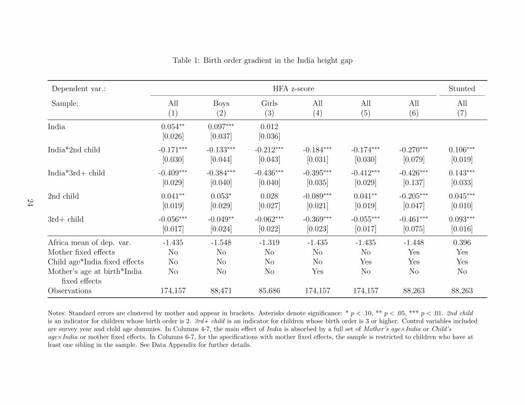
Table 1: Birth order gradient in the India height gap
Dependent var.: HFA z-score Stunted
Sample: All Boys Girls All All All All(1) (2) (3) (4) (5) (6) (7)
India 0.054∗∗ 0.097∗∗∗ 0.012[0.026] [0.037] [0.036]
India*2nd child -0.171∗∗∗ -0.133∗∗∗ -0.212∗∗∗ -0.184∗∗∗ -0.174∗∗∗ -0.270∗∗∗ 0.106∗∗∗
[0.030] [0.044] [0.043] [0.031] [0.030] [0.079] [0.019]
India*3rd+ child -0.409∗∗∗ -0.384∗∗∗ -0.436∗∗∗ -0.395∗∗∗ -0.412∗∗∗ -0.426∗∗∗ 0.143∗∗∗
[0.029] [0.040] [0.040] [0.035] [0.029] [0.137] [0.033]
2nd child 0.041∗∗ 0.053∗ 0.028 -0.089∗∗∗ 0.041∗∗ -0.205∗∗∗ 0.045∗∗∗
[0.019] [0.029] [0.027] [0.021] [0.019] [0.047] [0.010]
3rd+ child -0.056∗∗∗ -0.049∗∗ -0.062∗∗∗ -0.369∗∗∗ -0.055∗∗∗ -0.461∗∗∗ 0.093∗∗∗
[0.017] [0.024] [0.022] [0.023] [0.017] [0.075] [0.016]
Africa mean of dep. var. -1.435 -1.548 -1.319 -1.435 -1.435 -1.448 0.396Mother fixed effects No No No No No Yes YesChild age*India fixed effects No No No No Yes Yes YesMother’s age at birth*India No No No Yes No No No
fixed effectsObservations 174,157 88,471 85,686 174,157 174,157 88,263 88,263
Notes: Standard errors are clustered by mother and appear in brackets. Asterisks denote significance: * p < .10, ** p < .05, *** p < .01. 2nd childis an indicator for children whose birth order is 2. 3rd+ child is an indicator for children whose birth order is 3 or higher. Control variables includedare survey year and child age dummies. In Columns 4-7, the main effect of India is absorbed by a full set of Mother’s age×India or Child’sage×India or mother fixed effects. In Columns 6-7, for the specifications with mother fixed effects, the sample is restricted to children who have atleast one sibling in the sample. See Data Appendix for further details.
24

Table 2: Birth order gradient in infant mortality and in the effect of maternal height on child height
Deceased Deceased HFA z-score HFA z-score(1) (2) (3) (4)
Mother’s height 5.465∗∗∗
[0.180]
2nd child*Mother’s height -0.026 -0.266[0.245] [0.496]
3rd+ child*Mother’s height -0.621∗∗∗ -0.725[0.217] [0.707]
India -0.038∗∗∗ 0.477∗∗∗
[0.003] [0.028]
India*2nd child 0.005 0.015 -0.155∗∗∗ -0.282∗∗∗
[0.003] [0.014] [0.033] [0.084]
India*3rd+ child 0.013∗∗∗ 0.010 -0.374∗∗∗ -0.470∗∗∗
[0.003] [0.024] [0.031] [0.144]
2nd child -0.018∗∗∗ -0.059∗∗∗ 0.071 0.211[0.002] [0.007] [0.388] [0.785]
3rd+ child -0.013∗∗∗ -0.103∗∗∗ 0.895∗∗∗ 0.678[0.002] [0.012] [0.344] [1.120]
Africa mean of dep. var. 0.072 0.102 -1.435 -1.448Mother fixed effects No Yes No YesChild age*India fixed effects No Yes No YesObservations 199,666 91,099 172,630 87,568
Notes: Asterisks denote significance: * p < .10, ** p < .05, *** p < .01. In Columns 1-2, the sample comprises children, alive or deceased, who are orwould have been age 13 to 59 months at the time of the survey, regardless of whether anthropometric data are available. In Columns 3-4, the samplecomprises children age 1-59 months with anthropometric data. Standard errors are clustered by mother and appear in brackets. Control variablesincluded are survey year and child age dummies. See Data Appendix for further details.
25
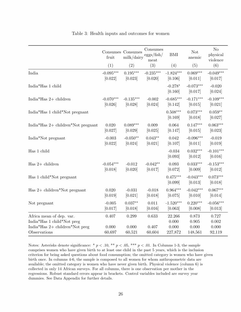
Table 3: Health inputs and outcomes for women
Consumesfruit
Consumesmilk/dairy
Consumeseggs/fish/
meatBMI
Notanemic
Nophysicalviolence
(1) (2) (3) (4) (5) (6)
India -0.095∗∗∗ 0.195∗∗∗ -0.235∗∗∗ -1.824∗∗∗ 0.069∗∗∗ -0.049∗∗∗
[0.022] [0.023] [0.020] [0.106] [0.011] [0.017]
India*Has 1 child -0.278∗ -0.073∗∗∗ -0.020[0.160] [0.017] [0.024]
India*Has 2+ children -0.070∗∗∗ -0.135∗∗∗ -0.002 -0.685∗∗∗ -0.171∗∗∗ -0.109∗∗∗
[0.026] [0.028] [0.024] [0.142] [0.015] [0.021]
India*Has 1 child*Not pregnant 0.508∗∗∗ 0.073∗∗∗ 0.059∗∗
[0.169] [0.018] [0.027]
India*Has 2+ children*Not pregnant 0.020 0.089∗∗∗ 0.009 0.064 0.147∗∗∗ 0.063∗∗∗
[0.027] [0.029] [0.025] [0.147] [0.015] [0.023]
India*Not pregnant -0.003 -0.050∗∗ 0.043∗∗ 0.042 -0.096∗∗∗ -0.019[0.022] [0.024] [0.021] [0.107] [0.011] [0.019]
Has 1 child -0.034 0.032∗∗∗ -0.101∗∗∗
[0.093] [0.012] [0.016]
Has 2+ children -0.054∗∗∗ -0.012 -0.042∗∗ 0.093 0.033∗∗∗ -0.153∗∗∗
[0.018] [0.020] [0.017] [0.072] [0.009] [0.012]
Has 1 child*Not pregnant 0.475∗∗∗ -0.043∗∗∗ 0.073∗∗∗
[0.099] [0.013] [0.018]
Has 2+ children*Not pregnant 0.020 -0.031 -0.018 0.964∗∗∗ -0.042∗∗∗ 0.067∗∗∗
[0.019] [0.021] [0.018] [0.075] [0.010] [0.014]
Not pregnant -0.005 0.037∗∗ 0.011 -1.520∗∗∗ 0.220∗∗∗ -0.056∗∗∗
[0.017] [0.018] [0.016] [0.063] [0.008] [0.013]
Africa mean of dep. var. 0.407 0.299 0.633 22.266 0.873 0.727India*Has 1 child*Not preg 0.000 0.905 0.002India*Has 2+ children*Not preg 0.000 0.000 0.407 0.000 0.000 0.000Observations 60,697 60,521 60,604 227,872 148,561 92,119
Notes: Asterisks denote significance: * p < .10, ** p < .05, *** p < .01. In Columns 1-3, the samplecomprises women who have given birth to at least one child in the past 5 years, which is the inclusioncriterion for being asked questions about food consumption; the omitted category is women who have givenbirth once. In columns 4-6, the sample is composed to all women for whom anthropometric data areavailable; the omitted category is women who have never given birth. Physical violence (column 6) iscollected in only 14 African surveys. For all columns, there is one observation per mother in theregressions. Robust standard errors appear in brackets. Control variables included are survey yeardummies. See Data Appendix for further details.
26

Table 4: Food consumption of women in India compared to their husbands
Consumes fruitConsumesmilk/dairy
Consumeseggs/fish/meat
(1) (2) (3)
Mother 0.088∗∗∗ 0.001 -0.001[0.016] [0.017] [0.012]
Mother*Has 1 child -0.044∗ -0.021 -0.012[0.025] [0.026] [0.018]
Mother*Has 2+ children -0.079∗∗∗ -0.098∗∗∗ -0.033∗∗
[0.020] [0.025] [0.016]
Mother*Has 1 child*Not pregnant 0.031 0.025 0.024[0.027] [0.029] [0.020]
Mother*Has 2+ children*Not pregnant 0.048∗∗ 0.085∗∗∗ 0.035∗
[0.022] [0.027] [0.018]
Mother*Not pregnant -0.067∗∗∗ -0.044∗∗ -0.021[0.019] [0.020] [0.014]
Has 1 child -0.027 -0.023 -0.012[0.019] [0.024] [0.016]
Has 2+ children -0.156∗∗∗ -0.165∗∗∗ -0.055∗∗∗
[0.016] [0.022] [0.015]
Has 1 child*Not pregnant 0.054∗∗ 0.035 0.028[0.022] [0.027] [0.018]
Has 2+ children*Not pregnant 0.104∗∗∗ 0.108∗∗∗ 0.033∗∗
[0.018] [0.024] [0.016]
Not pregnant -0.046∗∗∗ -0.034∗ -0.003[0.015] [0.018] [0.012]
Mother*Has 1 child*Not preg 0.292 0.764 0.157Mother*Has 2+ children*Not preg 0.001 0.250 0.785Observations 40,177 40,190 40,159
Notes: Standard errors are clustered by household and appear in brackets. Asterisks denote significance: *p < .10, ** p < .05, *** p < .01. The sample includes Indian women who have given birth to at least 1child in the past 5 years and their husbands, if both spouses answered consumption questions. The omittedcategory is men whose wives have never given birth. See Data Appendix for further details.
27

Table 5: Child health inputs
Totalprenatal
visits
Mothertook
iron sup-plements
Totaltetanusshots
Novision
problem
Deliveryat
healthfacility
Exclus.breastfed
for 6mos.
Min.acceptable
diet
Postnatalcheck
within 2mos.
Childtaking
iron pills
Totalvaccina-
tions
(1) (2) (3) (4) (5) (6) (7) (8) (9) (10)
India 1.871∗∗∗ 0.113∗∗∗ 0.510∗∗∗ 0.097∗∗∗ 0.046∗∗∗ 0.054∗∗∗ 0.026∗∗ -0.104∗∗∗ 0.016∗∗∗ 0.793∗∗∗
[0.050] [0.007] [0.015] [0.005] [0.006] [0.017] [0.012] [0.015] [0.005] [0.043]
India*2nd child -0.497∗∗∗ -0.021∗∗∗ 0.005 -0.007 -0.035∗∗∗ 0.036∗ -0.005 -0.017 -0.002 -0.230∗∗∗
[0.063] [0.008] [0.017] [0.005] [0.007] [0.021] [0.010] [0.013] [0.005] [0.043]
India*3rd+ child -2.007∗∗∗ -0.173∗∗∗ -0.133∗∗∗ -0.022∗∗∗ -0.180∗∗∗ 0.051∗∗∗ -0.023∗∗∗ -0.035∗∗∗ -0.002 -1.158∗∗∗
[0.054] [0.007] [0.016] [0.005] [0.007] [0.019] [0.008] [0.011] [0.005] [0.046]
2nd child -0.165∗∗∗ -0.016∗∗∗ -0.133∗∗∗ -0.007∗ -0.090∗∗∗ -0.008 -0.002 0.024∗∗ -0.006 -0.075∗∗∗
[0.034] [0.005] [0.013] [0.004] [0.004] [0.011] [0.007] [0.010] [0.004] [0.029]
3rd+ child -0.729∗∗∗ -0.056∗∗∗ -0.343∗∗∗ -0.039∗∗∗ -0.199∗∗∗ -0.001 -0.019∗∗∗ 0.002 -0.031∗∗∗ -0.446∗∗∗
[0.027] [0.004] [0.010] [0.003] [0.004] [0.009] [0.005] [0.008] [0.004] [0.026]
Africa mean of dep. var. 3.828 0.617 1.406 0.854 0.469 0.313 0.130 0.297 0.112 6.187Observations 120,570 122,977 122,530 120,119 173,772 19,936 37,710 39,248 95,986 127,544
Notes: Standard errors are clustered by household and appear in brackets. Asterisks denote significance: * p < .10, ** p < .05, *** p < .01. Controlvariables included are survey year and child age dummies. In Column 1-5, the sample includes children age 1-59 months; whether the mother tookiron pills is collected in 10 African surveys. Data on postnatal outcomes are available for a subset of children in the sample: In Column 6, thesample comprises the youngest child from each family, age 1-6 months. In Column 7, the sample comprises the youngest child from each family, age7-24 months; data to construct minimum acceptable diet in a comparable way to India is available in 17 African surveys. In Column 8, the samplecomprises the youngest child from each family, age 1-59 months; postnatal check within 2 months is collected in 13 African surveys. In Columns9-10, the sample includes children age 1-59 months. See Data Appendix for further details.
28

Table 6: Child morbidity and school enrollment
Notanemic
Nodiarrhea in
last 2weeks
No feveror coughin last 2weeks
Years ofeducation
(1) (2) (3) (4)
India 0.149∗∗∗ 0.062∗∗∗ 0.089∗∗∗ 1.650∗∗∗
[0.008] [0.004] [0.006] [0.018]
India*2nd child -0.020∗∗ -0.001 0.001 -0.014[0.009] [0.005] [0.006] [0.018]
India*3rd+ child -0.053∗∗∗ -0.008∗ 0.009 -0.261∗∗∗
[0.008] [0.004] [0.006] [0.020]
2nd child -0.005 0.003 0.016∗∗∗ -0.030∗∗∗
[0.006] [0.003] [0.004] [0.011]
3rd+ child -0.022∗∗∗ -0.003 0.011∗∗∗ -0.240∗∗∗
[0.005] [0.003] [0.003] [0.011]
Africa mean of dep. var. 0.567 0.843 0.664 1.999Observations 91,661 173,570 173,316 265,352
Notes: Standard errors are clustered by household and appear in brackets. Asterisks denote significance: * p < .10, ** p < .05, *** p < .01. Controlvariables included are survey year and child age dummies (measured in months in columns 1-3 and years in column 4). In columns 1-3, the samplecomprises children age 1-59 months. In column 4, the sample comprises children age 7 to 17 years at the time of the survey. See Data Appendix forfurther details.
29

Table 7: Birth order gradient in child height, by gender of older siblings
HFA z-score HFA z-score(1) (2)
India -0.047∗∗ -0.085[0.022] [0.056]
Girl 0.230∗∗∗ 0.205∗∗∗
[0.013] [0.040]
India*Girl -0.183∗∗∗ -0.160∗∗
[0.023] [0.062]
Firstborn is a girl 0.021[0.042]
India*Firstborn is a girl 0.078[0.063]
India*Girl*Firstborn is a girl -0.126[0.090]
Girl*Firstborn is a girl 0.032[0.057]
Sample All children2nd bornchildren
Africa mean of dep. var. -1.435 -1.375Observations 174,157 36,842
Notes: Standard errors are clustered by household and appear in brackets. Asterisks denote significance: *p < .10, ** p < .05, *** p < .01. Control variables included are survey year and child age dummies. Thesample includes all children age 1-59 months in Column 1 and all second-born children age 1-59 months inColumn 2. See Data Appendix for further details.
30

Appendix Table 1: Summary statistics
Indiasubsample
Africasubsample
Indiasubsample
Africasubsample
Child’s age (months) 30.051 28.062 No vision problem 0.892 0.854[16.872] [17.026] [0.31] [0.353]
Mother’s age at birth (years) 24.767 26.954 Delivery at health facility 0.449 0.469[5.239] [6.857] [0.497] [0.499]
Girl 0.479 0.496 Exclusively breastfed for 6 mos. 0.4 0.313[0.5] [0.5] [0.49] [0.464]
Mother’s total children born 2.745 3.876 Minimum acceptable diet 0.095 0.13[1.829] [2.543] [0.294] [0.336]
HFA z-score -1.575 -1.435 Postnatal check within 2 mos. 0.092 0.297[2.114] [2.466] [0.289] [0.457]
WFA z-score -1.546 -0.869 Child taking iron pills 0.055 0.112[1.494] [1.805] [0.228] [0.315]
WFH z-score -0.95 -0.057 Child’s total vaccinations 6.593 6.187[1.998] [2.695] [2.809] [3.149]
Mother’s BMI 21.138 23.133 Child not anemic 0.613 0.567[3.125] [3.622] [0.487] [0.495]
Mother’s height 1.519 1.583 No diarrhea in last 2 weeks 0.905 0.843[0.058] [0.069] [0.293] [0.364]
Mother not anemic 0.687 0.702 No fever or cough in last 2 weeks 0.772 0.664[0.464] [0.457] [0.42] [0.472]
Mother consumes fruit 0.177 0.4 No physical violence 0.719 0.741[0.337] [0.49] [0.45] [0.438]
Mother consumes milk/dairy 0.373 0.282 Child stunted 0.414 0.39[0.463] [0.45] [0.493] [0.488]
Mother consumes egg/fish/meat 0.128 0.642 Child deceased 0.05 0.072[0.27] [0.479] [0.217] [0.259]
Total prenatal visits 4.031 3.828 Child’s years of schooling 3.613 1.999[3.483] [3.095] [2.556] [2.097]
Took iron supplements 0.687 0.617 ln(GDP/cap, birth year) 7.735 6.891[0.464] [0.486] [0.125] [0.653]
Total tetanus shots 1.867 1.406[0.941] [1.202]
Notes: Mean of the specified variables are calculated separately for the Indian subsample and the African subsample. Standard deviations appear inbrackets.
31
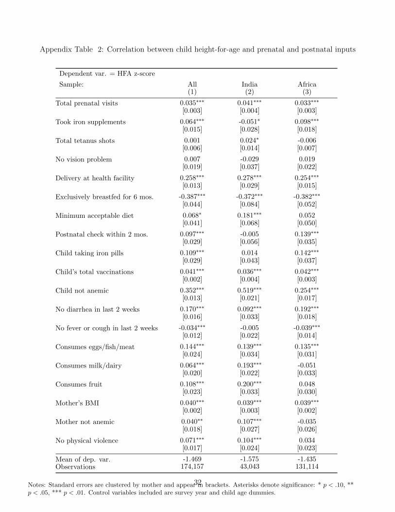
Appendix Table 2: Correlation between child height-for-age and prenatal and postnatal inputs
Dependent var. = HFA z-score
Sample: All India Africa(1) (2) (3)
Total prenatal visits 0.035∗∗∗ 0.041∗∗∗ 0.033∗∗∗
[0.003] [0.004] [0.003]
Took iron supplements 0.064∗∗∗ -0.051∗ 0.098∗∗∗
[0.015] [0.028] [0.018]
Total tetanus shots 0.001 0.024∗ -0.006[0.006] [0.014] [0.007]
No vision problem 0.007 -0.029 0.019[0.019] [0.037] [0.022]
Delivery at health facility 0.258∗∗∗ 0.278∗∗∗ 0.254∗∗∗
[0.013] [0.029] [0.015]
Exclusively breastfed for 6 mos. -0.387∗∗∗ -0.372∗∗∗ -0.382∗∗∗
[0.044] [0.084] [0.052]
Minimum acceptable diet 0.068∗ 0.181∗∗∗ 0.052[0.041] [0.068] [0.050]
Postnatal check within 2 mos. 0.097∗∗∗ -0.005 0.139∗∗∗
[0.029] [0.056] [0.035]
Child taking iron pills 0.109∗∗∗ 0.014 0.142∗∗∗
[0.029] [0.043] [0.037]
Child’s total vaccinations 0.041∗∗∗ 0.036∗∗∗ 0.042∗∗∗
[0.002] [0.004] [0.003]
Child not anemic 0.352∗∗∗ 0.519∗∗∗ 0.254∗∗∗
[0.013] [0.021] [0.017]
No diarrhea in last 2 weeks 0.170∗∗∗ 0.092∗∗∗ 0.192∗∗∗
[0.016] [0.033] [0.018]
No fever or cough in last 2 weeks -0.034∗∗∗ -0.005 -0.039∗∗∗
[0.012] [0.022] [0.014]
Consumes eggs/fish/meat 0.144∗∗∗ 0.139∗∗∗ 0.135∗∗∗
[0.024] [0.034] [0.031]
Consumes milk/dairy 0.064∗∗∗ 0.193∗∗∗ -0.051[0.020] [0.022] [0.033]
Consumes fruit 0.108∗∗∗ 0.200∗∗∗ 0.048[0.023] [0.033] [0.030]
Mother’s BMI 0.040∗∗∗ 0.039∗∗∗ 0.039∗∗∗
[0.002] [0.003] [0.002]
Mother not anemic 0.040∗∗ 0.107∗∗∗ -0.035[0.018] [0.027] [0.026]
No physical violence 0.071∗∗∗ 0.104∗∗∗ 0.034[0.017] [0.024] [0.023]
Mean of dep. var. -1.469 -1.575 -1.435Observations 174,157 43,043 131,114
Notes: Standard errors are clustered by mother and appear in brackets. Asterisks denote significance: * p < .10, **p < .05, *** p < .01. Control variables included are survey year and child age dummies.
32
Appendix Table 3: Can covariates account for the India height gap?
Dependent var. = HFA z-score
Explanatory var. : None Economic characteristics Environmental features Mother characteristics Parents’ height
Householdwealthindex
Ruralhouse-hold
Opendefeca-
tion
Access topipedwater
Motheris literate
Empower-mentindex
Mother’sheight
Father’sheight
(1) (2) (3) (4) (5) (6) (7) (8) (9)
India -0.135∗∗∗ -0.363∗∗∗ -0.189∗∗∗ -0.085∗∗∗ -0.203∗∗∗ -0.282∗∗∗ -0.208∗∗∗ 0.312∗∗∗ -0.107∗∗
[0.019] [0.019] [0.019] [0.019] [0.019] [0.019] [0.020] [0.020] [0.044]
Explanatory var. 0.127∗∗∗ -0.512∗∗∗ -0.358∗∗∗ 0.425∗∗∗ 0.449∗∗∗ 0.266∗∗∗ 5.138∗∗∗ 4.329∗∗∗
[0.002] [0.012] [0.012] [0.012] [0.012] [0.017] [0.093] [0.224]
Explanatory var. :Africa mean 4.299 0.719 0.322 0.260 0.477 0.492 1.583 1.693India mean 6.346 0.632 0.456 0.413 0.563 0.611 1.519 1.642
Observations 174,157 174,157 174,157 168,840 168,688 172,865 139,248 172,630 23,047
Notes: Standard errors are clustered by mother and appear in brackets. Asterisks denote significance: * p < .10, ** p < .05, *** p < .01. Controlvariables included are survey year, child age, and child gender dummies. Columns 2-9 include the explanatory variable specified in the columnheading. Father’s height is collected in India and 4 African surveys.
33

Appendix Table 4: Birth order gradient in child weight + height outcomes by child age
Dependent var.: WFA z-score WFH z-score HFA z-score
Sample: All All All AllAge 1-6
mos.Age 7-59
mos.Age 1-6
mos.Age 7-59
mos.(1) (2) (3) (4) (5) (6) (7) (8)
India -0.313∗∗∗ -0.493∗∗∗ -0.392∗∗∗ -0.106∗∗∗ -0.200∗∗ 0.079∗∗∗
[0.019] [0.027] [0.067] [0.019] [0.101] [0.026]
India*2nd child -0.146∗∗∗ -0.213∗∗∗ -0.045 -0.071 -0.099 -0.175∗∗∗
[0.022] [0.058] [0.033] [0.083] [0.129] [0.030]
India*3rd+ child -0.329∗∗∗ -0.305∗∗∗ -0.113∗∗∗ -0.095 -0.310∗∗∗ -0.410∗∗∗
[0.021] [0.095] [0.031] [0.141] [0.113] [0.029]
2nd child 0.027∗ 0.013 -0.024 0.195∗∗∗ 0.172∗∗ 0.021[0.015] [0.035] [0.024] [0.054] [0.074] [0.020]
3rd+ child -0.098∗∗∗ -0.058 -0.111∗∗∗ 0.331∗∗∗ 0.239∗∗∗ -0.098∗∗∗
[0.013] [0.054] [0.021] [0.085] [0.060] [0.017]
Africa mean of dep. var. -0.869 -0.911 -0.057 -0.101 0.590 -1.713 0.590 -1.713Observations 174,157 88,263 174,157 88,263 20,023 154,134 20,023 154,134
Notes: Standard errors are clustered by mother and appear in brackets. Asterisks denote significance: * p < .10, ** p < .05, *** p < .01. Controlvariables included are survey year and child age dummies.
34

Appendix Table 5: Effect of open defecation on child height, by birth order
HFA z-score HFA z-score(1) (2)
Open defecation -0.441∗∗∗
[0.024]
2nd child*Open defecation 0.060∗ -0.032[0.033] [0.068]
3rd+ child*Open defecation 0.154∗∗∗ -0.078[0.029] [0.098]
India 0.100∗∗∗
[0.027]
India*2nd child -0.175∗∗∗ -0.255∗∗∗
[0.031] [0.081]
India*3rd+ child -0.384∗∗∗ -0.389∗∗∗
[0.030] [0.140]
2nd child 0.028 -0.184∗∗∗
[0.021] [0.051]
3rd+ child -0.088∗∗∗ -0.427∗∗∗
[0.019] [0.081]
Africa mean of dep. var. -1.435 -1.448Mother fixed effects No YesChild age*India fixed effects No YesObservations 168,840 86,172
Notes: Standard errors are clustered by mother and appear in brackets. Asterisks denote significance: *p < .10, ** p < .05, *** p < .01. Control variables included are survey year and child age in monthsdummies. Open defecation is a dummy variable that equals 1 if the mother reports that the household hasno toilet facility.
35

Appendix Table 6: Fertility stopping patterns in India compared to Africa
Has 2+ children Has 3+ children(1) (2)
India -0.103∗∗∗ -0.232∗∗∗
[0.004] [0.007]
Firstborn is a girl -0.003[0.003]
India*Firstborn is a girl 0.037∗∗∗
[0.005]
First and second borns are girls 0.000[0.004]
First and second borns include a boy and a girl -0.003[0.004]
India*First and second borns are girls 0.136∗∗∗
[0.009]
India*First and second borns include a boy and a girl 0.019∗∗
[0.008]
Africa mean of dep. var. 0.810 0.771
Sample AllMother has 2+
childrenObservations 128,129 101,119
Notes: Robust standard errors appear in brackets. Asterisks denote significance: * p < .10, ** p < .05, ***p < .01. Control variables included are survey year and child age in months dummies.
36

Data Appendix
DHS surveys usedThe data sets included from Sub-Saharan Africa are Democratic Republic of the Congo 2007 (V),
Republic of the Congo (Brazzaville) 2005 (V), Cameroon 2004 (IV), Chad 2004 (IV), Ethiopia 2005 (V),Ghana 2008 (V), Guinea 2005 (V), Kenya 2008-9 (V), Liberia 2007 (V), Lesotho 2004 (IV), Lesotho 2009(VI), Madagascar 2003-4 (IV), Mali 2006 (V), Malawi 2004 (IV), Niger 2006 (V), Nigeria 2008 (V),Namibia 2006-7 (V), Rwanda 2005 (V), Sierra Leone 2008 (V), Senegal 2005 (IV), Sao Tome 2008 (V),Swaziland 2006-7 (V), Tanzania 2004-5 (IV), Tanzania 2010 (VI), Uganda 2006 (V), Zambia 2007 (V), andZimbabwe 2005-6 (V). The DHS questionnaire version (IV, V, or VI) is given in parentheses. The data setincluded from India is India 2005-6 (NFHS-3). For the analysis on child’s educational attainment, 2additional surveys are included, Benin 2006 (V) and Madagascar 2008-9 (V).
Height-for-age, weight-for-age, and weight-for-height z-scoresFor comparing height and weight across children of different gender and age, we create normalized
variables using the World Heath Organization (WHO) method (WHO Multicentre Growth ReferenceStudy Group, 2006). The WHO provides the distribution of height, weight and weight-for-height separatelyfor boys and girls, by age in months from a reference population of children from Brazil, Ghana, India,Norway, Oman and the United States. Since child height and weight have a skewed distribution, the WHOrecommends a restricted application of the LMS method for fitting the skewed data adequately by using aBox-Cox normal distribution. The formula used is as follows:
z-score =(observed value/M)L−1
L× S
The WHO provides the values of M , L and S for each reference population by gender and age. M is thereference median value for estimating the population mean, L is the power used to transform the data toremove skewness, and S is the coefficient of variation.
Child ageFor all children whose anthropometric data were recorded, the DHS also provides the measurement
date. Our child age variable is in months, and is constructed by calculating the number of days elapsedbetween the child’s birth and the measurement date, and then converting this age into months. When werefer to a child as n months old, we mean the child is in its nth month of life such that a child who is oneweek old is in its 1st month of life, hence 1 month old.
Birth orderChildren of multiple births, such as twins or triplets, are assigned the same birth order. For a child
born subsequent to a multiple birth, birth order is incremented by the size of the multiple birth. Forexample, the next child born after firstborn twins is birth order 3. We construct birth order based onchildren ever born, not on only surviving children.
Maternal outcomesMother consumes fruit, milk/dairly, egg/fish/meat is constructed based on the DHS and NFHS
variables on mother’s food consumption. Mother’s food consumption is available in 10 African DHS’s(Ghana 2008, Liberia 2007, Nigeria 2008, Namibia 2006-7, Sierra Leone 2008, Sao Tome 2008, Swaziland2006-7, Uganda 2006, Zambia 2007, and Zimbabwe 2005-6). These surveys asked detailed questions aboutthe food and liquid items consumed in the last 24 hours to mothers who have given birth in the last 3years. Based on this, we created an indicator for whether mother consumed the specified food item in theprevious day. For instance, eggs, fish, meat were 3 separate questions, so we created an indicator forwhether mothers consumed any one of the 3 food groups for those who answered all three questions.NFHS-3 had related but different questions about mother’s food consumption. They asked all womenliving with a child younger than 36 months about how frequently they consume the specified food group.
37

Hence we coded daily consumption as 1, weekly consumption as 1/7, and occasionally and never as 0 tomake the variable comparable to the one from the African DHS’s. We then restrict the sample to womenwho are living with a child younger than 36 months to ensure that the sample inclusion criterion isconsistent across surveys. NFHS-3 also asked the same set of consumption related questions to fathers inthe Men’s Questionnaire, and father’s consumption is coded the same way.
Mother’s BMI is collected for all women in some DHS’s and NFHS, and collected for a smaller sampleof women whose household was selected for the men’s survey in the other DHS’s. Hence, BMI informationis available in 26 African DHS’s and the NFHS. Chad 2004 is excluded because it only collects BMIinformation from women who had a birth in the last 3 years. Mother’s BMI is the women’s weight inkilograms divided by her height in meters squared. We restrict the sample to women who have given birthin the last 5 years or never given birth.
Mother’s anemia is collected for all women in some DHS’s and NFHS, and collected for a smallersample of women whose household was selected for hemoglobin testing in other DHS’s. Many DHS’scollected anemia for smaller subsamples or did not collect anemia information at all, although theycollected BMI of all women. Hence, anemia information is available in 21 African DHS’s and the NFHS. Itis the measure of whether the women has severe or moderate anemia according to the DHS standards.Levels below 7.0 g/dl are regarded as severe anemia and levels between 7.1g/dl and 9.9g/dl are regarded asmoderate anemia. We restrict the sample to women who have given birth in the last 5 years or never givenbirth.
Any physical violence is collected for all married women who are selected for the domestic violencemodule. It is available in 14 African DHS’s (Democratic Republic of the Congo 2007, Cameroon 2004,Ghana 2008, Kenya 2008-9, Liberia 2007, Mali 2006, Malawi 2004, Nigeria 2008, Rwanda 2005, Sao Tome2008, Tanzania 2010, Uganda 2006, Zambia 2007, and Zimbabwe 2005-6) and the NFHS. It is the mother’sself-report of whether she experienced any physical violence from the current spouse.
Prenatal variablesTotal prenatal visits is collected for the most recent birth in the past 5 years. Hence, our sample is
restricted to youngest living child from each family for this variable. It is available in all 27 African DHS’sand the NFHS. It is the mother’s self-report of the total number of prenatal visits during the pregnancy. Itis 0 if the mother never went for a prenatal visit, and the maximum number of visits is top-coded at 20.
Mother took iron supplements is collected for the most recent birth in the past 5 years. It is availablein all 27 African DHS’s and the NFHS. It is the mother’s self-report of whether she took iron supplementsduring the pregnancy of her youngest living child.
Total tetanus shots is collected for the most recent birth in the past 5 years. The exception isDemocratic Republic of the Congo 2007 which collected it for all births in the past 5 years; we restrict thesample to the most recent birth to ensure consistency. It is available in all 27 African DHS’s and theNFHS. It is the mother’s self-report of the number of tetanus toxoid injections given during the pregnancyto avoid convulsions after birth. The DHS recorded having more than 7 injections as 7.
Any vision problem is constructed from 2 variables related to vision problems, collected for the mostrecent birth in the past 5 years. It is available in 26 African DHS’s and the NFHS, but not available inLiberia 2007. Mothers reported whether they experienced difficulty with daylight vision (a sign ofpre-eclampsia), and also whether they experienced night blindness (a sign of vitamin A deficiency) duringtheir most recent pregnancy. Any vision problem is constructed for mothers that answered both questions,and it equals 1 if they experienced either of the problems.
Delivery at home is collected for all births in the past 5 years. It is available in all 27 African DHS’sand the NFHS. It is the mother’s self-report of whether the child was delivered at her home, her parents’home, traditional birth attendant’s home or some other home, in other words, not in a health facility.
Postnatal variablesExclusively breastfed is constructed based on the mother’s recall of liquid and food items given to the
child in the 24 hours before the survey, and her self-report of whether the child is currently being breastfed.Both pieces of information are available for all births in the last 5 years in the full sample of 27 AfricanDHS’s and the NFHS. Since WHO recommends exclusive breastfeeding for children age 1-6 months, we
38

restrict the sample to children age 1-6 months, which gives us the sample of youngest child in family. Thevariable takes the value 1 if the child is currently being breastfed and was not given any liquid or foodother than breast milk.
Minimum acceptable diet is constructed based on the mother’s recall of liquid and food items given tothe child in the 24 hours before the survey, the frequency of feeding, and whether the child is currentlybeing breastfed. For children age 7-24 months, WHO defines ’minimum dietary diversity’ as having at least4 of following 7 food groups: grains, roots and tubers; legumes and nuts; dairy products; flesh foods (meat,fish, poultry and liver/organ meats); eggs; vitamin-A rich fruits and vegetables; other fruits and vegetables.However, DHS questionnaires often group egg and meat together and do not differentiate vitamin A richfruits/vegetables and regular fruits/vegetables. Hence, we modified the definition of minimum dietarydiversity as having at least 4 of the following 5 food groups: grains, roots and tubers; legumes and nuts;dairy products; flesh foods (meat, fish, poultry and liver/organ meats) or eggs; fruits and vegetables. WHOdefines minimum meal frequency as 2 times for breastfed infants 6-8 months old, 3 times for breastfedchildren 9-23 months old, and 4 times for non-breastfed children 6-23 months old. Minimum acceptablediet is meeting the minimum dietary diversity and the minimum meal frequency during the previous day.In addition, non-breastfed children should also receive a milk feeding, which we modify from WHO’srecommendation of 2 milk feedings due to the lack of milk feeding frequency data. 17 African DHS’s andthe NFHS contain all necessary variables to determine whether the child has minimum acceptable diet.Since individual DHS’s and NFHS differ in the criteria for collecting the necessary information, we restrictthe sample to meet the most exclusive criteria, namely the youngest child in the family. The sample age isalso restricted to age 7-24 months to meet the WHO’s guideline.
Postnatal check within 2 months is collected for the most recent birth in the past 5 years. It isavailable in 13 African DHS’s (Ghana 2008, Kenya 2008-9, Liberia 2007, Lesotho 2009, Nigeria 2008,Namibia 2006-7, Sierra Leone 2008, Sao Tome 2008, Swaziland 2006-7, Tanzania 2010, Uganda 2006,Zambia 2007, and Zimbabwe 2005-6) as well as the NFHS. It is the mother’s self-report of whether thechild received a postnatal check within 2 months after it was born.
Child taking iron pills is collected for all births in the past 5 years. It is available in 10 African DHS’s(Ghana 2008, Kenya 2008-9, Liberia 2007, Nigeria 2008, Namibia 2006-7, Sierra Leone 2008, Sao Tome2008, Swaziland 2006-7, Tanzania 2010, and Uganda 2006) as well as the NFHS. It is the mother’sself-report of whether the child is currently taking iron pills.
Child’s total vaccinations is collected for all births in the past 5 years. It is available in all 27 AfricanDHS’s and the NFHS. It is the mother’s self-report of the total number of vaccinations the child hasreceived to date. The vaccines counted include BCG, 3 doses of DPT, 4 doses of polio, and measles, sochild’s total vaccinations is 9 if the child received all vaccines. The sample is restricted to children age13-59 months since the recommended age for the vaccinations is up to age 12 months.
Child morbidity variablesChild anemic is collected for all births in the past 5 years. It is available in 21 African DHS’s and the
NFHS. It is the measure of whether the child is moderately or severely anemic, determined by the child’sblood sample collected. Levels below 7.0 g/dl are considered as severe anemia and levels between 7.1g/dland 9.9g/dl are considered as moderate anemia.
Diarrhea in last 2 weeks is collected for all births in the past 5 years. It is available in all 27 AfricanDHS’s and the NFHS. It is the mother’s self-report of whether the child had diarrhea in the 2 weeks beforethe survey.
Fever or cough in last 2 weeks is constructed from 2 questions on child’s recent health. Mothersreported whether the child had fever in the 2 weeks before the survey, and also whether the child hadcough in the last 2 weeks. The two variables are collected for all births in the past 5 years, and is availablein the full sample of 27 African DHS’s and the NFHS. So the variable, Fever or cough in last 2 weeks, takesthe value 1 if the child had either fever or cough in the last 2 weeks.
Other variablesMother’s height is measured for mothers of children born in the 5 years preceding the survey. It is
available in all 27 African DHS’s and the NFHS. Mother’s height is converted to meters and is coded as
39

missing if the height is less than 1.25 meters.Father’s height is measured for fathers of children in some surveys. However, the survey must also
provide the line number of fathers in order for fathers’ information to be correctly matched to children’sinformation. 4 African DHS’s (Lesotho 2009, Sao Tome 2008, Swaziland 2006-7, Uganda 2006) as well asthe NFHS provide both pieces of information. Father’s height is converted to meters and is coded asmissing if the height is less than 1.25 meters.
Household wealth index is constructed based on basic household asset data and available for all birthsin the full sample of 27 African DHS’s and the NFHS. It is calculated as the sum of the following 14indicators of household assets: Non-surface source of drinking water (surface water includes rivers, spring,pond, etc.); flush toilet; electricity; radio, television; refrigerator; bicycle; motorcycle; car; telephone;non-natural floor material (natural materials include mud/clay/earth, sand, dung, etc.); non-natural roofmaterial (natural materials include no roofs, leaves, mud, etc.); non-natural wall material (naturalmaterials include no walls, cane/palm/trunks, grass/reeds, etc.); and non-natural cooking fuel (naturalmaterials include dung, straw/shrubs/grass, etc.). If the information for some of the 14 items are missingfor a household, the missing values are replaced with the African mean for African DHS’s, and the Indianmean for the NFHS.
Rural household is available for all births in the past 5 years in the full sample of 27 African DHS’s andthe NFHS. It is a DHS recoded variable of whether the child is living in a rural area.
Open defecation is available for all births in the past 5 years in the full sample of 27 African DHS’s andthe NFHS. It is the mother’s self-report of whether the household has no toilet facility.
Access to piped water is available for all births in the past 5 years in the full sample of 27 AfricanDHS’s and the NFHS. It is the mother’s self-report of whether the household has access to piped water.
Mother is literate is available for all births in the past 5 years in the full sample of 27 African DHS’sand the NFHS. It is the mother’s self-report of whether she can read in any language.
Empowerment index is constructed based on four variables about the woman’s say in householddecision-making in different domains: health, large purchases, daily purchases, and visiting family. It isavailable for all births in the full sample of 27 African DHS’s and the NFHS. Two other decision-makingvariables are available in only some surveys and hence excluded: food preparation is excluded in India andhow to spend husband’s earnings is excluded in the majority of African DHS’s. Binaries were created foreach of the four key variables for whether or not the woman had a say, either alone or with someone else, inmaking that decision. The index is the sum of these binaries and then re-scaled to [0,1].
Infant mortality is an indicator for whether the child is deceased is collected for all births in the past 5years. It is available in all 27 African DHS’s and the NFHS. It is the mother’s self-report of whether thechild is deceased. The sample is restricted to children age 13-59, as infant mortality is only defined forchildren over 1 year of age.
Children’s years of education uses DHS data on years of schooling of household members aged 7 to 14.This analysis includes 2 additional DHS data from Sub-Saharan Africa, which were previously excludedbecause they did not provide anthropometric data. Years of schooling data are obtained from the DHSHousehold Member Recode file, and birth order data are obtained the Birth Recode file. Only thosechildren who can be linked across the two files (i.e., have non-missing values of their own and theirmother’s line number variable in both files) are included. Furthermore, if the reported age of the child inthe two data sets differs by more than 3 years, we exclude the child from the analysis because either theage or line number variable is likely incorrect. Thus, the education sample includes children that can bematched across files whose age, gender, and years of education are not missing, who are aged 7-14 years,and who are from India or Sub-Saharan Africa. Age 6 or 7 is the standard school entry age in most of thecountries in the sample. The DHS asks for each household member’s highest education level attained,excluding preschool. Based on the highest level of schooling completed and the duration of each level ofschooling by country, we compute the total years of schooling the child completed. If the differencebetween the child’s age and his or her years of schooling is less than 4 years, implying he or she enteredprimary school before age 4, we top-code years of schooling at the child’s age minus 4 because the reportedvalue is likely erroneous.
40