Embed Size (px)
Citation preview

An Introductory Graph TheoryCurriculum
By Craig Swinyard
Under the direction of Dr. John S. Caughman
In partial fulfillment of the requirements for the degree of:
Masters of Science in Teaching Mathematics
Portland State UniversityDepartment of Mathematics and Statistics
Fall, 2002
1

Abstract
The fundamentals of graph theory are accessible to students who have not taken the calculus sequence. Unfortunately, most college students do not have the opportunity to explore graph theory until they have completed the entire calculus sequence. The report that follows is a description of the curriculum that I created and tested on a collection of students who had at most one quarter of calculus experience. The curriculum presented below includes ready-made activities that develop problem-solving skills while addressing some key ideas in graph theory. Following the curriculum, I have included an analysis of the evaluations turned in by the test group.
2

Chapter 1
Introduction
Section 1.1 – A Brief History of Graph Theory
Few subjects in mathematics have as specified an origin as graph theory. Graph theory originated with the Koenigsberg Bridge Problem, which Leonhard Euler (1707-1783) solved in 1736. The problem is stated as follows:
The City of Koenigsberg (formerly of Germany, now part of Russia) consists of two islands and two banks of the Pregel River (the upper bank and the lower bank). Between these four land masses there were seven decorative bridges, as seen in the map below. As legend has it, the people of Koenigsberg wondered if a route could be found such that a person could leave his or her house, walk across all seven bridges in the town exactly once, and return home (West, 2001, pp.1-2).
Euler’s solution centered on the fact that for such a route to exist, all land masses must have an even number of bridges extending to them. This would allow for a person to both enter and leave a land mass each time they visit it. An odd number of bridges attaching to a land mass would lead to a person getting “stuck” eventually. In Koenigsberg, all land masses have an odd number of bridges. Thus, Euler proved that a route of the desired kind cannot exist. An important topic in graph theory, Eulerian circuits, gets its name from the solution of this problem.
In particular, an Eulerian circuit in a graph is a circuit that traverses every edge in the graph exactly once. A graph is Eulerian if it has an Eulerian circuit. Euler concluded that for a graph to be Eulerian, it must be connected and every vertex must have even degree. Graph A is an example of an Eulerian graph. Graph B is an example of a graph that is not Eulerian.
3

The reader is probably familiar with a popular puzzle where one is asked to trace all the lines of a given diagram without picking up the pencil and without retracing any already existing lines. This is precisely the problem of finding an Eulerian circuit.
Applications of Eulerian circuits abound. For example, Eulerian circuits are obviously desirable in the deployment of street sweepers, snowplows and mail carriers. In these applications, traversing a street more than once is a waste of resources. Thus, Eulerian circuits represent optimal solutions in terms of conserving resources.
In 1758, over two decades after resolving the Koenigsberg Bridge problem, Euler made his second major contribution to the subject of graph theory with his formula for planar graphs. Planar graphs are graphs that can be drawn on the plane in such a way that no two edges cross. Such a drawing is called a planar drawing of the graph. For example, graph D is a planar drawing of graph C.
Something to note about planar drawings is that the graph clearly separates the plane into different enclosed regions or faces. For instance, in graph D above, the graph produces four faces (three “inner” faces and one “outer” face).
Euler proved that in a planar drawing, the number of vertices minus the number of edges plus the number of faces is always equal to two. In short, n – e + f = 2, where n stands for the number of vertices, e stands for the number of edges, and f stands for the number of faces. (West, 2001, p.241) For example, in graph B above, n = 4, e = 6, and f = 4. And thus, 4-6+4 = 2. This formula also has extensions beyond planar drawings to graphs drawn on more general surfaces.
4
Graph BGraph A
Graph DGraph C

As with Eulerian circuits, planarity also has many modern day applications. For example, in the circuitry of a computer chip, it is necessary that wires do not cross. If a circuitry graph has no planar drawing the chip must be built with more than one layer of silicon. A planar drawing of the graph representing the circuitry of the computer chip is therefore optimal.
Another problem concerning planar graphs was addressed nearly a hundred years after Euler. During the early 1850’s, Francis Guthrie (1831-1899) was the first to work on the Four Color Conjecture (Grimaldi, 1984, pp. 598-99). The Four Color Conjecture states that any planar graph can be properly colored using four or fewer colors. By properly colored, we mean that each vertex in the graph is assigned a color such that no two adjacent vertices have the same color.
This conjecture was not proven until 1977, when Appel, Haken, and Koch used a computer to prove the conjecture. The essential role that the computer played in this proof raised quite a controversy. The proof was based on an algorithm that allowed the computer to calculate the chromatic number of an immensely large number of graphs. Although most mathematicians accept the conjecture as proven, the search for a simpler proof remains the topic of much current research (West, 2001, p.260).
The Four Color Theorem opened the door to the broad topic of graph coloring, a topic with far reaching consequences. For example, graph coloring approaches are used in the making of maps, the assignment of work crews, and the scheduling of final exams at large colleges and universities.
The end of the 1850’s saw William Rowan Hamilton (1805-1865) contribute the idea of Hamiltonian cycles to the young subject of graph theory. Similar to Eulerian circuits, Hamiltonian cycles must visit each vertex in the graph only once before returning to the initial vertex. Notice that the emphasis is on visiting the vertices rather than the edges. Graph E below has a Hamiltonian cycle (start at vertex A and visit each vertex in alphabetical order); Graph F does not (West, 2001, p.286).
5
Graph FGraph E
C
B D
A E
T
L
J
H
FS
G
IK
M
O P
QRN

Hamiltonian cycles are useful in various operations research problems. For instance, in the routing of a delivery truck that must supply a chain of stores with goods, a Hamiltonian cycle is desirable (Tucker, 2002, p.60). Closely related to the topic of Hamiltonian cycles is the Traveling Salesman problem, one of the most famous problems in graph theory. This problem seeks an optimal route for a salesman who is planning to visit multiple cities. The goal is to find a route that minimizes the cost of travel, based on the distance between the cities. Unlike the Eulerian circuit problem, however, the Hamiltonian cycle problem and the Traveling Salesman problem do not have such concise solutions. Improving the efficiency of currently used algorithms is still a focus of intense study.
Despite the contributions in the 1700 and 1800’s, it was not until 1936 that the first graph theory text, written by Denes Konig (1884-1944), emerged (Johnsonbaugh, 2001, p.263). Over the past sixty years, there has been a great deal of exploration in the area of graph theory. Its popularity has increased due to its many modern day applications including those mentioned previously, as well as its use in chemistry, biology, linguistics, and business (Rosen, 1999, p.x). Furthermore, the rise of the computer industry has spurred interest in graph theory for two reasons. First, the development of computers has greatly increased the ability to solve what otherwise would be unmanageable problems (Grimaldi, 1984, p.599). Second, the complexity of the inner workings of a computer has motivated many new problems in graph theory, such as the computer chip problem described above.
As population rises, graph theory’s use in the routing of transportation becomes more and more pertinent. In fact, in a recent exploration of Portland’s Tri-Met bus system, I implemented graph theory techniques in hopes of improving the efficiency of the network by introducing circuits into the system. (For a complete discussion of this exploration, please see Appendix 1)
Indeed, graph theory as a subject in its own right is really quite young, with the majority of results well under fifty years old. However, its use in modern day applications has given legitimacy to this relatively new topic.
6

Section 1.2 – Why an Introductory Course in Graph Theory?
A college education should provide the student not only with ancient wisdom and historical knowledge, but also modern topics and a solid grasp of recent progress. Indeed, the core curriculum at many universities includes contemporary literature, modern western civilization, and other courses designed to focus the mind on the most recent discoveries and advances in those specific disciplines. Strangely enough, mathematics seems to be an exception in this regard. Instead, students required to take math courses for their majors are treated to a mixture of statistics and calculus courses, topics that are far from contemporary in their main discoveries. In fact, most universities do not offer courses in more contemporary mathematical topics until the junior or senior level. Unfortunately, this translates into missed opportunities for a vast majority of students.
Mathematics can be thought of as art. Within art, there are many forms – woodwork, painting, sculpting, drawing, photography, etc. Would someone interested in exploring the wonders of woodwork be required to take four or five courses in photography first? Of course not! The thought of doing so is illogical. Similarly, requiring that students take four courses in calculus before the doors are opened to graph theory and other topics in discrete mathematics is equally illogical.
The fundamentals of graph theory do not require the skills that are learned in calculus. In fact, an introductory course could be successfully completed with only a solid understanding of algebra. This being true, it makes sense to open the doors of graph theory to pre-calculus students.
Furthermore, the instruction of graph theory has the backing of the National Council of Teachers of Mathematics (NCTM), the leading authority on mathematics curriculum in the United States. In 1989, the Curriculum and Evaluation Standards for School Mathematics was published in hopes of accomplishing two main tasks: “to create a coherent vision of what it means to be mathematically literate...,” and to “create a set of standards to guide the revision of the school mathematics curriculum and its associated evaluation towards this vision.” (NCTM, 1989, p.1) This publication outlined standards for each of the grade levels. Included in the standards for grades 9-12 was a separate standard for Discrete Mathematics, under which falls Graph Theory. “In grades 9-12, the mathematics curriculum should include topics from discrete mathematics so that all students can represent problem situations using discrete structures such as finite graphs...” (NCTM, 1989, p. 176). The authors add that “finite graphs...offer an important addition to the student’s repertoire of representation schemes.” (NCTM, 1989, pp.176-77)
In 2000, the NCTM published a similar document to the 1989 publication. However, Principles and Standards for School Mathematics did not make Discrete Mathematics its own separate standard for the 9-12 grade levels. Instead, “the main topics of discrete mathematics are included, but they are distributed across the Standards...and they span
7

the years from prekindergarten through grade 12.” The fundamentals of discrete mathematics (and specifically, graph theory) were deemed important enough to introduce throughout the curriculum. “As an active branch of contemporary mathematics that is widely used in business and industry, discrete mathematics should be an integral part of the school mathematics curriculum...”(NCTM, 2000, p.31)
8

Section 1.3 – Curriculum Overview
The curriculum that follows is an introduction to graph theory. It is broken into three main sections – an introduction with a focus on graph coloring, a discussion of the chromatic polynomial, and finally a discussion of Eulerian circuits and minimum distance spanning trees.
In the first section, the reader is taken through an extensive tour of some of the key definitions and concepts in graph theory. This is done in hopes of laying a solid foundation for the student. Activities are included to help solidify an understanding of the central ideas in the section. The end of the first section focuses on graph coloring, a popular topic in graph theory that has many real-life applications.
The second section centers around the chromatic polynomial, a tool used to count the number of different solutions to graph coloring problems. The deletion/contraction method is introduced as an aide to determining the chromatic polynomials of different graphs. This is probably the most advanced of the three sections, and therefore the most difficult for the students. It is a natural topic to consider after section one, however, and offers the students the most interesting challenges.
In the third and final section we turn our focus away from graph coloring to Eulerian circuits and minimum distance spanning trees. These topics are included because of their extensive use in modern day applications – most notably transportation routing.
As an extension of the topics discussed in this third section, I have included an in-depth look at how graph theory can be applied to Portland’s Tri-Met Bus System. This discussion can be found in Appendix 1.
9

Chapter 2
Presentation of Curriculum
Section 2.0 - Introduction
A Note to Teachers: I should mention a couple of things here before you proceed. First, the following is a detailed tour of the content I covered with my students. The curriculum focuses on three key ideas in graph theory: 1) Graph coloring/chromatic polynomials, 2) Eulerian circuits, and 3) Minimum-distance spanning trees. This curriculum could be supplemented or expanded if more coverage is desired. Additional topics can be found in Section 4.1.
Second, in the pages that follow, I will include the derivation of certain theorems for your reference. Depending on the skill level of your students, you may want to explore some of these together. If not, these “Notes to the Teacher” can serve as a supplement to the information presented to the students. This may help you better connect some of the main ideas and concepts of graph theory.
10
Section 2.1 – An Introduction to Graph Theory With a Focus on Graph ColoringBefore we dive too far into graph theory, we must first carefully define the terms we will often use within our exploration of the subject. But before we can even do that, we must shatter the notion of “graph” that most students carry with them. Any pre-calculus student who has had some introduction to functions will answer the question, “What is a graph?” with a discussion of the x-axis, the y-axis and input and output values. We will be using the term “graph” in a completely different sense, so we must confront this issue right away.
Redefining “Graph” With Some Help From Hoyle
As students enter the classroom, have them each take a playing card from a deck of cards and have them break into the following groups:
- Even numbered cards- Odd numbered cards- Face cards (Jacks, Queens, and Kings)- Aces- Joker
Notice that the Joker group is singular. That is not by accident – it is important to have one group that has only one person in that group (you will see why in a second!). Be sure that YOU are the person with the Joker and that each student is in one of the first four groups.
Now that the students are broken into their groups, give them a minute or so to introduce themselves to others in their group. This is why you want to be the person with the Joker – that way, no student feels left out and all the students have an opportunity to meet at least one other person in the class.
Next, ask the group at large for their definition of what a graph is. It is important that the “old” understanding of graph is brought out. This will serve as a nice contrast to the definition that will soon follow.
After a short discussion of their previous understanding of what a graph is, explain to them that the focus of the seminar will be on an entirely new definition of graph.
Now we illustrate our new definition of graph by neatly drawing a vertex on the board for each student in the course. Label each vertex with the initials of the corresponding student.
11

After the vertices have been drawn and labeled, begin drawing edges between two vertices if those two vertices represent students that are in the same group. Have the students help you decide which vertices need an edge between them.
For instance, if Joe Blue, Sally White, and Mary Red are all in one group, and Donald Green, Kerry Brown, and William Orange are in another group, the resulting graph would be:
A short discussion with the students is in order here. It is important to acknowledge that the vertices are representative of entities and the edges between them represent a relationship between those entities.
Okay, on the blackboard is the first graph of this kind the students have seen. The graph that has been drawn has a lot of characteristics that are worth talking about. This is an excellent time for a crash course in graph theory that will help define a wide variety of ideas. For your benefit, I will now talk you through each of these ideas, just as I would with a group of students. I will also give directives on examples you can use with your students.
Included in the appendix is a reference sheet that lists each of the ideas presented below (See Appendix 2). This can serve as a useful reference for you and your students as you work through these ideas and the accompanying activities.
1) Adjacent – two vertices are adjacent to one another if they are the endpoints for the same edge
2) Neighbors – two vertices are neighbors if they are adjacent to one another3) Isolated vertex – a vertex v is an isolated vertex if it has no neighbors
We can think of two vertices as adjacent if they are “next” to each other. Hence, the rather logical definition of neighbors. Also, the definition of isolated vertex is straightforward.
Give an example here from the graph on the board. As it turns out, adjacent vertices represent students in the same group, because there is an edge between any two such students. Also, the Joker card was purposely included so that an isolated vertex would appear in this graph G. Note each of these characteristics of the graph.
4) Loop – a loop is an edge whose two endpoints are the same vertex5) Multiple edge – two edges that have the same endpoints are called multiple
edges
12
JB
MR SW
DG
WO KB

Visually, these definitions make sense. Currently, in the graph that is on the board, there are no loops or multiple edges. Thus, be sure to take the time to draw each of these off to the side. Below you will find an example of each.
6) Simple graph – a graph is a simple graph if it contains no loops and no multiple edges
Unless otherwise noted, the graphs we discuss in this curriculum will be simple graphs. The graph G we have been discussing is a simple graph because it contains no loops or multiple edges.
In terms of the graph G, it may be fruitful to discuss with the students what a loop or multiple edge would represent in the situation that G models. In this case, a loop would be representative of a person being in the same group as himself or herself, which is an unnecessary representation. A multiple edge would represent redundant information, saying more than once that two people are in the same group.
Moving on…
7) Walk – a walk is a sequence of vertices such that consecutive vertices are neighbors
8) Closed walk – a closed walk is a walk that begins and ends at the same vertex 9) Trail – a trail is a walk with no repeated edge10) Closed trail – a closed trail is a trail that begins and ends at the same vertex11) Path – a path is a walk with no repeated vertices12) Cycle – a cycle is a closed path (no repeated vertices other than the first and last)
Again, visually, walks, trails, paths, and cycles are what you think they would be. The graph G that was generated with our first activity is full of walks, closed walks, trails, closed trails, paths, and cycles. Give the students an opportunity to trace examples of each using colored chalk.
13
W Y
X Z
A loop appears on vertex Z andmultiple edges exist betweenvertices X and Y.

13) Subgraph – a subgraph H of a graph G is a graph whose edges and vertices are subsets of the edges and vertices of G
A subgraph of G can be thought of as any substructure of G. Make the distinction for the students that a subgraph can range from a single vertex all the way up to a copy of G. It may be beneficial to have the students draw some subgraphs H of the graph G that is on the board.
Also, it is important to note that while a subgraph H of a graph G is a subset of edges and vertices of G, any edge in the subgraph must have its corresponding vertices with it. In other words, there can be no “dangling” edges.
Furthermore, no “new” edges or vertices can be created in a subgraph H. For a vertex or edge to exist in the subgraph, it must exist in the original graph.
Now that we have defined path and subgraph, we can talk about components and the notion of a graph being connected.
14) Connected – a graph is connected if for any two vertices u and v in the graph there exists a path between those two vertices
I find that the easiest way to talk about the idea of connectedness is to ask how many “pieces” there are in the graph G.
The idea of “pieces” leads us to our next definition.
15) Component – a component of a graph is a maximally-connected subgraph
By maximally-connected we mean the following: If H is a subgraph of G, it is maximally connected if no vertices exist in G\H (the set of elements that are in G but NOT in H) that are adjacent to any of the vertices in H. Thus, we cannot add any vertices to the subgraph H without forcing the graph to be disconnected.
The graph G on the board is full of components. Ask the students to determine the number of components in the graph G. Ask them to interpret the significance of components in this graph. Hopefully they will realize that the number of components is equal to the number of groups they were broken into originally.
Once an understanding of components has been established, we can talk about cut-vertices.
16) Cut-vertex – a vertex v is a cut-vertex if removing v from the graph (and any edges touching v) increases the number of components of the graph
14

The graph G we have been discussing has no cut-vertices. Instead of providing an example for the students, challenge them to individually draw a graph that has a cut-vertex. This is a good think-pair-share activity. (i.e. have them work individually, then share with a partner, then share with the group at large)
Another good question to ask: Can there be more than one cut-vertex in a graph?
Have the students come up with examples of such graphs.
17) Clique – a clique (pronounced kleek) of size n is a collection of n vertices that are pairwise adjacent (in other words, each of the n vertices is adjacent to the other n-1 vertices in the clique)
Cliques are easy to explain to high school and college students because they have heard the word clique used in a social setting (actually, their pronunciation of this word is a bit different – be sure to note this!). The graph theory definition of clique logically parallels the social definition of clique.
The term pairwise may be unfamiliar. It simply means that every vertex in the collection is paired with every other vertex in the collection. In this situation, the pairings are represented with an edge between the two vertices.
The graph G on the board is filled with cliques. Challenge the students to find as many as they can. Note that each component of the graph G is a clique, but that there are also smaller cliques within each component.
It is sometimes useful to determine the largest clique in a graph. To denote this piece of information, we use the notation (H), where H is the graph we are considering. Thus, for the graph H below, (H) = 3.
18) Degree of a vertex – the degree of a vertex v (denoted deg(v)) is the number of edges that have v as an endpoint
One easy way to think of the degree of a vertex v is to think of it as the number of different edges that touch the vertex v.
To hammer home the idea of degree, ask the students to label each vertex on the graph G with its respective degree.
15
Graph H

There are a couple of things to note regarding the degree of a vertex. Questions often arise about the “special situations” in a graph. The following three questions are common:
1) What is the degree of an isolated vertex?
The answer is zero. Since that vertex has no edges that have it as an endpoint, its subsequent degree is zero.
2) How many degrees do loops count for?
This is a matter of convention. Most commonly, a loop counts as two degrees, even though a loop is only one edge. This is because both ends of the loop terminate at the vertex, and thus get counted accordingly. In modeling certain scenarios, however, it is occasionally useful to count a loop as contributing only one to the degree count of a vertex.
3) What is the degree of a vertex that has a multi-edge?
Again, we are only counting the number of different edges that touch the vertex v. Thus each multi-edge will be counted separately in computing degrees.
Examples follow below.
It is now time to set our old friend G aside for a while and move on to other graphs.
We now will discuss a very special family of graphs – the complete graphs.
19) Complete graph – a complete graph on n vertices (denoted Kn) is a graph with n vertices that are pairwise adjacent (each of the n vertices is adjacent to the other n-1 vertices in the graph)
In other words, a complete graph on n vertices forms a clique of size n.
16
Graph K hasmultiple edges.
Graph K
3
2 3
42
Graph J hasa loop.
Graph J
3
2 3
4
Graph H has anisolated vertex.
Graph H
3
2 3
20

(An important note – this is the first time that we have spoken abstractly about the number of vertices (or edges) in the graph. The letter n is always used to refer to the number of vertices in a graph G, and as such, will denote a positive integer.)
The definition of complete graph gives rise to a great activity that will allow students to find patterns, conjecture, and test out their hypotheses.
17

Activity: What can we say about Kn in general?
We have been learning a myriad of new ideas and concepts in graph theory. One of those is the notion of complete graphs (check your reference sheet for a reminder of what complete graphs are).
A useful piece of information in graph theory is the knowledge of the number of edges in a given graph. In particular, it is helpful to know the number of edges in a complete graph.
With this in mind, do some exploration with your group and determine the number of edges in a complete graph that has n vertices (denoted Kn).
18

A note to the teacher: To bring the preceding activity to life, the following synonymous problem can be assigned:
The Handshaking Problem: In a room with n people, how many handshakes must take place for all n people to shake hands with everyone else in the room exactly once?
A note to the teacher: While the preceding activity probably will not lead to any formalized proofs (though that depends on the skill level of your students), I have included below two proofs for the number of edges present in the complete graph on n vertices. The first proof is a nice example of proof by induction, a topic that is perhaps worth discussing.
Theorem: For a complete graph with n vertices, there are (n(n-1))/2 edges.
Induction Proof: Base Case: Let n=1. Then we have K1, which is the graph on a single vertex. Hence there are no edges in the graph. With n=1, the formula produces (1(1-1))/2 = 1(0)/2 = 0/2 = 0. Thus, the base case checks.
Induction Step: Assume true for n=m. That is, assume that the complete graph with m vertices has (m(m-1))/2 edges. Prove that the formula holds for n=m+1 vertices.
Km+1 is the complete graph on m+1 vertices. Select an arbitrary vertex x. Since x is adjacent to m other vertices, removing x and the edges that have x as an endpoint involves the removal of m edges and leaves you with Km. Likewise, adding back x and its subsequent edges means adding m edges to the edges in Km. By hypothesis there are (m(m-1))/2 edges in Km. Thus, Km+1 has (m(m-1))/2 + m = (m+1)m/2 edges, which is the desired result.
Counting Proof: In the graph Kn, each of the n vertices is adjacent to each of the other n-1 vertices. Thus each vertex has n-1 neighbors. While it is tempting to conclude that there are therefore n(n-1) total edges, we must divide this total by two to avoid double counting, since each edge is shared by two different endpoints. Thus the total number of edges in Kn is n(n-1)/2.
A note to the teacher: It is important that your students be given ample time to experience frustration with this problem. I found that the students in my test group had a healthy struggle with this activity. As I made my way around the classroom, I witnessed a lot of different strategies being implemented, which in turn provided the group with a great discussion of different problem solving processes that were being experienced. I was tempted to cut this problem solving process short due to lack of time, but I am glad that I resisted that urge and allowed the students to continue engaging in positive problem solving interactions. Once I sensed that most groups had come to a conclusion, I opened the floor to each group. Representatives shared strategies that had been used to solve the problem and an emphasis was placed on the variety of processes that were successes.
19

Shifting Gears – Graph Coloring
Graph coloring is one of the most applicable areas of graph theory and is a topic that lends itself to a lot of real-life examples. But before we can explore these applications, we have a few ideas that need introduction.
20) Coloring – a coloring of a graph is an assignment of colors to the vertices21) Proper coloring – a coloring is proper if each vertex has a different color than
the vertices adjacent to it22) Chromatic number - the chromatic number (denoted (G)) is the minimum
number of colors needed to properly color a graph G23) k-colorable – a graph G is k-colorable if k (G)
Note: When coloring a graph, it is useful to use the natural numbers to denote the color being assigned each vertex. This alleviates the problem of having to think of a multitude of different colors.
Imagine trying to color each of the vertices in a graph such that no two adjacent vertices have the same color. One method would be to use a different color for every vertex in the graph. This would clearly produce a proper coloring. However, is there a way to properly color the graph using fewer colors? In fact, what is the minimum number of colors needed to color the graph in question? This minimum number, as noted above, is the chromatic number. We use a greedy algorithm to color the graph with the fewest number of colors possible.
Greedy Algorithm: Consider the graph G below. We want to determine the chromatic number of G. To do so, we first choose an ordering of the vertices. We will give the initial vertex the color 1. We visit the vertices in order, and at each vertex, we use the least number color not already assigned to one of its neighbors. This process is continued throughout the graph until every vertex is given a color. This process produces a proper coloring, and so an upper bound for the chromatic number. In fact, we remark that if k = maximum degree of G, then this algorithm produces a proper coloring of G using no more than k+1 colors.
The process has been carried out on the graph below, starting at vertex A and proceeding through the graph in alphabetical order.
20
2
1
3
1
31
2
3
1
2
Graph G
C
A
B
E G
DF
H
J
K

As you can see from the graph on the previous page, (G) 3. Any attempt to properly color the graph with fewer colors fails, so (G) = 3.
It is important to note that generating a proper coloring of a graph does not guarantee that the chromatic number has been found. For instance, if you started with vertex A in the graph above and chose colors in a clockwise fashion around the graph, you would be forced to use a fourth color when you got back to vertex C (try it!). In situations when a color is "forced" upon you, there may be a different order you can color the vertices in that will allow you to use fewer colors.
Before proceeding to exploration problems, it may be helpful to have the students practice finding the chromatic number of various graphs. I had my students find the chromatic number of the following graphs (see next page), leaving time for discussion about some of the frustrations they experienced in doing so and some of the patterns they noticed.
21

Activity: Determining the Chromatic Number
Directions: Find the chromatic number of each graph below.
22
ED
CBA

A note to the teacher: In determining the chromatic number of a graph G, it is helpful to restrict our attention as much as possible, particularly for large graphs. Bounds allow us to do that. We include two simple bounds.
Theorem: (G) (G)
Proof: We will prove the theorem above by way of contradiction. Suppose that (G) < (G) and let (G) = m. Then (G) = k where k<m. Consider the first k vertices in the largest clique of size m. Each of them must be colored with a different color, since each of the k vertices is adjacent to the other k-1 vertices in the subset of the clique. Thus, all k colors have been used on these first k vertices in the clique of size m. Since m>k, there exists at least one other vertex in the clique that has not been colored yet. Choose this vertex and call it x. Note now that none of the k colors can be used to color vertex x because doing so would violate the properties of a proper coloring due to x’s adjacency to the other k vertices before it. Thus, (G) cannot be equal to k. We have reached a contradiction. Thus, (G) (G)
Theorem: Let k = maximum degree of G. Then (G) k + 1
Proof: Immediate from the Greedy Algorithm described on page 19.
The inequalities above allow us to quickly determine a lower and upper bound for the chromatic number, which is helpful when considering larger graphs. The students I worked with were ready to conclude that the chromatic number of a graph G is EQUAL to the size of a largest clique in G, which is why it is important to include an example where this is not the case. Hence, graph E is included specifically for this reason and serves as a counterexample to the conjecture that (G) = (G).
Also, I purposely included an example of a graph with large chromatic number ((C)=7) so that the results that follow will have greater significance.
We continue now with a few activities that should deepen our understanding of graph coloring and the chromatic number of graphs. This should help us appreciate the power of graph coloring in the real world.
23

Activity: Helping the AussiesAustralia is a continent comprised of eight territories. In an effort to save money when making maps of Australia, a mapmaker wants to know the minimum number of colors needed to color the map in such a way that no two neighboring territories have the same color. (Two territories are said to neighbor each other if they share a border longer than just a single point) What is the least number of colors needed?
Think of how you can model this situation using graph theory. Draw a picture! Be sure to note what your vertices and edges represent.
24

Activity: And Now the United States
Australia is a relatively small country with relatively few territories. The United States should prove to be a bit trickier. Determine the minimum number of colors needed to color the forty-eight contiguous states.
Begin by working individually and then share with others in your group. Do all of you come up with the same number? Do all of your colorings look similar or are they different?
25

A note to the teacher: Since the students have hopefully already recognized how to model a map using graph theory (from the Australia example), I have saved an unneeded step by providing the students with the “graph” of the US. This saves time that might be wasted arguing over which states are adjacent.
This activity should produce a lot of good discussion. Most students will discover that the map of the US can be properly colored using four colors, though this will be a surprise to some who will think the chromatic number is five. (None of the students in my test group reached an answer larger than five.)
Things worth discussing:
1) What strategy did each individual/group use in assigning colors to states? Where in the US did they start? Why? How did they proceed once they got started?
2) What is the largest clique that exists in the graph? How does this relate to the chromatic number? (Hopefully this will be good proof that the largest clique is not necessarily EQUAL to the chromatic number)
3) What is the greatest number of neighbors that any one state has? How does this relate to the chromatic number?
A note to the teacher: It is important that the students understand that the circles on the map of the US represent the different states and the lines between these circles (or vertices) represent an existing border between two states.
The Four Color TheoremThere is an important theorem in graph theory related to map coloring:
The Four Color Theorem: any planar map can be properly colored with four or fewer colors.
The term planar is easily defined.
24) Planar - a graph is said to be planar if it can be drawn on the plane in such a way that no two edges cross
Hence, the graph representing the adjacency of the forty-eight US states is a planar graph.
The Four Color Theorem is quite powerful, for it tells us that regardless of the number of regions on our map (whether those regions represent states, territories or countries), the map can be properly colored using just four colors.
Earlier, I purposely included an example of a graph that had a chromatic number of seven. The reason I did this was in hopes of the students seeing the significance of the Four Color Theorem. Had I only included graphs with chromatic number four or less, the
26

students may have been led to believe that all graphs have a chromatic number less than or equal to four.
A short history lesson is in order here. This result was an open conjecture for years, until 1977, when Appel, Haken, and Koch used a computer to prove the conjecture. The computer proof is based on an algorithm entered into the computer, which allowed the computer to compute the chromatic number of a sufficiently large number of maps, thus leaving essentially no doubt that the conjecture was true. It has been debated however whether this is truly an acceptable proof (West, 2001, p.260).
Graph Coloring in UseWe now have a developing notion of how to determine the chromatic number of a graph and we have seen one use of graph coloring in relation to the coloring of maps. In hopes of providing some nice closure to this section, I have included the following activity. This activity illustrates the power of graph coloring and is a great opportunity for math modeling and problem solving.
27

Activity: Final ExamsWith finals week quickly approaching here at Portland State, the registrar is struggling to figure out how she is going to schedule finals so that no one person in the following list has two finals at the same time. Help the registrar figure out the minimum number of finals time slots needed for these students based on their schedule.
Note: more than one course can have a final at the same time (potentially) and each course gets only 1 time slot (i.e. there cannot be multiple time slots for History, etc.)
Available Classes: Astronomy, Biology, Chemistry, English, History, Psychology, Sociology, Theology, and Trigonometry
Name Classes Enrolled InAlberta English, History, TrigonometryBobby Biology, Chemistry, HistoryCindy English, Psychology, SociologyDonald Astronomy, History, TrigonometryElaine Biology, Psychology, TheologyFred Chemistry, Sociology, TrigonometryGina English, History, Sociology
A thought: How can you model this situation using Graph Theory? Can you draw a graph modeling this dilemma?
What is your conclusion? Which finals can be scheduled at the same time? How many different time slots are needed?
Now discuss the realities of scheduling finals for 20,000 students, each of whom are taking five classes!
28

A note to the teacher: The modeling of this problem can be difficult for students, for they are likely to have the vertices in their graph represent the people and the edges represent classes. This is a logical road to go down, since the very first graph they saw today had people represented by vertices. Doing so here misrepresents the situation. Instead, vertices should represent classes and edges should represent two classes sharing a common student. Allow the students to struggle for a while (maybe they will come to this conclusion on their own!), but when the time is right, suggest that another model may be more appropriate.
29

Section 2.2 – The Chromatic Polynomial
A note to the teacher: Before tackling a new and related concept in graph theory, I think it is helpful to refresh the students’ minds about some of the ideas that were discussed in the last section.
30

Activity: Warm-up
Directions: Find the chromatic number of each of the graphs below. Also, label the vertex in each graph that has the highest degree, determine the largest clique in each graph, and determine which vertices, if any, are cut-vertices for each graph.
31
C
BA

Some MotivationIn discrete mathematics, there are three main questions that are often considered for a given problem:
1) Does a solution exist?2) If so, how many solutions exist?3) Of the solutions that do exist, which solution is optimal?
With regard to graph coloring, in section 2.1 we focused a lot of our attention on finding a proper coloring of a given graph G. In the United States activity, we found that many groups were able to properly color the graph with four colors, but did so in different ways. For instance, some groups had Arizona colored with color 4, while other groups had Arizona colored with a different color. Each of the solutions was viable, yet no two groups had the same solution. This raises the question: how many different solutions exist?
This question is where we will focus most of our attention during this section. The third question will be considered in section 2.3.
How Many Colorings Are There?In groups, determine how many different ways the US Map can be properly colored with four colors. Record your thought processes, frustrations, and observations as you work.
A note to the teacher: It is quickly evident to the students that this task is overwhelming, though they will work on it feverishly thinking there is a simple solution because you assigned them the problem. This process is healthy. First of all, it will give them a better appreciation for what follows. Second, it will push them to try numerous problem-solving strategies, since their first efforts will go un-rewarded. While it is tempting to “rescue” your students from these frustrations, resist the temptation to do so at first. Only after most groups have struggled for ten to fifteen minutes should the class be brought together as a collective whole. Have the students uncover the impossibility of the problem themselves through discussion.
We will leave the US Map problem and move on, though we will return later. The following activity asks us a similar question in a reduced situation.
32

Activity: The DinerAlberta, Bobby and Cindy head to a diner to eat lunch in celebration of being done with finals (thanks in large part to your expert scheduling of their finals). There is only one table open and it is a table with three distinct chairs: seat 1, seat 2, and seat 3. In how many different ways can the three people sit at the table?
Think of a way to model this mathematically and keep in mind how it relates to what we have done to this point.
Can you list all of the different ways they can sit at the table?
What connections can you make between seatings at the table and the colorings of a graph we have talked about before?
33

Graphically, the preceding activity reduces to considering how many different ways we can properly color the graph K3 with three colors, where the vertices represent the different seats and the people represent different colors. Consider the graph K3 below with vertices 1 (seat 1), 2 (seat 2) and 3 (seat 3).
Imagine having colors A (for Alberta), B (for Bobby), and C (for Cindy) with which to color the three vertices. The following is a list of all the different combinations we could have, with the first letter corresponding to the color of vertex 1, the second letter corresponding to the color of vertex 2, and the third letter corresponding to the color of vertex 3.
ABCACBBACBCACABCBA
As you can see, there are 6 different ways the graph of K3 can be properly colored with three colors. Equivalently, there are 6 different ways that Alberta, Bobby, and Cindy can sit at the table.
Now let us stretch the problem a bit. What if Donald had decided to join them for lunch? When the four students arrived and found that the three-seat table was the only table open, only three of them could sit at any given time. How many different ways can three of the four people sit at this table which has three seats?
Again, we remind ourselves that the three seats represent the three vertices in the graph K3, yet now we have a fourth person (or fourth color) to consider. An exhaustive list follows:
ABC BAC CAB DABACB BCA CBA DBAABD BAD CAD DACADB BDA CDA DCAACD BCD CBD DBCADC BDC CDB DCB
34
Vertex 1
Vertex 3 Vertex 2

We see that there are twenty-four different seating arrangements, or twenty-four different ways that K3 can be properly colored using four colors.
One can imagine though, that as we increase the number of vertices and colors, this process of listing out each possible solution becomes overwhelming (as we saw earlier in the case of the United States problem). This provides motivation for the following method.
Chromatic PolynomialsLet us again consider the graph K3, yet let us imagine now that instead of having three colors with which to properly color the graph, we now have an unspecified number k colors with which to properly color the graph.
We pick any vertex in the graph and call it vertex 1. We consider how many different colors we have to choose from when we color this vertex. Since this is the first vertex, we are not limited by any pre-existing conditions and thus we have k colors from which to choose. We denote this by putting a k next to vertex 1.
(It is important to note that k does not represent the name of a specific color. In other words, we are not coloring this vertex with the color k. Instead, the k that has been written next to vertex 1 represents the number of color choices we have for this first vertex. A subtle, yet important distinction!)
Next we choose a vertex adjacent to our initial vertex and consider the number of color choices we have for this second vertex (denoted as vertex 2). Note that we cannot color it with the same color we used for vertex 1. We do not know what color we used on vertex 1, but that is okay. We are only interested in the number of colors we have to choose from for vertex 2. Since one color has already been used for vertex 1, we are left with k-1 colors from which to choose from to color vertex 2. Thus, we place a k-1 next to vertex 2.
35
kVertex 1

We now take a look at the third and final vertex of K3 (denoted below as vertex 3). Note that it is adjacent to vertex 1 and vertex 2, both of which are forced to have different colors. Thus, two choices (of the k total choices) have been taken, leaving us with k-2 colors from which to choose from for vertex 3. Accordingly, we write a k-2 next to vertex 3.
We have gone through and determined the total number of colorings possible for each vertex. At each step in this process, the color we actually chose for each vertex was an independent event. For instance, it did not matter which of the k-1 colors we chose for vertex 2, since this choice was independent of the choice we made for vertex 1 (since before the choice was made for vertex 2, vertex 1’s color had already been removed from the list of possibilities). Since we have a collection of independent events, we can use the multiplication rule of probability to find the total number of proper colorings of K3. Therefore, the total number of proper colorings for K3 is k(k-1)(k-2). This product is a polynomial in k and is referred to as the chromatic polynomial of the graph.
25) Chromatic Polynomial – given a graph G, the chromatic polynomial (G;k) is the polynomial in the variable k that counts the total number of distinct proper colorings of the graph G using k colors
Thus, in our example, (K3;k) = k(k-1)(k-2).
This chromatic polynomial is powerful, for it quickly gives us the total number of proper colorings of K3 with a specified number of colors. For example, to count the possibilities of proper colorings of K3 with 3 colors, we substitute 3 for k to obtain:
(K3;3) = 3(3-1)(3-2) = 3(2)(1) = 6
As you can see, this answer checks with the work we did previously. Let us check it for four colors.
36
k-1
kVertex 1
Vertex 2
k-1k-2
kVertex 1
Vertex 3 Vertex 2

(K3;4) = 4(4-1)(4-2) = 4(3)(2) = 24
And finally, to get an appreciation for the power of this method, let us quickly determine the number of proper colorings for K3 with ten colors.
(K3;10) = 10(10-1)(10-2) = 10(9)(8) = 720
Before we get some in-depth practice determining the chromatic polynomial of different graphs, let us explore another complete graph, K4. Doing so will hopefully help us make some connections between the chromatic number and the chromatic polynomial.
37

Activity: A Closer Look at Chromatic Polynomials
K4 is a graph that we have looked at before. Now we would like to explore different benefits of the chromatic polynomial by looking specifically at K4’s chromatic polynomial.
In your group, determine the chromatic polynomial for K4. Then compute the following:
1) (K4;0)2) (K4;1)3) (K4;2)4) (K4;3)5) (K4;4)6) (K4;5)
A few questions to think about and discuss:
1) What does each of the above computations represent (in words)?2) As the number of colors available increases, what happens to the answers in the
computations above? Will this pattern continue? Why or why not?3) In general, if we were given the chromatic polynomial of a graph G, without being
given the graph G, could we determine the chromatic number of G?4) If we were given the chromatic polynomial of a graph G, without being given the
graph G, could we determine the number of vertices in G?
38

Activity: And Now Some Practice
To solidify the process of determining the chromatic polynomial of a graph, find the chromatic polynomial of each of the following graphs. Use this information to determine the chromatic number of each graph.
39
DC
BA

A note to the teacher: Graph D in the previous activity brings up an issue worth discussing with your students – How many color choices do we have for an isolated vertex? The answer is k since this vertex is completely unaffected by the other vertices in the graph. More generally, for a chromatic polynomial in factored form, the degree of the k term is equal to the number of components in the graph.
Now that we are feeling more comfortable with finding the chromatic polynomial of a graph, let us again turn our attention to the complete graph with n vertices.
40

Activity: Chromatic Polynomials of Complete Graphs
In section 2.1 we discussed complete graphs. In this section we have been taking a look at the chromatic polynomial of different graphs. Can we make a connection between the two?
Your job is this: Determine the chromatic polynomial of Kn (the complete graph on n vertices).
Keep track of your thought processes and see what other connections you can make.
41

A note to the teacher: One natural approach to this problem is drawing the complete graph on one vertex, two vertices, three vertices, and so on until a pattern is discovered. Ultimately, the chromatic polynomial for the complete graph on n vertices is:
(Kn;k) = k(k-1)(k-2)(k-3)(k-(n-2))(k-(n-1))
Counting Proof: Consider the complete graph on n vertices. Let there be k colors with which to color the graph. Then for the first vertex v1 there are k possible colors. For the second vertex v2 there will be k-1 possible colors since the second vertex is guaranteed to be adjacent to v1 (since we are dealing with the complete graph and thus all n vertices are adjacent to the other n-1 vertices in the graph). For the third vertex v3 there will be k-2 color choices, since v3 is guaranteed to be adjacent to v1 and v2. Each successive vertex will have one fewer color choice until you reach the nth vertex, which will have k-(n-1) color choices. Thus the chromatic polynomial will be:
(Kn;k) = k(k-1)(k-2)(k-3)(k-(n-2))(k-(n-1))
A note to the teacher: An inductive proof can also be given.
Another note to the teacher: The previous activity can prove confusing to students because of the multiple use of the letter k. It may be helpful to make the distinction between the uppercase K and the lowercase k. Capital K stands for the complete graph whereas lowercase k stands for the number of colors available to color the graph.
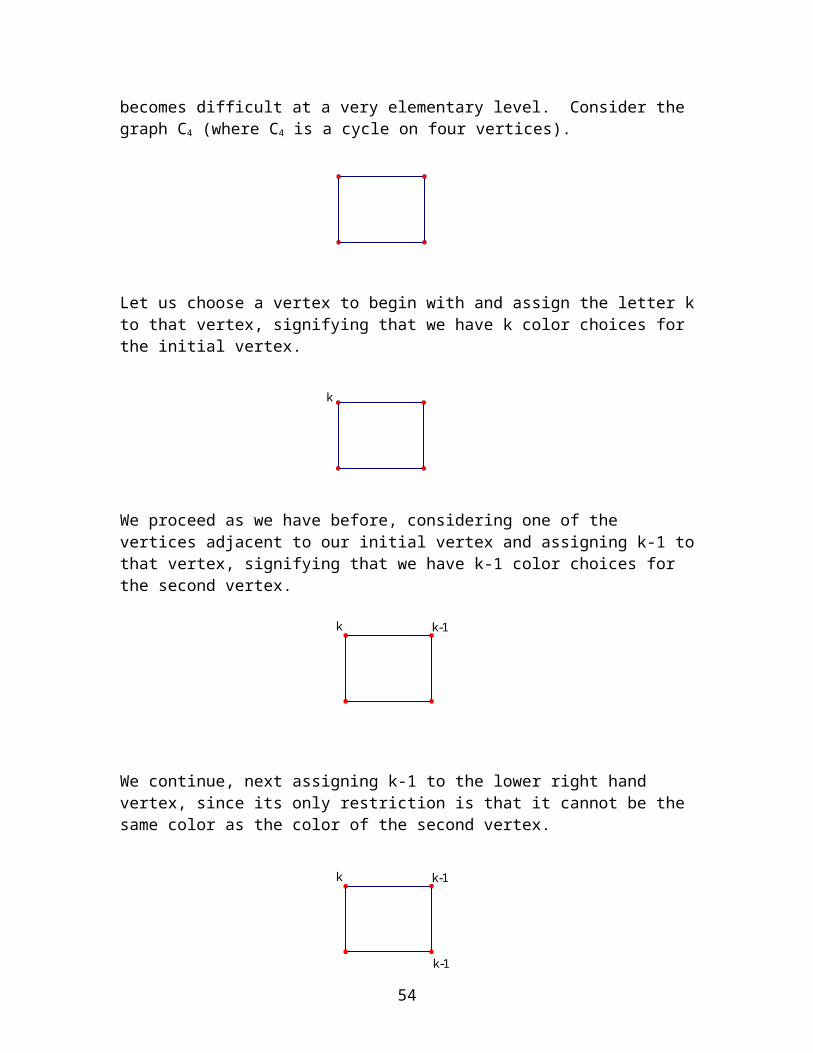
Are Chromatic Polynomials Always Easy to Find?Unfortunately the answer to this question is no. In fact, the task of finding the chromatic polynomial of a graph becomes difficult at a very elementary level. Consider the graph C4 (where C4 is a cycle on four vertices).
Let us choose a vertex to begin with and assign the letter k to that vertex, signifying that we have k color choices for the initial vertex.
42
k

We proceed as we have before, considering one of the vertices adjacent to our initial vertex and assigning k-1 to that vertex, signifying that we have k-1 color choices for the second vertex.
We continue, next assigning k-1 to the lower right hand vertex, since its only restriction is that it cannot be the same color as the color of the second vertex.
We now come to our fourth and final vertex and we are left with a dilemma. At first glance it may seem as though we very clearly have k-2 color choices for this last vertex, since it cannot have the same color as either of its two neighbors. However, there is nothing that says that the first and third vertex (the upper left and the lower right respectively) cannot have the same color. While they have a different number of color choices, their actual color could be the same or they could be different. If they are the same color, then our last vertex actually has k-1 choices. If they are different colors then our last vertex has k-2 choices, since it cannot be the color of either of its neighbors.
So how do we deal with this situation? We could use the addition rule of probability and sum the two separate cases. The graph on the left below is case one, where the upper left and lower right vertices have the same color. The graph on the right below is case two, where the upper left and lower right vertices have different colors.
This gives us:
(C4;k) = k(k-1)2 + k(k-1)(k-2)2 = k4-4k3+6k2-3k
43
k k-1
k k-1
k-1
+
k k-1
k-1 1 k-2k-2
k-1k

As you can see, carefully considering these special situations is time intensive, even at a rather simple level. The graph C4 only has four vertices in it. Imagine a large graph with multiple copies of C4 in it!
Deletion/ContractionA very powerful theorem helps us break down larger graphs into more manageable ones.For any edge e in G, let G-e be the graph formed by deleting e and let Ge be the graph formed by contracting e. Then we have the following:
Deletion/Contraction Theorem: (G;k) = (G-e;k) - (Ge;k)
In words, this says that the chromatic polynomial of G is equal to the chromatic polynomial of G with an edge deleted minus the chromatic polynomial of G with that same edge contracted. The letter e stands for an arbitrary edge, which means we can choose any edge we want to delete and contract.
So how does this help us? Note that both G-e and Ge are smaller graphs than G. The former is a graph with one fewer edge. The latter is a graph with one fewer vertex and one fewer edge. Thus, we can iterate this process, choosing a new edge each time to delete and contract until we are left with multiple smaller graphs for which we feel comfortable finding the chromatic polynomial.
To illustrate this process, let us take another look at C4. One of the edges below is labeled e, indicating that we will be deleting and contracting this edge. Doing so will produce two smaller graphs, also seen below.
The above notation seems to imply that the first graph is equal to the difference of the second two graphs. However, what we are really indicating with this schematic is that the chromatic polynomial of the first graph, C4, is equal to the difference of the chromatic polynomials of the second two graphs. The chromatic polynomials of the second two graphs are seen below, having been found using the conventional method we used earlier.
Thus,
44
e
G eG - eG
-=
-=
k-1k-1
k-1k k
k-2 k-1

(C4;k) = k(k-1)3 – k(k-1)(k-2) = k(k-1)((k-1)2-(k-2)) = k4-4k3+6k2-3k
Note that this checks with the chromatic polynomial on page 42.
A note to the teacher: I have included the following proof of the Deletion/Contraction Theorem for your benefit. If you feel as though your students would find the proof of this theorem beneficial, please feel free to share it with them.
Proof of Deletion/Contraction Theorem: Consider any two vertices in a graph A that are non-adjacent. Call them x and y. We have two cases to consider: either x and y have different colors or they have the same color. Thus, the total number of colorings of A will be equal to the total number of colorings of A where x and y DO NOT have the same color plus the total number of colorings of A where x and y DO have the same color.
Let us consider each case.
Case 1: x and y do not have the same color. If this is the case, then we can add an edge between x and y and not change the number of proper colorings of the graph A.Case 2: x and y do have the same color. If this is the case, then we can contract the two vertices into one, leaving one less vertex yet keeping the same number of edges that were present before. Call this contracted vertex z. Thus, if the deg(x) = m and deg(y) = n, then the deg(z) = m+n. Note that contracting two vertices into one vertex does not change the number of proper colorings of A.
As we stated above, the total number of proper colorings of A is equal to the total number of proper colorings in case 1 plus the total number of proper colorings in case 2. Graphically,
(Again, the above notation seems to imply that the first graph is equal to the sum of the second two graphs. However, what we are really stating is that the chromatic polynomial of the first graph is equal to the sum of the chromatic polynomials of the second two graphs.)
This being true, we can now subtract the second graph from both sides and be left with the following.
45
CB
+=
A
x y yx z

Hence, the total number of proper colorings of the graph B is equal to the total number of proper colorings of the graph A minus the total number of proper colorings of graph C. In symbols,
(B;k) = (A;k) - (C;k)
Note that A= B-e and C= Be
In other words,(B;k) = (B-e;k) - (Be;k)
A note to the teacher: The following activity brings nice closure to section 2.2, as it allows the students to witness the power of the Deletion/Contraction Method.
46
e
CA
-=
B
x y yx z

Activity: Deletion/Contraction Method Put to Use
Earlier, you computed the chromatic polynomial of different graphs without the use of Deletion/Contraction. Now do so using this very powerful technique. (Feel free to do so on a separate piece of paper – you will probably need one to draw and redraw each graph as you delete and contract).
47
DC
BA

Section 2.3 - Eulerian Circuits and Minimum Distance Spanning Trees
A note to the teacher: Unlike section 2.2, when a “warm-up” was included to refresh the students’ minds of the ideas presented in section 2.1, this section begins with a shift to a new topic.
To begin this section, students will be asked to analyze three different scenarios successively. In doing so, the hope is that the students will independently conclude the following:
1) Solutions to the scenarios are aided by an inspection of the corresponding graph.2) The number of edges “coming into” each vertex in the corresponding graph
determines the solution to the scenario.
I suggest the following strategy for the presentation of these three different activities: Introduce the first activity (The Bridges of Koenigsberg) and allow the students to work on it until you sense progress has ceased. It is likely your students will not independently make the two conclusions above after this first activity. That is okay – leave your students wondering as you move onto the second activity (Clearing the Streets of Treeville). They will be almost instantly successful with this activity (you will understand why soon). Once they have successfully completed this second activity, start them on the third activity (Clearing the Streets of Treeville – Part 2). The contrast between activities two and three should assist your students in making some conclusions about the nature of what is happening. This will allow them to return to the first activity armed with the tools necessary to make conclusions. This technique of leaving the first activity initially unresolved adds to the richness of your students’ subsequent discoveries.
48

Activity: The Bridges of KoenigsbergThe city of Koenigsberg (formerly of Germany, now part of Russia) consists of two islands and two banks of the Pregel River (the upper bank and the lower bank). Between these four land masses exist seven bridges, as seen in the map below.
The Koenigsberg Bridge Problem was a famous problem first posed and solved by Leonhard Euler in 1736 and is stated as follows: Is there a way that someone living on any of the four land masses can leave his or her home, walk across every bridge in the city exactly once and return to his or her home?
With a partner, explore this problem and come to a determination about whether or not such a route exists. Consider the following questions:
1) Does the location of the person’s home make a difference?2) Is there logical evidence to support your conclusion to the original question?3) Is there a way to model this situation using graph theory?
49

Clearing the Streets of Treeville
Welcome to the town of Treeville. Treeville is a small, rectangular town with only a few streets. Unfortunately, Treeville experiences a lot of snow and only has the money for one snowplow. The snowplow is kept in a garage at the corner of Elm and Cherry (vertex “A”). The folks of Treeville are undergoing a major financial crisis and need help determining whether they can route the snowplow in such a way that the snowplow does not traverse any street twice (the snowplow has to wind up back at the garage). Doing so would save on operational costs of the snowplow. Help the citizens of Treeville by determining whether such a route exists.
50
Oak
Evergreen
Fir
PineElm
Cherry
DogwoodBirch
Spruce
Dogwood
CactusApple
Cedar
Maple
Juniper
Redwood
A

Clearing the Streets of Treeville – Part 2
An attentive citizen of Treeville has brought to the attention of City Hall that one of the city’s street names needs to be changed. This mindful citizen has correctly noted that Cactus Street cannot be a street name in Treeville since a cactus is a bush, not a tree. The City Council strikes immediately, shutting down Cactus Street until another name can be thought of for this street (currently City Council has run out of tree names). The people of Treeville subsequently notice that the route you chose for the snowplow before no longer works. Can you find a new route that traverses every street exactly once? The new city map looks like this:
What frustrations, if any, are you having? What observations can you make?
How is this scenario different than the last one? Does this difference impact the ability to find a desired route? Why or why not?
51
Oak
Evergreen
Fir
PineElm
Cherry
DogwoodBirch
Spruce
Dogwood
Apple
Cedar
Maple
Juniper
Redwood
A

A few new ideas may help in determining solutions to the previous three activities.
26) Even vertex – a vertex v is an even vertex if the deg(v) is even27) Odd vertex – a vertex v is an odd vertex if the deg(v) is odd
In the graph G below, vertices a, b, c, and d are all even vertices and vertices e and f are odd vertices.
28) Even graph – a graph G is an even graph if EVERY vertex in G is an even vertex
29) Odd graph – a graph G is an odd graph if EVERY vertex in G is an odd vertex
Note that the graph G above is neither even nor odd, since some vertices in G are even and others are odd.
30) Circuit – a closed trail is a circuit when we do not specify the first vertex but keep the list in cyclic order. Circuits do not repeat edges but they can repeat vertices.
In the graph above, the closed trail a,b,e,c,d,e,a is a circuit. Note that edge ad is not in the circuit and thus not all edges are necessarily traversed in a circuit.
52
G a
e
d
c
b
f
a
d c
e
b

31) Eulerian circuit – an Eulerian circuit in a graph G is a circuit containing all of the edges. Remember, a circuit cannot repeat edges but can repeat vertices.
Note that the difference between a circuit and an Eulerian circuit is that a circuit is not required to contain every edge of G, whereas an Eulerian circuit is.
Eulerian circuits are named for Euler, who solved the Koenigsberg Bridge Problem by coming to the following conclusion:
Theorem: A graph G has an Eulerian circuit if and only if G is an even graph and all the edges of G lie in exactly one component.
Proof: (West, 2001, pp.27-28) Suppose G has an Eulerian circuit C. Since every passage through a vertex uses two incident edges (one that takes you into the vertex and one that takes you back out of the vertex), and the first and last edges of C are paired at the initial/ending vertex, then every vertex has even degree. Furthermore, two edges can be in the same trail only if they lie in the same component. Thus, if G has an Eulerian circuit C, then all of the edges of G must lie in exactly one component.
Now suppose that G is an even graph and all the edges of G lie in exactly one component. We will prove that G has an Eulerian circuit by induction on the number of edges, m.
Claim: (we need this for the proof below) If every vertex of a graph G has degree at least 2, then G contains a cycle.Proof of Claim: Let P be a maximal path in G and let u be an endpoint of P. Since P cannot be extended, then every neighbor of u must be a vertex of P. Since u has degree at least 2, then it must have a neighbor v that is also a vertex in P and the edge between them (uv) must be an edge NOT in P. Thus, the edge uv completes a cycle with the portion of P from v to u.
Base case: Let m = 0. If there are no edges in G, then a closed trail consisting of a single vertex suffices.
Induction Step: Assume true for graphs with < m edges. In the nontrivial component of G (the component with one or more edges, and thus all m edges), each vertex must have degree at least two. By claim above, this nontrivial component has a cycle. Call this cycle C. Let G’ be the graph obtained by deleting the edges of C from G. Since every vertex of C has two edges, the resulting components of G’ also are even and have fewer than m edges. By induction, each component of G’ has an Eulerian circuit. Thus, to obtain an Eulerian circuit for G, we traverse the cycle C, but when a component of G’ is entered for the first time, we take a detour along the Eulerian circuit of that component. This Eulerian circuit ends at the same vertex it began. At that point, we continue along C
53
until the next component of G’ is reached. We continue this process until C and each component of G’ is traversed completely. This forms the Eulerian circuit of G.
Because Eulerian circuits are straightforward and have real-life applications, the topic is easily presented and understood. The bi-conditional nature of the theorem allows us to quickly determine whether a graph contains an Eulerian circuit.
From the activities presented, it is already evident that Eulerian circuits are useful in routing situations. For instance, Eulerian circuits are sought in connection to the deployment of street cleaners, postal carriers, and buses, just to name a few.
Spanning Trees and the Shortest Distance AlgorithmWe have been focusing on graphs that have cycles. Now we will once again shift gears and turn our attention to a special family of graphs that do not have any cycles – trees.
32) Tree – a tree is a connected graph that contains no cycles
A few examples of trees are shown below.
54
CBA

Activity: The Chromatic Polynomial of Trees
In section 2.2 we found chromatic polynomials to be powerful in determining the number of proper colorings for any specified graph. Can you determine the chromatic polynomial of a tree with n vertices? Furthermore, can you determine the number of edges of a tree with n vertices?
55

A special kind of tree is called a spanning tree.
33) Spanning tree – a spanning tree of a graph G is a connected subgraph H with no cycles that “reaches” every vertex. By that we mean that every vertex of G is in our subgraph H
An example is in store. The subgraph H below is a spanning tree of the graph G below.
It is important to note that graphs often have multiple spanning trees. There is an enormous number of spanning trees contained in the graph G above.
Before taking a look at a spanning tree of interest in real-life applications, we must introduce one more idea.
34) Weighted graph – a weighted graph is a graph whose edges have been given “weight” to represent the quantity of a specified characteristic.
To this point, our edges have either been unlabeled or labeled by letters. In modeling a real-life situation it is often helpful to assign numbers to the respective edges of a graph. These numbers could represent any number of things. For instance, a graph that models the adjacency of US states (as we saw previously) may have the vertices represent the respective capitals of those states. Thus, the labels on the edges could be representative of the number of miles between any two state capitals of bordering states.
Minimum Distance Spanning Trees
To determine the minimum distance spanning tree T from vertex x, we consider the weighted graph G and build a minimum distance spanning tree from the vertex x.
We consider the vertices adjacent to x and add the edge that is “cheapest”, and in doing so we add a vertex (call it y). We then consider only the vertices adjacent to x or y and add the next edge based on which edge gives us the “cheapest” route back to x given the edges we already have. After an edge is added (with its corresponding weight) along with the new vertex (say z), we continue this process until all vertices have been reached.
56
HG

This algorithm will produce the minimum distance spanning tree T of the graph G relative to the vertex x.
To highlight this process, we will find the minimum distance spanning tree of the graph G below.
We start with vertex x and consider the vertices adjacent to x (vertices a, b, and c). We compute the shortest distance back to x from each of these three vertices. Doing so reveals that it would take a weight of 7 from vertex a, 2 from vertex b, and 5 from vertex c. Thus, we choose vertex b and add to x the new vertex b and the edge in between x and b. We label this new edge with its weight.
We now consider all vertices adjacent to either x or b (vertices a and c). We again compute the shortest distance back to x from each of these two vertices with the restriction that the computations can only take into account existing edges (of which there is now one) and one “new” edge. Doing so reveals that the shortest way back to x from a would be a total of 6 (4+2) and that the shortest way back from vertex c would be 5. Hence, we choose vertex c and add to the existing tree the new vertex c and the edge cx.
57
2
x
b
9
75
7
54
4
5
4
2
6
Gx
a c
df
b
e
2 5
x
b c

We continue this process, now considering all of the vertices adjacent to x, b, or c (which are vertices a, e and f). We compute the shortest distance back to x from each of these using the existing tree and one new edge. From vertex a the shortest distance back to vertex x is a total of 6, from vertex e the shortest distance back to vertex x is a total of 10, and from vertex f the shortest distance back to vertex x is a total of 12. Hence, we choose vertex a and add to the existing tree the new vertex a and the edge ab.
We next consider the vertices adjacent to x, a, b, or c (which are the remaining three vertices: d, e, and f). From vertex d, the shortest distance back to vertex x is a total of 15, from vertex e the shortest distance back to vertex x is a total of 10, and from vertex f the shortest distance back to vertex x is a total of 12. Hence, we choose vertex e and add to the existing tree the new vertex e and the edge ec.
We are almost done – only two more vertices to “reach”. We next consider the vertices adjacent to x, a, b, c, or e (which are vertices d and f). From vertex d, the shortest distance back to vertex x is now a total of 14, due to the new edge that was added last time from vertex e to vertex c. From vertex f the shortest distance back to vertex x is still a total of 12. Hence, we choose vertex f and add to the existing tree the new vertex f and the edge fc.
58
2 5
4
x
b ca
2 5
4
5
x
b ca
e
2 5
4
5 7
x
b ca
e f

With only one vertex left to “reach”, we know we will add vertex d next. However, we must consider the quickest way back to vertex x from vertex d. Adding edge de allows us to get back to vertex x in a distance of 14. Adding edge da allows us to get back to vertex x in a distance of 16. Hence, we add to the existing tree the new vertex d and the edge de.
The tree T we have constructed is the minimum distance spanning tree from vertex x for the original graph G. Thus, the tree T shows the quickest or cheapest way to get from vertex x to any other vertex in the graph.
In this algorithm, there may be times when two or more vertices “tie” in terms of having the smallest weight back to the original vertex. In case of ties, it does not matter which vertex is chosen. The resulting tree will still be a minimum distance spanning tree. Keep that in mind as you work through the next activity.
59
2 5
4
5 74
Tx
b ca
e fd

Activity – Minimum Distance Spanning Tree
Use the algorithm just described to produce the minimum distance spanning tree relative to the vertex x of the graph below. Be sure to go through step by step, showing your work as you go.
60

How Are Minimum Distance Spanning Trees Helpful?
The minimum distance algorithm described above is a powerful tool that is used in a variety of different ways. For instance, fire stations can use this algorithm to find the quickest route from the fire station to any destination in the area that station serves. Paramedics can do the same. This algorithm can also be used by internet sites that provide map services to the user (i.e. the user is provided with the quickest route from a location of origin to a selected destination).
In the city of Portland, Tri-Met has installed Trip Planners along the bus routes in hopes of making the system more user-friendly. Riders are able to enter their current location and their intended destination and the Trip Planner prints out directions specifying the quickest route between those two points. To do so, the Trip Planner uses a minimum distance algorithm.
A note to the teacher: The concluding discussion with my test group centered on Portland’s Tri-Met Bus System and the applications of graph theory to the system. This served as a nice closing to our time together, as it gave us an opportunity to see some of the topics we had discussed being used in a familiar real-life application. Trees, minimum distance spanning trees, and cycles were among the topics specifically addressed.
For a complete description of the problem addressed, please see Appendix 1.
Please note that unlike the rest of this curriculum, this portion is not activity-based. Instead, it is an example of graph theory’s applicability to real-life situations.
61

Chapter 3
My Experience Using the Curriculum
Section 3.1 - Test Group
I used this curriculum with a group of thirteen of my former pre-calculus students at Portland State. I had taught each of them Trigonometry in either the fall or winter quarter of the 2001-2002 school year. When the curriculum was tested (spring quarter of 2002), most of them had either taken the first term of calculus or were in the process of doing so.
The advantage of testing this curriculum out on former students is that they all knew me and for the most part, they knew each other. This was beneficial for many reasons.
First, the curriculum is designed with group work in mind and with an emphasis on group problem solving. Because of this, students need to feel comfortable sharing with one another and with me. Remember, group problem solving can be a frightening experience, particularly for younger students. There are numerous external pressures that may inhibit productive problem solving – fear of rejection by peers, fear of reaching an incorrect conclusion, and the fear of trusting others in the group, just to name a few. Because many of the students knew each other we were able to comfortably begin right away with the group work.
Second, it was important to me to receive feedback about the course in hopes of improving it for the future and so that I could include some reflection within this project. As an instructor, I require my students to give me regular feedback in the form of a weekly email. I respond to each email and the subsequent open communication that takes place helps facilitate a more comfortable, productive learning environment. Thus, I knew that my former students would be willing to give me honest, open feedback because they had done so in the past and they had seen it implemented. This alleviated the potential difficulty of having students who did not know me well and might find it difficult to be open and honest with me.
Furthermore, the students who took part in this project had no true external rewards. No credit was received and no payment was made. Each student was asked to participate based solely on their ability to communicate and their desire to learn. Also, it is important to note that while many of these students had earned high marks in my Trigonometry course, not all of them did, nor were they chosen because of their academic achievement in that course.
The seminar was presented over the course of three sessions, each lasting from two and a half to three hours. Due to the length of each session, I designed each lesson in hopes of keeping the students active and engaged. Some lecture was needed so that everyone in
62

the group was working from the same definitions and understanding of key ideas in graph theory, but for the most part, students came to an understanding of the key concepts and ideas by “getting their hands dirty”. Exploration problems were posed and the discussions that followed were the birthplace of most of the key concepts and ideas that were learned.
63

Section 3.2 – My Analysis of the Experience
Before reporting what the students’ assessment of the experience was, I thought it important to include my own analysis. In the “Specific Comments” section, I include pointers on what confusions arose in the implementation of the curriculum as well as suggestions of how to deal with these confusions. The “General Comments” section discusses less content-focused issues.
Specific Comments on the Curriculum
Section 1 – Introduction to Graph Theory with a Focus on Graph Coloring
One of the biggest confusions from section 1 arose in regards to the US map coloring activity found on page 24. Numerous students were confused as to what the circles (or vertices) represented. When asked to properly color the map, many students began coloring in the regions between the vertices, thinking these regions represented different states. In actuality, the vertices represent different states and a line between two vertices represent an existing border between those two states. Be sure to address this when the activity is distributed to the students.
The last activity in the section (found on page 27) asks the students to model a real-life situation (final exam scheduling) with a graph. As I mention in my note to the teacher on page 28, students often misrepresent the problem by having the vertices represent people instead of classes. I believe this is a healthy process that is worth going through – they may come to a correct conclusion by themselves! But if not, be prepared to gently guide them down the right path.
Section 2 – The Chromatic Polynomial
As I have mentioned previously, this section was the most difficult for the students. The biggest challenge for them was to understand that the letter k did not represent a color, but rather the number of color OPTIONS available to color each vertex. For example, students repeatedly got hung up on two adjacent vertices both being labeled k-1, because they knew from the first section that a proper coloring requires adjacent vertices to have different colors. However, as we learned in this second section, k-1 merely stands for the number of color options available for each of these vertices. I plan to be more clear about this distinction in the future when I teach this material.
Also, there was some confusion over the difference between k and K. It is important to note that k stands for the number of color options available to color a vertex, while K (followed by an integer) stands for a complete graph.
Finally, the deletion/contraction method is more easily understood with practice. My experience is that students feel more and more comfortable with the result once they have
64

implemented it themselves on a few graphs. Thus, be sure to take the time to have the students gain some experience with the method.
Section 3 – Eulerian Circuits and Minimum Distance Spanning Trees
This third and final section was pretty straightforward. The only comment I have regards the minimum distance spanning algorithm and is similar to the comment I made about the deletion/contraction method. I found that the students did not completely understand what was happening until they had the opportunity to wrestle with the algorithm a little bit themselves. Again, allowing time for them to construct minimum distance spanning trees themselves proved fruitful.
General Comments on the Curriculum
1) Working in pairs/groups
The format of the seminar was such that students were encouraged to work in pairs or groups on most problems/activities. This seemed to work well, as it gave them an opportunity to bounce ideas off of each other. Since the material was new to them, most problems were not easily solved using previous knowledge. In other words, some thought process was necessary to tackle the problems at hand. The sharing of information and ideas helped facilitate this process. Furthermore, working in groups made it evident to the students that there is more than one way to solve a problem, an important lesson in problem solving.
2) Hands on activities
Many students commented to me throughout the seminar that they really enjoyed the opportunity to solve problems themselves instead of having me solve all of them in the course of a lecture. They reported feeling more involved in the learning process. As a result of their involvement, I believe the conclusions they reached and the discoveries they made will be more long lasting.
It was exciting to walk around the classroom and see the students enthusiastically debating the intricacies of a problem with one another. This type of interaction would not have happened had I stood at the front of the classroom and lectured the whole time.
3) Time issue – longer sessions allowed for fewer “refreshers”
Prior to the seminar, I was concerned about the duration of each session (three hours) being detrimental to the learning process. I was pleasantly surprised however that these long sessions allowed students to explore problems at greater depth without their thought processes needing to be interrupted due to time constraints. Also, fewer, lengthier
65

sessions instead of more numerous shorter sessions reduced the amount of “refreshing” we had to do.
I believe that varying the instructional style is vital for keeping the students engaged over the course of a three-hour session. This curriculum is designed accordingly. There are numerous activities mixed in among the more traditional, lecture-based instruction.
4) Content level of difficulty (chromatic polynomials/deletion-contraction)
I felt as though the level of difficulty of the content was appropriate for the students I was working with. They seemed to grasp most of the concepts quickly, though they did struggle slightly with the section on chromatic polynomials and the deletion/contraction method. This was anticipated however. After consulting with my project advisor, we decided to “push the limits” by attempting to cover this more advanced graph theory concept. Suggestions for a clearer instruction of this material are included in chapter 2 of this project.
In general, I think the content difficulty pushed the students to think critically, yet never left them feeling lost.
5) Class size
The small class size (thirteen students) made it much easier as an instructor to get around to each group and observe what problem solving strategies were being implemented. Furthermore, with only a few groups, there was plenty of time to share solution methods to various problems. The small class size made a discussion-oriented learning process easier to facilitate.
6) Curiosity for more
One of the most positive signs regarding the experience was the curiosity for more learning by some of the students. Because of the applicability of the subject, students felt a connection to their every-day lives. As a result, many of them expressed an interest in exploring other topics within graph theory.
66

Section 3.3 – Analysis of Student Evaluations
At the end of the third and final session, I handed out an evaluation form to each of the students in the seminar. To ensure complete responses, I asked them to email me their responses at their convenience. Below is a copy of the evaluation form.
Evaluations of Experience
First off, let me again thank you for being willing to participate in this experience. I hope you’ve found it worthwhile, instructive, and enjoyable.
In hopes of gaining feedback, I would really appreciate your HONEST response to the following questions. If you would prefer, please feel free to email me your responses to these questions at [email protected]. Please be as specific as possible. Thanks!
1) What did you like best about this seminar?2) What could be improved (structurally or content-wise)?3) Did you at any time use skills you have learned in Calculus to deal with any of the
problems presented? If so, what skills were utilized?4) What did you learn about the way in which you solve problems? What factors
affect how you solve problems?5) Was the journaling of problem solving strategies/processes insightful? 6) What was your motivation for agreeing to take this seminar?7) Do you think this is a course that should be offered as an elective to the general
PSU student population (for those that have not yet had Calculus)? Why or why not?
Thank you for taking the time to give me honest feedback. I appreciate it!
I received feedback from 10 of the 13 students that were in the seminar. Their full responses are included in the appendix.
Analysis of Evaluations
The introduction of this graph theory curriculum was due largely in part to the hypothesis that pre-calculus skills are sufficient for a solid understanding of graph theory. With this in mind, I included question three above. The responses were almost completely unanimous in support of this hypothesis. Those that reported having used ideas they had learned in calculus focused their attention on the sigma notation they used in the solution of a single activity. It is important to note that the use of sigma notation was unnecessary for that activity.
“…the only piece of calculus knowledge I used (which I don’t think we even needed) was sigma notation for the chromatic polynomials.”
67

“…I have never taken a Calculus class. Obviously, Calculus skills are not needed to understand Graph Theory, because I understood it with relative ease.”
When asked if an introductory graph theory course should be offered as an elective to Portland State University students, all participants answered unanimously in the affirmative.
“I think that Graph Theory would be awesome as an elective math course because it would give people who are not mathematically inclined the chance to really visualize mathematics. This could be very useful to these people because, in understanding how easy it can be, it could change the way they think about math, or it could transform the way people discourage themselves from math by telling themselves they are bad at it. Graph Theory presents math in a different light, and I think that everyone could benefit from this perspective.”
“I definitely think this class could be taught and should be taught as a general elective without needing calculus. I was totally comfortable with the material, and…I think it would be a helpful class to have under my belt…It is a really good class to practice how to think through math concepts.”
An important part the evaluation process is hearing what students think could be improved. Answers varied in this regard. The following suggestions were made:
More practice problems or homework: A couple of students felt that they would have been able to solidify concepts better had they been given more opportunity to wrestle with the material.
I agree with this assessment. In a regular class format, homework would certainly be a viable option, whereas I was unable to assign homework due to the volunteer status of the participants. Again, I think the key to this curriculum is the students’ involvement in the problem solving process. Hence, the more opportunities the students have to get their hands dirty, the better. Homework would allow students to struggle with problems in depth, leading to more significant discoveries.
Use of more manipulatives: A few students praised graph theory for its visual approach to mathematics. With this in mind, they felt as though more manipulatives could be used in conjunction with some of the activities and that doing so would bring some of those activities more to life.
As has been mentioned previously, the goal of the curriculum is to get students involved. Bringing the problems to life is a great way to do this. Thus, any manipulatives that are appropriate to the problem solving situation are encouraged. For instance, the handshaking problem is a great way to bring the activity found on page 17 to life. Other ideas include using local street maps for the Eulerian circuit and minimum distance spanning tree problems instead of fabricated street maps.
68

Lengthen course into a regular ten-week course: Clearly this is the intention of the project. A lengthier course would allow students to study the main ideas of graph theory at a greater depth, as well as get glimpses of more advanced aspects of graph theory.
This last suggestion above is noteworthy for another reason. More class time would allow for the development of proof writing skills, an important set of skills to have before advancing to higher levels of mathematics. Furthermore, such an introductory course provides a convenient home for the development of two important themes in mathematics that often are discarded due to a lack of instructional time – problem solving and math modeling. In this curriculum, emphasis is placed on an acknowledgement by the students of the problem solving skills that are being used. As time allows, students can be encouraged to keep a problem solving journal that outlines the strategies they are using as they solve problems throughout the course. Periodic discussion of such heuristics may help students with their problem solving skills.
69

Chapter 4
Additional Comments
Section 4.1 – Other Topics
For those teachers interested in teaching a lengthier course in introductory graph theory, I include now a list of other graph theory topics. These topics extend beyond the curriculum constructed in this project, but could be easily incorporated with this course and would be very appropriate topics for newcomers to graph theory.
- Bipartite Graphs- Isomorphic Graphs- Directed Graphs- Network Flow - Hamiltonian Cycles
Each of these topics is discussed at some depth in most textbooks (see Section 4.2 - Suggested Textbooks).
70

Section 4.2 – Suggested Textbooks
The following is a short, and by no means comprehensive, list of suggested graph theory textbooks, with a brief description of each. Please see the references for source information.
1) Introductory Graph Theory by Gary Chartrand
This book is an introductory text that is easy to read and understand. One of the author’s stated objectives is “…to show how graphs are applicable to a wide variety of subjects, both within and outside mathematics.” (http://www.wmich.edu/~mathstat/people/faculty/chartrand/introgt/AboutBook.html)
It covers a variety of topics including: basic properties of graphs, Eulerian circuits, trees, and graph coloring. One advantage of this book is its cost – around $10.
2) A First Look at Graph Theory by John Clark and Derek Allan Holton
This book is an introductory text that is intended for mathematics students with little or no background in graph theory. Topics covered in the book include: a general introduction to graphs, tress, connectivity, Eulerian circuits, planar graphs, graph coloring, and directed graphs. The book places a heavy emphasis on algorithms and applications.
3) Pearls in Graph Theory by Hartsfield and Ringel
This book is an easy to read, entertaining text that covers the major topics in graph theory. No previous experience with graph theory is needed though the book does cover the material in depth and includes challenging problems for all students. This book has been revised and new activities and problems have been added based on advice from educators who have used the previous edition.
4) Introduction to Graph Theory (2 nd edition) by Douglas B. West
This book is a text designed for use at the undergraduate or advanced graduate level. No previous knowledge of graph theory is assumed. Topics covered in the text include: fundamental concepts of graphs, trees, graph coloring, and planar graphs. This book also includes more advanced topics like matroids and eigenvalues.
5) Online Tutorial by Chris Caldwell
Finally, I have also included the following link to a great online tutorial in introductory Graph Theory. The tutorial covers many of the same topics covered in the curriculum I have created. This site also provides links to other online resources in Graph Theory.
71

http://www.utm.edu/departments/math/graph/
72

Appendix 1
Improving Portland’s Tri-Met Bus System
Current System
Portland is serviced by approximately one hundred different bus lines. The current routing scheme is that of a hub-and-spoke system, similar to the system the major airlines use. Downtown Portland’s shopping and business district serves as the central hub, with spokes exiting in various directions to service the other parts of the city. These spokes connect the central hub to regional hubs, which in turn have spokes exiting them to service each of the local areas. Some regional hubs include Beaverton, Hillsboro, Gateway, Clackamas, Oregon City, Gresham, Vancouver, and Washington Square. Figure 1 below shows a rough illustration of the network.
From a graph theorist’s perspective, Portland’s current bus system is interesting in that there are no major circuits in the system. To be sure, the route of each bus is a loop, but with few exceptions, each bus returns along the same streets it traveled in the outgoing direction. However, there are no direct loops around the perimeter of the city, for example. It is evident that the central hub has been given precedence in the construction of this system, with hopes of minimizing travel from the central hub to any vertex (bus stop) in the system.
This “shortest distance” approach for downtown is beneficial in terms of servicing riders wanting to come into downtown or leave downtown to reach other parts of the city. However, customers who have no need to reach downtown but must travel between regional hubs are penalized greatly. For instance, imagine Mrs. X lives in Oregon City but works in Beaverton. Currently there are no direct connections between these two regional hubs. Thus, if Mrs. X wants to use Tri-Met, she must travel into downtown and back out to Beaverton. According to Metro, this trip takes about twenty-six minutes by car (traveling directly between Oregon City and Beaverton). Yet by Tri-Met the same trip takes over eighty minutes, over three times as long as it takes by car. The choice is
73
Figure 1
Portland
Vancouver
Gateway Gresham
Clackamas
Oregon City
Beaverton
Washington Square
Hillsboro

an easy one to make for Mrs. X. Hence, another person drives a car instead of taking the bus.
This poor ratio in travel time is something that Tri-Met must minimize if it wants to increase ridership and as a result, reduce traffic congestion in the system.
A Little BackgroundIn September of 2001, I stumbled upon a government document entitled The State of the Art in the Routing and Scheduling of Vehicles and Crews. This report had been put together by researchers at the University of Maryland under the leadership of Lawrence Bodin, Bruce Golden, Arjang Assad, and Michael Ball. This comprehensive report looked at various computational strategies and algorithms for solving scheduling and routing problems common among municipalities. The hope was to provide cities with a tool with which they could “counteract the rising costs of moving goods and people from place to place.” (Bodin, 1981, abstract)
Impressed by how thorough the report was, I began to wonder if all municipalities were following such strategies when setting up a transportation system. My hunch was that most organizations were not fortunate enough to have a discrete mathematician/graph theorist in their midst. Furthermore, I suspected that most organizations had not even seen such a comprehensive document.
In hopes of gathering some information regarding Portland’s system, I met with Ken Zetarin of Tri-Met in the fall of 2001. I shared the aforementioned document with him and asked him if there were any trained mathematicians working for the development team at Tri-Met. He mentioned that his mathematical training had included calculus and differential equations, but that most of his training for the position had been centered around urban planning. When asked if his development team used approaches outlined in the Department of Transportation document, he said that he was not aware of such a document and that most decisions in terms of system layout are made from a “common sense” perspective or from previous experience. He also mentioned that political conditions effect the decisions that are made regarding system layout.
I quickly gave a brief synopsis of my understanding of graph theory’s use in the routing and scheduling of buses and followed that by asking Ken where he thought such an approach could be used in addressing some of the current problems in the system. Many potential problems were discussed, with Ken patiently explaining to me how these problems had come about and why they needed to be addressed. One problem in particular caught my interest.
74

The ProblemAs I mentioned previously, Portland’s Metro system is a hub and spoke system, with efficiency defined as service to the downtown area. This creates a problem though when people want to travel between spokes in the system. In hopes of increasing ridership and better serving their patrons, Metro was interested to know whether it made sense to connect any of the regional hubs directly, and if so, which ones made the most sense to connect. Since cost is always an issue (and a limitation), the ultimate goal was to determine which regional hubs would serve the most people if connected.
I started by defining the regional hubs of interest – Beaverton, Clackamas, Gateway, Gresham, Hillsboro, Oregon City, and Washington Square. Vancouver is also considered a regional hub but I chose to simplify the problem by limiting my focus to the seven listed above. Vancouver is already being serviced by way of I-5 and I-205, since these are the only two ways of accessing Vancouver across the Columbia River. Since none of the other seven hubs were being served via the highway system, it made sense to focus on those. In other words, Vancouver is seemingly already being serviced in the most efficient manner.
Having defined the hubs, the next step was to gather information about the ridership between each of these hubs. I was most interested in weekday commuters who entered the system at one regional hub and exited it at another. Travel before and after entering or exiting at these hubs was unimportant to me, as it only would confuse the process. Remember, the focus of this project was to monitor travel between regional hubs, so what happened before and after the regional hubs did not need to be considered.
Metro breaks down the Portland area into 1020 zones. These zones vary in size, depending upon the population in each zone. Thankfully, Metro was able to provide me ridership data on travel taking place between any two of these 1020 zones. Actual mean ridership for a normal workday and potential mean ridership for a normal workday was provided.
By actual ridership, I mean the average number of people who “enter” the system at any given regional hub and then “exit” the system at another regional hub.
By potential ridership, I mean the number of people that travel between any two regional hubs on a normal workday for any purpose. Thus, not only are actual Tri-Met riders counted, other people using alternative modes of transportation (personal automobile, etc.) are counted as well. I was concerned with the validity of these numbers and so I pressed Scott Higgins of Metro on this issue. He assured me that extensive surveys had been done to determine the number of people that travel back and forth between any two zones in the system, regardless of the mode of transportation.
I was interested in four different pieces of information – total number of actual riders between any two zones, total number of potential riders between any two zones, average automobile trip time between any two zones, and average transit trip time between any
75

two zones. However, the resulting 1020 by 1020 matrices were a bit overwhelming to deal with so we decided to simplify things by aggregating the zones into seven main zones, centered about the regional hubs mentioned above. Higgins chose seven zones that host the transit centers at each of those seven regional hubs and then aggregated all zones within five minutes of each of those regional hubs. Thus, the matrix was reduced to a more manageable size of seven by seven.
Four seven by seven matrices were produced, covering the requested information above. Tables 1, 2, 3, and 4 are shown below.
Key for Tables
H = HillsboroB = BeavertonWS = Washington SquareOC = Oregon CityC = ClackamasGR = GreshamGA = Gateway
Table 1 – # of Actual Tri-Met Riders Between Hubs
H B WS OC C GR GAH 892 129 22 1 1 1 3B 129 1667 391 6 6 7 20WS 22 391 874 8 4 3 9OC 1 6 8 252 57 5 18C 1 6 4 57 783 34 157GR 1 7 3 5 34 888 102GA 3 20 9 18 157 102 1334
Table 2 – Total # of Commuters Between Hubs
H B WS OC C GR GAH 48206 2379 745 19 28 8 33B 2379 88282 25765 223 231 118 341WS 745 25765 63133 418 299 94 231OC 19 223 418 23410 5294 306 773C 28 231 299 5294 56476 1928 5621GR 8 118 94 306 1928 83729 4126GA 33 341 231 773 5621 4126 49027
76

Table 3 – Midday Auto Times (in minutes)
H B WS OC C GR GAH --- 18.2 24.0 43.7 47.8 54.1 39.8B 18.5 --- 7.4 27.1 31.7 38.3 24.0WS 24.1 7.1 --- 22.1 29.0 40.9 26.6OC 43.3 26.3 21.3 --- 10.0 28.2 19.5C 47.4 31.0 28.0 9.9 --- 22.3 13.5GR 52.8 37.6 39.8 28.5 22.3 --- 16.4GA 39.5 24.2 26.5 20.1 13.5 16.5 ---
Table 4 – Midday Tri-Met Transit Times (in-vehicle plus out-of-vehicle times – in minutes)
H B WS OC C GR GAH --- 37.9 56.7 103.3 102.9 102.7 83.0B 37.8 --- 23.4 75.6 75.2 75.0 55.3WS 65.4 32.0 --- 87.6 84.5 94.7 75.0OC 101.7 80.1 87.8 --- 38.2 99.0 76.6C 109.0 81.4 91.7 38.5 --- 61.8 42.1GR 103.1 75.5 95.9 96.1 63.6 --- 30.5GA 82.9 55.3 75.7 75.8 43.3 29.9 ---
Actual Riders versus Potential RidersThe numbers are alarming. On average, just 1.7% of the potential riders are using Tri-Met as their mode of transportation. What is particularly troublesome is the vast quantity of “lost” riders from the Beaverton/Washington Square hubs, an area of Portland suffering badly from congestion. It is staggering to consider the untapped potential that Tri-Met represents as a means of transportation. So why aren’t people choosing Tri-Met over their own automobiles? Time. Whether it be business men and women that work downtown or shoppers wanting to get across town to their favorite shopping mall, people want to be efficient with their time. We live in a society that favors efficiency and rejects waiting. So why would someone with a car choose to ride the bus if it takes them twice as long to reach their destination?
Transit Time versus Automobile TimeTables 3 and 4 show the average trip time between regional hubs in the system for Tri-Met and automobiles respectively. It is quickly evident that car travel is much quicker than bus travel. Clearly, a major reason for this is that buses must pull over every couple of blocks to pick up and drop off riders. In fact, Portland has the shortest “stop distance” of any city in the country, an issue that has come under considerable scrutiny in hopes of improving the system. But is “stop” time what is to be blamed for the huge discrepancy in travel times? Not entirely.
77

Compare for example the time it takes to travel from Oregon City to Beaverton by car and by bus. It takes a little over twenty-six minutes by car and over eighty minutes by bus. The fifty-four minutes of lost time have more to do with route than with stop time. While buses will never be as fast as cars (due to the requirements to unload and load passengers more frequently), there is much that can be done to close the gap between the two travel times.
What is the most efficient way for a car to travel between Oregon City and Beaverton? Drive into the heart of Portland and back out or use the interstate system that avoids the center of the city?
To more clearly express the difference in travel time between hubs, I computed the ratio of transit time over auto time. Table 5 below shows the results. Table 5 – Transit Times/Auto Times
H B WS OC C GR GAH --- 2.1 2.4 2.4 2.2 1.9 2.1B 2.1 --- 3.2 2.8 2.4 2.0 2.3WS 2.7 4.5 --- 4.0 2.9 2.3 2.8OC 2.4 3.0 4.1 --- 3.8 3.5 3.9C 2.3 2.6 3.3 3.9 --- 2.8 3.1GR 2.0 2.0 2.4 3.4 2.9 --- 1.9GA 2.1 2.3 2.9 3.8 3.2 1.8 ---
For the most part, the ratios were inversely proportional to the distance between hubs. This makes sense, as the effect of stop time is diminished over time.
Table 5 shows that the worst connections are Beaverton/Washington Square, Oregon City/Washington Square, and Oregon City/Clackamas.
We realized however, that some importance needed to be given to the total number of people we could potentially affect by adding a connection to the system. While Oregon City and Washington Square had one of the worst connections, they did not have the most potential riders commuting between them. Thus, it made sense to factor in potential ridership when determining the connections of highest priority. It is more rewarding financially to dramatically improve the system for the highest number of people.
With this in mind, a sixth matrix was computed, wherein a value was assigned to each pair of hubs based on the following importance function: # of potential riders * travel time ratio. Table 6 below shows us the Importance Matrix.
78

Table 6 – Importance Function (Rounded to nearest integer)
H B WS OC C GR GAH --- 4965 1760 45 60 15 69B 4874 --- 81519 623 547 231 785WS 2021 678 --- 1654 870 218 651OC 45 678 1726 --- 20335 1074 3039C 64 607 981 20619 --- 5343 17585GR 16 237 226 1031 5500 --- 7659GA 69 778 660 2923 18045 7488 ---
From this information, I then made a pairwise list of hubs from most important connection to least important connection.
1) Washington Square/Beaverton2) Clackamas/Oregon City3) Gateway/Clackamas4) Gresham/Gateway5) Gresham/Clackamas6) Hillsboro/Beaverton7) Oregon City/Gateway8) Washington Square/Hillsboro9) Washington Square/Oregon City10) Oregon City/Gresham11) Clackamas/Washington Square12) Beaverton/Gateway13) Washington Square/Gateway14) Oregon City/Beaverton15) Clackamas/Beaverton16) Gresham/Beaverton17) Gresham/Washington Square18) Gateway/Hillsboro19) Clackmas/Hillsboro20) Oregon City/Hillsboro21) Gresham/Hillsboro
Armed with a list of the most “costly” connections (in terms of “importance” defined above), I began analyzing the current system in regards to each of these connections.
1) Washington Square/Beaverton
Looking at the tri-met system map, we tried to figure out which bus route someone would most logically take to get between these two regional hubs. We determined that either the 76 or the 78 would be the most logical choice. We then discussed the difference between the route these two buses take and the route someone would take by car. The
79

buses take a more local route, which makes sense because they must pick up and drop off passengers along the way. This is a slow process though, particularly in the congested streets of Beaverton. Furthermore, the service of these local passengers is not what we are concerned with. Remember, we are interested in improving the travel of people that come into the system prior to one regional hub and exit the system after another regional hub. Thus, we do not care about patrons entering or exiting the system BETWEEN the hubs.
If someone were traveling by car, they would most likely take I-217. While it is true that I-217 is also congested, the traffic is more free flowing than local traffic is on the city streets (due to stop lights, etc.), and thus takes less time. Therefore, it makes sense to have a bus that uses this route. The addition of HOV lanes would allow the bus to travel more quickly between the two hubs, particularly if a left exit ramp were introduced that could be used by buses only (this would alleviate the issue of the bus needing to cross back over a lane of traffic to exit after the quick trip up (or down) I-217).
2) Clackamas/Oregon City
We followed the same process as before, looking first at the Tri-Met map to analyze the current route between these two regional hubs. Currently, the quickest route by bus between these two hubs is the 79. A close look at its route however reveals that the route is rather circuitous. That is evident by the poor ratio between transit time and auto time (on average it takes 3.9 times as long by bus as it does by car). Such a poor ratio suggests that the auto time is being achieved by another route, namingly the use of I-205. As is the case with the Washington Square/Beaverton connection, the current bus connecting the two hubs is required to make local stops in between to serve patrons in those areas. Once again, this slows the travel for the riders we are most interested in. An express bus that makes use of I-205 seems to make the most sense.
3) Gateway/Clackamas
The quickest route between these two regional hubs is by way of the 72, which travels north and south on 82nd Avenue. Geographically, this is a rather direct route. However, 82nd Avenue has a lot of stoplights and a lot of stop and go traffic. Furthermore, the 72 makes a stop every few blocks as it travels up and down 82nd Avenue. Stop time and traffic lights slow this connection considerably. Again, the poor ratio between transit time and auto time (3.2) suggests that cars are taking a more efficient route. I-205 is a much quicker means by which these two regional hubs can be connected, and with the use of HOV lanes, an express bus could be introduced that would greatly reduce the time it takes to travel between the two hubs.
Since the Oregon City/Clackamas and Gateway/Clackamas connections both could be improved by use of an express bus on I-205, it is logical to propose an express bus that travels back and forth between all three of these hubs (Gateway to Clackamas to Oregon City and back).
80

Generalizing to Arbitrary Weighted Graphs
It is difficult to argue downtown Portland’s place of importance in the system. And hence, it makes sense to use the minimum distance algorithm (refer to page 54) when setting up the system. However, as has been mentioned previously, the least distance algorithm is extremely efficient for coming and going from exactly ONE vertex. But what if more than one vertex in the graph is important? Is there a way to alter the algorithm slightly to make the system most efficient for two vertices? Or three vertices? Or n vertices?
We have discovered that due to the sheer number of people living in Washington County, there is a great potential for improving the flow in and out of the Washington Square and Beaverton hubs. So what if we made Beaverton and Washington Square our second and third vertices of importance and then arranged the system so that these two vertices were served second and third most efficiently?
In general terms, for a graph of n vertices, ordered in importance from 1 to n, with e allowable edges of total weight w, is there an algorithm that will provide the most efficient overall system? By most efficient overall system, we mean the following: Vertex 1 (vertex of highest importance) will have the least overall distance to the n-1 other vertices in the system, Vertex 2 (vertex of second highest importance) will have the second least overall distance to the n-1 other vertices in the system, and so on, all the way down to Vertex N (vertex of least importance), which will have the greatest overall distance to the n-1 other vertices in the system.
If there was such an algorithm, municipalities could rank their regional hubs in order of importance (though this in and of itself would be a practice in political warfare) and then lay out a system that would serve the greatest number of people in optimal efficiency.
The idea of such an algorithm fascinated me, so I decided to play around with some self-created graphs in hopes of finding some kind of pattern or approach to the problem.
I began with the complete graph on seven vertices, with the vertices spaced similarly in structure to the Portland central and regional hub system, with the Vancouver hub added and the Hillsboro and Gresham hubs deleted since they’re merely extensions of Beaverton and Gateway respectively. I then gave arbitrary weights to each of the twenty-one edges in the graph.
81

85
4
3
6
2
5
8
6
77
9
10
8
11 7
9
9
12
9
12
Complete Graph on 7 Vertices
A
B
C
D
E
F
G
Obviously, a complete graph would be optimal, with every hub in the system being directly connected to all the other hubs. However, this is not financially feasible, nor efficient. Thus, each municipality has certain financial restrictions on the number of bus lines they can have, and thus the number of direct connections they can have. With this in mind, I decided to put arbitrary restrictions on the problem.
1) Only 2/3 of the total possible number of edges would be allowed. Since I had 21 possible edges, only 14 of them would be allowed in the final graph.
2) Total weight of the system would be limited similarly. Based on the arbitrary weights I’d given each edge, the K7 system had a total weight of 157. 2/3 of 157 is approximately 104. Thus, the allowable weight in the system would be 104.
3) The vertices were prioritized arbitrarily as follows (from most important to least important): A, B, C, F, G, E, D
So the goal had been established: Create a system with 14 or fewer edges, maximum total weight of 104, and with highest priority given to vertex A and so forth on down to vertex D.
I was first interested to know if the direct connections between pairwise vertices were the most efficient routes between those specific vertices. If not, I would be able to potentially eliminate some edges right away for “free”. This will become more evident momentarily.
I ran the minimum distance algorithm on all pairwise vertices to determine the shortest path between any two vertices in the system. Table 7 shows the minimum distance matrix.
82

Table 7 – Minimum Distance
A B C D E F G TotalA -- 5 6 7 7 9 8 42B 5 -- 2 8 11 10 8 44C 6 2 -- 6 9 12 9 44D 7 8 6 -- 3 7 10 41E 7 11 9 3 -- 4 7 41F 9 10 12 7 4 -- 5 47G 8 8 9 10 7 5 -- 47
Using the minimum distance algorithm for each pair of vertices uncovered for me some interesting information. Some of my existing edges were unneeded, in that there were more efficient paths that avoided these edges, making the edges excess. Removing these edges would reduce the total number of edges in the system (getting us closer to our goal of 14) and the total weight in the system (which also would get us closer to our goal of 104).
Below is the graph of K7 – Unneeded edges.
85
4
3
6
2
5
8
6
77
9
10
79
Complete Graph - Unneeded Edges
A
B
C
D
E
F
G
Six edges turned out to be “unneeded” in this example, and those six edges combined to produce 61 units of total weight. Thus, our graph has now been reduced to a graph on seven vertices, with 15 edges and 96 units in weight. Our weight requirement has been met and we need only to cut one more edge to satisfy requirement #1. But what about the third requirement? Is the total weight from each vertex to the other vertices such that the vertices are in the required order of importance?
83

Below is a list of the vertices and the sums of the distances to the other six vertices. In parenthesis are the desired order.
D = 41 (7)E = 41 (6)A = 42 (1)B = 44 (2)C = 44 (3)F = 47 (4)G = 47 (5)
Our current graph clearly does not satisfy the third requirement. Vertices E and D are supposed to have the second greatest and greatest total weight respectively, yet currently they are tied for the least. With this in mind, something must be done to remove one final edge from the graph such that vertices D and E are penalized enough to put them at the end of the list for total weight.
Unfortunately, to remove such an edge so that the vertices are in the correct order, also requires us to worsen the overall system so badly that it is not worth it. For instance, if we were to remove edge DE, then the total weights for D and E would go up significantly. Just to get from D to E, one would need to travel through A (the central vertex) first, and then to E, for a total weight of 14. Thus, both D and E’s total weight would be increased by at least 11, which would help us in terms of our priority order (D and E would no longer have the least total distance). However, other vertices totals would be impacted as well. For instance, with edge DE in place, it takes a weight of 7 to get from F to D. But with edge DE removed, that total would go up to 16 (one would have to travel from F to A and THEN to D). Thus F’s total weight would increase significantly as well.
Based on the examples above, we can conclude that our goal of producing the most efficient system is complicated when we are forced to take vertices’ priority into account. To do so is costly in terms of keeping the total weight of the system minimal. Changes that are made to improve the order of the vertices are not worth the total weight that is added to the system.
Furthermore, in regards to an actual city, it is likely that the total weight for the central vertex (which most likely is deemed the vertex of highest priority) will exceed that of the other vertices. If we define “weight” to be the time it takes to travel between vertices, it is logical to assume that due to high traffic volumes within the center of a city, total weight will be impacted more greatly for the central vertex than any of the outlying vertices. Since it is likely that traffic will be more free-flowing outside of downtown, the total weights for the outlying vertices should be smaller. Thus, it may be impractical to set up a system that orders the vertices by way of priority.
84

What have we learned?Abstraction to graphs allows us to see potential improvements by adding circuits. It also allowed us the insight to understand the difficulties of trying to generalize the minimum distance spanning algorithm to satisfy a prioritization of vertices, as several illustrative counterexamples were readily produced. And in terms of bus routing, this exploration has shown us that high traffic flow in the center of a city makes it difficult to reduce the total weight of a bus system by taking away outer edges. To avoid this traffic, it makes the most sense to connect some of these regional hubs directly, as we discussed earlier. Outer edges will have less weight than central edges do, particularly when you begin to consider the use of highways and freeways.
As automobile use increased in the 1900’s, municipalities countered city congestion by building beltways designed to reroute traffic around the heart of the city. People that lived on one side of town that needed to travel to the other side of the city no longer had to fight slow traffic downtown. This simple solution worked so well that the majority of cities in the United States employ such a system for traffic. Surprisingly, the same idea is rarely used to route buses.
85

Appendix 2
Reference Sheet
This is a reference sheet that I think might be helpful to keep in your notes as we progress through this learning experience. I remember as I learned this stuff that it was at times difficult to recall the distinction between the different terms. Thus, this can serve as a “cheat sheet” of sorts.
1) Adjacent – two vertices are adjacent to one another if they are the endpoints for the same edge
2) Neighbors – two vertices are neighbors if they are adjacent to one another3) Isolated vertex – a vertex v is an isolated vertex if it has no neighbors4) Loop – a loop is an edge whose two endpoints are the same vertex5) Multiple edge – two edges that have the same endpoints are called multiple edges6) Simple graph – a graph is a simple graph if there are no loops and no multiple edges7) Walk – a walk is a sequence of vertices such that consecutive vertices are neighbors8) Closed walk – a closed walk is a walk that begins and ends at the same vertex9) Trail – a trail is a walk with no repeated edge10) Closed trail – a closed trail is a trail that begins and ends at the same vertex11) Path – a path is a walk with no repeated vertices12) Cycle – a cycle is a closed path (no repeated vertices other than the first and last)13) Subgraph – a subgraph H of a graph G is a graph whose edges and vertices are
subsets of the edges and vertices of G14) Connected – a graph is connected if for any two vertices u and v in the graph there
exists a path between those two vertices15) Component – a component of a graph is a maximally-connected subgraph16) Cut-vertex – a vertex v is a cut-vertex if removing v from the graph (and any edges
touching v) increases the number of components of the graph17) Clique – a clique (pronounced kleek) of size n is a collection of n vertices that are
pairwise adjacent (in other words, each of the n vertices is adjacent to the other n-1 vertices in the clique)
18) Degree of a vertex – the degree of a vertex v (denoted deg(v)) is the number of edges that have v as an endpoint
19) Complete graph – a complete graph on n vertices (denoted Kn) is a graph with n vertices that are pairwise adjacent (each of then vertices is adjacent to the other n-1 vertices in the graph)
20) Coloring – a coloring of a graph is an assignment of colors to the vertices21) Proper coloring – a coloring is proper if each vertex has a different color than the
vertices adjacent to it22) Chromatic number – the chromatic number (denoted (G)) is the minimum
number of colors needed to properly color a graph G23) k-colorable – a graph G is k-colorable if k (G)
86

24) Planar – a graph is said to be planar if it can be drawn in such a way that no two edges cross
25) Chromatic polynomial – given a graph G, the chromatic polynomial (G;k) is the polynomial in the variable k that counts the total number of distinct proper colorings of the graph G using k colors
26) Even vertex – a vertex v is an even vertex if the deg(v) is even27) Odd vertex – a vertex v is an odd vertex if the deg(v) is odd28) Even graph – a graph G is an even graph if EVERY vertex in G is an even vertex29) Odd graph – a graph G is an odd graph if EVERY vertex in G is an odd vertex30) Circuit – a closed trail is a circuit when we do not specify the first vertex but keep
the list in cyclic order (circuits do not repeat edges but they can repeat vertices)31) Eulerian circuit – an Eulerian circuit in a graph G is a circuit containing all of the
edges32) Spanning tree – a spanning tree of a graph G is a connected subgraph H with no
cycles that “reaches” every vertex (by that we mean that every vertex of G is in our subgraph H)
33) Weighted graph – a weighted graph is a graph whose edges have been given “weight” to represent the quantity of a specified characteristic
87

Appendix 3
Student EvaluationsSean
#1. I Really liked working with a group of people that were interested, engaged, curious, wanted to be there, I think one of the coolest things had to simply be the crew you assembled; seemed like active learners. I wish all my classes were like that. It provided for an interesting learning environment. Lots of factors that don't exist in a normal class: no home work, no tests, no grade, no stress, feeling like your taking part in some thing beyond your own interests, gratification of being asked to be there. Gee, it was almost like learning was fun again! Oh yea, learning a new form of logic/math was cool too.
#2. I don't really feel I can say much to this considering it was what it was. How can I judge such a hyper condensed course? I guess if I try to imagine a normal class…..hmmm…I see tinker toys (doubt that would be that useful of a tool)…….I see a lot of visualizations with computers rather than chalk board (animated graphs and what not.) Ok, I tried.
#3. Yea, the first day some summations were sneaking in but didn't recognize them at first.
#4. To explore a lot of the problems I would take the problem, make a table of comparable problems starting from the most simple one I could imagine then I would look for qualities the problems shared then I would start looking for patterns. What factors affect how you solve problems? Um….lots, don't think I get this question.
#5. Yea, in the sense that if it was done right it could be a powerful tool for really understanding a concept (verbalize it, be able to teach it.) What I ended up writing down was just random notes of what I was experiencing or doing at any particular time, didn't do much for me. Seems a math journal is a really cool thing if done properly, the best way to learn math might be to write a math text book.
#6. Lots of motivations, help you out, had the time, be part of something different, be part of the education process, learn, learn, learn, be exposed to something new, I want to teach high school chemistry some day so any exposure to any sort of learning environment is of great value to me, experience, experience, random little nugget to put on resume, oh yea….the math part, I'm not at all as confidant in my math skills as I wish to be so any practice is good practice. To be honest, wanting to learn a new form of math was not at the top of my list to begin with.
#7. Yea, first off why would any class on any subject at any level not have a place in a school? If some one wants to teach/learn then some one will teach/learn. I guess the real question is why not?
88

Nick
1. What did I like best about the seminar?
All of the problems we did were interesting (in my opinion) and challenging in a fun way. The way we thought about the problem on our own and *then* talked in groups was fun. "stimulating" is the word. However, my favorite thing was definitely the tri-met deal. I'm studying to be an urban planner myself and my undergraduate study is civil engineering - which is basically what this problem was all about. Public transportation is also a serious interest of mine (I am anti-car) and efficiency is a favorable characteristic. So in a sense, this problem is usually solved by someone who has my dream job. Applying graph theory to increase efficiency is something that interests me a WHOLE lot (no sarcasm). I also like the idea of your thesis covering education *and* transportation (talk about a contribution to society!). So bravo.
2. What could be improved?
Nothing as far as i can tell. I've had some pretty bad math teachers in my day, and your basic teaching process (in class and in this thingy) is superior to anything else. The order in which you taught everything made it very simple to understand. In fact, I'm currently in the process of putting together a presentation for the math dean about why I should get my money back for math 251, so...
3. Did I at any time use skills I've learned in calculus to deal with any of the problems?
Nope, not at all. An understanding of math 112 seems pretty necessary but there has been no discussion of limit, so: no.
4. What did I learn about the way in which I solve problems? What factors affect how I solve problems?
I learned that it is good to diversify. I'd write out my thought process, think about it visually, discuss with others for different perspectives. Usually I just try to do it on paper and if that doesn’t work I quit, so that was very beneficial. The main factors that affect how I solve problems is the way the problem is shown to me (text, visual, both, etc), and the examples I've seen on how to solve this type of problem.
5. Was journaling of problem solving strategies/processes insightful?
To be honest, I didn't keep much of a journal. I've never been into journals (in this sense). However, on the first problem you gave us (how many vertexes on a graph with n edges, or something like that) I wrote down my thought process as i went along and it did help because I never got lost.
6. What was my motivation for agreeing to take this seminar?
89

1. Why not? I've got free time. 2. You were quite the math teacher, and I approve of your aspirations to improve math education. 3. It could have potentially been fun, which it was. 4. Even if it wasn't fun, pizza and soda definitely covers my opportunity costs for a Thursday evening.
7. Do I think this is a course that should be offered as an elective to the general PSU student population (for those who have not yet had Calculus)?
Yes. It was fun, it was beneficial (in that it could potentially be used in every day life), and it is more "hands on" than calculus. However, I think it will be hard to convince people to take an elective class called "graph theory," because frankly, as fun as it was, "graph theory" doesn't sound like it has an ounce of fun involved. Market it with a name like... well I don't know. But if I were someone who was looking for electives, jazz history (as boring as it is) sounds much more appealing.
Juli
1) What I liked best about the seminar what how casual it was. There were only a few other students who attended and it was a more intimate group. Craig allowed us to attempt to figure things out on our own first, before giving us the formulas/concepts for solving the problem. This was an effective method because it gave us the chance to see if we could figure it out, and if we could, then we discussed how our way compared with the "proper" way and this was insightful.
2) There were two things that could have been better, but they were not disastrous to the experience. One was when Craig went from using the variable "k" to refer to complete graphs, and then accidentally used the variable "k" in a problem involving only an incomplete graph. This confused the class, which resulted in a very entertaining fiasco, but the problem was solved once Craig figured out why we were so confused. The only other thing that could have been better was when he initially explained what "k" stood for. A few of us thought that k= the number of colors, when we realized that k= the number of options of colors.
3) I was supposed to take Calculus this quarter, but I changed my major, so I have never taken a Calculus class. Obviously, Calculus skills are not needed to understand Graph Theory, because I understood it with relative ease.
4) Graph Theory is even more "visual" than regular math. For some people math equations can look like a foreign language, but Graph Theory is much more conceptual. We draw graphs and color them, while utilizing math skills to understand what the graphs and the colors stand for, or how they relate to the reality they represent.
5) Honestly, I didn't really keep a journal. I made side notes on each worksheet about my though processes, but none of these were very in depth. However, these side notes will most likely guide me if I pulled out these worksheets in a few years from now and tried to
90
understand them again.
6) My motivation for agreeing to take this seminar was free knowledge from a really good math teacher.
7) I think that Graph Theory would be awesome as an elective math course because it would give people who are not mathematically inclined the chance to really visualize mathematics. This could be very useful to these people because, in understanding how easy it can be, it could change the way they think about math, or it could transform the way people discourage themselves from math by telling themselves they are bad at it. Graph Theory presents math in a different light, and I think that everyone could benefit from this perspective.
Jamison
1) What did you like best about this seminar?
I liked the theories behind graphing. I've always used graphs but never in such an intricate way. I also liked the fact that this knowledge can be applicable to real-life problems.
2) What could be improved (structurally or content-wise)?
I didn't get the last session, but the first two seemed very organized, building up from the basics. It's best to keep it that way.
3) Did you at any time use skills you have learned in Calculus to deal with any of the problems presented? If so, what skills were utilized?
My highest math course is 112. I don't believe I used very much graph theory in that course. There were some connections but for the most part it was quite different.
4) What did you learn about the way in which you solve problems? What factors affect how you solve problems?
Learning ways to approach problems was the best part of the course. I think that problem SET-UP and solving skills in graph theory are applicable to many other fields, math or otherwise.
5) Was the journaling of problem solving strategies/processes insightful?
Journaling helped organize thoughts. Perhaps there could be a kind of generic template to use though, with different categories of thought and such. Just a suggestion.
6) What was your motivation for agreeing to take this seminar?
91

Honestly, I enjoyed your 112 class and just wanted to help with your thesis.
7) Do you think this is a course that should be offered as an elective to the general PSU student population (for those that have not yet had Calculus)? Why or why not?
I think it should be offered. This course teaches very good problem set-up and solving skills that might help students in calculus, as well as other classes students might be taking that require logic and problem solving. I see no reason to have Calc as a prerequisite. I never took calc, and could handle and enjoy the theories and concepts.
Holly
1. I think one of things I enjoyed most about this crash course, was how the material was presented. I like being introduced to a topic, but being allowed to explore the idea and brainstorm the "next step." Like coming up with a formula or theory about why something works the way it does. I like getting my brain moving, and it is fun to hear what other people are thinking. Most of all, it is such a huge confidence booster to find out I was on the right track, or even had the right answer when coming up with a formula or theory.
2. The best improvement would simply be to put it in a class format so there is more time to work with the ideas and expand on them. Also, having homework is always helpful to me in math subjects because it lets me ponder the ideas further and helps me remember everything. I think this would have been particularly true for the information on Deletion/Contraction. I understood what was going on, but to really get it, I would have needed to work through a few more class examples, then try to tackle it on my own, and then go back to the classroom environment to review the work and attack any problem areas.
3. I haven't taken calculus, so I have no idea if any of the concepts were pulled from it. I was completely comfortable with the material though, and I don't think having a calculus background would have changed how I learned the information. I did, however, notice several ideas that seemed very closely related to statistics. Some of the questions could have been approached and solved with having a statistical background, and I found that graph theory was kind of the next step to some of the problems in statistics. For example the worksheet titled, "The Diner" could have been solved using permutations, and I think it would have been faster to solve those problems using permutations, rather then trying to figure out a graph or just listing all of the options. However, I understood that graph theory helped a lot in grasping the next level of that concept to solve chromatic polynomials.
4. Like a lot of people, I found that I look for patterns to help me generalize and understand ideas. Often, I look for "what works" by looking for a certain number of occurrences, or shapes that have worked. Then I try to break away and see things on a larger scale. Sometimes I imagine the same problem with a set of numbers or a graph that I wouldn't be able to sit down and draw out the answer, and apply my patterned ideas to
92

that. Or I look for numbers of vertexes and edges and see if there is a relationship between the two that can be applied on a larger scale. It also helps to bounce ideas off other people, but I tend to prefer to work alone at first.
5. Personally, having a side journal wasn't much help for me. It is easier for me to go back to my work and retrace my steps to understand my thoughts, then to have tried to jot them down separately as I was thinking them. When I think "journal", I think details, and when I'm working through my thoughts, I don't like to have to spend time writing down the details. It makes me loose sight of my goal and I loose my train of thought. I do think it is helpful to write notes down on my work to help move me along, or to clarify ideas I think might be confusing if I come back to look at my work again.
6. Since I do not have to continue in math for my major, I wasn't interested in taking this seminar to help my math skills. More then anything, I did it just because I enjoyed my trig. class so much. Again, it is such a confidence booster to be given a new idea and be able to work through new math concepts, and get the correct answer or be on the right track. It makes math a lot of fun and I knew going in that I would really enjoy it because of that. There are very few classes that really involve and inspire people, and it has a ton to do with the instructor. (Thanks Craig.) :)
7. I definitely think this class could be taught and should be taught as a general elective without needing calculus. I was totally comfortable with the material, and if I needed a lot of math classes, I think it would be a helpful class to have under my belt. If anything, it is a really good class to practice how to think through math concepts. Even if graph theory doesn't apply to a particular problem, the thought processes behind understanding math and how to work through problems remain the same. In my opinion, the more practice people have understanding how to work through math problems, the easier all math will be. However, since I knew nothing about graph theory going in, I think it would have to be well advertised to students so that people were motivated to take it as an elective.
Michael
1) What I liked best was the new way of analyzing a problem…although the pizza was nice, graph theory will last me forever.
2) I thought the content and the way you presented the class was great. Although that probably doesn’t help you out, so my suggestion would be more practice problems.
3) At no time did I bust out any calculus.
4) I learned how dependant I am at visual learning. I really have to see a problem like these before attempting to solve one.
5) It was a good way for me to figure out how i was attacking the problem.
93

6) Pizza...and new knowledge.
7) Yes, I think this concept is a handy thing for someone to know not just as a math student but for solving real life problems. And as far as I hear other people, besides math students, have problems to solve too!
Helen
1) What did you like best about this seminar?
Loved looking at the variety of modeling applications and the "just try it out" method.
2) What could be improved (structurally or content-wise)?
More opportunity to create models from situations would have been extremely helpful.
3) Did you at any time use skills you have learned in Calculus to deal with any of the problems presented? If so, what skills were utilized?
Only in the sense that learning more math helps with problem solving.
4) What did you learn about the way in which you solve problems? What factors affect how you solve problems?
Like to quickly brainstorm possible routes then work one possibility till it looks like a flop before jumping to another. Interaction with others great as hearing my own thoughts aloud can often clarify a foggy idea or show a dud for what it is.
5) Was the journaling of problem solving strategies/processes insightful?
No
6) What was your motivation for agreeing to take this seminar? Learning a little more math...and free pizza.
7) Do you think this is a course that should be offered as an elective to the general PSU student population (for those that have not yet had Calculus)? Why or why not?
Definitely, possibilities of simplifying numerous problems into points and lines are endless. Deceptively simple concept can model situations that are likely to be encountered in any career field that may at first glance seem overwhelmingly complex. That's the biggest key--simplification.
94

Troy
1.) The portion of the seminar that I like the best was being able to work in groups to solve the problems at hand. I felt by looking at many different views it helped me understand the problem more, possibly look at a different avenue to how to solve the problem, and to work as a team by brainstorming on how to solve the problem.
2.) I really can't think of anything other than maybe use more objects to represent the topic, maybe with blocks, color pencils, colored marbles, etc.
3.) Yes, using the knowledge of summations was helpful in the seminar, and Trigonometry.
4.) I learned that sometimes if possible looking outside the box is the better way to look at the problem and to solve the problem. Factors that may affect the way I solve problems is not being able to see a pattern.
5.) It was kind of a shock to see the consistency of having the same problems in problem solving.
6.) To learn something new, to get a more mathematical understanding in problem solving and graphing. Plus I'm thinking of getting a minor in mathematics and graphing theory would be one of the electives that I would be able to take to acquire a minor.
7.) Yes I strongly agree with it, through the seminar I have notice that the knowledge of calculus has no basis to being able to take graphing theory. Having a knowledge of pre-calculus may have its benefits but it still does not hold any barring to not being able to pass this class, in order to do well in this class holds true for any other class, and that is by wanting to learn it and to spend time studying it.
Adam
The thing I probably enjoyed the most about this seminar was learning the processes by which certain real world problems are solved. I really never thought about the way they color maps or the way a public transportation system is organized. If you are successful in your task to bring this material to math beginners (relative anyway) it should definitely be introduced with real world examples.
Its hard to way what should be changed content or structure wise as we were there only three times...but I think a little more history of these methods would be interesting and helpful (they were after all developed for functional reasons). As opposed to other math courses (I guess it also depends on the instructor) this course in particular should rely heavily on group work, as it seems that group work and visual learning go well together. Thinking back the only piece of my calculus knowledge I used (which I don’t think we even needed) was sigma (or something similar) notation for the chromatic polynomials.
95

As I mentioned above, this graph theory is heavy on visual learning. I love learning this way but to be honest I’m not as fond of group work. I definitely think though that with this type of material the group work was absolutely the best route. Graphic solutions were not really a way I considered when solving problems but can give you a simple solution to an otherwise complex problem. For a few problems (i.e. the diner problem) I intuitively figured the answer before being introduced to an easier graphical solution.
Really the reason I agreed to do the seminar was that I thought you were a great teacher and what you were doing would not be boring and that I hope that someone would agree to do the same for me one day (people are not so much into volunteering to do anything these days).
I do think that this course should be offered as an elective to the general PSU student population (and definitely marketed towards non-majors). I think it would be a great class for students in any discipline. It provided me with one more problem solving tool which is fantastic because I’m realizing that you can never have too many options (no matter how unrelated to your subject matter they seem) when trying to solve a particularly frustrating problem.
Hannah
1) I enjoyed your presentation of the tri-met project because it was a great example of a real life application of math and graph theory to which I could understand and relate.
2) OK, so this can't be a quarter of G.T. packed into roughly eight hours...I am curious as to what else there is to be learned about the subject so short glimpses/lectures into the more advanced aspects would have been enjoyable and inspiring. 3) Mathematically modeling real life situations is a skill always used in math, in my opinion developed more in calculus, and the only overlap between calc and this seminar.
4) I always try to find the best starting place in a problem instead of simply starting anywhere. This habit can be detrimental to finding the solution. My mental state, enthused, tired, distracted, etc. is obviously the biggest factor in how I solve a problem, for better or worse, followed by the interest, communicative and focusing abilities of the people I am surrounded by.
5) Journaling rarely helps me analyze my thinking methods because it interrupts my thinking process.
6) I really enjoy math and you are a wonderful teacher.
7) I definitely think this course should be offered to everyone because I helps develop better real-life problem solving skills and helps systematize a person's mathematical thinking. I suppose you could say it is a good practice class to orient one's mind to math.
96

References
Bodin, L., Golden, B., Assad, A., & Ball, M. (1981). The state of the art in the routing and scheduling of vehicles and crews. Washington, D.C.: U.S. Department of Transportation.
Caldwell, C. (2002). Online tutorial at http://www.utm.edu/departments/math/graph/
Chartrand, G. (1985). Introductory graph theory. Mineola, NY: Dover Publications.
Clark, J. & Holton, D.A. (1991). A first look at graph theory. Teaneck, NJ: World Scientific Publishing Co., Inc.
Grimaldi, R. (1984). Discrete & combinatorial mathematics: An applied introduction. New York, NY: Addison-Wesley.
Hartsfield, N. & Ringel, G. (1994). Pearls in graph theory: A comprehensive introduction. Boston, MA: Academic Press, Inc.
Johsonbaugh, R. (2001). Discrete mathematics, 5th ed. Upper Saddle River, NJ: Prentice-Hall.
Rosen, K. (1999). Discrete mathematics and its applications, 4th ed. Boston, MA: McGraw-Hill.
Tucker, A. (2002). Applied combinatorics, 4th ed. New York, NY: John Wiley and Sons, Inc.
West, D. (2001). Introduction to graph theory, 2nd ed. Upper Saddle River, NJ: Prentice-Hall.
97