Why Americans work more than Europeans

8/13/2019 Why Americans work more than Europeans

http://slidepdf.com/reader/full/why-americans-work-more-than-europeans 1/14

FEDERAL RESERVE BANK OF MINNEAPOLIS

JULY 2004

Why Do Americans WorkSo Much More Than Europeans?

Edward C. Prescott

Changes in Hours Worked, 1950-2000

Ellen R. McGrattan

Richard Rogerson




Quarterly Review vol. 28 NO I

ISSN 0271-5287

This publication primarily presents economic research aimedat improving policymaking by the Federal Reserve Systemand other governmental authorities.

Any views expressed herein are those of the authors and notnecessarily those of the ederal Reserve Bank of Minneapolisor the ederal Reserve System.

EDITOR: Arthur J. Rolnick

ASSOCIATE EDITORS: P atrick J. Kehoe, W arren E . Weber

MANAGING EDITOR: L inda A. Whi te

ARTICLE EDITOR: Jenni C. Schoppers

PRODUCTION EDITOR: Jenni C. Schoppers

DESIGNER Phil Swenson

TYPESETTING: Mary E. Anomalay

CIRCULATION ASSISTANT Rebecca Matsch

The Quarterly Review is published by the Research Departmentof the Federal Reserve Bank of Minneapolis. Subscriptions areavailable free of charge.

Quarterly Review articles that are reprints or revisions of paperspublished elsewhere may not be reprinted without the writtenpermission of the original publisher. All other Quarterly Reviewarticles may be reprinted without charge. If you reprint an article,please fully credit the source-the Minneapolis Federal ReserveBank as well as the Quarterly Review and include w ith thereprint a version of the standard Federal Reserve disclaimer(italicized left . Also, please send one copy of any publication thaincludes a reprint to the Minneapolis Fed Research Department.

Electronic files of Quarterly Review articles are available througthe Minneapolis Fed s home page on the W orld Wide Web:http://www.minneapolisfed.org .

Comments and questions about the Quarterly Reviewmay be sent to:

Quarterly ReviewResearch DepartmentFederal Reserve Bank of MinneapolisP.O. Box 291Minneapolis, MN 55480-0291(Phone 612-204-6455/Fax 612-204-5515)

Subscription requests may be sent to the circulation assistant [email protected]; editorial comments and questions

may be sent to the managing editor at [email protected]

http://www.minneapolisfed.org/

mailto:[email protected]




http://www.minneapolisfed.org/




QR

2

Why Do Americans Work So Much More Than Europeans?*

Edward C. PrescottSenior Monetary Adviser Research DepartmentFederal Reserve Bank of Minneapolisand W.P. Carey Chair Department of Economics

Arizona State University

Americans, that is, residents of the United States, workmuch more than do Europeans. Using labor market sta-tistics from the Organisation for Economic Co-operationand Development (OECD), I find that Americans on a

per person aged 15–64 basis work in the market sector50 percent more than do the French. This was not alwaysthe case. In the early 1970s, Americans allocated lesstime to the market than did the French. The compari-sons between Americans and Germans or Italians arethe same. Why are there such large differences in laborsupply across these countries? Why did the relative laborsupplies change so much over time? In this article, Idetermine the importance of tax rates in accounting forthese differences in labor supply for the major advanced

industrial countries and find that tax rates alone accountfor most of them.This finding has important implications for policy,

in particular, for financing public retirement programs,such as U.S. Social Security. On the pessimistic side, oneimplication is that increasing tax rates will not solve the

problem of these underfunded plans, because increasingtax rates will not increase revenue. On the optimisticside, the system can be reformed in a way that makesthe young better off while honoring promises to the old.This can be accomplished by modifying the tax systemso that when an individual works more and produces

more output, the individual gets to consume a largerfraction of the increased output.

The major advanced industrial countries (the G-7countries) are the European countries France, Germany,Italy, and the United Kingdom, plus Canada, Japan, andthe United States. Comparable and sufficiently good sta-tistics for these countries are available to carry out thisinvestigation. The data sources are the United Nationssystem of national accounts (SNA) statistics and theOECD labor market statistics and purchasing power par-ity gross domestic product (GDP) numbers.1 The periodsconsidered are 1970–74 and 1993–96. The later periodwas chosen because it is the most recent period prior tothe U.S. telecommunications/dot-com boom of the late

1990s, a period when the relative size of unmeasured

*This is the 2002 Erwin Plein Nemmers Prize in Economics lecture, presentedApril 21, 2003, at Northwestern University. The author thanks Sami Alpanda,Simona Cociuba, T. C. Tong, and Alexander Ueberfeldt for excellent research as-sistantship, as well as the participants at lectures at Berlin, the Bank of England,Industry Canada, Tokyo University, the University of Toulouse, and the Universityof Illinois. The financial support of the National Science Foundation under SES9986667 is also acknowledged.

1For Italy, GDP is reduced by 20 percent because Italy’s GDP statistics includeestimates of the underground untaxed economy. The theory is concerned with theabove-ground taxed economy, and I want GDP for this sector. This is why I do notfollow Maddison (1995, pp. 241–50) and increase the OECD labor supply numbers

by 16.0 percent in the 1970–74 period and 17.6 percent in the 1993–96 period.



Why Americans Work So Much

Edward C. Prescott

3

output was probably significantly larger than normaland there may have been associated problems with the

market hours statistics. The earlier period was selected because it is the earliest one for which sufficiently gooddata are available to carry out the analysis. The relativenumbers after 2000 are pretty much the same as theywere in the pretechnology boom period 1993–96.

I emphasize that my labor supply measure is hoursworked per person aged 15–64 in the taxed market sec-tor. The two principal margins of work effort are hoursactually worked by employees and the fraction of theworking-age population that works. Paid vacations, sickleave, and holidays are hours of nonworking time. Timespent working in the underground economy or in the

home sector is not counted. Other things equal, a countrywith more weeks of vacation and more holidays willhave a lower labor supply in the sense that I am usingthe term. I focus only on that part of working time forwhich the resulting labor income is taxed.

Table 1 reports the G-7 countries’ output, labor supply, and productivity statistics relative to the UnitedStates for 1993–96 and 1970–74. The important obser-vation for the 1993–96 period is that labor supply (hours

per person) is much higher in Japan and the United Statesthan it is in Germany, France, and Italy. Canada and the

United Kingdom are in the intermediate range. Anotherobservation is that U.S. output per person is about 40 percent higher than in the European countries, with mostof the differences in output accounted for by differencesin hours worked per person and not by differences in

productivity, that is, in output per hour worked. Indeed,the OECD statistics indicate that French productivity is10 percent higher than U.S. productivity. In Japan, theoutput per person difference is accounted for by lower

productivity and not by lower labor supply.Table 1 shows a very different picture in the 1970–74

period. The difference is not in output per person. Then,

European output per person was about 70 percent of theU.S. level, as it was in 1993–96 and is today. However,the reason for the lower output in Europe is not fewermarket hours worked, as is the case in the 1993–96

period, but rather lower output per hour. In 1970–74,Europeans worked more than Americans. The exceptionis Italy. What caused these changes in labor supply?

Theory UsedTo account for differences in the labor supply, I use thestandard theory used in quantitative studies of businesscycles (Cooley 1995), of depressions (Cole and Ohanian

1999 and Kehoe and Prescott 2002), of public financeissues (Christiano and Eichenbaum 1992 and Baxterand King 1993), and of the stock market (McGrattanand Prescott 2000, 2003 and Boldrin, Christiano, andFisher 2001). In focusing on labor supply, I am follow-ing Lucas and Rapping (1969), Lucas (1972), Kydlandand Prescott (1982), Hansen (1985), and Auerbach andKotlikoff (1987).

This theory has a stand-in household that faces alabor-leisure decision and a consumption-savings de-cision. The preferences of this stand-in household areordered by

(1)

Variable c denotes consumption,and h denotes hours oflabor supplied to the market sector per person per week.Time is indexed by t . The discount factor 0 < <� 1

Table 1

Output, Labor Supply, and Productivity

In Selected Countries in 1993–96 and 1970–74

Relative to United States (U.S. = 100)

Output Hours Worked Output perPeriod Country per Person* per Person* Hour Worked

1993–96 Germany 74 75 99

France 74 68 110

Italy 57 64 90

Canada 79 88 89

United Kingdom 67 88 76Japan 78 104 74

United States 100 100 100

1970–74 Germany 75 105 72

France 77 105 74

Italy 53 82 65

Canada 86 94 91

United Kingdom 68 110 62

Japan 62 127 49

United States 100 100 100

*These data are for persons aged 15–64.Sources: See Appendix.

E c ht t t

t

� ( log log( ) ) .+ −

=

∞

∑ 1000




QR

4

specifies the degree of patience, with a higher valueindicating more patience for consumption and leisure.

The parameter � > 0 specifies the value of nonmarket productive time for the household. Given that on a per person basis a household has about 100 hours of pro-ductive time per week, nonmarket productive time is100 − h hours per week per working-age person in thehousehold. Following the tradition in macroeconomics,this nonmarket productive time will be referred to as lei-

sure even though much of it is time allocated to workingin the nonmarket sector and in the underground marketsector. The important thing for the analysis is that any

production using this time is not taxed.In the model economy, the household owns the capital

and rents it to the firm. This is an assumption of con-venience because the findings are identical if the firmowns the capital and the household owns the firm, or ifthe firm is partially debt financed. The law of motiongoverning the capital stock is

(2) k k xt t t + = − +1 1( )�

where k is the capital stock, x is investment, and � isthe depreciation rate.

The theory also has a stand-in firm with a Cobb-

Douglas production function,

(3) y c x g A k ht t t t it t t = + + ≤ −� � 1 .

Here y denotes output, c consumption, and g pure publicconsumption. The capital share parameter is 0 < <� 1,and the total factor productivity parameter of countryi at date t is Ait . I will not specify the process on{ Ait }

because it plays no role in the inference being drawn,except to implicitly restrict the process governing itsevolution in a way that results in the existence of acompetitive equilibrium.

The household’s date t budget constraint is

(4) ( ) ( )1 1+ + +� � c t x t c x

= − + − − + +( ) ( )( )1 1 � � h t t k t t t t w h r k k T

where wt is the real wage rate, rt the rental price of cap-ital, � c the consumption tax rate, � x the investment taxrate,� h the marginal labor tax rate,� k the capital incometax rate, and T t transfers. I emphasize that the marginaland average labor income taxes will be very different.

All tax revenue except for that used to finance the

pure public consumption is given back to the householdseither as transfer payments or in-kind. These transfers are

lump sum, being independent of a household’s income.Most public expenditures are substitutes for privateconsumption in the G-7 countries. Here I will assumethat they substitute on a one-to-one basis for privateconsumption with the exception of military expendi-tures. The goods and services in question consist mostlyof publicly provided education, health care, protectionservices, and even judiciary services. My estimate of

pure public consumption g is two times military’s shareof employment times GDP.

In having only one consumption good, I am followingChristiano and Eichenbaum (1992). Rogerson (2003)

finds that this one-consumption-good abstraction isnot a good one for studying aggregate labor supply inthe Scandinavian countries. One possible reason is thatsome publicly provided goods, such as child care forworking parents, must be treated as a separate good.Often the receipt of this good is contingent on working,and this must be taken into account in the household’sconstraint set. However, the one-consumption-goodabstraction used in this study is a reasonable one for theset of countries considered.

This is a far simpler tax system than the one employed

in any of the G-7 countries. Introducing accelerated depreciation and investment tax credits would affect the price of the investment good relative to the consumptiongood, but would not alter the inference drawn in thisarticle. Similarly, introducing a corporate sector, withdividends not taxed, as is generally the case in Europe,or taxed as ordinary income, as they are in the UnitedStates, would not alter any conclusion significantly.For further details on these issues, see McGrattan andPrescott 2002. What is important here is the price ofconsumption relative to leisure, and it is determined

by the consumption tax rate � c and the marginal labor

income tax rate � h .The most important parameter that will enter the equi-

librium relation that I use to predict the consequencesof the tax system is the utility of leisure preference pa-rameter � ,which measures the value of leisure relativeto consumption. The capital cost share parameter � alsoenters the relation, but is of less importance.

Key Equilibrium RelationThe labor and consumption tax rates can be combinedinto a single tax rate � ,which I call the effective marginaltax rate on labor income. It is the fraction of additional




Edward C. Prescott

5

labor income that is taken in the form of taxes, holdinginvestment, or equivalently savings, fixed. From the

household’s budget constraint,

(5) �

� �

�

=+

+

h c

c1.

Two first-order conditions are used to construct thekey equilibrium relation that is used to predict laborsupply. One is that the marginal rate of substitution

between leisure and consumption is equal to their priceratio; that is,

(6)�

( )/

( ) .11

1−

= −hc

w

The other is the profit-maximizing condition that thewage equals the marginal product of labor; that is,

(7) w k h y h= − = −−( ) ( ) / .1 1� �

� �

From equations (6) and (7), the key relation is obtained,namely,

(8) h c

y

it it

it it

=

−

− +

−

1

11

�

.

This equilibrium relation clearly separates the inter-temporal and intratemporal factors affecting labor sup-

ply. The intratemporal factor is captured by 1−� ,whichdistorts the relative prices of consumption and leisureat a point in time. The c/ y term captures intertemporalfactors. If, for example, the effective tax rate on laborincome is expected to be higher in the future, peoplewill choose a lower current value for c/ y, and current

labor supply will be higher. The same is true if the cur-rent capital stock is low relative to its balanced growth

path level. More formally, equilibrium c/ y is a functionof the predictive probability distribution of future taxrates and productivities and the current capital stock.Knowing the value of this function and the current ef-fective tax rate on labor income suffices for predictingcurrent labor income.

In focusing on the role of taxes in determining ag-gregate labor supply, I am not implying that other factorsare unimportant. Cole and Ohanian (1999) and Chari,

Kehoe, and McGrattan (2003), using the discipline employed here, present strong evidence that other factors

were important in accounting for the low labor supplyin the United States in the 1930s. Similarly, Cole andOhanian (2002) present evidence that the low labor sup-

ply in the United Kingdom in the 1920s was due to otherfactors, and Fisher and Hornstein (2002) find that labormarket distortions that increased the real wage signifi-cantly above the competitive level were the major factorin accounting for the huge decline in German output inthe 1928–32 period. In focusing on the role of marginaltax rates on labor income, I want to determine what role,if any, they play in accounting for the huge differencesin labor supplies across this relatively homogeneous set

of market economies at a point in time and in account-ing for large changes in labor supplies over time acrossthese countries.2

The theory abstracts from many features of realitythat affect labor supply, in particular, whether a marriedhousehold has one or two wage earners. This issue isdiscussed briefly in the context of the change in the U.S.labor supply in conjunction with the change in the natureof the income tax schedule that occurred as a result ofthe 1986 U.S. Tax Reform Act.

Estimating Tax RatesThe theory has the household paying the taxes. Conse-quently, it is necessary to adjust the national income ac-counts to be consistent with this theoretical framework.The adjustment, which is a major one, is to treat indirecttaxes less subsidies as net taxes on final product. Thismeans removing net indirect taxes as a cost componentof GDP and reducing final product components.

In using SNA data to estimate tax rates and makingthe distinction between prices facing producers andconsumers, I am following Mendoza, Razin, and Tesar(1994). There are some important differences in the

approach with my estimated tax rates being in greater part model-economy dependent. In what follows, thecapital letters are SNA statistics. I assume that two-thirdsof these indirect taxes net of subsidies fall directly on

private consumption expenditures and that the remainingone-third is distributed evenly over private consump-tion and private investment. Thus, net indirect taxes onconsumption, IT ,c are

2Three recent studies that address issues related to the ones considered in thisarticle are Davis and Henrekson 2003, Nickell 2003, and Olovsson 2003.




QR

6

(9) IT C

C I IT c = +

+

2 3 1 3/ /

where C is SNA private consumption expenditures, I isSNA private investment, and IT is net indirect taxes. Themotivation for this assignment of indirect taxes is thatmost indirect taxes fall on consumption whether thesetaxes are value-added taxes, sales taxes, excise taxes, or

property taxes. Some taxes, such as fuel taxes on dieselfuel used by trucks that transport goods, property taxeson office buildings, and sales taxes on equipment pur-chases by businesses, fall on all forms of product.

The model economy’s consumption c and output y

are

(10) c C G G IT mil c= + − − and y GDP IT = −

where G is public consumption, Gmil is military expen-ditures, and GDP is gross domestic product.

My estimate of the consumption tax rate is

(11) � cc

c

IT

C IT =

−

.

There are two taxes on labor income, the income tax

with marginal rate � inc and the social security tax withmarginal rate � ss . My estimate of the social security taxrate is simply

(12) �

ssGDP IT

=

− −

Social Security Taxes

(1 ) ( ).

The denominator is labor income if labor is paid itsmarginal product.

In some countries, some social security taxes are sav-ings because benefits increase with income. But this is a

marginal tax rate. Often there are no additional benefitsto working an additional year. In the United States, themarginal savings factor is tiny. First, when I use a 4 per-cent discount rate and a 2 percent growth rate in the realwage, which are numbers for the U.S. economy in thetwentieth century (McGrattan and Prescott 2003), the

present value of benefits is only one-quarter of the pres-ent value of contributions. Second, the social security

benefit scheme is highly progressive. Third, benefits tomarried couples typically go up little if both people workrather than if only one works. Fourth, beginning in theearly 1990s, a significant part of social security benefits

is subject to income taxes for many people. Fifth, formany older workers, their current-year taxable labor

income has little or no consequences for the retirement benefits they receive.

Social security taxes are listed as an expenditure ofthe household sector in the SNA. They include taxesused to finance health care and unemployment pay-ments, and not just taxes used to finance retirement

programs. These taxes are typically proportional taxeson labor income, and they are treated as such in thisanalysis. In the SNA, these taxes are treated as partof compensation when they are paid by the employer,which is typically the case.

The average, not marginal, income tax rate is

(13) � incGDP IT

=

− −

Direct Taxes

Depreciation.

Direct taxes are those paid by households and do notinclude corporate income taxes. Like social securitytaxes, they are listed as an expenditure of the householdsector in the SNA.

My estimate of the marginal labor income tax rateis

(14) � � � h ss inc= + 1 6. .

The most problematic number in my analysis is the 1.6factor that reflects the fact that the marginal income taxrates are higher than the average tax rates. I use 1.6 be-cause it results in the marginal income tax rate obtainedusing the Feenberg and Coutts (1993) methodology forthe United States in both the 1970–74 and 1993–96

periods. Feenberg and Coutts’ methodology uses a repre-sentative sample of tax records to compute the marginaltax rate on labor income by determining how much tax

revenue increases if every household’s labor income ischanged by 1 percent. The total change in tax receiptsdivided by the total change in labor income is the Feen-

berg-Coutts estimate of the marginal income tax rate onlabor income. I will return to this point later.

Two parameters must be specified before formula (8)can be used to predict labor supply. One is the capitalcost share parameter � in the production function. Forall the countries, in both periods this number is close tothe average of 0.3224, so � is set equal to this value.The other parameter is the utility of leisure parame-ter � . The value 1.54 for this parameter is chosen so




Edward C. Prescott

7

that the average labor supply (excluding the two outlierobservations) is close to the actual value for the other

12 observations.

Actual and Predicted Labor SuppliesTable 2 reports the actual and predicted labor suppliesfor the G-7 countries in 1993–96 and 1970–74. For the1993–96 period, the predicted values are surprisinglyclose to the actual values with the average difference

being only 1.14 hours per week. I say that this numberis surprisingly small because this analysis abstracts fromlabor market policies and demographics which have con-sequences for aggregate labor supply and because thereare significant errors in measuring the labor input.

The important observation is that the low labor supplies in Germany, France, and Italy are due to high taxrates. If someone in these countries works more and

produces 100 additional euros of output, that individualgets to consume only 40 euros of additional consumption

and pays directly or indirectly 60 euros in taxes.In the 1970–74 period, it is clear for Italy that some

factor other than taxes depressed labor supply. This period was one of political instability in Italy, and quite possibly cartelization policies reduced equilibrium laborsupply as in the Cole and Ohanian (2002) model of theU.S. economy in the 1935–39 period. The overly high

prediction for labor supply for Japan in the 1970–74 period may in significant part be the result of my util-ity function having too little curvature with respect toleisure, and as a result, the theory overpredicts whenthe effective tax rate on labor income is low. Another

possible reason for the overprediction may be a measure-ment error. The 1970–74 Japanese labor supply statistics

are based on establishment surveys only because at thattime household surveys were not conducted. In Japanthe household survey gives a much higher estimate ofhours worked in the period when both household- andestablishment-based estimates are available. In the other

Table 2

Actual and Predicted Labor Supply

In Selected Countries in 1993–96 and 1970–74

Labor Supply* DifferencesPrediction Factors

(Predicted Consumption/ Period Country Actual Predicted Less Actual) Tax Rate � Output (c/y )

1993–96 Germany 19.3 19.5 .2 .59 .74

France 17.5 19.5 2.0 .59 .74

Italy 16.5 18.8 2.3 .64 .69

Canada 22.9 21.3 –1.6 .52 .77

United Kingdom 22.8 22.8 0 .44 .83

Japan 27.0 29.0 2.0 .37 .68

United States 25.9 24.6 –1.3 .40 .81

1970–74 Germany 24.6 24.6 0 .52 .66

France 24.4 25.4 1.0 .49 .66

Italy 19.2 28.3 9.1 .41 .66

Canada 22.2 25.6 3.4 .44 .72

United Kingdom 25.9 24.0 –1.9 .45 .77

Japan 29.8 35.8 6.0 .25 .60

United States 23.5 26.4 2.9 .40 .74

*Labor supply is measured in hours worked per person aged 15–64 per week.Sources: See Appendix.




QR

8

countries household surveys are used to estimate laborsupply.

An important observation is that when Europeanand U.S. tax rates were comparable, European and U.S.labor supplies were comparable. At the aggregate level,where idiosyncratic factors are averaged out, people areremarkably similar across countries. This is true notonly for the G-7 countries, but for Chile and Mexico asshown by Bergoeing et al. (2002) and for Argentina asshown by Kydland and Zarazaga (2002). Apparently,idiosyncratic preference differences average out andresult in the stand-in household having almost identical

preferences across countries.I am surprised that virtually all the large differences

between the U.S. labor supply and those of Germanyand France are due to differences in tax systems. I ex-

pected institutional constraints on the operation of labormarkets and the nature of the unemployment benefitsystem to be of major importance. They do appear to beimportant in Italy in the 1970–74 period.

Changes in U.S. Labor SupplyAn interesting feature of the data is that U.S. labor in-creased by 10 percent between 1970–74 and 1993–96,yet the marginal tax rate on labor remained at 0.40. Thefact that all the increase in labor supply was by married

women and not by males or by single females suggeststhat the appropriate marginal tax rate may have fallenwith the flattening of the income tax rate schedule asso-ciated with the tax reforms of the 1980s, in particular, the1986 tax reform (McGrattan and Rogerson 1998). TheU.S. Department of the Treasury (1974, 1996) lists thenumber of married households’ tax returns by adjustedgross income categories as well as reports the incometax schedule. These data show that the marginal tax ratefor large changes in income such as those that wouldoccur from moving from a one-earner household to atwo-earner household was significantly higher in 1972than it was in 1994.

Households switching from having one wage earnerto having two probably faced lower marginal tax ratesin the 1993–96 period than in the 1970–74 period, eventhough the Feenberg-Coutts marginal income tax ratesare the same. This possibility is illustrated in Table 3 inthe example of a two-person household. In the early pe-riod, if the working individual in the household increaseshours worked by a small amount, the marginal incometax on the additional labor income is 20 percent, which isthe Feenberg-Coutts estimate for that period. However,

if the household doubles its labor supply by switchingfrom a one-earner to a two-earner household, the mar-

ginal income tax rate on the additional labor income is40 percent for the numerical example in Table 3.

The situation is very different in 1993–96 when thehousehold has two earners. Small changes in laborsupply in this case are still subject to a 20 percent taxrate as in the 1970–74 period, which is what the Feen-

berg-Coutts method finds for that period. However,the marginal income tax on the labor income associ-ated with switching from a one-earner to a two-earnerhousehold is only 20 percent, not 40 percent as it wasin the 1970–74 period.

This issue of the effect of the nature of the income

tax schedule on labor supply for households with two potential wage earners warrants more attention. Feld-stein (1995) examines the consequences of the 1986 TaxReform Act using a U.S. Treasury Department panel ofmore than 4,000 tax forms and finds micro evidenceconsistent with this hypothesis. It is further supportedin the Feldstein and Feenberg (1993) analysis of theClinton Tax Plan.

Some macro evidence is provided by what happenedafter the 1998 Spanish tax reform that flattened the Span-ish income tax schedule in much the same way that the

1986 U.S. tax reform flattened the U.S. tax schedule.Subsequently, Spanish labor supply increased by 12 per-cent and tax revenue by a few percent. If the change inthe factor that converts the average income tax rate to amarginal tax rate were the same in the United States and

Table 3

How a Flatter Income Tax ScheduleAffected U.S. Households WithTwo Potential Wage Earners: An Example

Hypothetical Amounts Assumed RateNumber of of Income TaxEarners in Labor

Period Household Income Taxes Average Marginal

BeforeTax Reform 1 10 1.3 13.0% 20.0%(1970–74) 2 20 5.3 26.5 40.0

AfterTax Reform 1 10 1.5 10.0 20.0(1993–96) 2 20 2.6 13.0 20.0




Edward C. Prescott

9

Spain and sufficiently large to increase U.S. labor supply by 10 percent, then the predicted increase in Spanish

labor supply would be the observed 12 percent. Moreresearch is needed to determine whether the hypothesisthat the flattening of the tax schedule is the principalreason for the large increases in labor supply in both theUnited States and Spain after their tax reforms.

The welfare gains from reducing the effectivemarginal tax rate on labor income in the high tax ratecountries are large. The measure of welfare used is thestandard one, namely, by what percentage consumptiontoday and in all future periods must be increased in orderthat the households would be indifferent to the policychange in question. This measure is called the lifetime

consumption equivalent measure. If France were toreduce its effective tax rate on labor income from 60

percent to the U.S. 40 percent rate, the welfare of theFrench people would increase by 19 percent in termsof lifetime consumption equivalents. This is a largenumber for a welfare gain. This measure of the welfaregain takes into consideration the reduction in leisureassociated with the change in the tax system and thecost of accumulating capital associated with the higher

balanced growth path. The reduction in leisure is from81.2 hours a week to 75.8 hours, which is a 6.6 percentdecline in leisure. I am surprised to find that this largetax rate decrease did not lower tax revenues.3

The welfare gains if the United States reduced itsmarginal tax rate on labor income are smaller. If thetax rate is reduced from 40 percent to 30 percent, thegains in terms of lifetime consumption equivalents are7 percent.

Implications for PolicyTax system modifications have implications for publicretirement programs, such as U.S. Social Security. Iflabor supply is fixed, a pay-as-you-go social securitysystem cannot be converted to a fully funded system in a

way that makes every generation better off. If, however,the labor supply is not fixed, the transition can be madein a way that makes every generation better off. Theonly issue is how long the transition will take. Usingthe utility of leisure parameter, � , obtained in the first

part of this article, I now explore this issue of how longsuch a transition will take.

The model economy is modified is two respects. First,I follow Auerbach and Kotlikoff (1987) and use the over-lapping generations structure rather than the infinitelylived family structure employed earlier.4 In the modified

structure, the key relation used to forecast labor supplycontinues to hold. Second, the technology assumed has

perfect substitution between capital and labor. The pro-ductivity of labor grows at the rate of 2 percent a year,which implies that the real wage will grow at 2 percenta year as it has on average throughout the twentieth cen-tury. The productivity of capital is constant and is suchthat the after-tax return is 4 percent.

Alternatively, I could have assumed that capital in-come tax rates, which are not formally modeled, areadjusted to maintain a 4 percent return on capital if thecapital/output ratio changes as a result of the reform.This 4 percent return is the after-tax real return that has

prevailed in the United States in the 1880–2002 period

(McGrattan and Prescott 2003). Having some dynasticfamilies would also work in the direction of keeping theinterest rate constant.

I assume that an equal number of people begin theirworking career every year at age 22, they work for 41years, and then they live an additional 19 years. Thisimplies that they retire at 63, which is the average U.S.retirement age. They receive social security benefitsequal to 0.319 of the wage that prevailed when they were66 beginning when they are 67 and continuing for 14additional years. In fact, for the U.S. system, the wage

base is the one that prevailed when an individual was60 years old, so the replacement rate is approximately36 percent. The effective tax rate on labor income is 40

percent, as it is in the United States, with 10 percentof this being a social security retirement tax. I use 10

percent rather than the U.S. 12.4 percent rate becausesome social security taxes are used to provide disabilityand survivors’ benefits in the United States.

The assumption of no population growth is not real-istic and introduces two errors. These errors, however,are of opposite sign and offsetting, so my example isstill valid for building quantitative economic intuition.

One error is that the relative number of people withsocial security claims is smaller if population growthis positive. This reduces the initial implicit liabilitiesrelative to GDP of the pay-as-you-go system. The other

3Mendoza and Tesar (2002) also find that revenue is maximized with a tax rateslightly above 50 percent.

4See the July 1999 issue of the Review of Economic Dynamics, which is devotedentirely to studies of the U.S. Social Security system. These studies are much richerin detail than this one. But they do not use the utility function used in this study, andas a result, my results are different. Conesa and Garriga (2003) address the statusquo problem in Social Security reform.




QR

10

error is that with a growing population the pay-as-you-go system will have higher levels of benefit paymentsassociated with a given social security retirement tax.This increases the implicit liabilities of the current sys-tem. The pay-as-you-go system that I consider has the

property that social security benefits paid are equal tosocial security taxes collected.

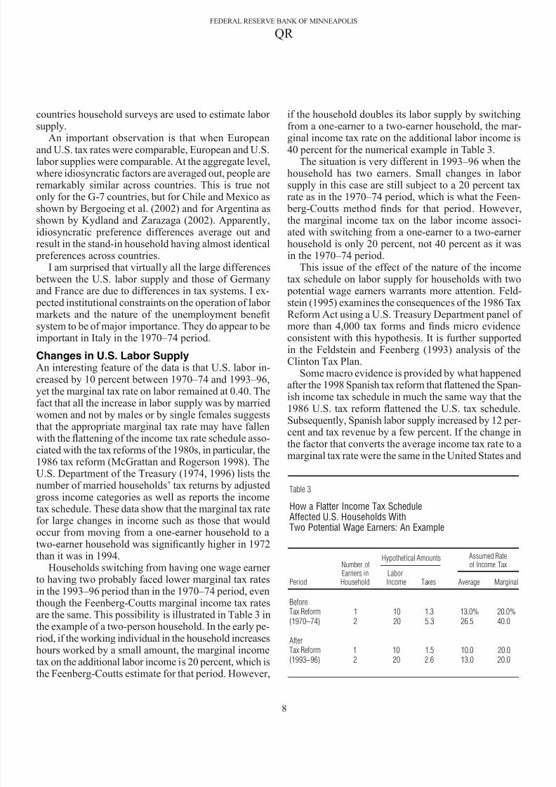
The model economy’s time period is a year. Thesteady state of a pay-as-you-go system and a fullyfunded system are reported in Table 4. With the fullyfunded system, steady-state labor supply is 11 percenthigher, consumption 17 percent higher, and welfare inlifetime consumption equivalents 9 percent higher. The

problem with just switching from the current pay-as-you-go system to a fully funded system is that the initialold would suffer. The following reform makes all betteroff. There are still better reforms than this one, in par-ticular, plans that have tax rates that depend upon ageat the time of reform.

Proposed ReformPeople are given the option to continue with the currentsystem or to shift to a new system. With the new system,8.7 percent of wage income is put into an individualaccount with the government that earns a 4 percent realreturn. Upon retirement, savings in this account areannuitized. Effectively, people have the option to havetheir tax rate on labor reduced from 40 percent to 31.3

percent and to save 8.7 percent of their labor income ina government retirement account or to continue withthe current social security system. With the reform, non–

social security transfers are left unchanged.Steady-state social security liabilities of the pay-

as-you-go system are large: 4.62 times gross nationalincome (GNI). With the reform, those aged 37 andyounger choose the new system. The welfare gain to the22-year-old at the time of the change exceeds 4 percentin lifetime consumption equivalents. Associated with

the change, the annual capital/output ratio increasesfrom 2.7 to 3.3, as seen in Table 5. This increase takes45 years.

Table 5 also shows that pension liabilities of the pay-as-you-go system are large: 2.30 times GNI. With thenew system, the decline steadily becomes zero 35 yearsafter the reform.

Some Equity ConsiderationsIn the model, all individuals earn the same wage when,in fact, some people earn higher wages than others.Given that earning a 4 percent after-tax real return is anattractive investment, equity considerations suggest anupper bound on contributions. Similarly, lower-incomehouseholds should have the right to contribute more than8.7 percent of their labor income.

Still another consideration is how to deal with mar-ried couples. An equitable solution is that each party hasan account and household contributions are split equally

between the two accounts with the contribution limitdiscussed above applying to an individual account andnot to a household account. Some will be so unfortunatethat the amount in their account will be insufficient to

provide for a minimal acceptable retirement. This sug-

Table 4

Effects of a Shift to a Fully FundedSocial Security System

Steady States in a Model With Each System

Soc. Sec. EffectiveCapital

Labor ConsumptionLiabilities

Labor TaxSystem Output Output Supply Per Person Net Output Welfare* Rate

Pay-As-You-Go 100 2.77 100 100 4.62 100 40.0%

Fully Funded 123 4.91 111 117 0 109 27.05

*Welfare here is measured in lifetime consumption equivalents.




Edward C. Prescott

11

gests adding means-tested supplementary benefits.Why force people to save, as this scheme does? The

answer is that it gets around the time inconsistency problem. Some individuals will not save if they knowthat others will provide for their consumption whether

the others are taxpayers, family members, or charities.Concluding RemarksIn the process of determining the effect of differencesin effective marginal labor tax rates on labor supplyacross countries and time in the advanced industrialcountries, I have estimated the elasticity of labor supplyand have found it to be large, nearly 3 when the fractionof time allocated to the market is in the neighborhoodof the current U.S. level. This estimate of the elasticityis essentially the same one needed to account for busi-ness cycle fluctuations. That this elasticity is large is

good news. If labor supply were inelastic, the advancedindustrial countries would face a cruel choice of eitherincreasing taxes on the young, thereby lowering young

people’s welfare, or not honoring the promises made tothe old, making the old worse off.

The large labor supply elasticity means that as popu-lations age, promises of payments to the current andfuture old cannot be financed by increasing tax rates.These promises can be honored by reducing the effectivemarginal tax rate on labor and moving toward retire-ment systems with the property that benefits on marginincrease proportionally to contributions. Requiring

people to save for their retirement years is not a tax anddoes not reduce labor supply. My example establishes

that reforms are possible that benefit the current youngworkers and future workers while honoring promisesmade to the old.

One factor that I ignored in my social security reformexample is that a larger capital/labor ratio increases wag-es with any reasonable aggregate production function.If this factor is taken into consideration, the welfaregains are larger. It is beyond the scope of this article tomore than scratch the surface of how best to reform thesocial security retirement system and what the resultingwelfare gains would be. But it is clear, given the highresponsiveness of labor supply to marginal labor tax

rates, that the potential gains are great.

Table 5

Effects of a Shift to an Optimal GovernmentIndividual Retirement Account

For 60 Years After Reform, Assuming WorkersAged 15–37 Years Choose the New Account

Soc. Sec.Liabilities Capital

Year Output Output

1 2.30 2.71

15 1.57 2.80

30 .63 3.08

45 0 3.31

60 0 3.32




QR

12

AppendixData Sources

1. Source of national accounts (SNA) statistics: United Na-tions (1982, 2000).

2. Source of civilian employment, noncivilian employment,annual hours per employee, population aged 15–64: OECDLabour Database, available at http://www.oecd.org/home/.Follow links to Statistics, Labour, and Labour Force Sta-tistics—Data.

“Hours of work: manufacturing” data are used for Japanin 1970–71 because annual hours per employee for Japanin 1970–71 are not in the OECD Labour Database. Thesedata are obtained from United Nations (1981). They are based on establishment study.

3. Source of purchasing power parity GDP numbers in Table1: OECD Annual National Accounts Statistics, Table B.3(OECD 2001), available at http://www.sourceoced.org.Follow links to Statistics, OECD Statistics, and NationalAccounts.

4. Source of income taxes and contributions for Social Se-curity, United States: BEA Table 3.2., available at

http://www.bea.gov/bea/dn/nipaweb/SelectTable.asp?Selected=Y#S3.

5. Source of national accounts statistics for Spain: Instituto Nacional de Estadística (Spain Statistical Office), availableat http://www.ine.es/inebase/menu3i.htm#15.

Download the annual national accounts for the period1993–2001.




Edward C. Prescott

13

References

Auerbach, Alan J., and Kotlikoff, Laurence J. 1987. Dynamic fiscal policy. Cam- bridge: Cambridge University Press.

Baxter, Marianne, and King, Robert G. 1993. Fiscal policy in general equilibrium. American Economic Review 83 (June): 315–34.

Bergoeing, Raphael; Kehoe, Patrick J.; Kehoe, Timothy J.; and Soto, Raimundo. 2002. A decade lost and found: Mexico and Chile in the 1980s. Review of

Economic Dynamics 5 (January): 166–205.

Boldrin, Michele; Christiano, Lawrence J.; and Fisher, Jonas D. M. 2001. Habit persistence, asset returns, and the business cycle. American Economic Review 91 (March): 149–66.

Chari, V. V.; Kehoe, Patrick J.; and McGrattan, Ellen R. 2003. Accounting for the

Great Depression. Federal Reserve Bank of Minneapolis Quarterly Review 27 (Spring): 2–8.

Christiano, Lawrence J., and Eichenbaum, Martin. 1992. Current real-business-cycle theories and aggregate labor-market fluctuations. American Economic

Review 82 (June): 430–50.

Cole, Harold L., and Ohanian, Lee E. 1999. The Great Depression in the UnitedStates from a neoclassical perspective. Federal Reserve Bank of MinneapolisQuarterly Review 23 (Winter): 2–24.

___________. 2002. The Great U.K. Depression: A puzzle and possible resolution. Review of Economic Dynamics 5 (January): 19–44.

Conesa, Juan Carlos, and Garriga, Carlos. 2003. Status quo problem in Social Secu-rity reforms. Macroeconomic Dynamics 7 ( November): 691–710.

Cooley, Thomas F., ed. 1995. Frontiers of business cycle research. Princeton:Princeton University Press.

Davis, Steven J., and Henrekson, Magnus. 2003. Tax effects on work activity, indus-try mix and shadow economy size: Evidence from rich-country comparisons.Manuscript. University of Chicago Graduate School of Business.

Feenberg, Daniel R., and Coutts, Elisabeth. 1993. An introduction to the TAXSIMmodel. Journal of Policy Analysis and Management 12 (Winter): 189–94.

Feldstein, Martin. 1995. The effect of marginal tax rates on taxable income: A panel study of the 1986 Tax Reform Act. Journal of Political Economy 103(June): 551–72.

Feldstein, Martin, and Feenberg, Daniel R. 1993. Higher tax rates with little revenuegain: An empirical analysis of the Clinton tax plan. Tax Notes 58 (March):1653–57.

Fisher, Jonas D. M., and Hornstein, Andreas. 2002. The role of real wages, produc-tivity, and fiscal policy in Germany’s Great Depression 1928–1937. Reviewof Economic Dynamics 5 (January): 100–27.

Hansen, Gary D. 1985. Indivisible labor and the business cycle. Journal of Monetary Economics 16 (November): 309–27.

Kehoe, Timothy J., and Prescott, Edward C. 2002. Great depressions of the 20th

century. Review of Economic Dynamics 5 (January): 1–18.Kydland, Finn E., and Prescott, Edward C. 1982. Time to build and aggregate fluc-

tuations. Econometrica 50 (November): 1345–70.

Kydland, Finn E., and Zarazaga, Carlos E. J. M. 2002. Argentina’s lost decade. Review of Economic Dynamics 5 (January): 152–65.

Lucas, Robert E., Jr. 1972. Expectations and the neutrality of money. Journal of Economic Theory 4 (April): 103–24.

Lucas, Robert E., Jr., and Rapping, Leonard A. 1969. Real wages, employment, andinflation. Journal of Political Economy 77 (September/October): 721–54.

Maddison, Angus. 1995. Monitoring the world economy: 1820–1992. Develop-ment Centre Studies. Paris: Organisation for Economic Co-operation andDevelopment.

McGrattan, Ellen R., and Prescott, Edward C. 2000. Is the stock market overvalued? Federal Reserve Bank of Minneapolis Quarterly Review 24 (Fall): 20–40.

___________. 2002. Taxes, regulations, and the value of U.S. corporations: A generalequilibrium analysis. Research Department Staff Report 309. Federal Reserve

Bank of Minneapolis, August. ___________. 2003. Average debt and equity returns: Puzzling? American Economic

Review 93 (May): 392–97.

McGrattan, Ellen R., and Rogerson, Richard. 1998. Changes in the hours workedsince 1950. Federal Reserve Bank of Minneapolis Quarterly Review 22(Winter): 2–19.

Mendoza, Enrique G.; Razin, Assaf; and Tesar, Linda L. 1994. Effective tax rates inmacroeconomics: Cross-country estimates of tax rates on factor incomes andconsumption. Journal of Monetary Economics 34 (December): 297–323.

Mendoza, Enrique G., and Tesar, Linda L. 2002. Tax competition v. tax coordinationunder perfect capital mobility: The supply-side economics of international taxcompetition. CEPR 4th Conference of the Analysis of International Capital

Markets Research Training Network , November.

Nickell, Stephen. 2003. Employment and taxes. Manuscript. Venice InternationalInstitute.

Organisation for Economic Co-operation and Development (OECD). 2001. Nationalaccounts of OECD countries, volume I: Main aggregates, CD-ROM onbeyond 20/20. Paris: Organisation for Economic Co-operation and Develop-ment, January.

Olovsson, Conny. 2003. Why do Europeons work so little? Manuscript. InternationalInstitute for Economic Studies, Stockholm University.

Rogerson, Richard D. 2003. The employment effects of taxes. Working paper pre-sented at Dynamic Economics Conference in Honor of Edward C. Prescott,29 April, Federal Reserve Bank of Chicago.

United Nations. 1981. 1979/80 statistical yearbook, 31st issue. Department of Inter-national Economic and Social Affairs. New York: United Nations.

___________. 1982. Yearbook of national accounts statistics 1980, Part 1 and Part2. New York: United Nations.

___________. 2000. National accounts statistics: Main aggregates and detailedtables. New York: United Nations.

U.S. Department of the Treasury, Internal Revenue Service. 1974. Statistics of

income, individual income tax returns 1972. Washington, D.C.: U.S. Govern-ment Printing Office.

___________. 1996. Statistics of income, individual income tax returns 1994.Washington, D.C.: U.S. Government Printing Office.

Documents

Why Americans work more than Europeans