Embed Size (px)
Citation preview

¦ 2014 � vol. 10 � no. 1
TTTThe QQQQuantitative MMMMethods for PPPPsychology
T
Q
M
P
13
When to Use Hierarchical Linear Modeling Veronika Huta ����, a
a School of psychology, University of Ottawa
AbstractAbstractAbstractAbstract � Previous publications on hierarchical linear modeling (HLM) have provided guidance on how to perform the analysis, yet there is relatively little information on two questions that arise even before analysis: Does HLM apply to one’s data and research question? And if it does apply, how does one choose between HLM and other methods sometimes used in these circumstances, including multiple regression, repeated-measures or mixed ANOVA, and structural equation modeling or path analysis? The purpose of this tutorial is to briefly introduce HLM and then to review some of the considerations that are helpful in answering these questions, including the nature of the data, the model to be tested, and the information desired on the output. Some examples of how the same analysis could be performed in HLM, repeated-measures or mixed ANOVA, and structural equation modeling or path analysis are also provided.
Keywords Keywords Keywords Keywords � hierarchical linear modeling; multilevel modeling; repeated-measures; analysis of variance; structural equation modeling; path analysis
���� [email protected]
IntroductionIntroductionIntroductionIntroduction
Hierarchical linear modeling (HLM) (also referred to as
multilevel modeling, mixed modeling, and random
coefficient modeling) is a statistical analysis that many
researchers are becoming interested in. Previous
publications on HLM have provided detailed
information on how to perform the analysis (e.g.,
Raudenbush, Bryk, Cheong, Congdon, & du Toit, 2011;
Woltman, Feldstain, MacKay, & Rocchi, 2012). Yet there
is relatively little information to help researchers
decide whether HLM applies to their data and research
question, and how to choose between HLM and
alternative methods of analyzing the data. The purpose
of this tutorial is to review some of the considerations
that are helpful in answering these questions. I will
focus specifically on the analyses that can be carried out
by the software called HLM7 (Raudenbush, Bryk, &
Congdon, 2011).
HLM applies to randomly selected grHLM applies to randomly selected grHLM applies to randomly selected grHLM applies to randomly selected groupsoupsoupsoups
HLM applies when the observations in a study form
groups in some way and the groups are randomly
selected (Raudenbush & Bryk, 2002).
There are various ways of having grouped data. For
example, there may be multiple time points per person
and multiple persons – these data are grouped because
multiple time points are nested within each person.
There may be multiple people per organization and
multiple organizations, such that people are nested
within organizations. There can even be multiple
organizations per higher-order group, such as schools
nested within cities.
It is possible to have a grouping hierarchy with 2, 3,
or 4 levels. An example of a four-level hierarchy is
multiple students per school, multiple schools per city,
multiple cities per county, and multiple counties – here
students are the Level 1 units, schools are the Level 2
units, cities are the Level 3 units, and counties are the
Level 4 units. In this tutorial, for the sake of simplicity, I
will focus primarily on two-level hierarchies.
As noted above, HLM applies to the situation when
the groups are selected at random, i.e., when they
represent a random factor rather than a fixed factor.
For example, if a study has ten schools (with multiple
students in each school), then schools are a random
factor if they are randomly selected and the aim is to
generalize to the population of all schools; in contrast,
schools are a fixed factor if the researcher specifically
wanted to draw conclusions about those ten schools,
and not about schools in general (and the analysis then
becomes an ANOVA).
HLM is an HLM is an HLM is an HLM is an expanded form of regressionexpanded form of regressionexpanded form of regressionexpanded form of regression
HLM is essentially an expanded form of regression. In
most HLM analyses, there is a single dependent
variable, though a multivariate option exists as well
within the HLM7 software; the dependent variable can
be quantitative and normally distributed, or it can be
qualitative or non-normally distributed. In this tutorial,
I will focus on the case of a single dependent variable
that is normally distributed.
Suppose the data set consists of 100 participants,
studied at 50 time points each. Roughly speaking, HLM

¦ 2014 � vol. 10 � no. 1
TTTThe QQQQuantitative MMMMethods for PPPPsychology
T
Q
M
P
14
obtains what is called a Level 1 (or within-group)
regression equation for each participant, based on that
individual’s 50 time points (for a total of 100
equations); the Level 1 equation may have one or more
Level 1 independent variables (i.e., independent
variables measured at each time point), or it may have
no independent variables (the same set of independent
variables must be used in all Level 1 equations); the
dependent variable must be measured at each time
point. Like any regression, the Level 1 equation for a
given individual summarizes their data across 50 time
points into just a few coefficients: an intercept (which
equals the participants’ mean score on the dependent
variable if the researcher uses what is called group
mean centering for each Level 1 independent variable, a
common procedure), and a slope for each of the Level 1
independent variables. Each of these coefficients – the
intercept and possibly some slopes – then serves as the
dependent variable in a Level 2 (or between-group)
regression equation; for example, if there are two
independent variables in the Level 1 equations, there
will be three regression equations at Level 2, one
predicting the Level 1 intercept, one predicting the
Level 1 slope for one Level 1 independent variable, and
the other predicting the slope for the other Level 1
independent variable. Each Level 2 equation has an
intercept (which equals the mean intercept or slope
across all participants if the researcher uses what is
called grand mean centering for each Level 2
independent variable, a common procedure), and it
may have one or more Level 2 independent variables
(i.e., independent variables measured just once for each
participant).
For example, suppose again that there are 100
participants, with 50 time points each, the dependent
variable is state well-being (s_wbeing – HLM truncates
variable names to eight characters, so you might as well
create short names to begin with), the Level 1
independent variable is state autonomy (s_auton), and
the Level 2 independent variable is trait extraversion
(t_extrav). Below is what the regression equation looks
like at Level 1. (Note that e is the error term, indicating
that the observed state well-being score at a given time
point may differ from the well-being score predicted for
that person based on the regression equation; e is
always present in the Level 1 equation.)
The intercept (π0) and the slope (π1) values will
differ from participant to participant. If state autonomy
is group mean centered, the π0 conveniently equals the
mean well-being score across all time points for a given
participant, and thus provides an estimate of the
participant’s trait level of well-being.
Below is what the regression equations look likes at
Level 2. (Note that in HLM, you can choose whether or
not to include the error term r0 and/or r1; if the error
term r0 is included, this implies that the intercept π0 is
assumed to differ from person to person; if the error
term r1 is included, this implies that the slope π1 is
assumed to differ from person to person.)
Figure 1 shows a screen shot of how the model would
appear in HLM.
Each equation at Level 2 is a summary across all 100
participants, and each of the four coefficients (those
indicated with the letter β) is tested to determine if it
differs significantly from zero. If trait extraversion is
grand mean centered, β00 conveniently equals the mean
well-being score across all time points and across all
participants, called the grand mean, and thus provides
an estimate of the average participant’s trait level of
well-being. The β10 value provides the average π1 value
across all participants (assuming the Level 2
independent variable(s) is/are grand mean centered).
If β10 is statistically significant, then on average across
Figure 1 � Sample two-level Hierarchical Linear Model.

¦ 2014 � vol. 10 � no. 1
TTTThe QQQQuantitative MMMMethods for PPPPsychology
T
Q
M
P
15
participants, state autonomy significantly relates to
state well-being. The β01 value gives the relationship
between trait extraversion and trait well-being
(assuming group mean centering was used). Finally, if
β11 is significantly different from zero, this indicates
that trait extraversion moderates the strength of the
relationship between state autonomy and state well-
being (this moderation is also called a cross-level
interaction, since trait extraversion at Level 2 is
interacting with state autonomy at Level 1; it is
certainly possible to have an interaction between
independent variables at the same level, but these are
product terms that must be created in the data set
before importation into HLM).
When HLM When HLM When HLM When HLM is superior to regular regressionis superior to regular regressionis superior to regular regressionis superior to regular regression
In the past, before HLM was developed, people
simply used a single regular regression for grouped
data – either what is called a Level 1 regression or what
is called a Level 2 regression. Suppose there are 100
participants and 50 time points per participant, with
the variables at each level as discussed before. A Level 1
regression can be used when the researcher is only
interested in relationships at Level 1 (e.g.., does state
autonomy relate to state well-being), and it involves
simply running a regression with a sample size of all
5000 data points as if they came from 5000
independent participants. A Level 2 regression can be
used when the researcher is only interested in
relationships at Level 2 (e.g., does trait extraversion
relate to trait well-being), and it involves running a
regression on 100 data points, one per participant, after
computing the mean well-being score for each
participant.
The question is: When are these regular regressions
problematic, making HLM a preferable choice?
When HLM is superior to Level 1 regression – the
problem of inflated Type I error
A Level 1 regression treats data from 100 participants
as if it were data from 5000 independent participants.
Therein lies the problem. This can lead to a large
inflation of Type I error, since the statistical significance
of a result depends on sample size. HLM deals with this
problem by basing its sample size for inferential
statistics on the number of groups (100 in this
example), not on the total number of observations
(5000 in this example).
The HLM approach has a drawback of its own, as the
reader might guess. HLM tends to be on the
conservative side when testing relationships at Level 1,
i.e., it has less power than a Level 1 regression would.
There usually is some degree of dependence among
the observations from a given group, however, and it is
usually advisable to apply an analysis for grouped data,
such as HLM. Only if there is no dependence is it
appropriate to conduct a Level 1 regression. It is
possible to determine the degree of within-group
dependence in HLM by testing whether there is
variance in the Level 1 intercept across groups – if it
does not vary, an analysis for grouped data is not
necessary and one can use a Level 1 regression, though
one may still want to proceed with an analysis for
grouped data on theoretical grounds or for consistency
with other analyses that are being conducted.
Alternatively, an Intraclass Correlation Coefficient (ICC)
smaller than 5% suggests that an analysis for grouped
data is unnecessary (Bliese, 2000). The ICC is the
proportion of the total variance in the dependent
variable (which is the sum of the between-group
variance and the within-group variance) that exists
between groups.
When HLM is superior to Level 1 regression – the
value of differentiating Levels 1 and 2
In addition to the reduction of Type I error, there is also
a conceptual reason to use HLM instead of Level 1
regression whenever there is a significant variance in
coefficients across groups. HLM allows the researcher
to separate within-group effects from between-group
effects, whereas a Level-1 regression blends them
together into a single coefficient.
For example, in one study, I ran an experience-
sampling study with about 100 participants and about
50 time points per participant (Huta & Ryan, 2010). At
Level 1, I measured eudaimonia (the pursuit of
excellence) and hedonia (the pursuit of pleasure).
When I analyzed the data properly, using HLM, I
obtained the following results. At Level 1, so at a given
moment in time, a person’s degree of state eudaimonia
and state hedonia correlated negatively, around -.3.
Thus, if a person is momentarily striving for excellence,
they are probably not simultaneously striving for
pleasure. However, at Level 2, so at the trait level, a
person’s average degree of eudaimonia over the 50
time points and their average degree of hedonia over
the 50 time points actually correlated positively, about
.30! Thus, if a person often strives for excellence, they
also tend to often strive for pleasure. (The latter
analysis was performed by choosing one variable, say
¦ 2014 � vol. 10 � no. 1
TTTThe QQQQuantitative MMMMethods for PPPPsychology
T
Q
M
P
16
hedonia, as the dependent variable for HLM, and then at
Level 2 using each person’s mean eudaimonia score as
the independent variable, with the mean eudaimonia
scores being computed for each participant before
running the HLM – in other words, HLM can compute
the mean score on the dependent variable for each
person, but the mean score on the independent variable
has to be computed person by person prior to running
HLM). If the data had simply been analyzed using a
Level-1 regression, the correlation between eudaimonia
and hedonia would be -.10, which is part way between -
.3 and +.3 and tells us little about the true correlation at
Level 1 or at Level 2.
Figure 2 provides an illustration of how the correct
slopes obtained through HLM at Levels 1 and 2 can be
in opposite directions from each other, and how the
Level 1 regression slope is a blend of the two slopes
obtained through HLM. Each dotted ellipse represents
data across multiple time points for each participants
(only three participants are shown). The thin dotted
lines running through the dotted ellipses are the lines
of best fit for each participant. The thick dotted line is
the mean of all the thin dotted lines across participants,
and corresponds to the Level 1 or “within-person”
correlation of -.3 I obtained using HLM. The thin solid
ellipse encompasses all of the data combined across
participants, and the thin solid line is the line of best fit
through this data and corresponds to the somewhat
uninformative correlation of -.1 obtained through a
Level 1 regression. The thick solid line corresponds to
the Level 2 or “between person” correlation of +.3
obtained using HLM (or using a Level 2 regression), and
is the line of best fit through the center points (called
centroids) of the ellipses for each participant, which are
indicated by large dots.
When HLM is When HLM is When HLM is When HLM is superior to Lsuperior to Lsuperior to Lsuperior to Level 2 evel 2 evel 2 evel 2 regressionregressionregressionregression
Let me continue with the example of 100
participants and 50 time points per participant, and
both eudaimonia and hedonia being measured at each
time point. Recall that a Level-2 regression involves
taking the mean dependent variable score and the
mean independent variable score across the 50 time
points for each participant, which produces just 100
observations in total, and then running a regular
regression on those means. The results of a Level 2
regression and of HLM will be the same if each
participant has the same number of time points and no
missing data (and the same variance in the dependent
variable). But one lovely feature of HLM is that it allows
the researcher to have different numbers of
observations per group (i.e., per participant in this
example) and furthermore gives greater weight to the
groups with more observations (and less variance),
which produces slightly more accurate estimates of
population values. The greater the differences in
sample size (and variance) across groups, the greater
the advantage of HLM relative to Level-2 regression.
This benefit is subtler and less crucial than the
advantage of HLM over Level 1 regression, but it is
hedonia Correct HLM
Level 2 slope
i.e., slope between
people
Correct HLM
Level 1 slopes
i.e., slopes within people
Incorrect Level 1
Regression slope
mixing between- &
within-person slopes
eudaimonia
Figure 2 ���� How two variables can have a negative relationship at the within-group level but a positive relationship
at the between-group level in Hierarchical Linear Modeling.

¦ 2014 � vol. 10 � no. 1
TTTThe QQQQuantitative MMMMethods for PPPPsychology
T
Q
M
P
17
worth being aware of.
When it is appropriate to use HLM on data from
dyads
When comparing HLM with regular regression, I
would like to also make a comment about dyads. Dyads
always have two members per group, e.g., husband and
wife, caregiver and patient, coach and athlete. It is a
common assumption that all research on dyads should
be analyzed using HLM. This is often true but not
always. HLM only applies when exactly the same set of
variables – the dependent variable, or the dependent
variable and some Level 1 independent variables – is
measured in all members of the group, i.e., in both
members of the dyad. For example, HLM applies when
the same marital satisfaction questionnaire is given to
both the husband and the wife. However, if different
variables have been assessed in the two members of the
dyad – for example, if the dependent variable assessed
in the caregiver is burnout, but the dependent variable
assessed in the patient is depression – then HLM does
not apply and one would simply run a regular
regression (or some other analysis) to predict caregiver
burnout, and a separate analysis to predict patient
depression.
Different Different Different Different analyses for grouped dataanalyses for grouped dataanalyses for grouped dataanalyses for grouped data
HLM is not the only method available for dealing with
grouped data. The two most common alternatives are
structural equation modeling (SEM) (or its simpler
version, path analysis), and a general linear model
(GLM) with a repeated-measures variable, which I will
simply refer to as repeated-measures. Examples of the
latter include: mixed design ANOVA/GLM with a
repeated-measures/within-subjects variable that is
analogous to the dependent variable measured
repeatedly at Level 1 in HLM, and one or more
between-subjects variables that are analogous to the
Level 2 independent variables in HLM; repeated-
measures ANOVA/GLM with a repeated-
measures/within-subjects variable; and a paired-
samples t-test, which has only two repeated measures.
A less well-known alternative is functional data analysis
(FDA), and there are others still, such as growth
mixture modeling (GMM).
Let me outline FDA and GMM only briefly, just
enough to make the reader aware of these options. I
will then discuss repeated measures and SEM (and path
analysis) in more detail, describing how the same
research question would be addressed with these
methods as well as HLM, and listing criteria that can
help a researcher choose between HLM, repeated
measures, and SEM.
Functional data analysis
Developed by Ramsay and Silverman (2002, 2005),
FDA is used specifically for longitudinal data. It is more
flexible than other approaches in that it models the
precise pattern of fluctuations that a variable
undergoes over time, and every individual/entity can
have a different pattern. This makes FDA more flexible
than the other approaches I am comparing it with,
which assume that a single function (e.g., a straight line,
a quadratic curve, a cubic curve, exponential decay) can
represent the entire span of data points, and that all
individuals can be represented by the same function.
For example, Figure 3 shows the pattern of depression
scores over the course of therapy for four individuals. A
smoothing process can then be applied, to a degree
gauged by the researcher, in hopes of eliminating minor
fluctuations that are likely to represent random noise,
and retaining major fluctuations that are likely to
represent a true signal.
Figure 3 � How Functional Data Analysis models the fluctuations a variable undergoes over time.

¦ 2014 � vol. 10 � no. 1
TTTThe QQQQuantitative MMMMethods for PPPPsychology
T
Q
M
P
18
The entire pattern for each individual can then be
used in various analyses. For example, analogous to an
independent-samples t-test, it is possible to test
whether two groups of individuals (such as those in
cognitive therapy versus those in behavioral therapy)
differ significantly in terms of their mean score at a
given therapy session, or even in terms of their slope or
rate of improvement (referred to as the velocity of the
curve at that time point). Analogous to a regression, it is
possible to test whether fluctuations in one variable
over time (such as social support) predict later
fluctuations in another variable (such as well-being). A
principal components analysis can also be performed
on the patterns to see at what time points
individuals/entities differ most widely from each other
– for example, when studying depression scores over
the course of therapy, the greatest spread in scores
occurs during the last few therapy sessions, since some
clients continue to get better while others have trouble
with therapy termination and their symptoms get
worse.
Growth Mixture Modeling
Unlike HLM, repeated-measures, SEM, and FDA,
which are variable-centered approaches, GMM is a
person-centered approach (Jung & Wickrama, 2008).
Variable-centered approaches focus on relationships
among variables (another example is factor analysis).
Person-centered approaches, such as GMM and cluster
analysis, focus on similarities between individuals and
aim to classify participants into groups based on their
responses across a set of variables. GMM is used for
longitudinal data, and it analyzes the trajectories of
different individuals to determine whether there are
subgroups within which individuals have similar
trajectories (Wang & Bodner, 2007). For example,
when analyzing depression scores over the course of
therapy, GMM might indicate that there are two groups
of individuals – those whose scores progressively
improve, and those whose scores remain about the
same. Latent class growth analysis is a special case of
GMM which assumes that all individuals within a given
group have exactly the same trajectory, rather than
allowing for variability within groups the way GMM
does (Jung & Wickrama, 2008).
How to set up the same model in HLM, Repeated-
measures, and SEM – Model A
Suppose a two-level data set with three time points per
participant has state well-being as the dependent
variable at Level 1, and trait extraversion as the
independent variable at Level 2 (suppose there are no
Level 1 independent variables). Suppose the researcher
wishes to test whether there is a significant link
between extraversion and well-being.
Setting up the model in HLMSetting up the model in HLMSetting up the model in HLMSetting up the model in HLM. Prior to importing the data
into HLM (i.e., prior to creating the “mdm,” the
multivariate data matrix), there would be one data set
for the Level 1 data (with one line per time point) and a
separate data set for the Level 2 data (with one line per
participant), as shown in Figure 4 if one is using SPSS
(IBM Corp., 2011a).
Figure 4 � How to set up the Level 1 and Level 2 data sets for Model A in SPSS prior to using the HLM software for
Hierarchical Linear Modeling.
¦ 2014 � vol. 10 � no. 1
TTTThe QQQQuantitative MMMMethods for PPPPsychology
T
Q
M
P
19
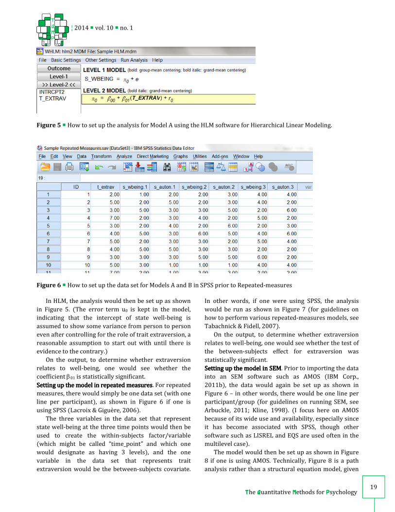
In HLM, the analysis would then be set up as shown
in Figure 5. (The error term u0 is kept in the model,
indicating that the intercept of state well-being is
assumed to show some variance from person to person
even after controlling for the role of trait extraversion, a
reasonable assumption to start out with until there is
evidence to the contrary.)
On the output, to determine whether extraversion
relates to well-being, one would see whether the
coefficient β01 is statistically significant.
Setting up the model in repeated measuresSetting up the model in repeated measuresSetting up the model in repeated measuresSetting up the model in repeated measures. For repeated
measures, there would simply be one data set (with one
line per participant), as shown in Figure 6 if one is
using SPSS (Lacroix & Giguère, 2006).
The three variables in the data set that represent
state well-being at the three time points would then be
used to create the within-subjects factor/variable
(which might be called “time_point” and which one
would designate as having 3 levels), and the one
variable in the data set that represents trait
extraversion would be the between-subjects covariate.
In other words, if one were using SPSS, the analysis
would be run as shown in Figure 7 (for guidelines on
how to perform various repeated-measures models, see
Tabachnick & Fidell, 2007).
On the output, to determine whether extraversion
relates to well-being, one would see whether the test of
the between-subjects effect for extraversion was
statistically significant.
Setting up the model in SEMSetting up the model in SEMSetting up the model in SEMSetting up the model in SEM. Prior to importing the data
into an SEM software such as AMOS (IBM Corp.,
2011b), the data would again be set up as shown in
Figure 6 – in other words, there would be one line per
participant/group (for guidelines on running SEM, see
Arbuckle, 2011; Kline, 1998). (I focus here on AMOS
because of its wide use and availability, especially since
it has become associated with SPSS, though other
software such as LISREL and EQS are used often in the
multilevel case).
The model would then be set up as shown in Figure
8 if one is using AMOS. Technically, Figure 8 is a path
analysis rather than a structural equation model, given
Figure 5 � How to set up the analysis for Model A using the HLM software for Hierarchical Linear Modeling.
Figure 6 � How to set up the data set for Models A and B in SPSS prior to Repeated-measures

¦ 2014 � vol. 10 � no. 1
TTTThe QQQQuantitative MMMMethods for PPPPsychology
T
Q
M
P
20
that it examines the relationships between measured
variables (indicated with rectangles), and not between
latent variables which are factors extracted from
multiple measured variables (which would be indicated
with ellipses). Notice that all three regression
coefficients are constrained to be equal, since they have
all been assigned the same name “a,” so that the
analysis parallels HLM where a single value is obtained
for the link between extraversion and well-being;
similarly, all of the error terms have received the same
label “e1.” Alternatively, the researcher may allow the
regression coefficients and error terms to vary, to see if
the Level 2 independent variable has a different impact
on well-being at each time point, a feature not available
in HLM or repeated-measures.
On the output, to determine whether extraversion
relates to well-being, one would see whether the
regression coefficient “a” was statistically significant.
How to set up the same model in HLM, Repeated-
measures, and SEM – Model B
Now suppose a two-level data set with three time
points per participant has state well-being as the
dependent variable at Level 1, and suppose the
researcher wishes to test whether there is a linear
increasing trend in well-being over time.
Setting up theSetting up theSetting up theSetting up the model in HLMmodel in HLMmodel in HLMmodel in HLM. Prior to importing the data
into HLM, one would need to set up a variable called
“time” in the Level 1 data set, and assign it the values 1,
2, and 3 for time points 1, 2, and 3 (assuming they were
equally spaced), as shown in Figure 9. The Level 2 data
set is also shown in Figure 9 (and is the same as in
Figure 4).
In HLM, the analysis would then be set up as shown
in Figure 10, if one assumes the intercept and slope will
vary from person to person (a good assumption to
begin with, until there is evidence to the contrary).
On the output, to determine whether there is a
linear increasing trend over time, one would see
whether the coefficient β10 is positive and statistically
significant. In other words, one would see whether
there is a relationship between time and state well-
being, on average across participants.
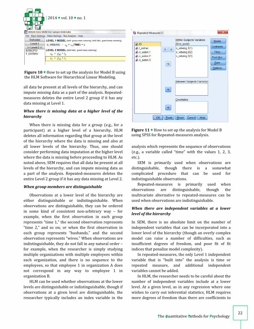
Setting up the model in repeated measuresSetting up the model in repeated measuresSetting up the model in repeated measuresSetting up the model in repeated measures. For repeated
measures, the data set in Figure 6 would be used as is.
The three variables that represent state well-being
would then be used to create the within-subjects
variable, as shown in Figure 11.
On the output, to determine whether there is a
linear trend over time, one would see whether the
within-subjects contrast for time_point is statistically
significant. One would also need to check the
descriptive statistics or a plot, to see if the linear trend
was indeed increasing rather than decreasing.
Setting up the model in SEMSetting up the model in SEMSetting up the model in SEMSetting up the model in SEM. For SEM, the data structure
shown in Figure 6 would be used as is.
When using the AMOS software to run the SEM, the
model would be set up as shown in Figure 12 (which is
Figure 7 � How to set up the analysis for Model A using
SPSS for Repeated-measures analysis.
Figure 8 � How to set up the analysis for Model A using
AMOS for Path Analysis.

¦ 2014 � vol. 10 � no. 1
TTTThe QQQQuantitative MMMMethods for PPPPsychology
T
Q
M
P
21
called a latent difference score analysis – e.g., Hawley,
Ho, Zuroff, & Blatt, 2007; McArdle, 2001). The terms in
ellipses would be created by the researcher, and the
two paths from “Sn” would be constrained to be equal,
by being assigned the same coefficient “a.” (The “d”
values are the latent and error-free variables assumed
to produce the measured variables; the “delta d” values
are the differences in the “d” values from one time point
to the next, being equal to the later time point minus
the earlier time point, thus the term latent difference
score analysis; “Sn” is the latent slope assumed to
underlie the “delta d” values; and the regression
coefficients “a” are fixed to be equal – typically all set to
1 – to reflect the expectation that change over time will
be linear for each participant.)
On the output, to determine whether there is an
increasing linear trend over time, one would see
whether the coefficient “a” is positive and statistically
significant.
Choosing Choosing Choosing Choosing betweenbetweenbetweenbetween HLM, RepeatedHLM, RepeatedHLM, RepeatedHLM, Repeated----measures, and SEMmeasures, and SEMmeasures, and SEMmeasures, and SEM
Let me now review a variety of criteria that come into
play when choosing a method for analyzing grouped
data. The focus will be on HLM, repeated-measures, and
SEM, as these are the most commonly used methods.
Sometimes more than one method is possible, but I will
emphasize the situations where one method is
preferable to another.
In reading the criteria below, it will become clear
that I was quite selective in creating Models A and B
above to compare across HLM, repeated measures, and
SEM. Only certain models and data sets can be analyzed
using all three methods. It will also become clear that
choosing an acceptable method is a complex process,
with many considerations to take into account. Some
considerations are rigid and can entirely rule out a
method, whereas other considerations are more
flexible and the ultimate selection of method will rely
on the judgment of the researcher.
When the hierarchy has three or more levels
Hierarchies with three or more levels are typically
analyzed using HLM, though if sample sizes are small at
all the lower levels of a hierarchy, it may also be
feasible to use SEM. Repeated-measures only applies to
two-level hierarchies.
When sample size differs from group to group
Of the three analyses, only HLM can be used when
sample size differs from group to group at any of the
lower levels of a hierarchy.
When there is missing data at Level 1
Missing data at Level 1 can be handled by HLM, which
can simply work with the data it is given, if the
researcher chooses the “delete when running analyses”
option when importing data into HLM. (There is also an
option to delete an entire Level 2 group if it has any
missing data at Level 1, if the researcher chooses the
“delete when making mdm” option). SEM requires that
Figure 9 � How to set up the Level 1 and Level 2 data sets for Model B in SPSS prior to using the HLM Software for
Hierarchical Linear Modeling.
¦ 2014 � vol. 10 � no. 1
TTTThe QQQQuantitative MMMMethods for PPPPsychology
T
Q
M
P
22
Figure 10 � How to set up the analysis for Model B using
the HLM Software for Hierarchical Linear Modeling.
Figure 11 � How to set up the analysis for Model B
using SPSS for Repeated-measures analysis.
all data be present at all levels of the hierarchy, and can
impute missing data as a part of the analysis. Repeated-
measures deletes the entire Level 2 group if it has any
data missing at Level 1.
When there is missing data at a higher level of the
hierarchy
When there is missing data for a group (e.g., for a
participant) at a higher level of a hierarchy, HLM
deletes all information regarding that group at the level
of the hierarchy where the data is missing and also at
all lower levels of the hierarchy. Thus, one should
consider performing data imputation at the higher level
where the data is missing before proceeding to HLM. As
noted above, SEM requires that all data be present at all
levels of the hierarchy, and can impute missing data as
a part of the analysis. Repeated-measures deletes the
entire Level 2 group if it has any data missing at Level 2.
When group members are distinguishable
Observations at a lower level of the hierarchy are
either distinguishable or indistinguishable. When
observations are distinguishable, they can be ordered
in some kind of consistent non-arbitrary way – for
example, when the first observation in each group
represents “time 1,” the second observation represents
“time 2,” and so on; or when the first observation in
each group represents “husbands,” and the second
observation represents “wives.” When observations are
indistinguishable, they do not fall in any natural order –
for example, when the researcher is simply studying
multiple organizations with multiple employees within
each organization, and there is no sequence to the
employees, so that employee 1 in organization A does
not correspond in any way to employee 1 in
organization B.
HLM can be used whether observations at the lower
levels are distinguishable or indistinguishable, though if
observations at a given level are distinguishable, the
researcher typically includes an index variable in the
analysis which represents the sequence of observations
(e.g., a variable called “time” with the values 1, 2, 3,
etc.).
SEM is primarily used when observations are
distinguishable, though there is a somewhat
complicated procedure that can be used for
indistinguishable observations.
Repeated-measures is primarily used when
observations are distinguishable, though the
multivariate alternative to repeated-measures can be
used when observations are indistinguishable.
When there are independent variables at a lower
level of the hierarchy
In SEM, there is no absolute limit on the number of
independent variables that can be incorporated into a
lower level of the hierarchy (though an overly complex
model can raise a number of difficulties, such as
insufficient degrees of freedom, and poor fit of fit
indices that penalize model complexity).
In repeated-measures, the only Level 1 independent
variable that is “built into” the analysis is time or
repeated measure, and additional independent
variables cannot be added.
In HLM, the researcher needs to be careful about the
number of independent variables include at a lower
level. At a given level, as in any regression where one
wishes to carry out inferential statistics, HLM requires
more degrees of freedom than there are coefficients to

¦ 2014 � vol. 10 � no. 1
TTTThe QQQQuantitative MMMMethods for PPPPsychology
T
Q
M
P
23
be estimated (in at least some of the groups, though not
necessarily all). Consider the Level 1 equation below:
There are three coefficients in this equation – the
intercept π0 and the two slopes π1 and π2 – and
therefore a minimum of four observations is required.
Another way of summarizing this is as follows: if there
are K independent variables, HLM requires K + 2
observations. Thus, if a given level of the hierarchy
consists of dyads, there are only two observations per
group and there is no room for independent variables
at that level!
When there are too few observations for the
number of independent variables at Level 1, some
researchers artificially increase the number of
observations (e.g., Maguire, 1999) by treating
individual items or subscales of items on the dependent
variable measure as if they were separate
measurements of the dependent variable. For example,
if a researcher has dyads at Level 1 and the dependent
variable is a four-item scale, the researcher could treat
each of the four items as if it were a separate
observation of the dependent variable, which would
artificially boost the sample size at Level 1 to eight
observations per dyad. Alternatively, if a researcher has
dyads at Level 1, the dependent variable is an 18-item
scale, and one wants to boost the sample size to six
observations per dyad, one can create three parallel
subscales of the dependent variable (as highly inter-
correlated as possible), and treat each of them as if it
were a separate measurement of the dependent
variable. Researchers may vary in their comfort level
with this practice of boosting the number of
measurements of the dependent variable, but the
practice is more acceptable to the degree that the items
or subscales of the dependent variable measure the
same concept – if their content is diverse, the practice is
harder to justify. Naturally, the strategy is only possible
if the dependent variable is a multi-item scale.
When there are independent variables at the highest
level of the hierarchy
All three analysis – HLM, repeated-measures, and SEM –
can handle any number of independent variables at the
highest level of the hierarchy (within reason – the
number of independent variables should not take up a
large fraction of the degrees of freedom at that level,
and with too many independent variables, one starts to
run into the problem of over-fitting, i.e., the equation
starts modeling a lot of the noise rather than primarily
the signal in the data).
When one wishes to test cross-level interactions
Suppose a researcher wishes to test a cross-level
interaction, such that trait extraversion moderates the
effect of state autonomy on state well-being. This can
easily be tested in HLM, and the software itself will
create the interaction term, the researcher does not
need to create it in the data beforehand. SEM can also
test a cross-level interaction, but the researcher needs
to create all the interaction terms in the data set before
analysis (unless the higher level independent variable
is a qualitative one, such as gender, in which case the
SEM model can be run once for each gender, and
differing results for the two genders indicate an
interaction), and SEM quickly begins to consume many
degrees of freedom as the number of observations at
the lower level increases. Both HLM and SEM can test
interactions between two independent variables in
non-adjacent levels of a hierarchy, such as Levels 1 and
3, as well as interactions between independent
variables at three or more levels (though SEM is likely
to consume even more degrees of freedom than for
two-way interactions). In Repeated-measures, the only
cross-level interaction possible is one between the
repeated measure variable at Level 1 (e.g., time_point)
and a between-subjects variable at Level 2 (e.g.,
t_extrav).
In repeated-measures, since the only independent
variable possible at Level 1 is time or repeated
measure, the only cross-level interaction possible is an
Figure 12 � How to set up the analysis for Model B using
AMOS for Path Analysis.
¦ 2014 � vol. 10 � no. 1
TTTThe QQQQuantitative MMMMethods for PPPPsychology
T
Q
M
P
24
interaction between time/repeated measures and a
between-person independent variable, which is tested
directly by the software, the researcher does not need
to create an interaction term in the data.
When one wishes to test same-level
interactions
Both HLM and SEM can test interactions at the
same level, but the interaction terms must be
created in the data before analysis. Repeated-
measures can only test interactions at Level 2,
since it cannot have multiple independent
variables at Level 1.
When the model does not have a multiple
regression structure
Both HLM and repeated-measures require a
multiple regression structure, such that one or
more independent variable(s), and possibly
some interactions between them, all directly
predict a single dependent variable (or a
composite of dependent variables). For any
model more complex than a multiple
regression, SEM is most often used. For
example, SEM is appropriate when a variable
in the model predicts more than one other
variable, or when a variable serves both as an
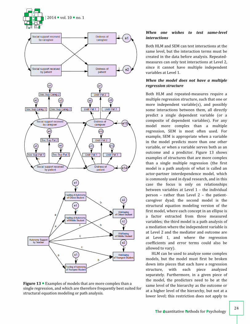
outcome and a predictor. Figure 13 shows
examples of structures that are more complex
than a single multiple regression (the first
model is a path analysis of what is called an
actor-partner interdependence model, which
is commonly used in dyad research, and in this
case the focus is only on relationships
between variables at Level 1 – the individual
person – rather than Level 2 – the patient-
caregiver dyad; the second model is the
structural equation modeling version of the
first model, where each concept in an ellipse is
a factor extracted from three measured
variables; the third model is a path analysis of
a mediation where the independent variable is
at Level 2 and the mediator and outcome are
at Level 1, and where the regression
coefficients and error terms could also be
allowed to vary).
HLM can be used to analyze some complex
models, but the model must first be broken
down into pieces that each have a regression
structure, with each piece analyzed
separately. Furthermore, in a given piece of
the model, the predictors need to be at the
same level of the hierarchy as the outcome or
at a higher level of the hierarchy, but not at a
lower level; this restriction does not apply to
Figure 13 � Examples of models that are more complex than a
single regression, and which are therefore frequently best suited for
structural equation modeling or path analysis.

¦ 2014 � vol. 10 � no. 1
TTTThe QQQQuantitative MMMMethods for PPPPsychology
T
Q
M
P
25
SEM.
The set of complex models that repeated-measures
could apply to is extremely restricted. It would again
require that the model be broken into pieces with a
regression structure. Furthermore, the last regression
in a causal chain could only have Level 2 variables
predicting a Level 1 outcome (unless there is one
predictor and it is time point or repeated measure), and
all preceding steps in the causal chain would be
analyzed using regular regressions with Level 2
variables predicting a Level 2 outcome.
When the sample size is too small (or too large)
Restrictions in sample size at one or more levels of the
hierarchy may also push the researcher away from
certain analysis options. Ideally, one would use a power
analysis software to determine the sample size
required at each level to achieve adequate power. (One
software applicable to HLM is Optimal Design, which is
available for free on the internet, at
http://sitemaker.umich.edu/group-based/optimal_
design_software; one software that is applicable to
repeated-measures is G*Power, also available for free
on the internet, at http://www.psycho.uni-
duesseldorf.de/abteilungen/aap/gpower3/download-
and-register; power analysis for SEM is less well
established.) Nevertheless, there are some general
guidelines that can help a person determine whether a
sample size may be adequate for HLM, repeated-
measures, and/or SEM.
Sample size required at each level in HLM. Sample size required at each level in HLM. Sample size required at each level in HLM. Sample size required at each level in HLM. At a lower
level of the hierarchy, HLM can work with as few as two
observations per group if there are no independent
variables at that level, or as few as K+2 observations if
there are K independent variables, as noted earlier.
Many papers have been published with just two, three,
or four observations per group, so these sample sizes
are quite common. To reach 80% power, however,
group sizes often need to be 15 or greater (though 5 or
10 is sometimes sufficient). To be able to reliably report
the regression equations of individual groups (which is
done only occasionally, e.g., when there are multiple
students per school and each school would like to know
the results for that particular school), the required
sample size is often closer to 50.
At the highest level of the hierarchy, having an
adequate sample size is more critical, since it is the
sample size at this level which influences the power of
the analyses. In other words, the number of groups at
the highest level needs to be large enough for the
results to be generalizable to the population of all
groups. Some publications have had Level 2 sample
sizes as small as 10 or 20, and in some research areas
(e.g., work with animals or brain scans) this is difficult
to avoid. To reach 80% power, however, sample sizes
upward of 60 are typically required.
Sample size required at each level in repeatedSample size required at each level in repeatedSample size required at each level in repeatedSample size required at each level in repeated----measures. measures. measures. measures.
At Level 1, repeated-measures can work with any
sample size of 2 or greater.
At Level 2, to reach 80% power, sample sizes above
60 are often required.
Sample size required at each level in SEM. Sample size required at each level in SEM. Sample size required at each level in SEM. Sample size required at each level in SEM. At a lower
level of the hierarchy, SEM can have as few as 2
observations per group, and does not require that there
be K+2 observations for K independent variables, as
noted earlier. If there are too many observations, the
SEM model will use too many degrees of freedom
unless corresponding regression coefficients are
constrained to be equal and corresponding error terms
are constrained to be equal (as shown in the third
model of Figure 14).
At the highest level of the hierarchy, SEM typically
requires a larger sample size than does HLM or
repeated-measures. Recommendations vary widely, but
most people would agree that 100 is a bare minimum,
and the more common recommendation is 200 or
more; alternatively, many people use Bentler and
Chou’s (1987) suggestion that there be at least 5
observations per free parameter.
When the researcher seeks certain information in
the output
Thus far I have discussed considerations that relate
to the nature of the data or the nature of the model to
be tested, when choosing between HLM, repeated-
measures, and SEM. These analyses also differ in the
information that appears on the output, so I will now
review some of these differences. I will not provide an
exhaustive list of the differences, I will only focus on
one major difference that is commonly of interest: HLM
provides information based on how coefficients differ
across groups (i.e., how coefficients at one level of the
hierarchy differ across units of a higher level of the
hierarchy), whereas repeated-measures and SEM
provide information about how coefficients differ
across repeated measures.
A separate regression equation foA separate regression equation foA separate regression equation foA separate regression equation for each groupr each groupr each groupr each group. Only
HLM provides a separate regression equation for each
higher-level group – for example, if there are multiple
organizations and multiple employees within each

¦ 2014 � vol. 10 � no. 1
TTTThe QQQQuantitative MMMMethods for PPPPsychology
T
Q
M
P
26
organization, HLM can provide the regression equation
across employees within a given organization. (This is
an additional option that must be requested when
running the analysis, and the coefficients of the
equations can be obtained from an SPSS file generated
with the name “resfil.”) HLM actually provides several
versions of these regression equations – the Ordinary
Least Squares (OLS) version simply provides the
coefficients that would be obtained if a regular
regression were run on the data within a given group;
an Empirical Bayes version provides coefficients for a
given group that are influenced by the average
coefficients when summarizing across all groups, to the
degree that the data for the given group are unreliable,
i.e., based on a small sample size and/or highly
variable; and a more fine-tuned Conditional Empirical
Bayes version, which provides coefficients for a given
group that are influenced by coefficients in groups that
have similar characteristics to the group in question.
Reliability of a coefficient to determine whether the Reliability of a coefficient to determine whether the Reliability of a coefficient to determine whether the Reliability of a coefficient to determine whether the
regression equation for each group can beregression equation for each group can beregression equation for each group can beregression equation for each group can be reported reported reported reported
reliablyreliablyreliablyreliably. Only HLM provides an estimate of the average
reliability, across groups, of each lower level coefficient.
Among other things, this reliability informs the
researcher whether the regression equations of
individual groups can be reported (the reliability
ranges from 0 to 1, and values in the neighborhood of
.80 suggest that individual regressions can be
reported).
Variance of a coefficient across groupsVariance of a coefficient across groupsVariance of a coefficient across groupsVariance of a coefficient across groups. Only HLM
reports the variance of each coefficient across groups,
and tests the significance of this variance (e.g., for a
three-level hierarchy, the output indicates how much
Level 1 coefficients vary across Level 2 units, how much
Level 1 coefficients vary across Level 3 units, how
much Level 2 coefficients vary across Level 3 units, and
how much cross-level interactions between Level 1 and
2 independent variables vary across Level 3 units).
Among other things, a significant variance in a
coefficient across units of a higher level provides
statistical justification for adding independent variables
at the higher level in hopes of accounting for some of
that variance.
Correlations between coefficients across groupsCorrelations between coefficients across groupsCorrelations between coefficients across groupsCorrelations between coefficients across groups. Only
HLM provides the correlations between lower level
coefficients across groups. For example, if a research
has a two-level hierarchy where the dependent variable
is depression severity and the Level 1 independent
variable is time, a negative correlation between the
Level 1 intercept and slope indicates that the more
severe the depression, the faster/steeper the decrease
in depression over time.
A separate regression coefficient for each repeated A separate regression coefficient for each repeated A separate regression coefficient for each repeated A separate regression coefficient for each repeated
measuremeasuremeasuremeasure. If a researcher wishes to know whether the
slope of the relationship between a predictor and
outcome differs across repeated measurements of that
predictor and outcome, the researcher would require
SEM. For example, in the third diagram of Figure 14, a
researcher may wish to determine whether the link
between a feeling of autonomy and well-being differs
for the oldest, youngest, and middle student – in that
case, the researcher would simply remove the letter “b”
from each regression arrow and thereby allow the
coefficient to vary.
SEM can also be used to determine whether a
higher-level independent variable relates differently to
the dependent variable for each repeated measure. For
example, in Figure 14, this would be accomplished by
removing the constraint “a” on the link between teacher
autonomy support and each student’s feeling of
autonomy, thereby allowing the strength of the link to
vary. Repeated-measures can similarly show how the
link between a Level 2 independent variable and the
dependent variable differs across repeated measures, if
one requests the parameter estimates option.
Variance of the dependent variable across repeated Variance of the dependent variable across repeated Variance of the dependent variable across repeated Variance of the dependent variable across repeated
measuresmeasuresmeasuresmeasures. If a researcher wishes to know whether the
mean score on the dependent variable varies across
repeated measurements, they would use repeated-
measures (and leave out any Level 2 independent
variables). The between-subjects effect for the
intercept would indicate whether this variance is
significant.
SummarySummarySummarySummary
In sum, Hierarchical linear modeling (HLM) applies to
data that are grouped in some way, such as: multiple
cities, with multiple schools within each city, and
multiple students within each school. In this example,
cities would be referred to as Level 3 of the hierarchy,
schools would be referred to as Level 2, and students
would be referred to as Level 1. In addition, HLM
applies when the groups (e.g., cities and schools) are
randomly selected, such that the researcher’s aim is to
generalize to the results to the population of all groups.
The HLM method is an expanded form of regression,
whereby a separate regression is obtained within each
group, and the dependent variable is always measured
at the lowest level of the hierarchy. The coefficients
(intercept and slopes) from the within-group

¦ 2014 � vol. 10 � no. 1
TTTThe QQQQuantitative MMMMethods for PPPPsychology
T
Q
M
P
27
regressions then serve as dependent variables in
several regressions at the between-group level. In this
way, all of the main effects and interactions a
researcher might be interested in can be determined:
the main effect of a within-group independent variable,
the main effect of a between-group independent
variable, the interaction between independent
variables at the same level of the hierarchy, and the
interaction between independent variables at different
levels of the hierarchy.
Analysis using HLM (or another method used for
grouped data) preserves the multi-level nature of the
data, and thus has several advantages over a single
regression performed on the data. The greatest
advantage is that a grouped analysis protects the
researcher against inflated Type I error.
In addition to HLM, methods that sometimes apply
to grouped data include repeated-measures analyses
(such as mixed design ANOVA/GLM) and structural
equation modeling (SEM) or its simpler version path
analysis (and possibly even functional data analysis,
Growth mixture modeling or Latent Class Growth
Analysis, or other options). This paper provided two
examples of models that could be set up in HLM,
repeated-measures, and SEM/path analysis, and
outlines how the data set and analysis for each method
would be set up.
This paper then provides considerations that can
help a researcher in choosing between HLM, repeated-
measures, and SEM/path analysis if they have grouped
data. These considerations include: the number of
levels in the hierarchy, sample size, missing data,
distinguishability of group members, the number of
independent variables, the nature of the interactions to
be tested, whether the model to be tested has a
regression structure, and the information one desires
on the output (e.g., whether one is more interested in
differences between groups or differences between
repeated measures).
Together, the information in this paper sheds some
light on a frequently neglected topic: how a researcher
can decide whether HLM applies to their data and
research question, and how a researcher can choose
between HLM and alternative methods of analyzing
such data.
ReferencesReferencesReferencesReferences
Arbuckle J. L. (2011). AMOS 20.0 user’s guide.
Crawfordville, FL: Amos Development Corporation.
Bentler, P. M., & Chou, C. P. (1987) Practical issues in
structural modeling. Sociological Methods &
Research, 16, 78-117.
Bliese, P. D. (2000). Within-group agreement, non-
independence, and reliability: implications for data
aggregation and analysis. In K. J. Klein, & S. W. J.
Kozlowski (Eds.), Multi-level theory, research and
methods in organizations: Foundations, extensions,
and new directions (pp. 349–381). San Francisco,
CA: Jossey-Bass.
Hawley, L. L., Ho, M. R., Zuroff, D. C., & Blatt, S. J. (2007).
Stress reactivity following brief treatment for
depression: Differential effects of psychotherapy
and medication. Journal of Consulting and Clinical
Psychology, 75, 244–256.
Huta, V., & Ryan, R. M. (2010). Pursuing pleasure or
virtue: The differential and overlapping well-being
benefits of hedonic and eudaimonic motives. Journal
of Happiness Studies, 11, 735-762.
IBM Corp. (2011a). IBM SPSS Statistics for Windows,
Version 20.0. Armonk, NY: IBM Corp.
IBM Corp. (2011b). IBM SPSS AMOS, Version 20.0.
Armonk, NY: IBM Corp.
Jung, T., & Wickrama, K. A. S. (2008). An introduction to
Latent Class Growth Analysis and Growth mixture
modeling. Social and Personality Psychology
Compass, 2, 302–317.
Kline, R. B. (1998). Principles and practice of structural
equation modeling. New York, NY: Guilford.
Lacroix, G. L., & Giguère, G. (2006). Formatting data files
for repeated-measures analyses in SPSS: Using the
Aggregate and Restructure procedures. Tutorials in
Quantitative Methods for Psychology, 2, 20-25.
Maguire, M.C. (1999). Treating the dyad as the unit of
analysis: A primer on three analysis approaches.
Journal of Marriage and the Family, 61, 213-223.
McArdle, J. J. (2001). A latent difference score approach
to longitudinal dynamic analysis. In R.
Cudeck, S. Du Toit, & D. Sörbum (Eds.), Structural
equation modeling: Present and future (pp. 341–
380). Lincolnwood, IL: Scientific Software
International.
Ramsay, J. O., & Silverman, B. W. (2002). Applied
functional data analysis: Methods and case studies.
New York: Springer.
Ramsay, J. O., & Silverman, B. W. (2005). Functional
data analysis, Second Edition. New York:
Springer.
Raudenbush, S. W., & Bryk, A. S. (2002). Hierarchical
Linear Models: Applications and data analysis
methods, Second Edition. Newbury Park, CA: Sage.
¦ 2014 � vol. 10 � no. 1
TTTThe QQQQuantitative MMMMethods for PPPPsychology
T
Q
M
P
28
Raudenbush, S. W., Bryk, A. S., Cheong, Y. F., Congdon, R.
T., & du Toit, M. (2011). HLM7: Hierarchical
Linear and Nonlinear Modeling. Chicago, IL:
Scientific Software International.
Raudenbush, S. W., Bryk, A. S., & Congdon, R. (2011).
HLM7 for Windows [Computer software]. Skokie, IL:
Scientific Software International, Inc.
Tabachnick, G. G., and Fidell, L. S. (2007). Experimental
designs using ANOVA. Belmont, CA: Duxbury.
Wang, M., & Bodner, T. E. (2007). Growth mixture
modeling: Identifying and predicting unobserved
subpopulations with longitudinal data.
Organizational Research Methods, 10, 635-656.
Woltman, H., Feldstain, A., MacKay, J. C., & Rocchi, M.
(2012). An introduction to hierarchical linear
modeling. Tutorials in Quantitative Methods for
Psychology, 8, 52-69.
CitationCitationCitationCitation
Huta, V. (2014). When to Use Hierarchical Linear Modelling. The Quantitative Methods for Psychology, 10 (1), 13-28.
Copyright © 2014 Huta. This is an open-access article distributed under the terms of the Creative Commons Attribution License (CC BY). The use, distribution or
reproduction in other forums is permitted, provided the original author(s) or licensor are credited and that the original publication in this journal is cited, in
accordance with accepted academic practice. No use, distribution or reproduction is permitted which does not comply with these terms.
Received: 6/04/12 ~ Accepted: 27/06/13