“WHEN I USE A WORD…” PRO-POOR GROWTH AND POVERTY REDUCTION.

Louise Cord, J. Humberto Lopez, and John Page The World Bank

August 2003

This paper critically reviews the debate on pro poor growth. Using new data that focuses on long run spells of growth and poverty reduction we demonstrate that poverty outcomes differ widely relative to the overall rate of growth across regions and countries. We also find that in a number of countries long run growth spells have been associated with increases in poverty. From this evidence we conclude that economic growth alone does not guarantee sustained poverty reduction.. For “pro-poor growth” to take place policies must be both pro-growth and pro-poor.

JEL Classification: I32; O15. Key Words: Poverty, Growth, Pro-poor growth, Income Distribution

Please Address Correspondence to: Louise J. Cord, Poverty Reduction Group, The World Bank. 1818 H. Street, NW, Washington, DC, USA, 20433. Phone: 202-473-0969. Fax: 202-522-7496 Email: Lcord@worldbank.org

“WHEN I USE A WORD…” PRO-POOR GROWTH AND POVERTY REDUCTION.

Louise Cord, J. Humberto Lopez, and John Page

The World Bank1 Development practitioners and policy makers are fond of the term “pro-poor growth” because, rather like Humpty Dumpty in Alice’s Wonderland, to each of them “it means exactly what [they] want it to mean.” In preparing this paper we found references to pro-poor growth by organizations as diverse as the GTZ and the Vatican, each defining the concept differently, but each advocating it as an important (or primary) objective of public policy in low-income countries. Can a concept that “means so many different things” provide a useful guide for public policy? And, if so, how should it be defined and used? One common thread running through all of the competing definitions of pro-poor growth is an assumption that historically the poor have failed to benefit proportionately – or in its most extreme form at all – from the growth experiences of low income countries. Simple theory and empirical evidence indicate that poverty reduction can be achieved by accelerating economic growth and/or by changing the distribution of income. We know that sustained economic growth reduces poverty. This is not to say, however, that average growth translates one for one into growth of the incomes of the poor in every single growth episode in every country.2 The origins of the current interest in pro-poor growth, thus, lie in the attempt to understand the empirical significance and factors behind the variable impact of growth on poverty reduction.

In this paper we demonstrate that rates of poverty reduction relative to the

overall rate of economic growth differ widely across regions and countries. Moreover, we find that in a number of countries long run growth spells, defined as sustained growth for more than ten years have been associated with increases in poverty. From this evidence we conclude that economic growth and growth-oriented policies, while necessary for sustained poverty reduction, do not guarantee that it will occur at the country level. For “pro-poor growth” to take place policies must be both pro-growth and pro-poor.

The remainder of the paper is organized in five sections. In Section I we survey the definitional debate on “pro-poor growth.” Section II examines the argument that accelerating the rate of growth in low income countries is sufficient to achieve sustained poverty reduction. Section III uses new econometric evidence to establish the empirical relevance of distributional change to poverty reduction and to show that the per capita income of the bottom quintile of the income distribution is a robust predictor

1 The findings and opinions expressed in this paper are those of the authors. They do not represent the views of the World Bank, its member countries or its Executive Directors. 2 Ravallion (2001) for example finds that, based on cross country evidence, the 95% confidence interval for a 1% increase in average household income or consumption yields anything from a modest drop in the poverty rate of 0.6% to a more dramatic 3.5% decline

of headcount poverty. Section IV uses this result to explore the diversity of regional and country experiences with the long-run relationship between growth and poverty reduction. Section V concludes. I. Defining Pro-Poor Growth.

Pro-poor growth has been broadly defined by a number of international organizations as growth that leads to significant reductions in poverty (OECD, 2001 and UN, 2000). But what is a significant reduction in poverty? How much must the poor benefit for growth to be considered pro-poor? In attempting to give analytical and operational content to the concept two broad definitions have of pro- poor growth have emerged.

The first draws on the literal meaning of the phrase: growth is pro-poor when the poor benefit disproportionately from it. In some formulations this criterion is met if the rate of income growth of the poor exceeds the rate of income growth of the non-poor. A stricter definition would hold that the absolute income gains of the poor must exceed those received by the non-poor. In both cases, however, in order for growth to be pro-poor, it must be accompanied by a decrease in inequality.3 McCulloch and Baulch (2000), Kakwani and Pernia (2000) and Kakwani and Son (2001) all offer a measures of pro-poor growth that focus on reducing inequality.

The second definition discards the literal interpretation of the concept for a more general, but very much less strict formulation: growth is pro-poor if it reduces poverty. Kraay (2003) for example advocates that growth is pro-poor if the poverty measure of interest declines. Ravallion and Chen (2003) measure pro-poor growth as the mean growth rate of income of the poor. Using this second definition growth will always be pro-poor except when the incomes of the poor are stagnant or decline leading to an increase in the poverty measure.

For public policy purposes neither definition of pro-poor growth is fully satisfactory. The two formulations imply widely divergent interpretations of what constitute successful economic outcomes. Definitions based on more rapid relative or absolute income growth for the poor run the risk of ignoring overall economic performance and the fortunes of the non-poor. This is inconsistent with efforts to maximize the welfare of society at large and can lead to undesirable public choices. For example, a society attempting to achieve pro-poor growth under the first definition would favor an outcome characterized by a rate of per capita income growth of 2 percent if the average income of the poor grew at 3 percent, over an outcome where the average rate of growth was 6 percent and the average income of the poor grew at 4 percent.

Definitions based on the second set of criteria on the other hand run the risk of

under weighting the welfare of the poor. If pro-poor growth can be asserted to have occurred, no mater how small the actual gains to the poor, progress toward such internationally agreed objectives as the Millennium Development Goals may be painfully slow. Positive but low growth of income among the poor would appear to be 3 Klassen (2003) provides a survey of definitions and an evaluation of their relative merits.

inconsistent with a strong commitment to poverty reduction. Even under this second, less restrictive definition it is relevant to inquire how the rate of reduction in poverty or the rate of income growth of the poor stacks up, both relative to historical trends and to the current rate of growth of average income.

Seeking a single measure of pro-poor growth that addresses these concerns,

Klasen (2003) revives a measure first developed by Ahluwhalia and Chenery (1974) – the distributionally weighted growth rate. This is a weighted average of growth rates across different income groups (defined by deciles or quintiles) in which greater weights are assigned to the income growth of the poorest quintiles/deciles. The Ahluwhalia-Chenery-Klasen approach succeeds in incorporating broader welfare concerns into a single measure of pro-poor growth, and as an empirical tool to measure how growth benefits a society interested in the welfare of the poor it has substantial promise. It also has a number of drawbacks however: first, the specific weights assigned to income growth among different groups will be difficult to establish; second, since these weights are likely to vary across countries and over time within countries, inter-temporal and inter-country comparisons are difficult; and third, as with any compound index, the results are more difficult to interpret than more disaggregated presentations of the same data.4 In the end we are forced to the conclusion that further debates over the meaning and measurement of “pro-poor growth” are probably counter-productive to the poverty reduction objectives of both low-income countries and the groups advocating that they pursue public policies aimed at achieving them. In the remainder of this paper we will take as a working definition the weaker formulation of pro-poor growth: growth that benefits the poor. As an operational concept this implies that pro-poor growth policies are those that seek to increase the rate of growth of incomes of the poor, either directly by increasing the demand for assets with which the poor are endowed or indirectly by channeling an increasing share of the benefits of economy wide growth toward the poor.

II. Is Growth Enough? In the preceding section we concluded that the most operationally relevant definition of pro-poor growth was simply growth that benefits the poor. There is an important strand of the literature on growth and poverty reduction, however, that argues that on average over time all growth benefits the poor. If this is so, the distinction between growth as a public policy objective and pro-poor growth is a nonsense. Policies designed to maximize the rate of growth in low income countries are likely also to be those that maximize the impact of growth on the poor. The support for this line of argument rests on three simple empirical propositions.. First, Dollar and Kraay (2002) – among several others -- find that that the poor do typically share in rising aggregate income and suffer from economic contractions in the same proportion as everybody else in society. On average growth is

4 For example, Ravallion and Datt’s (2000) “growth incidence curve” conveys much of the same information as the Chenery-Alluwhalia-Klassen approach, but has the advantage of showing the rate of income gains across the whole population.

good for the poor, or at least as good for the poor as for everybody else. Second, growth has been elusive.5 While the international development community may debate whether one growth pattern is more appropriate for the poor than another, the fact is that most poor countries are not growing. Third, in general growth has no apparent systematic impact on income distribution.6 While initial income distributions may be more or less equal, since they do not change as growth takes place, a pro-growth strategy is likely to also be pro-poor. We do not dispute that growth is both good for the poor and necessary for sustained poverty reduction. But is it enough? While it is difficult to argue that sustained poverty reduction can be achieved through redistribution policies alongside economic stagnation, growth associated with progressive distributional changes will have a greater impact in reducing poverty than growth which leaves the distribution unchanged (Bourgignon, 2001). There are two main reasons for this. The first is simply the direct positive impact that progressive distributional change has on poverty reduction for any given rate of growth. There is, however, a second, indirect and positive impact of a fall inequality. Even in the absence of distributional change a given growth rate will have a larger poverty reducing impact if initial inequality is low. Hence, reductions in inequality increase the elasticity of poverty reduction with respect to future growth, and progressive distributional change has both a contemporaneous impact on poverty and a lagged impact by increasing the rate of poverty reduction implied by future growth. Further, it is perfectly possible that regressive distributional change can offset the contemporaneous benefits of growth to the poor and reduce the poverty impact of future growth.

More formally, P=P(y,L(p)), (1) where P is a poverty measure (which for simplicity can be assumed to belong to the Foster-Greer-Thorbecke (FGT) (1984) class), y is per capita income and L(p) is the Lorenz curve measuring the relative income distribution. L(p) is the percentage of income enjoyed by the bottom 100×p percent of the population. 7 Changes in poverty can be decomposed into: dP=∂P/∂y dy+∂P/∂L(p)dL(p). (2)

5 See Easterly (1999) 6 Foster and Szekely (2000), Deininger and Squire (1996), and Ravallion and Chen (1997).

7 The FGT class of poverty measures is given by dxxfz

xzPz

o

)(α

α ∫

−= where α is the parameter

of inequality aversion, z is the poverty line, and x is income. For α= 0, the previous expression reduces to the familiar headcount ratio. When α=1 it weights each poor by his/her distance form the poverty line (the poverty gap), and when α= 2 the weight given to each poor is proportional to the square of the income shortfall (square poverty gap). Put in other words, higher values of α would give more weight to the extreme poor than to those groups closer to the poverty line z.

After some straightforward manipulations (2) can be rewritten as: dP/P=γ dy/y+φdL(p)/L(p), (3) where γ is the growth elasticity of poverty, which measures the percentage change in poverty that takes place when average income increases by one percentage point, and φ is the inequality elasticity of poverty, which measures the percentage change in poverty as a result of a one percent change in the share of income of the lowest pth percentile.

In principle both γ and φ can be expected to be negative.8 That is, both growth and progressive distributional change will lead to poverty reduction with the relative importance of each factor given by the respective elasticities. For example, if γ >φ , a one percent change in income will have a larger impact on poverty reduction than a one percent reduction in inequality. In contrast, if γ <φ a one percent reduction in inequality will have a larger impact on poverty than a one percent change in income. Bringing together elasticities and magnitude of changes one can also express the condition by which poverty will increase as: γ dy/y<φdL(p)/L(p). (4) Observe that (4) does not restrict growth to be negative. In principle it is possible for poverty to increase even when growth is positive. The lower the growth rate the more likely that poverty will increase when inequality increases.

The pro-growth school argues that in practice inequality cannot be expected to change as much as income. However, as noted above the recent growth performance of developing economies has been disappointing. Average per capita growth in low income countries during 1990-2001 was 0.03 percent. This would imply that the expression in the left hand side of (4) is very close to zero, and therefore that small changes in inequality may lead to poverty increases. Thus, the need to pay attention to inequality goes hand in hand with the need to pay attention to growth when one focuses on poverty reduction, especially in low growth economies.

So far we have concentrated on the direct impact that changes in inequality have on poverty reduction, but as noted above there is a second potential impact of changes in inequality. Under the assumption that changes in inequality shift the entire Lorenz curve by a constant proportion of the difference between the actual share in total income accruing to each income group and equal shares, Son and Kakwani (2003) show that ∂ γ/∂y<0, ∂γ/∂G>0, ∂φ/∂y>0, and ∂φ/∂G<0 where G is the Gini index.9 Put in words, both the impact of a given growth rate on poverty reduction and the impact of

8 Strictly speaking for φ to be negative it is also required that the poverty line is below average income. Otherwise progressive distributional change is likely to lead to an increase in poverty. (In the limit, when income is equally distributed all the population would be below the poverty line and therefore be poor.) 9 ∆L(p)=τ(p-L(p)). (5) In (5) τ would the proportional change in the Gini index. This assumption basically rules out the possibility of improvements in inequality due to redistribution from the extremely rich to the very (but not extremely) rich.

progressive distributional change on poverty reduction increase with the level of development and decrease with the level of inequality of the country in question

Table 1 presents computed elasticities of headcount poverty to growth under the assumption that the income distribution can be approximated by a log-normal density function10. The elasticities are computed for different Gini coefficients (running from .3 to .6) and different levels of development (expressed in terms of the poverty line as a percentage of per capita GDP). Table 1 suggests that in a country where the poverty line is about 33 percent of per capita income and the Gini coefficient is .3, the growth elasticity would be –3.9 (i.e. growth of one percent of GDP would reduce poverty by almost 4 percent). In contrast, if the same country had high inequality, say a Gini of .6, the growth elasticity of poverty would be -.8. Thus, high initial inequality levels are likely to represent a barrier to poverty reduction since the impact of growth on poverty will be much smaller than in countries with a more equal income distribution. A similar result can also be obtained for the inequality elasticity of growth.

Whether these concerns are more than mere analytical qualifications to a robust empirical, pro-growth story, however, depends on the degree to which we find empirically that inequality matters in the relationship between long run growth and poverty reduction. That is the subject of our next section. III. Inequality, Growth, and Poverty Reduction

In order to shed light on the empirical relationship between growth, inequality and poverty we rely on two databases.11 The first database we use is that of Dollar and Kraay (2002). This database contains 418 observations for 133 countries of the income shares by quintile of the population. The second database contains 366 observations on headcount poverty (US$1 (PPP) per day poverty line) for 42 countries. This database includes, in addition to the poverty measures, average survey income. However, it does not report inequality data. We have merged the information in both databases and have also computed the share of income that would accrue to the lowest quintile of the population for each of the 366 observations in the poverty database.

With these data in hand we have estimated five models relating changes in poverty to growth and changes in inequality. The econometric results are reported in Table 2. Column (1) reports the results of a naïve model that links the percentage change in poverty to growth only. Columns (2) to (5) aim at capturing the impact of both growth and distributional change on poverty.

In column (2) we regress changes in poverty on growth in the income levels of

the lowest quintile of the population, which in turn depends on the evolution of average income and of the share of average income of the lowest quintile. Econometrically this model imposes the restriction that changes in inequality (as given by changes in the share of income of the lowest quintile of the population) and changes in average income have the same impact on poverty. It is also worth noting that the specification

10 If the distribution of income y is log-normal, then log(y)~N(µ,σ), with G= 2 Φ(σ/√2)-1 where Φ(.) denotes the cumulative normal distribution (Aitchinson and Brown (1966)). 11 We would like to thank Aart Kray for providing us with both databases.

in column (2) relates an absolute definition of poverty, where the poor are those with income levels below a US$1 (PPP) threshold, to a relative concept of poverty, the income level of a pre-specified proportion of the population (in this case the lowest quintile). 12 To the best of our knowledge this is the first time that this relationship has been explored.13

In column (3) we replicate a model first estimated by Ravallion (1997) where growth rates are interacted with one minus the Gini coefficient. This model, in effect, incorporates the possibility of heterogeneous growth elasticities of poverty in a cross section regression framework in line with the discussion above (i.e. the impact of growth on poverty reduction is a decreasing function of inequality as measured by the Gini). This model does not allow for changes in inequality. To some extent, however, the comparison of the econometric results in columns (2) and (3) will give us information regarding the relative importance of the direct and indirect impact of inequality on growth.

In columns (4) and (5) we report the results of two econometric models that include changes in inequality in addition to growth. In these equations we do not restrict the impact of inequality to have any particular value (other than being constant across time periods). Two alternative measures of inequality are considered. Column (4) considers changes in the (log) Gini. Column (5) considers changes in the (log) of the income share of the lowest quintile of the population. Notice also that (5) is an unrestricted version of (2).

In the majority of empirical work on growth-poverty outcomes individual observations are defined as spells – the interval between two household surveys. Because surveys are undertaken at irregular intervals across countries this approach results in both an unbalanced panel of data in which some countries have multiple observations while others have only a single spell and a relatively short term focus,

12 Strictly speaking many of the studies using absolute definitions of poverty are based on per capita expenditure levels and use income levels only as a substitute on data availability grounds. 13 The poverty literature has focused on two approaches to analyze the poverty growth links. The first approach uses a relative concept of poverty by which the poor are assumed to be a pre-specified proportion of the population –usually the lowest quintile of the population- and analyzes how the income levels of this group evolve in time . Examples of this approach include Dollar and Kraay (2002) and Timmer (1997). The second approach uses an absolute definition of poverty where the poor are defined as those with income levels below a pre-specified threshold; this threshold may be common for all countries under analysis (for example PPP adjusted US$1 per person per day) or be country specific (for example when the threshold is based on the purchase cost of subsistence package which by definition is country specific). Examples of this approach are Ravallion (2000) and Bruno et al. (1998). It must be acknowledged that both absolute and relative concepts of poverty have some limitations: (i) once a cut off is defined all the individuals in a given group (poor or rich) are treated equally regardless of where they are located within their group (i.e. those among the poorest one percent are treated –at least statistically– as those with income levels only marginally below the poverty threshold; similarly those among the richest one percent have the same weight as those with income only marginally above the threshold level); (ii) relative definitions of poverty applied to a cross section of countries will treat in a similar fashion a Spaniard and an Honduran in the lowest quintile of their respective country distributions, no matter that Spain has per capita income levels (US$20,000) that are eight fold those of Honduras (US$2,500); and (iii) absolute definitions of poverty are extremely sensitive to the pre-specified income threshold (i.e. defining a subsistence level is far from obvious and will depend to some extend of what is meant by poor in a given country).

since the interval between household surveys in the majority of countries is often less than five years.

Our interest, however, centers on the long-run relationship between economic

growth and poverty reduction. For this reason Table 2 reports the results of estimating these models for three different sub-samples, reflecting differing approaches to the use of the household survey and income data. The first sub-sample considers all the spells in the database; this is the orthodox approach outlined above. The second sub-sample takes a longer term approach and only considers one spell per country spanning all periods between the first and the last available survey. This transformation reduces the number of observations to 42. Finally, the third sub-sample takes an even longer term approach and considers countries for with there are at least five years between the first and last available survey. This approach reduces the number of cross section observations to 32.

The results in Table 2 provide a strong case for the empirical relevance of

inequality to poverty reduction. All coefficient estimates in Table 2 are of expected sign and are significant at conventional levels. Including a variable that captures changes in inequality significantly improves the explanatory power of the regressions. For example, if one considers the sample including all spells, the model in column (2) (which interacts average income growth with changes in the share of income of the lowest quintile of the population) has an R2 that is 14 percentage points higher than the model including only growth (.51 against .37). The same explanatory power (.51) is obtained with the model in column (4) (which in addition to growth also includes the changes in the (log) Gini without any parameter restriction). The specification reported in the last column (5) -- where in addition to growth we include changes in the (log) share of income of the lowest quintile of the population (also unrestricted) – provides the best fit.

The ranking in terms of goodness of fit is basically maintained for all specifications in the long-spells and extra long-spells samples, although the differences are now less striking. Models (1) and (3) have the lowest adjusted R2 and models (2), (4) and (5), those that in addition to growth consider changes in inequality, perform very similarly. In particular, the differences in overall explanatory power between models (2) and (5) are relatively small.

Comparison of the corrected R2 and coefficient estimates between samples

suggests that the length of growth-poverty spells is in fact relevant for evaluating the poverty reducing impact of growth and distributional change. The percentage of the variance explained by the regressions increases substantially for all specifications as we move from short growth-poverty spells to longer ones. In general the elasticities of poverty reduction with respect to both income growth and distributional change also rise with the length of the spell interval. This is particularly marked in specifications (2) and (4) where the elasticity of poverty reduction with respect to changes in the measure of distribution rises as the length of spell increases. This provides some support for the argument outlined above that progressive distributional change has both a contemporaneous and a lagged effect on the extent to which it benefits the poor

Three summary messages emerge from this analysis. First, while growth is good for the poor, inequality changes also are empirically relevant in explaining changes in poverty. Second, the income of the lowest quintile of the population does an excellent job of tracking changes in absolute poverty. For long run spells, changes in the income of the lowest quintile of the population alone explain more than 70 percent of the variance in poverty. This result is particularly welcome if interest centers on exploring poverty outcomes over long periods of time. Given the limited availability of absolute poverty data, more extensively available income distribution and income data can be used to track absolute poverty trends. Third, the data suggest that both the explanatory power and the coefficient estimates of the regressions are not invariate to the length of spell chosen as an observation in the cross-country data. Higher elasticities and better fit are associated with longer spell intervals. IV. Inequality and Pro-Poor Growth: A Look at the Evidence.

The cross-country-regression-based evidence reviewed above indicates both growth and inequality play a significant role in explaining changes in poverty, particularly in the long run. It does not address, however, the concern that seems to underlie much of the discussion about pro-poor growth – the belief that for many countries long run growth has failed to benefit the poor significantly. In this section we focus on long-run, disaggregated experiences of growth and poverty reduction at the regional and country level. To do this we exploit the result described above, that the evolution of the average income of the lowest quintile of the population tracks to a large extent changes in headcount poverty. Regional patterns of growth and poverty reduction

Figure 1 plots the evolution of per capita income and per capita income of the lowest quintile for OECD countries over the period 1970-2000 (1970=100). The indices in this chart (and in those in figures 2 to 7) have been constructed on the basis of the median growth rate of the group in question for each five year period between 1970 and 2000. Inspection of figure 1 suggests that between 1970 and 1995, as per capita income grew by about 50 percent, the income of the lowest quintile increased by a similar amount. However, the last five years of the 1900s show an acceleration in the income growth of the lowest quintile relative to average income growth; rapid growth was accompanied in OECD countries by progressive distributional change, resulting in a win-win combination for poverty reduction.

Figure 2 plots the equivalent chart for all developing countries in our sample. The first thing to highlight from this chart is that although per capita income seems to have grown at a pace similar to that in developed countries over the same period, the evolution of the income of the lowest quintile differs significantly. This divergence is mainly due to developments during the 1990s. While between 1970 and 1990 income of the poorest 20 percent of the population grew at a similar pace to average income in both developed and developing economies, the early 1990s saw a fall in per capita income levels of the poor (about 2 percent per year on average) in developing countries. The second half of the 1990s was characterized by stagnation in the incomes of the lowest quintile in developing countries, despite renewed average income growth.

If the data in our sample are representative of developing countries as a whole, the concern often expressed by advocates of pro-poor growth policies that there is an increasing divergence between average income growth and income growth of the poor in the developing world may be both correct and largely an outcome of the 1990s.

Figures 3 to 7 report the evolution of the income indices for five different regions: East Asia and the Pacific, Latin American and the Caribbean, the Middle East and North Africa, Sub-Saharan Africa, and South Asia. Developments in East Asia, the Middle East and South Asia are to some extent similar, with steady growth in both income per capita and income of the lowest quintile. Interestingly, East Asia recorded an increase in inequality, while the Middle East and South Asia recorded some improvement. Poverty headcount data – which is available only from the mid-1980s – however, indicate that poverty has fallen in East Asia more than in the other two regions.14 This outcome illustrates the powerful impact of very rapid growth on poverty reduction. While in East Asia the income of the lowest quintile increased in the late 1990s to 300 percent of the 1970 level, the income of the lowest quintile in the Middle East increased only to about 175 percent and in South Asia to about 225 percent. Thus, despite the deterioration in income distribution after 1990, growth in East Asia yielded the largest income gains to the poor and in that sense was the most pro poor of all.

In Latin America and the Caribbean (figure 4), if one focused only in the situation in 1970 and in 2000, the conclusion would be that there were no major divergences in the income gains of the poor and non-poor. This, however, hides some important fluctuations. The early 1980s were characterized by modest growth rates, but significant progressive distributional changes. The late 1980s, in contrast, saw a reversal in the income growth of the lowest quintile compared to the average income trend. The 1990s present basically a repetition of the 1980s although the swings are somewhat less dramatic. The early 1990s featured progressive distributional changes, while the late 1990s reveal a reversal. It is likely that headcount poverty has followed a similar up and down pattern.

Finally figure 6 shows the drama of Sub Saharan Africa (for which we only have data since the mid 1980s). The first striking feature of figure 6 is that in contrast with all other developing regions, over the last 15 years Sub Saharan Africa experienced negative per capita income growth. Moreover, this contraction in average incomes was accompanied by a significant deterioration in income distribution. The result of these trends was that by 2000 the average income of an African in the bottom quintile of the income distribution was only 90 percent of income in 1985. Country patterns of growth and poverty reduction

Underlying the diverse regional patterns outlined above there must be important country disparities. We now move to assess on a country by country basis the evidence on pro poor growth. We computed the growth rates in per capita income and in the income of the lowest quintile for all the countries in the Dollar and Kraay (2002) data set. We next eliminated countries where the maximum spell that could be constructed was less than 10 years. We have also eliminated developed economies. Finally we have 14 See Ravallion (2001).

classified countries according to a 2 by 2 typology of growth and changes in inequality. Table 3 reports the results.

The NW quadrant of table 3 includes countries with “growth” spells that could more appropriately be characterized as anti-poor recessions. These are countries for which the available sample years are characterized by negative growth and a deterioration in income distribution (as defined by the difference in growth rates between per capita income and income of the lowest quintile). Countries in this quadrant are mainly transitional and conflict affected countries such as Poland, Sierra Leone, and Russia. In Poland, over 1976-96 the income of lowest quintile of population fell by 26 percent whereas average income fell by only .03 percent. In Sierra Leone, over 1968-89 the income of the lowest quintile fell by 80 percent whereas the average income level fell by about 18 percent. In Russia, over 1988-98 the income of the lowest quintile fell by 76 percent whereas the average income level fell by slightly less than 50 percent.

The SW quadrant includes countries that have experienced what could be characterized as pro poor recessions, that is recessions accompanied by progressive distributional change. Jordan is the only country in the sample where we find that poverty may have decreased in parallel with economic decline; while average income levels over 1980-97 fell by 10 percent, the income of the lowest quintile increased by 18 percent. In Guyana, the income of the lowest quintile of the population fell by 5 percent from 1956 to 1993 as average income fell by 15 percent. Similarly, in Madagascar, between 1960 and 1993, the income of the lowest quintile of the population appears to have fallen by about 40 percent while the average income level was halved. Finally in Belarus, over 1988-98 the income of the lowest quintile fell by 10 percent and the average income level by 15 percent.

The NE quadrant (positive income growth and regressive income redistribution) contains the majority of the countries in our sample. Again this provides some support to the view that growth processes in a wide range of countries have been accompanied by increasing inequality. It is important, however, to differentiate between cases where growth was broadly shared – meeting our working definition of pro-poor growth as growth that benefits the poor – and cases where growth was not pro poor according to any definition (in fact where growth was likely to have been associated with increases in poverty).

The “shared growth” group contains many of the highly successful economies

of East Asia, all of which recorded significant growth accompanied by some deterioration in income distribution. What is striking, however, is the rate of growth of incomes of the poor. For the period for which we have data, the top four – Korea, Taiwan (China), Hong Kong and Singapore – recorded growth rates of per capita income of the lowest quintile of about 5 percent, less than but very close to the overall rate of per capita income growth. In contrast, China recorded significant average per capita growth (about 5 percent per year) over the period 1980-95, but the lowest quintile of the population saw their income increase by only about one third of that amount. Nevertheless, that sustained rate of income growth at the bottom of the income distribution was sufficient to lift record numbers of people out of poverty. Even within

the shared growth category there are a number of countries where the per capita growth rate of the bottom quintile is sufficiently low to have had little impact on poverty. These countries, mainly in Latin America, have growth rates of the poor of less than one percent on average over the spells for which we have data.

The second group of countries in the NE quadrant are those where despite aggregate growth, the income of the poor has fallen. For this group, poverty may have increased. For example, in Costa Rica during 1961-96 per capita income increased by 1.6 percent per year on average while the income of the lowest quintile fell by about .1 percent per year. Similarly in Panama over 1964-91 per capita income increased by 1.4 percent per year on average, and the income of the lowest quintile fell by 2.3 percent per year. For Tanzania, Between 1964 and 1991 per capita income increased by 1.5 percent per year whereas the income of the poorest quintile fell by 2 percent. In Senegal and Ethiopia the differences between the growth of per capita income and the decline in income of the lowest quintile are more modest.

Finally, the SE quadrant presents cases where growth is associated with progressive distributional change. This corresponds to one version of the more strict definition of pro-poor growth, that is that the relative rate of growth of income of the poor exceed that of the non-poor.15 It is worth noting however, that the median growth rate of the incomes of the poor in countries in the shared growth category (NE quadrant) exceeds that for countries in this pro-poor biased growth category. And, apart from Gabon where during 1960-75 the lowest quintile of the population enjoyed growth rates of 9 percent per year on average (against 7 percent per year for society as a whole), the countries where the poor have benefited the most in terms of income growth are in the NE quadrant. This finding serves to reinforce empirically our logical concerns with the strict definition of pro-poor growth. Rapid overall growth, accompanied by modest deteriorations in income distribution had a greater impact on the welfare of the poor than growth that was biased in their favor, but in an overall low growth environment. V. Conclusions We began this paper by asking whether the definitional debate on pro-poor growth made sense from a public policy point of view. Our conclusion was that the returns to further attempts to make precise and measure a single concept of pro poor growth were likely to yield few gains. Indeed they run the risk of diverting attention from an important public policy objective for developing countries – ensuring that the gains from economic growth that reach the poor are sufficient to reduce the incidence of absolute poverty.

For this reason we adopted the least restrictive definition of pro-poor growth – growth that benefits the poor – and asked to what extent the cross country evidence on growth and poverty reduction leads us to be concerned that long run growth may have failed to benefit the poor. Our empirical results lead to five major conclusions:

15 There is no country in our sample where the strict definition of pro-poor growth requiring absolute income gains of the poor to exceed average absolute income gains is met.

• In the long run absolute (headcount) poverty is better explained by both growth and income distribution than by growth alone. The per capita income of the lowest income quintile predicts headcount poverty quite well.

• In contrast to the OECD, the average income of the poor in developing countries declined in the first half of the1990s and stagnated thereafter. The decline was particularly dramatic in Sub-Saharan Africa, while stagnation was the most apparent in Latin America.

• In East Asia, where growth was most rapid among developing regions, income gains to the poor were the largest, despite a deterioration in the equality of income distribution during the 1990s.

• Country experiences with long run growth and poverty reduction are highly diverse ranging from anti-poor recessions (declining incomes and rising inequality) to pro-poor biased growth (income growth of the poor exceeding average income growth).

• Twenty-one of the fifty four countries in our sample failed to achieve growth in the incomes of the poor during periods of not less than 10 years. In half of the cases recessions reduced the incomes of the poor and non poor alike, but in the other half deteriorations in the equality of income distribution off set modest gains in average incomes.

Based on these results we believe that the search for ways to achieve growth

that benefits the poor should be a priority objective of public policy in low income countries.16 Economic growth and pro-growth policies are central to this objective, but they are not enough. Low income countries should also seek out and implement policies and public actions that increase the benefits of growth to the poor. Progressive distributional change (or even slowing a trend toward rising income inequality) can have an important impact on the rate of growth on incomes of the poor. Public policy in developing countries needs to be both pro-growth and pro-poor.

16 This formulation lies at the heart of the so called Poverty Reduction Strategy approach adoped by the World Bank and the IMF in 1999 and subsequently adapted to a wider “development architecture” in the Monterrey Consensus emanating from the UN Financing for Development Conference in 2002.

References Ahluwhalia and Chenery. 1974. Redistribution with Growth. Oxford: Oxford University Press. Aitchinson, J. and J. Brown. 1966. “The Log-Normal Distribution”, Cambridge, Cambridge University Press. Bourgignon, F. 2001. “The Growth Elasticity of Poverty Reduction; Explaining Heterogeneity Across Countries and Time Periods”, Delta, Mimeo. Bruno, M., L. Squire, and M. Ravallion. 1998. “Equity and Growth in Developing Countries: Old and New Perspectives on the Policy Issues”, in Tanzi, V. and K. Chu (eds.) Income Distribution and High-Quality Growth. Cambridge: MIT Press. Christianensen, OL., L. Demery, and S. Paternostro. 2002. “Reforms, Economic Growth and Poverty Reduction in Africa: Messages from the 1990s”. Washington, D.C. The World Bank. Deininger, K. and L. Squire. 1996. “A New Data Set Measuring Income Inequality”. The World Bank Economic Review, 10, 565-591. Dollar, D and A. Kraay. 2002. “Growth is Good for the Poor”, Journal of Economic Growth, 7, 195-225 Easterly, W. 1999. “Life during Growth”, Journal of Economic Growth, 4, 239-276. Eastwood R. and M. Lipton. 2001. Pro-poor growth and pro-growth poverty reduction: meaning, evidence and policy implications.” Asian Development Review, 19:1-37. Foster, J. and M. Szekely. 2000. “How Good is Growth”, Asian Development Review, 18, 59-73 Kakwani, N. 1993. “Statistical Inference in the Measurement of Poverty”, Review of Economics and Statistics, 75, 632-639. Kakwani, N. and E. Pernia. 2000. “What is Pro-poor growth?”, Asian Development Review, 18:1-16. Klasen, S. 1994. “Inequality and Growth: Introducing Inequality-Weighted Growth Rates to Reassess Postwar US Economic Performance.” Review of Income and Wealth, 40:251-272. Klasen, S. 2003. “In Search of the Holy Grail: How to Achieve Pro-Poor Growth?” Proceedings of ABCDE-Europe. Washington, DC: World Bank. Li, H., L. Squire, and H. Zou. 1998. “Explaining International and Intertemporal Variations in Income Inequality.” Economic Journal, 108:26-43.

OECD. 2001. “Rising to the Global Challenge: Partnership for Reducing World Poverty”. Statement by the DAC High Level Meeting, April 25-26, 2001. Paris. Ravallion, M. 1997. “Can High Inequality Countries Escape Absolute Poverty? Economics Letters, 61, 73-77. Ravallion, M.. 2001. “Growth, Inequality and Poverty: Looking Beyond Averages.” World Development 29:1803-1815. Ravallion M. and S. Chen. 1997. “What Can New Survey Data Tell us about Recent Changes in Distribution and Poverty?” The World Bank Economic Review, 11, 357-382. Ravallion, M. and S. Chen. 2003. “Measuring pro-poor growth.” Economics Letters 78: 93-99. Ravallion and Datt. 2000. “When is Growth Pro-poor? Mimeographed. World Bank. Son, H. 2003. “Pro-poor growth: definition and measurement.” Mimeo. World Bank. Son, H. and N Kakwani. 2003. “Poverty Reduction: Do Initial Conditions Matter?” Mimeo. The World Bank. UN. 2000. A Better World for All. New York. United Nations. Watts, H.W. 1968. “An economic definition of poverty.” In: Moynihan, D.P (Ed.), On Understanding Poverty. New York: Basic Books.

Table 1. Computed Growth Elasticities Gini Coefficient

PLa 0.3 0.4 0.5 0.6 0.33 -3.9 -2.1 -1.3 -0.8 0.50 -2.8 -1.6 -1 -0.7 0.67 -2 -1.2 -0.8 -0.5 1.00 -1.2 -0.8 -0.5 -0.4

a Poverty line as a share of per capita GDP

Table 2. Explaining the Evolution of Poverty All Spells (1) (2) (3) (4) (5) ∆Y -1.4173 -1.5172 -1.4763 0.1805 0.16179 0.15368 ∆Y20 -1.1493 0.10998 (1-G)∆Y -2.3767 0.31327 ∆ln(G) 1.19162 0.22531 ∆ln(α20) -0.8806 0.13821 R2 0.37 0.51 0.35 0.51 0.63 Long Spells ∆Y -1.5015 -1.553 -1.4819 0.19716 0.1695 0.15839 ∆Y20 -1.1615 0.1277 (1-G)∆Y -2.5047 0.34005 ∆ln(G) 1.23019 0.313 ∆ln(α20) -0.8066 0.17124 R2 0.58 0.67 0.57 0.71 0.74 Extra-Long Spells ∆Y -1.5205 -1.6309 -1.4938 0.21827 0.1857 0.17564 ∆Y20 -1.207 0.1391 (1-G)∆Y -2.5171 0.37663 ∆ln(G) 1.37169 0.37261 ∆ln(α20) -0.8332 0.19979 R2 0.62 0.71 0.59 0.74 0.76

Dependent variable is percentage change in headcount (US$1) poverty Y=log of average income; Y20=log of average income of the lowest quintile; G=Gini coefficient. α20=share of income of the lowest quintile. All the models are estimated with the inclusion of a constant. Standard errors reported below coefficient estimates.

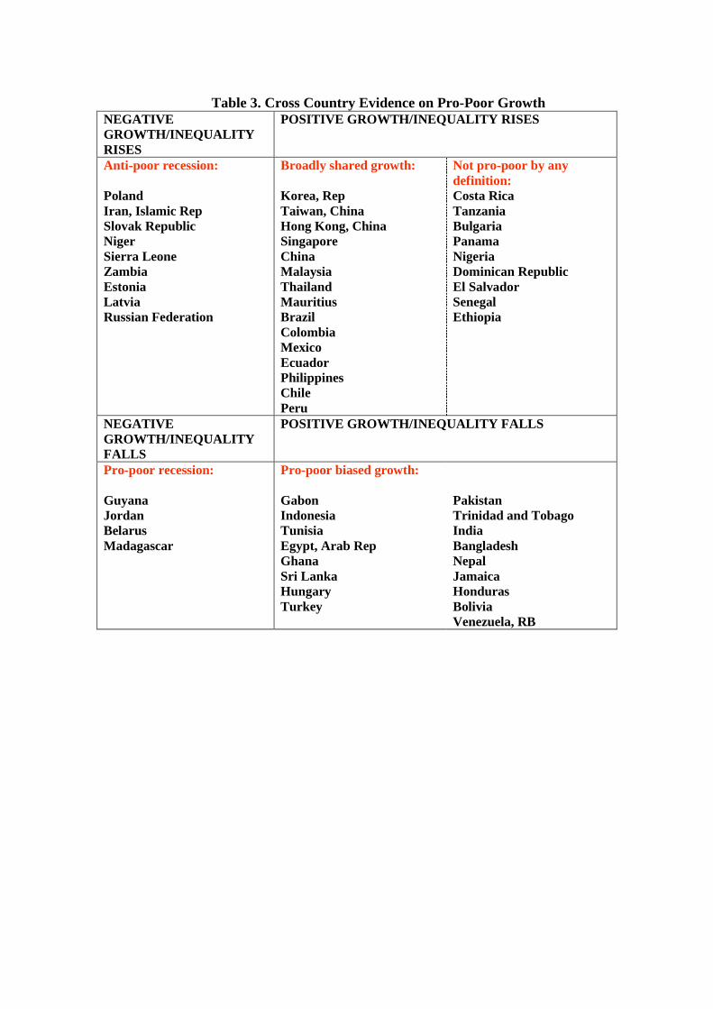
Table 3. Cross Country Evidence on Pro-Poor Growth NEGATIVE GROWTH/INEQUALITY RISES

POSITIVE GROWTH/INEQUALITY RISES

Anti-poor recession: Poland Iran, Islamic Rep Slovak Republic Niger Sierra Leone Zambia Estonia Latvia Russian Federation

Broadly shared growth: Korea, Rep Taiwan, China Hong Kong, China Singapore China Malaysia Thailand Mauritius Brazil Colombia Mexico Ecuador Philippines Chile Peru

Not pro-poor by any definition: Costa Rica Tanzania Bulgaria Panama Nigeria Dominican Republic El Salvador Senegal Ethiopia

NEGATIVE GROWTH/INEQUALITY FALLS

POSITIVE GROWTH/INEQUALITY FALLS

Pro-poor recession: Guyana Jordan Belarus Madagascar

Pro-poor biased growth: Gabon Indonesia Tunisia Egypt, Arab Rep Ghana Sri Lanka Hungary Turkey

Pakistan Trinidad and Tobago India Bangladesh Nepal Jamaica Honduras Bolivia Venezuela, RB

Figure 1. Evolution of per capita income and income of the lowest quintile: OECD countries

0

50

100

150

200

250

1970/75 75/80 80/85 85/90 90/95 95/00

YP20 Y

Figure 2. Evolution of per capita income and income of the lowest quintile: Developing

countries

020406080

100120140160180

1970/75 75/80 80/85 85/90 90/95 95/00

YP20 Y

Figure 3. Evolution of per capita income and income of the lowest quintile: East Asia and

Pacific

050

100150200

250300

350400

1970/75 75/80 80/85 85/90 90/95 95/00

YP20 Y

Figure 4. Evolution of per capita income and income of the lowest quintile: Latin America and the Caribbean

0

20

40

60

80

100

120

140

1970/75 75/80 80/85 85/90 90/95 95/00

YP20 Y

Figure 5. Evolution of per capita income and income of the lowest quintile: Middle East and North Africa

020406080

100120140160180

75/80 80/85 85/90 90/95 95/00

YP20 Y

Figure 6. Evolution of per capita income and income of the lowest quintile: Sub-

Saharan Africa

8486889092949698

100102

85/90 90/95 95/00

YP20 Y

Figure 7. Evolution of per capita income and income of the lowest quintile: South Asia

0

50

100

150

200

250

1970/75 75/80 80/85 85/90 90/95 95/00

YP20 Y