Embed Size (px)
Citation preview

1Department of Economics, University of California, Berkeley; Department of Economics,University of California, Berkeley, CEPR and NBER; and Graduate Institute of InternationalStudies, Geneva, and CEPR. This paper was prepared for the conference celebrating AssafRazin’s 60th birthday, held at Tel Aviv University, March 25-26, 2001. We thank Dennis Quinnand Andrew Warner for help with data and Anne Krueger and Dani Rodrik for comments.
2The classic illustration is that a borrower will know more than a lender about his owndesire and motivation to repay, although the point is more general. This is why banks and otherfinancial institutions play a prominent role in the modern economy: by virtue of their investmentsin monitoring technologies characterized by economies of scale and scope, they aspire to bridgegaps in the information environment that decentralized markets cannot. These observations arewidely cited in support of the notion that information asymmetries are pervasive in financial
1
When Does Capital Account Liberalization Help More than It Hurts?
Carlos Arteta, Barry Eichengreen and Charles Wyplosz1
March 2001
1. Introduction
The literature on the effects of capital mobility falls under two headings, reflecting the
traditional divide between the two branches of international economics. While work on the
effects of capital movements in models of the real economy is well advanced, due in no small part
to the important contributions of Assaf Razin, the same cannot be said of research in international
finance on the effects of capital account liberalization and international capital flows.
There are two explanations for the contrast, one having to do with theory, the other
reflecting the limitations of existing empirics. On the theoretical side there are reasons to think
that the imperfect nature of the information environment does more to complicate the effects and
consequently the analysis of financial than nonfinancial transactions. Information asymmetries are
endemic in financial markets. In particular, it is unrealistic to assume that agents on both sides of
a financial transaction have the same information.2 This is especially true of international financial

markets.
3While this conclusion is not uncontroversial, we think that the bulk of the evidence pointsin this direction. See in particular Borensztein, De Gregorio and Lee (1995), Aitken and Harrison(1999) and Bradstetter (2000).
2
transactions, in whose case information flows must travel additional physical and cultural distance.
It is well understood that these imperfections in the information environment are a distortion in
whose presence inward foreign financial investment can be welfare reducing. But the difficulty of
characterizing the information asymmetry and therefore the incidence of the distortion means that
there is no consensus on precisely when and where such immiserizing effects may take place.
In contrast, the limited conditions under which the transfer or accumulation of capital in a
real trade model is immiserizing are well understood. Brecher and Diaz-Alejandro (1977) have
pointed to import tariffs, while Brecher and Bhagwati (1991) have modeled the effects of rigid
real wages, both of which can lead foreign capital to flow into the wrong sector with immiserizing
effects. The transparency of this analysis leaves less controversy about the effects of capital
mobility in models of the real economy.
The other explanation for the contrast, and the one we pursue in this paper, is that
empirical studies of the effects of foreign direct investment (and, for that matter, trade in goods
and services) have reached more definitive conclusions than those on portfolio capital flows.
There is now a substantial body of evidence that openness to foreign direct investment is
positively associated with growth. FDI is a conduit for the transfer of technological and
organizational knowledge, suggesting that countries that welcome inward FDI should have higher
levels of total factor productivity and to enjoy faster economic growth.3 In contrast, studies of
the effects of financial capital flows are less conclusive. In part this reflects the difficulty of

3
measuring a multi-dimensional phenomenon like financial openness in an economically meaningful
way. In part it reflects the sensitivity of findings to the countries and periods considered (as we
document below).
This controversy is summarized by a pair of recent studies by Rodrik (1998b) and
Edwards (2001). Rodrik finds no correlation between capital account liberalization and growth
and comes down against the presumption that opening an economy to financial capital flows has
favorable effects. Substituting a more nuanced and presumably informative measure of capital
account liberalization, Edwards reports in contrast a strong positive effect of capital account
liberalization, one however limited mainly to high-income countries.
In this paper we seek to push this literature forward another step, by scrutinizing the
robustness of these results and addressing their implicit interpretation. We focus on the following
questions. Is there really a positive association of capital account liberalization with growth when
the former is measured in an economically meaningful way? Is it robust? Is it evident only in
certain times and places? If it is limited to high-income economies, does this reflect their more
advanced stage of financial and institutional development, which mitigates the domestic
distortions that cause capital account liberalization to have weak or even perverse effects in the
developing world? Or do the effects of capital account liberalization hinge to a greater extent on
the way it is sequenced with other policy reforms?
To anticipate our conclusions, while we find some evidence of a positive association
between capital account liberalization and growth, that evidence is decidedly fragile. The effects
vary with time, with how capital account liberalization is measured, and with how the relationship
is estimated. In our view, the evidence is insufficiently robust to support unconditional policy

4This section draws on Eichengreen (2000).
4
recommendations.
The evidence that the effects of capital account liberalization are stronger in high-income
countries is similarly fragile. There is some evidence that the positive growth effects of
liberalization are stronger in countries with strong institutions, as measured by standard indicators
of the rule of law, but only weak evidence that the benefits grow with a country’s financial depth
and development.
More important than a country’s stage of financial development, we find, is the sequencing
of reforms. Capital account liberalization appears to have positive effects on growth only in
countries that have already opened more generally. But there are significant prerequisites for
opening, most obviously a consensus in favor of reducing tariff and nontariff barriers and an
ability to eliminate macroeconomic imbalances in whose presence freeing up current account
transactions is not possible. Which of these prerequisites turns out to matter may come as a
surprise.
2. Previous Literature
The most widely-cited study of the correlation of capital account liberalization with
growth is Rodrik (1998b).4 For a sample of roughly 100 industrial and developing countries,
using data for the period 1975-1989, Rodrik regresses the growth of GDP per capita on the share
of years when the capital account was free of restriction (as measured by the binary indicator
constructed by the IMF), controlling for determinants suggested by the empirical growth literature
(initial income per capita, secondary school enrolment, quality of government, and regional

5The capital-account-openness variable is taken from line E2 (restrictions on payments forcapital transactions) of the table on exchange and capital controls in the IMF’s ExchangeArrangements and Exchange Restrictions annual.
6The results are depicted visually, using scatter plots of the partial correlation betweengrowth and the share of years when the capital account was liberalized over the period; the authordoes not report the t-statistic on the capital account liberalization variable. In fact precisely thesame result, using the same data, was published some three years earlier by Grilli and Milesi-Ferretti (1995), who report standard errors along with their point estimates.
7Quinn includes a long list of ancillary variables that have been shown to explain some ofthe cross-country variation in growth rates, drawing on Levine and Renelt (1992).
5
dummies for East Asia, Latin America and sub-Saharan Africa).5 He finds no association between
capital account liberalization and growth and questions whether capital flows enhance economic
efficiency.6
Given the currency of this article among economists, it is striking that the leading study of
the question in political science reaches the opposite conclusion. For 66 countries, using data for
the period 1960-1989, Quinn (1997) reports a positive correlation between capital account
liberalization (the change in capital account openness) and economic growth.7 That correlation is
statistically significant at standard confidence levels.
What accounts for the contrast is not clear. Quinn’s study starts earlier (it may matter that
growth in his sample period is not dominated to the same extent by the “lost decade” of the
1980s), his list of control variables is longer, and he looks at the change in capital account
openness rather than the level. Edwards (2001) has emphasized that Quinn uses a more nuanced
and therefore more informative measure of capital-account liberalization. For 58 countries over
the period 1950 to 1994 and an additional 8 countries starting in 1954, Quinn distinguishes 7
categories of statutory measures. Four are current account restrictions, two are capital account

6
restrictions, and one measures international agreements like OECD membership constraining the
ability of a country to limit exchange and capital flows. For each of these categories, Quinn codes
the intensity of controls on a two-point scale (in half point increments from 0 to 0.5, 1, 1.5, 2,
with 0 denoting most intense and 2 denoting no restriction), producing an overall index of current
and capital account restrictions that ranges from 0 to 14 and a capital account restrictions
measure that ranges from 0 to 4.
Also important may be that Quinn’s country sample is different; in particular, he considers
fewer low-income developing countries. The recent literature gives reason to think that the
effects of capital account liberalization vary with financial and institutional development.
Removing capital controls may be welfare and efficiency enhancing only when major
imperfections in the information and contracting environment are absent; this is an implication of
the theory of the second best. Portfolio capital inflows stimulate growth, the argument goes, only
when markets have developed to the point where they can allocate finance efficiently and when
the contracting environment is such that agents must live with the consequences of their
investment decisions. The Asian crisis encouraged the belief that countries benefit from removing
controls only when they first strengthen domestic markets and institutions generally; thus, we
should expect a positive association with growth only when prudential supervision is first
upgraded, the moral hazard created by an excessively generous implicit and explicit financial
safety net is limited, corporate governance and creditor rights are strengthened, and transparent
auditing and accounting standards and efficient bankruptcy and insolvency procedures are
adopted. While these institutional prerequisites are difficult to measure, there is a presumption
that they are most advanced in high-income countries. This is one way of understanding how

8The evidence is not overwhelming: Alesina, Grilli and Milesi-Ferretti report a positivecoefficient that differs significantly from zero at standard confidence levels in one of fourregressions. Moreover, the specification in question does not control for initial per capita income;once it is added, the correlation in question dissolves. Bordo and Eichengreen (1998) explicitlycompare industrial and developing countries, and report weak evidence that controls have apositive impact on growth in the industrial countries, and a negative impact on growth indeveloping countries, although the operative word is “weak.”
9Quinn (2000) uses a very different methodology to address this question but reaches asimilar conclusion. He estimates bivariate VARs using growth rates and his measures of capitalaccount liberalization, individually for a large number of middle- and low-income countries. Hefinds scant evidence that capital account liberalization has had a positive impact on growth in thepoorest countries, but some positive evidence for middle-income countries, especially those that
7
Alesina, Grilli and Milesi-Ferretti (1994) find evidence of a positive association between capital
account liberalization and growth -- their sample is limited to 20 high-income countries -- when
Grilli and Milesi-Ferretti (1995) find a negative association in a sample dominated by developing
countries.8
Edwards (2001) addresses the hypothesis that capital account liberalization has different
effects in high- and low-income countries. Using Rodrik’s controls but Quinn’s measure of the
intensity of capital account restrictions in 1973 and 1988, he finds that liberalization boosts
growth in the 1980s in high-income countries but slows it in low-income countries. (The dummy
variable for capital-account openness enters negatively, in other words, while the interaction
between capital-account openness and per capita income enters positively.) Edwards shows
further that the significance of capital controls evaporates when the IMF index used by Rodrik is
substituted for Quinn’s more differentiated measure. Thus, it is tempting to think that the absence
of an effect in previous studies is a statistical artefact. And there is some suggestion that capital
account liberalization is more beneficial in more financial and institutionally developed
economies.9

have other characteristics likely to render them attractive to foreign investors.
10Kraay uses the ratio of M2 to GDP and the ratio of domestic credit to the private sectorrelative to GDP as ex ante proxies for the level of financial development, and one minus theaverage number of banking crises per year as an ex post indicator of financial strength. As anindicator of the strength of bank regulation, he uses authorization for banks to engage innontraditional banking activities such as securities dealing and insurance. And to capture thebroader policy and institutional environment, he uses a weighted average of fiscal deficits andinflation, the black market premium, and indices of corruption and the quality of bureaucracy.
8
But do these differences really reflect the level of financial and institutional development?
Kraay (1998) is the one direct attempt to test the hypothesis that the effects of capital account
liberalization depend on the strength of the financial system, the effectiveness of prudential
supervision and regulation, and the quality of other policies and institutions, rather than seeking to
infer this from differences between industrial and developing economies.10 The results are not
encouraging: the interaction of the quality of policy and institutions with financial openness is
almost never positive and significant, and, it is sometimes significantly negative. But while these
findings are intriguing, their generality is an open question; the other work reviewed in this section
raises questions about whether they are sensitive to country sample, specification, and in
particular how financial openness is measured. To the extent that capital account liberalization
has different effects on growth in high- and low-income countries, the reasons for the contrast
remain unclear.
3. Basic Results
In this section we scrutinize the claim that the effects of capital account liberalization
differ between high- and low-income economies -- and, specifically, that they are positive in the
former but not the latter.

11In contrast, the IMF measure of capital account openness bears no association togrowth, as mentioned above.
12Quinn has also made available his 1958 estimates to other investigators, but these areirrelevant to the current exercise.
13Including only the 1988 value but instrumenting it using the 1973 index, as Edwardsdoes in some of his analysis, does not obviously solve this problem.
9
Our point of departure is Edwards’ model. Edwards regresses economic growth in the
1980s (approximately the same period considered by Rodrik) on the decennial average investment
rate, years of schooling completed by 1965 (as a measure of human capital), the log of real GDP
per capita in 1965 (as a measure of the scope for catch-up), and Quinn’s index of capital account
openness. He reports that this measure of capital account openness has a positive and generally
significant effect on growth. Moreover, when capital account openness is entered both on its own
and interacted with per capita incomes, the first coefficient is negative and the second positive.11
The inflection point where the effect of capital account openness becomes positive coincides with
the per capita incomes achieved by the 1980s by such relatively-advanced emerging markets as
Hong Kong, Israel, Mexico, Singapore and Venezuela.
Four aspects of Edwards’ data and specification are worthy of comment. First, while he
uses annual data spanning the 1980s for his other variables, Edwards has Quinn’s measure of
capital account openness for only 1973 and 1988.12 The 1973 value is arguably too early to have
a first-order effect on growth in the 1980s, while the 1988 value is arguably too late.13 Similarly,
the difference in the level of openness in 1973 and 1988 may tell us how policies toward the
capital account changed in the 1970s and 1980s, but these two snapshots are equally compatible
with the possibility that the change took place before the beginning of the sample period or at its

14Edwards’ two sets of estimates use, alternatively, the Quinn index for 1988 and thedifference between Quinn’s 1973 and 1988 values.
15In addition, heavy weights on high income countries, which were also the relatively fastgrowing countries in some of the subperiods we consider (see below), increases the danger offinding a correlation between capital account liberalization and growth because of reversecausality (insofar as the high-income countries were the ones most likely to open the capitalaccount).
16In addition, Edwards derives his results from estimates of a two-equation system, wherethe dependent variables are GDP growth and TFP growth and the list of independent variables isthe same across equations. Since the second dependent variable is derived (in part) from the first,errors in GDP growth are likely to produce (positively correlated) errors in TFP growth. Whenthe correlation between the error terms in the two equations is taken into account via systemestimation, the econometrician may therefore obtain a spuriously strong correlation with the
10
end, two scenarios which presumably imply very different effects.14
Second, Edwards weights his observations by GDP per capita in 1985. We worry that
placing an especially heavy weight on rich countries with well-developed institutions biases the
case in favor of finding a link between capital account liberalization and growth, since these are
the countries in which such an effect is most plausibly present.15
Third, Edwards instruments his measure of capital account liberalization with a vector of
concurrent and lagged economic, financial and geographical variables. While we are sympathetic
to the idea that policies toward the capital account may be affected by as well as affect growth,
useful instruments -- variables that are exogenous but also correlated with capital account
liberalization -- are hard to come by. In particular, we are skeptical that geographic variables are
usefully correlated with capital account liberalization (although previous work has shown that
they importantly influence the level of income and/or the rate of growth), and we would question
whether the economic and financial variables invoked in this context are properly regarded as
exogenous with respect to the policy.16

independent variables.
17Details on the data underlying this and subsequent tables can be found in the dataappendix.
18We also augmented the list of controls to include distance from the equator, since thisvariable is included among the instrumental variables we experiment with below, and others (e.g.Rodrik 2000) have argued that it has an independent impact on economic growth. While thisvariable often enters with a significant coefficient, adding it only reinforces our results (as we
11
Fourth, neither Edwards nor other contributors to this literature include competing
measures of economic openness and the macroeconomic policy regime. Typically, countries that
open the capital account also open their economies to other transactions (for example, they will
have reduced tariff and nontariff barriers to trade). In the absence of measures of these other
policies, it is not obvious that the index of capital account openness is picking up the effects of
financial openness as opposed to the openness of, say, the trade account. Similarly, governments
may wait to open the capital account until they have first succeeded in eliminating macroeconomic
imbalances that would precipitate capital flight through newly-opened channels; a positive effect
of capital account liberalization on growth may reflect the growth-friendly effects of
macroeconomic stabilization, in other words, rather than international financial policies per se.
We show some “Edwards regressions” in Table 1 (single equation estimates for the 1980s,
with and without weights, using the 1988 level of the Quinn index and, also following Edwards,
the change in Quinn’s index between 1973 and 1988).17 The controls -- the investment ratio,
human capital, 1965 per capita GDP -- are consistently significant and have their anticipated signs.
In the unweighted least squares regressions, both the level of capital account openness in 1988
and its change between 1973 and 1988 enter with positive coefficients, but only the latter differs
from zero at the 95 per cent level.18 In the weighted least squares regressions, the converse is

explain below).
19These regressions are not reported but are available from the authors on request.
20The coefficient on the level of the Quinn index by itself (column 3) is negative butinsignificantly different from zero, lending no support to the hypothesis that liberalization damagesgrowth in low-income countries. It is however the case that we can reject the null that bothcoefficients (that on the level of the Quinn index and the interaction term) are zero at the 95 percent confidence level.
12
true: the level of capital account openness differs from zero at the 95 per cent confidence level,
but the change does not. There is some evidence, then, of a positive association between capital
account liberalization and growth, although it is decidedly fragile.
Following Edwards, we re-estimated these equations substituting the binary measure of
capital-account restrictions based on information in the IMF’s Exchange Arrangements and
Exchange Restrictions annual, constructing this variable as the share of years in the sample period
when the capital account was open. As in his analysis, none of the coefficients on this variable
approached significance at conventional confidence levels.19 This is support for Edwards’ first
point, that the growth effects of capital account liberalization are more evident when the latter is
proxied by the (presumably more informative) Quinn measure.
When we interact the Quinn measure with per capita GDP in 1980 (that being the start of
Edwards’ sample period), we find little support for the notion that capital account liberalization
has different effects in high- and low-income countries. In the unweighted least squares
regressions (columns 1-4 of Table 1), the coefficient on the interaction of the Quinn index and
1980 per capita GDP is positive and significantly different from zero at the 95 per cent confidence
level, as if the effects of liberalization are larger in high-income countries.20 But we find no such
effect in the weighted least squares regressions or when we measure capital account liberalization
21The results are essentially the same, although a little weaker, when we use membership inthe OECD in place of per capital GDP when constructing the interaction term. In the weightedleast squares regressions, all interaction terms are insignificantly different from zero atconventional confidence levels.
22Edwards’ key results -- those obtaining nonlinear effects for capital account liberalization(negative at low levels of per capital income, positive at high levels) -- are derived using three-stage least squares.
13
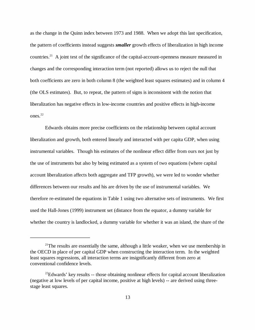
as the change in the Quinn index between 1973 and 1988. When we adopt this last specification,
the pattern of coefficients instead suggests smaller growth effects of liberalization in high income
countries.21 A joint test of the significance of the capital-account-openness measure measured in
changes and the corresponding interaction term (not reported) allows us to reject the null that
both coefficients are zero in both column 8 (the weighted least squares estimates) and in column 4
(the OLS estimates). But, to repeat, the pattern of signs is inconsistent with the notion that
liberalization has negative effects in low-income countries and positive effects in high-income
ones.22
Edwards obtains more precise coefficients on the relationship between capital account
liberalization and growth, both entered linearly and interacted with per capita GDP, when using
instrumental variables. Though his estimates of the nonlinear effect differ from ours not just by
the use of instruments but also by being estimated as a system of two equations (where capital
account liberalization affects both aggregate and TFP growth), we were led to wonder whether
differences between our results and his are driven by the use of instrumental variables. We
therefore re-estimated the equations in Table 1 using two alternative sets of instruments. We first
used the Hall-Jones (1999) instrument set (distance from the equator, a dummy variable for
whether the country is landlocked, a dummy variable for whether it was an island, the share of the

23This was true both of the individual coefficients and, when Quinn openness was enteredin levels and interacted with per capital GDP, of the pair. That is, the relevant F-statistic did notlead us to reject the null that the two coefficients were effectively zero. Note that this is wherethe decision of whether or not to include distance from the equator as an explanatory variable forgrowth could matter. It is reassuring, therefore, that adding it to the list of independent variablesaltered none of the results reported here.
24This is our reading of the abbreviations in the instrument list at the bottom of his Table10.
14
population speaking English, and the share of the population speaking a major European
language). None of the measures of capital account liberalization -- its level or change, entered by
itself or interacted with per capital GDP -- entered with a coefficient that approached significance
at standard confidence levels.23 While these instruments are plausibly exogenous, either they are
not usefully correlated with capital account liberalization or the latter in fact has no independent
impact on growth.
The second set of instruments is our attempt to replicate those used by Edwards: whether
the capital account was open or closed in 1973, the ratio of liquid liabilities to GDP in 1970 and
1975, distance to the equator, and a dummy variable for OECD countries.24 The results, in Table
2, differ sharply from before. The coefficient on the Quinn index in 1988 is still positive when
entered on its own, albeit somewhat less well defined than in Table 1. However, when the
interaction of capital account openness and per capita GDP is added, the coefficient on the level
of the Quinn index turns negative (though insignificant), while the interaction term is positive and
significantly different from zero at the 95 per cent confidence level. This is very close to
Edwards’ result. However, this pattern obtains only when we enter capital account openness in
levels (rather than changes between 1973 and 1988) and only when we estimate by unweighted
least squares (as opposed to applying per capita GDP weights). And it is sensitive to the choice

25In addition, we worry about the validity of the instruments, specifically whether laggedliberalization and financial depth, which move slowly and are correlated with current liberalizationand financial depth, are in fact capturing the exogenous component of these international financialpolicies. See the discussion above.
15
of instrumental variables. For example, the one coefficient on the interaction term that was
previously significantly positive goes to zero when either financial depth or lagged openness (or,
for that matter, both) is dropped from the instrument list but the other instrumental variables are
retained.25
Thus, we confirm that an analysis of developing- and industrial-country experience in the
1980s yields somewhat more favorable results for the association of capital-account openness and
growth when capital-account policies are measured using Quinn’s index rather than the IMF
measure. The evidence that this effect is stronger in high-income countries turns out to be
extremely sensitive to specification and estimation.
4. Sensitivity Analysis
In this section we subject these results to two forms of sensitivity analysis. First, we
adjust the timing of the dependent and independent variables in order to better identify the effects
of capital account policies. Second, we compare the effects of capital account liberalization in
different periods.
Recall that Edwards uses Quinn’s measure of capital-account openness in 1973 and 1988.
If capital account liberalization has a significant impact on growth, this should be most evident in
the immediately succeeding years. Having analyzed growth in the 1980s as a way of rendering
our results as directly comparable as possible to those of Edwards and other investigators, we

26In principle, it would be possible to extend this sample beyond 1992 using data fromother sources. But given the far-reaching changes in capital-account restrictions that occurred inthe 1990s, our measure of the structure of capital controls, circa 1988, would then capture littleof the reality of capital-account policies in the last subperiod. Since we do not have Quinn-likedata on the capital-account regime in the 1990s, we concluded that it makes sense to stick with asample that ends in 1992.
27We thank Dennis Quinn for sharing these data with us.
28We report results using only the Quinn measure of openness, since when we substitutethe IMF measure we obtain uniformly insignificant effects. We concentrate on unweightedregressions throughout. The use of weights and instrumental variables alters our results onlyslightly: the coefficients tend to be slightly less well determined, although the pattern of signsremains the same.
16
now focus on the effects of capital account liberalization in the years immediately following those
for which we have Quinn’s capital account restrictions data: 1973 and 1988. The obvious
stopping point for the period starting in 1973 is 1981, the eve of the Mexican debt crisis and the
“lost decade” of the 1980s, when capital flows were subdued and their growth effects were
plausibly different. Our second cross section (starting in 1988) ends in 1992, since that is when
our data, drawn from the Penn World Tables Mark 5.6a, end.26 This leaves a gap in the mid-
1980s. Fortunately, we were also able to obtain Quinn’s measure of capital account openness for
1982.27 Thus, we can analyze three cross sections covering the periods 1973-81, 1982-87, and
1988-92. We also pool the three cross sections. The pooled results will reassure readers worried
that conditions during one or more of our periods were special (“1982-87 is unrepresentative
because it is dominated by the debt crisis,” for example). Aggregating across periods limits the
danger that our results are being driven by period-specific effects.
The results are in the Table 3. In the first four columns we enter capital account openness
in levels; in the second four we also interact it with per capita GDP.28 Given the questions about

29Investment retains is consistently positive effect on growth, although the effects ofhuman capital are somewhat weaker than before. The catch-up effect is weak in both the secondand third periods, reflecting the heavy impact of the debt crisis of low- and middle-incomedeveloping countries starting in 1982 and their delayed post-1987 recovery.
17
instrumentation raised in the last section, we estimate the equations by ordinary least squares.
The results remain generally plausible.29 When entered exclusively in levels, the Quinn
measure of financial openness is positively associated with growth in all three periods, but only in
the third of these, 1988-92, is the effect significant at anything approaching conventional
confidence levels. The coefficient is smallest in the period starting in 1982, when capital flows
were depressed by the debt crisis, and largest in the post-1987 period, the year of the Brady Plan
after which large scale portfolio capital flows resumed. But when we pool the three cross
sections (adding fixed effects to differentiate the subperiods), the coefficient on capital account
liberalization differs from zero at the 95 per cent confidence level. This is the strongest evidence
so far of a positive association of capital account liberalization and growth, although it is clear
that this result is heavily driven by one of our cross sections.
But there is still scant evidence of a stronger growth effect in high-income countries. We
obtain a significant positive coefficient on the interaction term only for the post-1982 years.
Perhaps capital account liberalization worked its magic more powerfully on high-income countries
in these years. Alternatively, it may simply be that high-income (OECD) countries with open
capital accounts were less affected by the debt crisis of the 1980s than developing countries with
open capital account that had grown heavily dependent on foreign borrowing. Whether this in
fact tells us anything about the differential effects of capital account liberalization in different
developing countries is unclear.

30Again, for details on this and the other variables used in the analysis, see the dataappendix.
18
In the pooled sample, the coefficient on the interaction term is indistinguishable from zero.
However, the coefficient on capital account liberalization in levels continues to enter positively
and differs from zero at the 90 per cent confidence level. Again, however, this result appears to
be driven by the strong positive association in the post-1987 period.
Thus, more data and appropriate timing of the variables continue to provide indications a
positive association of capital account liberalization with growth. However, that effect is robust
only for the most recent period, that is to say, for the post-Brady Plan years. There is less
evidence to this effect for earlier periods, whether these are the years of syndicated bank lending
to developing countries or of the developing country debt crisis. Moreover, we find little support
for the view that capital account liberalization has more favorable effects in high- and middle-
income emerging markets than in poorer developing countries.
5. Do These Patterns Reflect Stages of Financial and Institutional Development?
We now ask whether the different effects of capital account liberalization in high- and
low-income countries in fact reflect their different stages of financial and institutional
development. To this end, we interact Quinn’s index not with per capita GDP but with financial
depth (proxied by the ratio of liquid liabilities to GDP) and institutional strength (the
International Country Risk Guide’s index of law and order).30
The results are in Table 4, the first four columns for financial depth (post 1973, post 1982,
post 1988, and pooled, reading left to right), the last four for law and order. Those for financial

31Again, estimating these equations by instrumental variables changed nothing.
32At the 90 and 95 per cent levels, respectively.
33One of the coauthors is reminded of all the money deposited in Swiss banks bydepositors from countries that rate low according to the law-and-order index and with porouscapital accounts.
34We also fail to reject the null that the two coefficients are jointly zero at conventionalconfidence levels.
19
depth are unpromising: none of the coefficients in question is significant individually or as a pair.31
The results for the interaction between capital account openness and rule of law are more
promising. In the first subperiod (1973-81) we obtain a negative coefficient on capital account
openness in levels and a positive coefficient on the interaction term; the latter differs from zero at
the 95 per cent confidence level. The interpretation is that capital account liberalization has no
effect in countries with weak contract and law enforcement but a positive effect in those with
stronger ones. The results for the second subperiod (1982-87) are more striking still: both terms
again enter with the expected signs, and both now differ from zero at conventional confidence
levels.32 According to this column at least, capital account liberalization hinders growth when a
country rates low on the law-and-order index but helps when it rates high.33 In comparison, the
results for the most recent subperiod (1988-92) are disappointing: neither coefficient enters with
its expected sign, and neither differs significantly from zero at standard confidence levels.34
The results for the pooled sample reflect these contrasting subsample results. The
coefficient on the level of Quinn openness is zero, but the coefficient on the interaction term is
positive and significant at the 90 (but not the 95 per cent) confidence level.
Thus, we find scant support for the hypothesis that the effects of capital account

35See for example Edwards (1994) and Johnston (1998).
20
liberalization reflect a country’s stage of financial development. There is more support for the
idea that the effects vary with the effectiveness of law and order, but the evidence is not
overwhelming.
6. Sequencing
It could be that we are not capturing the full impact of capital account liberalization on
growth because we are not controlling efforts to coordinate external financial opening with other
liberalization measures. There is a large literature on sequencing that suggests that capital
account liberalization initiated before the current account is opened can have strongly
distortionary effects (see McKinnon 1991). If trade barriers continue to protect an uneconomical
import-competing sector, foreign capital will flow there, attracted by rents and artificially inflated
profits. Since the country has no comparative advantage in those activities, actually devoting
more resources to import-competing production can be growth and welfare reducing. In
particular, the cost of the resources that the country utilizes to service the foreign finance may
exceed the cost of capital, reducing domestic incomes as well as starving other sectors of inputs
to growth (Brecher and Diaz-Alejandro 1977). Similarly, the literature on the sequencing of
financial liberalization measures cautions that it can be counterproductive to open the international
accounts before domestic macroeconomic imbalances have been eliminated; the main effect will
then be to provide avenues for capital flight.35 If domestic financial markets are repressed, capital
account liberalization allows savers to flee the local low-interest rate environment in favor of
higher returns abroad. For all these reasons, capital account liberalization when macroeconomic

36We thank Andrew Warner for providing these data.
37Rodriguez and Rodrik (1999) note that the state monopoly of major exports variable isderived from a World Bank index of the degree of distortions caused by export marketing boardsand is positive only for sub-Saharan African countries, whose growth performance wasparticularly disappointing in the sample period. Since there are only two sub-Saharan Africancountries in our (much smaller) sample, it is not plausible in our case that this is the properinterpretation of the results we obtain when we use the Sachs-Warner openness measure.
21
policy is seriously out of balance is a recipe for disaster.
To capture these qualifications, we added the interaction between capital account
openness, as measured by Quinn, and nonfinancial openness, as measured by Sachs and Warner
(1995).36 This is analogous to our earlier tests of the idea that the effects of capital account
openness are contingent on financial depth and institutional development, but now the hypothesis
is that they are contingent on the absence of trade and macroeconomic distortions. The Sachs-
Warner index classifies a country as open if none of the five following criteria holds: the country
had average tariff rates higher than 40 per cent, its nontariff barriers covered on average more
than 40 per cent of imports, it had a socialist economic system, the state had a monopoly of major
exports, and its black market premium exceeded 20 per cent. The first four criteria should allow
us to test the notion that capital mobility is counterproductive for an economy whose trade is
highly restricted and distorted.37 The fifth is an indicative of macroeconomic policies and
conditions inconsistent with a country’s administered exchange rate; it should allow us to test the
hypothesis that capital account liberalization is counterproductive if implemented before a country
has eliminated macroeconomic imbalances.
The results are in Table 5, columns 1-4. The specification is analogous to that of Table 3
but for the addition of the interaction of the Sachs-Warner dummy with Quinn openness. We find

38Only in the first subperiod, for 1973-81, is its coefficient not significantly greater thanzero at the 95 per cent confidence level.
22
a strong positive effect of this interaction term, almost irrespective of period.38 In the pooled
sample, it differs from zero at the 99 per cent confidence level. This suggests that capital account
openness stimulates growth when a country has eliminated major trade distortions and
macroeconomic imbalances, but not otherwise.
We undertook some sensitivity analyses of this finding. We estimated the equations by
weighted as well as unweighted least squares. We used Edwards’ instrumental variables. We
searched for and dropped outliers. We added the interaction between financial depth and financial
openness and the interaction between law and order and financial openness as in Table 4 above.
None of these changes weakened the result.
The one change that made a difference was adding Sachs-Warner openness in levels. We
show the result of doing so in columns 5-8 of Table 5. The three openness measures (Sachs-
Warner openness, Quinn capital account openness, and their interaction) are highly correlated,
creating problems of multicolinearity. Only in the pooled sample is there much hope of
distinguishing their effects. There, Sachs-Warner openness and Quinn openness both have
(positive) coefficients that differ from zero at the 90 per confidence level, while their interaction is
insignificant. This points less to the importance of sequencing than to separate, non-
interdependent effects on growth of both Sachs-Warner and capital account openness. But
multicolinearity makes it difficult to know which interpretation is appropriate. While the relevant
F-test allows us to reject the null that the levels of both Sachs-Warner openness and Quinn
openness are zero, consistent with the separate, non-interdependent-effects interpretation, it also

39As noted above, Sachs-Warner openness involves two additional criteria -- whether acountry had a socialist economic system and the state had a monopoly of major exports -- whichare likely to matter importantly for certain countries. We return to this point below.
40This is similar to the approach taken by Rodriguez and Rodrik (1999), who find ingrowth regressions covering a longer period that it is the black market premium in which most ofthe explanatory power resides.
41Note that the Barro-Lee tariff and nontariff data do not vary with time. The same is trueof the Sachs-Warner index (which makes use of the Barro-Lee measures), aside from a fewselected changes imposed by its architects.
23
allows us to reject the null that Quinn openness and the interaction of Sachs-Warner openness
with Quinn openness are both zero, consistent with the sequencing interpretation.
It turns out that we can get a better handle on which interpretation is more plausible by
analyzing whether absence of a favorable impact on growth in countries that are closed according
to the Sachs-Warner measure reflects distortionary trade policies or distortionary macroeconomic
policies. We do so by breaking Sachs-Warner openness up into its two principal components, one
reflecting the prevalence of tariff and nontariff barriers (distortionary trade policies), and the other
reflecting the size of the black market premium (an indicator of macroeconomic imbalances).39 If
it is the interaction term involving the black market premium that matters, then we can say that it
is the elimination of macroeconomic imbalances that is the essential prerequisite for capital
account liberalization to have positive growth effects, a la McKinnon. If, on the other hand, it is
the interaction involving tariff and nontariff barriers that is significant and important, we can say
that it is the elimination of trade-related distortions that is key, a la Brecher and Diaz-Alejandro.40
We measured tariff and nontariff barriers using the data of Barro and Lee (1994), which
conveniently are also utilized by Sachs and Warner.41 For the black market premium, we
constructed three alternative measures. First, we created a dummy variable which equaled unity if

42We refer to this in Table 6 as “black market premium 1.”
43This is “black market premium 2.” We divide the premium by 100 so that thecoefficients on this variable are scaled the same as for “black market premium 1.”
44Denoted “black market premium 3.” Again, we divide this measure by 100 to make it ascomparable as possible with “black market premium 1.”
45We see the same pattern when we consider the individual subperiods, although thecoefficients, predictably, are less well defined than when we pool the data. We discuss thesubperiod results later in this section.
24
the black market premium was less than 20 per cent.42 While this follows Sachs and Warner as
closely as possible, it does not use all the available information. We therefore also defined an
alternative measure, 100 per cent minus the black market premium.43 While this contains more
information, the results obtained when using it are more likely to be dominated by a handful of
extreme observations. This led us to create a third version of the variable, which truncated 100
per cent minus the black market premium at zero on the downside.44
It turns out that it is the interaction term between capital account openness and the black
market premium that most consistently matters. Columns 1-3 of Table 6 display pooled
regressions using the three alternative measures of the premium. The interaction with the black
market premium is positive, and its coefficient is significantly greater than zero at the 90 per cent
confidence level, regardless of how that premium is defined and measured. The evidence that
trade openness is a prerequisite for capital account openness to stimulate growth is less robust;
while the coefficient on the interaction with tariff and Barro and Lee’s trade openness measure is
consistently positive, it approaches significance at conventional confidence levels in only one of
the three regressions.45
Again, we attempted to confirm the robustness of this finding. We added interaction

46These are discussed in the next paragraph. To conserve space, we report only the resultsfor “black market premium 1." Those using the other measures of the black market premium areessentially identical.
25
terms involving financial depth and law and order, as in Table 4. We ran regressions using
weighted as well as unweighted observations. In each instance the results were essentially
unchanged. The one sensitivity analysis that mattered was adding Sachs-Warner openness in
levels. The results are in the last three columns of Table 6. Evidently, the two measures of
external policy with the most robust, consistent effects on growth are (i) Sachs-Warner openness
and (ii) the interaction of the black market premium with capital account openness. In other
words, there is strong evidence, as before, that countries that open externally in the sense of Sachs
and Warner grow faster, other things equal. In addition, however, countries that open the capital
account also grow faster but only if they first eliminate any large black market premium. Capital
account openness has favorable effects, it would appear, only when macroeconomic imbalances
leading to inconsistencies between the administered exchange rate and other policies have first
been eliminated.
Table 7 reports a selection of subperiod results.46 These reveal that the positive effect of
capital account openness on growth, contingent on the absence of a large black-market premium,
is driven by the 1982-87 subperiod. In addition, previously (in Tables 3-5) the coefficient on
capital account openness in levels was either positive or zero. There was no evidence, in other
words, that capital account openness was bad for growth in countries with underdeveloped
financial markets, weak institutions, severe macroeconomic imbalances, or closed current
accounts. Now the coefficient on the level of Quinn’s index is strongly negative in 1982-87, as if
countries with significant trade distortions and large black market premia grew more slowly if

26
they ill advisedly opened their capital accounts. That this effect is most evident in the debt-crisis
years 1982-87 may be telling us that countries that poorly sequenced capital account liberalization
suffered the most devastating effects of the curtailment of capital flows; they suffered a severe
debt overhang and an intractable transfer problem when the debt crisis struck. It may be that
improper sequencing does not actually damage growth so long as international capital markets are
flush with funds, but that it can result in serious damage if lending suddenly dries up.
7. Conclusion
Economic theory creates a strong presumption that capital-account liberalization has
favorable effects on growth. Yet the accidents and disappointments suffered by countries
liberalizing their international financial transactions remind us that reality is more complex than
theory. The quest for guidance is not helped by the fact that the data do not speak loudly. Some
analysts have rejected the hypothesis that there is a positive association between capital account
liberalization and growth, while others have reported evidence of a favorable effect.
The idea that the effects of capital-account liberalization are conditioned by a country’s
stage of financial and institutional development similarly has intuitive appeal. Not only are there
good theoretical reasons to think that this might be the case, but it could be the failure of previous
investigators to incorporate this idea that accounts for the weak and inconsistent results of their
econometric studies. Yet our tests of the hypothesis are only weakly supportive. We find no
evidence that the effects of capital account liberalization vary with financial depth, but somewhat
more evidence that its effects vary with the rule of law.
In contrast, we find somewhat more evidence of a correlation between capital account

27
liberalization and growth when we allow the effect to vary with other dimensions of openness.
There are two interpretations of this finding, one in terms of the sequencing of trade and financial
liberalization, the other in terms of the need to eliminate major macroeconomic imbalances before
opening the capital account. By and large, our results support the second interpretation. While
trade openness has a positive impact on growth, the effect of capital account openness is not
contingent on openness to trade. Rather, it is contingent on the absence of a large black market
premium -- that is to say, on the absence of macroeconomic imbalances. In the presence of such
imbalances, capital account liberalization is as likely to hurt as to help.
If we are right, ours is the first systematic, cross-country statistical evidence that the
sequencing of reforms shapes the effects of capital account liberalization. But our analysis also
suggests that this result may be period-specific: the evidence that sequencing matters is more
robust in the 1980s than in the 1970s or 1990s. If this investigation has taught us one thing, it is
not to oversell such results. Considerable additional analysis is required to establish the generality
of such findings.

28
Data Appendix
Our sample includes the following 61 countries: Argentina, Australia, Austria, Belgium,Bolivia, Brazil, Canada, Chile, Colombia, Costa Rica, Denmark, Dominican Republic, Ecuador,Egypt, El Salvador, Finland, France, Germany, Ghana, Greece, Guatemala, Haiti, Honduras,Hong Kong, India, Indonesia, Iran, Iraq, Ireland, Israel, Italy, Jordan, Korea, Liberia, Malaysia,Mexico, Myanmar, Netherlands, New Zealand, Nicaragua, Norway, Pakistan, Panama, Paraguay,Peru, Philippines, Portugal, Singapore, South Africa, Spain, Sri Lanka, Sweden, Switzerland,Syrian Arab Republic, Thailand, Tunisia, Turkey, United Kingdom, United States, Uruguay, andVenezuela.
Dependent Variable: Rate of growth of real GDP per capita, defined as the first difference ofthe log of real GDP per capita in constant dollars at 1985 international prices. Source: PennWorld Tables, Mark 5.6a.
Controls:
C Real investment share of GDP (%) at 1985 international prices. The variables used inthe regressions are averages of this variable over particular periods of time, as noted in thetext and tables. Source: Penn World Tables, Mark 5.6a.
C Average years of schooling of the population over 15 years of age. This variable isavailable quinquennially for the years 1960-1990. For Tables 1 and 2, the 1965 value wasused. For the other tables, the values for 1970 (for the 1973 cross-section), 1980 (for the1982 cross-section), and 1985 (for the 1988-cross section) were used. (Given lack of1970 data for Egypt, the value for 1975 was used in the 1973 cross-section for thiscountry.). Source: Barro-Lee data set (see Barro and Lee 1996).
C Log of GDP per capita in constant dollars (chain index) at 1985 international prices. Thevalue for 1965 is used in Tables 1 and 2. In the other tables, the value for the beginning ofthe corresponding period was used. Source: Penn World Tables, Mark 5.6a.
Financial and Institutional Development:
C Financial depth, defined as the ratio of liquid liabilities to GDP (%). Values at thebeginning of the period were used. Source: Beck, Demirguc-Kunt, and Levine (1999).
C Law and order index, which ranges from zero to six, where a higher value represents abetter institutional framework. Source: International Country Risk Guide. Since thisindex starts only in 1984, we use the 1984 value for 1973 and 1981.
Financial Openness:

29
C Quinn index, which ranges from zero to four in increments of 0.5, where a higher valuerepresents a more open capital account. Values for 1973, 1982, and 1988 are available. The value for 1988 and the difference between the 1973 and 1988 values were used inTables 1 and 2. In the other tables, the value for the beginning of the correspondingperiod was used. Source: personal correspondence with Dennis Quinn.
C IMF capital account openness dummy, constructed from line E2 (“restrictions onpayments for capital transactions”) of the IMF Annual Report of Exchange Arrangementsand Exchange Restrictions, various issues. The variable used was the share of years in thesample period when the capital account was open. Source: IMF.
Non-Financial Openness:
C Sachs-Warner openness dummy, defined as a binary variable equal to one if none of thefive following criteria holds: the country had average tariff rates higher than 40 per cent,its nontariff barriers covered on average more than 40 per cent of imports, it had asocialist economic system, the state had a monopoly of major exports, and its blackmarket premium exceeded 20 per cent. Source: Sachs and Warner (1995), via personalcorrespondence with Andrew Warner.
C Barro-Lee trade openness dummy, defined as binary variable equal to one if a countrydid not have average tariff rates higher than 40 per cent and its nontariff barriers did notcover on average more than 40 per cent of imports. Source: Barro and Lee (1994).
C Black market premium, defined as per cent premium over the official exchange rate. Source: personal correspondence with Andrew Warner.
Instruments:
C Liquid liabities to GDP (as defined above), for 1970 and 1975. Source: Beck,Demirguc-Kunt, and Levine (1999).
C Distance to the equator. Source: Hall and Jones (1999).
C OECD membership dummy. Source: World Development Indicators, World Bank.
C Language variables, corresponding to: (a) the fraction of the population speakingEnglish, and (b) the fraction of the population speaking one of the major languages ofWestern Europe: English, French, German, Portuguese, or Spanish. Source: Hall andJones (1999).
C Landlocked nation dummy. Source: Andrew Rose’s website.

30
C Island nation dummy. Source: Andrew Rose’s website.

31
References
Aitken, Brian J. and Ann E. Harrison (1999), “Do Domestic Firms Benefit From Direct ForeignInvestment? Evidence from Venezuela,” American Economic Review 89, pp.605-618.
Alesina, Alberto, Vittorio Grilli and Gian Maria Milesi-Ferretti (1994), “The Political Economy ofCapital Controls,” in Leonardo Leiderman and Assaf Razin (eds), Capital Mobility: The Impacton Consumption, Investment and Growth, Cambridge: Cambridge University Press, pp. 289-328.
Barro, Robert and J.W. Lee (1994), “Data set for a Panel of 138 Countries,” unpublishedmanuscript, Harvard University.
Barro, Robert and J.W. Lee (1996), "International Measures of Schooling Years and SchoolingQuality,” American Economic Review Papers and Proceedings 86, pp. 218-223.
Beck, Thorsten, Asli Demirguc-Kunt and Ross Levine (1999), “A New Database on FinancialDevelopment and Structure,” Policy Research Paper no. 2146, Washington, D.C.: World Bank(July).
Bhagwati, Jagdish and Richard Brecher (1991), “The Paradoxes of Immiserizing Growth andDonor-Enriching ‘Recipient-Immiserizing Transfers: A Tale of Two Literatures,” in DouglasIrwin (ed.), Political Economy and International Economics: The Essays of Jagdish Bhagwati,Cambridge: MIT Press, pp.214-231.
Bordo, Michael and Barry Eichengreen (1998), “Implications of the Great Depression for theEvolution of the International Monetary System,” in Michael Bordo, Claudia Goldin and EugeneWhite (eds), The Defining Moment: The Great Depression and the American Economy in theTwentieth Century, Chicago: University of Chicago Press, pp. 403-454.
Borensztein, Eduardo, Jose De Gregorio and Jong-Wha Lee (1995), “How Does Foreign DirectInvestment Affect Economic Growth?” NBER Working Paper no. 5057 (March).
Bradstetter, Lee (2000), “Is Foreign Direct Investment a channel of Knowledge Spillovers?Evidence from Japan’s FDI in the United States,” NBER Working Paper no. 8015 (November).
Brecher, Richard and Carlos Diaz-Alejandro (1977), “Tariffs, Foreign Capital and ImmiserizingGrowth,” Journal of International Economics 7, pp.317-322.
Edwards, Sebastian (1994), “Macroeconomic Stabilization in Latin American: Recent Experienceand Some Sequencing Issues,” NBER Working Paper no. 4697 (April).
Edwards, Sebastian (2001), “Capital Flows and Economic Performance: Are EmergingEconomies Different?” NBER Working Paper no. 8076 (January).

32
Eichengreen, Barry (2000), “Capital Account Liberalization: What Do Cross-Country Studies TellUs?” World Bank Economic Review (forthcoming).
Grilli, Vittorio and Gian Maria Milesi-Ferretti (1995), “Economic Effects and StructuralDeterminants of Capital Controls,” IMF Staff Papers 42, pp. 517-551.
Hall, Robert and Charles Jones (1999), “Why Do Some Countries Produce So Much MoreOutput Per Worker than Others?” Quarterly Journal of Economics 114, pp.83-116.
Johnston, R. Barry (1998), “Sequencing Capital Account Liberalization,” Finance andDevelopment 35, pp.20-23.
Kraay, Aart (1998), “In Search of the Macroeconomic Effects of Capital Account Liberalization,”unpublished manuscript, The World Bank (October).
Levine, Ross and David Renelt (1992), “A Sensitivity Analysis of Cross-Country GrowthRegressions,” American Economic Review 82, pp.942-963.
McKinnon, Ronald (1991), The Order of Economic Liberalization: Financial Control in theTransition to a Market Economy, Baltimore: Johns Hopkins University Press.
Quinn, Dennis P. (1997), “The Correlates of Changes in International Financial Regulation,”American Political Science Review 91, pp. 531-551.
Quinn, Dennis P. (2000), “Democracy and International Financial Liberalization,” unpublishedmanuscript, Georgetown University (June).
Rodriguez, Francisco and Dani Rodrik (1999), “Trade Policy and Economic Growth: A Skeptic’sGuide to the Cross-National Evidence,” NBER Working Paper no. 7081 (April).
Rodrik, Dani (1998), “Who Needs Capital-Account Convertibility?” in Peter Kenen (ed), Shouldthe IMF Pursue Capital Account Convertibility? Essays in International Finance no. 207,Princeton: Princeton University Press (May).
Rodrik, Dani (2001), “Comment on ‘Trade, Growth and Poverty’,” http:ksghome.harvard.edu/~drodrik.academic.ksg/papers.html.
Sachs, Jeffrey and Andrew Warner (1995), “Economic Reform and the Process of GlobalIntegration,” Brookings Papers on Economic Activity 1, pp.1-118.

33
Tab
le 1
Bas
ic R
egre
ssio
ns(D
epen
dent
Var
iabl
e: A
vera
ge G
row
th R
ate
of G
DP
per
Cap
ita,
198
0-19
89)
1 2
3 4
5 6
78
Inve
stm
ent R
atio
, 19
80-1
989
aver
age
0.19
2***
(4.4
4)0.
183*
**(5
.03)
0.17
6***
(4.4
4)0.
182*
**(4
.96)
0.16
0***
(4.4
6)0.
171*
**(5
.47)
0.15
5***
(4.4
4)0.
167*
**(5
.01)
Hum
an C
apita
l, 19
650.
720*
*(2
.54)
0.73
5**
(2.1
5)0.
587*
*(2
.03)
0.77
6**
(2.2
6)0.
500*
*(2
.52)
0.57
9**
(2.2
4)0.
481*
*(2
.34)
0.62
1**
(2.3
5)L
og G
DP
per
cap
ita,
1965
-2.9
11**
*(-
3.41
)-2
.665
***
(3.3
0)-3
.719
***
(-4.
25)
-2.5
88**
*(-
3.14
)-2
.487
***
(-3.
29)
-2.0
15**
*(-
3.06
)-2
.784
***
(-3.
55)
1.88
8***
(-2.
88)
Lev
el Q
uinn
’s I
ndex
,19
880.
599
(1.4
8)--
---0
.081
(-0.
17)
----
1.00
5**
(2.3
5)--
--0.
742
(1.2
8)--
--
Inte
ract
ion
Lev
el Q
uinn
19
88 *
198
0 G
DP
per
cap
ita--
----
--0.
001*
**(2
.98)
----
----
----
0.00
1(0
.84)
----
Dif
fere
nce
Qui
nn’s
Ind
ex,
1973
-88
----
0.60
0**
(2.2
8)--
--1.
034*
*(2
.60)
----
0.28
0(0
.91)
----
1.20
4**
(2.2
6)In
tera
ctio
n D
iff.
Qui
nn
1973
-88
* 19
80 G
DP
per
cap
ita--
----
----
---0
.001
(-1.
24)
----
----
----
-0.0
01*
(-1.
81)
Con
stan
t15
.587
***
(2.8
7)15
.027
***
(2.8
4)22
.790
***
(4.0
1)14
.389
**(2
.66)
13.0
09**
*(2
.77)
11.1
09**
(2.5
9)15
.723
***
(3.0
3)10
.073
**(2
.40)
Obs
erva
tions
6161
6161
6161
6161
R2
0.52
0.52
0.57
0.52
0.53
0.44
0.53
0.46
OL
S r
egre
ssio
ns.
t-st
atis
tics
deri
ved
usin
g ro
bust
sta
ndar
d er
rors
in p
aren
thes
es.
Col
umns
1-4
are
unw
eigh
ted.
Col
umns
5-8
are
wei
ghte
d by
GD
P pe
r ca
pita
in 1
985.
Sign
ifica
nce
at 1
0%, 5
%, a
nd 1
% d
enot
ed b
y *,
**,
and
***
res
pect
ivel
y.

34
Tab
le 2
Tw
o-St
age
Lea
st S
quar
es R
egre
ssio
ns(D
epen
dent
Var
iabl
e: A
vera
ge G
row
th R
ate
of G
DP
per
Cap
ita,
198
0-19
89)
1 2
3 4
5 6
78
Inve
stm
ent R
atio
, 19
80-1
989
aver
age
0.17
3***
(3.5
8)0.
179*
**(5
.17)
0.13
0**
(2.3
5)0.
177*
**(5
.19)
0.15
9***
(4.4
4)0.
176*
**(6
.08)
0.15
3***
(4.1
3)0.
174*
**(5
.21)
Hum
an C
apita
l, 19
650.
681*
*(2
.31)
0.71
0*(1
.84)
0.37
9(1
.08)
0.67
4(1
.61)
0.45
3**
(2.2
7)0.
520*
(1.8
4)0.
432*
*(2
.12)
0.61
1*(1
.85)
Log
GD
P p
er c
apita
, 19
65-2
.897
***
(-2.
83)
-2.7
12**
*(-
2.94
)-5
.326
***
(-2.
89)
-2.7
16**
*(-
2.90
)-2
.265
**(-
2.63
)-1
.752
**(-
2.59
)-2
.781
(-1.
63)
-1.6
43**
(-2.
54)
Lev
el Q
uinn
’s I
ndex
,19
880.
802
(1.4
8)--
---1
.815
(-1.
60)
----
1.08
8*(1
.89)
----
0.46
5(0
.30)
----
Inte
ract
ion
Lev
el Q
uinn
19
88 x
198
0 G
DP
per
cap
ita--
----
--0.
001*
*(2
.06)
----
----
----
0.00
1(0
.41)
----
Dif
fere
nce
Qui
nn’s
Ind
ex,
1973
-88
----
0.79
8(1
.59)
----
0.41
1(0
.31)
----
0.35
4(0
.85)
----
2.20
3(1
.36)
Inte
ract
ion
Dif
f. Q
uinn
19
73-8
8 x
1980
GD
P p
er c
apita
----
----
----
0.00
1(0
.33)
----
----
----
-0.0
01(-
1.14
)C
onst
ant
15.4
47**
(2.3
9)15
.472
**(2
.58)
38.0
50**
(2.6
4)15
.605
**(2
.58)
11.0
67**
(2.1
2)8.
921*
*(2
.13)
16.0
87(1
.11)
7.86
0**
(2.0
4)
Obs
erva
tions
5252
5252
5252
5252
R2
0.51
0.50
0.32
0.49
0.51
0.47
0.51
0.46
2SL
S r
egre
ssio
ns.
t-s
tatis
tics
deri
ved
usin
g ro
bust
sta
ndar
d er
rors
in p
aren
thes
es.
Inst
rum
ents
are
liqu
id li
abili
ties
in 1
970
and
1975
, dis
tanc
e to
the
equ
ator
, OE
CD
dum
my
and
Qui
nn’s
inde
x in
197
3.C
olum
ns 1
-4 a
re u
nwei
ghte
d. C
olum
ns 5
-8 a
re w
eigh
ted
by G
DP
per
capi
ta in
198
5.Si
gnifi
canc
e at
10%
, 5%
, and
1%
den
oted
by
*, *
*, a
nd *
** r
espe
ctiv
ely.
Sign
ifica
nce
at 1
0%, 5
%, a
nd 1
% d
enot
ed b
y *,
**,
and
***
res
pect
ivel
y.

35
Tab
le 3
Gro
wth
Reg
ress
ions
for
Alt
erna
tive
Per
iods
(Dep
ende
nt V
aria
ble:
Ave
rage
Gro
wth
Rat
e of
GD
P p
er C
apit
a du
ring
Rel
evan
t P
erio
d)
12
3 4
56
7 8
1973
-81
1982
-87
1988
-92
Poo
led
1973
-81
1982
-87
1988
-92
Poo
led
Inve
stm
ent R
atio
, pe
riod
ave
rage
0.
207*
**(4
.81)
0.17
9***
(3.2
7)0.
278*
**(4
.14)
0.22
3***
(6.4
6)0.
209*
**(4
.47)
0.18
9***
(3.4
4)0.
276*
**(4
.15)
0.22
6***
(6.4
0)H
uman
Cap
ital,
begi
nnin
g of
per
iod
0.20
9(1
.06)
0.34
9(1
.60)
-0.4
78*
(-1.
73)
0.08
7(0
.63)
0.20
3(1
.03)
0.23
3(0
.99)
-0.4
20(-
1.50
)0.
059
(0.4
2)L
og G
DP
per
cap
ita,
begi
nnin
g of
per
iod
-2.3
29**
*(-
3.41
)-0
.986
(-1.
20)
-1.1
13(-
1.09
)-1
.546
***
(-3.
12)
-2.3
63**
*(-
3.11
)-1
.646
*(-
2.00
)-0
.845
(-0.
63)
-1.7
18**
*(-
3.11
)Q
uinn
’s I
ndex
,be
ginn
ing
of p
erio
d0.
264
(0.9
4)0.
095
(0.2
9)1.
131*
(1.9
8)0.
487*
*(2
.17)
0.24
6(0
.66)
-0.4
44(-
1.23
)1.
380*
*(2
.15)
0.36
5(1
.40)
Inte
ract
ion
Qui
nn *
GD
P p
erca
pita
, beg
inni
ng o
f pe
riod
----
----
----
----
0.00
1(0
.13)
0.00
1*(1
.99)
-0.0
01(-
0.55
)0.
001
(0.7
9)D
umm
y fo
r 19
73-8
1--
----
----
--0.
436
(0.8
7)--
----
----
--0.
468
(0.9
2)D
umm
y fo
r 19
82-8
7--
----
----
---0
.739
(-1.
43)
----
----
----
-0.7
04(-
1.34
)C
onst
ant
15.6
63**
*(3
.82)
3.31
1(0
.63)
5.87
3(0
.91)
8.60
8***
(2.7
5)15
.932
***
(3.3
1)9.
150*
(1.7
0)3.
303
(0.3
4)10
.071
***
(2.7
5)
Obs
erva
tions
6262
6018
462
6260
184
R2
0.34
0.29
0.27
0.26
0.34
0.33
0.27
0.27
OL
S r
egre
ssio
ns.
t-st
atis
tics
deri
ved
usin
g ro
bust
sta
ndar
d er
rors
in p
aren
thes
es.
Sign
ifica
nce
at 1
0%, 5
%, a
nd 1
% d
enot
ed b
y *,
**,
and
***
res
pect
ivel
y.

36
Tab
le 4
Rol
e of
Fin
anci
al a
nd I
nsti
tuti
onal
Dev
elop
men
t(D
epen
dent
Var
iabl
e: A
vera
ge G
row
th R
ate
of G
DP
per
Cap
ita
duri
ng R
elev
ant
Per
iod)
12
3 4
56
78
1973
-81
1982
-87
1988
-92
Poo
led
1973
-81
1982
-198
719
88-9
2P
oole
dIn
vest
men
t Rat
io,
peri
od a
vera
ge
0.18
9***
(4.5
5)0.
185*
**(3
.01)
0.30
4***
(3.9
2)0.
225*
**(6
.06)
0.19
9***
(5.1
6)0.
162*
*(2
.66)
0.27
9***
(4.0
4)0.
214*
**(5
.92)
Hum
an C
apita
l,be
ginn
ing
of p
erio
d0.
209
(0.9
8)0.
264
(1.4
9)-0
.508
*(-
1.69
)0.
049
(0.3
6)0.
112
(0.6
2)0.
250
(1.1
5)-0
.471
(-1.
55)
0.02
4(0
.17)
Log
GD
P p
er c
apita
,be
ginn
ing
of p
erio
d-2
.488
***
(-3.
22)
-0.7
84(-
1.04
)-1
.123
(-1.
03)
-1.5
94**
*(-
3.19
)-2
.692
***
(-3.
66)
-1.5
69*
(-1.
88)
-1.0
70(-
0.95
)-1
.882
***
(-3.
73)
Qui
nn’s
Ind
ex,
begi
nnin
g of
per
iod
0.34
2(1
.15)
-0.2
85(-
0.85
)1.
142*
(1.7
5)0.
343
(1.2
9)-0
.273
(-0.
75)
-0.8
17**
(-2.
04)
1.19
4*(1
.70)
0.00
5(0
.02)
Inte
ract
ion
Qui
nn *
Fin
anci
alD
epth
, beg
inni
ng o
f pe
riod
0.00
3(0
.57)
0.00
2(0
.56)
-0.0
02(-
0.36
)0.
002
(0.6
0)--
----
----
----
--
Inte
ract
ion
Qui
nn *
Law
and
Ord
er, b
egin
ning
of
peri
od--
----
----
----
--0.
171*
*(2
.12)
0.25
0**
(2.4
4)-0
.016
(-0.
11)
0.13
7**
(2.1
8)D
umm
y fo
r 19
73-8
1--
----
----
--0.
421
(0.8
2)--
----
----
--0.
369
(0.7
4)D
umm
y fo
r 19
82-8
7--
----
----
---0
.690
(-1.
33)
----
----
----
-0.7
69(-
1.48
)C
onst
ant
16.8
81**
*(3
.49)
2.50
8(0
.51)
5.85
9(0
.83)
9.21
2***
(2.8
6)19
.053
***
(3.9
4)8.
896
(1.6
2)
5.45
0(0
.68)
11.8
33**
*(3
.51)
Obs
erva
tions
5558
5817
162
6260
184
R2
0.43
0.35
0.28
0.29
0.39
0.35
0.27
0.28
OL
S r
egre
ssio
ns.
t-st
atis
tics
deri
ved
usin
g ro
bust
sta
ndar
d er
rors
in p
aren
thes
es.
Sign
ifica
nce
at 1
0%, 5
%, a
nd 1
% d
enot
ed b
y *,
**,
and
***
res
pect
ivel
y.

37
Tab
le 5
Rol
e of
Seq
uenc
ing
(Dep
ende
nt V
aria
ble:
Ave
rage
Gro
wth
Rat
e of
GD
P p
er C
apit
a du
ring
Rel
evan
t P
erio
d)
1 2
3 4
56
7 8
1973
-81
1982
-87
1988
-92
Poo
led
1973
-81
1982
-87
1988
-92
Poo
led
Inve
stm
ent R
atio
, pe
riod
ave
rage
0.
176*
**(4
.15)
0.10
3*(1
.68)
0.23
2***
(3.1
1)0.
173*
**(4
.53)
0.14
6***
(3.0
0)0.
094
(1.4
9)0.
218*
**(2
.81)
0.15
4***
(3.7
4)H
uman
Cap
ital,
begi
nnin
g of
per
iod
0.11
3(0
.58)
0.27
2(1
.33)
-0.5
56*
(-1.
93)
-0.0
02(-
0.01
)0.
123
(0.6
3)0.
260
(1.3
4)-0
.529
*(-
1.97
)-0
.001
(-0.
01)
Log
GD
P p
er c
apita
,be
ginn
ing
of p
erio
d-2
.382
***
(-3.
39)
-1.1
49(-
1.38
)-1
.339
(-1.
34)
-1.7
59**
*(-
3.56
)-2
.325
***
(-3.
40)
-1.1
56(-
1.40
)-1
.284
(-1.
24)
-1.7
19**
*(-
3.53
)Q
uinn
’s I
ndex
,be
ginn
ing
of p
erio
d0.
194
(0.5
5)-0
.361
(-1.
17)
0.45
5(0
.61)
0.22
4(0
.85)
0.36
6(0
.93)
-0.1
28(-
0.36
)1.
049
(1.3
8)0.
509*
(1.8
2)In
tera
ctio
n Q
uinn
* S
W O
pen
Inde
x0.
458
(1.6
7)0.
919*
**(3
.54)
0.91
7*(1
.81)
0.72
0***
(3.4
5)-0
.134
(-0.
22)
0.46
9(0
.90)
-0.3
86(-
0.37
)-0
.001
(-0.
01)
SW
Ope
n In
dex,
begi
nnin
g of
per
iod
----
----
----
----
1.75
4(1
.37)
1.19
7(0
.78)
3.44
1(1
.20)
2.02
0*(1
.83)
Dum
my
for
1973
----
----
----
0.69
0(1
.40)
----
----
----
0
.677
(1.3
9)D
umm
y fo
r 19
82--
----
----
---0
.533
(-1.
04)
----
----
----
-0.5
42(-
1.07
)C
onst
ant
16.8
72**
*(3
.95)
6.30
5(1
.17)
9.18
6(1
.47)
11.3
10**
*(3
.69)
16.4
87**
*(4
.00)
6.11
5(1
.16)
7.61
4(1
.11)
10.6
79**
*(3
.54)
Obs
erva
tions
6060
5917
960
6059
179
R2
0.41
0.36
0.31
0.
320.
430.
370.
330.
33
OL
S r
egre
ssio
ns.
t-st
atis
tics
deri
ved
usin
g ro
bust
sta
ndar
d er
rors
in p
aren
thes
es.
Sig
nifi
canc
e at
10%
, 5%
, and
1%
den
oted
by
*, *
*, a
nd *
** r
espe
ctiv
ely.

38
Tab
le 6
Rol
e of
Tra
de D
isto
rtio
ns a
nd t
he B
lack
Mar
ket
Pre
miu
m(D
epen
dent
Var
iabl
e: A
vera
ge G
row
th R
ate
of G
DP
per
Cap
ita
duri
ng R
elev
ant
Per
iod)
1 2
34
56
Poo
led
Poo
led
Poo
led
Poo
led
Poo
led
Poo
led
Inve
stm
ent R
atio
, pe
riod
ave
rage
0.
235*
**(6
.30)
0.23
9***
(6.5
0)0.
226*
**(6
.17)
0.18
2***
(3.7
4)0.
189*
**(3
.96)
0.18
1***
(3.7
7)H
uman
Cap
ital,
begi
nnin
g of
per
iod
-0.0
59(-
0.35
)-0
.059
(-0.
36)
-0.0
68(-
0.40
)-0
.120
(-0.
73)
-0.1
19(-
0.72
)-0
.123
(-0.
73)
Log
GD
P p
er c
apita
,be
ginn
ing
of p
erio
d-1
.884
***
(-3.
30)
-1.9
78**
*(-
3.49
)-1
.819
***
(-3.
12)
-1.6
86**
*(-
2.90
)-1
.775
***
(-3.
06)
-1.6
52**
*(-
2.79
)Q
uinn
’s I
ndex
,be
ginn
ing
of p
erio
d-0
.214
(-0.
49)
0.13
8(0
.42)
-0.9
63(-
1.40
)-0
.158
(-0.
37)
0.18
2(0
.56)
-0.7
77(-
1.12
)In
tera
ctio
n Q
uinn
* B
arro
-Lee
Tra
de O
penn
ess
0.32
4(1
.14)
0.52
2**
(2.0
1)0.
288
(1.1
0)0.
055
(0.1
9)0.
251
(0.9
4)0.
068
(0.2
6)In
tera
ctio
n Q
uinn
* B
lack
Mar
ket P
rem
ium
10.
546*
(1.6
9)--
----
--0.
520
(1.6
4)--
----
--
Inte
ract
ion
Qui
nn *
Bla
ckM
arke
t Pre
miu
m 2
----
0.06
4**
(2.5
2)--
----
--0.
056*
*(2
.50)
----
Inte
ract
ion
Qui
nn *
Bla
ckM
arke
t Pre
miu
m 3
----
----
1.25
7**
(1.9
9)--
----
--1.
091*
(1.7
1)S
W O
pen
Inde
x,be
ginn
ing
of p
erio
d--
----
----
--1.
644*
*(2
.22)
1.59
7**
(2.1
4)1.
468*
*(2
.02)
Dum
my
for
1973
0.12
4(0
.22)
0.25
9(0
.46)
-0.0
03(-
0.01
)0.
268
(0.4
8)0.
397
(0.7
2)0.
159
(0.2
9)D
umm
y fo
r 19
82-0
.773
(-1.
30)
-0.6
75(-
1.11
)-0
.881
(-1.
52)
-0.7
28(-
1.25
)-0
.640
(-1.
08)
-0.8
22(-
1.45
)C
onst
ant
12.1
59**
*(3
.41)
12.5
62**
*(3
.53)
12.2
06**
*(3
.37)
11.2
91**
*(3
.20)
11.6
37**
*(3
.28)
11.3
90**
*(3
.17)
Obs
erva
tions
141
141
141
141
141
141
R2
0.34
0.34
0.36
0.37
0.37
0.38
OL
S r
egre
ssio
ns.
t-st
atis
tics
deri
ved
usin
g ro
bust
sta
ndar
d er
rors
in p
aren
thes
es.
Sig
nifi
canc
e at
10%
, 5%
, and
1%
den
oted
by
*, *
*, a
nd *
**re
spec
tivel
y.

39
Tab
le 7
Rol
e of
Tra
de D
isto
rtio
ns a
nd t
he B
lack
Mar
ket
Pre
miu
m, S
ubpe
riod
Est
imat
es(D
epen
dent
Var
iabl
e: A
vera
ge G
row
th R
ate
of G
DP
per
Cap
ita
duri
ng R
elev
ant
Per
iod)
1 2
34
56
1973
-81
1982
-87
1988
-92
1973
-81
1982
-87
1988
-92
Inve
stm
ent R
atio
, pe
riod
ave
rage
0.
241*
**(5
.53)
0.19
3***
(3.3
6)0.
289*
**(3
.83)
0.20
1***
(3.2
3)0.
133*
(1.9
9)0.
249*
*(2
.72)
Hum
an C
apita
l,be
ginn
ing
of p
erio
d0.
212
(0.9
6)0.
103
(0.4
8)-0
.649
*(-
1.79
)0.
161
(0.7
1)0.
018
(0.0
8)-0
.649
*(-
1.86
)L
og G
DP
per
cap
ita,
begi
nnin
g of
per
iod
-3.1
16**
*(-
3.69
)-0
.834
(-1.
04)
-1.4
29(-
1.21
)-2
.904
***
(-3.
20)
-0.7
49(-
0.94
)-1
.255
(-1.
05)
Qui
nn’s
Ind
ex,
begi
nnin
g of
per
iod
0.53
7(0
.90)
-1.8
67**
*(-
3.00
)0.
533
(0.7
3)0.
556
(0.9
6)-1
.614
**(-
2.47
)0.
548
(0.7
3)In
tera
ctio
n Q
uinn
* B
arro
-Lee
Tra
de O
penn
ess
0.35
9(0
.89)
0.53
2(1
.25)
0.24
3(0
.41)
0.21
9(0
.51)
0.13
9(0
.27)
-0.0
12(-
0.02
)
Inte
ract
ion
Qui
nn *
Bla
ckM
arke
t Pre
miu
m 1
-0.2
84(-
0.54
)1.
016*
*(2
.46)
0.61
0(1
.05)
-0.3
19(-
0.61
)1.
136*
*(2
.66)
0.47
5(0
.90)
SW
Ope
n In
dex,
begi
nnin
g of
per
iod
----
----
----
0.94
8(1
.04)
1.56
0(1
.69)
1.73
6(1
.10)
Con
stan
t20
.889
***
(4.0
3)4.
754
(0.9
0)9.
085
(1.2
4)19
.997
***
(3.7
1)4.
766
(0.9
1)8.
036
(1.1
0)
Obs
erva
tions
4747
4747
4747
R2
0.46
0.46
0.34
0.47
0.49
0.37
OL
S r
egre
ssio
ns.
t-st
atis
tics
deri
ved
usin
g ro
bust
sta
ndar
d er
rors
in p
aren
thes
es.
Sig
nifi
canc
e at
10%
, 5%
, and
1%
den
oted
by
*, *
*, a
nd *
** r
espe
ctiv
ely.