SERC DISCUSSION PAPER 178

What Makes Cities More Productive? Agglomeration Economies and the Role of Urban Governance: Evidence from 5 OECD Countries

Rudiger Ahrend (Directorate for Public Governance and Territorial Development, OECD)Emily Farchy (Directorate for Employment, Labour and Social Affairs, OECD)Ioannis Kaplanis (Directorate for Public Governance and Territorial Development, OECD, SERC, LSE)Alexander C. Lembcke (Directorate for Public Governance and Territorial Development, OECD)

July 2015

brought to you by COREView metadata, citation and similar papers at core.ac.uk

provided by LSE Research Online

This work is part of the research programme of the independent UK Spatial Economics Research Centre funded by a grant from the Economic and Social Research Council (ESRC), Department for Business, Innovation & Skills (BIS) and the Welsh Government. The support of the funders is acknowledged. The views expressed are those of the authors and do not represent the views of the funders.

© R. Ahrend, E. Farchy, I. Kaplanis and A.C. Lembcke, submitted 2014

What Makes Cities More Productive? Agglomeration Economies and the Role of Urban Governance: Evidence

from 5 OECD Countries

Rudiger Ahrend*, Emily Farchy** Ioannis Kaplanis***, Alexander C. Lembcke****

July 2015

* Directorate for Public Governance and Territorial Development, OECD** Directorate for Employment, Labour and Social Affairs, OECD ***Spatial Economics Research Centre, LSE and Centre for Urban and Regional Development Studies, Spatial Economics Research Centre, London School of Economics **** Directorate for Public Governance and Territorial Development, OECD

The authors are indebted to Luis Diaz, Andreas Georgiadis, Claudia Tello, and Dimitris Mavridis for collaboration on the country specific studies and useful discussions at various stages of the research. This research has benefited from comments from Lewis Dijkstra, Soo-Jin Kim, Joaquim Oliveira Martins, Abel Schumann, William Tompson, and other members of the Regional Development Policy Division of the OECD, as well as from session participants at an ERSA Workshop (University of Barcelona, 2013), an OECD Regional Development Seminar (Paris, 2014), the SERC Annual Conference (LSE, 2014) and the Regional Science Association International- North American Congress (Washington DC, 2014). We would also like to thank Richard Welpton from the UK Data Service and Richard Prothero from the Office for National Statistics for help with the used UK datasets and the staff of the Research Data Centre (FDZ) of the German Federal Employment Agency at the Institute for Employment Research for their help in accessing and remotely processing the German data. This document has been produced with the financial assistance of the European Union. The views expressed herein can in no way be taken to reflect the official opinion of the European Union. This research should not be reported as representing the official views of the OECD or of its member countries. The opinions expressed and arguments employed are those of the authors.

This work contains UK statistical data from ONS which is Crown copyright and reproduced with the permission of the controller of HMSO and Queen's Printer for Scotland. The use of the ONS statistical data in this work does not imply the endorsement of the ONS in relation to the interpretation or analysis of the statistical data. This work uses research datasets which may not exactly reproduce National Statistics aggregates. This study also uses the German weakly anonymous BA-Employment Panel (version 1998- 2007). Data access was provided via remote data access.

Abstract This paper estimates agglomeration benefits across five OECD countries, and represents the first empirical analysis that combines evidence on agglomeration benefits and the productivity impact of metropolitan governance structures, while taking into account the potential sorting of individuals across cities. The comparability of results in a multi-country setting is supported through the use of a new internationally-harmonised definition of cities based on economic linkages rather than administrative boundaries. In line with the literature, the analysis confirms that city productivity increases with city size but finds that cities with fragmented governance structures tend to have lower levels of productivity. This effect is mitigated by the existence of a metropolitan governance body. Keywords: Cities, productivity, governance, agglomeration economies JEL Classifications: R12; R23; R50; H73

3

1. Introduction and literature review

A country’s productivity is, in large part, determined by the productivity of its large cities.

Metropolitan areas – urban agglomerations with more than half a million inhabitants – are home to over

half of the population of OECD member countries and account for an even larger share of total GDP.

Given the need to raise the potential for long term growth, understanding how to increase the productivity

of these cities is therefore an urgent challenge. That the economic productivity of a city increases with its

size (Figure 1) is well documented in many single country studies. Part of this relation stems from the

sorting of better educated and more able individuals into larger cities. However, beyond this compositional

effect, an emerging body of evidence suggests that the productivity of a given individual increases with the

size of the city in which they work. A less well-documented relationship is between a city’s governance

structure and its residents’ productivity. While, for some aspects, a larger number of local governments

might offer productivity advantages due to competition, on the other hand it can lead to lower productivity

if it is associated with lack of coordination in infrastructure investment or land-use planning.

This paper uses a novel database, with a harmonized definition of cities, which enables a cross-

country analysis of the impact of city size and governance structures on urban productivity. The analysis

follows a two-step empirical strategy that accounts for potential sorting of more productive individuals into

certain cities.

The novelties of this paper are twofold. Firstly, using a a functional definition of cities as unit of

analysis allows a multi-country investigation into the magnitude and causes of urban productivity that is

not biased by differentially defined national administrative city boundaries. The “Functional Urban Areas”

1 that are underlying the analysis are functionally – rather than administratively – defined following an

internationally consistent and coherent methodology developed by the OECD and the EU.2 As a result,

whereas existing research has been confined to single country studies, this paper combines evidence from

five OECD member countries (Germany, Mexico, Spain, United Kingdom, and United States).3

1 . Throughout the paper “city” will be used synonymously with “Functional Urban Area”. When specific

reference to the core city of a Functional Urban Area is made, this is indicated in the text.

2 . See OECD (2012a) for the methodology and http://www.oecd.org/gov/regional-

policy/functionalurbanareasbycountry.htm for the defined Functional Urban Areas for 29 OECD countries.

3 . Ideally this study would cover all OECD countries. The methodology used in this study made this

infeasible, given the constraints to gain access to adequate microdata sources. The data required for this

study need to contain information on individual characteristics, earnings, detailed information on the place

of residence and they need to represent a large enough sample to guarantee a sufficient number of

observations in each city. The five countries studied were selected for their data availability and to

maximise the number of available city observations.

4

The second novelty of the paper is its focus on the role of urban governance and the complexity that

arises from administrative fragmentation within a city’s boundaries. The paper investigates how a city’s

governance structure might affect its residents’ productivity. Governance failures in agglomerations often

result from the fact that administrative boundaries are based on centuries-old borders that do not

correspond to current patterns of human settlement and economic activity. Problems arise in particular in

fields, such as transport or spatial planning, that require not only coordination across different levels of

government, but also horizontal coordination across numerous local governments at the same level. The

use of the “Functional Urban Area” as our unit of analysis allows us to investigate the impact of the

administrative boundaries on the productivity of the city.

In its analysis of the drivers of urban productivity this paper spans two related fields of the literature –

the rapidly developing literature on agglomeration economies, and that which investigates the role of local

governance and governmental fragmentation on city prosperity.

The large theoretical literature on agglomeration economies tends to conclude that agglomeration

benefits accrue through learning, through knowledge sharing, through specialisation, and through deep

labour markets (see the reviews of Rosenthal and Strange, 2004; Duranton and Puga, 2004; and Puga,

2010). Recent empirical evidence highlights the importance of controlling for selection effects when

estimating agglomeration benefits. Urban productivity arises, in part, from a tendency of more talented

individuals to co-locate in larger cities. This may occur either because the initial distribution of workers’

skills differs by city size, or because workers sort by skills (Berry and Glaeser, 2005; Baum-Snow and

Pavan, 2012). A large body of empirical work on urban productivity finds evidence that skill levels indeed

increase with city size (e.g. Combes, Duranton and Gobillon, 2008; Gibbons, Overman and Pelkonen,

2010) , but there remains a substantial degree of heterogeneity across estimates and across countries (Melo,

Graham and Noland, 2009). These studies also show that a sizeable share of the urban wage premium can

be explained by observable and unobservable worker characteristics. It is therefore critical to account for

the sorting of highly skilled individuals into cities when estimating productivity differentials across cities.

A second concern in identifying causal effects is that not only the quality of labour is influenced by

city characteristics, but also its quantity. Successful cities that offer high wages attract more workers.

Empirically, this issue has been addressed by instrumenting current city size with historical size or density

(following the contribution by Ciccone and Hall, 1996), relying on persistence in city size and the

assumption that factors that determined growth of cities in the past are unrelated to current productivity.

Other instruments aim to capture factors that made certain locations more attractive explicitly, e.g. by

using topological characteristics (Combes et al., 2010). Recent studies use politically driven impacts on

city sizes as natural experiments (see e.g. Ahlfeldt et al., 2014; Brülhart, Carrère and Trionfetti, 2012; and

Redding and Sturm, 2008) to identify a causal link. Neither of the strategies has been possible to

5

implement in a multi-country setting.4 However, empirical studies typically find that the bias from

differential quality of labour is far more severe than the reverse causality bias in the quantity of labour

(Combes, Duranton and Gobillon, 2011). For example, estimating agglomeration benefits for Germany,

Ahrend and Lembcke (forthcoming) find only marginal differences when instrumenting current city size

with historical city characteristics.

The second strand of literature that is relevant to this paper investigates the relationship between the

structure of local governance and productivity, and highlights two possible underlying mechanisms. In the

first place, there is the possibility that more administrative fragmentation – a larger number of local

governments – is associated with more choice in the provision of public services. If this increased choice

and the associated competition among local governments drives up the quality of local public services,

then a positive association between fragmentation and productivity may result (Tiebout, 1956).5

However, Functional Urban Areas frequently consist of more than a hundred municipalities (OECD,

2013), adding a degree of complexity to the design and implementation of policies that require

coordination, which can stymie the productivity of urban agglomerations. This suggests an alternative

mechanism through which fragmentation in local governance may – in this case negatively – affect

productivity or growth. Furthermore, local governmental units may fail to take into account the positive

externalities associated with the public goods relevant at the level of the Functional Urban Area (see e.g.

Pinto, 2007). Thus administrative fragmentation can, for example, obstruct transport infrastructure

investments and effective land-use planning, thereby increasing congestion and reducing a city’s

attractiveness for individuals and businesses (see Ahrend, Gamper and Schumann, 2014). Fragmentation

may also pose problems in the area of business and environmental regulation if the additional bureaucracy

associated with fragmented governance impedes growth through its effect on the ease of doing business.6

According to this mechanism local governance fragmentation is likely to be negatively associated with

productivity within the Functional Urban Area.

Concrete negative impacts of fragmentation have also been documented in a number of case studies.

For example in Chicago, administrative fragmentation was one of the factors that led to an overly complex

and not particularly efficient governance structure of public transit providers in the metropolitan area. This,

in turn, is reflected in relatively low levels of integration of the public transit system, and has also

contributed to underinvestment into its infrastructure (OECD, 2015). Similarly, in the Austrian

4 . A limitation that also pertains to our paper since we could not find similar suitable instruments for all the

countries examined.

5 . There is a vast literature investigating the impact on quality of choice in specific public services (e.g.,

Bayer and Macmillan, 2005, and Rothstein, 2006, for education).

6 . See Djankov, McLiesh and Ramalho, 2006, on the impact of business regulation on growth.

6

metropolitan area of Vienna, some metro lines end suddenly in areas that have still fairly high population

densities, when they have reached the administrative borders of the city of Vienna. In general, policy areas

with significant externalities, like transport and land-use planning (OECD, 2015) or growth promoting

policies (Cheshire and Magrini, 2009) are likely to be adversely affected by high coordination costs arising

from administrative fragmentation.

Quantitative work regarding the nature of this relation has, thus far, reached little consensus. Where

Stansel (2005) identifies a positive association between fragmentation and growth – both population

growth and income growth – other work has found a negative relation.7 Recent work by Hammond and

Tosun (2011) shows that metropolitan areas and non-metropolitan areas are differently affected by

administrative fragmentation. Interpreting the number of local governments within a US county as degree

of fiscal decentralisation, they find that the number of special purpose districts (local governments formed

to deliver a variety of specific public goods and services, e.g. water and waste management) positively

affects employment and population growth, but not income growth in metropolitan counties. On the

contrary, the number of general purpose local governments does not affect metropolitan counties, but has a

negative impact on population and employment growth in non-metropolitan counties8.

While the US literature tends to find a positive relationship between administrative fragmentation and

economic growth, the existing evidence from Europe points mainly to a negative relationship. The

hypothesis put forward is that a smaller number of jurisdictions and closer match of the highest tier

authority with the functional economic region would increase the chances of forming a ‘territorially

competitive club’, since the encompassed jurisdictions would face smaller transaction costs and spillover

losses to neighbouring ones (Cheshire and Gordon, 1996). Linking this hypothesis with growth promotion,

Cheshire and Magrini (2009) examine the impact of government fragmentation on functionally defined

urban regions in Europe. Their empirical analysis finds that the proportion of the functional region’s

population located in the largest administrative jurisdiction is positively associated with economic growth.

The findings of the paper suggest that, in line with the previous literature on agglomeration

economies, productivity tends to increase with city size for each of the five countries considered. When the

five samples are combined, robust evidence for these agglomeration benefits is found with an estimated

elasticity in the range of 0.02-0.05, implying that doubling a city’s population is associated with roughly a

7 . Where Akai and Sakat (2002) for US States and Stansel (2005) for US metropolitan areas, have identified a

positive association between fragmentation and growth – both population growth and income growth –

other studies, such as Zhang and Zou (1998) and Xie, Zou and Davoodi (1999) identify a negative relation

between fiscal decentralisation and growth.

8 . Unlike our study, they consider fragmentation within an administrative entity like the ‘County’, and not a

functionally defined metropolitan area.

7

2-5% increase in productivity.9 Within countries, cities with fragmented governance structures have lower

levels of productivity. For a given population size, having twice the number of municipalities within a

metropolitan area is associated with around 6% lower productivity, an effect that is mitigated by almost

half when a governance body at the metropolitan level exists. The results also provide evidence that

proximity to nearby populous cities affects positively the productivity of a city, implying that – in a certain

sense – cities can take advantage of the agglomeration of their neighbours. Port access, skilled human

capital and specialisation in high-tech manufacturing, finance and business services are also found to

contribute to city productivity.

The remainder of the paper is organised as follows: section 2 presents some descriptive evidence,

section 3 discusses the methodology adopted in this paper, section 4 presents the estimation results, and

section 5 concludes.

2. Descriptive evidence

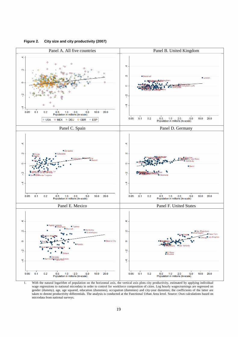
Figure 2 presents the level of city productivity premiums on the vertical axis and plots these against

the size of the city – as measured by its resident population. Panel A combines the five countries studied in

this paper while Panels B to F are disaggregated by country. For all countries studied, productivity is

higher in larger cities; an upward trend is identified in each of the country cases, though with varying

degrees of steepness. Countries differ also in the extent to which productivity varies across cities of similar

size, with city productivity in Germany, the United Kingdom and the United States being far more

homogenous than the productivity across cities in Spain or Mexico.

In the case of the United Kingdom, it is interesting, but perhaps unsurprising, to note that city

productivity premiums in London are larger even than those that would be expected given its size.

Furthermore, alongside human capital, proximity to London appears to account for much of the

performance of the positive outliers. Bracknell, Wokingham, Basingstoke, High Wycombe and Guilford –

all with high levels of tertiary education – are all within a 50km radius from London (with the exception of

Basingstoke, which is located 77km away). In contrast, there is no specific geographical pattern among the

negative outliers, but all have education levels below the UK average.10

9 . Combes, Duranton and Gobillon (2011) find the same range in their review of the literature.

10 . Walsall and Hastings are the two largest negative outliers. The former is an industrial town in West

Midlands with particularly low levels of tertiary education at 12%, and the latter a south-east town with

similarly low tertiary education levels at 15%. The average share of university graduates across UK cities

was 19% in 2007.

8

In Spain, city productivity premiums in Madrid are slightly below what would be expected given its

size, a result that is, in part, driven by particularly strong city productivity premiums in a number of mid-

sized cities. In Germany, the most noteworthy feature is probably the strong east-west divide, with city

productivity premiums in East German cities being, on the whole, significantly below the levels found in

West German cities of comparable size. In line with this finding, the city productivity premium in Berlin

lies in between the trends in East and West Germany. It is also noteworthy that a number of mid-sized

German cities have city productivity premiums at levels similar to Munich, Stuttgart and Frankfurt – the

most productive large agglomerations. This probably reflects a number of highly productive SME clusters

in the manufacturing sector that – often for historical reasons – are located in smaller agglomerations.

In Mexico, there is a clear north-south divide. Negative outliers are mostly agglomerations in the

south of the country, whereas positive outliers are generally located in the north, on or close to the US

border. In contrast, some of the negative outliers in the United States are located on or close to the Mexican

border. Also, other underperforming cities (including Chicago and Los Angeles) are relatively sprawled

cities with low employment densities and relatively fragmented labour markets.11

The descriptive country charts in Figure 3 illustrate the degree to which administrative fragmentation

is associated with productivity levels in cities. The degree of fragmentation of urban areas is measured by

the number of municipalities per 100,000 inhabitants.12

The charts show a tendency for more fragmented

cities to have lower levels of economic productivity. The effect varies across countries and is largest in

Mexico (Panel E).

For some time, the urban planning literature has highlighted the role of horizontal co-operation and

coordination among local governments as a substitute for administrative consolidation in enhancing urban

productivity (e.g. Blair, Staley and Zhang, 1996). This substitutability may shed some light on the strength

of the impact of fragmentation in Mexico. Mayors of Mexican cities are elected for a three year term and

are prohibited from running for immediate re-election. Furthermore, a large share of civil servants is

replaced after each election cycle. This discontinuity in personnel may render it difficult to establish lasting

co-operation across municipalities, potentially multiplying effects of fragmentation. In contrast, in the

other countries, many cities have reasonably well-functioning coordination bodies, which – to some degree

– may mitigate problems of fragmentation.

11 . In the case of Chicago, a relatively fragmented labour market, due to deficiencies in the public transport

system, might contribute to its underperformance (c.f. OECD, 2012b).

12 . Municipalities for Germany, Mexico, Spain; local authority districts for the United Kingdom, and counties

for the United States.

9

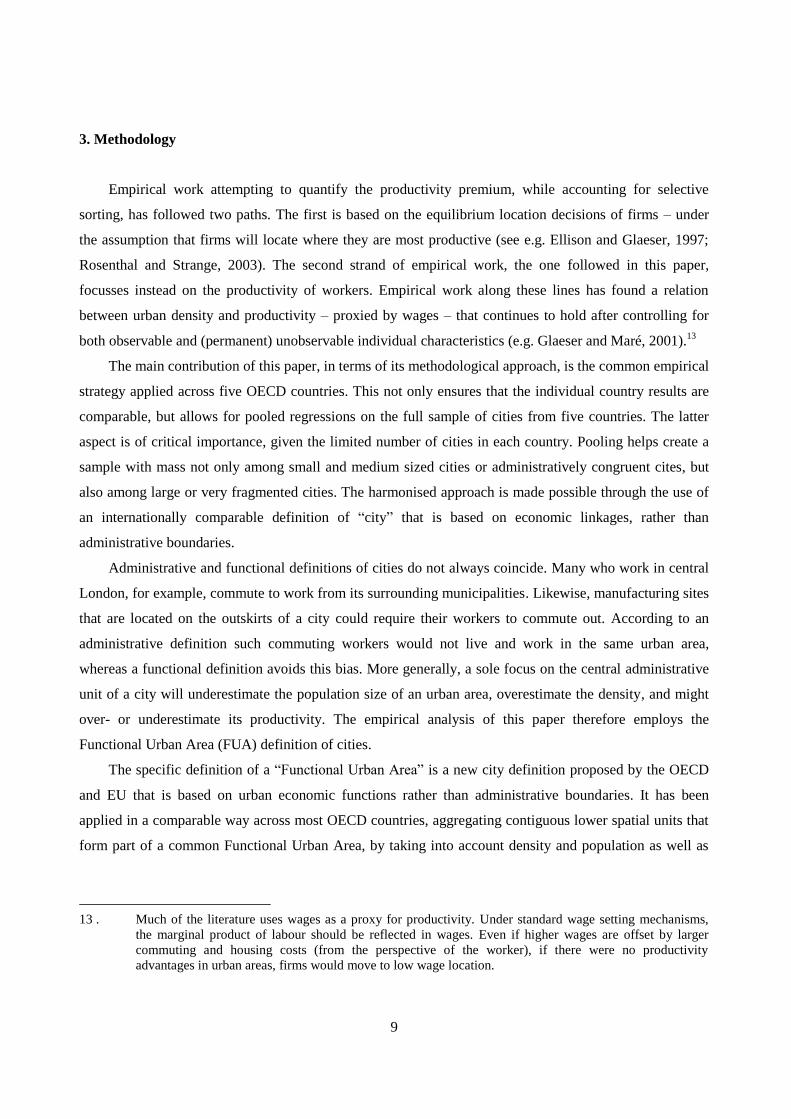
3. Methodology

Empirical work attempting to quantify the productivity premium, while accounting for selective

sorting, has followed two paths. The first is based on the equilibrium location decisions of firms – under

the assumption that firms will locate where they are most productive (see e.g. Ellison and Glaeser, 1997;

Rosenthal and Strange, 2003). The second strand of empirical work, the one followed in this paper,

focusses instead on the productivity of workers. Empirical work along these lines has found a relation

between urban density and productivity – proxied by wages – that continues to hold after controlling for

both observable and (permanent) unobservable individual characteristics (e.g. Glaeser and Maré, 2001).13

The main contribution of this paper, in terms of its methodological approach, is the common empirical

strategy applied across five OECD countries. This not only ensures that the individual country results are

comparable, but allows for pooled regressions on the full sample of cities from five countries. The latter

aspect is of critical importance, given the limited number of cities in each country. Pooling helps create a

sample with mass not only among small and medium sized cities or administratively congruent cites, but

also among large or very fragmented cities. The harmonised approach is made possible through the use of

an internationally comparable definition of “city” that is based on economic linkages, rather than

administrative boundaries.

Administrative and functional definitions of cities do not always coincide. Many who work in central

London, for example, commute to work from its surrounding municipalities. Likewise, manufacturing sites

that are located on the outskirts of a city could require their workers to commute out. According to an

administrative definition such commuting workers would not live and work in the same urban area,

whereas a functional definition avoids this bias. More generally, a sole focus on the central administrative

unit of a city will underestimate the population size of an urban area, overestimate the density, and might

over- or underestimate its productivity. The empirical analysis of this paper therefore employs the

Functional Urban Area (FUA) definition of cities.

The specific definition of a “Functional Urban Area” is a new city definition proposed by the OECD

and EU that is based on urban economic functions rather than administrative boundaries. It has been

applied in a comparable way across most OECD countries, aggregating contiguous lower spatial units that

form part of a common Functional Urban Area, by taking into account density and population as well as

13 . Much of the literature uses wages as a proxy for productivity. Under standard wage setting mechanisms,

the marginal product of labour should be reflected in wages. Even if higher wages are offset by larger

commuting and housing costs (from the perspective of the worker), if there were no productivity

advantages in urban areas, firms would move to low wage location.

10

commuting patterns (OECD, 2012a). The results are 1,148 largely self-contained urban labour markets

with at least 50,000 inhabitants across 28 OECD member states (OECD, 2012a).14

Specifically, municipalities or similarly small administrative units are used to build up the Functional

Urban Areas in a comparable way across countries. Units that include a majority of its population living in

high-density contiguous grids of 1,500 inhabitants per square kilometre (km2) are designated as “urban

centres”.15

Urban centres that have more than 15% of their population commuting from one to the other are

considered to belong to the same FUA. Less densely populated municipalities that have at least 15% of

their workforce commuting to an urban centre are included in the same FUA and form its commuting zone.

To address the concern of non-random sorting of skilled individuals, a two-step empirical approach is

applied separately to national microdata surveys for the five countries in the study (see Combes, Duranton

and Gobillon, 2011, for a theoretical discussion of this methodology).16

In the first step, the functional

OECD-EU definition of cities is matched with large scale administrative or survey-based microdata from

each of the five countries. The resulting data sets are then used to estimate productivity differentials – net

of individual skill differences and other individual level observables – across cities using an OLS

regression of the natural logarithm of wages on individual level characteristics and a set of fixed effects for

each city-year combination.17

𝑦𝑖𝑎𝑡 = 𝛽𝑋𝑖𝑎𝑡 + 𝛾𝑎𝑡𝑑𝑖𝑎𝑡 + 휀𝑖𝑎𝑡 (1)

𝑦𝑖𝑎𝑡 denotes the natural logarithm of wages for individual 𝑖 in city 𝑎 at time 𝑡, 𝑋 a vector of individual

characteristics, 𝑑 a vector of dummy variables that take the value 1 if the individual resides in the city 𝑎 at

time 𝑡, and 휀 denotes an error term. The coefficient vector of interest, 𝛾, captures the productivity

differential across cities, net of (observable) skill differences.

Since the primary concern in this study is to create comparable estimates for all five countries

(Germany, Mexico, Spain, United Kingdom, and United States), the specific controls that can be included

are limited to the controls available in all five data sets. Not all variables are available in all countries and

the different data sources include both panel data as well as repeated cross-sections. The common set of

14 . For the United States the local unit matched differs between small and medium-sized Functional Urban

Areas (with 50,000-500,000 inhabitants) and metropolitan areas with more than 500,000 inhabitants.

Therefore this study only considers only metropolitan areas for the United States.

15 . For Canada and the United States the threshold deviates and is set at 1,000 inhabitants per km2.

16 . See Combes, Duranton and Gobillon (2008) or Monastiriotis (2002) for earlier implementations of the

empirical methodology.

17 . This model follows the seminal work by Mincer (1974) and the large body of empirical literature that

followed it. The German data is right-censored, which introduces a bias in OLS estimation. However

comparing the results from a Tobit model, which accounts for censoring, and the OLS model shows that

the bias is negligible (see Ahrend and Lembcke, 2014).

11

controls selected includes age (and its square), education (dummies for degree categories), occupation

(dummies for occupational categories), gender (dummy) and an indicator for part-time work (dummy), in

addition to the city-year fixed effects.18

The city-year fixed effects obtained in the first step capture city productivity differentials, net of the

observable skill-relevant characteristics of the urban workforce for each of the five countries (𝑐). The

estimated productivity differentials (𝛾𝑐𝑎𝑡) are used as the dependent variable in the second step, in which

they are regressed on indicators for structural and organisational determinants of city productivity – both

time varying (𝑄𝑐𝑎𝑡) and non-time varying (𝑍𝑐𝑎). Additional country-year fixed effects 𝑑𝑐𝑡 control for time-

fixed differences across countries, national business cycles and country specific inflation (the first step

estimates nominal productivity differentials).

𝛾𝑐𝑎𝑡 = 𝛿𝑄𝑐𝑎𝑡 + 𝜇𝑍𝑐𝑎 + 𝜃𝑑𝑐𝑡 + 𝑢𝑐𝑎𝑡 (2)

The standard errors in the OLS estimation are clustered at the city level to allow for heteroscedasticity

and arbitrary autocorrelation over time (for each city) in the error term. In addition to the main

specification, which uses a balanced panel of all cities for the three years that are available for all five

countries (2005-2007), estimates are reported on a subsample that focuses on metropolitan areas – cities

with more than 500,000 inhabitants – only. This restriction is necessary as data on the presence of formal

co-operation arrangement across municipal boundaries (in the form of metropolitan governance bodies) are

only available for metropolitan areas. Furthermore, an alternative indicator for administrative

fragmentation, previously used in the literature, is used as a robustness check. A second robustness check

aims at assessing whether individual countries in the study are driving the results. Since the number of

metropolitan areas in each country is small, individual country regressions that evaluate the link between

governance structures and productivity are infeasible. Instead, a jackknife-style procedure is used, i.e. the

key results are re-estimated using a sample that leaves out one of the countries at a time.

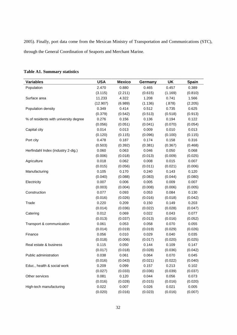
There is a range of city characteristics (𝑄𝑐𝑎𝑡 and 𝑍𝑐𝑎) considered in this study. The five countries’

samples are used to construct city-year indicators that capture city size, industrial structure and human

capital. The share of employees working in 1-digit industries, with manufacturing split into four categories

based on technology intensity, and the Herfindahl index of employment shares at the 2-digit industry level

are used to capture the industrial structure. The Herfindahl index is defined for each city as the sum of the

squared employment shares in each industry. The country samples are also used to estimate the population

18 . Panel data are available for three countries (Germany, Spain, and United Kingdom). The common

specification can therefore not account for individual specific unobserved skill differences in the first step.

Results for such specification are reported in separate individual country studies. See Ahrend and Lembcke

(forthcoming) for Germany, Georgiadis and Kaplanis (forthcoming) for the United Kingdom, and Diaz and

Kaplanis (forthcoming) for Spain. Kaplanis and Tello (forthcoming) report additional results for Mexico

that, however, do not allow for panel estimation.

12

in each FUA and year.19

Finally, the share of university degree holders among the 25-64 year old

workforce in the city is used as a measure for human capital. Further descriptions of the data used for each

country, as well as summary statistics, are provided in the Appendix.

The indicators constructed from the different country samples are then combined with data from the

OECD Metropolitan Database on administrative fragmentation (the number of local governments within a

city), the presence of a governance body (from Ahrend, Gamper and Schumann, 2014), a dummy variable

for the presence of a port in the city (based on data from Lloyd’s List “Ports”), and the surface area

covered by the city (own calculations from different administrative sources).20

The measure of

administrative fragmentation refers to an earlier time period (2001) than the estimated city-year

productivity differentials (2005-2007), which thus alleviates endogeneity concerns.

4. Empirical results

Putting numbers to the suggestive trends in the descriptive graphs of Section 2, country-by-country

regressions show productivity to be higher in larger cities across all five countries in this study (Table 1).

When city productivity differentials are regressed on city population, the estimated elasticities range from

0.016 (United Kingdom) to 0.063 (United States). That is, a US city with double the population of another

comparable US city is, on average, about 6.3% more productive.21

The main results from the pooled

regression, reported in Table 2, present equally strong evidence for sizeable agglomeration benefits. They

indicate that, a city with double the number of residents is associated with 3.8%higher productivity.

The source of agglomeration benefits can be further disentangled by a specification that uses both

population density and surface area of the city. The coefficient of (ln) population density gives the

elasticity of city productivity with respect to its size, holding constant the surface area covered by the city.

The coefficient on (ln) city surface area captures the impact of an expansion of city limits while population

density remains constant; that is, when population and area expand at the same rate. Finally, the difference

19 . Spain and Germany are exceptions. For Spain, internal OECD estimates for city population are used. For

Germany, only total employment can be observed; after the results from the last German census,

municipality level population data became unavailable. To estimate population in German FUAs the ratio

of employment to population for 2000 (OECD estimates) is used to rescale the observed employment

levels for all years.

20 . For the OECD Metropolitan database see: http://dotstat.oecd.org/Index.aspx?Datasetcode=CITIES and

http://www.oecd.org/gov/regional-policy/functionalurbanareasbycountry.htm. For port cities see

http://directories.lloydslist.com/ accessed 01.07.2013.

21 . Interpreting the elasticity multiplied by 100 as the percent increase in productivity associated with a

“doubling in city size” is commonly used in the literature to give an idea of the size of the impact. The

interpretation is not exact as the ln-approximation error is only negligible for small changes. The exact

marginal effect for a doubling in city size is the product of the estimated coefficient with ln(2)≈0.693.

13

between the area and the density coefficients gives the estimated impact of increasing the surface area

covered by a city while holding the total population constant (i.e. decreasing density with the given

population spreading out over a larger surface).

Interestingly, coefficients for population and area are similar (Table 2, second column), indicating that

both an increased population for a given surface area, and an increased spatial extent, while population

density remains constant, have similar productivity effects. As explained, the impact of an increase in the

spatial extent of a FUA, holding the population constant, is calculated as the difference between these two

elasticities. In this specification the difference is zero. This confirms that – for a given population –

agglomeration benefits do not increase with the surface area covered by a city. The introduction of

additional city characteristics as controls leads to estimated agglomeration elasticities ranging from 0.02 to

0.05, with highly statistically significant coefficients in all specifications (Table 2, remaining columns).

In addition to agglomeration benefits, the focus in this study is on horizontal governmental

fragmentation. An indicator for fragmentation is included in Table 2 from the third column onwards. It is

measured as the natural logarithm of the number of municipalities within a city.22

It is important to note

that the specification controls for city size, since size is already captured by the population density and area

indicators in the regression. The variable is also implicitly normalised for each country since the empirical

specification includes a full set of country-year fixed effects. The result of the inclusion of this variable is a

striking productivity penalty for more fragmented cities. The estimated coefficient (-0.032) is negative and

highly statistically significant. It indicates that between two cities of the same size, in the same country, if

one has twice the number of municipalities within its functional boundaries it is on average about 3.2%

less productive. The magnitude of this result remains largely unaffected when further controls are

introduced to the estimation.

The penalty is likely to be a lower bound for the impact of administrative fragmentation. Co-operation

and coordination across municipalities, for example in the form of governance bodies, is common in

OECD countries and can alleviate, to some extent, the problems associated with fragmentation. If this is

the case, not explicitly controlling for coordination bodies will result in underestimates of the true extent of

the fragmentation penalty (i.e. the estimated coefficient is too small in absolute value).

Ahrend, Gamper and Schumann (2014) collect information on governance bodies for OECD

metropolitan areas, i.e. Functional Urban Areas with at least 500,000 inhabitants, a subset of the cities

considered in this study. Accounting explicitly for governance bodies therefore limits the analysis to 140

metropolitan areas. While this decrease in the size of the available sample reduces the available degrees of

22 . Local authority districts for the United Kingdom and counties for the United States.

14

freedom and therefore the precision of the estimates, especially when the full set of controls is considered,

it can nonetheless shed some light on the true impact of fragmentation.

To ensure that estimates on the selected sample are comparable, Table 3 replicates the key results

from Table 2, for metropolitan areas only. The estimates are similar compared to the specification that

includes the full sample of cities. The impact of administrative fragmentation is the same, but point

estimates for agglomeration benefits are slightly higher. This difference is however not statistically

significant. Columns III, V, and VII introduce the impact of horizontal fragmentation in metropolitan areas

with and without the mediating presence of a metropolitan governance body. The estimated impact of

horizontal fragmentation becomes even more severe when the presence of governance bodies is taken into

account. Without a governance body the negative impact on productivity is about 6%. The fragmentation

penalty is halved if the city has a governance body. With a governance body, a doubling of the number of

municipalities is associated with just 2.5-3% lower productivity.23

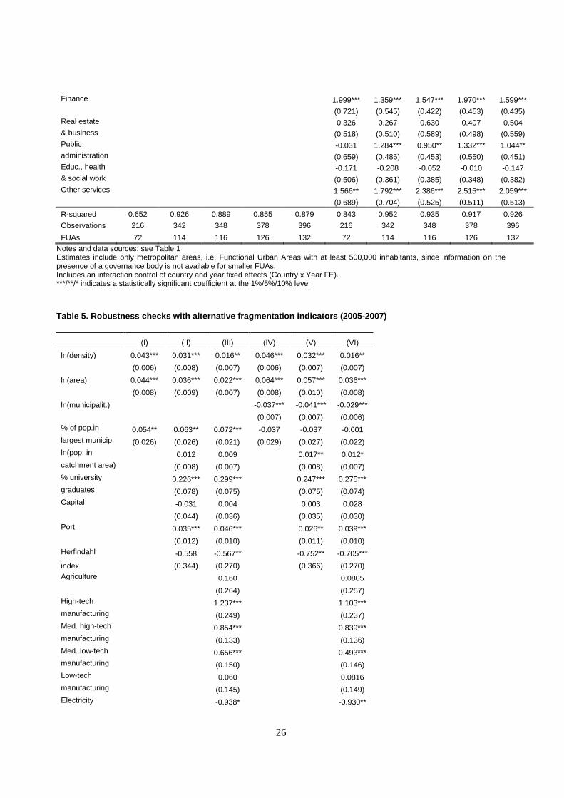
Given the small number of metropolitan areas in each country, it is not possible to consider the impact

of fragmentation and governance bodies in each separately. However, it is possible to use a jackknife

approach and re-estimate the models excluding one country at a time, which can reveal whether the results

are driven by a single country. Table 4 presents the results with each column excluding the metropolitan

areas from the indicated country. Without controlling for industry shares the results are qualitatively the

same as the main results in Table 3. The weakest impact of administrative fragmentation is found when

Mexico is excluded from the model, but even in this specification the productivity penalty is 3.2%. For the

remaining subsamples the estimates range from 5-8% with governance bodies alleviating 40-60% of the

impact. For completeness, the table also reports results that include industry shares, results that suffer from

severe identification problems as the number of degrees of freedom in these models becomes very small.24

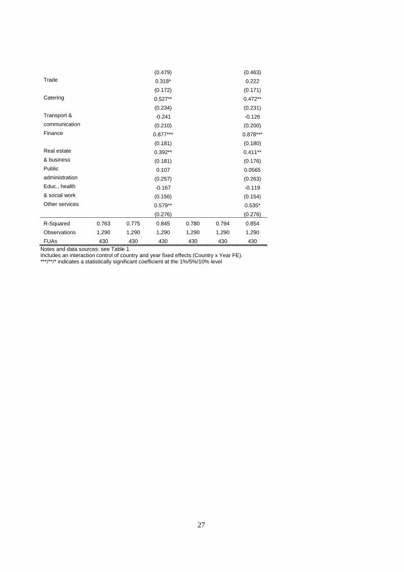
Arguing that coordination is simplified if residents are heavily concentrated in a single administrative

unit, Cheshire and Magrini (2009) proxy for the degree of fragmentation in urban regions using the

proportion of residents living in the largest municipality. Table 5 considers this alternative measure of

fragmentation. The results in the first three columns show that concentration of a city’s inhabitants does

indeed appear to ease fragmentation penalties. A 10 percentage point decrease in the share of the

population residing in the core municipality is estimated to reduce productivity, on average, by 0.5-0.7%.

23 . The coefficient on the interaction term indicates the difference in the impact of fragmentation for cities that

do have a governance body compared to cities that do not have a governance body. E.g. the marginal effect

of an increase in (ln) fragmentation in column (III) of Table 3 is: -0.057 + 0.031 x gov.body

24 . Standard errors are clustered at the metropolitan area level, which makes the number of metropolitan areas

and not the number of observations the base degree of freedom.

15

One might take this result to also indicate that the estimated penalty from administrative fragmentation is

not truly related to the cities’ governance, but captures some unfavourable effects of urban structure.25

However, when both indicators, concentration and administrative fragmentation, are combined in the

same specification – columns (IV) through (VI) – horizontal fragmentation measured by the (natural

logarithm) of the number of municipalities is very robust and in line with the main estimates, but

concentration of residents becomes insignificant. Dominance of a single municipality, in terms of the share

of residents, cannot solve the coordination problems raised by fragmentation and it is the presence of

administrative boundaries, rather than urban structure that turns out to be the more relevant measure. To

capture the urban structure, we have experimented by using the Herfindahl Index of the population across

municipalities within the city, which should account to some extent for the density distribution within the

city. The Herfindahl Index behaves qualitatively in a similar pattern with the population share in the largest

municipality and does not change the reported results. Therefore, while urban structure can certainly have

an impact on local conditions, our results suggest that administrative fragmentation still plays a key role

when it comes to urban productivity premia.

Going back to Table 2 and the remaining indicators, aggregate human capital, measured by the share

of university graduates in the city, increases productivity. A 10 percentage point increase in the share of

university graduates is associated with a 3% increase in productivity. It is important to note that this result

does not indicate the direct impact of human capital on productivity, but only the externality associated

with working in a city with many university graduates. And, while port cities exhibit higher productivity –

on average port cities are 2-4% more productive than comparable cities without a port – there appears to be

no evidence that capitals differ systematically from other cities.

Industrial specialisation, measured by the normalised Herfindahl Index of employment shares at the 2-

digit industry level, has a negative and weakly significant impact. This suggests that a diversified industrial

structure has a positive impact on productivity. However, variation in estimates across specifications

suggests that this finding is not overly robust. Moreover, clear evidence can be found that cities with a high

share of employees in specific industries exhibit higher productivity. The base category in the regressions

is the share of employees in construction, such that when an increase in an industry share is considered, the

share of employees in construction is reduced by the same amount. The results (column IX in Table 2)

indicate that a 1 percentage point increase in the share of high-tech manufacturing workers (and a

concomitant one percentage point decrease in the share of construction workers) is, on average, associated

with a 1.2% increase in productivity in the city. This productivity premium gradually reduces with the

technological intensity of the manufacturing industry: it is 0.8% and 0.6% for medium-high-tech and

25 . The authors would like to thank the anonymous referee who voiced this concern.

16

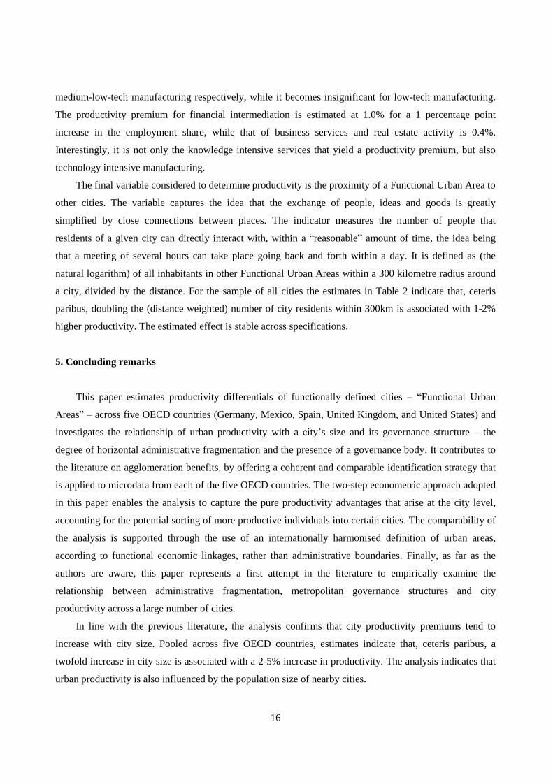
medium-low-tech manufacturing respectively, while it becomes insignificant for low-tech manufacturing.

The productivity premium for financial intermediation is estimated at 1.0% for a 1 percentage point

increase in the employment share, while that of business services and real estate activity is 0.4%.

Interestingly, it is not only the knowledge intensive services that yield a productivity premium, but also

technology intensive manufacturing.

The final variable considered to determine productivity is the proximity of a Functional Urban Area to

other cities. The variable captures the idea that the exchange of people, ideas and goods is greatly

simplified by close connections between places. The indicator measures the number of people that

residents of a given city can directly interact with, within a “reasonable” amount of time, the idea being

that a meeting of several hours can take place going back and forth within a day. It is defined as (the

natural logarithm) of all inhabitants in other Functional Urban Areas within a 300 kilometre radius around

a city, divided by the distance. For the sample of all cities the estimates in Table 2 indicate that, ceteris

paribus, doubling the (distance weighted) number of city residents within 300km is associated with 1-2%

higher productivity. The estimated effect is stable across specifications.

5. Concluding remarks

This paper estimates productivity differentials of functionally defined cities – “Functional Urban

Areas” – across five OECD countries (Germany, Mexico, Spain, United Kingdom, and United States) and

investigates the relationship of urban productivity with a city’s size and its governance structure – the

degree of horizontal administrative fragmentation and the presence of a governance body. It contributes to

the literature on agglomeration benefits, by offering a coherent and comparable identification strategy that

is applied to microdata from each of the five OECD countries. The two-step econometric approach adopted

in this paper enables the analysis to capture the pure productivity advantages that arise at the city level,

accounting for the potential sorting of more productive individuals into certain cities. The comparability of

the analysis is supported through the use of an internationally harmonised definition of urban areas,

according to functional economic linkages, rather than administrative boundaries. Finally, as far as the

authors are aware, this paper represents a first attempt in the literature to empirically examine the

relationship between administrative fragmentation, metropolitan governance structures and city

productivity across a large number of cities.

In line with the previous literature, the analysis confirms that city productivity premiums tend to

increase with city size. Pooled across five OECD countries, estimates indicate that, ceteris paribus, a

twofold increase in city size is associated with a 2-5% increase in productivity. The analysis indicates that

urban productivity is also influenced by the population size of nearby cities.

17

Crucially, this paper identifies a significant role for horizontal administrative fragmentation of a city’s

governance structure in determining the magnitude of city productivity premiums. Specifically, for two

cities of similar size and population composition in terms of observable characteristics, but with one city

having twice the number of municipalities, the estimates indicate that productivity in the more fragmented

city is between 3 and 4% lower. The estimate is likely a lower bound, as alleviating mechanisms are likely

to be present. This study finds that if the presence of a metropolitan governance body is taken into account,

the fragmentation penalty lies around 6%, with governance bodies alleviating the penalty to about half its

size.

While the presence of a governance body mitigates the negative effect of fragmentation, little is

known about the underlying transmission mechanisms from administrative fragmentation, via governance

arrangements to stymied productivity. Important policy areas that are likely to create inefficient outcomes

at the metropolitan level are land-use and transport polices, which can greatly benefit from adequate

metropolitan coordination. Descriptive evidence suggests that the presence of governance bodies is

associated with less sprawling development, and that transport authorities at the metropolitan level are

linked with better quality in public transport provision (Ahrend, Gamper and Schumann, 2014). But the

influence of administrative fragmentation may stem from a variety of associated factors and warrants

further investigation. This paper constitutes a first attempt to establish a link between governance

arrangements and economic outcomes; a full examination of the causes of lower productivity in more

administratively fragmented urban areas will require more detailed information on urban governance

structures.

18

Figures and tables

Figure 1. City size and labour productivity (2010)

Notes: Labour Productivity is measured as GDP (Millions of US$ constant PPP, constant prices, reference year is 2005) divided by the total number of employees in a Functional Urban Area. Data refer to 2010 or the closest available year.

Data source: OECD Metropolitan Explorer.

19

Figure 2. City size and city productivity (2007)

Panel A. All five countries Panel B. United Kingdom

Panel C. Spain Panel D. Germany

Panel E. Mexico Panel F. United States

1. With the natural logarithm of population on the horizontal axis, the vertical axis plots city productivity, estimated by applying individual

wage regressions to national microdata in order to control for workforce composition of cities. Log hourly wages/earnings are regressed on

gender (dummy), age, age squared, education (dummies), occupation (dummies) and city-year dummies; the coefficients of the latter are

taken to denote productivity differentials. The analysis is conducted at the Functional Urban Area level. Source: Own calculations based on microdata from national surveys.

20

Figure 3. Horizontal administrative fragmentation and city productivity

Panel A. All five countries Panel B. United Kingdom

Panel C. Spain Panel D. Germany

Panel E. Mexico Panel F. United States

1. See note of Figure 1. Fragmentation is the number of municipalities per 100,000 inhabitants.

21

Table 1. Regressions from individual country regressions

UK Spain Germany US Mexico UK Spain Germany US Mexico

ln(population) 0.016* 0.034*** 0.037*** 0.063*** 0.042**

(0.009) (0.012) (0.010) (0.008) (0.020)

ln(pop.density)

0.009 0.046*** 0.068*** 0.066*** 0.022

(0.009) (0.011) (0.010) (0.009) (0.019)

ln(area)

0.019* 0.032** 0.020** 0.058*** 0.083***

(0.01) (0.013) (0.009) (0.010) (0.021)

R-squared 0.666 0.294 0.191 0.914 0.483 0.649 0.314 0.328 0.915 0.569

Observations 808 532 981 345 825 808 532 981 345 825

FUAs 101 76 109 69 75 101 76 109 69 75

Notes: Table reports OLS regressions with estimated Functional Urban Area (FUA) productivity as dependent variable. FUA productivity is estimated by applying individual wage regressions to national microdata in order to control for workforce composition of cities. Log hourly wages/earnings are regressed on a gender (dummy), age, age squared, education (dummies), occupation (dummies) and city-year dummies; the coefficients of the latter are taken to denote productivity differentials. (see text for details). Variable definitions in section 4. Standard errors are clustered at the Functional Urban Area level, all specifications include time fixed effects. Data sources: UK: ASHE/LFS; Spain: MCVL; Germany: IAB; US: IPUMS; Mexico: ENE/ENOE ***/**/* indicates a statistically significant coefficient at the 1%/5%/10% level Sample years are: 2003-2010 (UK); 2005-2011 (Spain); 1999-2007 (Germany); 1990, 2000, 2005-2007 (US); 2000-2010 (Mexico)

22

Table 2. Pooled regressions: common years (2005-2007)

(I) (II) (III) (IV) (V) (VI) (VII) (VIII) (IX) (X)

ln(population) 0.038***

(0.005)

ln(density)

0.038*** 0.048*** 0.045*** 0.042*** 0.043*** 0.037*** 0.034*** 0.018*** 0.016**

(0.006) (0.006) (0.006) (0.006) (0.006) (0.007) (0.007) (0.007) (0.007)

ln(area)

0.038*** 0.064*** 0.070*** 0.066*** 0.066*** 0.062*** 0.058*** 0.039*** 0.036***

(0.006) (0.008) (0.009) (0.009) (0.009) (0.009) (0.010) (0.008) (0.008)

ln(municipalit.)

-0.032*** -0.035*** -0.037*** -0.037*** -0.036*** -0.036*** -0.029*** -0.029***

(0.006) (0.006) (0.006) (0.006) (0.006) (0.006) (0.005) (0.005)

ln(pop. in 0.017** 0.015* 0.015* 0.018** 0.017** 0.013* 0.012*

catchment area) (0.008) (0.008) (0.008) (0.008) (0.008) (0.007) (0.007)

% university

0.273*** 0.275*** 0.283*** 0.258*** 0.287*** 0.275***

graduates

(0.077) (0.077) (0.077) (0.075) (0.076) (0.073)

Capital

-0.017 -0.011 -0.000 0.019 0.028

(0.042) (0.037) (0.038) (0.030) (0.030)

Port

0.027** 0.027** 0.038*** 0.039***

(0.011) (0.011) (0.010) (0.010)

Herfindahl

-0.698* -0.704***

index

(0.358) (0.266)

Agriculture

0.085 0.0808

(0.253) (0.257)

High-tech 1.176*** 1.104***

manufacturing (0.227) (0.234)

Med. high-tech 0.824*** 0.840***

manufacturing (0.140) (0.135)

Med. low-tech 0.591*** 0.494***

manufacturing (0.146) (0.146)

Low-tech

0.069 0.082

manufacturing

(0.161) (0.149)

Electricity

-0.812* -0.931**

(0.454) (0.463)

Trade

0.229 0.223

(0.174) (0.171)

Catering

0.381 0.472**

(0.259) (0.230)

Transport &

0.002 -0.126

communication

(0.193) (0.200)

Finance

0.955*** 0.878***

(0.176) (0.181)

Real estate

0.449** 0.410**

& business

(0.183) (0.176)

Public

0.079 0.057

administration

(0.260) (0.261)

Educ., health

-0.100 -0.120

& social work

(0.157) (0.154)

Other services

0.561** 0.535*

(0.276) (0.275)

R-Squared 0.760 0.760 0.779 0.783 0.788 0.788 0.791 0.794 0.852 0.854

23

Observations 1,290 1,290 1,290 1,290 1,290 1,290 1,290 1,290 1,290 1,290

FUAs 430 430 430 430 430 430 430 430 430 430

Notes and data sources: see Table 1 Includes an interaction control of country and year fixed effects (Country x Year FE). ***/**/* indicates a statistically significant coefficient at the 1%/5%/10% level

24

Table 3. Pooled regressions on governance indicators (2005-2007)

(I) (II) (III) (IV) (V) (VI) (VII)

ln(density) 0.049*** 0.064*** 0.065*** 0.049*** 0.047*** 0.035*** 0.035***

(0.011) (0.012) (0.012) (0.012) (0.012) (0.010) (0.011)

ln(area) 0.057*** 0.082*** 0.085*** 0.086*** 0.087*** 0.069*** 0.070***

(0.010) (0.012) (0.012) (0.014) (0.013) (0.014) (0.014)

ln(municipalit.) -0.032*** -0.057*** -0.035*** -0.066*** -0.029*** -0.033***

(0.010) (0.016) (0.008) (0.017) (0.007) (0.013)

ln(municipalit.) 0.031** 0.036** 0.006

× govern. body (0.014) (0.015) (0.011)

Governance -0.079** -0.092** -0.024

Body (0.034) (0.038) (0.027)

ln(pop. in 0.021** 0.022** 0.013 0.013

catchment area) (0.010) (0.010) (0.008) (0.008)

% university 0.426*** 0.478*** 0.378** 0.390**

graduates (0.150) (0.138) (0.155) (0.152)

Capital -0.051 -0.025 -0.046* -0.045

(0.039) (0.040) (0.027) (0.030)

Port 0.026* 0.025* 0.030*** 0.031***

(0.014) (0.013) (0.010) (0.010)

Herfindahl -1.013 -1.136 0.492 0.349

index (1.332) (1.328) (0.846) (0.858)

Agriculture 0.378 0.429

(0.556) (0.547)

High-tech 1.073** 0.998**

manufacturing (0.436) (0.450)

Med. high-tech 1.077*** 1.052***

manufacturing (0.335) (0.344)

Med. low-tech 2.031*** 2.003***

manufacturing (0.544) (0.544)

Low-tech 1.054*** 1.076***

manufacturing (0.356) (0.352)

Electricity -0.488 -0.412

(1.408) (1.433)

Trade 0.687 0.704

(0.475) (0.480)

Catering 0.184 0.130

(0.780) (0.729)

Transport & -0.029 -0.0766

communication (0.574) (0.583)

Finance 1.717*** 1.668***

(0.421) (0.420)

Real estate 0.352 0.420

& business (0.493) (0.487)

Public 1.028** 1.023**

administration (0.466) (0.445)

Educ., health -0.134 -0.113

& social work (0.351) (0.341)

25

Other services 2.291*** 2.265***

(0.478) (0.491)

R-Squared 0.829 0.847 0.855 0.869 0.880 0.928 0.929

Observations 420 420 420 420 420 420 420

FUAs 140 140 140 140 140 140 140

Notes and data sources: see Table 1 Estimates include only metropolitan areas, i.e. Functional Urban Areas with at least 500,000 inhabitants, since information on the presence of a governance body is not available for smaller FUAs. Includes an interaction control of country and year fixed effects (Country x Year FE). ***/**/* indicates a statistically significant coefficient at the 1%/5%/10% level

Table 4. Pooled regressions excluding one (2005-2007)

Pooled estimates for USA, MEX, DEU, GBR & ESP, except:

USA MEX DEU GBR ESP USA MEX DEU GBR ESP

ln(pop.density) 0.068*** 0.037*** 0.048*** 0.048*** 0.055*** 0.024 0.039*** 0.031*** 0.036*** 0.039***

(0.028) (0.01) (0.012) (0.012) (0.011) (0.021) (0.010) (0.011) (0.011) (0.011)

ln(area) 0.140*** 0.059*** 0.092*** 0.092*** 0.088*** 0.068*** 0.052*** 0.066*** 0.072*** 0.069***

(0.026) (0.011) (0.014) (0.013) (0.013) (0.021) (0.012) (0.014) (0.014) (0.014)

ln(municipalit.) -0.075*** -0.032* -0.052*** -0.066*** -0.080*** -0.022* -0.018* -0.018 -0.032*** -0.044***

(0.022) (0.020) (0.021) (0.019) (0.016) (0.016) (0.013) (0.015) (0.013) (0.013)

ln(municipalit.) 0.027* 0.031** 0.024 0.037** 0.049*** -0.013 0.012 -0.007 0.003 0.014

× gov. body (0.020) (0.016) (0.019) (0.016) (0.015) (0.015) (0.011) (0.013) (0.011) (0.011)

Governance -0.054 -0.070** -0.084** -0.092*** -0.111*** 0.038 -0.027 -0.018 -0.017 -0.041*

body (0.055) (0.042) (0.041) (0.039) (0.036) (0.041) (0.026) (0.028) (0.030) (0.027)

ln(pop. in 0.029** 0.025** 0.022** 0.024*** 0.015** 0.016* 0.017** 0.011* 0.012* 0.009

catchm. area) (0.015) (0.012) (0.010) (0.01) (0.009) (0.011) (0.008) (0.008) (0.008) (0.008)

% university -0.020 0.489*** 0.593*** 0.532*** 0.459*** 0.108 0.396*** 0.418*** 0.427*** 0.319**

graduates (0.274) (0.138) (0.143) (0.165) (0.151) (0.320) (0.143) (0.164) (0.162) (0.164)

Capital -0.077 -0.021 -0.046 -0.044 -0.010 -0.024 -0.042* -0.062** -0.060** -0.029

(0.063) (0.035) (0.041) (0.047) (0.040) (0.051) (0.027) (0.031) (0.034) (0.032)

Port 0.001 0.024*** 0.027** 0.022* 0.028** 0.019 0.025*** 0.035*** 0.032*** 0.034***

(0.025) (0.009) (0.016) (0.015) (0.013) (0.017) (0.009) (0.011) (0.010) (0.009)

Herfindahl 0.330 0.028 0.440 0.449 0.344

index (1.159) (1.600) (0.976) (0.958) (0.905)

Agriculture -0.185 1.130* 0.528 0.566 0.341

(0.520) (0.700) (0.582) (0.561) (0.548)

High-tech -0.008 0.996 -2.132* -0.085 -0.389

manufacturing (2.265) (1.591) (1.469) (1.675) (1.466)

Med. high-tech 1.832*** 0.668* 0.914** 1.183*** 0.974**

manufacturing (0.596) (0.460) (0.461) (0.483) (0.462)

Med. low-tech 0.753* 0.903** 1.081*** 1.200*** 0.891***

manufacturing (0.487) (0.440) (0.340) (0.364) (0.348)

Low-tech 1.698*** 1.339*** 2.007*** 2.261*** 1.833***

manufacturing (0.689) (0.552) (0.661) (0.587) (0.573)

Electricity 0.255 1.289** 1.119*** 1.245*** 1.047***

(0.543) (0.602) (0.362) (0.366) (0.370)

Trade 1.351*** 0.459 0.581 0.886** 0.571

(0.554) (0.516) (0.529) (0.500) (0.479)

Catering -0.836 1.046* 0.175 0.385 -0.015

(0.848) (0.813) (0.751) (0.793) (0.693)

Transport & -0.759 -0.035 0.086 0.114 -0.185

communic. (0.860) (0.579) (0.635) (0.616) (0.601)

26

Finance 1.999*** 1.359*** 1.547*** 1.970*** 1.599***

(0.721) (0.545) (0.422) (0.453) (0.435)

Real estate 0.326 0.267 0.630 0.407 0.504

& business (0.518) (0.510) (0.589) (0.498) (0.559)

Public -0.031 1.284*** 0.950** 1.332*** 1.044**

administration (0.659) (0.486) (0.453) (0.550) (0.451)

Educ., health -0.171 -0.208 -0.052 -0.010 -0.147

& social work (0.506) (0.361) (0.385) (0.348) (0.382)

Other services 1.566** 1.792*** 2.386*** 2.515*** 2.059***

(0.689) (0.704) (0.525) (0.511) (0.513)

R-squared 0.652 0.926 0.889 0.855 0.879 0.843 0.952 0.935 0.917 0.926

Observations 216 342 348 378 396 216 342 348 378 396

FUAs 72 114 116 126 132 72 114 116 126 132

Notes and data sources: see Table 1 Estimates include only metropolitan areas, i.e. Functional Urban Areas with at least 500,000 inhabitants, since information on the presence of a governance body is not available for smaller FUAs. Includes an interaction control of country and year fixed effects (Country x Year FE). ***/**/* indicates a statistically significant coefficient at the 1%/5%/10% level

Table 5. Robustness checks with alternative fragmentation indicators (2005-2007)

(I) (II) (III) (IV) (V) (VI)

ln(density) 0.043*** 0.031*** 0.016** 0.046*** 0.032*** 0.016**

(0.006) (0.008) (0.007) (0.006) (0.007) (0.007)

ln(area) 0.044*** 0.036*** 0.022*** 0.064*** 0.057*** 0.036***

(0.008) (0.009) (0.007) (0.008) (0.010) (0.008)

ln(municipalit.) -0.037*** -0.041*** -0.029***

(0.007) (0.007) (0.006)

% of pop.in 0.054** 0.063** 0.072*** -0.037 -0.037 -0.001

largest municip. (0.026) (0.026) (0.021) (0.029) (0.027) (0.022)

ln(pop. in 0.012 0.009 0.017** 0.012*

catchment area) (0.008) (0.007) (0.008) (0.007)

% university 0.226*** 0.299*** 0.247*** 0.275***

graduates (0.078) (0.075) (0.075) (0.074)

Capital -0.031 0.004 0.003 0.028

(0.044) (0.036) (0.035) (0.030)

Port 0.035*** 0.046*** 0.026** 0.039***

(0.012) (0.010) (0.011) (0.010)

Herfindahl -0.558 -0.567** -0.752** -0.705***

index (0.344) (0.270) (0.366) (0.270)

Agriculture 0.160 0.0805

(0.264) (0.257)

High-tech 1.237*** 1.103***

manufacturing (0.249) (0.237)

Med. high-tech 0.854*** 0.839***

manufacturing (0.133) (0.136)

Med. low-tech 0.656*** 0.493***

manufacturing (0.150) (0.146)

Low-tech 0.060 0.0816

manufacturing (0.145) (0.149)

Electricity -0.938* -0.930**

27

(0.479) (0.463)

Trade 0.318* 0.222

(0.172) (0.171)

Catering 0.527** 0.472**

(0.234) (0.231)

Transport & -0.241 -0.126

communication (0.210) (0.200)

Finance 0.877*** 0.878***

(0.181) (0.180)

Real estate 0.392** 0.411**

& business (0.181) (0.176)

Public 0.107 0.0565

administration (0.257) (0.263)

Educ., health -0.167 -0.119

& social work (0.156) (0.154)

Other services 0.579** 0.535*

(0.276) (0.276)

R-Squared 0.763 0.775 0.845 0.780 0.794 0.854

Observations 1,290 1,290 1,290 1,290 1,290 1,290

FUAs 430 430 430 430 430 430

Notes and data sources: see Table 1 Includes an interaction control of country and year fixed effects (Country x Year FE). ***/**/* indicates a statistically significant coefficient at the 1%/5%/10% level

28

Appendix A. Data description and summary statistics

United Kingdom

The estimation of the first-stage is based on data from the UK Annual Survey of Hours and Earnings

(ASHE) for 2003-2010. ASHE is the largest survey on labour market statistics with approximately 160,000

employees a year. It is a random sample of around 1% of the National Insurance pool, as it tracks

employees whose national insurance ends with a specific pair of digits. The information is collected by

questionnaires sent to employers in April each year, with questions on wages, job and individual workers

characteristics. It is an unbalanced panel as individuals can be followed over time, but would drop from the

survey if they become unemployed or move to self-employment. The sample is restricted to main jobs

only.

ASHE provides detailed information on individual earnings and hours worked and for our analysis we

use gross hourly earnings as our wage measure. Additional information on individual characteristics

includes occupation, industry, whether the job is in the private or public sector, the worker’s age and

gender. Information on education is not available via ASHE and thus we have to impute education using

the UK Quarterly Labour Force Survey for 2003-2010. Specifically, an individual’s years of schooling in

ASHE are simulated using estimates of the coefficients of the Best Linear Predictor of education from the

Labour Force survey over the same period.26

Quarterly Labour Force Survey (QLFS) is also used to

construct most of the city controls of the second stage, like population, the share of university graduates,

Herfindahl Index (2-digit SIC2003) and the various industrial shares. A more detailed description of the

data used is offered in Georgiadis and Kaplanis (2014).

26 . In particular, education was simulated using coefficients' estimates of regressions of education on year of

birth and year of birth squared separately by two-digit occupation in the Quarterly LFS (2003-2010) and

information on year of birth and two-digit occupation code in ASHE. Other studies based in ASHE use

occupation controls as proxies for education arguing that the former is a fairly good proxy for the latter

(Kaplanis, 2010; Gibbons, Overman and Pelkonen, 2010).

29

Spain

For the empirical analysis, the Muestra Continua de Vidas Laborales, MCVL, (Continuous sample of

working histories), an administrative data set provided by the Social Security Administration is used. The

recently released MCVL contains information of individuals who had an active record with the Social

Security system at any time during the years 2005-2011. Each year the sample is a 4% non-stratified

random draw from a reference population that includes employed workers (wage earners and self-

employed), unemployment benefits recipients and pension earners. It consists of nearly 1.1 million

individuals per year. The MCVL tries to reconstruct the employment and contribution history of the

selected individuals. The information available on labour histories dates back to 1967 while earnings

records are tracked since 1980.

Individuals that are registered in the Social Security as wage earners between 2006 and 2011 are

selected and their working histories are used to construct most of the individual variables of the first stage.

Since 2006, the MCVL can be matched with the tax records, which contains the summary for each fiscal

year of all the withholdings and prepayments of personal income tax on earned income, economic

activities, prizes and income imputations. Since, the aim is to investigate issues related to wages, this data

is suitable as this category of income is well represented by the reliability and the general scope of the tax

data for earned income. These tax records allow the construction of an annual panel covering the period

2005-2011, with very precise information about individual earnings. Therefore all individual wages for all

workers in the MCVL for that period are accounted for. In order to have the maximum number of

observation the tax records are merged for all the available years, i.e. 2005-2011. The analysis is restricted

to wage earners, self-employed are left out of the sample.

The OECD defines 76 FUAs in Spain, which represents about 62% of the Spanish population. In the

MCVL, only municipalities with more than 40,000 inhabitants can be identified. For a detailed description

of the necessary adjustments in order to construct FUAs well as further information on the variables used

in the regressions, the reader should refer to the relevant OECD working paper (Diaz and Kaplanis, 2014).

30

Germany

For the German individual level regressions the Employment Panel of the German Federal

Employment Agency (BA) hosted by the Research Data Centre (FDZ) at the Institute for Employment

Research (IAB) is used.27

The data contains a 2% sample of all registered employees who are subject to

social security contributions on the reference date. The sample is a panel data set that covers the years from

1998 to 2007 and the on-site version of the data set contains information on the municipality (Gemeinde)

of residence.28

The data does not contain information on hours worked (other than part-time status). It is therefore

necessary to estimate earnings- rather than wage differentials across FUAs. As controls gender, age (and its

square), educational attainment, occupational standing (apprentice, white or blue collar, master craftsmen,

etc.: 7 categories), and occupation (3-digit) are added.

United States

For the United States of America the sample combines the U.S. Census from 1990 and 2000 with the

American Community Survey for the years 2005 to 2007. The data are provided as a scientific use-file by

the IPUMS project.29

The available information on county of residence is used to link the IPUMS data with

the OECD (2012a) definition of Functional Urban Areas. Since not all counties are identified in the

scientific use-file, the metropolitan statistical area/s (MSAs) that coincide with a FUA is identified and

observations from those MSAs are added. The resulting IPUMS based estimates for FUA size are close to

the corresponding OECD calculations.

To estimate the wage equations hourly wages are constructed as the sum of all earnings from wages in

the last year divided by the product of the number of hours usually worked per week in the previous year

and the number of weeks worked. The estimates include controls for part-time status (using the Bureau of

27 . See Schmucker and Seth (2009) for a detailed description of the data.

28 . The sample changes slightly in 1999. The study is therefore limited to the years 1999-2007.

29. Ruggles et al. (2010)

31

Labor Statistics definition of usually working less than 35 hours per week), gender, educational attainment,

age and its square, and occupation (3-digit codes). Sampling weights are used in all calculations.

Mexico

The data refer to 2000-2010 and come from the Labour Force Surveys (National Occupation and

Employment Survey, ENOE and the National Employment Survey, ENE), carried out by the National

Institute of Statistics and Geography of Mexico (INEGI). Data from 2000 to 2004 are derived from the

National Employment Survey (ENE) and from 2005 to 2010 data refer to the National Occupation and

Employment Survey (ENOE). Both are household surveys, whose selection units are dwellings selected by

sample techniques.

The Mexican labour force surveys (ENE and ENOE) are representative of urban and rural areas, as

well for each of the 32 Mexican States, include a quarterly rotating panel of survey respondents, and is a

rotating panel (rotation scheme of 20%, i.e., workers are observed at most five times over a five-quarter

period).

The data provide information on both economically active (labour force) and non-economically active

population and is referred to persons aged 15 years old onwards. The surveys cover social and

demographic information and provide details about job characteristics, incomes, work duration,

demographics and education. Schooling was aggregate in five categories: no schooling or incomplete

primary; complete primary; lower secondary; upper secondary and higher or tertiary. The data contain a

monthly earnings variable from which we calculate logarithmic hourly wages as the ratio of monthly

earnings to 4.3 times the hours worked weekly. For individuals who report their wages as a multiple of the

minimum wage, we assign as their wage the mean of the interval.

Additional city controls that are not from ENE or ENOE, have also been used. For city population we

use information from the Census for the years 2000, 2005 and 2010 and interpolate the intermediate years.

(Source: INEGI, General Census of Population and Housing, 2000, 2005 and 2010). For the land area, the

data come from the Mexican Statistical Office, INEGI (Cartography of land use and vegetation 2002 and

32

2005). Finally, port data come from the Mexican Ministry of Transportation and Communications (STC),

through the General Coordination of Seaports and Merchant Marine.

Table A1. Summary statistics

Variables USA Mexico Germany UK Spain

Population 2.470 0.880 0.465 0.457 0.389

(3.115) (2.211) (0.615) (1.169) (0.810)

Surface area 11.233 4.322 1.208 0.741 1.566

(12.907) (6.989) (1.136) (.878) (2.205)

Population density 0.349 0.414 0.512 0.735 0.625

(0.379) (0.542) (0.513) (0.518) (0.913)

% of residents with university degree 0.276 0.156 0.136 0.194 0.122

(0.056) (0.051) (0.041) (0.070) (0.054)

Capital city 0.014 0.013 0.009 0.010 0.013

(0.120) (0.115) (0.096) (0.100) (0.115)

Port city 0.478 0.187 0.174 0.158 0.316

(0.503) (0.392) (0.381) (0.367) (0.468)

Herfindahl Index (industry 2-dig.) 0.060 0.063 0.046 0.050 0.068

(0.006) (0.018) (0.013) (0.009) (0.025)

Agriculture 0.018 0.062 0.008 0.015 0.007

(0.015) (0.056) (0.011) (0.021) (0.006)

Manufacturing 0.105 0.170 0.240 0.143 0.120

(0.040) (0.088) (0.083) (0.044) (0.080)

Electricity 0.007 0.006 0.005 0.009 0.007

(0.003) (0.004) (0.008) (0.006) (0.005)

Construction 0.077 0.093 0.053 0.084 0.130

(0.016) (0.026) (0.016) (0.018) (0.042)

Trade 0.220 0.209 0.150 0.149 0.203

(0.014) (0.036) (0.022) (0.028) (0.047)

Catering 0.012 0.069 0.022 0.043 0.077

(0.013) (0.037) (0.013) (0.016) (0.052)

Transport & communication 0.061 0.053 0.058 0.070 0.055

(0.014) (0.019) (0.019) (0.029) (0.026)

Finance 0.056 0.010 0.029 0.040 0.035

(0.018) (0.006) (0.017) (0.020) (0.025)

Real estate & business 0.115 0.050 0.144 0.109 0.147

(0.017) (0.018) (0.028) (0.036) (0.042)

Public administration 0.038 0.061 0.064 0.070 0.045

(0.016) (0.043) (0.021) (0.022) (0.040)

Educ., health & social work 0.209 0.099 0.157 0.213 0.102

(0.027) (0.033) (0.036) (0.039) (0.037)

Other services 0.081 0.120 0.044 0.056 0.073

(0.016) (0.028) (0.015) (0.016) (0.020)

High-tech manufacturing 0.022 0.007 0.026 0.021 0.005

(0.020) (0.016) (0.023) (0.016) (0.007)

33

Med. high-tech manufacturing 0.024 0.036 0.095 0.039 0.026

(0.021) (0.047) (0.064) (0.020) (0.030)

Med. low-tech manufacturing 0.023 0.047 0.060 0.037 0.038

(0.013) (0.027) (0.041) (0.020) (0.041)

Low-tech manufacturing 0.037 0.080 0.052 0.046 0.052

(0.012) (0.055) (0.024) (0.021) (0.049)

# local governments per 1,000 inh. 5.000 5.400 44.266 4.337 31.803

(3.800) (10.144) (50.390) (7.003) (52.161)

% of resident living in largest municip. 0.665 0.810 0.522 0.717 0.717

(0.233) (0.232) (0.183) (0.221) (0.165)

Governance body 0.868 0.810 0.833 0.286 0.125

(0.341) (0.402) (0.381) (0.469) (0.354)

34

REFERENCES

Ahlfeldt, G.M., Redding, S.J., Sturm, D.M. and N. Wolf, 2014, The Economics of Density: Evidence from

the Berlin Wall, NBER Working Paper No. 20354.

Ahrend, R., Gamper, C. and A. Schumann, 2014, The OECD Metropolitan Governance Survey: A

Quantitative Description of Governance Structures in large Urban Agglomerations, OECD Regional

Development Working Papers, No. 2014/04, OECD Publishing, Paris.

Ahrend, R. and A.C. Lembcke, forthcoming, Does it pay to live in big(ger) cities? The role of

agglomeration benefits, local amenities, and costs of living, OECD Regional Development Working

Papers.

Akai, N. and M. Sakata, 2002, Journal of Urban Economics. Vol 52 93–108.

Baum-Snow, N. and R. Pavan, 2012, Understanding the City Size Wage Gap, Review of Economic Studies,

Vol. 79/1, pp. 88-127.

Bayer, P. and R. MacMillan, 2005, Choice and Competition in Local Education Markets, NBER Working

Paper No. 11802.

Berry, C. and E.L. Glaeser, 2005, The Divergence of Human Capital Levels across Cities. Regional

Science, Vol. 84/3, pp. 407-444.

Blair, J., Staley, S. R. and Z. Zhang, 1996, The central city elasticity hypothesis, Journal of the American

Planning Association, Vol. 62/3, pp. 345-354

Brülhart, M., Carrère, C. and F. Trionfetti, 2012, How Wages and Employment Adjust to Trade

Liberalization: Quasi-experimental evidence from Austria, Journal of International Economics, Vol

86(1), pp.68-81.

Cheshire, P. C. and I.R. Gordon, 1996, Territorial Competition and the Predictability of Collective

(In)Action, International Journal of Urban and Regional Research, Vol. 20/3, pp. 383-399.

Cheshire, P.C. and S. Magrini, 2009, Urban Growth Drivers in a Europe of Sticky People and Implicit

Boundaries, Journal of Economic Geography,Vol. 9, pp. 85-115.

35

Ciccone, A. and R.E. Hall, 1996, Productivity and the Density of Economic Activity, The American

Economic Review, Vol. 86(1), pp. 54-70.

Combes, P.-P., Duranton, G. and L. Gobillon, 2008, Spatial Wage Disparities: Sorting Matters!, Journal of

Urban Economics, 63/2, pp. 723-742.

Combes P.-P., G. Duranton and L. Gobillon, 2011, The Identification of Agglomeration Economies,

Journal of Economic Geography, Vol. 11, pp. 253-266.

Combes, P.-P., Duranton, G., Gobillon, L. and S. Roux, 2010, Estimating agglomeration effects with

history, geology, and worker fixed-effects. In E.L. Glaeser (ed.) The Economics of Agglomeration,

National Bureau of Economic Research.

Diaz, L., and I. Kaplanis, forthcoming, Agglomeration and productivity differentials in Spanish cities,

OECD Regional Development Working Papers.

Djankov, S., C. McLiesh and R.M. Ramalho, 2006, Regulation and growth, Economics Letters, Vol. 92/3,

pp. 395-401.

Duranton, G. and D. Puga, 2004, Microfoundations of urban agglomeration economies, in: Henderson, V.

and J.F. Thisse (Eds.) Handbook of Regional and Urban Economics, Vol. 4, Elsevier, pp. 2063-

2117.

Ellison, G. and E.L. Glaeser, 1997, Geographic Concentration in U.S. Manufacturing Industries: A

Dartboard Approach, Journal of Political Economy, Vol. 105/5, pp. 889-927.

Georgiadis, A. and I. Kaplanis, forthcoming, The Size and Sources of Productivity Differentials across

Britain’s Functional Urban Areas, OECD Regional Development Working Papers.

Gibbons, S., H.G. Overman and P. Pelkonen, 2010, Wage disparities in Britain: People or place?

SERC/LSE discussion paper 0060.

Glaeser, E.L.. and D. Maré, 2001, Cities and Skills, Journal of Labor Economics, Vol. 19/2, pp. 316-342.

Hammond, G. and M.S. Tosun, 2011, The Impact of Local Decentralization on Economic Growth:

Evidence from U.S. Counties, Journal of Regional Science, Vol. 51(1), pp. 47-64.

36

Kaplanis, I., 2010, Wage effects from changes in local human capital in Britain, SERC/LSE Discussion

Paper 0039.

Kaplanis, I. and C. Tello, forthcoming, Explaining productivity disparities in Mexican cities, 2000-2010,

OECD Regional Development Working Papers.

Melo, P. C., D. J. Graham and R. B. Noland, 2009, A meta-analysis of estimates of urban agglomeration

economies, Regional Science and Urban Economics, Vol. 39/3, pp. 332-342.

Mincer, J.,1974, Schooling, Experience and Earning, National Bureau of Economic Research.

Monastiriotis, V., 2002, Human capital and wages: evidence for external effects from the UK regions,

Applied Economics Letters, Vol. 9/13, pp. 843-846.

OECD, 2012a, Redefining “Urban”: A new way to measure Metropolitan Areas, OECD Publishing, Paris.

OECD, 2012b, OECD Territorial Reviews: The Chicago Tri-State Metropolitan Area, United States,

OECD Publishing, Paris.

OECD, 2013, OECD Regions at a Glance 2013, OECD Publishing, Paris.

OECD, 2015, Governing The City, OECD Publishing, Paris.

Pinto, S.M., 2007, Tax Competition in The Presence of Inter-jurisdictional Externalities: The Case of

Crime Prevention, Journal of Regional Science, Vol. 47(5), pp 897-913.

Puga, D., 2010, The magnitude and causes of agglomeration economies, Journal of Regional Science, Vol.

50/1, pp. 203-219.

Redding, S.J. and D.M. Sturm, 2008, The Costs of Remoteness: Evidence from German Division and

Reunification, American Economic Review, Vol. 98(5), pp.1766-1797.

Rosenthal, S.S. and W.C. Strange, 2003, Geography, industrial organization and agglomeration, The

Review of Economics and Statistics, Vol. 85/2, pp. 377-393.

Rosenthal, S.S. and W.C. Strange, 2004, Evidence on the Nature and Sources of Agglomeration

Economies, in: Henderson, V. and J.F. Thisse (Eds.) Handbook of Regional and Urban Economics,

Vol. 4, Elsevier, pp. 2243-2291.

37

Rothstein, J., 2006, Good Principals or Good Peers? Parental Valuation of School Characteristics, Tiebout

Equilibrium, and the Incentive Effects of Competition Among Jurisdictions, American Economic

Review, Vol. 96(4), pp. 1333-1350.

Ruggles, S., J.T. Alexander, K. Genadek, R. Goeken, M.B. Schroeder and M. Sobek, 2010, Integrated

Public Use Microdata Series: Version 5.0 [Machine-readable database]. Minneapolis, MN:

Minnesota Population Center [producer and distributor].

Schmucker, A. and S. Seth, 2009, BA-Beschäftigtenpanel 1998-2007. Codebuch. FDZ Datenreport

1/2009.

Stansel, D., 2005, Local decentralization and local economic growth: A cross-sectional examination of US

metropolitan areas, Journal of Urban Economics, Vol. 57/1, pp. 55-72.

Tiebout, C.M., 1956, A Pure Theory of Local Expenditures, Journal of Political Economy, Vol. 64(5), pp.

416-424.

Xie, D., Zou, H. and H. Davoodi, 1999, Fiscal Decentralization and Economic Growth in the United States,

Journal of Urban Economics, Vol. 45(2), pp. 228-239.

Zhang, T. and H. Zou, 1998, Fiscal decentralization, public spending, and economic growth in China,

Journal of Public Economics, Vol. 67/2, pp. 221-240.

Spatial Economics Research Centre (SERC)London School of EconomicsHoughton StreetLondon WC2A 2AE

Tel: 020 7852 3565Fax: 020 7955 6848Web: www.spatialeconomics.ac.uk

This work is part of the independent UK Spatial Economics Research Centre. SERC was funded by grants from the Economic and Social Research Council (ESRC), Department for Business Innovation and Skills (BIS) and the Welsh Government, from 2008 to 2014.