What Maintains the SST Front North of the Eastern Pacific ... · What Maintains the SST Front North of the Eastern Pacific Equatorial Cold Tongue?* SIMON P. DE SZOEKE AND SHANG-PING

What Maintains the SST Front North of the Eastern Pacific Equatorial Cold Tongue?*

SIMON P. DE SZOEKE AND SHANG-PING XIE

International Pacific Research Center, University of Hawaii at Manoa, Honolulu, Hawaii

TORU MIYAMA

Frontier Research Center for Global Change, Japan Agency for Marine-Earth Science and Technology, Yokohama, Japan

KELVIN J. RICHARDS AND R. JUSTIN O. SMALL

International Pacific Research Center, University of Hawaii at Manoa, Honolulu, Hawaii

(Manuscript received 19 April 2006, in final form 6 September 2006)

ABSTRACT

A coupled ocean–atmosphere regional model suggests a mechanism for formation of a sharp sea surfacetemperature (SST) front north of the equator in the eastern Pacific Ocean in boreal summer and fall.Meridional convergence of Ekman transport at 5°N is forced by eastward turning of the southeasterlycross-equatorial wind, but the SST front forms considerably south of the maximum Ekman convergence.Geostrophic equatorward flow at 3°N in the lower half of the isothermally mixed layer enhances mixedlayer convergence.

Cold water is upwelled on or south of the equator and is advected poleward by mean mixed layer flowand by eddies. The mixed layer current convergence in the north confines the cold advection, so the SSTfront stays close to the equator. Warm advection from the north and cold advection from the southstrengthen the front. In the Southern Hemisphere, a continuous southwestward current advects cold waterfar from the upwelling core.

The cold tongue is warmed by the net surface flux, which is dominated by solar radiation. Evaporationand net surface cooling are at a maximum just north of the SST front where relatively cool dry air isadvected northward over warm SST. The surface heat flux is decomposed into a response to SST alone, andan atmospheric feedback. The atmospheric feedback enhances cooling on the north side of the front by 178W m�2, about half of which is due to enhanced evaporation from cold dry advection, while the other halfis due to cloud radiative forcing.

1. Introduction

The Hadley circulation is the first-order circulationof the Tropics. The southeasterly and northeasterlytrade winds in the planetary boundary layer (PBL) con-verge onto the low pressure region over the warmestsea surface temperature (SST) (Gill 1980; Lindzen andNigam 1987; Neelin 1989), forming a zonal band of at-

mospheric convergence and rain known as the inter-tropical convergence zone (ITCZ). The warmest SST inthe eastern Pacific Ocean is found during September ina zonal band around 10°–15°N (Fig. 1a). In Septemberthe seasonal solar heating reinforces the backgroundmeridional temperature gradient, with warmer tem-peratures in the Northern Hemisphere. This meridionalasymmetry is maintained through most of the year byair–sea feedbacks. [See Xie (2004) for a comprehensivereview of the these air–sea interaction mechanisms.]The SST asymmetry drives the southeasterly tradewinds across the equator into the Northern Hemi-sphere. These strong winds cool the tropical South Pa-cific by enhancing surface evaporation. In the ITCZwinds are much weaker, allowing the SST to stay warm.The southeasterly trades blow nearly parallel to the

* International Pacific Research Center Contribution Number436 and School of Ocean Engineering Science and TechnologyContribution Number 7056.

Corresponding author address: S. P. de Szoeke, NOAA/ESRL/PSD3, 325 Broadway, Boulder, CO 80304.E-mail: [email protected]

2500 J O U R N A L O F C L I M A T E VOLUME 20

DOI: 10.1175/JCLI4173.1

© 2007 American Meteorological Society

JCLI4173

coast of Peru, driving coastal upwelling. Extensive lowclouds reduce the SST in the tropical South Pacific byreducing solar radiation at the surface.

During September, the equatorial cold tongue of SSTis well developed with a sharp front to its north sepa-rating it from the eastern Pacific warm pool. By con-trast, the gradient on the southern flank of the coldtongue is much weaker. This study explores the reasonsfor the relative strength of the meridional SST gradienton either side of the cold tongue.

In pioneering research, Cromwell (1953) docu-mented meridional–vertical sections of tracers ob-served in the upper equatorial Pacific Ocean and in-ferred upwelling of dense water at the equator anddownwelling at a surface front north of the equator.The front separated dense phosphate-rich equatorialwater from light oxygen-rich water to the north. Crom-well proposed that wind-driven surface currents couldgenerate a front near the equator. Lacking a reliablewind climatology, he noted that uniform southerly

winds would drive convergent currents north of theequator between the (nonrotating) northward frictionalcurrent at the equator and the eastward Ekman currentin the north.1 Easterly trade winds on the equator areresponsible for equatorial divergence and upwelling.

Philander and Pacanowski (1981) modeled the effectof the cross-equatorial winds on the ocean. The north-ward wind drags the northward current across the equa-tor, contributing to surface current divergence and up-welling slightly south of the equator and current con-vergence and downwelling to the north. The linearequatorial ocean response to southerly wind contrib-utes equatorial upwelling in addition to the upwellingdriven by the zonal trade winds (McCreary 1985).

Kessler et al. (1998) modeled the seasonal evolutionof the eastern Pacific equatorial cold tongue with anocean general circulation model, and Wang andMcPhaden (1999) diagnosed the seasonal cycle of theequatorial heat budget from Tropical AtmosphereOcean (TAO) Array mooring observations. Theseworks show that cooling in April–August is due tostrong upwelling and zonal advection and warming inboreal winter is due to weak upwelling and meridionaladvection. The present study is limited to September,when the SST is a minimum on the equator. The tem-perature tendency is small, so ocean circulation mustmaintain the SST gradient against damping by the sur-face flux.

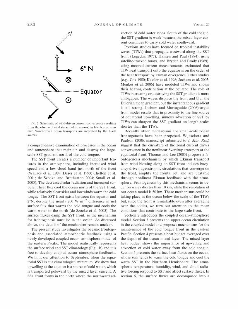
Our knowledge of eastern Pacific winds has im-proved substantially since the Cromwell (1953) study.In late boreal summer, southeasterlies prevail in theSouthern Hemisphere and cross the equator (Fig. 1a).North of the equator, the wind turns eastward and con-verges on the ITCZ north of 10°N. On the easternequator, the wind is directed northward parallel to theEcuadorian shore. Figure 2 is a schematic illustration ofcurrents generated by these winds. Veering wind gen-erates convergent Ekman current in the NorthernHemisphere. South of the equator, divergence of thecurrent results in upwelling of cold water, indicated inFig. 2 by the arrow out of the page. The wind drivescold water across the equator as far as 6°N where thewind is northward and Ekman transport is eastward.The SST front in Fig. 1b is considerably south of thewind-driven transport centered at 5°N. Hence the lineof convergence of the wind-driven current does not ex-plain the location of the SST front. This paper presents

1 The term “Ekman current” refers to a solution of the fric-tional Ekman model without pressure adjustment. “Wind-drivencurrent” is the generalized frictional current in the upper ocean.For finite Coriolis parameter f off the equator, the wind-drivencurrent approaches the Ekman current.

FIG. 1. (a) NOAA optimally interpolated SST (°C) for Septem-ber averaged over 1998–2003. Vectors show the SeptemberCOADS surface wind climatology. (b) IROAM 1998–2003 Sep-tember averaged SST (°C) and surface wind. The length of thearrow at the lower right is for a 10 m s�1 wind.

1 JUNE 2007 D E S Z O E K E E T A L . 2501

a comprehensive examination of processes in the oceanand atmosphere that maintain and destroy the large-scale SST gradient north of the cold tongue.

The SST front creates a number of important fea-tures in the atmosphere, including increased windspeed and a low cloud band just north of the front(Wallace et al. 1989; Deser et al. 1993; Chelton et al.2001; de Szoeke and Bretherton 2004; Small et al.2005). The decreased solar radiation and increased tur-bulent heat flux cool the ocean north of the SST front,while relatively clear skies and low winds warm the coldtongue. The SST front exists between the equator and2°N, despite the nearly 200 W m�2 difference in netsurface flux that warms the cold tongue and cools thewarm water to the north (de Szoeke et al. 2005). Thesurface fluxes damp the SST front, so the mechanismfor frontogenesis must lie in the ocean. As discussedabove, the details of the mechanism remain unclear.

The present study investigates the oceanic frontoge-nesis and associated atmospheric feedback using anewly developed coupled ocean–atmosphere model ofthe eastern Pacific. The model realistically representsthe surface wind and SST climatology (Fig. 1b) and it isfree to develop coupled ocean–atmosphere feedbacks.We limit our attention to September, when the equa-torial SST is at a climatological minimum. We show thatupwelling at the equator is a source of cold water, whichis transported poleward by the mixed layer current. ASST front forms in the north where the northward ad-

vection of cold water stops. South of the cold tongue,the SST gradient is weak because the mixed layer cur-rent continues to carry cold water southward.

Previous studies have focused on tropical instabilitywaves (TIWs) that propagate westward along the SSTfront (Legeckis 1977). Hansen and Paul (1984), usingsatellite-tracked buoys, and Bryden and Brady (1989),using moored current measurements, estimated thatTIW heat transport onto the equator is on the order ofthe heat transport by Ekman divergence. Other studies(e.g., Cox 1980; Kessler et al. 1998; Jochum et al. 2005;Menkes et al. 2006) have modeled TIWs and showntheir heating contribution at the equator. The role ofTIWs in creating or destroying the SST gradient is moreambiguous. The waves displace the front and blur theEulerian mean gradient, but the instantaneous gradientis still strong. Jochum and Murtugudde (2006) arguefrom model results that in proximity to the line sourceof equatorial upwelling, sinuous advection of SST byTIWs can sharpen the SST gradient on length scalesshorter than the TIWs.

Recently other mechanisms for small-scale oceanfrontogenesis have been proposed. Wijesekera andPaulson (2006, manuscript submitted to J. Mar. Res.)suggest that the curvature of the zonal current drivesconvergence in the nonlinear Sverdrup transport at theequatorial front. Thomas and Lee (2005) propose a fr-ontogenesis mechanism by which Ekman transportfrom wind blowing along an SST front induces buoy-ancy-driven ageostrophic circulations that converge onthe front, amplify the frontal jet, and are unstablethrough nonlinear Ekman feedback with the atmo-sphere. Frontogenesis by this mechanism seems to oc-cur on scales shorter than 10 km, while the resolution ofour ocean model is 50 km. These mechanisms could betaking place in the ocean below the scale of the TIWsbut, since the front is remarkable even after averagingover the eddies, we turn our attention to the meanconditions that contribute to the large-scale front.

Section 2 introduces the coupled ocean–atmospheremodel. Section 3 presents the upper-ocean circulationin the coupled model and proposes mechanisms for themaintenance of the cold tongue front in the easternPacific. Section 4 presents a heat budget averaged overthe depth of the ocean mixed layer. The mixed layerheat budget shows the importance of upwelling andadvection of cold water away from the cold tongue.Section 5 presents the surface heat fluxes on the ocean,whose sum tends to warm the cold tongue and cool thewarm SST in the Northern Hemisphere. The atmo-spheric temperature, humidity, wind, and cloud radia-tive forcing respond to SST and affect surface fluxes. Insection 6, the surface fluxes are decomposed into a

FIG. 2. Schematic of wind-driven current convergence resultingfrom the observed wind stress (white arrows) in late boreal sum-mer. Wind-driven ocean transports are indicated by the blackarrows.


component that depends solely on the SST and a com-ponent that is due to the atmospheric adjustment as itblows across the SST front. Section 7 summarizes ourfindings.

2. A coupled model of the eastern tropical Pacificregion

The International Pacific Research Center (IPRC)Regional Ocean Atmosphere Model (IROAM: Xie etal. 2007) simulates coupled ocean–atmosphere pro-cesses in the eastern Pacific Ocean. The IROAM con-sists of the Geophysical Fluid Dynamics LaboratoryModular Ocean Model version 2 (MOM2: Pacanowski1995), for the Pacific basin from 35°S to 35°N, coupledto the IPRC Regional Atmospheric Model (RAM:Wang et al. 2003) from 150° to 30°W between 35°S and35°N. Surface winds, humidity, temperature, and radia-tive fluxes over the western part of the Pacific Oceanare prescribed by the daily National Centers for Envi-ronmental Prediction–National Center for Atmo-spheric Research (NCEP–NCAR) reanalysis (Kistler etal. 2001), and turbulent fluxes are computed from abulk formula (Fairall et al. 2003). The lateral bound-aries of the RAM are nudged toward four-times dailyNCEP–NCAR reanalysis. The influence of the landsurface of the Americas is modeled by the Biosphere–Atmosphere Transfer Scheme (BATS: Dickinson et al.1993), and the SST of the Atlantic Ocean is prescribedto the RAM from the weekly Reynolds et al. (2002)optimally interpolated SST. The ocean and the atmo-sphere models have horizontal resolution of 0.5° � 0.5°.The MOM2 has 30 z-coordinate levels, 15 between thesurface and 200 m. MOM2 uses a constant lateral dif-fusivity of heat and momentum of 200 m2 s�1. Verticalmixing is computed with the Pacanowski and Philander(1981) parameterization, with a minimum vertical dif-fusivity of 10�6 m2 s�1. Overturning of unstable watercolumns is achieved by the Cox (1984) explicit convec-tion scheme.

The MOM2 is initialized with Levitus (1982) clima-tology in January 1991, spun up for five years withNCEP boundary conditions, and then coupled to theRAM in January 1996. Fluxes of heat and momentumare computed every time step by the RAM using theCoupled Ocean–Atmosphere Response Experiment(COARE: Fairall et al. 2003) bulk flux algorithm. Heatand momentum fluxes are averaged daily and updateddaily to the MOM2, and the SST is updated daily to theRAM.

We allow the coupled IROAM to spin up for twoyears before analyzing the output. IROAM “climatol-ogy” is averaged for each calendar month for the six

years 1998–2003. This period excludes the strong ElNiño of 1997. The results are changed little by extend-ing the average over 1997.

Figure 1b shows the IROAM September climatologyof SST and wind vectors in the eastern Pacific. The SSTpattern is quite similar to the NOAA optimally inter-polated SST (Fig. 1a). The strength and westward ex-tent of the cold tongue and the temperature of the coldupwelled water off the South American coast are real-istic. The SST front is stronger to the east in both theobservations and the model. The 26°C isotherm shiftsnorthward unrealistically at 100°W in the model, westof which the cold tongue front is more diffuse thanobserved.

The IROAM wind is similar to observations. Themodeled wind speed has a minimum over the coldtongue, but is too strong by 1–2 m s�1 compared toobservations. The modeled winds are stronger in theNorthern Hemisphere and more westerly in the ITCZthan observed. These wind errors could be related to anoverestimate of ITCZ precipitation (Xie et al. 2007),especially along the southwest coast of CentralAmerica.

3. Coupled simulation of the equatorial coldtongue with IROAM

Figure 3a shows the currents in the top grid layer ofthe ocean model (0–10 m). South of 3°N the westwardSouth Equatorial Current (SEC) is evident. The east-ward North Equatorial Countercurrent (NECC) isnorth of 5°N. In IROAM, west of 110°W, northwardcurrents exceeding 60 cm s�1 feed the southern flank ofthe NECC. Observations of surface currents (Johnsonet al. 2001) show that the maximum meridional currentaveraged between 170° and 95°W is only 13 cm s�1 at4°N. [The central Pacific average, appearing in Johnsonet al., has nearly easterly wind stress and more symmet-ric overturning about the equator than the eastern Pa-cific. The observation closest to the surface is at 20-mdepth; the surface current is extrapolated from the cur-rent observations at 20–30-m depth, so may not accu-rately represent the surface current.]

Such strong northward surface currents are not gen-erated when the MOM2 is forced by the NCEP surfacewind (not shown). The NCEP cross-equatorial wind isknown to be weaker than observed, especially in Sep-tember (Wu and Xie 2003). Nevertheless, the IROAMwind speed is about 1–2 m s�1 too strong. The strongnorthward current in the coupled IROAM is the Ek-man response to the stronger-than-observed windstress. West of 100°W the northward current inIROAM displaces the 26°C isotherm 1°–2° north rela-tive to observations.


The classical Ekman and geostrophic solutions arenot valid on the equator. Therefore, we analyze nu-merical solutions of the primitive equations fromIROAM. Without theoretical rigor, we describe thequalitative likeness of the numerical solutions to Ek-man and geostrophic idealizations.

Fronts will develop in the presence of meridional gra-dients and meridional current convergence. The east-ward turning of the wind between the equator and the

ITCZ drives convergent Ekman transport. The turningof the surface current results in a band of meridionalconvergence at 3°–6°N, shown by the shaded contoursin Fig. 3a. The convergence at 3°–6°N in Fig. 3a is northof the strongest SST gradient. The SST gradient is rela-tively weak at 5°N and strongest between the equatorand 2°N, where the surface current is weakly divergent.

A deeper look reveals that the surface current is notrepresentative of current throughout the surface mixedlayer. Rather, there is considerable shear in an isother-mal layer. Hereafter we refer to this isothermally mixedlayer simply as the “mixed layer” even though momen-tum is not mixed in the layer. A meridional–verticalcross section of the temperature and meridional currentfor the upper 100 m of the IROAM ocean along 95°Wis shown in Fig. 4. There are 10 model layers betweenthe surface and 100 m. Gray shading shows tempera-ture, with cold water upwelling to the surface at theequator. The surface mixed layer is evident where tem-perature contours are nearly vertical. The meridionalgradient of SST is confined near the equator.

The meridional currents in Fig. 4 show a northwardlens at the surface centered at 2°N. This is consistentwith Ekman drift to the right of the westward windstress in the Northern Hemisphere. At the equator, inthe absence of rotation, the wind-driven drift is in thedirection of the northward wind stress. Below the sur-face, currents are strongly southward in the mixedlayer. In the Northern Hemisphere the southward flowis in geostrophic balance with the pressure gradientfrom the westward increase in the sea surface height(Johnson et al. 2001; Niiler et al. 2003; Maximenko andNiiler 2005). Geostrophic and wind-driven flow com-bine near the surface. North of 6°N the Ekman trans-port is southward. The southward currents affect thesurface temperature distribution by temperature advec-tion in the mixed layer.

Since vertical mixing occurs rapidly compared tohorizontal temperature advection in the mixed layer,we assume that temperature in the mixed layer is al-ways effectively mixed, and the vertical average of ve-locity in the mixed layer advects the mixed layer aver-age temperature �T�, where angle brackets represent avertical average from the surface to the depth of themixed layer. The mixed layer depth h is defined as thedepth at which the ocean temperature is 0.5°C coolerthan the surface temperature. The advection of coldequatorial water by the northward surface currentabove warm water from the southward current (Fig. 4)causes unstable stratification and vertical overturningwhere the water masses meet at 1°–3°N. An internaltally of the heat source in the top 50 m of the modelshows that convective overturning is responsible for in-

FIG. 3. (a) IROAM SST (contours: °C) and surface current u0

vectors. The meridional convergence is shaded above 5 � 10�6

s�1. (b) Mixed layer depth h (contour interval: 10 m) and mixedlayer averaged velocity �u�. (c) Mixed layer–surface current dif-ferences (cm s�1, shaded).


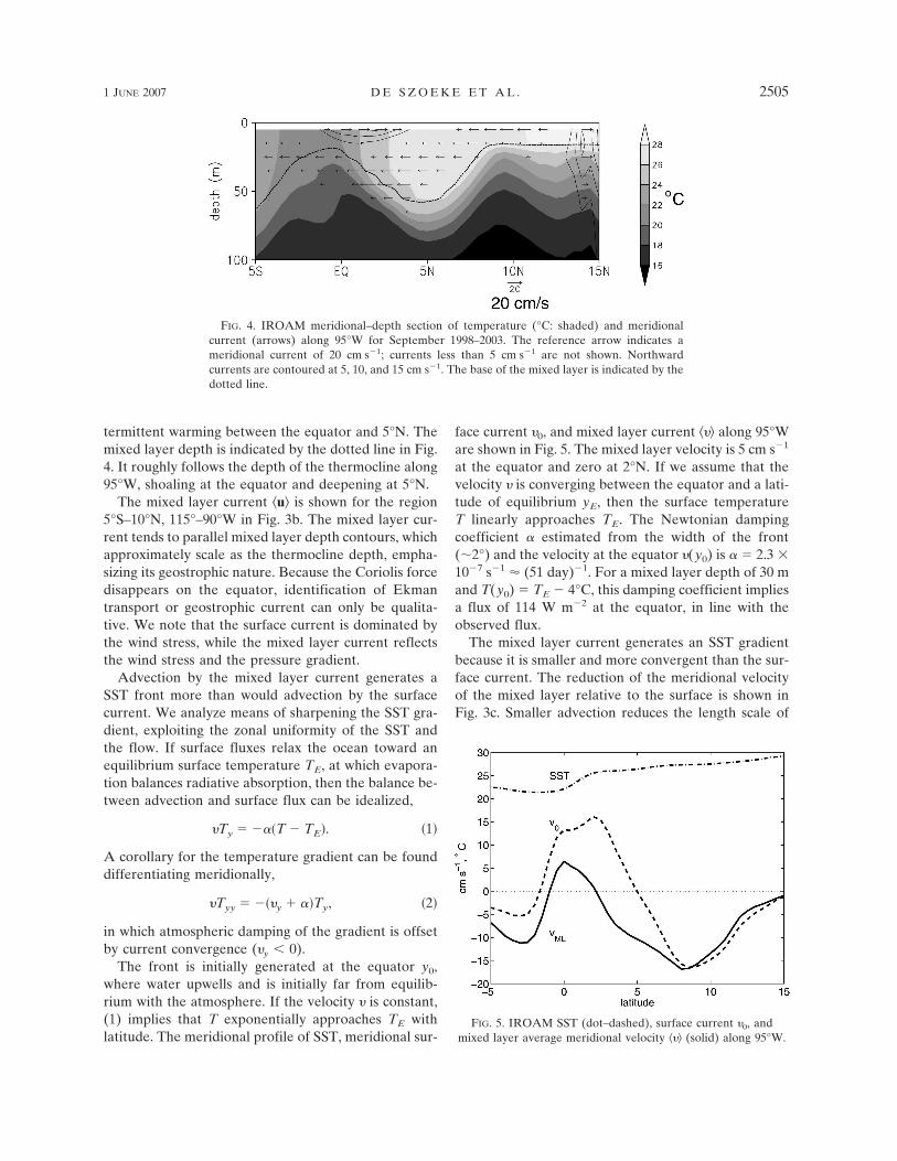
termittent warming between the equator and 5°N. Themixed layer depth is indicated by the dotted line in Fig.4. It roughly follows the depth of the thermocline along95°W, shoaling at the equator and deepening at 5°N.

The mixed layer current �u� is shown for the region5°S–10°N, 115°–90°W in Fig. 3b. The mixed layer cur-rent tends to parallel mixed layer depth contours, whichapproximately scale as the thermocline depth, empha-sizing its geostrophic nature. Because the Coriolis forcedisappears on the equator, identification of Ekmantransport or geostrophic current can only be qualita-tive. We note that the surface current is dominated bythe wind stress, while the mixed layer current reflectsthe wind stress and the pressure gradient.

Advection by the mixed layer current generates aSST front more than would advection by the surfacecurrent. We analyze means of sharpening the SST gra-dient, exploiting the zonal uniformity of the SST andthe flow. If surface fluxes relax the ocean toward anequilibrium surface temperature TE, at which evapora-tion balances radiative absorption, then the balance be-tween advection and surface flux can be idealized,

�Ty � ��T � TE�. �1�

A corollary for the temperature gradient can be founddifferentiating meridionally,

�Tyy � ��y � ��Ty, �2�

in which atmospheric damping of the gradient is offsetby current convergence (y 0).

The front is initially generated at the equator y0,where water upwells and is initially far from equilib-rium with the atmosphere. If the velocity is constant,(1) implies that T exponentially approaches TE withlatitude. The meridional profile of SST, meridional sur-

face current 0, and mixed layer current �� along 95°Ware shown in Fig. 5. The mixed layer velocity is 5 cm s�1

at the equator and zero at 2°N. If we assume that thevelocity is converging between the equator and a lati-tude of equilibrium yE, then the surface temperatureT linearly approaches TE. The Newtonian dampingcoefficient � estimated from the width of the front(�2°) and the velocity at the equator (y0) is � � 2.3 �10�7 s�1 (51 day)�1. For a mixed layer depth of 30 mand T(y0) � TE � 4°C, this damping coefficient impliesa flux of 114 W m�2 at the equator, in line with theobserved flux.

The mixed layer current generates an SST gradientbecause it is smaller and more convergent than the sur-face current. The reduction of the meridional velocityof the mixed layer relative to the surface is shown inFig. 3c. Smaller advection reduces the length scale of

FIG. 5. IROAM SST (dot–dashed), surface current 0, andmixed layer average meridional velocity �� (solid) along 95°W.

FIG. 4. IROAM meridional–depth section of temperature (°C: shaded) and meridionalcurrent (arrows) along 95°W for September 1998–2003. The reference arrow indicates ameridional current of 20 cm s�1; currents less than 5 cm s�1 are not shown. Northwardcurrents are contoured at 5, 10, and 15 cm s�1. The base of the mixed layer is indicated by thedotted line.


adjustment in (1) and (2). Meridional mixed layer con-vergence in the front increases by �5 � 10�7 s�1 rela-tive to the surface, changing the sign of the convergence(shaded in Figs. 3a,b) in the eastern part of the front.The convergence difference causes the mixed layer cur-rent to sharpen the SST gradient by 0.08°C (° lati-tude)�1 day�1 more than the surface current at 100°W.

Ekman transport from the clockwise-turning windstress drives convergence at 4°–6°N. Absent equatorialupwelling, water from both sides of the convergence iswarm and does not form a front. Once TIWs grow tosignificant amplitude in the west, their cold cusps reach4°–6°N and curl around clockwise. South of the cuspsthe SST gradient reverses, with cold water to the north.Warm water converges meridionally from the sides andthe cold water descends. Our analysis cannot distin-guish whether the TIWs are causing convergence orresponding to the wind-driven convergence here.

The minimum SST south of the equator clearly cor-responds to divergence in the surface and mixed layervelocity. The SST front is located between the equatorand 2°N. While meridional surface velocity 0 diverges,mixed layer velocity �� converges between the equatorand 2°N. The difference between the surface and themixed layer current between the equator and 5°Nshows the importance of southward geostrophic flow inthe mixed layer. At 2°–3°N the northward mixed layervelocity stops and is met by southward velocity fromthe north.

4. A mixed layer heat budget

The SST front is located in a region of weak north-ward meridional current (Fig. 3b). In this section wecompute the mixed layer heat budget for September,which demonstrates the relative roles of horizontal ad-vection, upwelling, and surface turbulent and radiativeflux in maintaining the SST front. To first order up-welling in the cold tongue is balanced by solar heating.Horizontal advection enhances the front by warming itsnorth side.

The temperature tendency equation used by theocean model is

�T

�t� �u · �T � � · ��T� � ��CP��1

�R

�z� QE � QH.

�3�

The first term on the right-hand side is three-dimen-sional advection, the second is diffusion, and the third isconvergence of the net radiative heat flux. The oceanmodel has penetrative solar radiation and assumes thatsurface longwave radiation is entirely absorbed and

emitted at the top model layer. The evaporative andsensible heat fluxes also converge in the surface layer;QE is the temperature sink due to surface evaporationand QH is due to the sensible heat flux. The fluxes R, E,and H are all defined positive downward. The effect ofthe explicit convection scheme, which vertically redis-tributes heat to mix out buoyant instability, is appliedseparately from the temperature equation and is notconsidered here.

The terms in (3) are computed for each model gridcell from daily averaged temperature, velocity, diffusiv-ity, and surface flux. To compute the heat budget forthe ocean mixed layer, the terms in (3) are verticallyaveraged over the mixed layer depth h. The mixed layerdepth h: T(�h) � T(0) �0.5 is computed from the dailydata and then averaged over a month. The averagemixed layer depth h is taken to be a constant through-out each month. We expect the ignored explicit con-vection to have only a small effect on the verticallyintegrated budget. The September climatologies pre-sented are the average of six Septembers from 1998 to2003. We separate the advection

u · �T � u · �T � u� · �T�, �4�

into advection by the monthly mean and by the eddies,respectively, where the overline represents the monthlymean.

Figure 6a shows zonal advection of the mixed layermean temperature by the monthly mean zonal current.A zonal temperature gradient exists because the tem-perature front is zonally tilted (cf. Fig. 1) with warmertemperature to the east. The zonal tilt of the front isbecause the southerly component of the wind increasesto the east. The southerly wind component shifts thecenter of upwelling south of the equator. In the west,where the winds are more zonal, the center of upwellingis nearer the equator. The strong westward SouthEquatorial Current (SEC) in the SST front region ad-vects warm water from the east into the front regionwith warming of 1°–3°C month�1. Zonal advection isstrong enough to change the sign of the total horizontaladvection to warming north of the equator (Fig. 6).South of the equator the gradient is reversed and zonaladvection cools about half as strongly as meridionaladvection. The zonal advection and local SST gradientdo not necessarily imply advection of parcels all theway from the South American coast. Traveling at themean mixed layer current of �30 cm s�1, it would takemore than a month for water to traverse 10° of longi-tude in which time its temperature would likely bedamped by surface fluxes.

The September mixed layer mean meridional veloc-ity advects cold upwelled water from the equator into


the temperature front, cooling the front on its southernflank (Fig. 6b). The mean meridional current is rela-tively weak, but the temperature gradient is strong, re-sulting in a cooling comparable in magnitude to thezonal warming. Advection is strong because of the tem-perature gradient and acts to strengthen the gradient.North of the front there is weak warming from meanmeridional advection because of southward advectionby the mixed layer velocity. The zonal warming isshifted slightly to the north of the front, and the me-ridional cooling is shifted slightly to the south. Totalmean horizontal advection (Fig. 6f) enhances the SSTdifference across the front by 1.5°C month�1.

In the Southern Hemisphere, both zonal and meridi-

onal currents contribute to a broad region of cold ad-vection, with its peak (�0.05°C day�1) at 3°S. The con-tinuity of the southward meridional mixed layer currentinto the Southern Hemisphere spreads cold water fromthe upwelling far to the south (Fig. 3b). In the NorthernHemisphere, meridional currents are weak and the coldwater stays on the south side of the front.

Westward propagating tropical instability wavesform along the temperature front between the equatorand 5°N, 90°–115°W. Currents from these eddies me-ander north- and southward, advecting the SST front asthey go. One or two TIWs propagate past a given pointeach month. In daily realizations, TIWs start to meridi-onally displace the 25°C isotherm between 100° and

FIG. 6. IROAM sources to the mixed layer temperature budget in September: the (a) zonal and (b) meridionaltemperature advection in the mixed layer by the September mean current and temperature. (c) The total eddyadvection. (d) The contribution of upwelling (the sum of diffusion and mean vertical advection) to the mixed layertemperature. (e) The total surface heat source from evaporation, sensible heat flux, and radiation. (f) The meanhorizontal advection [sum of (a) and (b)]. For reference contours (interval 1°C) of mixed layer temperature �T� areoverlaid. In (c) the thin contours are temperature variance [0.5(°C)2].


Fig 6 live 4/C

105°W. TIWs grow as they propagate westward from100°W, as indicated by the variance of the temperature(thin black contours, Fig. 6c). Though the instanta-neous SST gradient is just as strong in the west, themeandering displacement of the SST front weakens theEulerian monthly mean SST gradient.

The effect of TIWs on the mixed layer heat budget iscaptured by the eddy term, which is the sum of allhorizontal and vertical temperature advection by theeddies. The eddies transport temperature across thefrontal region and warm the core of the cold tongue. At95°W there is a zonal band of warm advection along theequator and cold advection on the north side of thefront. The dipole of temperature advection by the ed-dies grows and shifts northward as the TIWs grow westof 100°W (Fig. 6c). There is a large warming (�0.2°Cday�1) from the equator to 2°N and a small cooling at5°N. Between the centers of warming and cooling, ed-dies weaken the mean SST gradient.

West of 100°W at 0°–2°N, mean meridional advec-tion cooling doubles, and zonal advection cools becausethe temperature gradient reverses in the SEC north ofthe equator. The total mean horizontal advection(0.1°C day�1, Fig. 6f) cancels half the eddy warming inthe front. Mean horizontal advection warms around5°N, partly compensating for the weakening of thefront by eddies. Although TIWs weaken the front in thewest, Fig. 6 does not suggest an entirely differentmechanism for the front.

The contribution of upwelling to the mixed layertemperature is shown in Fig. 6d. The negative flux oftemperature through the base of the mixed layer isachieved by a combination of vertical advection anddiffusion. Vertical advection passes cold water throughthe thermocline to turbulent diffusion in the mixedlayer. Small changes in the diagnosis of h will result ina compensation between vertical advection and diffu-sion with little effect on the net upwelling term. Up-welling generates a band of cooling north of the coldtongue core and south of the SST front. Here the SST,mixed layer depth, and thermocline depth are at a mini-mum. At 115°W, where winds are nearly easterly (Fig.1), the maximum cooling is along the equator. To theeast, the winds are more southerly, shifting the up-welling core slightly south of the equator. This south-ward shift of the upwelling is reflected in the southeast-ward tilt of the SST front. Despite the change in thewind direction, the SST front and upwelling are quitezonal and trapped on the equator. Upwelling cooling isbalanced by warming from horizontal advection andsurface fluxes (Fig. 7b). Around 5°N, there is warmingfrom vertical advection, indicating that warm water is

converging horizontally and displacing cold waterthrough the base of the mixed layer.

The total convergence of the radiative, latent, andsensible heat flux from the surface of the mixed layer isshown in Fig. 6e. There is strong surface warming of thecold tongue. The cold SST reduces turbulent heat fluxand relatively clear skies maximize the insolation of theocean. Warming from surface flux divergence is en-hanced by the shallow mixed layer along the equator.When surface flux is absorbed by a relatively shallowlayer, the heating is greater. The change in sign of thetotal surface heat convergence coincides with the SSTfront. The change in surface heating across the frontwould tend to reduce the front by 3°C month�1. Northof the front, evaporation dominates insolation and themixed layer loses heat to the atmosphere.

The patterns of diffusion, advection, and surfaceheating are all zonally oriented along the SST front andof comparable magnitude in the mixed layer heat bud-get. To synthesize the effect of all the terms in the heatbudget, we have averaged surface heating (radiationand turbulent flux divergence), advection by the mean,advection by eddies, and diffusion between 90° and100°W. The meridional profile of the mixed layer av-erage temperature budget is presented in Fig. 7b. Theupwelling term (dot–dashed) is the sum of diffusion

FIG. 7. The mixed layer heat budget averaged from 90° to100°W. (a) The mixed layer temperature �T� (solid) and depth h(dashed). (b) The budget terms: surface flux divergence (includingradiation; dashed), horizontal advection by the mean (solid gray),advection by eddies (thin black), and upwelling (the sum of dif-fusion and vertical advection; dot–dashed). (c) The sum of thesources (solid), the mixed layer temperature tendency (gray), andthe residual (dashed).


and mean vertical advection. Horizontal diffusion istwo orders of magnitude smaller than vertical diffusion.On the equator surface heat flux (dashed) and advec-tion by eddies (thin solid) are heating the mixed layer,while upwelling cools it. Meridional (zonal) advectioncools (warms) the mixed layer along the temperaturefront (Figs. 6a,b). The net effect is that the mean hori-zontal advection (Figs. 6f and 7b) is small over the coldtongue and gradually increases from the equator to0.05°C day�1 at 1.5°N. The mixed layer temperaturesources at the equator in Fig. 7b are in agreement withthose computed using TAO buoy observations on theequator at 110°W (Fig. 6 of Wang and McPhaden 1999).

The net surface flux follows the SST. Where SST islow, evaporation is small, and absorption of solar ra-diation causes a net warming. Where SST is high,evaporation increases and provides a net surface cool-ing to the ocean mixed layer. In this way surface fluxrestores the mixed layer temperature to an equilibriumat which evaporation balances solar absorption. Surfacewarming is very strong over the coldest water and de-creases across the front as evaporative cooling increasesover warmer SST beneath relatively cold and dry air.

The effect of eddies is to advect warm water into thecold tongue. Eddies warm the cold tongue by 0.05°Cday�1, consistent with the warming effect of TTWs asmodeled by Kessler et al. (1998; 0.05°C day�1), Jochumand Murtugudde (2006; 0.08°C day�1), and Menkes etal. (2006; 0.07°C day�1). The zonal average over 90°–100°W is in the region of TIW development. WhereTIWs reach a larger amplitude farther west, they mayplay a larger role in the heat budget. The eddies alsoweakly cool the warm water north and south of the coldtongue, especially on the north side where the tempera-ture front is sharper.

The eastern equatorial Pacific Ocean may be dividedinto three zonal regions based on the mixed layer tem-perature budget in Fig. 7b. In the cold tongue centeredat 0.5°S, surface flux warming—dominated by radiativewarming and to a lesser extent eddy warming—balanceupwelling of cold water. South of 2°S, mean horizontaladvection by the persistent southward current trans-ports water from the cold tongue southward. Advectionkeeps this southern region cooler than its counterpartin the Northern Hemisphere. Moderate net surface fluxbalances cold advection in the south. In the NorthernHemisphere the poleward transport is weak and theadvection of cold tongue water stops at the front. In thethird region, north of 2°N, warm horizontal advectionfrom the north and east balances net surface cooling.The front in the Northern Hemisphere marks theboundary at the northern limit of the transport of up-welled cold water.

Figure 7a shows the mixed layer temperature �T� anddepth h for reference. Figure 7c shows the sum of heatsources (black solid) in Fig. 7b and the tendency of themixed layer temperature (gray solid). The residual(dashed) is the warming unexplained by the sum of thesources. The residual is small except in the vicinity ofthe SST front. At the front there is residual warmingconsistent with the effect of buoyant convective over-turning from cold water overriding warm water andsurface flux cooling at the SST front. Meridional cur-rents become more equatorward with depth, as ob-served (Johnson et al. 2001), preventing cold waterfrom sliding beneath warm water. In this unusual wind-driven circulation, the wind pushes dense water in thedirection of light water, which acts to tilt density sur-faces into the vertical. [This wind-driven buoyancy fluxresembles the first step in the frontogenic instability ofThomas and Lee (2005), however the instability cannotexist in our model because the motion of the surfaceocean current relative to the wind is not included in thewind stress.]

5. Surface heat fluxes: An atmospheric feedback

Sections 2–4 demonstrate how mixed layer velocity isimportant for the advection of heat in the mixed layerand how meridional convergence in the mixed layercreates conditions favorable for sharpening the SSTgradient. This section investigates the atmosphericfeedback of surface heat fluxes on SST.

The total surface heat flux and its components for theIROAM September (1998–2003) along 90°–100°W areshown in Fig. 8. Positive fluxes in Fig. 8 warm the

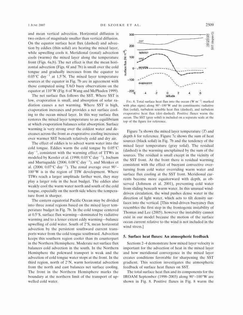
FIG. 8. Total surface heat flux into the ocean (W m�2: markedwith plus signs) along 90°–100°W and its constituents: radiativeflux (solid), turbulent sensible heat flux (dashed), and turbulentevaporative heat flux (dot–dashed). Positive fluxes warm theocean. The SST (gray solid) is included on a separate scale at thetop of the figure for reference.


ocean. The total heat flux into the ocean is 120 W m�2

over the cold tongue, dropping sharply to zero justnorth of 1°N. Strongest surface cooling of the oceanoccurs just to the warm side of the front at 2°–3°N andis a response to trade winds crossing the front. Evapo-ration, which varies with saturation specific humidity,relative humidity, and wind speed, is the main contribu-tor cooling the ocean. The cold advection in the atmo-sphere enhances cooling downwind of the SST front.

The net radiative heat flux into the ocean for Sep-tember is repeated in Fig. 9 (solid). The clear-sky ra-diative forcing is also shown. Under September equi-noctial conditions, clear-sky radiative forcing is rela-tively constant, around 230 W m�2. The clear-skyradiative forcing has a slight reduction north of the SSTfront where SST is warm and there is a thermal infrared“window” due to lack of water vapor in the atmo-sphere. The total radiative warming gradually shrinksnorth of the front as the cloud radiative forcing in-creases from �70 W m�2 over the cold tongue to �130W m�2 at 5°N. Cloud radiative forcing in IROAM de-clines southward between the equator and 5°S.IROAM, like many coupled general circulation models,underestimates tropical southeastern Pacific stratuscloudiness. Satellite observations show that clouds in-crease south of 2°S.

Clouds increase with cold PBL air blowing overwarm SST. The cold-advection PBL receives largemoisture and buoyancy fluxes from the warm oceansurface. Immediately north of the SST front, stratiformclouds condense in the PBL (Deser et al. 1993). Fromthe cold tongue to the ITCZ, stratiform clouds quicklygive way to cumulus under stratocumulus and then tocumulus clouds (Norris 1998) as the boundary layerdeepens over warming SST. This cloud transition was

observed in the East Pacific Investigation of Climate2001 experiment (EPIC: Raymond et al. 2004; Zeng etal. 2004; de Szoeke et al. 2005) and has previously beenmodeled with the IPRC Regional Atmospheric Model(Small et al. 2005) and with large eddy simulations (deSzoeke and Bretherton 2004).

From Fig. 8 the surface flux into the ocean is clearlylarger over the cold tongue than over the warmer waterto the north. The ocean surface temperature relaxestoward an equilibrium surface temperature TE at whichthe evaporation balances the radiative absorption (Xieand Seki 1997). The upwelled water is cold, so the heatfluxes are out of equilibrium with a deficit of evapora-tion and a surplus of radiative warming heating themixed layer. The water to the north is relatively wellequilibrated. In fact, the flux north of the front coolsthe ocean slightly because of cold atmospheric advec-tion from the south, warm oceanic advection from thenorth and the west, and negative cloud radiative forc-ing. The effect of adjustment of the PBL and clouds isexamined in the next section.

6. A surface heat flux decomposition

In this section we introduce a decomposition of thesurface turbulent heat flux. This decomposition dividesthe heat flux into a contribution from the ocean due tothe change in SST and a contribution from the atmo-sphere as it advects and adjusts across the front. Theocean contribution to the flux is similar to the flux pre-dicted by the Seager et al. (1988) model, which is oftenused as a thermodynamic boundary condition for oceangeneral circulation models.

The surface sensible heat flux H and evaporation Edepend on the product of several quantities in the bulkformula,

H � �CPCHU�T � Ta� �5�

E � �LCEU ��q*�T � � RHq*�Ta��, �6�

where � is the air density, CH and CE are bulk transfercoefficients for heat and moisture, CP is the specificheat of air, L is the latent heat vaporization of water, Uis the wind speed, T is the sea surface temperature, Ta

is the surface air temperature, RH is the relative hu-midity of the surface air, and q*(T) is the Wexler func-tion (or Clausius–Clapeyron relation) for the saturationspecific humidity of water as a function of temperature.The factor � � 0.98 parameterizes the reduction ofsaturation specific humidity over seawater relative tofreshwater. Let

�T � Ta � T �7�

FIG. 9. Net September IROAM radiative heat flux into theocean surface (solid) for 90°–100°W. The dashed line representsthe radiative heat flux for clear-sky conditions; the difference be-tween the total and the clear-sky flux is the cloud radiative forc-ing.


be the air–sea temperature difference, typically nega-tive 1°–2°C in the Tropics. We decompose it into meanand perturbation quantities,

�T � �T � �T�. �8�

The overbar mean represents a typical air–sea tempera-ture difference, which for the following analysis is de-fined simply as the mean over 5°S to 6°N.

The relative humidity of the atmosphere RH is usu-ally near 80%. In analogy to air–sea temperature dif-ference, relative humidity and wind speed are decom-posed RH � RH � RH�, and U � U � U�. The satu-ration specific humidity of the air can be decomposed:

q*�Ta� � q*�T � �T � � q*�T � �T � � q*� � q* � q*�.

�9�

Assuming constant air–sea temperature difference �T,saturation specific humidity over the ocean q* �q*(T � �T) depends only on the sea surface tempera-ture T and not on the air temperature Ta. The term q*�can be linearized about T � �T,

q*� ≅ �T��q*�T �

T��T. �10�

Cool atmospheric temperature anomalies increaseevaporation by decreasing q*�. The linearization intro-duces an error in the evaporation of less than 2% nearthe equatorial SST front, even where RH� and �T� arefar from equilibrium.

Having defined atmospheric mean and perturbationquantities, we decompose surface evaporation E (6)into three terms:

E � �LCEU ��q*�T � � RHq*� �i�

��LCEU��q*�T � � RHq*� �ii�

��LCEU ��RHq*� � RH�q*�Ta��, �iii�

represented by the separate equation lines (i)–(iii).Line (i) depends only on the ocean and the differencefrom the ocean of mean atmospheric quantities. Evenfor constant air–sea temperature difference �T andrelative humidity RH, variations in the ocean tempera-ture affect the evaporation because the saturation spe-cific humidity q*(T) is an exponential function of tem-perature. Lines (ii) and (iii) are forced by variations inthe atmosphere. Line (ii) depends only on wind speedperturbations U� and the ocean temperature T. Thethermodynamic atmospheric forcing (iii) depends onthe full wind speed U, the perturbation air–sea tem-perature difference �T�, and the perturbation relativehumidity RH�.

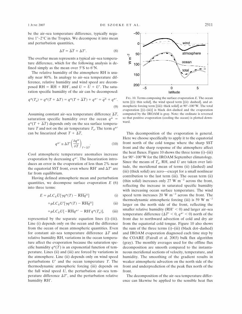
This decomposition of the evaporation is general.Here we choose specifically to apply it to the equatorialfront north of the cold tongue where the sharp SSTfront and the sharp response of the atmosphere affectthe heat fluxes. Figure 10 shows the three terms (i)–(iii)for 90°–100°W for the IROAM September climatology.Since the means of Ta, RH, and U are taken over lati-tude, the meridional mean of terms (ii) (dashed) and(iii) (thick solid) are zero—except for a small nonlinearcontribution to the last term (iii). The ocean term (ii)(thin solid) increases only 27 W m�2 across the front,reflecting the increase in saturated specific humiditywith increasing ocean surface temperature. The windspeed term increases 20 W m�2 across the front. Thethermodynamic atmospheric forcing (iii) is 59 W m�2

larger on the north side of the front, reflecting thesmaller relative humidity (RH� 0) and larger air–seatemperature difference (�T� 0, q*� 0) north of thefront due to northward advection of cold and dry airfrom the equatorial cold tongue. Figure 10 also showsthe sum of the three terms (i)–(iii) (black dot–dashed)and IROAM evaporation diagnosed each time step bythe COARE (Fairall et al. 2003) bulk flux algorithm(gray). The monthly averages used for the offline fluxdecomposition are smooth compared to the instanta-neous meridional sections of velocity, temperature, andhumidity. The smoothing of the gradient results inweaker atmospheric advection on the north side of thefront and underprediction of the peak flux north of thefront.

The decomposition of the air–sea temperature differ-ence can likewise be applied to the sensible heat flux

FIG. 10. Terms composing the surface evaporation E. The oceanterm [(i): thin solid], the wind speed term [(ii): dashed], and at-mospheric forcing term [(iii): thick solid] at 90°–100°W. The totalevaporation [(i)–(iii)] is black dot–dashed and the evaporationcomputed by the IROAM is gray. Note: the ordinate is reversedso that positive evaporation (cooling the ocean) is plotted down-ward.


(not shown). The sensible heat flux depends linearly onthe air–sea temperature difference �T, so the contribu-tion from the mean is uniform over the region. The heatflux out of the ocean increases 28 W m�2 across thefront due to the atmospheric adjustment �T� and in-creases 2 W m�2 due to the wind-driven component ofthe heat flux.

Table 1 shows the difference of the surface flux com-ponents between the cold tongue core and north of thefront (1°S–2.5°N). The surface flux components are theocean response to the change in the SST (Eocean), theeffect of the relative humidity, air temperature, andwind speed on the evaporation (Eatm), their effect onthe sensible heat flux (Hatm), and the net radiative fluxat the surface (R0). All four terms in Table 1 contributesignificantly to the surface flux difference across thefront. The largest contributor is Eatm, the evaporationdue to the cold, dry, and windy atmospheric anomalynorth of the front.

7. Summary

Setting aside seasonal and interannual variability, wehave described the conditions in the ocean mixed layerthat maintain the sharp SST front north of the easternPacific cold tongue in September. We have diagnosedreasons for the strength and location of the SST frontfrom IROAM, a coupled regional ocean–atmospheremodel.

The relative roles of ocean dynamics, the response ofthe surface flux to SST, and the atmospheric feedbackto the surface flux is summarized by Fig. 11. The oceandynamics term (gray) is the sum of all advection anddiffusion in the mixed layer—upwelling, horizontal ad-vection, and eddy advection from Fig. 7. The ocean fluxterm (black dashed) includes the contribution of theSST to the evaporation through the saturation specifichumidity, the mean sensible heat flux, and the net clear-sky radiative flux. The term from the atmosphere(black solid) includes the contribution to evaporationand sensible heat flux of departures in relative humid-ity, air–sea temperature difference, and wind speedfrom their typical values. The atmospheric forcing also

includes the cloud radiative forcing. The uniform offsetof the ocean flux and the atmospheric flux terms isarbitrary and occurs because the radiative absorption isalways positive, while the cloud radiative forcing is al-ways negative.

Cold water wells up near the equator and advectionand eddies distribute the cooling poleward. In thenorth, 40 W m�2 warm advection by the mean abuts thenorth edge of the SST front and cold water is held closeto the equator. In the Southern Hemisphere currentstransport cold water southward, resulting in cold advec-tion of 50–90 W m�2. The ocean flux changes 40 W m�2

in response to the SST change and clear-sky radiativeforcing across the front. The dynamical ocean heatsource is mostly compensated by atmospheric adjust-ment of the surface flux, which changes 150 W m�2

across the front. Cooling due to cloud radiative forcing,which gradually increases to the north, contributes al-most half of the atmospheric cooling across the front inIROAM.

The SST front forms fundamentally as the boundarybetween cold, recently upwelled, water and warm waterto the north, which has been in contact with strongtropical sunlight for a long time. The temperature at thesurface reflects the temperature of a thermally mixedlayer tens of meters deep. Within this mixed layer in thevicinity of the front there is mean vertical shear of themeridional current of 0.01 s�1. The wind-driven surfaceflow is northward. Below the surface there is southwardflow in response to the pressure gradients set up in theequatorial adjustment to the wind. This southward flow

TABLE 1. Components of the heat flux difference (W m�2) from1°S to 2.5°N: ocean forcing of the evaporation Eocean, total atmo-spheric forcing of the evaporation Eatm, sensible heat flux Hatm,and net downwelling radiation at the surface R.

Heat flux difference across 1°S–2.5°N

Eocean Eatm Hatm R Total

27 79 30 42 178

FIG. 11. A summary of important terms in the eastern tropicalPacific Ocean mixed layer heat budget. The ocean dynamical term(gray solid) is the sum of all advection and diffusion in the mixedlayer. The ocean flux (dashed) contains the contribution to theheat flux that depends on SST and the clear-sky radiative warm-ing. The atmosphere term (black solid) includes the contributionof departures from the mean air–sea temperature difference, rela-tive humidity, and wind speed, and the cloud radiative forcing.


contributes to the mean mixed layer velocity, movingthe line of meridional convergence equatorward from5° to 2°N and confining the meridional cold advectionclose to the equator. Owing to the orientation of thewind across the equator, the SST front is tilted north-west–southeast. The front is sharpened by zonal warmadvection on its north side by the northern branch ofthe westward SEC.

In the Southern Hemisphere water from the coldtongue is advected southward by the meridional cur-rent. Meridional cold advection is reinforced by coldadvection from the east by the SEC. Due to the con-tinuous extension of cold advection, the SST gradient isweaker in the Southern Hemisphere.

Though the focus of this study has been on the meanconditions that maintain the SST front, the role oftropical instability waves is included in the eddy term ofthe mixed layer heat budget. The effect of eddies is towarm the cold tongue core and weakly to cool the front.A study of the heat budget of tropical instability wavesby Jochum and Murtugudde (2006) shows that ratherthan mixing SST on diffusive scales, the waves spreadcold water poleward by oscillatory advection, therebyallowing the surface flux to heat the ocean more effi-ciently. An IROAM simulation that damps eddies byincreasing the lateral mixing (not shown) results in abroader and slightly colder cold tongue.

The surface sensible and evaporative heat flux hasbeen decomposed into two terms: an oceanic term thatresponds identically to SST anywhere over the oceanand an atmospheric term that reflects departures of theatmospheric temperature, humidity, and wind speedfrom equilibrium with the ocean surface. The decom-position attributes the maximum ocean cooling seen onthe north side of the front to strong advection of colddry air across the SST front. This advection leads tostrong evaporative and sensible cooling of the ocean.Positive wind speed anomalies further enhance evapo-ration and sensible heat flux north of the front. Thedecomposition of sensible heat flux and evaporationare general and can be performed on larger regions ofthe oceans of the globe. We expect the decompositionto yield similar results to the eastern Pacific equatorialfront in regions of atmospheric cold advection, wherestrong heat fluxes cool the ocean.

Acknowledgments. We would like to acknowledgethe insightful comments of Hyodae Seo, Billy Kessler,and two anonymous reviewers. This work has beenfunded by the Japanese Ministry of Education, Culture,Sports, Science and Technology (MEXT) as category 7of the RR2002 Project. The numerical calculation wascarried out at the Earth Simulator Center. The authors

wish to acknowledge the support of the U.S. NationalOceanic and Atmospheric Administration (NOAA)and the Japan Agency for Marine-Earth Science andTechnology (JAMSTEC). We acknowledge MichaelMcPhaden for his useful comments, and Sharon De-Carlo, Yingshuo Shen, and Kazutoshi Horiuchi, whohave diligently maintained our access to the IROAMdata. COADS data can be downloaded from theICOADS Web site (http://icoads.noaa.gov/) or the AsiaPacific Data Research Center Web site (http://apdrc.soest.hawaii.edu/).

REFERENCES

Bryden, H. L., and E. C. Brady, 1989: Eddy momentum and heatfluxes and their effect on the circulation of the equatorialPacific Ocean. J. Mar. Res., 47, 55–79.

Chelton, D. B., and Coauthors, 2001: Observations of couplingbetween surface wind stress and sea surface temperature inthe eastern tropical Pacific. J. Climate, 14, 1479–1498.

Cox, M. D., 1980: Generation and propagation of 30-day waves ina numerical model of the Pacific. J. Phys. Oceanogr., 10,1168–1186.

——, 1984: A primitive equation, 3-dimensional model of theocean. GFDL Ocean Group Tech. Rep. 1, 143 pp.

Cromwell, T., 1953: Circulation in the meridional plane in thecentral equatorial Pacific. J. Mar. Res., 12, 196–213.

Deser, C., S. Wahl, and J. J. Bates, 1993: The influence of seasurface temperature gradients on stratiform cloudiness alongthe equatorial front in the Pacific Ocean. J. Climate, 6, 1172–1180.

de Szoeke, S. P., and C. S. Bretherton, 2004: Quasi-Lagrangianlarge eddy simulations of cross-equatorial flow in the eastPacific atmospheric boundary layer. J. Atmos. Sci., 61, 1837–1858.

——, ——, N. A. Bond, M. F. Cronin, and B. M. Morley, 2005:EPIC 95°W observations of the eastern Pacific atmosphericboundary layer from the cold tongue to the ITCZ. J. Atmos.Sci., 62, 426–442.

Dickinson, R. E., A. Henderson-Sellers, and P. J. Kennedy, 1993:Biosphere-Atmosphere Transfer Scheme (BATS) version 1as coupled to the NCAR Community Climate Model. NCARTech. Note TN-387�STR, 80 pp.

Fairall, C. W., E. F. Bradley, J. E. Hare, A. A. Grachev, and J. B.Edson, 2003: Bulk parameterization of air–sea fluxes: Up-dates and verification for the COARE algorithm. J. Climate,16, 571–591.

Gill, A. E., 1980: Some simple solutions for heat-induced tropicalcirculation. Quart. J. Roy. Meteor. Soc., 106, 447–462.

Hansen, D. V., and C. A. Paul, 1984: Genesis and effects of longwaves in the equatorial Pacific. J. Geophys. Res., 89, 10 431–10 440.

Jochum, M., and R. Murtugudde, 2006: Temperature advection bytropical instability waves. J. Phys. Oceanogr., 36, 592–605.

——, ——, R. Ferrari, and P. Malanotte-Rizzoli, 2005: The impactof horizontal resolution in the tropical heat budget in anAtlantic Ocean model. J. Climate, 18, 841–851.

Johnson, G. C., M. J. McPhaden, and E. Firing, 2001: EquatorialPacific Ocean horizontal velocity, divergence, and upwelling.J. Phys. Oceanogr., 31, 839–849.

Kessler, W. S., L. M. Rothstein, and D. Chen, 1998: The annual


cycle of SST in the eastern tropical Pacific, diagnosed in anocean GCM. J. Climate, 11, 777–799.

Kistler, R., and Coauthors, 2001: The NCEP–NCAR 50-Year Re-analysis: Monthly means CD-ROM and documentation. Bull.Amer. Meteor. Soc., 82, 247–267.

Legeckis, R., 1977: Long waves in the eastern equatorial PacificOcean: A view from a geostationary satellite. Science, 197,1179–1181.

Levitus, S. E., 1982: Climatological Atlas of the World Ocean.NOAA Prof. Paper 13, 173 pp. and 17 microfiche.

Lindzen, R. S., and S. Nigam, 1987: On the role of sea surfacetemperature gradients in forcing low-level winds and conver-gence in the tropics. J. Atmos. Sci., 44, 2418–2436.

Maximenko, N. A., and P. P. Niiler, 2005: Hybrid decade-meanglobal sea level with mesoscale resolution. Recent Advancesin Marine Science and Technology, 2004, N. Saxena, Ed.,PACON International, 55–59.

McCreary, J. P., 1985: Modeling equatorial ocean circulation.Annu. Rev. Fluid Mech., 17, 359–409.

Menkes, C. E. R., J. G. Vialard, S. C. Kennan, J.-P. Boulanger,and G. V. Madec, 2006: A modeling study of the impact oftropical instability waves on the heat budget of the easternequatorial Pacific. J. Phys. Oceanogr., 36, 847–865.

Neelin, J. D., 1989: On the interpretation of the Gill model. J.Atmos. Sci., 46, 2466–2468.

Niiler, P. P., N. A. Maximenko, and J. C. McWilliams, 2003: Dy-namically balanced absolute sea level of the global oceanderived from near surface velocity observations. Geophys.Res. Lett., 30, 2164, doi:10.1029/2003GL018628.

Norris, J. R., 1998: Low cloud type over the ocean from surfaceobservations. Part II: Geographical and seasonal variations.J. Climate, 11, 383–403.

Pacanowski, R. C., 1995: MOM 2 documentation: User’s guideand reference manual. Version 1.0, 232 pp.

——, and S. G. H. Philander, 1981: Parameterization of verticalmixing in numerical models of tropical oceans. J. Phys.Oceanogr., 11, 1443–1451.

Philander, S. G. H., and R. C. Pacanowski, 1981: The oceanicresponse to cross-equatorial winds (with application tocoastal upwelling in low latitudes). Tellus, 33, 201–210.

Raymond, D. J., and Coauthors, 2004: EPIC2001 and the coupledocean–atmosphere system of the tropical east Pacific. Bull.Amer. Meteor. Soc., 85, 1341–1354.

Reynolds, R. W., N. A. Rayner, T. M. Smith, D. C. Stokes, and W.Wang, 2002: An improved in situ and satellite SST analysisfor climate. J. Climate, 15, 1609–1625.

Seager, R., S. E. Zebiak, and M. A. Cane, 1988: A model of thetropical Pacific sea surface temperature climatology. J. Geo-phys. Res., 93, 1265–1280.

Small, R. J., S.-P. Xie, Y. Wang, S. K. Esbensen, and D. Vickers,2005: Numerical simulation of boundary layer structure andcross-equatorial flow in the eastern Pacific. J. Atmos. Sci., 62,1812–1830.

Thomas, L. N., and C. M. Lee, 2005: Intensification of oceanfronts by down-front winds. J. Phys. Oceanogr., 35, 1086–1102.

Wallace, J. M., T. P. Mitchell, and C. Deser, 1989: The influenceof sea-surface temperature on surface wind in the easternequatorial Pacific: Seasonal and interannual variability. J.Climate, 2, 1492–1499.

Wang, W., and M. J. McPhaden, 1999: The surface-layer heat bal-ance in the equatorial Pacific Ocean. Part I: Mean seasonalcycle. J. Phys. Oceanogr., 29, 1812–1831.

Wang, Y., O. L. Sen, and B. Wang, 2003: A highly resolved re-gional climate model (IPRC-RegCM) and its simulation ofthe 1998 severe precipitation event over China. Part I: Modeldescription and verification of simulation. J. Climate, 16,1721–1738.

Wu, R., and S.-P. Xie, 2003: On the equatorial Pacific surface windchanges around 1977: NCEP–NCAR reanalysis versusCOADS observations. J. Climate, 16, 167–173.

Xie, S.-P., 2004: The shape of continents, air-sea interaction, andthe rising branch of the Hadley circulation. The Hadley Cir-culation: Present, Past and Future, H. R Diaz and R. S. Brad-ley, Eds., Kluwer Academic, 121–152.

——, and M. Seki, 1997: Causes of the equatorial asymmetry insea surface temperature over the eastern Pacific. Geophys.Res. Lett., 24, 2581–2584.

——, and Coauthors, 2007: A regional ocean–atmosphere modelfor eastern Pacific climate: Toward reducing tropical biases.J. Climate, 20, 1504–1522.

Zeng, X., M. A. Brunke, M. Zhou, C. Fairall, N. A. Bond, andD. H. Lenschow, 2004: Marine atmospheric boundary layerheight over the eastern Pacific: Data analysis and modelevaluation. J. Climate, 17, 4159–4170.


Documents

What Maintains the SST Front North of the Eastern Pacific ... · What Maintains the SST Front North of the Eastern Pacific Equatorial Cold Tongue?* SIMON P. DE SZOEKE AND SHANG-PING