The density of expected persistencediagrams and its kernel based

estimationFrederic Chazal

(Joint work with Vincent Divol)

https ://team.inria.fr/datashape/

https ://geometrica.saclay.inria.fr/team/Fred.Chazal/

IPAM, Los Angeles - April 30, 2019

Geometry of Big Data

What is topological structure of data ?

Challenges :→ no direct access to topological/geometric information : need of intermediate

constructions (simplicial complexes) ;→ distinguish topological “signal” from noise ;→ topological information may be multiscale ;→ statistical analysis of topological information.

?

What is topological structure of data ?

Challenges :→ no direct access to topological/geometric information : need of intermediate

constructions (simplicial complexes) ;→ distinguish topological “signal” from noise ;→ topological information may be multiscale ;→ statistical analysis of topological information.

Topological Data Analysis (TDA)Persistent homology !

?

The classical TDA pipeline

∞

00

Data FiltrationPersistenthomology

Multiscale topol.structure

Topol.information

1. Build a multiscale topol. structure on topof data : filtrations.

2. Compute multiscale topol. signatures :persistent homology

3. Take advantage of the signature for fur-ther Machine Learning and AI tasks : Re-presentations of persistence

Representations ofpersistence

MachineLearning / AI

Filtrations of simplicial complexes

• A filtered simplicial complex (or a filtration) S built on top of a set X is a family(Sa | a ∈ R) of subcomplexes of some fixed simplicial complex S with vertex set Xs. t. Sa ⊆ Sb for any a ≤ b.

• More generaly, filtration = nested family of spaces.

Filtrations of simplicial complexes

• A filtered simplicial complex (or a filtration) S built on top of a set X is a family(Sa | a ∈ R) of subcomplexes of some fixed simplicial complex S with vertex set Xs. t. Sa ⊆ Sb for any a ≤ b.

• More generaly, filtration = nested family of spaces.

Example : Let (X, dX) be a metric space.• The Vietoris-Rips filtration is the filtered simplicial complexe defined by : fora ∈ R,

[x0, x1, · · · , xk] ∈ Rips(X, a)⇔ dX(xi, xj) ≤ a, for all i, j.

Rips

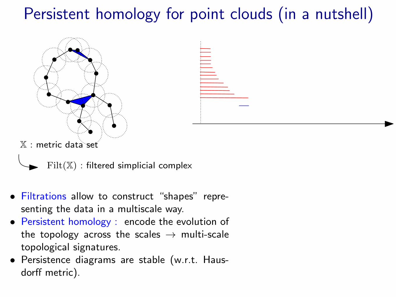
Persistent homology for point clouds (in a nutshell)

X : metric data set

• Filtrations allow to construct “shapes” repre-senting the data in a multiscale way.

• Persistent homology : encode the evolution ofthe topology across the scales → multi-scaletopological signatures.

• Persistence diagrams are stable (w.r.t. Haus-dorff metric).

Persistent homology for point clouds (in a nutshell)

X : metric data set

Filt(X) : filtered simplicial complex

• Filtrations allow to construct “shapes” repre-senting the data in a multiscale way.

• Persistent homology : encode the evolution ofthe topology across the scales → multi-scaletopological signatures.

• Persistence diagrams are stable (w.r.t. Haus-dorff metric).

Persistent homology for point clouds (in a nutshell)

X : metric data set

Filt(X) : filtered simplicial complex

• Filtrations allow to construct “shapes” repre-senting the data in a multiscale way.

• Persistent homology : encode the evolution ofthe topology across the scales → multi-scaletopological signatures.

• Persistence diagrams are stable (w.r.t. Haus-dorff metric).

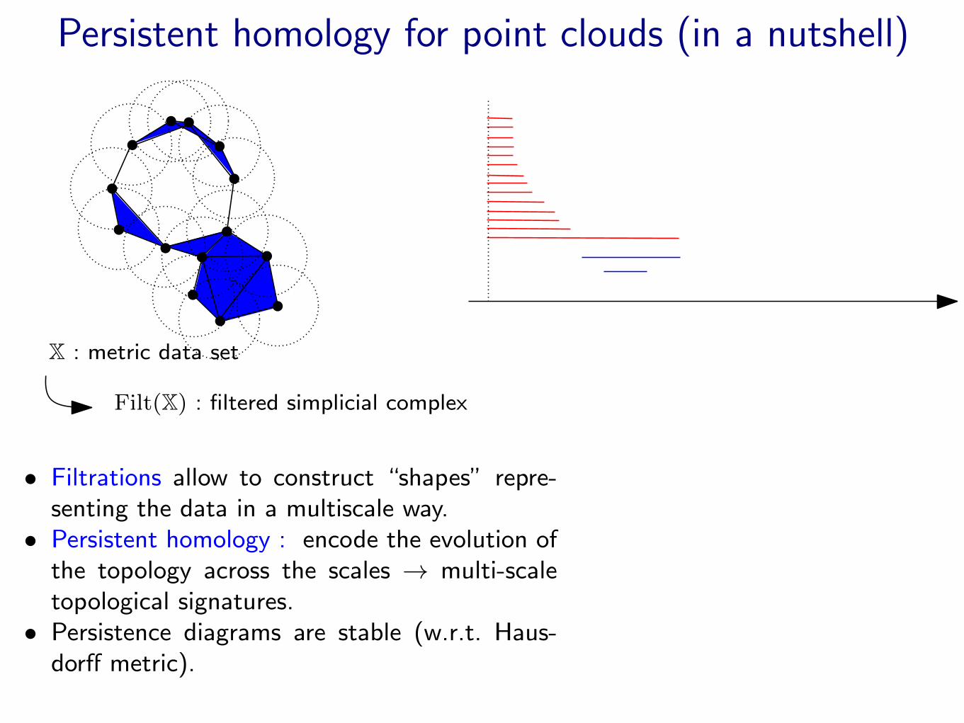
Persistent homology for point clouds (in a nutshell)

X : metric data set

Filt(X) : filtered simplicial complex

• Filtrations allow to construct “shapes” repre-senting the data in a multiscale way.

• Persistent homology : encode the evolution ofthe topology across the scales → multi-scaletopological signatures.

• Persistence diagrams are stable (w.r.t. Haus-dorff metric).

Persistent homology for point clouds (in a nutshell)

Persistence barcode

X : metric data set

Filt(X) : filtered simplicial complex

Persistence diagram

• Filtrations allow to construct “shapes” repre-senting the data in a multiscale way.

• Persistent homology : encode the evolution ofthe topology across the scales → multi-scaletopological signatures.

• Persistence diagrams are stable (w.r.t. Haus-dorff metric).

Persistent homology of filtered simplicial complexes

Let S = (Sa | a ∈ R) be a finite filtered simplicial complex with N simplices andlet Sa1 ⊂ Sa2 ⊂ · · · ⊂ SaN be the discrete filtration induced by the entering timesof the simplices : Sai \ Sai−1 = σai .

Persistent homology of filtered simplicial complexes

Let S = (Sa | a ∈ R) be a finite filtered simplicial complex with N simplices andlet Sa1 ⊂ Sa2 ⊂ · · · ⊂ SaN be the discrete filtration induced by the entering timesof the simplices : Sai \ Sai−1 = σai .

Process the simplices according to their order of entrance in the filtration :

Let k = dimσai

Persistent homology of filtered simplicial complexes

Let S = (Sa | a ∈ R) be a finite filtered simplicial complex with N simplices andlet Sa1 ⊂ Sa2 ⊂ · · · ⊂ SaN be the discrete filtration induced by the entering timesof the simplices : Sai \ Sai−1 = σai .

Process the simplices according to their order of entrance in the filtration :

Let k = dimσai

Case 1 : adding σai to Sai−1 creates anew k-dimensional topological featurein Sai (new homology class in Hk).

Sai−1

σai

⇒ the birth of a k-dim feature is registered.

Persistent homology of filtered simplicial complexes

Let S = (Sa | a ∈ R) be a finite filtered simplicial complex with N simplices andlet Sa1 ⊂ Sa2 ⊂ · · · ⊂ SaN be the discrete filtration induced by the entering timesof the simplices : Sai \ Sai−1 = σai .

Process the simplices according to their order of entrance in the filtration :

Let k = dimσai

Case 1 : adding σai to Sai−1 creates anew k-dimensional topological featurein Sai (new homology class in Hk).

Sai−1

σai

⇒ the birth of a k-dim feature is registered.

Case 2 : adding σai to Sai−1 kills a(k− 1)-dimensional topological featurein Sai (homology class in Hk−1).

Sai−1

σai

⇒ persistence algo. pairs the simplex σaito the simplex σaj that gave birth to thekilled feature.

Persistent homology of filtered simplicial complexesProcess the simplices according to their order of entrance in the filtration :

Let k = dimσai (ie. σai = [v0, · · · , vk])

Case 1 : adding σai to Sai−1 creates anew k-dimensional topological featurein Sai (new homology class in Hk).

Sai−1

σai

⇒ the birth of a k-dim feature is registered.

Case 2 : adding σai to Sai−1 kills a(k− 1)-dimensional topological featurein Sai (homology class in Hk−1).

Sai−1

σai

⇒ persistence algo. pairs the simplex σaito the simplex σaj that gave birth to thekilled feature.

(σaj , σai) : persistence pair

(aj , ai) ∈ R2 : point in thepersistence diagram

→→

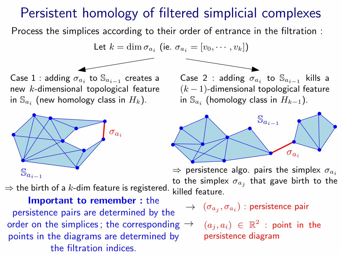
Persistent homology of filtered simplicial complexesProcess the simplices according to their order of entrance in the filtration :

Let k = dimσai (ie. σai = [v0, · · · , vk])

Case 1 : adding σai to Sai−1 creates anew k-dimensional topological featurein Sai (new homology class in Hk).

Sai−1

σai

⇒ the birth of a k-dim feature is registered.

Case 2 : adding σai to Sai−1 kills a(k− 1)-dimensional topological featurein Sai (homology class in Hk−1).

Sai−1

σai

⇒ persistence algo. pairs the simplex σaito the simplex σaj that gave birth to thekilled feature.

(σaj , σai) : persistence pair

(aj , ai) ∈ R2 : point in thepersistence diagram

→→

Important to remember : thepersistence pairs are determined by the

order on the simplices ; the correspondingpoints in the diagrams are determined by

the filtration indices.

Statistical setting

∞

00

X K(X)

D[K(X)]

X is a random pointcoud (in some metricspace)

K is a deterministicfiltration (e.g. Rips)

D[K(X)] becomesrandom

Statistical setting

∞

00

X K(X)

D[K(X)]

X is a random pointcoud (in some metricspace)

K is a deterministicfiltration (e.g. Rips)

D[K(X)] becomesrandom

What can be said about the distribution of diagrams D[K(X)] ?

Understand the structure of E[D[K(X)]] in the non asymptotic setting ( |X| =n is fixed, or bounded)

What does this mean ?

Persistence diagrams as discrete measures

D D :=∑r∈D

δr

• The space of measures is much nicer that the space of P. D. !• In the “standard” algebraic persistence theory, persistence diagrams

naturally appear as discrete measures in the plane (over rectangles).

• Many persistence representations can be expressed as

D(φ) =∑r∈D

φ(r) =

∫φ(r)dD(r)

for well-chosen functions φ.

Motivations :

[Chazal, de Silva, Glisse, Oudot 16]

Representation of Persistence diagrams

A representation is called linear if there exists φ : R2> → H such that

Φ(D) =∑r∈D

φ(r) := D(φ) =

∫φ(r) dD(r)

Persistent silhouette Persistent surface[Chazal & al, 2013] [Adams & al, 2016]

Distrib. of life span, totalpersistence,...

In ML settings, well-suited linear representations of PD can be learnt.[Hofer et al., NeurIPS 2017, Carriere et al, 2019]

Representation of Persistence diagrams

— D is a random persistence diagram— E[D] is a deterministic measure on R2

> defined by

∀A ⊂ R2>, E[D](A) = E[D(A)].

— D1, . . . , DN i.i.d.

Φ =Φ(D1) + · · ·+ Φ(DN)

N= µ(φ)

≈ E[D](φ)

E[D](φ) =

∫R2>

φ(r)p(r)d r ?

Does E[D] has a density w.r.t. Lebesgue measure in R2 ?

Estimation of p ?

The density of expected persistence diagrams

Theorem : Fix n ≥ 1. Assume that :

• M is a real analytic compact d-dimensional connected riemannian ma-nifold possibly with boundary,

• X is a random variable on Mn having a density with respect to theHaussdorf measure Hdn,

• K is the Vietoris-Rips filtration.

Then, for s ≥ 1, E[Ds[K(X)]] has a density with respect to the Lebesguemeasure on R2

>. Moreover, E[D0[K(X)]] has a density with respect to theLebesgue measure on the vertical line {0} × [0,∞).

The density of expected persistence diagrams

Theorem : Fix n ≥ 1. Assume that :

• M is a real analytic compact d-dimensional connected riemannian ma-nifold possibly with boundary,

• X is a random variable on Mn having a density with respect to theHaussdorf measure Hdn,

• K is the Vietoris-Rips filtration.

Then, for s ≥ 1, E[Ds[K(X)]] has a density with respect to the Lebesguemeasure on R2

>. Moreover, E[D0[K(X)]] has a density with respect to theLebesgue measure on the vertical line {0} × [0,∞).

Theorem [smoothness] : Under the assumption of previous theorem, if mo-reover X ∈ Mn has a density of class Ck with respect to Hnd. Then, fors ≥ 0, the density of E[Ds[K(X)]] is of class Ck.

Remark : This is a particular case of a much more general result.

The density of expected persistence diagrams

Idea of the proof :

• Standard arguments from real analytic geometry :up to a set of measure 0, Mn can be decomposed into a finite set ofopen sets Vi on which the order on the simplices induced by the Ripfiltration is constant.

• Classical argument from geometric measure theory (co-area formula) :the map from Vi to the space of PD has maximal rank and the imageof the random variable X has density with respect to Lebesgue measureon R2.

Filtrations revisited

Let n > 0 be an integer,Fn : the collection of non-empty subsets of {1, . . . , n},M : a real analytic compact d-dim. connected manifold (poss. with boundary).

Filtering function :

ϕ = (ϕ[J ])J∈Fn: Mn → R|Fn|

satisfiying the following conditions :

(K2) Invariance by permutation : For J ∈ Fn and for (x1, . . . , xn) ∈ Mn,if τ is a permutation of the entries having support included in J , thenϕ[J ](xτ(1), . . . , xτ(n)) = ϕ[J ](x1, . . . , xn).

(K3) Monotony : For J ⊂ J ′ ∈ Fn, ϕ[J ] ≤ ϕ[J ′].

Given x = (x1, · · · , xn), ϕ(x) induces an order on the faces of the simplexwith n vertices that is a filtration K(x) :

∀J ∈ Fn, J ∈ K(x, r)⇐⇒ ϕ[J ](x) ≤ r.

The case of the Vietoris-Rips filtration

ϕ[J ](x) = maxi,j∈J

d(xi, xj)

(K1) Absence of interaction : For J ∈ Fn, ϕ[J ](x) only depends on x(J).

(K2) Invariance by permutation : For J ∈ Fn and for (x1, . . . , xn) ∈ Mn,if τ is a permutation of the entries having support included in J , thenϕ[J ](xτ(1), . . . , xτ(n)) = ϕ[J ](x1, . . . , xn).

(K3) Monotony : For J ⊂ J ′ ∈ Fn, ϕ[J ] ≤ ϕ[J ′].

(K4) Compatibility : For a simplex J ∈ Fn and for j ∈ J , if ϕ[J ](x1, . . . , xn)is not a function of xj on some open set U of Mn, then ϕ[J ] ≡ϕ[J\{j}] on U .

(K5’) Smoothness : The function ϕ is subanalytic and the gradient of each ofits entries J of size larger than 1 is non vanishing a.e. and for J = {j},ϕ[{j}] ≡ 0.

Sketch of proof

1. There exists a partition of the complement of a (subanalytic) set ofmeasure 0 in Mn by open sets V1, · · · , VR such that :

• the order of the simplices of K(x) is constant on each Vr,• for any r = 1, · · · , R, and any x ∈ Vr,

Ds[K(x)] =

Nr∑i=1

δri

with ri = (ϕ[Ji1 ](x), ϕ[Ji2 ](x)) where Nr, Ji1 , Ji2 only depends onVr.

• Ji1 , Ji2 can be chosen so that the differential of

Φir : x ∈ Vr → ri = (ϕ[Ji1 ](x), ϕ[Ji2 ](x))

has maximal rank 2.

Sketch of proof

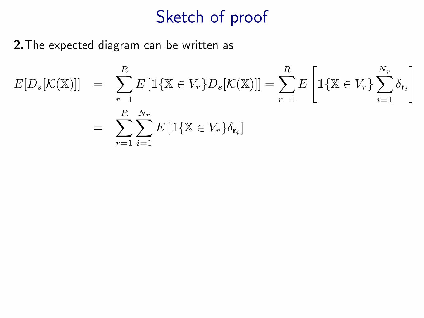
2.The expected diagram can be written as

E[Ds[K(X)]] =R∑r=1

E [1{X ∈ Vr}Ds[K(X)]] =R∑r=1

E

[1{X ∈ Vr}

Nr∑i=1

δri

]

=R∑r=1

Nr∑i=1

E [1{X ∈ Vr}δri ]

Sketch of proof

2.The expected diagram can be written as

E[Ds[K(X)]] =R∑r=1

E [1{X ∈ Vr}Ds[K(X)]] =R∑r=1

E

[1{X ∈ Vr}

Nr∑i=1

δri

]

=R∑r=1

Nr∑i=1

E [1{X ∈ Vr}δri ]

3. Use the co-area formula :

µir(B) = P (Φir(X) ∈ B,X ∈ Vr)

=

∫Vr

1{Φir(x) ∈ B}κ(x)dHnd(x)

=

∫u∈B

∫x∈Φ−1

ir (u)

(JΦir(x))−1κ(x)dHnd−2(x)du.

µir

Density of X

Density of µir

The Hausdorff measure and the co-area formula

Definition : Let k be a non-negative number. For A ⊂ RD, and δ > 0,consider

Hδk(A) := inf

{∑i

diam(Ui)k, A ⊂

⋃i

Ui and diam(Ui) < δ

}.

The k-dimensional Haussdorf measure on RD of A is defined by Hk(A) :=limδ→0Hδk(A).

Theorem [Co-area formula] : Let M (resp. N) be a smooth Riemannianmanifold of dimension m (resp n). Assume that m ≥ n and let Φ : M → Nbe a differentiable map. Denote by DΦ the differential of Φ. The Jacobianof Φ is defined by JΦ =

√det((DΦ)× (DΦ)t). For f : M → N a positive

measurable function, the following equality holds :∫M

f(x)JΦ(x)dHm(x) =

∫N

(∫x∈Φ−1({y})

f(x)dHm−n(x)

)dHn(y).

Persistence images[Adams et al, JMLR 2017]

For K : R2 → R a kernel and H a bandwidth matrix (e.g. a symmetricpositive definite matrix), pose for u ∈ R2, KH(z) = |H|−1/2K(H−1/2 · u)

For D =∑i δri a diagram, K : R2 → R a kernel, H a bandwidth matrix and

w : R2 → R+ a weight function, one defines the persistence surface of D withkernel K and weight function w by :

∀z ∈ R2, ρ(D)(u) =∑i

w(ri)KH(u− ri) = D(wKH(u− ·))

Persistence images[Adams et al, JMLR 2017]

For K : R2 → R a kernel and H a bandwidth matrix (e.g. a symmetricpositive definite matrix), pose for u ∈ R2, KH(z) = |H|−1/2K(H−1/2 · u)

For D =∑i δri a diagram, K : R2 → R a kernel, H a bandwidth matrix and

w : R2 → R+ a weight function, one defines the persistence surface of D withkernel K and weight function w by :

∀z ∈ R2, ρ(D)(u) =∑i

w(ri)KH(u− ri) = D(wKH(u− ·))

⇒ persistence surfaces can be seen as kernel based estimators of E[Ds[K(X)]].

Persistence images

The realization of 3different processes

The overlay of 40different persistence

diagrams

The persistence imageswith weight functionw(r) = (r2 − r1)3 and

bandwith selected usingcross-validation.

Thank you for your attention

Software :• GUDHI library C++ / Python : http ://gudhi.gforge.inria.fr/• R package TDA : Statistical Tools for Topological Data Analysis

References :

• F. Chazal, V. Divol, The density of expected persistence diagrams and its kernelbased estimation, SoCG 2018.