What is a structural representation?Second version∗

Lev Goldfarb, David Gay, Oleg Golubitsky, Dmitry Korkin

Faculty of Computer ScienceUniversity of New Brunswick

Fredericton, Canada

April 3, 2004

AbstractWe outline a formalism for “structural”, or “symbolic”, representation, the necessity

of which is acutely felt in all sciences. One can develop an initial intuitive understandingof the proposed representation by simply generalizing the process of construction ofnatural numbers: replace the identical structureless units out of which numbers arebuilt by several structural ones, attached consecutively. Now, however, the resultingconstructions embody the corresponding formative/generative histories, since we cansee what was attached and when.

The concept of class representation—which inspired and directed the developmentof this formalism—differs radically from the known concepts of class. Indeed, the evolv-ing transformation system (ETS) formalism proposed here is the first one developed tosupport that concept; a class representation is a finite set of weighted and interrelatedtransformations (“structural segments”), out of which class elements are built.

The formalism allows for a very natural introduction of representational levels: anext-level unit corresponds to a class representation at the previous level.

We introduce the concept of “intelligent process”, which provides a suitable sci-entific environment for the investigation of structural representation. This process isresponsible for the actual construction of levels and of representations at those levels;conventional “learning” and “recognition” processes are integrated into this process,which operates in an unsupervised mode. Together with the concept of structural rep-resentation, this leads to the delineation of a new field—inductive informatics—whichis intended as a rival to conventional information processing paradigms.

From the point of view of the ETS formalism, classical discrete “representations”(strings, graphs) now appear as incomplete special cases at best, the proper “com-pletion” of which should incorporate corresponding generative histories (e.g. those ofstrings or graphs).

∗ Technical Report TR04-165, Faculty of Computer Science, UNB. This paper is a substantially modifiedversion of [19].

1

[W]e may again recall what Einstein stressed: that given a sufficiently pow-erful formal assumption, a fertile and comprehensive theory may . . . beconstructed without prior attention to the detailed facts, or even beforethey are known.

L. L. Whyte, Internal Factors in Evolution, 1965

Part I

Prolegomenon[W]e are all waiting, not necessarily for a recipe, but for new techniques forapprehending the utterly remote past. Without such a breakthrough, wecan continue to reason, speculate, and argue, but we cannot know. Unlesswe acquire novel and powerful methods of historical enquiry, science willeffectively have reached a limit. [Emphasis added.]

F. M. Harold, The Way of the Cell, 2001

1 Introduction

1.1 Obstacles toward a formalism for structural representation

In this paper we outline a vision of the concept of structural representation which has beenin gestation for almost twenty years.

On the one hand, although the overwhelming importance of structural/symbolic repre-sentations in all sciences has become increasingly clear during the second half of the twentiethcentury, there have hardly been any systematic attempts to address this topic at a funda-mental level1. (This situation is particularly puzzling from the point of view of computerscience, in view of the central role played by “data structures” and “abstract data types”.)On the other hand, it is not that difficult to understand the main reasons behind this stateof affairs. From a theoretical point of view, it appears there are two very formidable ob-stacles to be cleared: 1) the choice of the central “intelligent” process, the structure andrequirements of which would both drive and justify the choice of a particular form of struc-tural representation, and 2) the lack of any fundamental mathematical models whose rootsare not directly related to numeric models. The order in which these obstacles must beaddressed is important: obviously, one must first choose which intelligent process to modelbefore attempting to look for a satisfactory formalism. Unfortunately, the second of theabove obstacles is usually underestimated or overlooked entirely.

1 The Chomsky formal grammar model will be discussed later in the Introduction. We are not aware ofany other (not derived from the Chomsky approach) basic attempts at structural/symbolic representation.

2

Why has it been overlooked? Because, during mankind’s scientific history, we have dealtonly with numeric models and, during the last century, with their derivatives. The lattershould not be surprising if we look carefully at the vast prehistory of science in general, and ofmathematics in particular [23], [35]. New mathematical abstractions and overspecializations(with a resulting narrowing of historical perspective) during the second half of the twentiethcentury have also contributed to such a lack of understanding of the extent to which wedepend on numeric models2. What has (barely) begun to facilitate this understanding,however, is the emergence of computer science in general, and artificial intelligence andpattern recognition (PR) in particular3.

The overwhelming preponderance of numeric models in science4 suggests that it is un-reasonable to expect a transition from numerically-motivated forms of representation, whichhave a millennia-old tradition behind them, to structural forms of representation to be ac-complished in one or several papers. At the same time, one should not try to justify, as isoften done in artificial intelligence, practically nonexistent progress in this direction by thecomplexity of the task.

1.2 Recent historical perspective: the need for unification

In this work, we outline a fundamentally new formalism—evolving transformation system(ETS)—which is the culmination of a research program originally directed towards the de-velopment of a unified framework for pattern recognition [11]–[18].

In view of the fact that newer, more fashionable “reincarnations” of PR (see footnote3) have missed what is probably the most important “representational” development withinPR during the 1960s and 1970s, we now touch on this issue (which actually motivated theoriginal development of the ETS framework). Over these two decades, it gradually becameclear to a number of leading researchers in PR that the two basic approaches to PR—theclassical vector-space-based, or statistical, approach and the syntactic/structural approach[9], each possessing the desirable features lacking in the other—should be unified [2]:

Thus the controversy between geometric and structural approaches for problem ofpattern recognition seems to me historically inevitable, but temporary. There areproblems to which the geometric approach is . . . suited. Also there are some wellknown problems which, though solvable by the geometric method, are more easilysolvable by the structural approach. But any difficult problems require a combinationof these approaches, and methods are gradually crystallizing to combining them; thestructural approach is the means of construction of a convenient space; the geometricis the partitioning in it.

Although these original expectations for an impending unification were quite high, itturned out that such hopes were naive, not so much with respect to timeliness but with

2 There are, of course, rare exceptions (see [36], for example).3 Although, for political reasons, during the last twenty years, several “new” areas very closely related

to PR appeared (such as machine learning, neural networks, etc), we will refer to them collectively by thename of the original area, i.e. pattern recognition, or occasionally as inductive learning.

4 For an insightful explanation of how the stage was set for this, see [7].

3

respect to the (underestimated) novelty of such a unified formalism: there was no formalframework which could naturally accommodate unification [11]. It is interesting to notethat researchers working in the various “reincarnations” of PR have only relatively recentlybecome aware of the need for, and of the difficulties associated with, such an effort. Thelarge number of conferences, workshops, and sessions devoted to “hybrid” approaches (e.g.[4], [38], [40], [41]) attests to the rediscovery of the need for unification.

1.3 The general approach we have taken

Returning to the two formidable obstacles mentioned in section 1.1, for us and many oth-ers the choice of the central intelligent process reduced to the pattern recognition process,or more accurately the pattern (or inductive) learning process5, with an emphasis on theinductive class representation. On the other hand, overcoming the second obstacle, i.e. thedevelopment of an appropriate mathematical formalism for modelling inductive processes,has been and will be a major undertaking.

What are some of the main difficulties we have encountered? In a roughly historicalorder, they are as follows. On which foundation should the unification of the above twobasic approaches to PR be approached? How do we formalize the concept of inductiveclass representation? How should the Chomsky concept of generativity be revised? How dowe generalize the Peano axiomatic construction of natural numbers to the construction ofstructural objects? In other words, how do we formally capture the more general inductive(or generative) process of object construction? What is the connection between a classdescription/representation and the process that generates class objects? How is an objectrepresentation connected to its class representation, and, moreover, how do these objectrepresentations change during the learning process? How do we introduce representationallevels and how do they communicate during the intelligent process? It is understood thatall of the above must be accomplished naturally within a single general model.

On the formal side, we chose the path of a far-reaching generalization of the Peano ax-iomatization/construction of natural numbers ([28] or [29]), the axiomatics that forms thevery foundation of the present construction of mathematics. This choice appears to be avery natural way to proceed. As well-known nineteenth-century German mathematician L.Kronecker aptly remarked, “God made the integers; all the rest is the work of man”. Thus, inpart, the original logic behind the formalization was this: take the only existing “representa-tional” model, natural numbers, and generalize the process of their construction/generation,i.e. replace the identical structureless primitives out of which natural numbers are built (Fig.8, p. 19) by various structural ones (Fig. 7, p. 18). Then, one can build on that foundation.

5 Inductive learning processes have been suggested as being the central intelligent processes by a numberof great philosophers and psychologists over the last several centuries (see, for example, [3], [22], [31]). Anexample of a more recent testament is: “This study gives an account of thinking and judgment in which . . .everything is reduced to pattern recognition. . . . That pattern recognition is central to thinking is a familiaridea” [32].

4

1.4 ETS as the first representational formalism

We now strongly believe that the concept of structural object representation cannot bedivorced from that of “evolutionary” object representation, i.e. a representation capturing agenerative history of the object. Herein, we believe, lies the fundamental difference betweenclassical numeric and “structural/symbolic” representations. In light of this, widely-usednonnumeric “structural representations” such as strings, trees, and graphs cannot, in ouropinion, be considered as such. In short, since such “representations” do not encode thegenerative object history6, there is very little connection between the corresponding objectand the class of objects with respect to which (in the current context) the object is to berepresented. Moreover, the framework of formal grammars proposed by Chomsky in the1950s for generating syntactically-correct sentences in a natural language does not addressthese concerns, which is not quite surprising in view of his repeatedly-articulated opinionabout the essential irrelevance of the inductive learning process to cognitive science (see forexample [5], [34]). In particular, the generative issues so important to Chomsky cannot beproperly addressed within the “string” setting, mainly because a string cannot capture theobject’s formative history; there are exponentially many formative histories7 hidden behinda string.

With respect to “evolutionary” representation, it is useful to note that a number ofphilosophers and scientists have pointed out the importance of an object’s past for thatobject’s representation. Here is a recent example of one such expression [30]:

[W]e shall argue that memory is always some physical object, in the present—a physicalobject that some observer interprets as holding information about the past.

. . . . . . . . . . . . . . . . . . . . . . . . . . . . . . . . . . . . . . . . . . . . . . . . . . . . . . . . . . . . . . . . . . . . . . . . . . . . . . . . . . . . .

. . . The past, about which the object is holding information, is the past of the objectitself. In fact, an object becomes memory for an observer when the observer examinescertain features of the object and explains how those features were caused.

We shall argue . . . that all cognitive activity proceeds via the recovery of the past fromobjects in the present. Cognitive activity of any type is, on close examination, thedetermination of the past.

The concept of a “representational formalism” will be discussed in [20]. Here we simplymention that according to the view expressed therein, we presently have only one, “prim-itive”, representational formalism (excluding the ETS model), i.e. the ubiquitous numericformalism. In this sense, it is not surprising that the numeric formalism is, basically, theonly scientific currency. We aim to change this situation—a goal absolutely unprecedentedin the history of science.

What would be an appropriate scientific environment for understanding and investigatingthe nature of structural representation? It appears that such an environment is providedby the concept of the intelligent process, also introduced in this paper. This process is

6 The latter should be understood not necessarily in the sense of the actual generative history, but ratherfrom the point of view of the recovered class generation history.

7 I.e. they correspond, roughly speaking, to sequences of transformations responsible for the “formation”of this string as an element of a particular class of strings.

5

responsible for the actual construction of (representational) levels and of representations ateach of those levels. Moreover, it integrates learning and recognition processes and operatesin an unsupervised mode, to use a standard term from PR. As mentioned in the abstract, weexpect this scientific environment, together with the concept of structural representation andits various application areas (e.g. pattern recognition, data mining, information retrieval,bioinformatics, molecular phylogenetics, cheminformatics) to delineate a new informationprocessing paradigm: inductive informatics.

In light of the obvious monumental difficulties related to the development of a formalmodel for structural representation, the best we can hope for as a result of the present attemptis to propose and outline the skeleton of such a formalism. We intend to use the proposedoutline as a guide which will be modified in the course of extensive experimental work innumerous application areas. At the same time, as is always true in science, in our immediateexperimental and theoretical work, we will also be guided by a reasonable interpretation ofthe present tentative formalism. In general, it is important to understand that, when facingsuch a radical shift in representational formalism, one has no other choice but to begin with a“theoretical” framework, and only then move to the “data”. Einstein emphasized this pointin physics, but in this case the point should be even more apparent, since the notion of datawithout a framework for data representation is absolutely meaningless: it is the frameworkthat dictates how “data” is to be interpreted.

Ultimately, what should make or break the ETS model as a representational model?Since it is the first framework explicitly postulating fundamentally new forms of object andclass representation, the utility of these forms, as is the case in all natural sciences, cannow be experimentally verified. It is interesting to observe that the latter is not possiblefor any of the current inductive learning models, since they do not insist on any form of(inductive) class representation, but simply adapt existing formalisms to fit the learningproblem (without the availability of an adequate concept of inductive class representationin such formalisms). Thus, an immediate value of the ETS formalism is that it is the firstformalism developed specifically to address the needs of the inductive learning process, andthis paper should be interpreted as a program for action rather than simply as philosophicaldeliberation.

The model’s basic tenets both “explain” the nature of the inductive learning processand are subject to experimental verification. In this respect, it is critical to keep in mindthe accumulated scientific wisdom regarding the main value of a scientific model: “Apartfrom prediction and control the main purpose of science is . . . explanation . . . ” [27] and“Whatever else science is used for, it is explanation that remains its central aim” [8]. Currentinductive learning models explain essentially nothing about the nature of this, quite possiblycentral, intelligent process.

Our greatest regret is the lack of at least one working example in this paper. However, themain reason for this absence has to do with our unwillingness to present a non-informativeexample, i.e. an example that is not fully consistent with the “ideology” of the framework.

Finally, a peculiar view of the resulting formalism is that of a multi-level “representationalchemistry”. In fact, the ETS model suggests a very different picture of reality than thatimplied by modern mathematics: equational descriptions of physical reality are replaced bystructural descriptions of evolving classes of objects in the universe. We believe that the

6

proposed formalism provides radically new insight into the nature of things and offers aguiding metaphor badly needed by various sciences (see, for example, the epigraphs to PartsI, II). As to progress in the development and applications of ETS, we strongly believe thatit would be accelerated within multidisciplinary groups (in which natural sciences are wellrepresented), which, sadly enough, we presently lack.

1.5 Organization of the paper

The paper is divided into four parts. Part I includes two introductory sections, the secondof which outlines a way to think about the “intelligent process”8, and Part II presents themain formal concepts (sections 3–7). We must admit that, as far as a final/satisfactory(applied) interpretation of a primitive transformation is concerned, we are not there yet. InPart III we give a provisional sketch of the intelligent process (sections 8–13). Part IV listshigh-priority directions and some last-minute ideas (sections 14,15). Section 15 replaces astronger requirement of linear ordering of primitive transformations by their partial ordering,and was added as an afterthought to help other researchers (who may want to proceed withapplications of the model) to more appropriately adapt the main concepts to the needs ofapplications. The material presented in Part III is in a considerably more tentative statethan that of Part II, and will be continuously revised as our experience with concrete dataaccumulates. We have undertaken this very tentative description of the process in order togive the reader some process view, as opposed to a “static” view, of the ETS model.

Although we warn the reader about this situation in section 3 (see the reading suggestionon p. 21), we must also mention the issue here: the exposition was substantially burdenedby the unfortunate technical necessity of carrying labels to identify as well as to distinguish(intrinsic) “sites” in various structural entities. In the long term, we expect this situationto change substantially as the development of the model progresses. It is also useful to keepin mind that the interplay between structural and numeric aspects in the current version ofthe intelligent process has not yet reached a satisfactory state, although it should be quiteclear that structural considerations already transcend numeric ones. A more satisfactorystate would entail a much more seamless subjugation of numeric aspects to structural ones.However, despite these and various other shortcomings of the present version of the formalismmentioned throughout the paper, we believe that its mastery may be quite useful before atransition to the next version is made, both from theoretical and applied considerations.

In view of the tentative nature of the proposed formalism, it does not make sense to strivefor a very rigorous form of exposition, and we have followed that wisdom. To streamline thecurrent outline of the formalism, we put our efforts into definitions. As it turns out, evenwithout theorems, the size of the paper is larger than we anticipated. Moreover, the relativelylarge number of definitions is easily explained by the absolute novelty of the formalism andof all the basic concepts. (Obviously, these features increase the conceptual density of thepaper even further.) We warn the reader that the technical difficulty of the paper graduallyincreases, culminating in section 13, which is why we added an index of the main conceptsas an appendix.

8 This term will be immediately clarified in section 2.

7

For an alternative exposition of the ETS model which outlines the first formalization oflevels (different from the present), see [21]. Some very preliminary applications to chemin-formatics are discussed in [25] and to information retrieval in [6]. Three theses presentingsome earlier “pre-formal” work on the ETS learning algorithms are [1], [24], and [33].

We thank Alexander Gutkin and Muhammad Al-Digeil for their help with proofreading.

2 The ETS tenet: the evolution of the universe as the

evolution of the intelligent process

The ETS framework is inspired by the view of the universe as the evolving intelligent process,spawning other intelligent subprocesses. What do we mean by an intelligent process?

By an intelligent process9, we understand an actual non-deterministic process operat-ing on structured actual entities by assembling them into larger entities, guided by some“abstract description”. The latter does not mean that the process “reads” this description,but rather that its instantiation is guided in some particular manner. The spawning of anew subprocess is related to the “recognition” of some recurring parts of the current processas modular units/subprocesses. This recognition, in turn, modifies their instantiations aswell as the corresponding descriptions. In general, the ETS model suggests a change inthe discretely structured scale of time in the universe is associated with some of the abovetransitions: a coarser time scale appears as larger modular units (which will be called classsupertransformations below) are instantiated. In other words, once the process begins toassemble larger (longer-running) subprocesses, the overall generation time increases. Histor-ically, some of these transitions were associated with transitions to new levels: e.g. atomiclevels, molecular levels, etc. In the ETS model, a transition to a new level is related tothe declaration of a newly selected class supertransformation as a primitive transformation,where the latter is the postulated primitive, or atomic, building block (see Fig. 1).

Moreover, it is important to emphasize that the concept of an intelligent process nowbecomes more fundamental than that of class, i.e. class objects become a product of theintelligent process, where each object is an epiphenomenon resulting from a (local) self-assemblage of faster-running intelligent subprocesses (or process parts). For example, asingle (vibrating) water molecule, observed over a particular interval, should be thoughtof as being continuously regenerated by a “molecular” intelligent process acting on faster-running “atomic” intelligent processes. Also, the regeneration of different water molecules isguided by the same description, and thus one can speak of a class of water molecules whichis a manifestation of this intelligent process. In science, the corresponding intelligent processhas, so far, remained behind the scene, while its products are more familiar to us.

2.1 Transformations, classes, and intelligent processes

It is well known that the concept of a class of objects is absolutely pervasive, both withinscience (e.g. isotope families, biological taxons, categories in cognitive science) as well asoutside it (e.g. library classification schemes, fall shoes versus summer shoes). In view of the

9 For a formal definition, see Part III.

8

Figure 1: Simplified multi-level ETS representation with different time scales for each level. The circlesdenote “events” and the lines between them represent their “shared attributes”. (Two consecutive levelsare shown. The time scale for the higher level is measured in coarser units, i.e. t′0 corresponds to t0, t′1corresponds to t2, etc.) The shown supertransforms consist of single transformations, and the “context”parts of the transformations are not identified.

ubiquity of the class concept, many areas of information processing—e.g. pattern recognition(including speech and image recognition), machine learning, neural networks, data mining,information retrieval, bioinformatics, cheminformatics—rely on this concept as the centralone. Since these areas have to deal effectively with this concept, of necessity they must relyon some formalisms. However, as was mentioned in the fourth last paragraph of section1.4, conventional formalisms were not developed to address the needs of class representation,so one has to adapt them for this purpose; these adaptations become an obstacle to beovercome. Note that even natural languages simply name classes of objects/events ratherthan capture their (evolving) representations.

The development of the ETS model was motivated by two considerations: the fundamen-tal inadequacies of existing formalisms for class description and by the vision of the classdescription as a set of structural transformations; these transformations are supposed to playthe role of structural units, out of which class objects are assembled. Accordingly, withinthe ETS model, a class description is formally encapsulated by the concept of “supertrans-formation” (Def. 16), which is a set of interrelated transformations.

9

The concept of an intelligent process bridges the gap between the (abstract) class de-scription and the actual class objects. Moreover, because this concept breathes life into theconcept of class (by encapsulating the manner in which various class objects are formed), itshould be viewed as the central concept in the ETS framework. In general, the intelligentprocess orchestrates the manner in which class transformations interact during the varioussubprocesses of object formation. The object’s formative/generative history can thus beeasily inferred by observing the workings of the corresponding intelligent subprocess. By anobject’s generative (or formative) history, we mean the sequence of transformations in theintelligent process involved in the generation/construction of the object (see also 2.3).

2.2 Objects as epiphenomena of intelligent processes

As the section heading implies, according to the ETS model, visible objects are not whatthey appear to be. This point is not as controversial as it seems if all objects were treatedas organisms, having developmental as well as evolutionary histories. Thus, a developedorganism should, more accurately, be viewed as an epiphenomenon of both these histories; ifwe tinker with either one of the histories, we change the organism, and the more we tinker,the bigger the changes become. This is what actually happens during evolution. In fact,when we look at such an object as a chair, it also has its “developmental” (i.e. production)and “evolutionary” (i.e. conceptual) histories. The ETS model suggests such a view of reality.

It appears one can “blame” physics for the current state of affairs in which objects (to-gether with the corresponding measurements), rather than their formative histories, are atthe center of attention. The latter, in turn, is the result of the state of affairs in mathe-matics which, historically, has been concerned only with numeric forms of representation.The concept of structural representation, on the other hand, brings to the fore the questionof how the object’s “structure” has emerged. Any non-trivial structure must have emergedincrementally and levelwise, which is what we observe in the universe. For example, molec-ular structures are now inconceivable without reference to atomic structures. It appears tous (as well as to other scientists and philosophers, e.g. Sec. 1.4) that the invisible processesresponsible for the generation of visible structure are of primary interest, as compared to thevisible structures themselves.

2.3 Emergence of levels in an intelligent process

How should the evolution of an intelligent process be viewed? Since every intelligent processhas two main aspects, generative and interactive (with other processes), its evolution shouldbe viewed in light of these aspects. The generative aspect is related to the ability of theprocess to generate various objects of previously-discovered classes. And, of course, everyintelligent process regularly exercises this ability: e.g., as was mentioned at the beginningof Section 2, a molecular intelligent process generates concrete class elements (molecules).The interactive aspect of an intelligent process refers to its interaction with other processes.New subprocesses are spawned as a result of such interactions: e.g. the formation of the H2Ointelligent process is the result of the interactions of the H and O processes. Of course, allsuch interactions occur within the purview of the universal intelligent process.

10

How do levels (of representation) emerge in the ETS framework? In short, the intelligentprocess, described in Part III, creates them as it evolves. The emergence of each newlevel corresponds to the discovery by the process of the first “supertransform”10 (loosely,a collection of related transformations) at the currently highest level. Together with thenew level, a new primitive transformation is created on the basis of that supertransform.Discovery by the process of subsequent supertransforms at any level expands the set ofprimitive transformations at the next level. The input for the above process is a sequence of“sensory events”, captured as primitive transformations of the initial level (see Fig. 2)

A useful metaphor for capturing the structure of an intelligent process is a multi-level“evolving representational tower” which can “see” (and interact with) data only at the initiallevel. In the language of the ETS formalism, each level records/represents data by means ofits own “primitives”, with which it replaces a structural fragment from a previous level (thuschanging the representation of the data). Each level k of this tower is responsible for thedetection of regularities in the data at the k-th resolution level, relying on the (condensed)data representation passed up from the previous level (see Fig. 2).

Figure 2: A multi-level representational tower with a single-level sensor at level 0.

2.4 Working assumptions

In this version of the ETS framework, we propose to cope with the present “scientific reality”with the help of the following two perspectives: object view and event view. The classical

10 See Def. 16.

11

object view encapsulates the common scientific view of reality, while the proposed event viewencapsulates the ETS, or intelligent process, view.

The conventional scientific view of reality is related to observations in the object envi-ronment. E.g. in chemistry, observations are those related to atoms/molecules (two separateoxygen atoms covalently bond), and physical theories attempt to describe these observationsin terms of states of objects. On the other hand, the ETS model emphasizes a process, viewof reality, in which transforming events in the object environment, rather than the objectsthemselves, are the basic subject of study (e.g. in the above example, the focus is on theevent corresponding to the transformation or change responsible for the formation of anoxygen molecule). As mentioned above, the latter view of the environment, which we callthe event environment, insists on the primacy of the intelligent process rather than on theprimacy of the objects themselves.

Given the present state of science, i.e. an object-centered view, we have decided to copewith this situation, for the time being, by introducing the above two environments and creat-ing an interface between them: the ETS model operates with ideal events that correspondto real events in the object environment. A real event is accounted for (in the event envi-ronment) by its idealized version (its idealization), while in the object environment a realevent is accounted for by the realization of an ideal event (see Fig. 3). Note that the objectenvironment allows, in particular, such events as the “appearance” and “disappearance” (e.g.in the case of interacting particles) of objects as well as various changes in the relationshipsamong the objects.

Figure 3: Event environment versus object environment. In State 1, three unbonded oxygen atoms areshown. After the first real event has occurred, OA and OB become bonded. The corresponding ideal event(primitive π1) is depicted on the right. Three subsequent state changes are also depicted.

12

Part II

ETS basics[T]he above remarks . . . prove that whatever the [mathematical languageof the central nervous] system is, it cannot fail to differ considerably fromwhat we consciously and explicitly consider as mathematics.

J. von Neumann, The Computer and the Brain, 1958

The structure of organisms has been studied with great intensity withoutcorresponding advances in the fundamental theory of organization.. . . . . . . . . . . . . . . . . . . . . . . . . . . . . . . . . . . . . . . . . . . . . . . . . . . . . . . . . . . . . . . . . . . . . . . . . .What is missing? Possibly knowledge of certain crucial facts, but certainlya sufficiently clear formulation of the problem. We cannot expect to un-derstand organization until we know what we are looking for in terms ofmathematics. The use of mathematical standards alone can clarify the aimof a theory of organization.

L. L. Whyte, Internal Factors in Evolution, 1965

3 Primitive transformations and class primitives

In this section we introduce the basic constructive elements of the model, in our case theelementary transformations or “elementary ideal events”. Note that the ETS model suggeststhat transformations appear in the universe before objects, consistent with the primacy ofthe process view of reality.

We emphasize that in view of the present lack of an appropriate basic mathematicallanguage for dealing with structured entities, we must of necessity rely on conventional settheoretic language. We do expect that this situation will be remedied once the issue ofstructural representation has received adequate attention.

Definition 1. Let

Π̂ = {π̂1, π̂2, · · · , π̂n} be the set of names of primitives (small finite set),SL be the set of site labels (finite or countable set),ST be the set of site types (small finite set).

Moreover, ∀ π̂i ∈ Π̂, we are given a triple

π̊i = 〈π̂i, INITi, TERMi〉

13

called an original primitive transformation, or simply original primitive, whereINITi, TERMi are (small) finite, possibly empty, linearly ordered sets of site labels, of car-dinalities k, l, respectively, k + l 6= 0, ]INITi[ ⊆ SL, ]TERMi[ ⊆ SL.11 We denote byΠ̊ the finite set comprised of π̊i, 1 ≤ i ≤ n, and call it the set of original primitives.Finally, we are also given a site type mapping

TYPE : SL → ST.

I

The above mapping TYPE simply assigns a site type to each site label. To simplify thefollowing terminology, we will use the terms “site” and “site label” interchangeably, althoughone should keep in mind that site labels are the more auxiliary concept in the sense that, asthe name suggests, site labels are used only for labeling sites.

Definition 2. For an original primitive π̊i, we introduce the following concepts and nota-tions:

Init (̊πi)def= ]INITi[ is the set of initial sites of π̊i

Term (̊πi)def= ]TERMi[ is the set of terminal sites of π̊i

Sites (̊πi)def= ]INITi[ ∪ ]TERMi[ is the set of all sites of π̊i

π̊i(k) is the k-th initial site of π̊i

π̊i(l) is the l-th terminal site of π̊i.

I

Remark 1. Although, as was mentioned in section 1.5, we cannot present a “final” (ap-plied) interpretation of a primitive transformation, we may suggest the following tentativeinterpretation: original primitives are basic, or initial, transformations of input processesinto output ones, i.e. a primitive captures the result of the “standard” interaction of inputprocesses. From a conventional PR point of view, primitives are “features” and their sites arethe feature’s contexts, i.e. sites specify how features are “embedded” in an object. Moreover,we note that a site type encapsulates the inherent structural or qualitative character of asite, while site labels are merely temporary, interchangeable names (see Def. 4); a site typespecifies the kinds of allowable “interactions” of this site with the sites of other primitives.

Pictorially, it is convenient to represent an original primitive π̊i = 〈π̂i, INITi, TERMi〉as a convex shape12. The initial sites are marked as points on its top, and the terminal sites

11 For a linearly ordered set A = 〈A,<〉, ]A [ def= A, i.e. ]A [ is the set obtained by discarding thelinear order in A . In our case, the linear order is necessary for technical, rather than any intrinsic, reasons.

12 In a concrete application the use of different shapes helps one to distinguish between various classes ofprimitives (e.g. Fig. 5).

14

are marked on its bottom. We will use numbers as labels for the sites, with the left-to-rightordering of the sites on the top and bottom corresponding to the linear orderings in INITi

and TERMi, respectively (Fig. 4). Note that natural numbers are used as labels incidentally,and only for convenience.

Figure 4: Pictorial illustration of four original primitives, π̊1 =⟨π̂1, 〈1〉, 〈1, 2〉

⟩, π̊2 =

⟨π̂2, 〈1, 2〉, 〈2, 3〉

⟩,

etc (no relation to those shown in Fig. 3). Note that the ̂ symbols are dropped in this and all subsequentfigures, and site types are not indicated.

The following definition will be useful throughout the paper.

Definition 3. A site relabeling F is an injective mapping,

F : L → SL

where L ⊂ SL, preserving site types, i.e.

∀ x ∈ L TYPE (x) = TYPE(F (x)

).

I

The next definition introduces the concept of site relabeling for primitives, which isnecessary for the detection of structurally identical primitives. As always, for a mappingf : X → Y and A ⊆ X, f

∣∣A

is the restriction of f to A, and the notation id standsfor the identity mapping on the appropriate set.

Definition 4. For an original primitive π̊i = 〈π̂i, INITi, TERMi〉, a site relabeling f ,

f : Sites (̊πi) → SL,

is called a site relabeling of original primitive π̊i. Moreover, a (non-original) primitivetransformation, or simply primitive, denoted π̊i{f }, is defined as

π̊i{f }def= 〈π̂i, f(INITi), f(TERMi)〉,

where the linear orders on f(INITi) and f(TERMi) are induced by those in INITi andTERMi, respectively.

Correspondingly, the set Πi of structurally identical primitives is defined as

Πidef= {π̊i{f } | f is an original primitive site relabeling},

15

and the set of all primitives is defined, then, as

Πdef=

n⋃i=1

Πi.

For any element π ∈ Π, the concept of primitive site relabeling is defined in the abovemanner. The concepts of the sets of initial, terminal, and all sites as well as those of thek-th initial and l-th terminal sites are also extended.

Primitives π1, π2 ∈ Π are called structurally identical, denoted π1 'Π̊ π2, or simplyπ1 ' π2, if ∃ j π1, π2 ∈ Πj or, equivalently, if there exists a primitive site relabelingf : Sites (π1) → SL such that π2 = π1{f }. The corresponding equivalence class [π1](= Πj) is called a class13 primitive transformation, or simply class primitive (see Fig.5). I

Figure 5: Pictorial illustration of two class primitives (not related to the original primitives in Fig. 4). Thecircle and the square denote two site types. In other words, letters {a, b} and {x, y} are names of thevariables that are allowed to vary over non-overlapping sets of numeric labels (see also footnote 12).

Remark 2. Thus,

∀π ∈ Π ∃ i and site relabeling f such that π = π̊i{f }.

Moreover, any original primitive π̊ can be considered as a canonical representative for thecorresponding class primitive [π].

Remark 3. The index of πi should not be confused with the index of π̊j.

In concrete examples, instead of 〈π̂i, 〈a, b, . . . , c〉, 〈d, e, . . . , f〉〉, the following alternatenotation π̂i[ a, b, . . . , c | d, e, . . . , f ] will be used.

Note that site types are permanently associated with sites, while labels are not.It is useful to note that a primitive name, e.g. π̂j, is supposed to encapsulate the same

information as the corresponding class primitive, i.e. [π1] = Πj (see the last paragraph ofDef. 4), but in a less explicit form.

13 The appearance of and meaning of the modifier “class” will become clear later, when the relationbetween object classes and transformations is established in Def. 18 and in Part III.

16

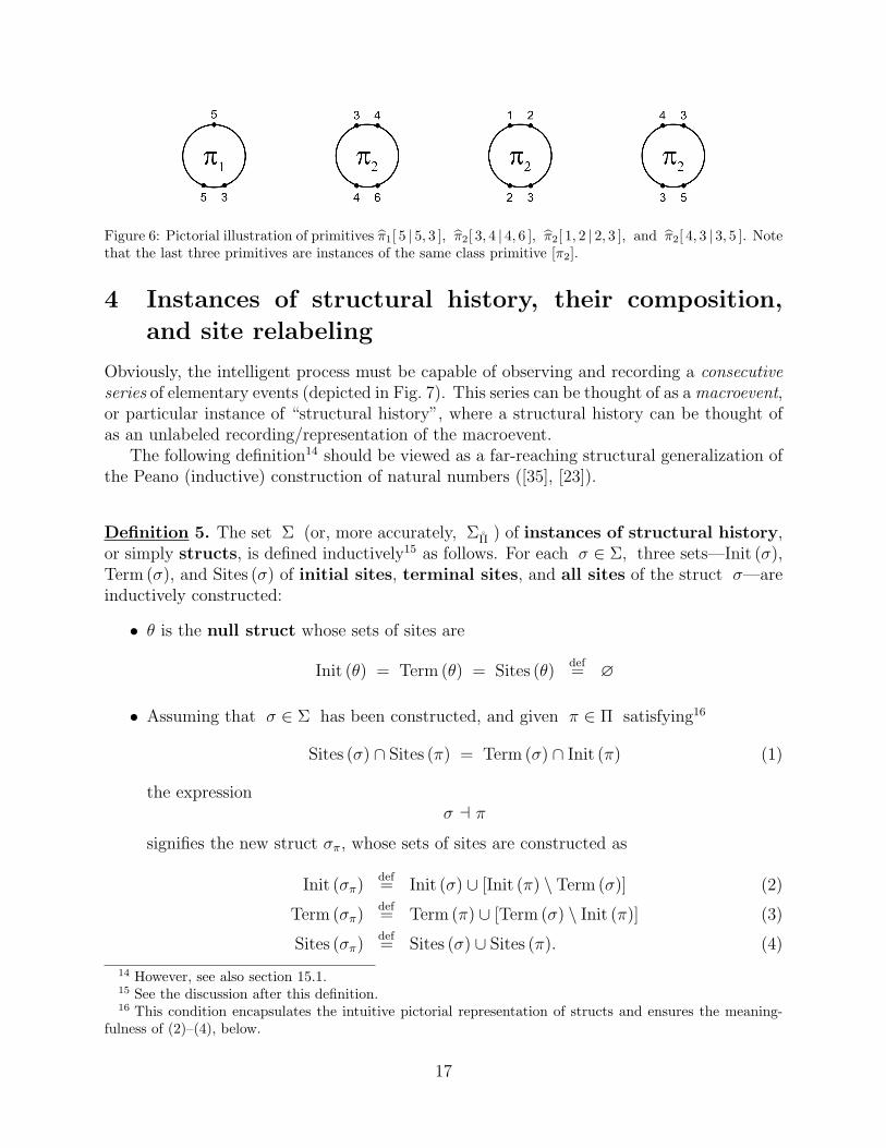
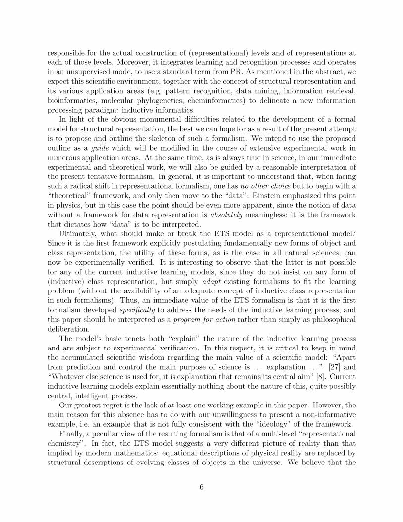
Figure 6: Pictorial illustration of primitives π̂1[ 5 | 5, 3 ], π̂2[ 3, 4 | 4, 6 ], π̂2[ 1, 2 | 2, 3 ], and π̂2[ 4, 3 | 3, 5 ]. Notethat the last three primitives are instances of the same class primitive [π2].

4 Instances of structural history, their composition,

and site relabeling

Obviously, the intelligent process must be capable of observing and recording a consecutiveseries of elementary events (depicted in Fig. 7). This series can be thought of as a macroevent,or particular instance of “structural history”, where a structural history can be thought ofas an unlabeled recording/representation of the macroevent.

The following definition14 should be viewed as a far-reaching structural generalization ofthe Peano (inductive) construction of natural numbers ([35], [23]).

Definition 5. The set Σ (or, more accurately, ΣΠ̊ ) of instances of structural history,or simply structs, is defined inductively15 as follows. For each σ ∈ Σ, three sets—Init (σ),Term (σ), and Sites (σ) of initial sites, terminal sites, and all sites of the struct σ—areinductively constructed:

• θ is the null struct whose sets of sites are

Init (θ) = Term (θ) = Sites (θ)def= ∅

• Assuming that σ ∈ Σ has been constructed, and given π ∈ Π satisfying16

Sites (σ) ∩ Sites (π) = Term (σ) ∩ Init (π) (1)

the expressionσ a π

signifies the new struct σπ, whose sets of sites are constructed as

Init (σπ)def= Init (σ) ∪ [Init (π) \ Term (σ)] (2)

Term (σπ)def= Term (π) ∪ [Term (σ) \ Init (π)] (3)

Sites (σπ)def= Sites (σ) ∪ Sites (π). (4)

14 However, see also section 15.1.15 See the discussion after this definition.16 This condition encapsulates the intuitive pictorial representation of structs and ensures the meaning-

fulness of (2)–(4), below.

17

We call σπ the continuation of struct σ by primitive π, where continuation is depictedand could be thought of as an attachment of the identical sites in Term (σ) and Init (π),explicated below. The operation a is called the continue operation. We specify structσ by the following expression encapsulating its construction process

σ = [π1 a π2 a · · · a πt]

(see Fig. 7). The order relationship between the indices in the last expression correspondsto the constructive order of the relevant continue operations rather than serving as a uniqueprimitive identifier (πi may coincide with πj). We assume that this expression is validfor t = 0 and, in this case, denotes θ. For the above construction of σ a π, we also usethe following terminology: primitive π is attached to primitive πi if, when actuallyconstructing σ a π, at least one initial site π(k) of π was attached to one terminal siteπi(l) of πi. I

Figure 7: Two structs, where the set of original primitives includes π̊1, π̊2, π̊3, π̊4, π̊5. The vertical order ofprimitives corresponds to the constructive (temporal) order of the relevant continue operations.

The proof of the next lemma follows directly from the above definitions.

Lemma 1. Any struct σ, where

σ = [π1 a π2 a · · · a πt],

can also be expressed as

σ = [̊πi1 {f1 } a π̊i2 {f2 } a · · · a π̊it {ft }],

where π̊ij ∈ Πij and fj is an original primitive site relabeling. �

It is important to note that, formally, we view the set Σ not as a derivative of the setof natural numbers, but rather as its precursor. In particular, we view the set of natural

18

numbers as a special case of Σ, where Π̊ consists of a single primitive of very simplestructure17: π̊[ a | a ] (see Fig. 8). Consequently, to achieve a reasonable degree of rigor, weshould rely on the appropriate generalization of the Peano axioms (for natural numbers [28]),including the generalization of the induction axiom (see below). In this paper, however, toretain both rigor and accessibility, we adopt instead the following inductive scheme.

Figure 8: Left: the (single) primitive involved in the ETS representation of natural numbers. Right: structsrepresenting the natural numbers 1, 2, and 3.

By an inductive definition, or specification, of process P (σ) 18 that constructs a structσ ∈ Σ, we mean the following definition, or specification, scheme:

• construct P (θ)

• assume that P (α) has been constructed and that σ = α a π, then construct P (σ).

The above construction relies on the following axiom.

Induction axiom for structs. If Σ′ is a subset of Σ satisfying the following conditions

• θ ∈ Σ′

• ∀σ, σ′ ∈ Σ such that σ′ = σ a π for some π ∈ Π

σ ∈ Σ′ ⇒ σ′ ∈ Σ′

then Σ′ = Σ. I

The next definition introduces two useful kinds of substructs of a given struct σ.

Definition 6. For a given struct σ,

σ = [π1 a π2 a · · · a πt],

17 The set of site labels SL could be chosen to be of cardinality one (abstract natural numbers) or ofgreater cardinality (“concrete” natural numbers, i.e. counting with sticks, stones, etc.).

18 See section 2.

19

and its primitive πk, primitive πj, is a successor of πk (in σ ) if there is a subsequenceof indices i1, i2, . . . , ir, where k = i1 < i2 < · · · < ir = j, such that

πip+1 is attached to πip 1 ≤ p < r.

We also define every primitive to be a successor of itself.For the above struct σ and a subsequence of its primitives 〈πj1 , πj2 , . . . , πjm〉 such that

no primitive is a successor of any other primitive from the set, the minimal struct

σ(πj1 , πj2 , . . . , πjm)def={

[πk1 a · · · a πkn ], 1 ≤ k1 < · · · < kn ≤ t | ∀ πjiall of its successors are in this struct

}is called a successor substruct of σ.

If a successor substruct of σ contains the last primitive of σ, πt, then we call such asubstruct a latest substruct of σ (see Fig. 9). I

Figure 9: Pictorial illustration of a latest substruct of σ.

20

Lemma 2. For a given struct σ and two successor substructs σ(πi1 , πi2 , . . . , πil),σ(πj1 , πj2 , . . . , πjm),

σ(πi1 , πi2 , . . . , πil) = σ(πj1 , πj2 , . . . , πjm) ⇔ {πi1 , πi2 , . . . , πil} = {πj1 , πj2 , . . . , πjm}.

�

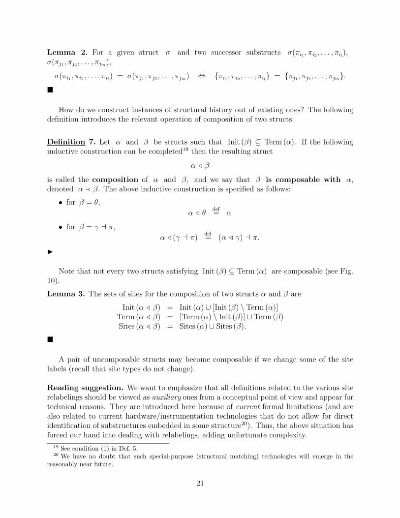
How do we construct instances of structural history out of existing ones? The followingdefinition introduces the relevant operation of composition of two structs.

Definition 7. Let α and β be structs such that Init (β) ⊆ Term (α). If the followinginductive construction can be completed19 then the resulting struct

α / β

is called the composition of α and β, and we say that β is composable with α,denoted α � β. The above inductive construction is specified as follows:

• for β = θ,

α / θdef= α

• for β = γ a π,

α / (γ a π)def= (α / γ) a π.

I

Note that not every two structs satisfying Init (β) ⊆ Term (α) are composable (see Fig.10).

Lemma 3. The sets of sites for the composition of two structs α and β are

Init (α / β) = Init (α) ∪ [Init (β) \ Term (α)]Term (α / β) = [Term (α) \ Init (β)] ∪ Term (β)Sites (α / β) = Sites (α) ∪ Sites (β).

�

A pair of uncomposable structs may become composable if we change some of the sitelabels (recall that site types do not change).

Reading suggestion. We want to emphasize that all definitions related to the various siterelabelings should be viewed as auxiliary ones from a conceptual point of view and appear fortechnical reasons. They are introduced here because of current formal limitations (and arealso related to current hardware/instrumentation technologies that do not allow for directidentification of substructures embedded in some structure20). Thus, the above situation hasforced our hand into dealing with relabelings, adding unfortunate complexity.

19 See condition (1) in Def. 5.20 We have no doubt that such special-purpose (structural matching) technologies will emerge in the

reasonably near future.

21

Figure 10: Two structs (α and β) and their composition (α / β). Note that β / α is not a legal compo-sition.

Definition 8. For a struct σ = [π1 a π2 a · · · a πt], a site relabeling g,

g : Sites (σ) → SL,

is called a site relabeling of struct σ. Moreover, the struct σ{g }, defined as

σ{g }def=

[π1{g|Sites (π1) } a π2{g|Sites (π2) } a · · · a πt{g|Sites (πt)

}],

is called a site-relabeled struct σ (see Fig. 11). I

Figure 11: Pictorial illustrations of a struct, a site relabeling mapping, and the corresponding relabeledstruct.

It is not difficult to see that the following properties hold.

1. For a struct σ and two site relabelings f : Sites (σ) → SL, g : Sites (σ{f }) → SL,we have

(σ{f }){g } = σ{g◦f }.

22

2. If σ′ = σ{f }, then there exists site relabeling f ′ : Sites (σ′) → SL such that σ′ {f ′ } =σ.

3. If α � β and f : Sites (α / β) → SL, fα = f∣∣Sites (α)

, fβ = f∣∣Sites (β)

are site

relabelings, then α{fα } � β{fβ } and

α{fα } / β{fβ } = (α / β){f }.

5 Extructs

In this section we introduce the concept of “extruct”, which may be informally thought ofas a particular fragment of recent history (which must include the latest event). When thecentral concept of “transformation” is introduced in the next section, an extruct will specifythe “context” of a transformation, i.e. a fragment of a struct which identifies the place wherea transformation may originate, while a struct will specify the “body” of a transformation.

We note the tentative nature of the extruct concept: it may change as our understandingof the intelligent process (Part III) evolves.

The next, auxiliary, definition introduces a (partial) encapsulation of a given struct by agraph (see Fig. 12).

Definition 9. The attachment graph for struct σ = [π1 a π2 a · · · a πt] is defined asthe following directed graph:

Gσ = 〈Vσ, Eσ〉,

whereVσ = {v1, v2, · · · , vt}

vi corresponds to πi

and

〈vi, vj〉 ∈ Eσ if, in the inductive construction of σ, πj was attached to πi.

I

When no confusions arises, the subscript σ for the attachment graph will be dropped.Note that multiple attachments between two primitives are recorded as a single edge in theattachment graph (see Fig. 12).

The next (also auxiliary) definition introduces several concepts useful for defining one ofthe main concepts, that of extruct.

Definition 10. An interfaced struct is a pair 〈σ, Iface 〉, where σ is a struct

σ = [π1 a π2 a · · · a πt]

23

Figure 12: Pictorial illustrations of a struct and the corresponding attachment graph.

and Iface is a subset of Term (σ) called the set of interface sites. For each primitiveπi in the above σ, 1 ≤ i ≤ t, a constituent of 〈σ, Iface 〉 is the following 4-tuple

eiσ

def= 〈πi, DISi, DTSi, ISi〉,

where

• DISi is the set of detached initial sites, DISi ⊆ Init (πi), consisting of those initialsites that are not attached to any other primitive;

• DTSi is the set of detached terminal sites, DTSi ⊆ Term (πi) \ Iface , consistingof those terminal sites that are not attached to any other primitive;

• ISi is the set of interfaced sites, ISi ⊆ Term (πi)∩Iface , consisting of those terminalsites that are not attached to any other primitive.

I

24

For example, for interfaced struct⟨σ, {1, 5}

⟩, where σ is depicted in Fig. 12,

e1σ =

⟨π1, {1}, ∅, ∅

⟩,

e2σ =

⟨π2, {2}, ∅, ∅

⟩,

e3σ =

⟨π3, ∅, {7}, ∅

⟩,

e4σ =

⟨π4, ∅, ∅, ∅

⟩,

e5σ =

⟨π5, ∅, ∅, {1}

⟩,

e6σ =

⟨π6, ∅, ∅, ∅

⟩,

e7σ =

⟨π7, ∅, ∅, {5}

⟩.

The following definition specifies a construction procedure which outputs a σ-extruct,which is, in fact, a particular instance of an extruct (defined immediately after this defi-nition). The procedural nature of this definition, as opposed to the previous ones, shouldbe viewed in light of the “needs” of the intelligent process presented in Part III, which willbe actively searching for an occurrence of such an instance in some struct. The procedureconsists of the repeated excision of some constituents of a given interfaced struct, togetherwith the corresponding updates of the remaining constituents.

Definition 11. For an interfaced struct 〈σ, Iface 〉,

σ = [π1 a π2 a · · · a πt],

we perform the following construction procedure. This procedure, called the σ-relatedextruct construction procedure, outputs a σ-related extruct, or simply σ-extruct.The procedure involves zero or more updates of a tuple (see the next paragraph) Ek,k = 0, 1, 2, . . . , final, whose elements are the current constituents of 〈σ, Iface 〉 and outputsa triple 〈σ, Iface , E〉, where E = Efinal.

First, the procedure constructs the attachment graph G0 for σ, then initializes the(current) tuple El, i.e. l = 0, as follows:

E0 def= 〈e1

σ, e2σ, · · · , et

σ〉.

In what follows, we use the same notation eiσ to denote the corresponding current (updated)

4-tuple, and the same is true for its components.Next, ej

σ is allowed 21 to be excised from the current tuple El if its current ISj = ∅.This is accomplished by removing ej

σ from the current tuple, updating the attachment graphGl

22, and, for each non-excised emσ ,

• if πm was attached to πj, updating DISm as follows: the new DISm is the currentDISm plus the sites by which πm was attached to πj in σ,

• if πj was attached to πm, updating DTSm in a similar manner.

21 “Allowed” implies a possibility that, in practice, depends on the chosen strategy.22 The update is accomplished by removing the corresponding vertex and incident edges.

25

The σ-extruct construction procedure is allowed to halt (with the final tuple E, E =Efinal, and the corresponding final attachment graph G, G = Gfinal), if each connectedcomponent G′ of G has the following property:⋃

vi∈VG′

ISi 6= ∅.

Thus, the above σ-extruct is the resulting triple 〈σ, Iface , E〉, denoted εσ,

εσdef= 〈σ, Iface , E〉,

where set Iface is called the set of interface sites of εσ. Obviously, if Iface = ∅, thenthe resulting σ-extruct

εσ = 〈σ, ∅, ∅〉is called the null σ-extruct. The set of all σ-extructs for an interfaced struct 〈σ, Iface 〉 isdenoted E〈σ,Iface 〉. The set of all σ-extructs for all interfaced structs is denoted E . I

Figure 13 illustrates three possible outputs of the above construction procedure for σfrom Fig. 12.

Figure 13: Pictorial illustration of some σ-extructs for the interfaced struct 〈σ, Iface 〉, where σ is shownin Fig. 12. (Heavy lines identify interface sites, crosses identify detached initial/terminal sites.)

Remark 4. Note that the above σ-extruct construction procedure may be specified in greaterdetail, but such a specification is application-dependent.23

23 See also Remark 5 in Section 6.

26

The central concept of this section, introduced next, is a generalization of the σ-relatedextruct obtained by removing the dependence on struct σ, which is one of the input pa-rameters of the corresponding construction procedure in Def. 11.

Definition 12. An extruct ε is defined as an equivalence class for the following equivalencerelation ∼ on the set E . Let

εσ1 = 〈σ1, Iface 1, E1〉 and εσ2 = 〈σ2, Iface 2, E2〉,

thenεσ1 ∼ εσ2 ⇐⇒ Iface 1 = Iface 2 and E1 = E2.

We also use the following notation

εdef= 〈Iface , E〉,

where

Ifacedef= Iface 1,

Edef= E1.

In this context, the set Iface is called the set of interface sites of extruct ε, and theset

Sites (ε)def=

⋃Sites (πi),

where each πi corresponds to eiσ in tuple E, is called the set of all sites of extruct ε.

I

When pictorially illustrating an extruct, we simply use the pictorial illustration of acorresponding σ-extruct.

We now introduce the concept of relabeling for an extruct.

Definition 13. For an extruct ε, a site relabeling g,

g : Sites (ε) → SL,

is called a site relabeling of extruct ε. Moreover, the extruct

ε{g }def= 〈g(Iface ), E{g }〉,

where E{g } is obtained from E by replacing eiσ = 〈πi, DISi, DTSi, ISi〉 (for an appropriate

σ ) witheiσ {g } = 〈πi{g|Sites (πi)

}, g(DISi), g(DTSi), g(ISi)〉,

is called a site-relabeled extruct ε. I

27

6 Transformations and supertransformations

This section might be viewed as the culmination of Part II: in it, we introduce almost allcentral concepts of the proposed framework.

The following definition introduces the first of the three most fundamental concepts ofthe ETS framework, that of “transformation”, which can be thought of as a representationalmodule. A transformation embodies a formative dependence between its two constituentsubmodules: an extruct and the struct that is attached to it (see Fig. 14).

Definition 14. A transformation, or simply transform, is a pair

τ = 〈ε, β〉

where extruct ε = 〈Iface , E〉 and struct β satisfy

Iface = Init (β) = Sites (ε) ∩ Sites (β).

We call ε the context of transform τ , denoted cntx(τ), and β the body of transformτ , denoted body(τ). The set of all sites of transform τ is defined as

Sites (τ)def= Sites (ε) ∪ Sites (β).

The set of all transforms is denoted T . I

Remark 5. The current asymmetry between the concepts of context and body is related tothe fact that the context of a transform has to be “detected” within a given struct, while thetransform’s body is “grown” from the identified context. Context detection is realized viathe σ-related extruct construction procedure (Def. 11). The nature of the process involvedin the growth of the body is sketched in Part III (however, see section 15).

From an applied point of view, it is useful to think of a struct as being “formed”, roughlyspeaking, by a series of transformations, since, in reality, every struct stands for an “object”from some class of objects (see also Defs. 18, 29).

As always, we now need to be able to relabel a transform’s sites.

Definition 15. For a transform τ = 〈ε, β〉, a site relabeling h,

h : Sites (τ) → SL,

is called a site relabeling of transform τ . Moreover, the transform

τ {h}def= 〈ε{h|Sites (ε) }, β{h|Sites (β) }〉,

is called a site-relabeled transform τ . I

28

Figure 14: An example of a transform whose context is an extruct induced by the last σ-extruct in Fig.13. The right hand side depicts the “assembled” transform corresponding to a more appropriate interpreta-tion/understanding of the transform.

We are now ready to introduce a generalization of the transformation concept, that ofsupertransformation, which is achieved by uniting several related transformations (see Fig.15). Although at this moment the role of supertransform is not clarified, we will do so in thenext section, at which point its meaning will also become clearer. Unfortunately, we mustadmit that the following definition of this concept—but not the concept itself—is a transientone (see also the Important remark on p. 36).

Definition 16. A supertransformation, or simply supertransform, is a pair

τdef= 〈E, B〉,

whereE = {ε1, ε2, · · · , εp} εi = 〈Iface i, Ei〉,

B = {β1, β2, · · · , βq},

if the following conditions hold

∀ i, j, kInit (βi) = Init (βj) = Iface k = Sites (εk) ∩ Sites (βi)

Term (βi) = Term (βj) .

The constituent transform set for a supertransform τ is defined as the set of alltransforms specified by the elements of the Cartesian product E ×B.

29

It is convenient for us to blur the distinction between the pair 〈E, B〉 and the productE ×B, and to refer to both of them as the supertransform τ . Thus the following notationwill be used: τ = 〈ε, β〉, τ ∈ τ .

The set of all sites of supertransform τ is defined as

Sites (τ )def=

⋃τ∈τ

Sites (τ).

The set of all supertransforms is denoted T . I

It is easy to see that the concept of a “constituent transform” is meaningful, i.e. theconditions of Def. 14 are satisfied. Moreover, in the terminology of Def. 16, all constituenttransforms share interface sites.

A useful visualization aid for a supertransform τ is the rectilinear table of its constituenttransforms, as shown in Fig. 15.

It is useful to note that there are supertransforms with null contexts: all of its contextsare null, and all of its bodies have no initial sites, i.e. the table in Fig. 15 collapses to a singlerow of bodies.

Again, we need to be able to relabel supertransforms.

Definition 17. For a supertransform τ = 〈E, B〉 (= E ×B), a site relabeling h

h : Sites (τ ) → SL,

is called a site relabeling of supertransform τ . Moreover, the supertransform

τ {h}def= {τ {h|Sites (τ) } | τ ∈ τ}

is called a site-relabeled supertransform τ . I

The following definition is the second of the three most fundamental concepts of the ETSframework; it is a simple/natural generalization of the supertransform concept (see Fig. 16).

Definition 18. A class supertransform is defined as an equivalence class for the followingequivalence relation ≈ on the set T of all supertransforms. Let τ1, τ2 be supertransforms,then

τ1 ≈ τ2 ⇐⇒ τ2 = τ1{g }

for some supertransform site relabeling mapping g. The notation [τ ] is used to denote aclass supertransform containing τ and is called the class induced by τ . I

It is useful to think of a class supertransform as a “structural” description of a class ofobjects that allows for context- and body-related noise variations, including some transforma-tions that only account for noise (see also Def. 29 where further generalization is introduced).We also need a particular “canonical” supertransform standing for the class supertransform.

30

Figure 15: Pictorial illustration of a supertransform. Note that all contexts have the same interface sitesand all bodies have the same initial and terminal sites.

Lemma 4. For any class supertransform [τ ] there exists an efficient, implementation-dependent algorithm that uniquely constructs a particular supertransform τ̊ , τ̊ ∈ [τ ].�

The lemma leads naturally to the next definition (see also Remark 2, p. 16).

Definition 19. The unique supertransform τ̊ constructed in the above lemma is called thecanonical supertransform for class supertransform [τ ]. I

The existence of canonical supertransforms simplifies the algorithmic processing and stor-age of class supertransforms and also facilitates a transition between two adjacent levels ofrepresentation (see the next section). Further, any supertransform υ ∈ [τ ] can now bespecified simply by providing a site relabeling h such that υ = τ̊ {h}.

31

Figure 16: Pictorial illustration of a class supertransform induced by the supertransform depicted in Fig.15. Each letter is the name of a variable that is allowed to vary over numeric labels of the same type, asexplained in the caption of Fig. 5 (site types are not shown).

How does one expand a class supertransform on the basis of a given transform υ whosebody is present in that class supertransform? For the set of bodies in the canonical super-transform (from the class supertransform) that are relabelings of the body of υ, we add thesame number of contexts, each of which is an appropriately relabeled context of υ.

Definition 20. For a given transform υ,

υ = 〈ζ, γ〉,

and class supertransform [τ ], with canonical supertransform τ̊ = 〈E, B〉, let set G bethe set of all the relabelings g of body γ such that γ{g } is in B:

G def=

{g : Sites (γ) → SL | γ{g } ∈ B

}.

32

Moreover, let set H be a set of relabelings of υ that are extensions of g’s and such thatfor each g ∈ G there exists unique h ∈ H satisfying

h|Sites (γ) = g

Sites (τ̊ ) ∩ h(Sites (ζ) \ Sites (γ)

)= ∅.

If G 6= ∅, let

E expdef= E ∪

{ζ {h|Sites (ζ) } | h ∈ H

}.

The context expansion of class supertransform [τ ] w.r.t. transform υ, denoted[τ , cntx(υ)], is defined as the class supertransform induced by the supertransform

τcntx(υ)def= 〈E exp, B〉.

The concept of the body expansion of class supertransform [τ ] w.r.t. transformυ, denoted [τ , body(υ)], is defined similarly by exchanging the roles of ζ and γ in theabove. I

7 Transition to a new level of representation

What necessitates the transition (within an information processing system) to a new level ofrepresentation is the need to deal more effectively with the complexity of event representa-tion. In AI this was often called “chunking” [37]. Within the ETS model, such a transitionconsists of the construction of a new (next-level) set of primitives, which can then be usedconstructively in the usual manner (including construction of structs, extructs, transforms,etc.).

How does one encapsulate the information contained in a class supertransform in the formof a new primitive in order to legitimately reduce the complexity of an event representation?As a transitory working version, we propose the following postulate to deal with this question.This postulate is based on a considerable oversimplification related to the fact that we havechosen to almost completely ignore the structure of the contexts and the bodies of thesupertransform24.

Level ascension postulate. The class of (context-sensitive) macroevents correspondingto a canonical supertransform may be adequately represented at the next level by a new(original) primitive obtained by completely shrinking that supertransform’s contexts and bydropping the internal structure of the supertransform’s bodies in the manner described inDef. 21. I

Notational convention 1. From this section onwards, next-level notations will be denotedwith the addition of a superscript prime to the corresponding present-level notation.

24 However, see section 15.2.

33

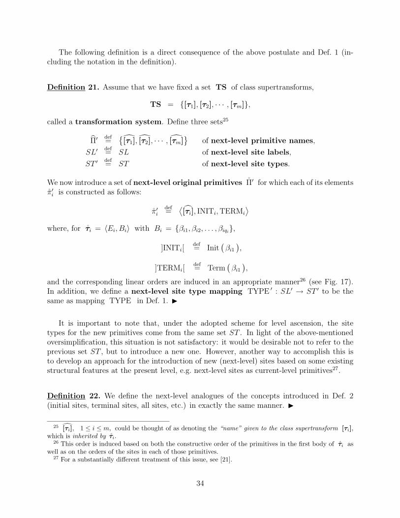
The following definition is a direct consequence of the above postulate and Def. 1 (in-cluding the notation in the definition).

Definition 21. Assume that we have fixed a set TS of class supertransforms,

TS = {[τ1], [τ2], · · · , [τm]},

called a transformation system. Define three sets25

Π̂′ def=

{[̂τ1], [̂τ2], · · · , [̂τm]

}of next-level primitive names,

SL′ def= SL of next-level site labels,

ST ′ def= ST of next-level site types.

We now introduce a set of next-level original primitives Π̊′ for which each of its elementsπ̊′

i is constructed as follows:

π̊′i

def=

⟨[̂τi], INITi, TERMi

⟩where, for τ̊i = 〈Ei, Bi〉 with Bi = {βi1, βi2, . . . , βiqi

},

]INITi[def= Init

(βi1

),

]TERMi[def= Term

(βi1

),

and the corresponding linear orders are induced in an appropriate manner26 (see Fig. 17).In addition, we define a next-level site type mapping TYPE ′ : SL′ → ST ′ to be thesame as mapping TYPE in Def. 1. I

It is important to note that, under the adopted scheme for level ascension, the sitetypes for the new primitives come from the same set ST . In light of the above-mentionedoversimplification, this situation is not satisfactory: it would be desirable not to refer to theprevious set ST , but to introduce a new one. However, another way to accomplish this isto develop an approach for the introduction of new (next-level) sites based on some existingstructural features at the present level, e.g. next-level sites as current-level primitives27.

Definition 22. We define the next-level analogues of the concepts introduced in Def. 2(initial sites, terminal sites, all sites, etc.) in exactly the same manner. I

25 [̂τi], 1 ≤ i ≤ m, could be thought of as denoting the “name” given to the class supertransform [τi],which is inherited by τ̊i.

26 This order is induced based on both the constructive order of the primitives in the first body of τ̊i aswell as on the orders of the sites in each of those primitives.

27 For a substantially different treatment of this issue, see [21].

34

Figure 17: A canonical supertransform (from a class supertransform taken from a transformation system)and the corresponding next-level original primitive. Note that, as previously mentioned in the caption ofFig. 4, the symbol ̂ in the depiction of the (next-level) original primitive is dropped.

Definition 23. We define the next-level analogues of the concepts introduced in Def. 4(original primitive site relabeling, primitives, etc.) in exactly the same manner. I

We are now ready to state an improved version of the above correspondence postulate.

Refined level ascension postulate. The ascension to the next level is based on thefollowing basic correspondence28

τ̊i → π̊′i (5)

∀ τ , τ = τ̊i{h} τ → π′ = π̊′i{h|Sites (π̊′

i) } (6)

where the notation in (5) comes from Defs. 19, 21 and the notation in (6) comes from Defs.19, 2329.

All other correspondences between adjacent levels are implications of the above corre-spondence. For example, a next-level struct corresponds to a previous-level superstructcomposed of structs (bodies), where each body is that of one of the transforms from thecorresponding supertransform. I

28 The arrow → denotes ascension to the next level. See also Remark 2 in Sec. 3.29 See also the paragraph following Def. 19.

35

Important remark. In view of the above correspondence (5), we note that the restrictionsimposed on a supertransform in Def. 16 are not quite sufficient: it is intuitively clear that thesupertransform must satisfy some additional constraints ensuring the closer interrelationshipof its constituent transform’s bodies (see Fig. 18).

Figure 18: Three “consistent”, but otherwise quite unrelated bodies.

Finally, we can encapsulate the entire developed mathematical structure as a single entityin the following definition.

Definition 24. A (single-level) inductive structure is a pair

〈Π̊,TS〉,

where Π̊ is a set of original primitives and TS is a transformation system. However, as wasmentioned above, the latter pair also signifies all relevant concepts, such as structs, extructs,etc.

A multi-level inductive structure (with l levels) MIS is an l-tuple

MIS def=

⟨〈Π̊,TS〉, 〈Π̊′,TS′〉, · · · , 〈Π̊(l−1),TS(l−1)〉

⟩,

where TS(l−1) = ∅, TS(k) is the transformation system for the set of original primitivesΠ̊(k), and every consecutive pair of inductive structures satisfies the (refined) level ascensionpostulate (see Figs. 19, 20). For the k-th level inductive structure

⟨Π̊(k),TS(k)

⟩in MIS,

we use the notation

MIS(k)def= 〈Π̊(k),TS(k)〉 k = 0, 1 · · · , l − 1

τ (k) → π(k+1) k = 0, 1 · · · , l − 2.

I

36

Figure 19: Schematic representation of a multi-level inductive structure with l levels.

Notational convention 2. For a transform τ from τ , where τ ∈ [τ ] ∈ TS, we use thefollowing simplified notation τ ∈ τ ∈ TS. Similarly, for the latter supertransform τ , wewrite τ ∈ TS.

37

Figure 20: Pyramid view (partial) of a k-th level class supertransform: the pyramid should be thought of asbeing formed by the subordinate class supertransforms.

38

Part III

The intelligent process:a provisional sketch

Our understanding of the world is built up of innumerable layers. Eachlayer is worth exploring, as long as we do not forget that it is one of many.Knowing all there is to know about one layer—a most unlikely event—wouldnot teach us much about the rest.

E. Chargaff, Heraclitean Fire: Sketches from a Life before Nature, 1978

Part III is built around the intelligent process, which is outlined in sections 10–13. Sec-tions 8, 9 are supporting sections.

Thus, in this part, our focus is on various constructive processes, mainly those relatedto the (temporal) construction of transformations on the basis of the input structs. Suchtranformations either expand the existing class supertransforms or initiate new ones. Thisexplains the change of emphasis in this part.

8 Applicability and appearance of transformations

In this section, we collected two important concepts related to “structural matching” thatare also used in the description of the intelligent process.

The following definition encapsulates the idea of an extruct that has just appeared in agiven struct, i.e. the latest primitive in a given struct (from the viewpoint of the temporalconstruction of the struct) has just enabled the identification of some relabeling of the extruct(see Fig. 21).

Definition 25. For an extruct ε and a struct σ,

σ = [π1 a π2 a · · · a πt],

we say that extruct ε has just appeared in struct σ if there exists σ-extruct εσ =〈σ, Iface , E〉, where εσ ∈ ε, such that

πt is present in the last 4-tuple of E

(see Def. 10). We denote this relation between extruct and struct as follows

ε l σ.

I

39

Figure 21: Pictorial illustration of an extruct ε that has just appeared in struct σ: ε{g } l σ.

The next concept encapsulates the idea of the “applicability” of a supertransform to astruct.

Definition 26. If, for some supertransform τ = 〈E, B〉 and struct σ, there exists contextε ∈ E and extruct site relabeling g : Sites (ε) → SL such that

ε{g } l σ,

then we say that τ is currently applicable to struct σ.For a given multi-level inductive structure MIS and a struct σ(k) from MIS(k) =⟨

Π̊(k),TS(k)⟩, 0 ≤ k ≤ l − 1, we define the set of all k-th level canonical supertrans-

forms that are currently applicable to struct σ(k) as

T appl(σ(k))

def= {τ̊ ∈ [τ ] ∈ TS(k) | τ̊ is currently applicable to struct σ(k)}

(see Notational Convention 2 after Def. 24). I

In a manner similar to the appearance of an extruct, we now introduce the appearanceof a transformation (w.r.t. some struct).

Definition 27. For a transform τ = 〈ε, β〉 and a struct σ, we say that a transform τhas just appeared in struct σ if there exist structs α, γ such that

σ = γ / α, β is a latest substruct of α (Def. 6), ε l γ

(see Fig. 22). We denote this relation between transform and struct as follows

τ l σ.

I

40

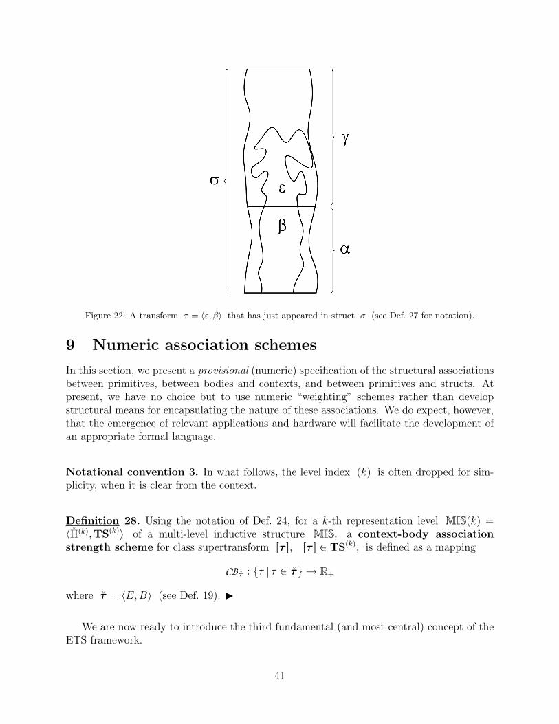
Figure 22: A transform τ = 〈ε, β〉 that has just appeared in struct σ (see Def. 27 for notation).

9 Numeric association schemes

In this section, we present a provisional (numeric) specification of the structural associationsbetween primitives, between bodies and contexts, and between primitives and structs. Atpresent, we have no choice but to use numeric “weighting” schemes rather than developstructural means for encapsulating the nature of these associations. We do expect, however,that the emergence of relevant applications and hardware will facilitate the development ofan appropriate formal language.

Notational convention 3. In what follows, the level index (k) is often dropped for sim-plicity, when it is clear from the context.

Definition 28. Using the notation of Def. 24, for a k-th representation level MIS(k) =〈Π̊(k),TS(k)〉 of a multi-level inductive structure MIS, a context-body associationstrength scheme for class supertransform [τ ], [τ ] ∈ TS(k), is defined as a mapping

CB τ̊ : {τ | τ ∈ τ̊} → R+

where τ̊ = 〈E, B〉 (see Def. 19). I

We are now ready to introduce the third fundamental (and most central) concept of theETS framework.

41

Definition 29. For a k-th representation level, an (inductive) class representation isdefined as the following pair

CLASS [τ ]def=

⟨[τ ] , CB τ̊

⟩,

where class supertransform [τ ] ∈ TS(k) and CB τ̊ is the context-body association strengthscheme for [τ ], also called the class weight scheme. I

In the ETS formalism, the intelligent process relies on class representations to recognize(and also generate) objects from a class. The (scalar valued) strength of evidence for theclass can be derived from the class weight scheme CB τ̊ .

Notational convention 4. To simplify some formulas in the rest of the paper, we usethe notation π̊(i), π̊(j) (see Def. 2) to denote not only the corresponding sites, but thefollowing pairs,

⟨̊π, π̊(i)

⟩, 〈̊π, π̊(j)〉, respectively.

The next definition encapsulates the concept of a (given) weighting scheme specifying thepropensity for sites to be attached, i.e. the weight between two sites of primitives reflects theobserved frequency of their attachment, and thus the projected likelihood of such attach-ments in the future. To do this, we need to introduce the set of admissible site pairs (see Fig.23), which will be used in the rest of the section as the “standard” domain for mappings.

Definition 30. For a k-th representation level MIS(k), with its set of original primitives

Π̊(k) = [̊π(k)1 , π̊

(k)2 , · · · , π̊

(k)nk ], and its site type mapping TYPE (Def. 21), a set LEGAL of

admissible site pairs (site pair attachments) is

LEGALdef=

{⟨̊π

(k)p (i), π̊

(k)q (j)

⟩| TYPE

(̊π

(k)p (i)

)= TYPE

(̊π

(k)q (j)

)}.

A (site-wise primitive) attachment strength scheme or primitive association strengthscheme (PASS) related to the above representation level is a normalized mapping

AS : LEGAL → R+

i.e. ∑LEGAL

AS(

π̊(k)p (i), π̊(k)

q (j))

= 1.

I

A useful notation: J K . If some real-valued mapping A defined on the above set LEGAL

A : LEGAL → R+

is not normalized, then one can easily normalize it to obtain the normalized mapping JAK.

42

Figure 23: Left: two class primitives from Fig. 5. Right: a pictorial encapsulation of the corresponding setLEGAL. Each row and each column corresponds to the indicated site of the corresponding original primitive.

The following definition, based on the above PASS, introduces the concept of the propen-sity of a given primitive to continue a given struct. Moreover, for the rest of the section, recallfrom Def. 4 that if π

(k)1 , π

(k)2 ∈ Π(k), then there exist indices p, q and original primitive site

relabelings f1, f2 such that

π(k)1 = π̊

(k)p {f1 } π

(k)2 = π̊

(k)q {f2 }.

Definition 31. For a fixed representation level (k), let a struct σ be given as

σ = [̊πn1 {f1 } a π̊n2 {f2 } a · · · a π̊nt {ft }]

(see Lemma 1). Given a primitive π (= π̊m {f }), the set LEGAL (σ a π),LEGAL (σ a π) ⊆ LEGAL, is defined as

LEGAL (σ a π)def=

{〈̊πnp(i), π̊m(j)〉 | π̊m {f }(j) is attached to π̊np {fp }(i) in σ a π

}.

43

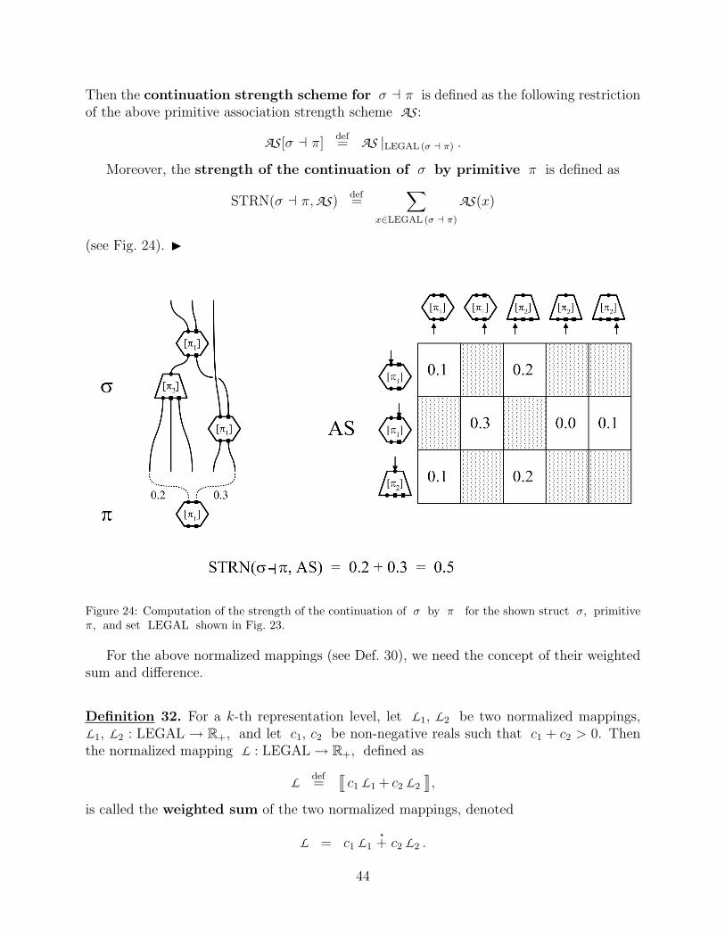
Then the continuation strength scheme for σ a π is defined as the following restrictionof the above primitive association strength scheme AS :

AS [σ a π]def= AS |LEGAL (σ a π) .

Moreover, the strength of the continuation of σ by primitive π is defined as

STRN(σ a π, AS)def=

∑x∈LEGAL (σ a π)

AS(x)

(see Fig. 24). I

Figure 24: Computation of the strength of the continuation of σ by π for the shown struct σ, primitiveπ, and set LEGAL shown in Fig. 23.

For the above normalized mappings (see Def. 30), we need the concept of their weightedsum and difference.

Definition 32. For a k-th representation level, let L1, L2 be two normalized mappings,L1, L2 : LEGAL → R+, and let c1, c2 be non-negative reals such that c1 + c2 > 0. Thenthe normalized mapping L : LEGAL → R+, defined as

L def=

qc1 L1 + c2 L2

y,

is called the weighted sum of the two normalized mappings, denoted

L = c1 L1

�+ c2 L2 .

44

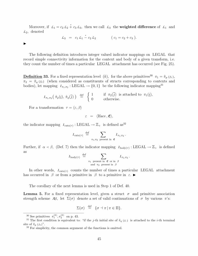
Moreover, if L1 = c2 L2

�+ c3 L3, then we call L3 the weighted difference of L1 and

L2, denoted

L3 = c1 L1

�− c2 L2 ( c1 = c2 + c3 ).

I

The following definition introduces integer valued indicator mappings on LEGAL thatrecord simple connectivity information for the context and body of a given transform, i.e.they count the number of times a particular LEGAL attachment has occurred (see Fig. 25).

Definition 33. For a fixed representation level (k), for the above primitives30 π1 = π̊p {f1 },π2 = π̊q {f2 } (when considered as constituents of structs corresponding to contexts andbodies), let mapping I π1,π2 : LEGAL → {0, 1} be the following indicator mapping31

I π1,π2

(π̊p(i), π̊q(j)

) def=

{1 if π2(j) is attached to π1(i),0 otherwise.

For a transformation τ = 〈ε, β〉

ε = 〈Iface , E〉,

the indicator mapping I cntx(τ) : LEGAL → Z+ is defined as32

I cntx(τ)def=

∑π1,π2 present in E

I π1,π2 .

Further, if α � β, (Def. 7) then the indicator mapping I body(τ) : LEGAL → Z+ is definedas

I body(τ)def=

∑π1 present in E or in β

and π2 present in β

I π1,π2 .

In other words, I cntx(τ) counts the number of times a particular LEGAL attachmenthas occurred in β or from a primitive in β to a primitive in ε. I

The corollary of the next lemma is used in Step 1 of Def. 40.

Lemma 5. For a fixed representation level, given a struct σ and primitive associationstrength scheme AS , let Σ(σ) denote a set of valid continuations of σ by various π’s:

Σ(σ)def= {σ a π |π ∈ Π}.

30 See primitives π(k)1 , π

(k)2 on p. 43.

31 The first condition is equivalent to: “if the j-th initial site of π̊q {f1 } is attached to the i-th terminalsite of π̊p {f2 }”.

32 For simplicity, the common argument of the functions is omitted.

45

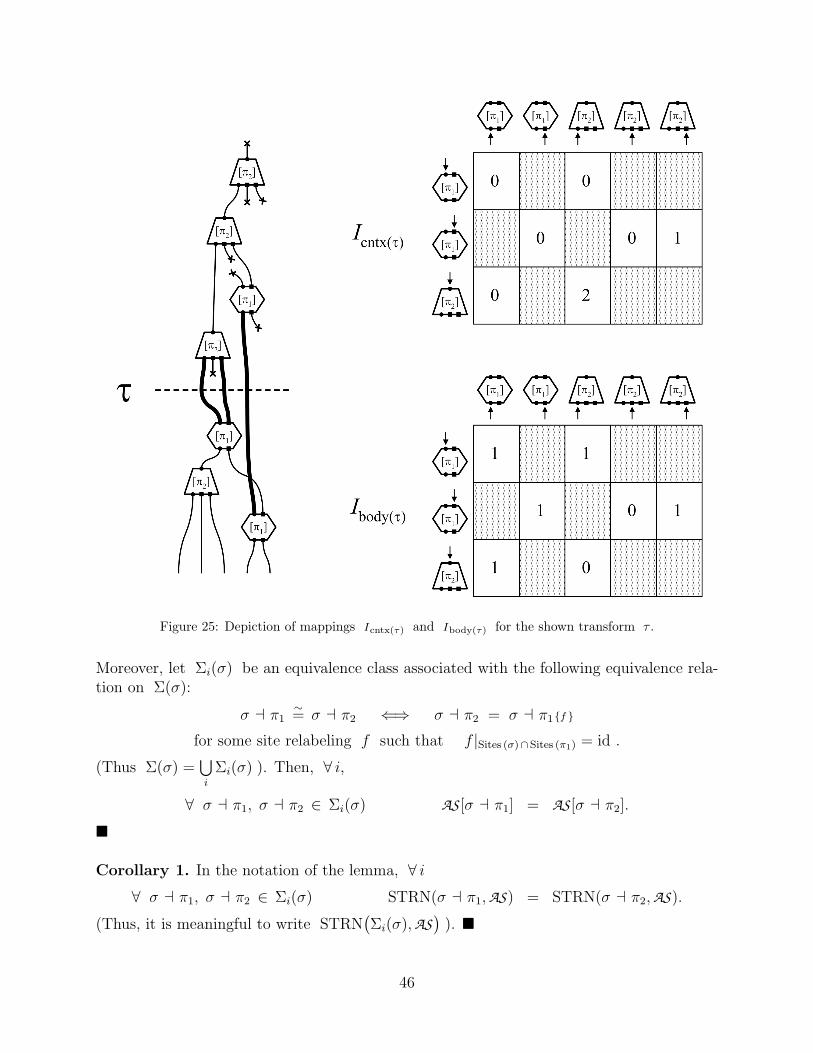
Figure 25: Depiction of mappings I cntx(τ) and I body(τ) for the shown transform τ .

Moreover, let Σi(σ) be an equivalence class associated with the following equivalence rela-tion on Σ(σ):

σ a π1∼= σ a π2 ⇐⇒ σ a π2 = σ a π1{f }

for some site relabeling f such that f |Sites (σ)∩ Sites (π1) = id .

(Thus Σ(σ) =⋃i

Σi(σ) ). Then, ∀ i,

∀ σ a π1, σ a π2 ∈ Σi(σ) AS [σ a π1] = AS [σ a π2].

�

Corollary 1. In the notation of the lemma, ∀ i

∀ σ a π1, σ a π2 ∈ Σi(σ) STRN(σ a π1, AS) = STRN(σ a π2, AS).

(Thus, it is meaningful to write STRN(Σi(σ), AS

)). �

46

10 The intelligent process and its states: introduction

In this section, we initiate the description of a more appropriate, global, view (associatedwith the functioning of the intelligent process) of all the relevant “construction processes”mentioned previously, e.g. struct construction, extruct construction.

In this paper we address only the unsupervised version of the intelligent process, whichcould be modified to handle the supervised case.

Explanatory definition of the intelligent process. An intelligent process P is aprocess which “optimally” captures/represents the development33 of some universe by ex-panding and refining (in a discrete mode) its multi-level inductive structure MIS, includingthe number of its levels. It accomplishes this mainly by the creation and modification (butnever deletion) of relevant class supertransforms at the appropriate levels.

Sections 12 and 13 contain the relevant formal details related to the description of theintelligent process.

Auxiliary notation. To specify the evolution of process P, we call an instantaneousdescription of such a process its (hidden) state, denoted state, and assume that, as-sociated with each such state of process P, is a multi-level inductive structure MISP

state

encapsulating its structural description. Some hidden states are also called observable states,denoted STATE.

The following definition introduces the concept of a k-th level in the state of an intelligentprocess. This results in a multi-level state concept.

Definition 34. For an intelligent process P with its evolving multi-level inductive struc-ture MISP , the k-th level of its (hidden) state is a 3-tuple

state P(k)def=

⟨MISP

state (k), WMPstate (k), AMP

state (k)⟩,

where34:

• MISPstate (k) is the corresponding k-th level (single-level) inductive structure (see Def.

24)

• the k-th level working (structural) memory WMPstate (k) is a pair

WMPstate (k)

def=

⟨σ

(k)state , USED

(k)state

⟩,

where σ(k)state is a struct,

σ(k)state = [π1 a π2 a · · · a πt],

33 More specifcally, we mean an event view of this development, see Sec. 2 and Fig. 3.34 The index P will often be dropped.

47

called the working struct, that records the event history as it is seen from this leveland USED

(k)state is a mapping,

USED(k)state : {1, 2, . . . , t} → {yes, no},

which marks each primitive πi, 1 ≤ i ≤ t, of σ(k)state as “processed” (or “used”) or

not35; note that for σ(k)state = θ, USED

(k)state does not need to be specified

• the k-th level association (schemes) memory AMPstate (k) is a pair

AMPstate (k)

def=

⟨AS (k)

state , {CB state , τ̊ | τ̊ ∈ TS(k)state }

⟩,

where mapping AS (k)state is used by the process to store recently-observed site-wise prim-

itive attachment strengths (Def. 30) and each mapping CB state , τ̊ is used to maintainthe corresponding class weight schemes (Def. 28).

I

Note that the working struct σ(k)state can, in fact, be comprised of several “disjoint” structs

(i.e. those with no site in common). Moreover, from an applied perspective, it is sufficientto deal only with small working structs36.

Remark 6. From a conventional point of view, it is useful to think that the “recognition” ofa supertransform at level k is signified by the attachment of the corresponding (k + 1)-level

primitive to σ(k+1)state . This remark should provide some bridge between conventional PR ideas

and those presented here.

The next concept puts all the levels of a state together, and also clarifies the transitionbetween observable states.

Definition 35. The state of process P is defined as

state Pdef=

⟨state P(0), state P(1), · · · , state P(l − 1)

⟩,

where l is the number of levels in MISPstate .

A state transition in an intelligent process P from some presently observable stateSTATE pres to the next observable state STATE next is comprised of a sequence of hiddenstates:

state pres , state pres+1, · · · , state last ,

where

state presdef= STATE pres , state last

def= STATE next .

I

35 This primitive marking is necessary mainly for the reason that transform bodies are only searched forin the “unprocessed part” of σ

(k)state .

36 This is true in view of the observation that, at each level, only a relatively recent event history needsto be considered.

48

11 Availability of a transformation and fitness of its

parts

As was stated in the explanatory definition of the intelligent process, the intelligent processconstantly expands and refines its multi-level inductive structure. In part, this is accom-plished by either creating a new class supertransform (and, therefore, a new primitive) orby expanding an existing one. To this end, the process will first need to identify relevantcandidate transformations, which are introduced in this section as transforms that have “justbecome available”.

The first definition introduces two numeric measures related to the fitness of each part ofa transform, which will be used for the identification of the candidate transforms introducedin the next (main) definition of the section.

Definition 36. For a k-th representation level in state state P , given two application-

dependent constants d(k)cntx and d

(k)body and a transform τ = 〈ε, β〉, τ ∈ τ ∈ TS

(k)state , the

fitness of the context of τ is

Fitcntx(τ)def= d

(k)cntx −D

(AS (k)

state

�− C

(k)τ ·

qI body(τ)

y,q

I cntx(τ)

y),

where C(k)τ is the (application-dependent) transform fitness coefficient, and the fitness of

the body of τ is

Fitbody(τ)def= d

(k)body −D

(AS (k)

state ,q

I body(τ)

y),

where D is some fixed dissimilarity/distance measure37 on the set of all normalized map-pings whose domain is LEGAL and

qIy

stands for the normalized mapping obtained bynormalizing mapping I (see Def. 30). I

Definition 37. We say that a transformation38 τ (k) = 〈ε, β〉 has just become available(in state P(k) ) of an intelligent process P if

• ( τ has just appeared in σ(k)state )

τ (k) l σ(k)state (Def. 27)

• (each primitive of body(τ) that appears, possibly relabeled, in σ(k)state has not been

used)

for every primitive π(k) in β USED(k)state (j) = no

where j is the index of the primitive in σ(k)state corresponding to the relabeled π(k)

37 E.g. the most popular, Euclidean, distance measure.38 This transformation may not be in any of the class supertransforms from TS(k)

state .

49

• (the next-level primitive induced by τ is attachable to σ(k+1)state )

if, for a supertransform τ̊ (k) = {τ}, formed by the single transform τ , the next-levelcontinuation

σ(k+1)state a π̊(k+1)

where τ̊ (k) → π̊(k+1),

is legal

• ( τ is “fit” with respect to AS (k)state )

Fitcntx(τ) > 0 Fitbody(τ) > 0.

For the process P in state stateP(k), the set Tavail

(stateP(k)

)is defined as the set

of all transforms that have just become available in stateP(k). I

12 Process initiation and state transitions

We now introduce the very first state of the intelligent process.

Definition 38. The initial (observable) state, STATE initial , of an intelligent processP is any valid state of process P (see Def. 35), and possibly even with the following “nullstate”:

STATE initialdef=

⟨〈 MIS initial (0), WM initial (0), AM initial (0) 〉

⟩,

whereMIS initial (0)

def=

⟨Π̊

(0)initial , ∅

⟩WM initial (0)

def=

⟨θ , USED

(0)initial is an empty mapping

⟩AM initial (0)

def=

⟨AS (0)

initial , ∅⟩.

I

We note that the intelligent process never halts, in view of the nature of the transitioninitiation stage (see Step 1 in Def. 40).

Next, we introduce the basic organization of a transition between any two consecutiveobservable states.

Definition 39. We divide an observable state transition from the present observable stateSTATE pres (= state pres ) to the next observable state STATE next (= state last )

39, intotwo stages: the transition initiation stage and the multi-level transition stage. I

39 See Def. 35.

50

The first of the latter two stages is relatively simple and basically consists of choosing aprimitive at level zero in order to continue the level zero working struct. However, beforeproceeding with the definition of the transition initiation stage, we need to briefly mentionthe role of “sensor(s)” in the intelligent process. Without going into detail, we assume theprocess relies on its sensor(s), whose main function is related to the simultaneous updatingof the association strength schemes AS (k) at a number of levels s, where s depends onthe structure of the sensor.

Definition 40. The transition initiation stage is comprised of the following three steps.

Step 1 (parallel update of association memory by sensor(s)). Sensor(s) update associationstrength schemes at several levels by updating the entries associated with sensed data.

Step 2 (primitive selection at level zero). Let

WM pres (0) =⟨σ

(0)pres , USED(0)

pres

⟩,

where

σ(0)pres = [π

(0)1 a π

(0)2 a · · · a π

(0)t ].

The choice of the primitive π(0)pres (= π̊

(0)pres {f }) to be attached to the working struct is

performed by, first, randomly choosing40 Σi(σ(0)pres ) (from the corresponding partition of

Σ(σ(0)pres ) ) with probability proportional to STRN

(Σi(σ

(0)pres ), AS (0)

), and, second, by select-

ing a particular σ(0)pres a π

(0)pres from the chosen Σi(σ

(0)pres ).

Step 3 (advance to the next state by updating working memory at level zero). Define thenext hidden state as

state pres+1def=

⟨state pres+1(0), state pres (1), · · · , state pres (l − 1)

⟩,

in which the only level being updated is level 0

statepres+1(0)def= 〈 MISpres (0), WM pres+1(0), AM pres+1(0) 〉,

where the last two entries are defined as follows:

• (continue the working struct by π(0)pres )

WM pres+1(0)def=

⟨σ

(0)pres a π

(0)pres , USED

(0)pres+1

⟩,

USED(0)pres+1 is an extension of USED(0)

pres with USED(0)pres+1(t + 1) = no

40 For the notation, see Lemma 5 and its corollary in Sec. 9. This complication is an artifact of thenecessity of dealing with a possibly infinite set of relabeled primitives.

51

• (increase association strengths between π(0)pres and the primitives it was just attached

to)

AM pres+1(0)def=

⟨AS (0)

pres+1 , {CB pres , τ̊ | τ̊ ∈ TS(0)pres }

⟩,

AS (0)pres+1 = AS (0)

pres

�+

rAS (0)

pres [σ(0)pres a π

(0)pres ]

z.

I

We are now ready to present the organization of the main stage in the transition betweentwo observable states.

Definition 41. The multi-level transition stage, at each level k (beginning with k = 0),is comprised of the following three consecutive steps41, comprising a k-th level transitionsubstage:

• the learning step (Def. 42)

• the recognition step (Def. 43)

• the facilitation step (Def. 44).

On completion of the k-th level transition substage, check whether the termination flag42

has been raised: if so, then the entire multi-level transition stage is completed, otherwiseproceed to the next level, level (k + 1).

A more detailed depiction of the multi-level transition stage is presented in Fig. 26. Weassume that the multi-level transition stage terminates at some level m, where 0 ≤ m ≤ l−1.I

We note that, at present, the names of the steps express their intended meaning, ratherthan the current, possibly inadequate, implementations of the corresponding steps.

13 The k-th level transition substage

This section is written in an algorithmic style, which is more appropriate, given the natureof the subject matter, and it’s “definitions” are actually algorithmic descriptions of thecorresponding steps. For implementational details, see [10].

We strongly suggest that, during the reading of this section, readers should convincethemselves that, as expected, structural considerations transcend numeric ones in the func-tioning of the intelligent process. Since all definitions in this section refer to the same levelk, we will often omit the level index (k) unless confusion arises. We suggest that it may beuseful to review carefully Fig. 26. Also note the following convention when presenting eachof the following steps: in each case, after updating the start state state step-start , we switchto the notation state step to denote the resulting hidden state.

41 Each of these steps involves a single hidden state transition.42 The termination flag may be implemented as a boolean variable set to “FALSE” at the beginning of

each transition initiation stage (Def. 40).

52

Fig

ure

26:

Not

atio

nalco

nven

tion

for

the

mul

ti-lev

eltr

ansi

tion

stag

e.T

here

cogn

itio

nan

dle

arni

ngst

eps

invo

lve

subs

teps

(not

show

n).

53

13.1 The learning step

This subsection outlines the first (learning) step in the k-th level transition substage, whichinvolves the possible discovery of new or modification of existing class descriptions at thislevel.

Definition 42. For a k-th level transition substage of an intelligent process P, the learn-ing step consists of the following 3 substeps.

Substep 1. Identify the set T(k)avail( state learn-start ) of all transforms that have just become

available in state learn-start (see Def. 37). If T(k)avail( state learn-start ) = ∅ then end the

learning step, i.e. state learn-end = state learn-start .

Substep 2. Choose a transform υ from T(k)avail( state learn-start ) for which Fit

(k)body(υ) is max-

imal (with ties broken based on Fit(k)cntx(υ)).

Substep 3. For the chosen transform υ,

υ = 〈ε, β〉,

• ( υ has been learned previously)

IF υ ∈ τ ∈ TS(k)learn-start , then end the learning step

• (β has been learned previously)

IF, for some43 class supertransform [τ ] ∈ TS(k)learn-start (with canonical supertransform

τ̊ ), [τ , cntx(υ)] is a valid context expansion of [τ ] w.r.t. υ (Def. 20), then updatestate learn-start as follows:

– update AM learn-start (k) by replacing only one of its class weight schemes,i.e. CB learn-start , τ̊ (for the above [τ ] ), with its extension CB learn-start , τ̊1

(corresponding to [τ , cntx(υ)] whose canonical supertransform is τ̊1 )

CB learn-start , τ̊1

(τ) def

=

CB learn-start , τ̊

(τ)

τ ∈ τ̊∑x∈LEGAL

I body(τ)(x) ∃h τ = υ{h}

implementation-dependent otherwise

– replace [τ ] with [τ , cntx(υ)]

• ( ε has been learned previously)

IF, for some class supertransform [τ ] ∈ TS(k)learn-start , [τ , body(υ)] is a valid body

expansion of [τ ] w.r.t. υ, then update state learn-start as follows:

43 Note that there exists at most one such class supertransform [τ ].

54

– update AM learn-start (k) as above, exchanging the roles of the context and body

– replace [τ ] with [τ , body(υ)]

• (create a new k-th level class representation CLASS(k)[τ ], Def. 29, and in the case

k = l − 1, a new level l )ELSE

– create a new supertransform τ̊(k)new = {υ}, i.e. τ̊

(k)new = 〈Enew, Bnew〉, where

Enew = {ε} and Bnew = {β}– if k < l − 1

∗ update MIS learn-start (k) as follows:

TS(k)learn = TS

(k)learn-start ∪ {[τ̊

(k)new]}

∗ update MIS learn-start (k + 1) as follows:

Π̊(k+1)learn = Π̊

(k+1)learn-start ∪ π̊

(k+1)new , τ̊

(k)new → π̊

(k+1)new

– if k = l − 1, 44

∗ update MIS learn-start (k) as follows:

TS(k)learn = {[τ̊ (k)

new]}

∗ create a new level l = k + 1 (see Def. 34):

MIS learn (l)def=

⟨{π̊(l)

new}, ∅⟩

WM learn (l)def=

⟨θ, empty mapping

⟩AM learn (l)

def=

⟨AS (l)

new, ∅⟩

where the values of AS (l)new are defined in an application-dependent manner.

– update AM learn-start (k) as follows: add to the set of class weight schemes the new

class weight scheme defined for the above class supertransform τ̊(k)new (consisting

of the single transform υ ) CBτ̊

(k)new

: {υ} → R+

CBτ̊

(k)new

(υ)def=

∑x∈LEGAL

I body(υ)(x).

I

Note that, when a new level l is created (at the end of substep 3), the number of levelsin the corresponding MIS is increased by one. The number of levels changes nowhere elsein the intelligent process.

44 Recall that, for this k, TS(k)learn-start = ∅ (Def. 24).

55

13.2 The recognition step

We now outline the next (recognition) step in the k-th level transition substage. This step

involves, first, the recognition of some transform τ (τ ∈ τ ∈ TS(k)recog-start , see notational

convention 2 on p. 37) that has just become available (see Def. 37) and, second, the conse-

quent updates: the continuation of the next-level working struct σ(k+1)recog-start by the next-level

primitive corresponding to τ , as well as updates of AM recog-start (k), AM recog-start (k + 1),and WM recog-start (k).

Definition 43. For a k-th level transition substage of an intelligent process P, the recog-nition step consists of the following 4 substeps.

Substep 1. Identify the set T(k)avail( state recog-start ) of all transforms that have just become

available in state(k)recog-start (see Def. 37), further denoted T

(k)avail. Next, select a subset

T(k)

avail of the latter set of those transforms that are also in some class supertransform from

TS(k)recog-start :

T(k)

availdef=

{τ ∈ T

(k)avail | ∃ τ ∈ TS

(k)recog-start such that τ ∈ τ

}.

If the last set is empty (which is always the case at the last level), then raise the terminationflag (Def. 41) and skip substeps 2 and 3.

Substep 2. Randomly choose a transform τ (k) (and corresponding π(k+1) )

to be “recognized” from set T(k)

avail with probability proportional to

STRN(σ

(k+1)recog-start a π(k+1) , AS (k+1)

recog-start

).

Substep 3. Since the above transform τ is in T(k)avail, τ must have just appeared in working

struct σ(k)recog-start : τ l σ

(k)recog-start (Def. 37). Let us denote by β its relabeled body:

βdef= body(τ){g }.

Update state recog-start as follows, where π(k+1) is from substep 2:

• (continue the next-level working struct by π(k+1) )update WM recog-start (k + 1):

σ(k+1)recog-end = σ

(k+1)recog-start a π(k+1)

• (increase association strengths between π(k+1) and the primitives it was just attachedto)update the PASS in AM recog-start (k + 1):

AS (k+1)recog-end = AS (k+1)

recog-start

�+

rAS (k+1)

recog-start

[σ

(k+1)recog-start a π(k+1)

]z56

• (mark as processed all primitives of σ(k)recog-start that appear, possibly relabeled, in body

β )update WM recog-start (k):

∀π ∈ β USED(k) of the corresponding index = yes .

Substep 4. Update AM recog-start (k) as follows:

• (for each known transform that has just become available, decrease the associationstrengths between the primitives in its body)update the current PASS:

AS (k)recog-end = AS (k)

recog-start

�− C

(k)recog ·

u

v ∑τ∈T

(k)avail

Fitbody(τ) · I body(τ)

}

~ ,

where C(k)recog is the (application-dependent) transform decrement coefficient

• (for each previously-learned transform that has just become available, increase itscontext-body association strength)

update{

CB recog , τ̊ | τ̊ ∈ TS(k)recog-start

}:

for each τ ∈ T(k)

avail and site relabeling h : Sites (τ) → SL such that τ {h} ∈ τ̊ , do

CB recog , τ̊ (τ {h}) = CB recog , τ̊ (τ {h}) + Fitbody(τ),

leaving CB recog , τ̊iunchanged for the remaining τ̊i ∈ TS

(k)recog-start .

I

Note that, in the last part of substep 4, since several τ ’s may belong to the samerelabeled τ̊ , then (the same) CB τ̊ may be updated repeatedly.

13.3 The facilitation step

Finally, we outline the third and last (facilitation) step in the k-th level transition substage.This step facilitates (but does not guarantee) the future appearance of certain transforma-tions by raising their “status” (via AS (k)). A review of Defs. 31, 33 is recommended sincesubstantial numeric calculations are concentrated in this step.

Definition 44. For a k-th transition substage of an intelligent process P, the facilitationstep consists of the following 4 substeps.

57

Substep 1. For the current working struct σ(k)facil-start , identify the set of all k-th level canoni-

cal supertransforms that are currently applicable to it as T appl(σ(k)facil-start ), which we denote

T(k)appl (Def. 26).

Substep 2. For each canonical supertransform τ̊ from T(k)appl, define an indicator mapping

I τ̊

I τ̊def=

∑over all τ ∈ τ̊ such that ∃ g

cntx(τ){g } l σ(k)facil-start

CB facil-start , τ̊ (τ) · I body(τ).

Substep 3. For the current PASS, compute the increment corresponding to the above indi-

cator mappings, where, for each τ̊ (k), g? is any legitimate extension to set Sites (τ̊ (k)) ofone of the corresponding site relabelings g 45 from substep 2:

Incr(AS (k)facil-start )

def=

u

wwwwv

∑τ̊ (k) ∈ T

(k)appl

π̊(k+1) → τ̊ (k)

[STRN

(σ

(k+1)facil-start a π̊(k+1){g? } , AS (k+1)

facil-start

)]· I τ̊

}

����~

,

g? = g?|Sites (̊π(k+1)).

Note that the corresponding next-level continuation strengths are used as coefficients in thisformula.

Substep 4. Facilitate the future appearance of transforms from the above supertransformsby updating the current PASS in AM facil-start (k):

AS (k)facil-end = AS (k)

facil-start

�+ C

(k)facil · Incr(AS (k)

facil-start ) ,

where C(k)facil is the (application-dependent) transform increment coefficient. I

Part IV

Conclusion

14 High-priority directions

• Development of applications (and supporting representations) in biology, bioinformat-ics, cheminformatics, various pattern recognition areas, data mining, information re-trieval, etc.

45 For each τ̊ , the choice of the particular g is irrelevant if the values of the extension on Sites (τ̊ ) \Sites (cntx(τ)) are fixed, since the restriction of g? appearing in the formula is not affected by these values.

58

• Development of new hardware for and new algorithmic approaches to structural match-ing, e.g. finding transforms in structs.

• Development of an intelligent process that includes intelligent subprocesses as modularunits.

• Develop a more adequate version of the level ascension postulate.

• Develop improved numeric association schemes, e.g.

– arrange the decay of CB τ̊ weights to give more recent transforms a fair chance;

– AS (k) weight adjustments during facilitation should be performed in a cas-caded/temporal manner, rather than all at once;

– arrange greater stability of weights at lower levels as compared to higher levels.

• Major revisions of this version of the ETS model, including

– clarification of the nature of sites in primitives (and thus of primitives themselves);

– introduction of parallelism in the processing of working structs (including “sen-sory” data);

– modification of the current concept of a transform body to a new concept similar toan “inverted” extruct, to support a more dynamic interaction/interplay betweentransforms in the working structs;

– generalization of the above concept of a transform to a new concept that lookslike an extruct without interface sites, with constituent primitives partitioned intoinitial, middle, and terminal parts (see section 15.2).

Note that since the next section was added after this section was completed, the aboveshould be modified in light of the ideas presented in section 15.

15 Last-minute brainstorming ideas

After the paper was completed, a number of (potential) significant simplifications of basicETS concepts emerged, some of which are mentioned below.

15.1 Partial order of primitives in structs and a more structuralassociation memory

A modified concept of struct might be defined as a partially ordered set of primitives, asopposed to a linearly ordered set (Fig. 27 (a)). This generalization removes the strongconstraint of total linear ordering of primitive events, information which is often unavailable.

From the point of view of the intelligent process, this demands the incorporation of notjust a sequential, but also of a parallel mode of processing. This quite happily leads to a

59

Figure 27: (a) Pictorial illustration of the “new” concept of struct: primitives depicted on the same horizontalline are not linearly ordered w.r.t. each other; two primitives sharing only “through” sites and having noprimitives “between” them that force a linear order are depicted as having “split” through sites (πe, πf ). (b)A transformation whose body is an “inverted extruct” and the next-level primitive corresponding to it.

revision of the procedure (in the intelligent process) for the selection of primitives to be ap-pended to the working struct as well as the procedure for the facilitation of transformations.In particular, in the selection of primitives, the numeric association strength scheme is re-placed with a more appropriate, structural, version of this concept, i.e. by a pool of weighted“primitives-in-waiting”, the members of which are used in the construction of various kindsof continuations (parallel or otherwise) of working structs, transformations, etc. In the caseof the facilitation procedure, the primitives from the body of a transform (which is being fa-cilitated) are added to the above pool of primitives. The learning procedure is also modifiedin an appropriate manner.

60

15.2 The level ascension postulate

First, we assume that a transform now looks like that mentioned at the very end of section14. In this case, the next-level primitive is constructed as follows: a transform is partitionedinto three parts, initial, middle, and terminal, and primitives in the initial and terminal partsare used to “construct” the sites of the next-level primitive (Fig. 27 (b)). Moreover, an equiv-alence relation between transforms with such partitions ensures that allowable variability isrestricted to the middle part.

15.3 An entirely different perspective

In an alternate basic approach, sites are “regenerating processes”: a site is a set of (inter-changeable) process segments, represented by structs that have the same numbers/types ofsites on the initial and terminal ends, correspondingly. Such structs can “continue” eachother for some period of time, thus capturing the process of regeneration. A primitive trans-formation, then, represents a change in the character of the intelligent process from the initialsite-processes to the terminal site-processes. In other words, a primitive transformation canbe thought of as capturing a “standard” change in the pattern of the sites-subprocesses:from its initial subprocesses to its terminal subprocesses.

References

[1] J. M. Abela, ETS Learning of Kernel Languages, Ph.D. thesis, Faculty of ComputerScience, UNB, 2002.

[2] M.A. Aiserman, Remarks on two problems connected with pattern recognition, in: S.Watanabe (ed.), Methodologies of Pattern Recognition, Academic Press, 1969, p. 1.

[3] A. Bird, Philosophy of Science, McGill-Queen’s University Press, Montreal, 1998.

[4] H. Bunke, A. Kandel (eds.), Hybrid Methods in Pattern Recognition, World Scientific,2002.

[5] N. Chomsky, Knowledge of Language: Its Nature, Origin, and Use, Praeger, New York,1986, p. 12.

[6] D. Clement, Information Retrieval via the ETS Model, Master’s thesis, Faculty of Com-puter Science, UNB, 2003.

[7] A. W. Crosby, The Measure of Reality, Cambridge University Press, 1997.

[8] R. Dunbar, The Trouble with Science, Faber and Faber, London, UK, 1996, p. 17.

[9] K. S. Fu, Syntactic Pattern Recognition and Applications, Prentice-Hall, EnglewoodCliffs, New Jersey, 1982.

[10] D. Gay, Graduate thesis, Faculty of Computer Science, UNB, in preparation.

61

[11] L. Goldfarb, On the foundations of intelligent processes I: An evolving model for patternlearning, Pattern Recognition 23 (6), 1990, pp. 595–616.

[12] L. Goldfarb, What is distance and why do we need the metric model for pattern learning,Pattern Recognition 25 (4), 1992, pp. 431–438.

[13] L. Goldfarb, S. Nigam, The unified learning paradigm: A foundation for AI, in: V.Honavar, L. Uhr (eds.), Artificial Intelligence and Neural Networks: Steps toward Prin-cipled Integration, Academic Press, Boston, 1994, pp. 533–559.

[14] L. Goldfarb, J. Abela, V. C. Bhavsar, V. N. Kamat, Can a vector space based learn-ing model discover inductive class generalization in a symbolic environment?, PatternRecognition Letters 16 (7), 1995, pp. 719–726.

[15] L. Goldfarb, Inductive class representation and its central role in pattern recognition,Proc. Conf. Intelligent Systems: A Semiotic Perspective, Vol. 1, NIST, Gaithersburg,Maryland, USA, 1996, pp. 53–58.

[16] L. Goldfarb, What is inductive learning? Construction of inductive class representa-tion, Proc. Workshop “What Is Inductive Learning” in Conjunction with 11th BiennialCanadian AI Conf., 1996, pp. 9–21.

[17] L. Goldfarb, S. Deshpande, What is a symbolic measurement process?, Proc. IEEEConf. Systems, Man, and Cybernetics, Vol. 5, Orlando, Florida, USA, 1997, pp. 4139–4145.

[18] L. Goldfarb, J. Hook, Why classical models for pattern recognition are not patternrecognition models, Proc. Intern. Conf. On Advances in Pattern Recognition, Plymouth,UK, 1998, pp. 405–414.

[19] L. Goldfarb, O. Golubitsky, D. Korkin, What is a structural representation?, TechnicalReport TR00-137, Faculty of Computer Science, UNB, 2000.

[20] L. Goldfarb, What is a representational formalism?, in preparation.

[21] O. Golubitsky, On the Formalization of the Evolving Transformation System Model,Ph.D. thesis, Faculty of Computer Science, UNB, March 2004.

[22] J. H. Holland, K. J. Holyoak, R. E. Nisbett, P. R. Thagard, Induction, MIT Press,Cambridge, Mass., 1986.

[23] G. Ifrah, The Universal History of Numbers, J. Wiley, New York, 2000.

[24] V. N. Kamat, Inductive Learning with the Evolving Tree Transformation System, Ph.D.thesis, Faculty of Computer Science, UNB, 1995.

[25] D. Korkin, A New Model for Molecular Representation and Classification: Formal Ap-proach Based on the ETS Framework, Ph.D. thesis, Faculty of Computer Science, UNB,2003.

62

[26] A. G. Kurosh, Lectures on General Algebra, Chelsea, New York, 1963, Section 1.5.

[27] A. R. Lacey, A Dictionary of Philosophy, 3rd ed., Routledge, London, UK, 1996, p. 308.

[28] E. G. H. Landau, Foundations of Analysis, Chelsea, New York, 1951.

[29] C. Lee, Notes for Math 502, [http://www.ms.uky.edu/∼lee/ma502/notes2/node7.html],1998.

[30] M. Leyton, Symmetry, Causality, Mind, MIT Press, Cambridge, Mass., 1992, p. 1–2.

[31] J. Losee, A Historical Introduction to the Philosophy of Science, 3rd ed., Oxford Uni-versity Press, Oxford, 1993.

[32] H. Margolis, Patterns, Thinking, and Cognition, University of Chicago Press, 1987, pp.1, 3.

[33] S. Nigam, Metric Model Based Generalization and Generalization Capabilities of Con-nectionist Models, Master’s thesis, Faculty of Computer Science, UNB, 1993.

[34] M. Piattelli-Palmarini (ed.), Language and Learning: The Debate between Jean Piagetand Noam Chomsky, HUP, Cambridge, USA, 1980, pp. 100–103, 255–272.

[35] G. Sarton, Ancient Science Through the Golden Age of Greece, Dover, New York, 1993.

[36] E. Schrodinger, Nature and the Greeks and Science and Humanism, Cambridge Univer-sity Press, Cambridge, 1996, pp. 143–145, 158.

[37] H. A. Simon, The Sciences of the Artificial, MIT Press, Cambridge, Mass., 1996.

[38] S. Wermter, R. Sun, Hybrid Neural Systems, Springer-Verlag, Heidelberg, 2000.

[39] D. Wolpert, Preface in: D. Wolpert (ed.), The Mathematics of Generalization, Addison-Wesley, Reading, MA, USA, 1995, p. 8.

[40] 3rd International Workshop on Hybrid Methods for Adaptive Systems,[http://adiret.cs.uni-magdeburg.de/∼nuernb/hmas2003/], Oulu, Finland, July 2003.

[41] 4th International Workshop on Hybrid Methods for Adaptive Systems,[http://adiret.cs.uni-magdeburg.de/hmas2004/], Aachen, Germany, June 2004.

63

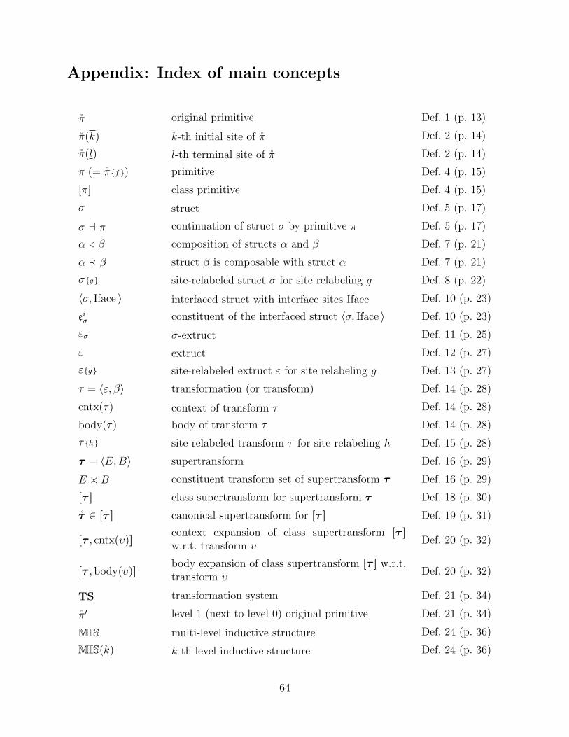
Appendix: Index of main concepts

π̊ original primitive Def. 1 (p. 13)

π̊(k) k-th initial site of π̊ Def. 2 (p. 14)

π̊(l) l-th terminal site of π̊ Def. 2 (p. 14)

π (= π̊{f }) primitive Def. 4 (p. 15)

[π] class primitive Def. 4 (p. 15)

σ struct Def. 5 (p. 17)

σ a π continuation of struct σ by primitive π Def. 5 (p. 17)

α / β composition of structs α and β Def. 7 (p. 21)

α � β struct β is composable with struct α Def. 7 (p. 21)

σ{g } site-relabeled struct σ for site relabeling g Def. 8 (p. 22)

〈σ, Iface 〉 interfaced struct with interface sites Iface Def. 10 (p. 23)

eiσ constituent of the interfaced struct 〈σ, Iface 〉 Def. 10 (p. 23)

εσ σ-extruct Def. 11 (p. 25)

ε extruct Def. 12 (p. 27)

ε{g } site-relabeled extruct ε for site relabeling g Def. 13 (p. 27)

τ = 〈ε, β〉 transformation (or transform) Def. 14 (p. 28)

cntx(τ) context of transform τ Def. 14 (p. 28)

body(τ) body of transform τ Def. 14 (p. 28)

τ {h} site-relabeled transform τ for site relabeling h Def. 15 (p. 28)

τ = 〈E, B〉 supertransform Def. 16 (p. 29)

E ×B constituent transform set of supertransform τ Def. 16 (p. 29)

[τ ] class supertransform for supertransform τ Def. 18 (p. 30)

τ̊ ∈ [τ ] canonical supertransform for [τ ] Def. 19 (p. 31)

[τ , cntx(υ)]context expansion of class supertransform [τ ]w.r.t. transform υ

Def. 20 (p. 32)

[τ , body(υ)]body expansion of class supertransform [τ ] w.r.t.transform υ

Def. 20 (p. 32)

TS transformation system Def. 21 (p. 34)

π̊′ level 1 (next to level 0) original primitive Def. 21 (p. 34)

MIS multi-level inductive structure Def. 24 (p. 36)

MIS(k) k-th level inductive structure Def. 24 (p. 36)

64

ε l σ extruct ε has just appeared in struct σ Def. 25 (p. 39)

T appl(σ(k))

the set of all k-th level canonical supertransformsthat are currently applicable to struct σ(k) Def. 26 (p. 40)

τ l σ transform τ has just appeared in struct σ Def. 27 (p. 40)

CB τ̊

context-body association strength scheme forclass supertransform [τ ] with canonical super-transform τ̊

Def. 28 (p. 41)

CLASS [τ ] class representation for class supertransform τ̊ Def. 29 (p. 42)

LEGAL set of admissible site pairs Def. 30 (p. 42)

AS primitive association strength scheme (PASS) Def. 30 (p. 42)

AS [σ a π] continuation strength scheme for σ a π Def. 31 (p. 43)

STRN(σ a π, AS) strength of the continuation of struct σ by π Def. 31 (p. 43)

qA

y mapping obtained by normalizing mapping A de-fined on set LEGAL Notation (p. 42)

c1 L1

�+ c2 L2

weighted sum of normalized mappings L1, L2 Def. 32 (p. 44)

I cntx(τ) indicator mapping for the context of τ Def. 33 (p. 45)

I body(τ) indicator mapping for the body of τ Def. 33 (p. 45)

state P(k) k-th level state of intelligent process P Def. 34 (p. 47)

WMPstate (k) k-th level working memory of process P Def. 34 (p. 47)

σ(k)state working struct (in WMP

state (k)) Def. 34 (p. 47)

AMPstate (k) k-th level association memory of process P Def. 34 (p. 47)

state P state of process P Def. 35 (p. 48)

STATE P observable state of process P Def. 35 (p. 48)

Fitcntx(τ) fitness of the context of transform τ Def. 36 (p. 49)

Fitbody(τ) fitness of the body of transform τ Def. 36 (p. 49)

T(k)avail

(stateP(k)

) the set of all transforms that have just becomeavailable in stateP(k)

Def. 37 (p. 49)

65