What have we learned from the Case Histories · slide 1 What have we learned from the Case Histories Earth materials have a range of physical properties. Application of geophysics

slide 1

What have we learned from the Case Histories

Earth materials have a range of physical properties.

Application of geophysics is carried out in a 7 Step process. Physical property of the target must be different from host material

Knowledge of a single physical property does not uniquely identify a material. Interpretation was aided by using multiple surveys.

Examples:

Gravel quaries: conductivity, elastic parameters

Karst investigations: density, conductivity

Mining: conductivity, chargeability

slide 2

MAGNETIC SURVEYING

slide 3

Geoscientific /

Engineering

Question

What is the

problem to be

solved?

Geophysics:

•Survey

•Data

•Processing

•Inversion

Formulate problem in terms

of physical properties

Interpret geophysical results

Physical

Properties

Principles for using Geophysics

slide 4

Magnetic Survey

slide 5

Some motivating examples for the use of

magnetic susceptibility

Geologic mapping

Ore deposits

Geotechnical problems

Unexploded ordnance

Buried foundations

Archeology

slide 6

Need for Magnetics: Geologic mapping

Geology contacts can be inferred from mag

maps.

Geology map Magnetic map

30 km

N N

-168.4

-133.9

-117.9

-106.3

-97.3

-90.0

-83.2

-77.2

-71.9

-66.7

-62.2

-57.5

-53.2

-48.7

-44.5

-40.5

-36.7

-32.8

-29.1

-25.1

-20.6

-15.9

-11.1

-6.0

-0.4

6.2

13.3

21.0

29.8

40.3

52.2

65.3

81.1

99.7

123.3

154.7

211.3

329.5

nT

slide 7

Need for magnetics: Mineral exploration

slide 8

Need for Magnetics: UXO

nT

-200

-100

0

100

200

Easting (m)

Nort

hin

g (

m)

0 10 20 30 40 500

10

20

30

40

50

slide 9

Magnetic materials and Magnetization

Earth materials are built up of minerals that

behave as small magnets

slide 10

Bar Magnet

North pole and South pole (dipole)

Dipole moment m is related to the strength of

the magnet

Field lines extend from the north pole to the

south polesSlide 10

slide 11

Magnetic materials and Magnetization

Earth materials are built up of minerals that

behave as small magnets

Strength of each magnet is given by the magnetic moment

Magnetization

Units: A/m dipole moment per unit volume

When the particles are randomly distributed M can be zero

slide 12

Small magnets in presence of large ones

Opposite poles attract

Like poles repel

Small magnets align

with fields of a larger

magnet

slide 13

Magnetic Susceptibility:

Ability for a rock to become “magnetized” when an

external magnetic field is applied.

Units: dimensionless

Magnetization:

Units: Dipole moment per unit volume

slide 14

Magnetic Susceptibility of Rocks

http://gpg.geosci.xyz/en/latest/content/magnetics/magnetics_susceptibility.html

slide 15

Magnetic Survey

slide 16

Geomagnetic

dynamo.

Complicated inside

the earth near the

core.

Outside the earth it

looks like a magnetic

field due to a dipole.

Earth’s Magnetic field

slide 17

Magnetics – Earth’s field

slide 18

Magnetic fields and definitions

slide 19


Link to GPG

How is the field described anywhere?

X, Y, Z

Inclination, Declination, Magnitude

Compass? Inclination?

Declination?

Earth’s field strength vs. anomalies.

http://gpg.geosci.xyz/en/latest/content/magnetics/magnetics_earths_field.html

slide 20

Earth’s Magnetic Field

slide 21

Bmax = 70,000 nT Hmax = 55.7A/m

Bmin = 20,000 nT Hmin = 15.9A/m

Total Field Strength (nT)

http://www.ngdc.noaa.gov/cgi-bin/seg/gmag/igrfpg.pl

Earth’s magnetic field: Strength |B| Inclination I Declination D

Inclination (degrees)

Declination (degrees)

slide 22

Magnetic Survey

slide 23

Basics of Magnetics Surveying

Earth’s magnetic field is the source:

Materials in the earth become magnetized

(dipole moment per unit volume)

Magnetized rocks create anomalous

(compact object looks like a magnetic dipole)

The anomalous field is a vector. To view we

project it onto specific directions (x, y, z)

slide 24

Magnetic Applet

slide 25

Simulating the field due to prisms

Interactive and live …

click here

http://mybinder.org/repo/ubcgif/gpgLabs/notebooks/Mag/InducedMag2D.ipynb

slide 26

Learning from the applet

Locating the prism at the pole and equator

Plotting Bx,By,Bz fields (sign convention: positive

when pointing in direction of axis)

Map data

Profile

Profile over a magnetic dipole.

Effects of depth of burial (half width)

Data sampling

slide 27

Survey Acquisition (with applet)

Must sample data sufficiently often to capture

the anomaly.

Want 3-5 points in a halfwidth

Width of the signal increases with depth of

burial.

Ground surveys generally choose line spacing

and station spacing to be equal.

slide 28

Magnetic Survey

slide 29

Magnetic Sensors to acquire data

slide 30

In-class magnetic surveying: Detection

Magnetic material underneath the table tops.

NO PEEKING!!!!

Use magnetic compass on smartphones (download apps if not already done)

Carry out a survey to detect the magnetic bodies.

Flag them with tape.

slide 31

If the magnet was a UXO

Magnet:

diameter: 6mm;

UXO

20cm in diameter…

If our table: ~ 1m X 3m

how large would a survey area equivalent to the table be?

Length scale ratio ~1:33

Survey area ~ 10m x 30m

slide 32


20cm in diameter…

how large would a survey area equivalent to the table be?

slide 33


20cm in diameter

slide 34

Team Exercise: Searching for $1B Cu deposit

Magnet: diameter: 6mm; height=2mm vol 5.65e-8 m^3

For table size: ~ 1m X 3m

Price: $310 USD/lb; $684 /kg

$1 billion. I need: ??? Kg

Density of copper 8960 kg/m^3

Need ??? m^3 of copper

Assume 0.3% Cu by volume: ??? m^3

Scale length of deposit: 1 ~ ????

Survey area: ?? km x ?? km

slide 35

Student exercise

Magnet: diameter: 6mm; height=2mm vol 5.65e-8 m^3

Table: 1m x 3m

Find a copper resource worth $1B

Price: $3.10 USD/lb; $6.84 /kg (Note decimal)

$1 billion 1,461,305 kg

Density of copper 8960 kg/m^3

Need 163 m^3 of copper

Assume 0.3% Cu by volume: 54,330 m^3 (cube: 38 m on side)

Scale length:

Survey area: 10 km x 30 km

slide 36

If the magnet was a billion dollar copper deposit

slide 37

Readings

GPG Magnetics

Lab #2 (see course website)

../../EOSC350_FJ/homepage/content/index.htm

slide 38

The composite field

Composite field:

B = B0 + BA

B0

BAB is a vector:

B = {Bx, By, Bz}

Total field:

|B| = |B0 + BA|

slide 39

The Anomalous field

The total field anomaly: B = |B| - |B0|

If |BA| << |B0| then

That is, total field anomaly B is the projection of the anomalous

field onto the direction of the inducing field.

B0

BAMeasured field B = B0 + BA

Link to GPG

http://gpg.geosci.xyz/en/latest/content/magnetics/magnetics_earths_field.html

slide 40

Vector Diagram

Why is the total field anomaly:

BA

B0

B

|B|-|BA|

|BA|cos

slide 41

Learning from the applet:

Locating the prism at the pole and equator

Plotting total field anomaly (sign convention:

positive in direction of Earths’ field)

Map data

Profile

Profile over a magnetic dipole.

Effects of depth of burial (half width)

Data sampling

slide 42

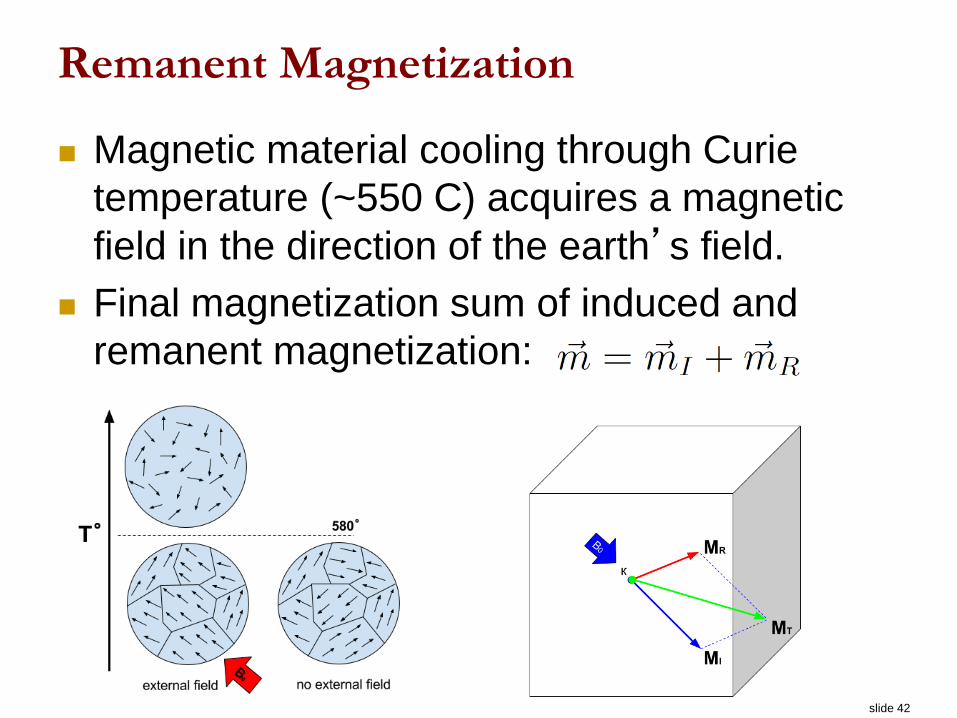
Remanent Magnetization

Magnetic material cooling through Curie

temperature (~550 C) acquires a magnetic

field in the direction of the earth’s field.

Final magnetization sum of induced and

remanent magnetization:

slide 43

Remanent Magnetism at different scales

Small scale: UXO, rebar,

drums

Large scale: geologic

units.

Sea floor spreading

slide 44

Magnetic map of North America http://pubs.usgs.gov/sm/mag_map/mag_s.pdf

http://pubs.usgs.gov/sm/mag_map/mag_s.pdf

slide 45

Notebook App:

A single prism with uniform magnetization

Arbitrary dimensions

Arbitrary orientation of the body

Arbitrary strength and orientation of remanent

magnetization.

Can model cubes, rods, sheets, dykes …

slide 46

Find by digging

slide 47

Work as a team

slide 48

But geophysics may be more efficient

and easier!

slide 49

But geophysics may be more efficient

and easier!

slide 50

Data Processing

Removing time variations of the Earth’s field

(necessity for a base station)

Removing a regional trend

Slide 50

slide 51

Slide 51


slide 52

Time Variations of the Earth’s Field

External sources

Solar wind (micro-seconds, minutes, hours)

Solar storms (hours, days, months)

Man made sources

Power lines (50/60 Hz plus harmonics) DC

Motors, generators

All electronic equipment

Internal sources

Fluctuations in core (days – millions of years)

slide 53

Time variations due to a magnetic storm

Adapted from NRC http://www.spaceweather.gc.ca/tech/se-pip-en.php

slide 54

Field procedures

Earth’s magnetic field varies as a function of

time

Necessary to record the magnetic field at a

fixed location to determine the Earth’s field

slide 55

Base station correction

Set out another magnetometer (base station)

Assume time variations at the base stations

are the same as at the observation location

Synchronize the times

Perform a correction by subtraction

slide 56

Anomalous field

We measure the field at the Earth’s surface

but we are interested in the “anomalous”

features

Estimate a region and subtract

Regional removal (along a line)

Regional removal (for a plane of data)

slide 57

Removing a background field

Background field is generally anything that is smoothly

varying over your region of interest and is much larger

than the footprint of the body you are interested in.

Deciding what is background is a subjective decision.

slide 58

Regional field removal for map data

Airborne magnetic data gathered over a 25 square km area around a mineral

deposit in central British Columbia. Some geological structural information is

shown as black lines. The monzonite stock in the centre of the boxed region

is a magnetic body, but this is not very clear in the data before removing the

regional trend.

slide 59

These are the data that we want to use to

extract information about our problem.

Examples of magnetic anomaly data

slide 60

Status Slide

Now have all of the material needed for the

lab

slide 61

Possible routes to extracting information

Inference from data images.

Interpret with a simple body of uniform

magnetization (monopole, dipole, dyke)

Interpret as complex body (inversion)

slide 62

Inferences from data images

Magnetic signatures are complicated because the same

object provides different data depending where it on the

earth (ie depends upon strength and direction of the

inducing field.

Applet example

This ambiguity can be reduced by processing the data

by “Reducing to the Pole”

slide 63

Reduction to Pole

Same object buried at different locations on the earth yields different total field anomalies.

Inclination=0 Inclination=45 Inclination=90

slide 64

Reduction to Pole

Filter the data to emulate the response as if the survey was taken at the pole. (Earth’s field is vertical; measure vertical component of the anomalous field)

2D Fourier Filter

→

This simplifies interpretation. Causative body lies beneath the peak.

slide 65




magnetization (dipole, dyke, monopole)


slide 66

Remanent Magnetization:

A complicating factor…..

These look like dipoles

but directions are not

in consistent direction.

nT

-200

-100

0

100

200

Easting (m)

Nort

hin

g (

m)

0 10 20 30 40 500

10

20

30

40

50

slide 67

Parameter Estimation: UXO as a Dipole

We model the response as a dipole (equivalent

to a bar-magnet):

Position

Depth

Orientation

Size

6 parameters

slide 68

Parameter extraction

Six parameters ( [x,y,z, strength and orientation of dipole])

Inversion or “parameter extraction” is used to estimate the

parameters of an underlying model

Sensor data: d

Model Parameters: md =g [m]

m=g-1 [d ]

Forward Operator

Inverse Operator

slide 69

Easting = -0.13 m

Northing = 0.16 m

Depth = 0.26 m

Moment = 0.0226 Am2

Azimuth = 37o

Dip = 28.8o

Fit quality = 0.95

Parameter extractionDATA PREDICTED DATA

Residuals

Parameters

of interest

slide 70






slide 71

Modelling objects with uniform

magnetization.

Simplification by working with charges.

slide 72

Magnetic Monopole (GPG-Basic Principles)

Charges generate a magnetic field B

Q

-Q

slide 73

Magnetic Dipole

In nature: magnetic poles always appear in pairs with a positive and negative

pole yielding a dipole.

Magnetic moment

Magnetic field of dipole

Q

-Q

L

m

slide 74

Slide 74

Beyond dipoles – real targets

When is a buried feature like a simple dipole?

When it’s diameter is much less than depth to it’s centre.

GPG Magnetics: Basic Principles

Fields from some buried bodies, (cylinders, dykes) can be

estimated by using charge concepts.

Charge strength, τ = n̂ M

slide 75

A simple model for a vertical pipe



(Magnetization)

Q -

slide 76

A simple model for a vertical pipe



A vertical pipe has anomaly like a single pole.(TBL 2)

Q -

slide 77

Magnetic fields from an extended pipe

For the lab

For the TBL

Connect with GPG

Connection with amplitude of anomaly

Width of anomaly and depth of burial

slide 78






slide 79

Superposition for Magnetics Data (GPG d5)

Magnetic field for one prism

Prism own dipole fieldMagnetic field for 5 prisms

Superposition

slide 80

Earth can be complicated

A complicated earth model Magnetic data for a complicated

earth model.

To interpret field data from a complicated earth we need to have

formal inversion procedures that recognize non-uniqueness.

Think about finding the causative magnetization of each prism.

slide 81

Slide 81

Example: Raglan aeromagnetic data

Select a region of interest.

Keep data set size within reason.

Digitized the Earth – up to 106 cells.

slide 82

Slide 82

Inversion:

Finding an earth model that generated the data

Inversion

?

Divide the earth into many cells of constant but unknown susceptibility

Solve the large inverse problem to estimate the value of each cell

slide 83

Slide 83

Misfit: comparing predictions to measurements

Once a model is estimated …

Compare

Compare predictions to

these measurements.

Calculate data caused by that model.

Proceed to check for acceptibility

Modify model and try again

Is comparison within errors?

YES NO

slide 84

Slide 84

? ?

• Are “sills” connected at depth? Inversion result supports this idea.

• It helped justify a 1050m drill hole.

• 330m of peridotite intersected at 650m 10m were ore grade.

• Image shows all material which has k > 0.04 SI.

Estimate a model for the distribution of subsurface magnetic material.

Model will be “smooth”, and close to pre-defined reference.

Display result as cross sections and as isosurfaces.

Raglan aeromagnetic data

slide 85

APPLICATIONS

slide 86

Geoscientific /

Engineering

Question

What is the

problem to be

solved?

Geophysics:

•Survey

•Data

•Processing

•Inversion

Formulate problem in terms

of physical properties

Interpret geophysical results

Physical

Properties

Principles for using Geophysics

slide 87

Framework for Applied Geophysics:

7 Steps

slide 88

Some motivating examples for the use of

magnetic susceptibility

Geologic mapping

Ore deposits

Geotechnical problems

Unexploded ordnance

Buried foundations

Archeology

Slide 88

slide 89




magnetization (monopole, dipole, dyke)


slide 90

Magnetics for Geologic Mapping

When rock outcrops are sparse we must rely on other available

techniques to denote changes in geologic units and/or structures.

Geology unit A ? Geology unit B ?

slide 91

Magnetic surveys

Very common mineral exploration tool to aid with geologic mapping.

One of the cheapest geophysical surveys to execute on land or with an aircraft.

Used on regional and deposit scale to identify geologic boundaries and structures (such as faults or folds).

Many mineral deposits are found on geology boundaries or faults so magnetic maps are useful for target prospective areas.

slide 92

Geologic boundaries

Geology contacts can be inferred from mag

maps.


30 km

N N

-168.4

-133.9

-117.9

-106.3

-97.3

-90.0

-83.2

-77.2

-71.9

-66.7

-62.2

-57.5

-53.2

-48.7

-44.5

-40.5

-36.7

-32.8

-29.1

-25.1

-20.6

-15.9

-11.1

-6.0

-0.4

6.2

13.3

21.0

29.8

40.3

52.2

65.3

81.1

99.7

123.3

154.7

211.3

329.5

nT

slide 93

Identifying regional scale faults

Mag map highlights faults within known gold

bearing plutonic body (red) in west-central Yukon.

55 km


N N

slide 94

Example - Iron ore deposit

Magnetite rich rock shows as mag high anomaly

slide 95

Other processing

Vertical/horizontal derivative maps

Mount Dore, Australia

Slide 95

slide 96410,000 440,000 470,000

Easting (m)

7,5

80,0

00

7,6

20,0

00

7,6

60,0

00

No

rth

ing

( m

)

Landsat

Image

Topography

Mount Dore, Queensland, Australia

Surface Geology

410,000 440,000 470,000

Easting (m)410,000 440,000

Easting (m)

Source: Queensland Government, Australia

slide 97410,000 440,000 470,000

Easting (m)

7,5

80,0

00

7,6

20,0

00

7,6

60,0

00

No

rth

ing

( m

)

410,000 440,000 470,000

Easting (m)410,000 440,000

Easting (m)

Magnetic data

Total Magnetic Anomaly

(nT)

1th Vertical Derivative

Source: Queensland Government, Australia

slide 98






slide 99

The Munitions Problem

There are over 3,000 sites suspected of

contamination with military munitions

They comprise 10s of millions of acres

The current annual cleanup effort is on the

order of 1% of the projected total cost

To make real progress on this problem, we

need a better approach

slide 100


slide 101


slide 102


slide 103


slide 104


slide 105

Environmental: How do we find UXO?

?

slide 106

Environmental : Magnetic Survey

TM4

Ferrex

nT

-200

-100

0

100

200

Easting (m)

Nort

hin

g (

m)

0 10 20 30 40 500

10

20

30

40

50

slide 107

Examples of “good” data

High SNRMedium SNR

Medium SNR Low SNR

Easting (m)

Easting (m)Easting (m)

Easting (m)

No

rth

ing

(m

)N

ort

hin

g (

m)

No

rth

ing

(m

)N

ort

hin

g (

m)

210 nT

-140 nT

22 nT

-21 nT

4.3 nT

-2.7 nT

8.5 nT

-7.5 nT

slide 108

What is the formula for a magnetic dipole

These look like dipoles but how do we

analyze the signal?

EOSC 350 ‘06

Slide 108

nT

-200

-100

0

100

200

Easting (m)

Nort

hin

g (

m)

0 10 20 30 40 500

10

20

30

40

50

slide 109

The model

We model the response of buried items by a

dipole (equivalent to a bar-magnet):

Position

Depth

Orientation

Size

6 parameters

DEPTH

Position

slide 110

Parameter extraction

Need six parameters (location, strength and orientation)

Inversion or “parameter extraction” is used to estimate

the parameters of an underlying model that encapsulates

some useful attributes of the buried object

Sensor data: d

Model Parameters: md =g [m]

m=g-1 [d ]

Forward Operator

Inverse Operator

slide 111

Easting = -0.13 m

Northing = 0.16 m

Depth = 0.26 m

Moment = 0.0226 Am2

Azimuth = 37o

Dip = 28.8o

Fit quality = 0.95

Parameter extractionDATA PREDICTED DATA

Residuals

Parameters

of interest

slide 112

Magnetics

Parameter extractionConcepts

Real-world examples

Magnetics fundamentalsSensor systems

Data examples and demo

ClassificationUsing the parameters to make

discrimination decisions

EM surveys

will also be

needed.

slide 113






slide 114

Ekati Property, Northwest Territories

slide 115


slide 116


slide 117


slide 118

Misery Pipe

Borrowed from Nowicki et al. (2004)

• Property owned by BHP Billiton

• Pre-stripping under way

• Production expected to start in 2016

slide 119

Misery Pipe

• Local anomaly showing reversely magnetized body

• Removal of the regional field to enhance the target

slide 121

Misery Pipe

• Magnetic Inversion

Borrowed from Nowicki et al. (2004)

Inverted modelGeology from drilling

slide 122

Slide 122

Summary: Magnetics – interpretation

1. Qualitative: Correlate magnetic patterns to geology

2. Quantitative interpretation Determine shapes, volumes, contacts, materials

3. Direct interpretation of patterns

4. Forward modelling1. “Guess” geology

2. Calculate result - Compare to data

3. Iterate.

5. Inversion: Given data, estimate possible configurations of susceptible material that could cause those data.

slide 123

The End of Magnetics

Slide 123

Documents

What have we learned from the Case Histories · slide 1 What have we learned from the Case Histories Earth materials have a range of physical properties. Application of geophysics