Policy Research Working Paper 8303

What Explains the Gender Gap Reversal in Educational Attainment?

Laurent BossavieOhto Kanninen

Social Protection and Labor Global Practice GroupJanuary 2018

Pub

lic D

iscl

osur

e A

utho

rized

Pub

lic D

iscl

osur

e A

utho

rized

Pub

lic D

iscl

osur

e A

utho

rized

Pub

lic D

iscl

osur

e A

utho

rized

Produced by the Research Support Team

Abstract

The Policy Research Working Paper Series disseminates the findings of work in progress to encourage the exchange of ideas about development issues. An objective of the series is to get the findings out quickly, even if the presentations are less than fully polished. The papers carry the names of the authors and should be cited accordingly. The findings, interpretations, and conclusions expressed in this paper are entirely those of the authors. They do not necessarily represent the views of the International Bank for Reconstruction and Development/World Bank and its affiliated organizations, or those of the Executive Directors of the World Bank or the governments they represent.

Policy Research Working Paper 8303

This paper is a product of the Social Protection and Labor Global Practice Group. It is part of a larger effort by the World Bank to provide open access to its research and make a contribution to development policy discussions around the world. Policy Research Working Papers are also posted on the Web at http://econ.worldbank.org. The authors may be contacted at lbossavie@worldbank.org.

The reversal of the gender gap in educational attainment is becoming a global phenomenon. Its drivers, however, are not well understood and remain largely untested empiri-cally. This paper develops a unified conceptual framework that allows to formulate and test two main hypotheses for the reversal. It introduces the tail hypothesis, which builds on the lower dispersion of scholastic performance among females observed globally. It also formalizes the mean hypothesis, which states that females’ average scho-lastic performance and returns to education have increased over time relative to males’. The paper theoretically shows

that both hypotheses can explain the reversal in our framework. The parameters of the two hypotheses derived from the model are then estimated using educational attainment data from 1950 to 2010 in more than 100 countries. The authors find that both hypotheses strongly predict the gender gap dynamics in educational attain-ment when estimated separately. When jointly estimated, accounting for the tail hypothesis significantly increases the model’s predictive power. The contribution of the tail hypothesis to the gender gap reversal, while the mean hypothesis appears to prevail in high-income countries.

What Explains the Gender Gap Reversal in Educational Attainment?∗

Laurent Bossavie†and Ohto Kanninen‡

Keywords: Educational attainment, gender gap, gender differences in scholastic performance.

JEL-Codes: I20, J16

∗We would like to thank Jerôme Adda, Christian Dustmann, Nicole Fortin, Paola Giuliano, Luigi Guiso, PeterHansen, Andrea Ichino, Steve Machin, Tommaso Naniccini, Tuomas Pekkarinen, Kjell Salvanes, Uta Shoenberg andOlmo Silva as well as participants to various conferences and workshops for helpful comments and suggestions. Theviews expressed in the paper are enitrely those of the authors, they do not necessarily represent the views of theInternational Bank for Reconstruction and Development /World Bank and its affiliated institutions or those of theexecutive directors of the World Bank of the governments they represent.

†The World Bank. Corresponding author. E-mail: lbossavie@worldbank.org. Address: The Word Bank, 1818 HStreet NW, 20433 Washington DC, USA. Phone: +1 202-751-6478.

‡Labour Institute for Economic Research (LIER), Helsinki.

1 Introduction

The dramatic increase in educational attainment over the past decades was accompanied by a

striking and puzzling phenomenon. As individuals stayed longer in school over time, females not

only caught up with males’ education levels, but progressively attained higher levels of schooling.

This phenomenon, sometimes referred to as the gender gap reversal in education, already took

place in virtually all high-income countries. It is also observed in a growing majority of low and

middle-income countries. Although the reversal is becoming close to universal, its origins are not

well understood.

A lot of attention in the literature has been devoted to explaining the gender gap in labor market

market outcomes. In contrast, the gender gap reversal in educational attainment has been under-

studied. A few contributions, confined to the US context, have proposed possible explanations for

this phenomenon (Goldin, Katz and Kuziemko 2006; Cho 2007; Chiappori, Iyigun and Weiss 2009

and Fortin, Oreopoulos and Phipps 2015). However, to the best of our knowledge, there has been

no attempt to model and test alternative hypotheses for this reversal using a unified conceptual

framework. This paper aims at filling this gap.

Understanding the origins of the educational gender gap reversal is important in itself, but also to

explain gender dynamics in other areas, particularly in the labor market. For policy purposes, it is

also important to identify whether differences in educational outcomes between genders originate

from distortions such as social barriers and discrimination or, instead, from optimizing behaviors

based on potential gender differences in preferences or traits.1 Learning about the origins of the

gender gap reversal can help determine whether policy interventions could help addressing the

growing disadvantage of boys in school, and identify potential areas of interventions.

The paper starts by establishing that the gender gap reversal in education is becoming a global phe-

nomenon. Using time-series on enrollment and completion rates in education by gender in more

than 100 countries, we show that the reversal occurred in virtually all high-income countries, but

also in a rapidly growing proportion of lower-income countries. We also evidence that the reversal1For a summary of evidence on gender differences in preferences, see Croson and Gneezy (2009).

2

is not confined to tertiary enrollment as evidenced by previous literature, but also took place at the

primary and secondary level.2 While females have historically represented the minority of tertiary,

secondary and primary education completers, they have become the majority over time.

The second contribution of the paper is to develop a simple conceptual framework to account

for the gender gap reversal in educational attainment. In our framework, differences in the dis-

tributions of scholastic performance between genders play a central role.3 The model builds on

the micro foundations of investment in schooling of Card (1994), before aggregating individual

schooling decisions to the macro level. It has three building blocks. First, at the micro level,

the optimal number of years of schooling attained by individuals increases with their scholastic

performance. Second, the benefits of investing in schooling are allowed to vary over time and

between genders. Third, we introduce two alternative assumptions regarding the distribution of

scholastic performance by gender. These distributional assumptions, together with an increase in

the economy-wide benefits of investing in schooling, generate either a tail dynamics or a mean

dynamics, depending on the assumption made. Our model allows to combine these two dynamics

within a unified conceptual framework.

A central contribution of the paper is to propose and model the tail dynamics hypothesis within our

conceptual framework, and to show that it can generate the gender gap reversal in education. A

key result of our model under the tail hypothesis is that a higher variance in scholastic performance

among males is sufficient to produce the gender gap reversal, independently of the relative mean

scholastic performance of males and females. We show that the tail hypothesis implies first a

gender gap reversal in favor of females, but ultimately gender equality in educational attainment as

the net benefits of education increase over time and enrollment becomes universal. The hypothesis

is novel in the literature and builds on the findings of Machin and Pekkarinen (2008) who find that

girls exhibit a lower variance in mathematics and reading test scores relative to boys in virtually

all OECD countries.4 It also formalizes the intuition of Becker, Hubbard and Murphy (2010a) and2The latter applies mostly to low-income countries.3In the remainder of the paper, scholastic performance refers to students’ performance in achievement tests as

measured by standardized test scores, while educational attainment refers to the highest level of schooling attained byan individual, e.g secondary school completion.

4There also exists an abundant literature in psychology reporting similar findings for different dimensions of abili-ties or traits, such as Frasier (1919), Hedges and Nowell (1995), or Jacob (2002), among many others.

3

Becker, Hubbard and Murphy (2010b), who suggest that the lower variance of non-cognitive skills

among females can generate a higher elasticity of enrollment to returns to schooling.

We also model the mean dynamics hypothesis within our framework. Contrary to the tail hypoth-

esis, the predictions of the mean hypothesis depend directly on the dynamics of gender-specific

means, and gender equality in educational attainment is only achieved if gender-specific means

are the same. The mean dynamics hypothesis can be modeled in two alternative ways within our

framework. It first can be formalized through the mean benefit hypothesis (MBH), which posits

that the net benefits of schooling for females have increased more rapidly over time than for males

(Goldin, Katz and Kuziemko 2006 and Chiappori, Iyigun and Weiss 2009). Second, it can be mod-

eled through the mean performance hypothesis (MPH), which claims that the mean performance

of females in achievement tests has increased over time relative to males’ (Cho 2007). We show

that both hypotheses are algebraically similar in our framework, and can produce a reversal of the

gender gap in educational attainment.

A final contribution of the paper is empirical. Building on our conceptual framework, we are able

to estimate the respective contributions of the two hypotheses to the gender gap reversal. This is,

to the best of our knowledge, the first paper that formally quantifies the contributions of alternative

hypotheses within a unified framework. Using our model, we show that each of the mean and tail

dynamics hypothesis can be expressed by a reduced-form equation and summarized by two key

parameters. We then fit each hypothesis using harmonized time-series data on educational attain-

ment by gender from 1950 to 2010 in a large sample of countries. We estimate each hypothesis’

parameters derived from our theoretical framework first separately, and then jointly.

We find that the model under either parameter strongly predicts the dynamics of the gender gap in

tertiary enrollment in the full sample. Accounting for both parameters in the estimation strongly

increases predictive power, as opposed to specifications with only one of the two hypotheses pa-

rameters. For secondary school completion, however, the predictive power of the mean hypothesis

is lower than that of the tail hypothesis in the full sample. Once we split our sample between

developing and high-income countries, we find that the respective explanatory power of the two

hypotheses varies in the two groups. While the tail hypothesis predominates in the developing

4

country sample, the mean hypothesis has stronger explanatory power in the high-income country

sample.

Our findings indicate that while the tail and mean dynamics have both been at play, the former has

a strong and independent explanatory power that has not been uncovered by previous literature,

especially in the context of developing economies. Our model estimates for the tail hypothesis

parameter are also close to the male-to-female variance ratio in test scores estimated from inter-

national student assessments. In addition, our model parameter estimates are fairly robust across

specifications. This provides further comfort on the validity of the tail hypothesis in accounting

for the gender gap reversal in educational attainment.

The paper is organized as follows. Section 2 presents empirical facts on the gender gap reversal

in educational attainment that motivate the paper. Section 3 lays out our conceptual framework.

Section 4 formulates two main hypotheses for the gender gap reversal within this framework.

Section 5 describes our empirical methodology to estimate the contribution of the two hypotheses

to the gender gap reversal. Section 6 presents our empirical results and discusses their implications.

Section 7 concludes.

2 Empirical Motivation

2.1 Data

The data used throughout the paper is from the Barro-Lee educational attainment database. The

dataset consists of harmonized country-level data on educational attainment constructed from na-

tionally representative surveys and census data. The data is reported at five-year intervals from

1950 and 2010. It is also disaggregated into five-year age groups. The availability of age-specific

data is valuable in our context, as it allows to construct the dynamics of educational attainment of

specific age cohorts over time. Educational attainment is also reported separately for males and

females, which allows to follow the evolution of educational attainment across cohorts by gender.

Time-series of educational attainment are available for a total of 146 countries in the database,

5

which include 36 OECD economies and 110 non-OECD countries.5 Educational attainment of

the adult population in the database is broken down into seven levels of schooling: no formal

education, incomplete primary, complete primary, lower secondary, upper secondary, incomplete

tertiary, and complete tertiary.

To describe time trends in educational attainment by gender, we focus on three main levels of

educational attainment: primary school completion, secondary school completion, and enrollment

in tertiary education. As the data is reported every five years from 1950 to 2010, we have a

maximum of 13 data points per country, for a given level of educational attainment. We exclude

eight countries from the original Barro-Lee dataset, due to highly inconsistent data and missing

values on educational attainment.6

We compute completion and enrollment rates for 5-year-band birth cohorts born from 1921 to

1990, by gender.7 We measure the enrollment rate in tertiary education at time t as the share of

the population age 25-29 that has ever enrolled in tertiary education. The secondary education

completion rate is measured as the share of the population age 20-24 at time t that has completed

secondary education and above. Finally, primary education completion rates are measured as the

share of the population age 15-19 at time t that has completed primary education and above.8 The

female-to-male ratio is measured as the enrollment or completion rate of females over that of males

for a given level of educational attainment.

Table I displays the summary statistics of enrollment and completion rates for primary, secondary

and tertiary education in OECD and non-OECD countries from the Barro-Lee database in 1950

and 2010. As documented in Barro and Lee (2013) and Lee and Lee (2016), the data shows a large

increase in educational attainment over the period covered. In addition, and more importantly in

the context of the paper, enrollment and completion rates have increased more rapidly for females5In case of missing observations over time, data points were obtained by forward and backward extrapolation of

the census/survey observations on attainment. See Barro and Lee (2013) and Lee and Lee (2016) for a completedescription of the dataset construction and methodology.

6Excluded countries are Bostwana, Burundi, Cameroon, Gabon, Guyana, Mozambique, Libya and Yemen.7For primary education, we compute completion rates for individuals born between 1936 to 1995, from 1931 to

1990 for secondary school completion and from 1921 to 1980 for tertiary education.8The choice of these age brackets was motived by the fact that individuals would be expected to have enrolled in

or completed the corresponding level of education by these ages, if they ever did.

6

than for males for all three levels of educational attainment. This pattern is observed in both OECD

and non-OECD countries.

2.2 The Gender Gap Reversal in Educational Attainment

Several papers have reported a convergence followed by a reversal in the relative number of fe-

males attending tertiary education in the US (Charles and Luoh 2003; Goldin, Katz and Kuziemko

2006, Chiappori, Iyigun and Weiss 2009; Becker, Hubbard and Murphy 2010a; Becker, Hub-

bard and Murphy 2010b; Autor and Wasserman 2013).9 In table II and Figure I, we look at the

evolution of the female-to-male ratio in tertiary enrollment worldwide, by grouping country-level

data into seven world regions.10 As shown in Column 5 and 6 of Table II, young males in 1950

used to outnumber females among participants to tertiary education in virtually all countries in

the sample (92%). In contrast, by 2010, 73% of countries in the sample had seen their gender

imbalances in tertiary enrollment revert from a male majority to a female majority. Even among

non-OECD countries, 66% had experienced the gender gap reversal in tertiary enrollment by 2010.

In advanced economies, Europe and Central Asia and Latin America, the share of countries where

females outnumber males among tertiary education students is over 90%. In contrast, most coun-

tries in South Asia and Sub-saharan Africa have yet to experience the gender gap reversal in tertiary

enrollment.

When averaged over all countries in the sample, the Barro-Lee data show a reversal in the gender

gap in tertiary enrollment, as reported in Panel A of Figure I. For the oldest cohorts born in the

1920s, the average female-to-male ratio in tertiary enrollment for all countries in the sample was

around 0.40, meaning that for ten females enrolled in tertiary education, only four females were

enrolled. This ratio was fairly similar across all regions of the world. In contrast, among the most

recent cohorts, the average female-to-male ratio had reached 1.22 globally, meaning that there were

22% more females enrolled in tertiary education than males worldwide.9Pekkarinen (2012) has also reported this phenomenon for Scandinavian countries.

10This regional grouping follows the World Bank classification of world regions and includes: advanced economies,Latin American and the Caribean, Europe and Central Asia, East-Asia an Pacific, the Middle-East and North Africa,South Asia and Sub-saharan Africa

7

Out of the seven world regions, five have already crossed the horizontal line of a female-to-male ra-

tio of 1, meaning that they experienced the gender gap reversal in tertiary enrollment. Sub-saharan

African and South Asia are the only two regions that have yet to experience the reversal, with

a female-to-male ratio in tertiary enrollment remaining below one despite a noticeable increase

across cohorts.

Panel A of Figure I also shows that the timing of the reversal varies across regions. The gender

gap reversal in tertiary enrollment occurred first in Europe and Central Asia for cohorts born at

the beginning of the 1950s. In advanced economies and Latin America American countries, this

reversal occurred first for cohorts born around 1960. Among countries in East Asia and the Middle-

East and Northern Africa, the reversal only took place among cohorts born in the late 1970s.

Table II and Figure I show that the global gender gap reversal in educational attainment is not

limited to tertiary education enrollment. The gender composition of secondary school completers

has also reversed from a male majority to a female majority over time. While young females used

to outnumber males among secondary school non-completers in only 6% of the countries in the

sample in 1950, females now represent the majority of secondary school completers in 71% of

countries in the sample. As for tertiary enrollment, the gender gap reversal in secondary school

completion already occurred in five out of the seven world regions. The share of countries that have

experienced the reversal is highest in advanced economies (92%) and lowest in Subsaharan Africa

(38%). As for tertiary enrollment, Europe and Central Asia is the first region to have experienced

the gender gap reversal in secondary school completion.

Finally, we also observe a closure and reversal of the gender gap in primary school completion,

although patterns are less clear cut than for secondary and tertiary education. As shown in Panel

C of Figure I, the female-to-male ratio in primary completion averaged over all countries in the

sample was 0.82 for the oldest cohorts born at the beginning of the 1930s, but had reached a mean

of 1.03 among cohorts born at the beginning of the 1990s. When disaggregated by regions, all

regions have reached female-to-male ratios in primary school completion around or slightly above

one for the latest cohorts, with the exception of South Asia. Similarly, a majority of countries

have experienced the gender gap reversal in primary school completion in most regions (Table II).

8

The extent of the reversal is however smaller than for secondary school completion and tertiary

enrollment. Among advanced economies in particular, the share of countries that experienced the

gender gap reversal in primary school completion has hardly changed from 1950 to 2010.

The fact that the gender gap reversal is not as clear cut at the primary level could be explained by

several factors. First, in many countries in our sample, primary school completion has been close to

universal already for some time. As a result, there has been little variation in the gender ratio which

remained around one over our period of study. This is the case for advanced economies, Europe

and Central Asia and Latin America (Figure I). A related explanation is that primary schooling

has been mandatory for some time for many countries in the sample, which leaves little room for

variation in the gender ratio in primary school completion over time. As result, primary school

completion is mainly driven by institutional features rather than optimal decisions of investment in

schooling by gender.

3 Theoretical Framework

3.1 Micro Foundations

We now develop a conceptual framework that allows to formulate alternative hypotheses for the

reversal. The economy is assumed to be populated by of mass individuals that differ in their level

of scholastic performance z, which is continuous and perfectly observed by individuals.11 For the

sake of simplicity, a single-period model is assumed where individuals receive the benefits of their

investment in schooling in the same period as they invest. Individuals choose years of schooling

s to maximize their level of utility U . Building on Card (1994), we simply express the utility

function of individuals as:

U(s) = B(s)− C(s),

11Scholastic performance can be interpreted as the product of a complex combination of individual ability as wellas other inputs such as effort and motivation, which can empirically be measured by test scores (Heckman and Kautz,2012)

9

where B(s) is the benefit function of schooling, with B�(s) > 0 and B

��(s) < 0. C(s) is the

cost function of schooling, which is assumed to be increasing and convex in s. The first-order

conditions for the individual maximization problem read as:

B�(s) = C

�(s),

where B�(s) and C�(s) denote the marginal benefits and costs of schooling, respectively. Following

Card (1994), we linearize the model by assuming that B�(s) and C�(s) are linear functions of s,

with B�(s) having an individual-specific intercept:

B�(s) = zj − k1s

C�(s) = k2s,

where k1 > 0 and k2 > 0. Intuitively, individuals with higher levels of scholastic performance zj

get higher marginal benefits from schooling.12 In this framework, the optimal level of schooling s

chosen by individual j can be expressed as:

s∗j= zj · b, (1)

where b ≡ 1k1+k2

is an exogenous technology parameter, which we call net benefits of schooling

(hereafter: net benefits). It is identical for all individuals in the economy. b captures the monetary

and non-monetary benefits and costs of schooling in the economy. The optimal level of schooling

chosen by individual j is therefore strictly increasing in individual scholastic performance zj .

In this framework, the minimum level of scholastic performance z so that individuals attain a given

level of schooling s, such as tertiary education, can be expressed as:

z =s

b(2)

12In the original model of Card (1994), the expression for C’(s) also includes an individual-specific intercept, cap-turing individual-specific circumstances such as access to wealth and network or taste for education. For the sake ofsimplicity, we abstract from this distinction in our model.

10

Equation 2 states that individuals whose scholastic performance is below the threshold z attain

an optimal level of schooling below s, while individuals whose scholastic performance is equal

to or greater than z attain s and above. It also implies that the scholastic performance threshold

is determined by b, common to all individuals in a given cohort. An immediate implication of

Equation 2 is:∂z

∂b≤ 0.

In words, the minimum level of scholastic performance required to attain a given level of school-

ing s, such as tertiary education, decreases with the net benefits of investing in schooling in the

economy.

3.2 Aggregate Educational Attainment and Gender Ratio

We now assume that the economy is populated by successive cohorts. Each cohort consists of a

continuum of agents that invest in schooling and differ in their level of scholastic performance z.

Let fz(z) denote the probability density function of scholastic performance z in the population of a

given cohort. The complementary cumulative distribution function of z can be expressed as:

Gz(z) =

� +∞

z

fz(z) d(z).

All individuals belonging to the same cohort are exposed to the same value of the exogenous

parameter bt ≡ 1k1,t+k2,t

, irrespective of their scholastic performance. Given the micro properties

of the model summarized in Equation (1) and (2), the share of individuals in the cohort that attain

a level of schooling of at least s is given by:

P (z) = 1− Fz(s

b) = Gz(

s

b) = Gz(z). (3)

Equation (3) states that the mass of individuals that attain a level of schooling of at least s or

higher, for a given value of b, is made of all individuals whose scholastic performance is above the

scholastic performance threshold z. Exogenously to individual schooling decisions, b varies across

11

cohorts. Equation (3) implies:∂P (z)

∂b≥ 0.

The share of individuals that attain a level of schooling equal or higher than s therefore increases

with the net benefits of schooling b. One key implication at the aggregate level is that, as the net

benefits of schooling rise, educational attainment increases and the mean scholastic performance

of individuals that attain a given level of schooling decreases. In Appendix A1.3, we show hat this

result holds empirically, using US data.

We now introduce the possibility that Gz(.) and z differ between genders. Let zm and zf be random

variables that denote the scholastic performance of males and females, respectively. The scholastic

performance threshold z is also allowed to vary by gender and denoted zm and zf for males and

females, respectively. In our framework, the fraction of the population in the cohort that attains a

given level of schooling s, assuming the total population of males and females is the same, is given

by:

P (·) ≡Gzf

(zf ) +Gzm(zm)

2(4)

and the female-to-male ratio among individuals that choose a given level of schooling, denoted

R(z), can be expressed as:

R(·) ≡Gzf

(zf )

Gzm(zm)(5)

The implications of our model at the aggregate level are fully summarized by Equation 4 and 5.

In the remainder of the paper, Gzfand Gzm are assumed to be characterized by their first two

moments, where µ and σ2 denote the mean and variance of the distributions, respectively.

4 Two Main Hypotheses for the Gender Gap Reversal

Within this theoretical framework, we formulate two main hypotheses for the gender gap rever-

sal: the tail dynamics hypothesis (or tail hypothesis), and the mean dynamics hypothesis (or mean

hypothesis). The mean dynamics hypothesis itself can be formalized in two alternative ways:

12

through the mean performance hypothesis (MPH), or through the mean benefit hypothesis (MBH).

As shown in Section A3.2, these two sub-hypotheses are algebraically similar within our theoreti-

cal framework. We therefore group them together under the mean dynamics hypothesis. Table III

summarizes the underlying assumptions of the different hypotheses.

The tail hypothesis states that Gz(·) is gender specific with σm > σf . In words, the scholastic

performance of males and females are characterized by different distributions, and in particular a

greater variance among males. The net benefits of schooling b are assumed to be identical between

genders. The increase in b over time (or, equivalently, the decrease in the scholastic performance

threshold z) combined with a greater dispersion of scholastic performance among males, produces

the reversal in educational attainment.

The mean benefit hypothesis (MBH) claims that the net benefits of schooling differ between gen-

ders, i.e. there exist gender-specific zf and zm (or, equivalently in our framework, bf and bm)

that have different dynamics over time. Prior to the reversal, zf > zm (or, equivalently in our

framework, bf < bm) before zm progressively converges towards zf and surpasses it over time,

generating the reversal. The distributions of scholastic performance Gz(·) are assumed to be iden-

tical for males and females.

The mean performance hypothesis (MPH) claims that the average scholastic performance of fe-

males µf has increased more rapidly than for males over time and ultimately surpassed µm, pro-

ducing the gender gap reversal. The variance of z and the net benefits of schooling (or, equivalently,

the scholastic performance threshold z) is assumed to be identical for both genders.

4.1 The Model under the Tail Dynamics Hypothesis

The overwhelming majority of the literature on gender differences in scholastic performance has

focused on the gap in mean performance between boys and girls, especially in mathematics.13

Machin and Pekkarinen (2008), however, show that there also exits systematic and statistically sig-13See for example Guiso et al. (2008), Niederle and Vesterlund (2010), Dee (2007), Fryer and Lewitt (2010) or

Dossi et al. (2019) among many others.

13

nificant differences in test scores variance between genders. They report that the variance of boys’

test scores is larger than that of girls in virtually all 40 countries covered by the 2003 Project for

Student International Assessment (PISA).14 They also find that these results hold for both reading

and mathematics test scores, two subjects where the mean gender gap in achievement strongly dif-

fers. The average male-to-female test score variance ratio in the PISA sample reported by Machin

and Pekkarinen (2008) is very similar for mathematics (1.21) and reading (1.20).15

In Figure II, we illustrate that these findings hold in the most recent available wave of the PISA

data from 2015, which consists of a larger sample of countries. PISA tests nationally representative

samples of 15-year-old students in mathematics and reading, and test scores are comparable across

countries. In the 2015 PISA sample of 67 countries, the average ratio of the male test score variance

over the female test score variance is 1.17 for both reading and mathematics test scores, close to the

estimates reported earlier by Machin and Pekkarinen (2008) using an earlier and smaller sample

of countries. The variance ratio ranges from 0.96 in Algeria to 1.62 in Jordan for reading, and

from 0.90 in Algeria to about 1.50 in Argentina and Jordan. The test score variance of males is

higher than that of females’ in 65 countries for mathematics and in 64 countries for reading. The

gender difference in test score variance is statistically significant in 58 countries for both reading

and mathematics.

Understanding the higher dispersion of boys’ test scores is beyond the scope of this paper, but it

could be linked to another growing strand of literature suggesting that boys’ scholastic performance

is more sensitive to inputs in early childhood and at school. Bertrand and Pan (2013) document

that boys raised in single-parent families have twice the rates of behavioral and disciplinary issues

as boys raised in two-parent families; Autor et al. (2015) show that the boy-girl gap in kinder-

garten readiness, test scores, truancy, disciplinary problems, disability, juvenile delinquency, and

high school graduations is larger in more disadvantaged families. Fan, Fang and Markussen (2015)

report that maternal employment during early childhood reduces boys’ eventual educational attain-

ment relative to that of girls.14Test scores can here be thought as the empirical measure of individual scholastic performance z in our theoretical

model.15Although this evidence is recently known to economists, long-standing evidence on the larger variance in the

distribution of some traits among males has been reported in the psychology literature, such as Frasier (1919), Hedgesand Nowell (1995) or Jacob (2002), among many others.

14

With respect to the impact of school inputs, Autor et al. (2016) find that boys benefit more than

girls from cumulative exposure to higher quality schools. Legewie and DiPrete (2012) also show

that boys’ development or inhibition of anti-school attitudes and behavior is more sensitive to peer

socio-economic status, which is correlated with school quality measures. Finally, Cornelissen and

Dustmann (2019) show that receiving additional schooling before age five has stronger effects

on the cognitive and non-cognitive outcomes of boys from disadvantaged backgrounds relative to

girls.

We next formulate the tail hypothesis within our conceptual framework. Let zm and zf be random

variables that denote the scholastic performance of males and females, respectively, and let fz(zm)

and fz(zf ) denote their density functions. The tail hypothesis assumes that σm > σf , where the

distribution of zm and zf are assumed to be invariant over time. Importantly, no assumption is

imposed on the relative value of µm and µf .

In our framework, the share of individuals choosing a level of schooling of at least s among the

population of a given cohort is given by:

PTH(·) ≡

Gzf(z, µf , σ

2f) +Gzm(z, µm, σ

2m)

2,

and the female-to-male ratio among individuals that attain a level of schooling of at least s, denoted

R(z), can be expressed as:

RTH(·) ≡

Gzf(z, µf , σ

2f)

Gzm(z, µm, σ2m)

Panel A of Figure IV displays the distributions of scholastic performance for both genders when

σ2m

> σ2f, together with the scholastic performance threshold z that truncates the distributions of

those that attain a level of schooling of at least s.16 Individuals whose scholastic performance is to

the right side of the scholastic performance threshold attain at least s, while those to the left of the

scholastic performance threshold do not. Panel B displays the two corresponding complementary

cumulative distribution functions (CCDFs) under this assumption, where the reversal occurs when

the two CCDFs cross. Figure V illustrates the relationship between the share of individuals choos-16For empirical estimations and illustrations, we assume that zm and zf are normally distributed, as it is the closest

approximation of empirical test score distributions.

15

ing a level of schooling of at least s - referred to as the enrollment or completion rate hereafter -

and the gender ratio among those choosing at least s. The reversal occurs when the ratioGzf (z)

Gzm (z)

reaches values above 1.

For the reversal to occur under the tail hypothesis, a decrease in the scholastic performance thresh-

old z or, equivalently, an increase in the net benefits of education b which translates into an increase

in P , is required. Our distributional framework of investment in schooling also implies that the

mean scholastic performance of individuals that attain a given level of schooling s decreases as

the share of population that attains s increases. Using US data, Appendix A1.2 shows that the

average scholastic performance of individuals attending tertiary education has indeed decreased

over time.

Under the assumption that σ2m

> σ2f, it can be shown that the relationship between the female-

to-male ratio among individuals choosing a level of schooling of at least s, denoted RTH , and the

share of individuals that achieve a level of schooling of at least s, denoted PTH , exhibit three key

properties:

Proposition 1. RTHtends to zero when P

THtends to zero.

Proposition 2. RTHtends to one when P

THtends to one.

Proposition 3. There exists a value of PTH ∈ [0, 1[ such that R

TH = 1. This value is unique and

always exists.

Proof. See Appendix A3.

The distributional assumption σ2m

> σ2f

is a necessary and sufficient condition for Proposition 1

to 3 to hold, without any condition imposed on the relative values of µm and µf . In addition,

Proposition 1 to 3 also hold when z is assumed to follow two-parameter probability distribution

functions other than the normal distribution.17

17Proofs of Propositions 1 to 3 for distribution functions other than the normal distribution are available uponrequest.

16

4.2 The Model under the Mean Dynamics Hypothesis

It can be shown that the mean benefit and mean performance hypotheses are algebraically simi-

lar in our framework, under certain conditions (Appendix A3.2). In addition, Goldin, Katz and

Kuziemko (2006) argue that the relative increase in females’ scholastic performance in upper sec-

ondary school in the US was linked to a disproportionate increase in the returns to college education

for women. This suggests that these two hypotheses are closely interlinked, and we therefore group

them under the broader mean hypothesis in the context if this paper. In the remainder of the paper,

we focus on the mean performance hypothesis as it is more straightforward to estimate empirically.

The mean benefit hypothesis is however presented in more detail in Appendix A2.1.

A relative increase in females’ mean scholastic performance relative to males’ over time can gen-

erate a reversal in the gender gap in our framework. Such dynamics have been highlighted by

Goldin, Katz and Kuziemko (2006), Cho (2007), Fortin, Oreopoulos and Phipps (2015) or Yam-

aguchi (2018) for the US, and suggested as a potential explanation for the reversal. Goldin, Katz

and Kuziemko (2006) use samples of high school graduating seniors from three US longitudinal

surveys in 1957, 1972, 1988, among which the last two are nationally representative. Looking at

test scores, they find that girls reduced their disadvantage in math, and increased their advantage

in reading between 1972 and 1992.

Using three nationally representative longitudinal datasets of high school students, Cho (2007)

also looks at the evolution of females’ high school performance over time. He reports that fe-

males’ mean test scores in high school have increased more rapidly than males’ over the past three

decades. Using a simple Oaxaca decomposition, he finds that women’s progress in high school

scholastic performance can account for more than half of the change in the college enrollment

gender gap over the past thirty years.

Fortin, Oreopoulos and Phipps (2015) use self-reported grades, rather than test scores, to look at

the evolution of female high-school scholastic performance over time. Using a sample of 12th

graders from the Monitoring the Future (MTF) study in 1976 and 1991, they report that the gender

gap in the mean grades of high school seniors remained very stable since the 1970s. They find,

17

however, that the mode of girls has shifted upwards over the period 1980–2010 compared to that

of boys’. Finally, Yamaguchi (2018) uses using from the Panel Study of Income Dynamics (PSID)

and the Dictionary of Occupational Titles (DOT) to study the determinants of the narrowing of the

gender wage between 1979 and 1996. He reports a significant increase in women’s cognitive and

general skills, which he argues contributed to the reduction in the gender wage gap.

We formalize the mean dynamics hypothesis in our framework as an increase in the mean scholas-

tic performance of females relative to males over time. Under this hypothesis, as for the tail

hypothesis, there exists a lower bound of scholastic performance z such that individuals that attain

a given level of schooling s. Making the normalizing assumption that µmt = 0 for all t, the share

of individuals in the cohort that attain a level of schooling of at least s at time t is given by:

PMH(µf,t, zt) ≡

Gzm(zt) +Gzf,t(µf,t, zt)

2.

A change from E[zf,t] < E[zm] to E[zf,t] > E[zm] is a necessary and sufficient condition for

the gender gap reversal in education to occur, when the distributions of scholastic performance by

gender are assumed to have the same variance. Under the mean dynamics hypothesis, the gender

gap reversal therefore occurs if there is a reversal in the relative average scholastic performance

of females relative to males. The gender ratio among individuals that achieve a minimum level of

schooling s under the mean hypothesis can be expressed as:

RMH(µf,t, zt) ≡

Gzf,t(µf,t, zt)

Gzm(zt), (6)

and:

RMH

< 1 when E[zf,t] < E[zm]

RMH = 1 when E[zf,t] = E[zm]

RMH

> 1 when E[zf,t] > E[zm]

18

5 Empirical Estimation

From the Barro-Lee database, we observe the share of individuals that enrolled in or completed a

given level of schooling s, in country i and time t. We denote the enrollment or completion rate

xit, which is the empirical measure of P (.) in our theoretical framework. From the enrollment or

completion rates by gender available in the data, we can also calculate the female-to-male ratio

among those that enrolled or completed a given level of schooling in country i and time t, de-

noted yit. While the original Barro-Lee database consists of 146 countries, we exclude countries

that have inconsistent or missing time-series data from our estimation sample.18 We also exclude

countries that have a female-to-male ratio in tertiary enrollment or secondary completion above 4,

and countries with age group populations under 10,000 for males or females for any of the years.

These sample restrictions result in a balanced panel of 98 countries which we use as our baseline

estimation sample. To assess the robustness of our results, we also estimate the model parameters

with less restrictive sample restrictions.

We estimate the model parameters by pooling observations of x and y available every five years

from 1950 to 2010 for each country in our balanced panel. Our baseline pooled specification

therefore exploits variation in educational attainment and gender ratios over time and between

countries. Table IV reports the countries with the highest and lowest female-to-male ratio for the

three levels of educational attainment. It shows wide cross-country variation in the gender ratio for

tertiary enrollment and secondary school completion. As of 2010, the 10th-90th percentile range

of the female-to-male ratio in tertiary enrollment spans from 0.59 to 1.73, with a standard deviation

of 0.45. For secondary completion, the 10-90th percentile range of the gender ratio goes from 0.80

to 1.24, with a standard deviation of 0.23. We observe less cross-country variation for the gender

ratio in primary completion, with a 10th-90th percentile range spanning from 0.93 to 1.13, and a

standard deviation of 0.11.

Figure I and Table V show that relative to cross-country variation, time variation in gender ratios

for tertiary enrollment and secondary completion is also substantial. The average female-to-male

ratio for countries in our sample has increased from about 0.40 in 1950 to about 1.22 in 2010 for18Many countries in the original sample exhibit a very large drop or increase in the gender ratio in specific years.

19

tertiary education, and from 0.55 in 1950 to 1.08 in 2010 for secondary education. The country

with the largest increase in the share of females in tertiary education has been Saudi Arabia, from

0.16 to 2.42 over the period 1950-2010. In contrast with tertiary and secondary education, we

observe significantly less variation over time for primary completion, with an increase of the mean

female-to-male ratio from 0.82 to 1.03 on average in our baseline estimation sample.

We estimate the model parameters for two alternative levels of educational attainment s: enroll-

ment in tertiary education and secondary school completion. In our model, P (·) and R(·), the

theoretical equivalents of xit and yit, are jointly determined by Gzfand Gzm , and by the scholas-

tic performance threshold z. Unlike zt, xt is observable, and the two distributions are assumed

to be fully characterized by the four-parameter vector {µm, σ2m, µf , σ

2f}. For tertiary education,

estimates are obtained by fitting the total enrollment rate and the female-to-male ratio among indi-

viduals that enrolled in tertiary education. For secondary school completion, estimates are derived

by fitting the secondary school completion rate and the female-to-male ratio among individuals

that completed secondary education. The baseline estimation is conducted over the entire period

of 1950-2010, with observations available every five years from the Barro-Lee database.

We do not estimate our model for primary school completion for both conceptual and method-

ological reasons. As highlighted in Section 2, primary school completion has been universal for

many countries over the past decades, where primary schooling has been mandatory. This implies

that primary school completion in many countries is the result of institutional features instead of

optimal decisions of investment in schooling. This is incompatible with our conceptual frame-

work which assumes that educational attainment is determined by the optimization of individual

intertemporal utility functions. In addition, these features generate limited variation in completion

rates and gender ratios over time and across countries to estimate our model parameters. As a re-

sult, the model estimation using primary completion rates is unlikely to yield reliable and precise

estimates.

20

5.1 Tail Hypothesis Parameter Estimation

In the first specification, only the tail hypothesis is assumed to predict the dynamics of the gender

gap in educational attainment, while the mean hypothesis plays no role. From our conceptual

framework, the tail hypothesis consists of a total of four parameters {µm, µf , σ2m, σ

2f}. Without

any loss of generality, the parameters of the model under the tail hypothesis can be reduced to two,

by normalizing one of the two probability density functions. We standardize the female probability

density function such that fzf (zt) ∼ N(0, 1), and estimate the two moments of the male scholastic

performance distribution {µm, σ2m}.

The model under the tail hypothesis predicts a unique value yit, conditional on the triplet {xit, µm, σ2m}.

To fit the model under the tail hypothesis, we estimate the two parameters {µm; σ2m} from our sam-

ple of countries observed in multiple years. From our model, the tail hypothesis after normalization

of the scholastic performance distribution for females can be expressed empirically as:

yTH

it=

Gzf(zit)

Gzm(zit, µm, σ2m)· exp(εit),

where εit ∼ N(0, σ2ε). Taking the logarithm of Equation ?? and substituting zit = P

−1(xit, µ, σ2)

yields the final reduced form:

log yTH

it= logGzf

(P−1(xit, µm, σ2m))− logGzm(P

−1(xit, µm, σ2m), µm, σ

2m) + εit. (7)

Equation 7 is a non-linear mapping from x to y defined by the parameters of the males’ scholastic

performance relative to the females’ distribution. As the error term εit is normally distributed,

the model under the tail hypothesis can be fitted numerically by finding the parameter values that

minimize the sum of squared errors.

21

5.2 Mean Hypothesis Parameter Estimation

In the second specification, the tail hypothesis is assumed to play no role and only the mean hy-

pothesis predicts the gender gap dynamics in educational attainment. To estimate the parameters of

the mean performance hypothesis, we assume that σ2m= 1 and introduce the term tµf to allow for

an increase in females’ average scholastic performance over time relative to males’. This baseline

formulation of the mean hypothesis only allows for a linear time progression of the female mean,

but it has the advantage of making the model under the mean hypothesis more comparable to the

tail hypothesis. In this context, one can think of µm as the constant in the model and tµf as the

time trend. Thus, µm − µf and µm − 13µf correspond to the relative mean of the males’ distribu-

tion compared to the females’ distribution in periods 1 (1950) and 13 (2010), respectively. From

equation 6, the structural model under the mean dynamics hypothesis can be expressed as:

yMH

it=

Gzf(zit, tµf )

Gzm(zit, µm)· exp(εit),

where εit ∼ N(0, σ2ε).

Taking the logarithm and substituting in a similar fashion as for Equation 7 yields the following

reduced form:

log yMH

it= logGzf

(P−1(xit, µm, tµf ), tµf )− logGzm(P−1(xit, µm, tµf ), µm) + εit. (8)

As for the tail hypothesis, we fit the model numerically to estimate the mean hypothesis two-

parameter vector {µm, µf} so that the sum of squared errors is minimized.

5.3 Joint Estimation

In the third specification, we allow for both the tail and mean hypotheses to jointly predict the

dynamics of the gender gap in educational attainment. This specification allows to quantify the

respective explanatory power of each of the two hypotheses, once the influence of the other hy-

22

pothesis is also accounted for. To test for each of the two hypotheses while controlling for the other

hypothesis’ parameter, we jointly estimate the three key parameters of the model {µm, µf , σ2m} us-

ing the following equation:

log yBH

it= logGzf

(P−1(xit, µm, tµf , σ2m), tµf )−

logGzm(P−1(xit, µm, tµf , σ

2m), µm, σ

2m) + εit. (9)

We also estimate a second version of Equation 9, where we also control for GDP per capita. This

allows to check whether our main results are not driven by the overall economic development in

each country and over time. The data on PPP-adjusted per capita income data are sourced from the

Penn World Tables. The drawback of this specification is that it has to be estimated in a smaller

sample than our baseline sample, as GDP per capita is not available for all years and all countries

included in the baseline sample, particularly for early years. In addition, as per-capita income data

is missing for many countries in years prior to the 1960s, we estimate the model parameters in the

GDP sample starting from the 1960s rather than the 1950s.

6 Results

6.1 Baseline results

6.1.1 Tertiary enrollment

The model parameter estimates for tertiary enrollment are reported in the upper panel of Table VI.

Column 1 and 2 report the parameter estimates of the tail and mean hypotheses, respectively, when

they are estimated in separate equations. Both the female mean shift per period µf and the male

standard deviation σm parameters are statistically significantly different from their null hypothesis

values of 0 and 1, respectively. In addition, the value of the R-squared for the tail and mean

dynamics hypothesis specifications reported in column 1 and 2 are very similar. This suggests that

23

both hypotheses have roughly the same explanatory power in accounting for the dynamics of the

gender gap in tertiary enrollment.

Column 3 of Table VI reports the estimation results when the two hypotheses’ parameters are

jointly estimated using equation 9. Both the tail and mean hypotheses’ parameter estimates are in-

dividually highly significant for tertiary education. Accounting for both the tail and mean hypothe-

ses’ parameters increases the explanatory of the model: the R-squared increases to 0.52 compared

to the specification with the tail hypothesis parameters only (0.47) or with the mean hypothesis

parameters only (0.46). The model explanatory power therefore gains from jointly accounting for

both hypotheses.

Columns 4 to 6 of Table VI display the estimation results from the same regressions as in column

1 to 3, but only for countries where GDP per capita data is available for all years covered by the

Barro-Lee data. The results reported in column 4 to 6 are consistent with the baseline estimates

reported in column 1 to 3. For tertiary enrollment, both the mean and tail hypothesis parameters are

highly statistically significant when estimated in separate regressions (column 4 and 5) as well as

jointly (column 6). As in the baseline sample, the model goodness of fit increases in column 6 when

both hypotheses’ parameters are included (0.56), compared to R-squared of the specifications in

column 4 (0.50) and column 5 (0.48), where only one of the two hypotheses is accounted for.

In Column 7, GDP per capita is added to equation 9 as an additional expalnatory variable. The

rationale behind this approach is to check whether our main results are not driven by changes in

economic development over time that could be associated with both enrollment rates in education

and gender ratios. The explanatory power of both the tail and mean hypotheses’ parameters remain

statistically significant at the one percent level, and the R-squared is only marginally improved by

the inclusion of GDP per capita.

Figure VI displays the fit of our model when the tail and mean hypotheses are separately and

jointly estimated. This visual evidence brings additional insights on the extent to which each

of the hypotheses accurately predicts the gender gap reversal in educational attainment. In the

upper panel, the tail hypothesis fitted for tertiary education predicts a relatively late reversal of the

gender gap with respect to the total enrollment rate in tertiary education, while the mean hypothesis

24

predicts an earlier reversal. When both hypotheses are combined, the reversal is predicted to occur

for an even lower value of the total enrollment rate (0.20), which is the closest to what is empirically

observed. According to the Barro-Lee data, the average female-to-male ratio in tertiary enrollment

reached one when the global enrollment rate in tertiary education was between 0.14 and 0.17, for

our baseline sample of 98 countries.

6.1.2 Secondary completion

The lower panel of table VI reports the model estimates for secondary education. In contrast

with tertiary education estimates, the R-squared of the tail hypothesis specification is higher (0.51)

than that of the mean hypothesis (0.45). The tail hypothesis has therefore stronger explanatory

power compared to the mean hypothesis for secondary education dynamics. In addition, the R-

squared reported in column (1) and (3) are identical. Thus, the mean hypothesis parameter adds

little explanatory power compared to the specification with the tail hypothesis only. Additionally,

the magnitude of the mean hypothesis parameter µf in column 2 decreases more than threefold

from 0.022 to 0.06 once the tail hypothesis parameter is also accounted for, although it remains

statistically significant at the 5% level. These results overall indicate that the mean dynamics

hypothesis adds little additional explanatory power to the tail hypothesis for secondary school

completion.

In the restricted sample where GDP per capita is also available, as in the baseline estimations, the

R-squared is noticeably larger in the tail hypothesis’ specification in column 4 (0.53) compared

to the mean hypothesis’ specification in column 5 (0.45). The R-squared of the specification with

both hypotheses’ parameters (column 6) is also identical to that of the specification with the tail

hypothesis only (column 4). The mean hypothesis parameter µf also decreases more than twofold

once the tail hypothesis is also accounted for. The R-squared is virtually unchanged by the inclu-

sion of GDP per capita. The coefficient on GDP per capita is however positive and statistically

significant at the one percent level, and the magnitude of both the tail and mean hypotheses pa-

rameters is to some extent reduced, suggesting that our baseline estimates were to some extend

capturing the influence of overall economic development. Our main results are however quite

25

robust to controlling for GDP per capita.

The visual evidence displayed in Figure VI shows that for secondary completion, the mean hy-

pothesis predicts a very early reversal of the gender gap, while the tail hypothesis and the joint

hypotheses predict the reversal to take place at a much higher value of the secondary completion

rate. This late reversal is closer to what is observed in the Barro-Lee dataset, where the global

gender gap reversal in secondary completion occurs when the global secondary completion rate is

of about 0.50.

6.2 Robustness

The sample restrictions we apply to the original Barro-Lee dataset of over 140 countries aim at

increasing the precision and reliability of our estimates. However, one may argue that those could

affect the composition of our sample and drive our results. To assess whether our results are robust

to using a broader sample, we estimate the model parameters on a larger pool of countries where

less restrictive sample restrictions are imposed. In particular, we include countries for which a

large drop or jump in the gender ratio is observed in specific years, which increases the estimation

sample from 98 to 113 countries. The results of the model estimates in this larger sample are

reported in Table VII. As shown in the table, the estimation results in this expanded sample are

similar to the ones reported for the baseline estimation in Table VI.

6.3 Model parameter estimates by level of economic development

The respective predictive power of the tail and mean hypothesis may vary by level of economic

development. We assess whether our baseline results hold in both OECD and non-OECD coun-

tries by splitting the sample into these two country groups and separately estimating the model

parameters in these two subsamples.

Table VIII and IX report the model estimates in the sample of OECD and non-OECD countries,

respectively. The respective explanatory power of the mean ad tail hypothesis somehow differ in

26

the OECD and non-OECD sample. In the non-OECD sample, the tail hypothesis has stronger

explanatory than the mean hypothesis for both secondary and tertiary education dynamics. In

addition, as in the full sample, the explanatory power of the model is strongly increased for tertiary

enrollment when both hypotheses are jointly accounted for.

In contrast, the estimates reported in table VIII suggest that the explanatory power of the mean hy-

pothesis is stronger in the OECD sample. For tertiary enrollment, the R-squared of the model under

the mean hypothesis only (column 2 and 4) is larger than that of the tail hypothesis only (column

1 and 3). In addition, accounting for both hypotheses jointly in column 3, 6 and 7 only marginally

increases predictive power. Results for secondary completion reported in the lower panel are sim-

ilar. The mean hypothesis has stronger explanatory power individually, and accounting for the

tail hypothesis only marginally increases predictive power. The tail hypothesis parameter remains

individually highly statistically significant in all specifications for tertiary enrollment, but turns

insignificant in some specifications for secondary completion once the mean hypothesis parameter

is also accounted for.

6.4 Magnitude of the parameter estimates

In our preferred specification that also controls for GDP per capita and where both hypotheses’ pa-

rameters are accounted for, estimates for the male-to-female variance ratio vary between 1.12 and

1.36.19 In the OECD sample, which is closest to that of Machin and Pekkarinen (2008), estimates

for σ2 range between 1.12 and 1.30. The magnitude of the model estimates is therefore close to

the female-to-male variance ratio in test scores estimated by Machin and Pekkarinen (2008) using

PISA 2003, which is 1.21 for reading and 1.20 for mathematics.20 In addition, the tail hypothe-

sis parameter estimates are quite similar when derived from the secondary school completion or

tertiary enrollment time-series. The internal and external consistency of our estimates provides fur-

ther comfort on the predictive power and validity of the tail hypothesis. One should note, however,19The female-to-male variance ratio is the square of the estimate for the tail hypothesis parameter, which is the ratio

of the female and male standard deviation in scholastic performance.20In the latest PISA 2015 data, estimates average female-to male variance ratios is 1.17 for both mathematics and

reading, in a larger sample of 67 countries.

27

that the model estimates in specifications where only the tail hypotheses parameter is included and

GDP per capita is not controlled for tend to be larger than the estimates of Machin and Pekkarinen

(2008). This suggests that not accounting for the role of the mean hypothesis in the model may

lead to overestimating the tail hypothesis parameter value.

6.5 Interpretation and discussion

In the full sample of both high-income and developing economies, our results highlight that the

combined forces of the tail and mean hypotheses have been jointly contributing tertiary enrollment

dynamics. For secondary completion, however, the mean hypothesis appears to play a weaker

role. The joint influence of the mean and tail hypotheses for tertiary enrollment dynamics could

help explain why the extent of the gender gap reversal in education has been stronger for tertiary

enrollment than for secondary school completion. As evidenced in Section 2, the female-to-male

ratio in tertiary enrollment increased faster over time and reached higher levels than the gender

ratio among secondary school completers.

Overall, the significance of the tail hypothesis parameter estimate σ is quite robust across estima-

tion samples. Its value estimated using our model is close to prior estimates of male-to-female test

score variance ratios from international student assessments, and is fairly stable across specifica-

tions. This provides comfort on its validity and suggests that it has been an important determinant

of the gender gap reversal in educational attainment worldwide. Accounting for the tail hypothesis

parameter in the model strongly increases predictive power for the gender gap in tertiary enroll-

ment, compared to a specification with the mean hypothesis only. Its explanatory power is stronger

than that of the better known mean hypothesis in the full sample, and is especially strong in de-

veloping economies. We therefore find strong evidence that the tail hypothesis has played a role

in the dynamics of the gender gap in educational attainment, which is a key contribution of the

paper.

Our model estimates also evidence that the mean hypothesis, put forward by previous literature,

has strong explanatory power for the gender gap reversal in educational attainment. The mean

28

hypothesis parameter estimate is significant in virtually all specifications, although it appears to

add less explanatory power to the model in the sample of developing economies, especially for

secondary completion. In contrast with the tail hypothesis, its role in the gender gap dynamics

appear to to be stronger in high-income countries, while the tail hypothesis predominates among

developing economies.

Our findings indicate that the respective contributions of the mean and tail hypotheses to the gender

gap reversal somehow differ in high-income and developing economies. Explanations for the gen-

der gap reversal suggested by previous literature have been confined to the mean hypothesis, and

have been proposed in the context of high-income countries, primarily in the US. In this context,

Goldin, Katz and Kuziemko (2006) and Chiappori, Iyigun and Weiss (2009) invoke the progres-

sive removal of female career barriers over time. Goldin, Katz and Kuziemko (2006) associate

the removal of barriers to female employment to a progressive change in fertility and marriage

patterns, driven by the access to reliable contraception (Goldin and Katz, 2002). Chiappori, Iyigun

and Weiss (2009) argue that technological progress has freed women from many domestic tasks,

which disproportionally increased the labor market and marriage market returns of schooling for

females. Similarly, Black and Spitz-Oener (2010), Olivetti and Petrongolo (2016) and Ngai and

Petrongolo (2017) have argued that technological change and secular labor demand shifts favored

occupations and industries disproportionately employing female college graduates. This would in

turn increase the returns to higher level of schooling for women.

Such shifts in technology and gender norms have not taken place to the same extent in developing

countries (World Bank, 2012). They may have occurred only in recent years or, in some case,

are yet to take place. Therefore, the conditions under which the reversal occurs according to the

mean hypothesis may not necessarily hold in developing countries. This could explain why the

mean hypothesis appears to play a prominent role in the context of high-income countries relative

to developing countries.

29

7 Conclusion

This paper contributed to a better understanding of the driving forces behind the gender gap reversal

in education, both theoretically and empirically. We developed a unified conceptual framework to

account for the gender gap reversal in education, and formulated two main hypotheses for the

reversal within our framework We showed that both the mean and tail dynamics can explain the

gender gap reversal in education theoretically. Empirically, we found evidence for both hypotheses

having predictive power to account for the gender gap reversal reversal. However, the role played

by the tail hypothesis parameter in the gender gap dynamics appears more robust empirically.

Our results indicate that the lower variance in scholastic performance among females has been

a driver of the observed gender gap reversal in education, a finding that has not been uncovered

by previous literature. The larger variability of men’s test scores observed empirically remains

mostly unexplained, and could be explored by further research. Our findings also imply that the

over-representation of boys at the bottom end of school scholastic performance may be of concern

for policy makers. Delving into the origins of the over-representation of boys at the bottom of the

scholastic performance distribution could help addressing boys’ growing educational disadvantage.

Tackling boys’ increasing is important as early school dropouts have been linked to poor labor

market performance, higher poverty incidence but also higher crime rates, which men have been

shown to be more prone to commit.

This paper suggests that when looking at gender differences in observable outcomes, it is important

to go beyond the analysis of means by looking at entire distributions. Fundamentally, when ana-

lyzing educational outcomes by gender, the researcher is always looking at truncated distributions.

In such distributions, the mean is a function of the dispersion of the underlying distribution. Since

evidence shows a higher dispersion of test scores among males, this effect needs to be accounted

for, whenever educational performance is discussed by gender. Our findings also suggest that the

larger variance of test scores among males may be relevant to explain gender differences in other

areas. Building on this fact could be a direction for future research in labor economics and other

fields of economics.

30

References

Acemoglu, Daron, and David Autor. 1998. “Why do new technologies complement skills?

directed technical change and wage inequality.” The Quarterly Journal of Economics,

113(4): 1055–1089.

Autor, David, and Melanie Wasserman. 2013. “Wayward Sons: The Emerging Gender Gap in

Education and Labor Markets.” Washington DC: Third Way.

Autor, David, David Figlio, Krzysztof Karbownik, Jeffrey Roth, and Melanie Wasserman.

2015. “Family disadvantage and the gender gap in behavioral and educational outcomes.” MIT

Working Paper.

Autor, David, David Figlio, Krzysztof Karbownik, Jeffrey Roth, and Melanie Wasserman.

2016. “School quality and the gender gap in educational attainment.” NBER Working Paper

21908.

Barro, Robert J., and Jong-Wha Lee. 2013. “A new data set of educational attainment in the

world, 1950–2010.” Journal of Development Economics, 104(C): 184–198.

Becker, Gary S., William H.J. Hubbard, and Kevin M. Murphy. 2010a. “Explaining the world-

wide boom in higher education of women.” Journal of Human Capital, 4(3): 203–241.

Becker, Gary S., William H.J. Hubbard, and Kevin M. Murphy. 2010b. “The market for college

graduates and the worldwide boom in higher education of women.” American Economic Review,

100(2): 229–233.

Bertrand, Marianne, and Jessica Pan. 2013. “The trouble with boys: Social influences and the

gender gap in disruptive behavior.” American Economic Journal: Applied Economics, 5(1): 32–

64.

Black, Sandra E., and Alexandra Spitz-Oener. 2010. “Explaining women’s success: Techno-

logical change and the skill content of women’s work.” The Review of Economics and Statistics,

92(1): 187–194.

Card, David. 1994. “Earnings, schooling, and ability revisited.” NBER Working Paper.

31

Card, David, and Thomas Lemieux. 2000. “Can falling supply explain the rising return to college

for younger men? a cohort-based analysis.” NBER Working Paper.

Charles, Kerwin K., and Ming-Ching Luoh. 2003. “Gender differences in completed schooling.”

Review of Economics and Statistics, 85(3): 559–577.

Chiappori, Pierre-Andre, Murat Iyigun, and Yoram Weiss. 2009. “Investment in schooling and

the marriage market.” American Economic Review, 99(5): 1689–1713.

Cho, Donghun. 2007. “The role of high school performance in explaining women’s rising college

enrollment.” Economics of Education Review, 26(4): 450–462.

Cornelissen, Thomas, and Christian Dustmann. 2019. “Early school exposure, test scores, and

non-cognitive outcomes.” American Economic Journal, 11(2).

Croson, Rachel, and Uri Gneezy. 2009. “Gender differences in preferences.” Journal of Eco-

nomic Literature, 47(2): 1–27.

Dee, Thomas S. 2007. “Teachers and the gender gap in student achievement.” Journal of Human

Resources, 42(3): 528–554.

Dossi, Gaia, David Figlio, Paola Giuliano, and Paola Sapienza. 2019. “Born in the Family:

Preferences for Boys and the Gender Gap in Math.” National Bureau of Economic Research, Inc

NBER Working Papers 25535.

Fan, Xiaodong, Hanming Fang, and Simen Markussen. 2015. “Mothers’ Employment and Chil-

dren’s Educational Gender Gap.” NBER Working Paper No. 21183.

Fortin, Nicole M., Philip Oreopoulos, and Shelley Phipps. 2015. “Leaving boys behind: Gender

disparities in high academic achievement.” Journal of Human Resources, 50(3): 549–579.

Frasier, George W. 1919. “A comparative study of the variability of boys and girls.” Journal of

Applied Psychology, 3.

Fryer, Roland, and Steven Lewitt. 2010. “An empirical analysis of the gender gap in mathemat-

ics.” American Economic Journal: Applied Economics, 50(2): 549–579.

32

Goldin, Claudia, and Lawrence F. Katz. 2002. “The power of the pill: Oral contraceptives and

women’s career and marriage decisions.” Journal of Political Economy, 110(4): 730–770.

Goldin, Claudia, and Lawrence F. Katz. 2007. “The race between education and technology: The

evolution of US educational wage differentials, 1890 to 2005.” NBER Working Paper 12984.

Goldin, Claudia, Lawrence F. Katz, and Ilyana Kuziemko. 2006. “The homecoming of Ameri-

can college women: The reversal of the college gender gap.” Journal of Economic Perspectives,

20(4): 133–156.

Grogger, Jeff, and Eric Eide. 1995. “Changes in college skills and the rise in the college wage

premium.” Journal of Human Resources, 30(2): 280–310.

Guiso, Luigi, Ferdinando Monte, Paolo Sapienza, and Luigi Zingales. 2008. “Culture, gender

and math.” Science, 320(5880): 1164–1165.

Heckman, James .J., and Tom D. Kautz. 2012. “Hard evidence on soft skills.” Labor Economics,

19(4): 451–464.

Hedges, Larry V., and Amy Nowell. 1995. “Sex differences in mental test scores, variability, and

numbers of high-scoring individuals.” Science, 269(5220): 41–45.

Jacob, Brian A. 2002. “Where the boys are not: non-cognitive skills, returns to school and the

gender gap in higher education.” Economics of Education Review, 21(6): 589–598.

Lee, Jong-Wha, and Hanol Lee. 2016. “Human capital on the long run.” Journal of Development

Economics, 122(C): 147–169.

Legewie, Joscha, and Thomas A. DiPrete. 2012. “School context and the gender gap in educa-

tional achievement.” American Sociological Review, 77(3): 463–485.

Machin, Steve, and Tuomas Pekkarinen. 2008. “Global sex differences in test score variability.”

Science, 322(5906): 1331–1332.

Ngai, Rachel, and Barbara Petrongolo. 2017. “Gender gaps and the rise of the service economy.”

American Economic Journal: Macroeconomics, 9(1): 1–44.

33

Niederle, Muriel, and Lise Vesterlund. 2010. “Explaining the gender gap in Math test scores:

The role of competition.” Journal of Economic Perspectives, 24(2): 129–144.

Olivetti, Claudia, and Barbara Petrongolo. 2016. “The evolution of gender gaps in industrialized

countries.” Annual Review of Economics, 8: 405–434.

Pekkarinen, Tuomas. 2012. “Gender differences in education.” IZA Discussion Paper Series,

6390.

World Bank. 2012. “World Development Report 2012: Gender Equality and Development.”

World Bank.

Yamaguchi, Shintaro. 2018. “Changes in returns to task-specific skills and gender wage gap.”

Journal of Human Resources, 53(1): 32–70.

34

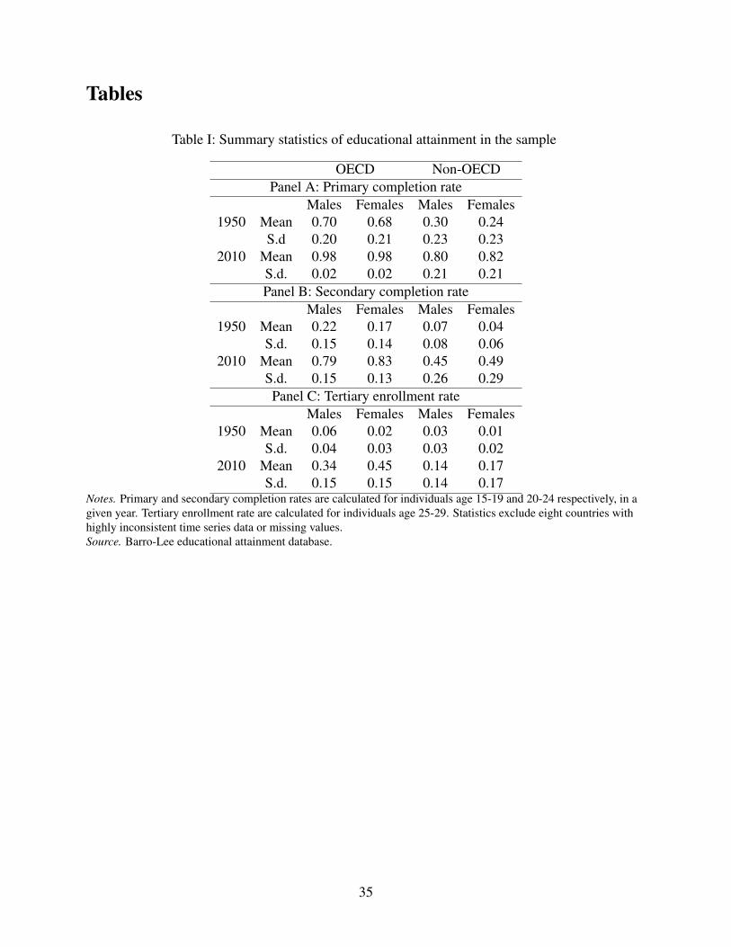
Tables

Table I: Summary statistics of educational attainment in the sample

OECD Non-OECDPanel A: Primary completion rate

Males Females Males Females1950 Mean 0.70 0.68 0.30 0.24

S.d 0.20 0.21 0.23 0.232010 Mean 0.98 0.98 0.80 0.82

S.d. 0.02 0.02 0.21 0.21Panel B: Secondary completion rate

Males Females Males Females1950 Mean 0.22 0.17 0.07 0.04

S.d. 0.15 0.14 0.08 0.062010 Mean 0.79 0.83 0.45 0.49

S.d. 0.15 0.13 0.26 0.29Panel C: Tertiary enrollment rate

Males Females Males Females1950 Mean 0.06 0.02 0.03 0.01

S.d. 0.04 0.03 0.03 0.022010 Mean 0.34 0.45 0.14 0.17

S.d. 0.15 0.15 0.14 0.17Notes. Primary and secondary completion rates are calculated for individuals age 15-19 and 20-24 respectively, in agiven year. Tertiary enrollment rate are calculated for individuals age 25-29. Statistics exclude eight countries withhighly inconsistent time series data or missing values.Source. Barro-Lee educational attainment database.

35

Table II: Share of countries that experienced the gender gap reversal in educational attainment

Primary Secondary TertiaryCompletion Completion Enrollment1950 2010 1950 2010 1950 2010 N

Advanced economies 0.38 0.46 0.21 0.92 0.00 0.96 24East Asia and the Pacific 0.05 0.74 0.00 0.63 0.05 0.68 19Europe and Central Asia 0.50 0.75 0.00 0.85 0.10 0.90 20Latin America and the Caribbean 0.54 0.83 0.12 0.83 0.08 1.00 22Middle East and North Africa 0.06 0.50 0.00 0.88 0.06 0.81 18South Asia 0.00 0.57 0.00 0.42 0.00 0.43 7Sub-Saharan Africa 0.24 0.59 0.06 0.38 0.17 0.31 28

OECD 0.42 0.53 0.14 0.89 0.00 0.94 36Non-OECD 0.25 0.63 0.05 0.65 0.11 0.66 102

All countries 0.29 0.64 0.06 0.71 0.08 0.73 138Notes. The gender gap reversal in educational attainment is defined to occur when the enrollment/completion rate offemales for a given level of education is higher than that of males. Primary and secondary completion rates arecalculated for individuals age 15-19 and 20-24 respectively, in a given year. Tertiary enrollment rates are calculatedfor individuals age 25-29. Statistics exclude eight countries with highly inconsistent time series data or missingvalues.Source. Barro-Lee educational attainment database.

36

Table III: Three hypotheses for the gender gap reversal in education

Corresponding model assumption

Hypothe-sis

Mean of z Variance of z z (or, equivalently, b)

Tail hy-pothesis

- Gender-specific V ar[zm]and V ar[zf ]

-

MBH - - Gender-specific zf and zm (or, equivalently,gender-specific bf and bm)

MPH Gender-specific E[zf ]and E[zm]

- -

Notes. z denotes the scholastic performance of individuals, whose distribution can vary between genders in ourframework. z, which can vary between genders, denotes the lower bound of scholastic performance such thatindividuals enroll into a given level of schooling s.

37

Table IV: Female-to-male ratio in educational attainment, top and bottom 5 countries, 2010

Highest female-to-male ratio Lowest female-to-male ratioTertiary enrollment

Saudi Arabia 2.42 Central African Republic 0.12Slovenia 2.29 Benin 0.16

Dominican Republic 2.17 Afghanistan 0.24Kazakhstan 2.02 Gambia 0.36

Uruguay 2.01 Myanmar 0.36Secondary completion

Nepal 1.90 Congo 0.35Bangladesh 1.79 Afghanistan 0.40Zimbabwe 1.72 Gambia 0.42

Sudan 1.58 Central African Republic 0.47Tanzania 1.53 Democratic Republic of the Congo 0.50

Primary completionMalawi 1.94 Afghanistan 0.63Lesotho 1.85 DR of the Congo 0.73Namibia 1.70 Niger 0.76Myanmar 1.53 Pakistan 0.82

Mali 1.43 Sierra Leone 0.82Notes. The female-to-male ratio is calculated as the enrollment/completion rate of females divided by theenrollment/completion rate of males for a given level of education. Primary and secondary completion rates arecalculated for individuals age 15-19 and 20-24 respectively, in a given year. Tertiary enrollment rates are calculatedfor individuals age 25-29. The ranking excludes countries with highly inconsistent time series and missing values,countries with a female-to-male ratio above 4, and countries with a male or female population under 10,000 for thecorresponding age group.Source. Barro-Lee educational attainment database.

38

Table V: Female-to-male ratio in educational attainment, top and bottom changers between 1950and 2010

Largest increase in ratio Largest decrease in ratioTertiary enrollment

Saudi Arabia 2.26 Central African Republic -0.87Slovenia 1.94 Morocco -0.57

Kazakhstan 1.63 Uganda -0.48Venezuela 1.50 Cambodia -0.35

Croatia 1.47 Niger -0.28Secondary completion

Nepal 1.84 United Kingdom -0.22Bangladesh 1.71 Congo -0.18

Tanzania 1.31 Gambia -0.17Sudan 1.30 Canada -0.13Tunisia 1.29 USA -0.13

Primary completionMalawi 1.69 Mauritania -0.86Uganda 1.06 Dominican Republic -0.62Tanzania 1.00 Norway -0.51

Cambodia 0.97 Bostwana -0.50Egypt 0.90 Russia -0.47

Notes. The female-to-male ratio is calculated as the enrollment/completion rate of females divided by theenrollment/completion rate of males for a given level of education. Primary and secondary completion rates arecalculated for individuals age 15-19 and 20-24 respectively, in a given year. Tertiary enrollment rates are calculatedfor individuals age 25-29. The ranking excludes countries with highly inconsistent time series and missing values,countries with a female-to-male ratio above 4, and countries with a male or female population under 10,000 for thecorresponding age group.Source. Barro-Lee educational attainment database.

39

Table VI: Model estimates of the tail and mean hypotheses parameters, baseline country sample

Main sample Constrained sample

Tail Mean performance Both Tail Mean performance Both GDP & Bothhypothesis hypothesis hypotheses hypothesis hypothesis hypotheses hypotheses

(1) (2) (3) (4) (5) (6) (7)Tertiary enrollmentMale mean (µm) -0.111*** (0.026) 0.540*** (0.010) 0.229*** (0.022) -0.134*** (0.033) 0.588*** (0.016) 0.192*** (0.024) 0.243*** (0.017)Female mean shift per period (µf ) 0.039*** (0.001) 0.029*** (0.002) 0.043*** (0.002) 0.028*** (0.003) 0.026*** (0.004)Male SD (σm) 1.237*** (0.015) 1.142*** (0.010) 1.246*** (0.019) 1.169*** (0.014) 1.166*** (0.009)δ(GDP ) 0.013*** (0.005)R

2 0.47 0.46 0.52 0.5 0.48 0.56 0.57N 1,274 1,274 1,274 715 715 715 715

Secondary completionMale mean (µm) 0.134*** (0.018) 0.465*** (0.034) 0.182*** (0.024) 0.076*** (0.022) 0.554*** (0.014) 0.210*** (0.026) 0.366*** (0.019)Female mean shift per period (µf ) 0.022*** (0.005) 0.0064** (0.0030) 0.032*** (0.002) 0.015*** (0.003) 0.012*** (0.003)Male SD (σm) 1.171*** (0.015) 1.156*** (0.014) 1.213*** (0.016) 1.186*** (0.013) 1.116*** (0.010)δ(GDP ) 0.017*** (0.002)R

2 0.51 0.45 0.51 0.53 0.45 0.53 0.54N 1,274 1,274 1,274 924 924 924 924Notes. ***: significant at the 1% level, **: significant at the 5% level, *: significant at the 10% level. Standard errors are bootstrapped with 1000 repetitions and reported inparentheses. The null hypothesis for σm is σm = 1. The first three columns are estimated with equations (7), (8) and (9), respectively.

40

Table VII: Model estimates of the tail and mean hypotheses parameters, expanded country sample

Main sample Constrained sample

Tail Mean performance Both Tail Mean performance Both GDP & Bothhypothesis hypothesis hypotheses hypothesis hypothesis hypotheses hypotheses

(1) (2) (3) (4) (5) (6) (7)Tertiary enrollmentMale mean (µm) -0.024 (0.024) 0.492*** (0.009) 0.194*** (0.019) -0.102*** (0.033) 0.553*** (0.012) 0.165*** (0.022) 0.277*** (0.018)Female mean shift per period (µf ) 0.031*** (0.001) 0.020*** (0.002) 0.036*** (0.002) 0.024*** (0.003) 0.019*** (0.004)Male SD (σm) 1.180*** (0.014) 1.125*** (0.009) 1.223*** (0.018) 1.168*** (0.013) 1.133*** (0.012)δ(GDP ) 0.023*** (0.005)R

2 0.36 0.35 0.39 0.43 0.38 0.46 0.47N 1,469 1,469 1,469 825 825 825 825

Secondary completionMale mean (µm) 0.118*** (0.019) 0.462*** (0.026) 0.182*** (0.021) 0.070*** (0.023) 0.546*** (0.014) 0.228*** (0.028) 0.371*** (0.019)Female mean shift per period (µf ) 0.023*** (0.004) 0.008*** (0.003) 0.032*** (0.002) 0.016*** (0.003) 0.013*** (0.003)Male SD (σm) 1.167 (0.013) 1.149*** (0.013) 1.210*** (0.017) 1.174*** (0.012) 1.109*** (0.01)δ(GDP ) 0.018*** (0.002)R

2 0.50 0.44 0.50 0.51 0.43 0.51 0.52N 1,469 1,469 1,469 957 957 957 957Notes. ***: significant at the 1% level, **: significant at the 5% level, *: significant at the 10% level. Standard errors are bootstrapped with 1000 repetitions and reported inparentheses. The null hypothesis for σm is σm = 1. The sample includes The sample includes the baseline sample of countries and expands that sample with countries withinconsistent data. The first three columns are estimated with equations (7), (8) and (9), respectively.

41

Table VIII: Model estimates of the tail and mean hypotheses parameters, OECD countries

Main sample Constrained sample

Tail Mean performance Both Tail Mean performance Both GDP & Bothhypothesis hypothesis hypotheses hypothesis hypothesis hypotheses hypotheses

(1) (2) (3) (4) (5) (6) (7)Tertiary enrollmentMale mean (µm) -0.291*** (0.059) 0.548*** (0.027) 0.354*** (0.088) -0.206*** (0.051) 0.608*** (0.023) 0.441*** (0.129) 0.324*** (0.026)Female mean shift per period (µf ) 0.060*** (0.005) 0.051*** (0.006) 0.064*** (0.003) 0.054*** (0.007) 0.048*** (0.007)Male SD (σm) 1.391*** (0.032) 1.109*** (0.036) 1.331*** (0.030) 1.086** (0.047) 1.142*** (0.017)δ(GDP ) -0.001 (0.012)N 416 416 416 275 275 275 275R

2 0.53 0.63 0.65 0.46 0.57 0.58 0.58

Secondary completionMale mean (µm) 0.085** (0.042) 0.331*** (0.063) 0.309 (0.026) 0.060 (0.046) 0.368*** (0.036) 0.308*** (0.029) 0.251*** (0.030)Female mean shift per period (µf ) 0.038*** (0.010) 0.035*** (0.004) 0.040*** (0.005) 0.034*** (0.005) 0.021*** (0.007)Male SD (σm) 1.125*** (0.033) 1.016 (0.021) 1.133*** (0.036) 1.038 (0.029) 1.062*** (0.024)δ(GDP ) 0.003 (0.007)R

2 0.32 0.38 0.38 0.26 0.31 0.32 0.32N 416 416 416 275 275 275 275Notes. ***: significant at the 1% level, **: significant at the 5% level, *: significant at the 10% level. Standard errors are bootstrapped with 1000 repetitions and reported inparentheses. The null hypothesis for σm is σm = 1. The sample includes only OECD countries within the baseline sample of countries. The first three columns are estimatedwith equations (7), (8) and (9), respectively.

42

Table IX: Model estimates of the tail and mean hypothesis parameters, Non-OECD countries

Main sample Constrained sample

Tail Mean performance Both Tail Mean performance Both GDP & Bothhypothesis hypothesis hypotheses hypothesis hypothesis hypotheses hypotheses

(1) (2) (3) (4) (5) (6) (7)Tertiary enrollmentMale mean (µm) -0.086** (0.033) 0.539*** (0.013) 0.189*** (0.023) -0.142*** (0.042) 0.604*** (0.019) 0.224*** (0.027) 0.285*** (0.034)Female mean shift per period (µf ) 0.034*** (0.002) 0.023*** (0.002) 0.040*** (0.002) 0.028*** (0.003) 0.022*** (0.005)Male SD (σm) 1.223*** (0.018) 1.148*** (0.009) 1.245*** (0.023) 1.158*** (0.012) 1.143*** (0.012)δ(GDP ) 0.024** (0.010)R

2 0.22 0.17 0.35 0.25 0.10 0.36 0.44N 858 858 858 440 440 440 440

Secondary completionMale mean (µm) 0.173*** (0.026) 0.501*** (0.015) 0.247*** (0.025) 0.093*** (0.029) 0.606*** (0.016) 0.240*** (0.027) 0.381*** (0.021)Female mean shift per period (µf ) 0.023*** (0.002) 0.009*** (0.003) 0.035*** (0.002) 0.015*** (0.003) 0.010*** (0.004)Male SD (σm) 1.154*** (0.017) 1.131*** (0.015) 1.207*** (0.02) 1.170*** (0.014) 1.112*** (0.013)δ(GDP ) 0.022*** (0.004)R

2 0.49 0.46 0.49 0.48 0.44 0.50 0.51N 858 858 858 649 649 649 649Notes. ***: significant at the 1% level, **: significant at the 5% level, *: significant at the 10% level. Standard errors are bootstrapped with 1000 repetitions and reportedin parentheses. The null hypothesis for σm is σm = 1. The sample includes only non-OECD countries within the baseline sample of countries. The first three columns areestimated with equations (7), (8) and (9), respectively.

43

Figures

Figure I: The Gender Gap Reversal in Educational Attainment

0.0

0.5

1.0

1.5

1960 1980 2000Cohort

Fem

ale−

to−m

ale

ratio

of t

ertia

ry e

nrol

lmen

t

Panel A: Tertiary enrollment

0.0

0.5

1.0

1.5

1960 1980 2000Cohort

Fem

ale−

to−m

ale

ratio

of s

econ

dary

com

plet

ers

Panel B: Secondary completers

0.0

0.5

1.0

1.5

1960 1980 2000Cohort

Fem

ale−

to−m

ale

ratio

of p

rimar

y co

mpl

eter

s

Panel C: Primary completers

Advanced EconomiesEast Asia and the Pacific

Europe and Central AsiaLatin America and the Caribbean

Middle East and North AfricaSouth Asia

Sub−Saharan Africa

Notes. The black line represents the unweighted average for all countries in the sample. Averages are unweightedby country size. In each panel, eight countries were dropped for having highly inconsistent time series or missingobservations.Source. Barro-Lee educational attainment database.

44

Figure II: The ratio of male variance to female variance in test scores in reading (top panel) and mathematics (bottom panel)

Source. Project for International Student Assessment (PISA) 2015.

45

Figure III: Three Hypotheses for the Gender Gap Reversal in Educational Attainment

x1

Panel A: Tail dynamics hypothesis

MalesFemales

z

Academic aptitude, z

Gender−specific and staticdistributions

Dynamic threshold

x1

Panel B: Mean benefits hypothesis (MBH)

MalesFemales

zfzm

Academic aptitude, z

Static distributions

Gender−specific anddynamic threshold

Panel C: Mean performance hypothesis (MPH)

MalesFemales

z

Academic aptitude, z

Gender−specific anddynamic mean

Dynamic threshold

Notes. Panel A: z is the threshold of scholastic performance above which individuals attain a level of schooling ofschooling of at least s, such as tertiary education. The grey arrow indicates a decrease in z over time. Panel B:The grey arrows indicate a faster decrease of zf relative to zm, the female and male-specific scholastic performancethresholds, over time. The distribution of scholastic performance by gender are overlapping as they are identicalunder the mean benefits hypothesis. Panel C: The arrow pointing to the right indicates an increase in mean scholasticperformance of females, µf , relative to males over time as z decreases over time.

46

Figure IV: Distribution Functions of scholastic performance by Gender under the TailHypothesis: Illustration

x1

Panel A: Probability Density Function (PDF) fm(z)

ff(z)

z

Panel B: CCDF

Academic aptitude, zGm(z)Gf(z)

=1

Gm(z)Gf(z)(Gm(z) +Gf(z))/2

Notes. Panel A: The two curves show the probability density functions (pdf) of scholastic performance, z, amongmales (full line) and females (dashed line), with σ2

m>σ2f under the tail dynamics hypothesis and z being normally

distributed. Panel B: The two curves show the complementary cumulative distribution function (ccdf), resulting fromthe integration from +∞ to z of fzf (z) and fzm(z). The grey arrow indicates a decrease in z. The gender gap reversalin educational attainment occurs when the ratio of the two CCDFs reaches 1.

47

Figure V: Relationship between the share of individuals that attain a given level of schooling andthe female-to-male ratio under the tail Hypothesis: Illustration

0 0.5 1

0.5

1

1− Fm(z) + Ff(z)

2

1 − Ff(z)

1 − Fm(z)

Notes. The x-axis reports the share of individuals that attain a level of schooling of at least s. The y-axis measures thefemale-to-male ratio among individuals that attain a level of schooling of at least s. The gender gap reversal occurswhen the female-to-male ratio crosses y=1.

48

Figure VI: Model fit under the tail and mean hypotheses, baseline country sample

●●●●● ●●

●●●

●●●

●

●●

●●

●●

●●

●

●

●

●

●●

●●●

●●

●

●

●

●

●

●

●

●●

●●

●●

●

●●

●●

●●●

●●

●●●●

●●

●

●

●●

●●

●

●

●

●●

●

●● ●

●

●●

●●●

●

● ●

●

●

●

●

●●●

●

●

●

●

●

●

●

●●●

●●●●●●●●●

●●

●

●

●●

●●

●●

●

●●

●●

●

●

●●●●●

●

●

● ●

● ●●

●

●

●

●

●●

●

●

●

●

●●

●

●

●●

● ●

●

●

●

●

●

●

●

●

●

●

●

●

●●●●●●●●

●

●● ●

●●

●●

●

●

● ●

●●

●●

●●

●●●●●

●

●

●

●

●●

●

● ●

●

●●

● ● ●

●

●

●

●●

●●

●●

●

●● ●

●

●

●●

●●

●

●

●● ●

●

●●

●

●

●●

●●

●

●

●

●●

●

●

●

●●●●

●●●●

●

●

●

●

●

●●

●

●● ●● ●

●

●●

●

●

●●●●●●

●●●

●

●●

●

●

●●

●●

●●

●●

●

●●

●

●●●

●

●

●

●

●

●

●

●

●

●

●

●

●

●

● ●

● ●

●

●●

●

●

●●

● ●

●●

●●

●

●

●

●

●●●

●

●

●

●

●●●

●●

●

●●●

●

●

●

●●

● ●

●

●

●

●●●

●●

●

●●

●

●●

●

●●●

●

●

●●

●●

●

●

●

●

●

●●

●●

●●

●●

● ●

● ●

●●

●●●●

●

●● ●

●

●

●

●

●

●

●

●

●

●

●●

● ●

●●

●●

●

●

●

●

●

●● ●

●●

●

●●

●●

●●●●●●

●

●● ●●●

●●●

●●

● ●

●

●●

●●●

●

●●

●

●●

●

●

●●

●

●●

● ●● ●

●

●

●

●

●

●

●

●●

●

●

●

●●●

●

●

●

●

●

●●●

●

●●

●●

●●

●

●

●●●

●●

●●

●● ● ●

● ●

●

●●

●

●

●●

●●

●

●

●

●

●●●●

● ●

●●

●

●●

●

●

●●

●●

●

●

●●

●●●

●

●●●

●●●

●●

●●

●

●

●

●

●

●●

●

●

●

●

●

●●

●

●

●

●

●●

●●

●

●

●

●

●

●●

●

●●●

●●

●

●

●●

●

●

●

●

●

●●

●●

●●

●●

●

●

●●

●●●

● ●

●

●

●

●

●

●●

●

●

●

●

●●

●●

●●

●

●

●

●

●

●●

●

●●●

●●

●●

●

●

●

●●

●●

●●

●●

●●

●

●

●

●

●

●●

●●

●

●

●

●●

●

●

●●

●●

●●

●●

●

●

●

●

●●●●●●●●

●●●

●●

●

●●

●●

●●

●●

●

●

●

●

●

●●

●●

●●

●●

●

●● ●

●

●●

●

●

●

●

●

●●

●

●

●●●●

●●●

●

●●

●

●

●

●●●

●●●●

●●●●

●

●

●

●●

●●

●

●

●●

●

●

●

●

●●

●●

●

●

●

●

●

●● ●

●

● ●● ●

●

●

●

●

●●

●

●

●

●●●

●●

●

●

● ●

●

●●

●

●●●

●●●●

●

●

●

●

●

●

●●

● ●

●●

●●

●

●● ●

●●●●

●

●

● ●●

●

●

●

●

●● ●● ●

●

●

●

●

●

●

●

●

●●

●●

●●

●●●●

●

●

●

●●●

●

●●

●

●●

●

●

●●

●●●

●●

●●

●

●

● ●

●

●

●

●●●

●

●

●

● ●

●

●

●●

●●●●●

●

●

●●●

●

●

●

●●●

●●

●

●

●

●● ●

●

●

●

●●

●●

● ●

●

● ●

● ●

●

●

●

●

● ●

●

●●

●

●

●

●

●

●

●●

●

●

●

●

●

●

●

●●

●

●●●

●●

● ●

●

●

● ●

●

●

●● ●●

●

●

● ●

●

●

●

● ●

●

●

● ●●

●●

●●

●

●

●

●

●●

●

●

●

●●●●●●

●●

●

●

●

●

●

● ●

●

● ●

●●

●

●

●●

●●

●●

●

●●●

●

●

● ●●●●●

●●

●●

●

●

●

●

●●●●●

●●

●●

●

●

●

●

●

●

●

●

●

● ●

●

●

●

●●

●●●

●

●●

●

●●

●

●

●

●●●●

●

●

●●

●

●●

●

●

●●

●●

●●

● ●

●

●

●

●

●

●●

●

●

●●

●

●

●●

●

●

●●

●●

●

●

●●

●

●

●

●

●●

●●

●●

●

●

●

●●

●

●●

●●

●

●

●

●

●

●●●

●

●●

●●●●

●●

●

●

●

●

●

●

●●

●●

●

●

●

●

●

●

●

●

●●●

●

●●●

● ● ●

●

●

●

●

●●

●●

●

●

●

●

●

●

●

●

●●

●

●

●

●● ●

●

●

●

● ●

●

●

●●●

●●●●

●

●●

●

●

●●

●●

● ●

●

●

●

●

●

●

●●●

●●

●●

●●

●●

●●

●●

●●

●●●

●

● ●

●

●

●

●

●

●

●●●●

●

●●

●

●

●

●●

●●

●●

●

●●

● ●●

●

●

●●

● ●

●

●

●

●

●

●●

●●●

●●

●●

●●

●●●

●

●●

●●

● ●

●●

●

●

●

●

●

●●

●

●●

● ●

●●

●●

● ●

●

●●

●●

● ●

●●

●

●

●

●

●●●●●

●●

●●●

● ●

●

●●●

●●

●●

●

●

●●●

●

0.0

0.5

1.0

1.5

2.0

0.00 0.25 0.50 0.75 1.00

Enrollment rate

Sex

ratio

in te

rtiar

y en

rollm

ent

Tertiary enrollment

●●●● ●●

●●

●●

●

●

●

●●

●●

●●

● ●

●

●●

● ●

●

●

●

●

●●

●

●●

●

●

●

●●

●

● ●

●●

●

●

●●● ●

●

● ●●●

●●●●●

●

●●

●

●● ●

● ● ● ●● ●●●●

●

●●

●●

●

●●

●●

● ●●●

●● ●●●

●

●

●

●

●

●

●

●

●●

●

●

●●

●● ● ●

●●●

●●●●●●

●●

●

●● ●

●

● ●●●●

●●

●

● ●

●●●

●●●

●

●

●

●

●

●

●●●●●

●

●●

●

●

●

●

●

●

●● ●

●

● ●

●

●●

●●

●●

●● ●

●●

●●

●●

●●

●

●●

●

●

●●

●●

●●

●●●●

●●

●

●●●

●●

● ●●

●

●●●

●

●

●

●

● ●

●●

●●

●●

●●

●

●●●●

●

●●

●●●●●

●

●

● ●

● ●●

● ● ● ● ●●

●●

●●

●●

●

●

●

●●

●●

●

●●

●

●

●

●

●

●●●

● ●

●

●●●

●●

●

● ●

●● ● ●

●

●

●●●

●●

●

●

●

●●●

● ●

●

●

●● ●

●●●●

●

●

●●

●●●

●●●●

●●

●

●

● ●

●●

●●

●●

● ●● ● ●

●

●

● ●

● ●

●

●

●●●

●

●

●

●

●

●

●

●

●●

● ●●

●

●

●●

●

●

●●

●

●

● ●●●●

●●●●●

●

●●

●

●

●●●

●

● ● ●

●●

● ●●● ●

●

●

●●

●

●

●

● ●

●

●

● ●

● ●

●●

● ● ●

●●

●

●●●

● ●

●

●●

●●

●

●

●

●●

●

●

●

●●

●

●

●

●

●●

●

● ●●

●●●

●●●●

●●● ●

●

●

●

●●●

●●

●

●

●●

●●●

●

●●

●

●

●

● ●

●● ●

●●

●

●●

●

●

●●

●

●●

● ●●●

●

●●

●●●●●●

●

●●●

●

●

●

●

●

●

●● ●

●●

● ●

●●●

●

●

●●

●●

●●

●

●

●

●

●● ●

●

●

●●

●● ●

●

●●

●

●

●●

●●

●

● ●●

●

●●

●●

● ●

●

●

●●●

● ●

●

●

●

●

●

●●

●●

●

●

●●

●●

●

●●

● ●●●●

●

● ●

●●

●

●

●

●

●

●

●

●●

●●

●●

●●

●

●

●

●

●

●

●●

●

●●

●●

●

●

●●

●

●

●

● ●

●

●

●

●

●

●

●

●

●

●

●

●

●

●

●

●

● ●

● ●●

●● ●

●

●

●

●●

●

●●

●● ● ●● ●

●

●●

●●

●

●

●●

● ●●●

●

● ●

● ●

●●

●●

● ●●

● ●

●●

●

●

●●

●

●

● ● ●

● ●

●

●

●

●

●●

●●

●● ●●●

●●

●● ●

●

●●

●

●

●

●

●

●

●

●●

● ● ●●●●●●

●

●

●

●●

●

●

●●

●●

●

●

●

●●

●●

●●

●

●

●

●

●

●

● ●

● ●

●●

●●●●

●

●●

●●

●● ●

●

●

●

●

●●

●

●

●●

●●●● ●

●● ●●

●

●

●●●

●

●

●

●

●●

●

●●

●

●●● ●● ● ●●

●

●

●

●

●

●●●● ●

●

●●

●

●

●

●

●

● ●●

● ●●●

●

●●

●

●●

●●

●●

●● ●●

●

●

●

●

●●

●●●●

●

● ●

●

●

●

●●

●●

●

●●

●

● ●● ●

●

●●●●●●●

●

●●●

●

●

●●

●● ●●

●●

●●

●

●

●

●●

● ●

●

●●

●

●●

●●

●

●

●●

●

●

●

●

●

● ●●

●

●

●●●

●

●

●

●

● ●●

●

●

●

●●

●●

●

●

●●

●

● ●

●

●

●●●●

●● ●●●

●

●

●

●

●●●

●●

●

●

●

●

●

●

●

●

●●● ●

●●

●●

●

●

●

●

●

●●

●●

●●

●

●

●●

●

●

●

●●

●●

●

●

● ●

● ●

●● ●

●● ● ●●

●●●

● ● ●●

●

●

●●

●

●

●

●

●

●

●●

●

●

●

●●

●●

●

●

●●

●

●●

●

●

●●

●

●●

● ●● ●●

●●

●●

●● ●

●

●●

●●

●

●

●●

●

●●

●

●

● ●

●

● ● ● ●

●●

●●

●●

●

●

●

●

●

●●

●

●

●

●

●● ● ● ●

● ●

●

●

●●●

●

●●

●

●

●●

● ●●

●●

●●

●

● ●

●

●●

●

●

●

●●

●

●

●●

● ●●

●●

●●●

●

●

●

●

●

● ●●

●

●

● ● ●

●

●

●

●

●

●● ●● ●

● ●

●

●

●●

● ●●

●●●

●●

●

●

●

●

●

●

●

●

●

●

●

●

●

● ●

● ●●

●●

●●●

● ●

●

●

●

●

●

●

●●●

●● ●●

●●

●●

●●

●●

●

●

●●

●

●●●●●

●●

●●

●

●

●

●

●

●●

● ●●●

●●

●

●

●

●

●

●

●

●

●●

●

● ●●

● ● ●

●

●●●

●●●

●

●

●●

●●

●

●

●

●

●

●

●

●

● ●

●● ●

●●

●

●

●●

●

●● ●● ●

●

● ●

● ●

●●

●

●●

● ●●

●

●●

●

●

●

●

●

●

● ●●

●

●

●●

●●

●●

●

●

●●● ●

●

●

● ●

●

●●

●●

● ● ●●

●

●

●●●●

●●

●

●

●

●

●

●

●●●●

●

●

●

●

●

●

● ●

●

0.0

0.5

1.0

1.5

2.0

0.00 0.25 0.50 0.75 1.00

Completion rate

Sex

ratio

in s

econ

dary

com

plet

ion

Secondary completion

TH: µm = −0.05 , σm = 1.19; MPH: µm = 0.5 , µf = 0.03;Both: µm = 0.19 , µf = 0.02 , σm = 1.13

TH: µm = 0.11 , σm = 1.17; MPH: µm = 0.45 , µf = 0.02;Both: µm = 0.15 , µf = 0.01 , σm = 1.16

●Tail hypo (TH) Mean hypo (MPH) Both hypos (Both)

49

Appendix

A1 Empirical Support for the Model’s Assumptions

A1.1 The Positive Association between scholastic performance and Level of Schooling

The positive relationship between scholastic performance and higher levels of schooling is a key

assumption of the micro model. We test for the validity of this assumption empirically by using

test score data of 10th graders at age 15 for a representative sample of the US population, that

was then followed over time beyond high school. The data is from the Educational Longitudinal

study (ELS) which started in 2002 when individuals where in 10th grade, and allows to link test

scores in 10th grade to whether individuals ever attended post-secondary education in the following

years. Using this data, we estimate a linear probability model of Equation (1), where the dependent

variable is tertiary education attendance, denoted H , which is a function of the latent variable s∗

in the model:

H(s∗) =

1 if s∗ ≥ s

0 if s∗ < s

We therefore estimate b in our model from the binary equivalent of Equation (1) for tertiary edu-

cation, from the regression:

Hj = βzj + εj (10)

Table A1 reports estimated for the empirical relationship between test scores at age 15 and tertiary

education attendance, estimated from the US Educational Longitudinal Survey (ELS). It shows

that test scores at age 15, a proxy for individual scholastic performance z, is a major determinant

of enrollment in tertiary education. The linear probability model coefficient associated with test

scores, i.e the estimate for b in our model, is a positive and highly significant predictor of post-

secondary education enrollment a few years later.21

21Empirically, the propensity to attend tertiary education increases monotonically with test scores rather than shift-ing upward discontinuously beyond a given threshold. Our framework is a simplified version of educational enrollmentdecisions. Empirically, agents certainly enroll into education on the basis of not only individual scholastic performancezj , but also a set of individual circumstances, such as parental income, personal network or taste for schooling that canbe correlated with scholastic performance.

50

Table A1: Model Estimates of the Relationship between scholastic performance and Participationto Tertiary Education, using US Data

Dependent Variable: Dummy forTertiary Education Attendance

(1) (2) (3)

Composite test score 0.449***(0.003)

Reading test score 0.449***(0.003)

Mathematics test score 0.450***(0.003)

Number of observations 12,538 12,538 12,538Notes. ***: significant at the 1% level, **: significant at the5% level, *: significant at the 10% level. Standard errors arereported in parentheses. The regressions are linear probabilitymodels run by ordinary least squares. Regressions do not includean intercept. Test scores were standardized to have a mean of 0and a standard deviation of 1.Source. US Educational Longitudinal Survey (ELS), base year(2002) and 2nd follow-up (2006).

A1.2 The increase in b over time

A increase in the net benefit of education b, leading to an increase in years of schooling over time,

is a key building block of our of our model. To test the validity of this assumption empirically, we

estimate a binary version of Equation 1, where the dependent variable is tertiary education atten-

dance, denoted H . H is observable and is a function of the latent variable s∗ in the model:

H(s∗) =

1 if s∗ ≥ s

0 if s∗ < s

We estimate b, the net benefits to tertiary education in our model, from the linear probability

model:

Hj = βzj + �j,

where β denotes the estimate of b in our model. According to the Barro-Lee data, the gender

gap reversal in participation to tertiary education occurred in the mid 1980s in the US. The data

used for the estimation is from another longitudinal surveys of 10th graders, the High school and

51

Beyond (HS&B), which started in 1980. As for the ELS 2002, this study collects 10th grade test

scores that can be linked to tertiary education attendance a few years later, allowing to estimate

changes in the value of b over the 20-year period in which the reversal occurred.

Table A2 reports our estimates for b in the US in 1980 and 2002 using Equation (1) from our

framework. It shows that the estimated net benefits of tertiary education increased sharply from

1980 to 2002, providing empirical support to the second building block of our model. The null

hypothesis of equality between b1980 and b2002 is strongly rejected by statistical tests. This indicates

that individuals with the same level of scholastic performance are more likely to enroll in higher

education in 2002 than they were in 1980, which is equivalent to higher net benefits of education

in 2002 compared to 1980 in our framework.

Table A2: Model Estimates of the Relationship between scholastic performance and Participationto Tertiary Education in 1980 and 2002, using US Data

Dep. Variable: TertiaryEducation Attendance1980 2002

β 0.278*** 0.450***(0.008) (0.005)

Number of Observations 12,493 12,538Notes. ***: significant at the 1% level, **: significant atthe 5% level, *: significant at the 10% level. Standard er-rors are reported in parentheses. The regressions are linearprobability models run by ordinary least squares. Regres-sions do not include an intercept. Test score are standard-ized to have a mean of 0 and a standard deviation of 1 inthe full sample.Sources. High School and Beyond, base year (1980) and2nd follow-up (1984), US Educational Longitudinal Study,base year (2002) and 2nd follow-up (2006).

This evidence is consistent with a large body of literature showing that returns to education, in

particular returns to tertiary education, have increased over the past decades. Grogger and Eide

(1995) Goldin and Katz (2007) or Acemoglu and Autor (1998) among others provide consistent

evidence of a sharp increase of the college wage premium in the US since the beginning of the

1970s.22 This rise in the college wage premium was also observed in other contexts. Card and22The college wage premium is defined as the wage of college-educated workers relative to the wage of high-school

educated workers.

52

Lemieux (2000) also report an important increase in the wage premium of university graduates

relative to high school graduates in the UK and Canada over the same period.

A1.3 The Negative Relationship between Enrollment Rate and Mean scholastic perfor-

mance of those who Enroll

Given the positive association between individual achievement z and optimal level of schooling s∗

achieved by individuals in our model, a rise in b leads to a simultaneous increase in enrollment, and

to a decrease in z, the scholastic performance threshold for achieving a given level of schooling

s. We do not observe z empirically, but one implication of a decrease in z with no accompanying

increase in the mean of the distribution is a decrease in the mean ability of individuals enrolled,

which can be tested. To do so, we estimate the average verbal test score of individuals that have

attended tertiary education in the US over the period 1975–2010, using data from the General

Social Survey (GSS). From 1974 onwards, the GSS includes a short 10-item multiple choice test

assessing vocabulary knowledge of respondents. A measure of educational attainment in years is

also reported, allowing to identify individuals that attended post-secondary education. We classi-

fied individuals that have completed more than 12 years of schooling as having attended tertiary

education.

Figure A1 depicts the evolution of the average verbal score of post-secondary students relative

to the entire population, from 1975 to 2010. In 1975, the average cognitive score of students at-

tending post-secondary education was 0.60 standard deviation higher than the average cognitive

score of the whole population. This relative difference decreased progressively until 2005 to reach

approximately 0.30 standard deviations in 2010. Consistent with the assumptions of the model,

this suggests that greater access to post-secondary education, an increase in P in our framework,

was accompanied by a decrease in the average test scores of individuals enrolling in tertiary edu-

cation.

53

Figure A1: Empirical Relationship between Enrollment Rate in Tertiary Education and AverageVerbal Score of Participants in Tertiary Education: 1975-2010

●●

●●● ● ●

●

● ● ● ●

● ●

●

●

●●

●

●

● ●●

●●

0.3 0.4 0.5 0.6 0.7

0.0

0.2

0.4

0.6

0.8

1.0

Gross enrollment rate

IQ d

iffer

ence

of c

olle

ge s

tude

nts

and

who

le p

opul

atio

n in

SD

s

●●

●●●●

●

●

●●

●●

●●

●

●

●

● ●●

●●●

●

●

●●

●●● ● ●

●

● ● ● ●

● ●

●●

●

●

●

●

● ●●

● ●

Source. US General Social Survey (1975-2010).Notes. Dots represent point estimates. Vertical lines represent confidence intervals at the 5%-level.

A2 The Mean Dynamics Hypotheses: Supplementary Material

A2.1 The Mean Benefit Hypothesis (MBH)

Goldin, Katz and Kuziemko (2006) or Chiappori, Iyigun and Weiss (2009) suggested that the re-

turns from education, including labor market and marriage market returns, may have risen more

for women over the past decades, which could have driven the gender gap reversal. Both contri-

butions invoke the progressive removal of female career barriers, as a driver of increased returns.

Goldin, Katz and Kuziemko (2006) associate the removal of barriers to female employment to a

54

progressive change in fertility and marriage patterns, driven by the access to reliable contraception

(Goldin and Katz (2002)). The authors posit that this raised females’ expectations regarding future

labor market outcomes, increased labor force participation, and moved female employment out

of traditionally female occupations. In a similar spirit, Chiappori, Iyigun and Weiss (2009) argue

that technological progress has freed women from many domestic tasks, which disproportionally

increased the labor market and marriage market returns of schooling for females. According to

both contributions, the disproportionate increase in the benefits of education for females relative to

males generated the reversal.

We formulate the mean benefits hypothesis in our framework by allowing the net benefits of ed-

ucation b to differ between genders. Let bm and bf denote the net benefits of education for males

and females, where bf and bm are allowed to have different dynamics over time. Gz(.) is assumed

to be identical for males and females. Under the MBH, the optimal level of schooling chosen by

individuals conditional on scholastic performance is gender-specific:

s∗ = z · bg,

or, equivalently, z, is gender specific:

zg =s

bg, (11)

where g = {m; f}, with m standing for males and f for females. Equation 11 states that there

exists gender-specific scholastic performance thresholds such that males and females enroll in a

given level of schooling s, denoted zm and zf respectively. The enrollment rate in a given level of

schooling s reads:

PMBH(zf , zm) ≡

Gz(zm) +Gz(zf )

2, (12)

Under the MBH, a shift from bm > bf to bm < bf over time, or equivalently, from zm < zf to

zm > zf , is a necessary and sufficient condition for the gender gap reversal in education to occur.

The gender ratio among individuals enrolled in a given level of education s is given by:

RMBH(zf , zm) ≡

Gz(zf )

Gz(zm), (13)

55

and:

RMBH

< 1 if zm < zf

RMBH = 1 if zm = zf

RMBH

> 1 if zm > zf .

Using the Barro-Lee data, we parameter values of the model by solving the system of two equations

(12 and 13) and two unknowns {zft , zmt} for each cohort t, where PMBH(zft , zmt) = yt and

RMBH(zft , zmt) = xt.23

A3 Technical Appendix

A3.1 The Tail Hypothesis: Mathematical Proofs of Propositions 1 to 3, Normal Distribu-

tions

Let fzf (z) and fzm(z) denote the probability distribution functions of scholastic performance z for

females and males, respectively. We assume for the sake of the argument that:

zf ∼ N(µf , σ2f)

and

zm ∼ N(µm, σ2m),

where σ2m> σ

2f, according to the tail dynamics hypothesis.

Proof of Proposition 1. The female-to-male ratio RTH(z) tends to zero when the total enrollment

rate PTH(z) tends to zero.

First, it is straightforward to see that limz→∞ PTH(z) =

Gzf (z)+Gzm (z)

2 = 0+02 = 0, where Gz(z) de-

notes the complementary cumulative distribution function (or tail distribution function) of scholas-

tic performance z, defined as� +∞z

fz(z) dz.

23Estimates are available upon request.

56

Let us now study limz→∞ RTH(z). Using the analytical expression of the probability distribution

function of the normal distribution, the ratio RTH(z) can be expressed as:

RTH(z) =

�∞z

1√2πσ2

f

e

(z−µf )2

2σ2f dz

�∞z

1√2πσ2

m

e

(z−µm)2

2σ2m dz

Taking the integrals, one can express the ratio as:

RTH(z) =

12

�1− erf

�z−µf√2σ2

f

��

12

�1− erf

�z−µm√2σ2

m

�� ,

where erf(·) denotes the Gauss error function, defined as erf(z) = 2√π

�z

0 e−t

2dt.

Using the analytical expression of RTH(z), we get:

limz→∞

12

�1− erf

�z−µf√2σ2

f

��

12

�1− erf

�z−µm√2σ2

m

�� = limz→∞

1− (erf [z])

1− (erf [z])=

1− 1

1− 1=

0

0,

where the second to last step follows from the fact that limz→∞ erf(z) = 1.

Using the l’Hôpital rule, we take the derivative of the denominator and the numerator to get the

following expression:

limz→∞

σ2m

σ2f

exp

�(z − µm)2

σ2m

− (z − µf )2

σ2f

�= lim

z→∞

σ2m

σ2f

exp

�(z − µm)2σ2

f

σ2mσ2f

− (z − µf )2σ2m

σ2fσ2m

�

= limz→∞

σ2m

σ2f

exp

�z2σ2f− 2zµmσ

2f+ µ

2mσ2f− z

2σ2m+ 2zµfσ

2m− µ

2fσ2m

σ2mσ2f

�

= limz→∞

σ2m

σ2f

exp

�z

σ2mσ2f

�z{σ2

f− σ

2m}− 2µmσ

2f+ 2µfσ

2m+

µ2mσ2f

z−

µ2fσ2m

z

��= 0,

57

since, by assumption under the tail dynamics hypothesis, σ2m

> σ2f, which are both positive by

definition.

Proof of Proposition 2. The female-to-male ratio RTH(z) tends to one when the total enrollment

rate PTH(z) tends to one.

First, it is straightforward to see that limz→infty PTH(z) =

Gzf (z)+Gzm (z)

2 = 1+12 = 1.

Let us now study the behavior of RTH(z) when z tends to −∞:

limz→−∞

12

�1− erf

�z−µf√2σ2

f

��

12

�1− erf

�z−µm√2σ2

m

�� = limz→−∞

1− (erf [z])

1− (erf [z])=

1 + 1

1 + 1= 1,

where we use the fact that limz→−∞ erf(z) = −1.

Proof of Proposition 3. There exists a value of PTH(z) such that R

TH(z) = 1. This value is

unique and always exists.

Let us now show that given our distributional assumptions, there exists a value of z denoted z∗,

such that the numerator and denominator are of equal value, thus the ratio is one. Again, we invoke

the ratio:

RTH(z) =

12

�1− erf

�z−µf√2σ2

f

��

12

�1− erf

�z−µm√2σ2

m

�� .

Since we know that the error function is monotonously increasing on the whole domain, RTH(z) =

1 when:z−µf√2σ2

f

z−µm√2σ2

m

= 1 ⇔ z − µf

σ2f

=z − µm

σ2m

⇔ z =µmσ

2f− µfσ

2m

σ2f− σ2

m

.

This equation has a unique solution given σ2m

> σ2f. Since the support of E(z) is the whole real

line, there always exists a value of z denoted z∗ such that:

z∗ =

µmσ2f− µfσ

2m

σ2f− σ2

m

.

58

In addition, z∗ is unique given the vector of exogenous parameters {µf , µm, σ2f, σ

2m}.

A3.2 Equivalence of the MPH and MBH hypotheses for uniform distribution within the

intersection of their domains

The MPH in our framework models the gender gap reversal such that females initially have lower

participation rates in education, due to a lower E[z]. Conditional on z, the net benefits of schooling

and the optional level of schooling chosen are identical for both genders: E[s∗f|z] = E[s∗

m|z]. The

MPH and MBH thus differ in the interpretation of the source of the dynamics in the gender mean

differences. They are, in the way they are modeled in our framework, algebraically very similar.

It can be shown that if scholastic performance is normally distributed, they are actually identical

within the intersection of the domains of the two distributions. As a result, the closer the CCDFs

of z are to linear, the more similar the two hypotheses will be in our framework. Here follows

the proof to the claim that the MPH is equivalent to the MBH for uniform distribution within the

intersection of their domains.

MBH: For each time period t, let b ≡ a + c and z ∼ unif(a, b) = unif(a, a + c). Then,

Gz(z) = 1− z−a

b−a= 1− z−a

a+c−a= 1− z−a

c. Also, let (*): zm ≡ z and (**): zf ≡ z + a− af . Now,

for zf , zm ∈ {a, a+ c} ⇔ z + a− af , z ∈ {a, a+ c},

EMBH(zf , zm) =

Gz(zm) +Gz(zf )

2=

1

2

�1− zm − a

(a+ c)− a+ 1− zf − a

(a+ c)− a

�=

1

2

�2− zm + zf − 2a

2c

�

= 1− zm + zf − 2a

4c(∗,∗∗)= 1− 2z − a− af

4cand

RMBH(zf , zm) ≡

Gz(zf )

Gz(zm)= 1− zf − a

(a+ c)− a/1− zm − a

(a+ c)− a=

c

c− zf − a

c/c

c− zm − a

c

59

=c− zf + a

c− zm + a

(∗,∗∗)=

c− z + af

c− z + a

MPH: For z + a− af , z ∈ {a, a+ c},

EMPH(µf , z) =

Gzm(z) +Gzf,t(µf , z)

2=

1

2

�1− z − a

(a+ c)− a+ 1− z − af

(af + c)− af

�

=1

2

�2− 2z − a− af

2c

�= 1− 2z − a− af

4c= E

MBH(zf , zm) and

RMPH(µf , z) ≡

Gzf,t(µf , z)

Gzm(z)= 1− z − af

(af + c)− af/1− z − a

(a+ c)− a=

c

c− z − af

c/c

c− z − a

c

=c− z + af

c− z + a= R

MBH(zf , zm)

Thus, the MBH and MPH are equivalent when scholastic performance is uniformly distributed and

when z + a − af , z ∈ {a, a + c}. The difference between the two hypotheses originates from the

non-linearities in Gz(·).

60