Embed Size (px)
Citation preview

Federal Reserve Bank of Dallas Globalization and Monetary Policy Institute
Working Paper No. 241 http://www.dallasfed.org/assets/documents/institute/wpapers/2015/0241.pdf
What Drives the Global Interest Rate*
Ronald A. Ratti
University of Western Sydney
Joaquin L. Vespignani University of Tasmania
May 2015
Abstract In this paper we study the drivers of global interest rate. Global interest rate is defined as a principal component for the largest developed and developing economies’ discount rates (the US, Japan, China, Euro area and India). A structural global factor-augmented error correction model is estimated. A structural change in the global macroeconomic relationships is found over 2008:09-2008:12, but not pre or post this GFC period. Results indicate that around 46% of movement in central bank interest rates is attributed to changes in global monetary aggregates (15%), oil prices (13%), global output (11%) and global prices (7%). Increases in global interest rates are associated with reductions in global prices and oil prices, increases in trade-weighted value of the US dollar, and eventually to reduce global output. Increases in oil prices are linked with increase in global inflation and global output leading to global interest rate tightening indicated by increases in central bank overnight lending rates. JEL codes: E44, E50, Q43
* Ronald A. Ratti, University of Western Sydney, School of Business, Sydney, Australia. 61-2-9685-9346. [email protected]. Joaquin Vespignani, Tasmanian School of Business and Economics, University of Tasmania Centennial Building, Level 1, Room 114, Private Bag 85, Hobart, Tasmania 7001, Australia. 61-61-3-6226-2802. [email protected]. We thank Denise Osborn, Mardi Dungey and James Morley, as well as seminar and conference participants at Computing in Economics and Finance (2014) and Australasia Econometric Meeting (2014) for commenting in earlier versions of the paper. The views in this paper are those of the authors and do not necessarily reflect the views of the Federal Reserve Bank of Dallas or the Federal Reserve System.

What drives the global interest rate?
1. Introduction
Over the last two decades several important changes have taken place in the global
economy with implications for the interaction of global macroeconomic variables including
central bank discount rates. These developments include a more integrated global economy,
the increasing relative importance of China and India in the global economy, and the different
approaches to monetary policy that have been undertaken by the central banks of the largest
economies following the global financial crisis (GFC). The World Bank estimates (on a
purchasing power parity basis in 2013 US dollars) that the combined GDP of China and India
is about 2/3rds of the combined GDP of the US, Euro area and Japan.1 With the creation of
the European Central Bank and fast economic growth in China and India, the central banks of
the largest 5 economies (the Euro area, U.S., China, Japan and India) have direct
responsibility for stabilizing around 60% of the world economy in recent years.
Policy interest rates set by central banks indicate circumstances within economies
with regard to domestic economic growth and inflation. Bernanke (2015) describes the
Taylor rule (Taylor; 1993) as an important descriptive device by which central bank interest
rate behaviour is captured by variation in inflation relative to target and by output departures
from potential. Hofmann and Bogdanova (2012) have documented that for an extended recent
period central bank policy rates have been below levels implied by the Taylor rule in most
developed and emerging economies. With prolonged economic weakness following the GFC,
1 China and India are likely to be major sources of global economic growth into the future because of demographics, capital accumulation and development. In recent years, cross capital formation and domestic savings rates as percentages of GDP for China and India have averaged over 40% and 30%, respectively (Kónya; 2015). Improvement in investment markets in China and India would raise growth further. Hsieh and Klenow (2009) find that gaps in marginal products of labour and capital across manufacturing plants, imply that equalization of marginal products would raise manufacturing total factor productivity by 30%–50% in China and 40%–60% in India. China and India will also be major consumers of resources. The US Energy Information Agency estimates that China's oil consumption growth was half of the world's oil consumption increase in 2011. The largest oil consuming countries in 2012 are the US, China, Japan and India in that order. India has increased oil consumption by over 50% over 2000-2010. The IEA projects that “China, India, and the Middle East will account for 60% of a 30% increase in global energy demand between now and 2035” (IEA World Energy Outlook 2012: http://www.worldenergyoutlook.org/pressmedia/quotes/12/ ).
2
the central banks of the major developed economies have turned to alternative policies to
expand monetary aggregates and hence stimulate the economy.2
In this paper we seek to answer the question, what drives the global interest rate over
the last fifteen years? The global interest rate reflects the policy interest rates for the main
economies set by their central banks. We believe our paper is the first to examine the
determinants of interest rates at global level. Understanding the behaviour of the interest rate
is crucial to agents making decisions about resource allocation over time in both public and
private spheres. We proposed a structural global factor vector error correction model
(SGFVEC) for this analysis. The methodology builds on the factor augmented vector
autoregressive model (FAVAR) developed by Bernanke et al. (2005).
In the SGFVEC in this paper, structural factors are constructed for central bank
interest rates, real output and CPI across the major developed and developing countries, and
for oil price across various global oil prices. The collective stance of monetary policy actions
by major central banks is in part captured by the level of central bank interest rates at global
level and by the level of global liquidity.3 A factor-augmented error correction dimension to
the SGFVEC model will capture the dynamic of the information provided by many variables
to the analysis of short and long run interaction of global central bank interest rate and
liquidity, global real output, global prices and oil price. It is emphasized that the inclusion of
data on China and India along with that of the major developed economies in the analysis of
the interaction of macro variables at global level is necessary.
2 The recent policies followed by central banks include the following. In the U.S., the Federal Reserve (Fed) undertook its first round of quantitative easing (QE1) in late November 2008, followed by QE2 in November 2010, and QE3 in September 2012. While QE1 was implemented by a one-off purchase of U$ 600 billion in mortgage-back securities and QE2 by a one-off purchase of U$ 600 billion in Treasury securities, QE3 is an ongoing programme purchasing around U$ 85 billion per month in different securities. The European Central Bank (ECB) has been buying covered bonds, a form of corporate debt. The Bank of Japan announced enormous expansions to its asset purchase program in October 2011 and April 2013. The latter event is likely to lead to a doubling of the Japanese money supply in a 2-year period. 3 It is emphasized that this is not the same as the stance of global monetary policy since there is no global central bank. In recent years the effect of global liquidity on the prices of commodities has been emphasized by some researchers. Increases in liquidity raise aggregate demand and thereby increase commodity prices.
3
Global interest rate is found to rise significantly when global output, global prices and
oil prices are increasing. Increases in oil prices are associated with increase in global inflation
and global outputs leading to global interest rate tightening. Consistent with a stronger US
dollar constituting a tightening of global financial conditions, a positive shock to the trade
weighted value of the US dollar results in a significant decline in global interest rates. A
positive shock to central bank discount rates leads to statistically significant and persistent
decline in global M2, reduced CPI and nominal oil price, and to reduced global output.
Positive shocks to global M2, to global CPI, and to global real output are associated with
increases in global oil price. Global liquidity and oil price explain statistically significant
fractions of forecast error variance decomposition in global interest rates. Global money,
global output and global prices are found to be cointegrated. A structural change in the global
macroeconomic relationships is found over 2008:09-2008:12, but not pre versus post GFC.
A brief review of the literature is provided in Section 2. The methodology is described
in Section 3. The data and global variables and factors are discussed in Section 4. The
SGFVEC model is presented in Section 5. The empirical results are presented in Section 6.
The robustness of results to alternative definitions of the variables and different model
specifications is discussed in Section 7. Section 8 concludes.
2 Literature review
Factor methods have become widely used in the literature to examine the co-
movements of country level variables since work by Stock and Watson (1998) and Forni et
al. (2000). Building on Stock and Watson (2002), Bernanke et al. (2005) propose a Factor-
augmented VAR (FAVAR) to identify monetary policy shocks. Mumtaz and Surico (2009)
extend Bernanke et al. (2005) to consider a FAVAR for an open economy. A factor-
augmented approach has been used by Dave et al. (2013) to isolate the bank lending channel
4
in monetary transmission of US monetary policy and by Gilchrist et al. (2009) to assess the
impact of credit market shocks on US activity. Le Bihan and Matheron (2012) use principal
components to filter out sector-specific shocks to examine the connection between stickiness
of prices and the persistence of inflation. Boivin et al. (2009) assume that the connection
between sticky prices and monetary policy can be captured by five common factors estimated
by principal component analysis. Abdallah and Lastrapes (2013) use a FAVAR model to
examine house prices across states in the US.
Global factor variables have been constructed in recent research examining the
determinants of commodity prices. Beckmann et al. (2014b) estimate a structural factor
augmented VAR to examine the links between monetary policies, commodity prices and
share prices with data for the U.S., Euro area, Japan, U.K. and Canada. Juvenal and Petrella
(2014) in an examination of the role of speculation in the oil market, construct a factor for
speculation based on a large number of macroeconomic and financial variables for the G7.
Beckmann et al. (2014a) estimate a Markov switching error correction model based on data
for most of the developed OECD counties finds that liquidity influences commodity price
with effect that change over time. In many of these studies the influence of the major
emerging economies such as China and India on commodity and or oil prices is not usually
considered.
3. Outline of Methodology
In line with the dynamic factor models of Bernanke et al. (2005), Stock and Watson
(2005), Forni and Gambetti (2010), and others, we construct a global factor-augmented error
correction model to examine the relationships between oil prices, global interest rate, global
monetary aggregates, global real output and global CPI. Global factors for interest rates, real
output and CPI are estimated using principal components. A cointegrating vector for global
5
money, global real output and global price level is utilized. A global factor-augmented error
correction model (SGFVEC) is then estimated. The data, variables and various test results are
examined in detail in subsequent sections.
A single individual variable or factor can capture the dynamic of a large amount of
information contained in many variables.4 Facing a large number of variables included in this
study, we use principal component indexes as indicators capturing the effects of global
interest rates, global real output and global price levels by compressing local information on
these variables for the US, Euro area, China, India, and Japan.5
Use of factor analysis for crude oil prices is appropriate for analysis of the behaviour
of the global economy since Brent and West Texas Intermediate (WTI) crude oil price data
have diverged sharply in recent years. Prior to the global financial crisis (GFC) the WTI
crude oil price usually exceeded the Brent by at most a few dollars per barrel, but since the
GFC Brent crude oil price has occasionally topped WTI crude oil price by $28 per barrel. A
global factor for oil price better captures the movement in oil price relevant for the global
economy than do the individual prices for Brent, WTI and Dubai oil. The use of factor
analysis it is also appropriate in modelling the global economy considering the growing
importance of emerging economies in the global economy and world commodity markets.
We favour the global factor approach over other possible ways to model the global
economy, especially over a short period January 1999 to December 2013. The issue of global
variables or global methods have come up in several ways. Use of GDP weights to construct
global variables and conduct analysis with quarterly data rather than use a factor analysis
4 Sims (2002) argues that when deciding policy central banks consider a huge amount of data. An overview of factor-augmented VARs and other models is provided by Koop and Korobilis (2009). Boivin and Ng (2006) caution that expansion of the underlying data could result in factors less helpful for forecasting when idiosyncratic errors are cross-correlated or when a useful factor in a small dataset becomes dominated in a larger dataset. 5 Note that it may be unwise to include more economies that have small global weight, because it might over-represent their impact on global factors estimated by principle component methods. On a GDP PPP basis economies outside the largest five are much smaller individual economies. Activity in the five major economies captures global influences on the global market for oil.
6

with monthly data, would reduce the number of observations considerably, and GDP is not
necessarily the best measure of individual economies influences on oil prices. Factors allow
abstraction of the underlying processes within groups of variables that might not be obtained
by aggregating variables.
We also follow Pesaran et al. (2004) and Dees et al. (2007) GVAR model in the sense
that the interaction of the global economy is considered.6 In the SGFVEC model in this
paper the global factors are treated as endogenous and the interaction of global shocks can be
explicitly examined.
4. Data and global factors
4.1. The Data.
The data are monthly from January 1999 to December 2013. The starting period
coincides with the creation of the European Central Bank and data on CPI and interest rate
for this block is only available from January 1999. Monthly data is used to overcome the
limitation of few observations obtained from quarterly data over a 14 year period. Data are
obtained on the central bank discount rate, monetary aggregate M2, consumer price index,
and industrial production index for each of the five largest economies given by the Euro area,
the US, Japan, China and India. The discount rate is the interest rate charged to banks by the
country’s central bank. 7 Oil prices are given by the Brent, Dubai and West Texas
Intermediate US dollar international indexes for crude oil prices. The trade weighted index
for the US dollar completes the data.8 Data on each country are from the Federal Reserve
Bank of St. Louis (FRED data) and data on oil prices are from the World Bank.
6 Note that for example Dees et al. (2007) the GVAR model combines separate models for each of the many economies linking core variables within each economy with foreign variables using quarterly data. The foreign variables external to a domestic economy are trade-weighted. 7 For the Federal Reserve the federal funds rate is used in place of the discount rate. 8 Major currencies index from the Federal Reserve System of the United State includes: the Euro Area, Canada, Japan, United Kingdom, Switzerland, Australia, and Sweden. Weights are discuss in: http://www.federalreserve.gov/pubs/bulletin/2005/winter05_index.pdf
7
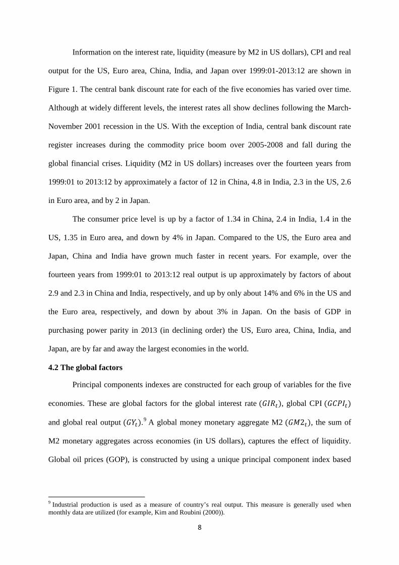
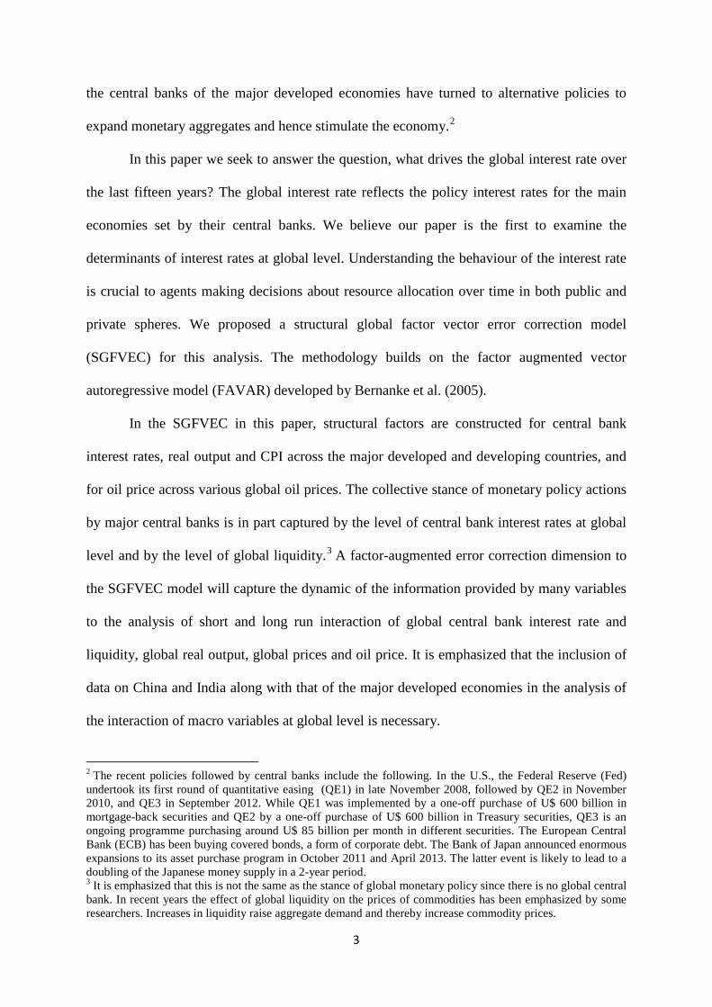
Information on the interest rate, liquidity (measure by M2 in US dollars), CPI and real
output for the US, Euro area, China, India, and Japan over 1999:01-2013:12 are shown in
Figure 1. The central bank discount rate for each of the five economies has varied over time.
Although at widely different levels, the interest rates all show declines following the March-
November 2001 recession in the US. With the exception of India, central bank discount rate
register increases during the commodity price boom over 2005-2008 and fall during the
global financial crises. Liquidity (M2 in US dollars) increases over the fourteen years from
1999:01 to 2013:12 by approximately a factor of 12 in China, 4.8 in India, 2.3 in the US, 2.6
in Euro area, and by 2 in Japan.
The consumer price level is up by a factor of 1.34 in China, 2.4 in India, 1.4 in the
US, 1.35 in Euro area, and down by 4% in Japan. Compared to the US, the Euro area and
Japan, China and India have grown much faster in recent years. For example, over the
fourteen years from 1999:01 to 2013:12 real output is up approximately by factors of about
2.9 and 2.3 in China and India, respectively, and up by only about 14% and 6% in the US and
the Euro area, respectively, and down by about 3% in Japan. On the basis of GDP in
purchasing power parity in 2013 (in declining order) the US, Euro area, China, India, and
Japan, are by far and away the largest economies in the world.
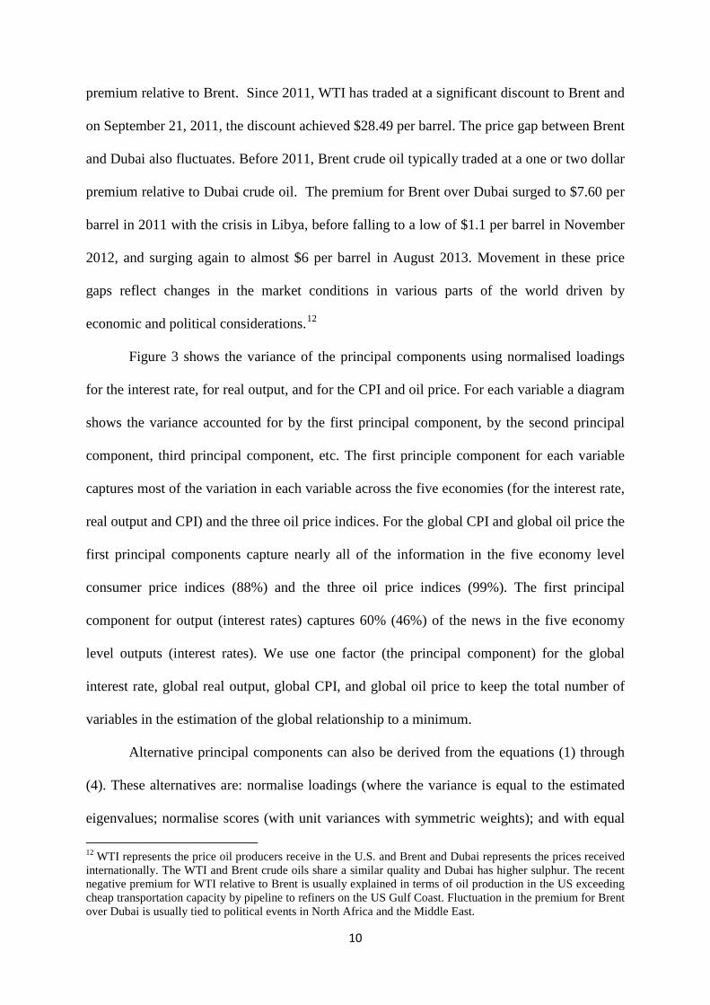
4.2 The global factors
Principal components indexes are constructed for each group of variables for the five
economies. These are global factors for the global interest rate (𝐺𝐺𝐺𝐺𝐺𝐺𝑡𝑡), global CPI (𝐺𝐺𝐺𝐺𝐺𝐺𝐺𝐺𝑡𝑡)
and global real output (𝐺𝐺𝐺𝐺𝑡𝑡).9 A global money monetary aggregate M2 (𝐺𝐺𝐺𝐺2𝑡𝑡), the sum of
M2 monetary aggregates across economies (in US dollars), captures the effect of liquidity.
Global oil prices (GOP), is constructed by using a unique principal component index based
9 Industrial production is used as a measure of country’s real output. This measure is generally used when monthly data are utilized (for example, Kim and Roubini (2000)).
8

on information for the Brent, Dubai and West Texas Intermediate US dollar based
international indexes for crude oil prices.
The indicators of global interest rate, global real output and of global CPI are the
leading principal components for interest rates, real output and CPI (in log-level form for real
output and CPI) of the US, Euro area, China, India, and Japan. These are given by
𝐺𝐺𝐺𝐺𝐺𝐺𝑡𝑡 = [𝐺𝐺𝐺𝐺𝑡𝑡𝐸𝐸𝐸𝐸, 𝐺𝐺𝐺𝐺𝑡𝑡𝑈𝑈𝑈𝑈, 𝐺𝐺𝐺𝐺𝑡𝑡𝐶𝐶ℎ, 𝐺𝐺𝐺𝐺𝑡𝑡𝐽𝐽𝐸𝐸, 𝐺𝐺𝐺𝐺𝑡𝑡𝐼𝐼𝐼𝐼], (1)
𝐺𝐺𝐺𝐺𝑡𝑡 = [𝐺𝐺𝑡𝑡𝐸𝐸𝐸𝐸 ,𝐺𝐺𝑡𝑡𝑈𝑈𝑈𝑈 ,𝐺𝐺𝑡𝑡𝐶𝐶ℎ,𝐺𝐺𝑡𝑡𝐽𝐽𝐸𝐸 ,𝐺𝐺𝑡𝑡𝐼𝐼𝐼𝐼], (2)
𝐺𝐺𝐺𝐺𝐺𝐺𝐺𝐺𝑡𝑡 = [𝐺𝐺𝐺𝐺𝐺𝐺𝑡𝑡𝐸𝐸𝐸𝐸,𝐺𝐺𝐺𝐺𝐺𝐺𝑡𝑡𝑈𝑈𝑈𝑈,𝐺𝐺𝐺𝐺𝐺𝐺𝑡𝑡𝐶𝐶ℎ,𝐺𝐺𝐺𝐺𝐺𝐺𝑡𝑡𝐽𝐽𝐸𝐸,𝐺𝐺𝐺𝐺𝐺𝐺𝑡𝑡𝐼𝐼𝐼𝐼], (3)
where the superscripts Ea, US, Ch, Ja, and In, represent the Euro area, US, China, Japan, and
India, respectively, in equations (1), (2) and (3). In equation (1), 𝐺𝐺𝐺𝐺𝐺𝐺𝑡𝑡 is a vector containing
the discount rate of the central banks of the Euro area, US, China, Japan and India. 10
Equations (2) and (3) are vectors containing the real output and CPI for the same economies,
respectively.11
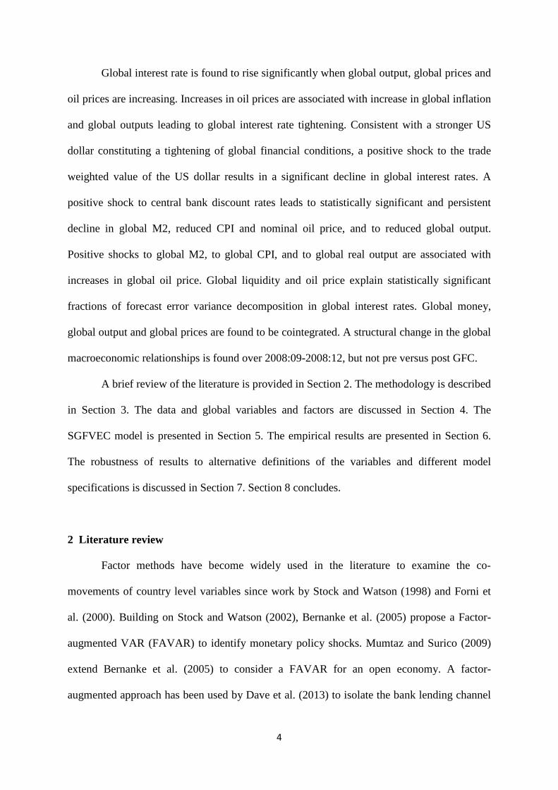
The indicator for global oil prices is the leading principal component of the Dubai,
Brent and West Texas Intermediate oil prices and is given by
𝐺𝐺𝐺𝐺𝐺𝐺𝑡𝑡 = [𝐺𝐺𝐺𝐺𝑡𝑡𝐷𝐷𝐷𝐷𝐷𝐷𝐸𝐸𝐷𝐷,𝐺𝐺𝐺𝐺𝑡𝑡𝑊𝑊𝑊𝑊𝐼𝐼 ,𝐺𝐺𝐺𝐺𝑡𝑡𝐵𝐵𝐵𝐵𝐵𝐵𝐼𝐼𝑡𝑡] (4)
A global factor for oil price better captures movement oil price relevant for the global
economy than the individual prices for Brent, Dubai and WTI oil. US dollar indexes for
Brent, Dubai and WTI crude oil prices are shown in Figure 2. Before the GFC, the WTI and
Brent crude oil prices were within a couple of dollars of each other, with WTI usually at a
10 Structural factors in VAR models to better identify the effects of monetary policy have appeared in a number of contributions (for example, by Belviso and Milani (2006), Laganà (2009) and Kim and Taylor (2012), amongst others), but less so in work on commodity prices. An exception is by Lombardi et al. (2012) examining global commodity cycles in a FAVAR model in which factors represent common trends in metals and food prices. 11 The first principal component for country CPIs to indicate global inflation is similar to Ciccarelli and Mojon (2009) method of identifying global inflation based on price indices for 22 OECD countries and a factor model with fixed coefficients. Within the factor analysis framework, a different approach is taken by Mumtaz and Surico (2012) who derive factors representing global inflation from a panel of 164 inflation indicators for the G7 and three other countries.
9
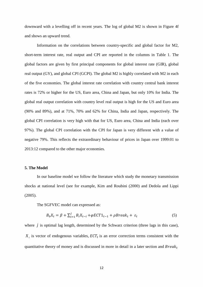
premium relative to Brent. Since 2011, WTI has traded at a significant discount to Brent and
on September 21, 2011, the discount achieved $28.49 per barrel. The price gap between Brent
and Dubai also fluctuates. Before 2011, Brent crude oil typically traded at a one or two dollar
premium relative to Dubai crude oil. The premium for Brent over Dubai surged to $7.60 per
barrel in 2011 with the crisis in Libya, before falling to a low of $1.1 per barrel in November
2012, and surging again to almost $6 per barrel in August 2013. Movement in these price
gaps reflect changes in the market conditions in various parts of the world driven by
economic and political considerations.12
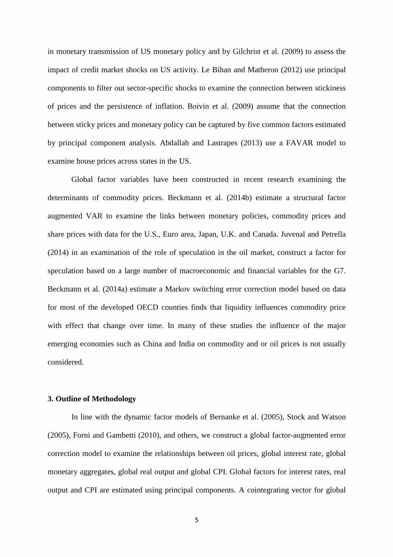
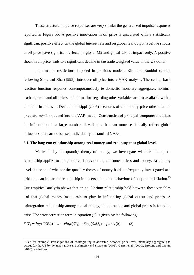
Figure 3 shows the variance of the principal components using normalised loadings
for the interest rate, for real output, and for the CPI and oil price. For each variable a diagram
shows the variance accounted for by the first principal component, by the second principal
component, third principal component, etc. The first principle component for each variable
captures most of the variation in each variable across the five economies (for the interest rate,
real output and CPI) and the three oil price indices. For the global CPI and global oil price the
first principal components capture nearly all of the information in the five economy level
consumer price indices (88%) and the three oil price indices (99%). The first principal
component for output (interest rates) captures 60% (46%) of the news in the five economy
level outputs (interest rates). We use one factor (the principal component) for the global
interest rate, global real output, global CPI, and global oil price to keep the total number of
variables in the estimation of the global relationship to a minimum.
Alternative principal components can also be derived from the equations (1) through
(4). These alternatives are: normalise loadings (where the variance is equal to the estimated
eigenvalues; normalise scores (with unit variances with symmetric weights); and with equal
12 WTI represents the price oil producers receive in the U.S. and Brent and Dubai represents the prices received internationally. The WTI and Brent crude oils share a similar quality and Dubai has higher sulphur. The recent negative premium for WTI relative to Brent is usually explained in terms of oil production in the US exceeding cheap transportation capacity by pipeline to refiners on the US Gulf Coast. Fluctuation in the premium for Brent over Dubai is usually tied to political events in North Africa and the Middle East.
10

weighted scores and loadings. The representation for equal weighted scores and loadings falls
in between those for normalise loadings and normalise scores. In the basic model
constructing principal components we will use normalise loadings and consider use of
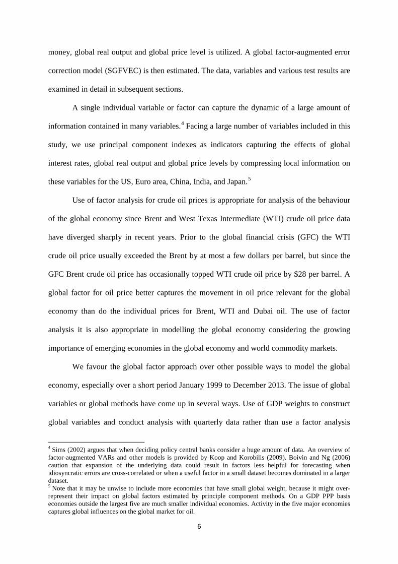
normalise scores in a section on the robustness of results.13 The first principal component for
the global interest rate, to be referred to as 𝐺𝐺𝐺𝐺𝐺𝐺𝑡𝑡 , is drawn in Figure 4a for normalise
loadings, normalise scores, and with equal weighted scores and loadings. It captures the fall
in interest rates at the end of 2008 with the onset of the global financial crisis as well as the
fall in interest rates during and following the 2001 recession in the US. The first principal
component for the CPI indices, 𝐺𝐺𝐺𝐺𝐺𝐺𝐺𝐺𝑡𝑡 , is shown in Figure 4b. In Figure 4 𝐺𝐺𝐺𝐺𝐺𝐺𝐺𝐺𝑡𝑡 slopes
upward. The slight concavity in the curve over 2000-2006 indicates higher CPI over this
period followed by an overall flat rate of inflation in the last half of the sample.
The first principal component for global real output, 𝐺𝐺𝐺𝐺𝑡𝑡, is represented in Figure 4c.
Global real output has an upward trend until the global financial crisis in 2008. There is a
severe correction in 𝐺𝐺𝐺𝐺𝐺𝐺𝑡𝑡 in 2008-2009, reflecting the global financial crisis, with recovery of
global real output to early 2008 levels only in 2011. Global real output also shows a
correction in 2001 coinciding with the March-November 2001 recession in the US. The
principle component for crude oil prices is shown in Figure 4d. Oil price rose sharply from
January 2007 to June 2008. Concurrent with the global financial crisis and the weak global
economy the oil price fell steeply until January 2009 before substantially rebounding over the
next few years. The log of the trade weighted index of the US dollar (USTWI) is shown in
Figure 4e. The trade weighted US dollar peaks in early 2002 and then shows a gradual
13 Note that with normalise loading option more weight is given to variables (countries in this case) with higher standard deviation. With scores options all the variables are given equal weight (by standardising them). The direct implication in this study by choosing normalise loading is that more weight is given to developing economies which generally have higher standard deviation in this sample. This a desirable future of this option considering the views of Hamilton (2009; 2013) and Kilian and Hicks (2013) that for the period of analysis oil prices are largely influenced by the surge in growth in developing economies.
11
downward with a levelling off in recent years. The log of global M2 is shown in Figure 4f
and shows an upward trend.
Information on the correlations between country-specific and global factor for M2,
short-term interest rate, real output and CPI are reported in the columns in Table 1. The
global factors are given by first principal components for global interest rate (GIR), global
real output (GY), and global CPI (GCPI). The global M2 is highly correlated with M2 in each
of the five economies. The global interest rate correlation with country central bank interest
rates is 72% or higher for the US, Euro area, China and Japan, but only 10% for India. The
global real output correlation with country level real output is high for the US and Euro area
(90% and 89%), and at 71%, 70% and 62% for China, India and Japan, respectively. The
global CPI correlation is very high with that for US, Euro area, China and India (each over
97%). The global CPI correlation with the CPI for Japan is very different with a value of
negative 79%. This reflects the extraordinary behaviour of prices in Japan over 1999:01 to
2013:12 compared to the other major economies.
5. The Model
In our baseline model we follow the literature which study the monetary transmission
shocks at national level (see for example, Kim and Roubini (2000) and Dedola and Lippi
(2005).
The SGFVEC model can expressed as:
𝐵𝐵0𝑋𝑋𝑡𝑡 = 𝛽𝛽 + ∑ 𝐵𝐵𝐷𝐷𝑋𝑋𝑡𝑡−𝐷𝐷𝑗𝑗𝐷𝐷=1 +𝜑𝜑𝐸𝐸𝐺𝐺𝐸𝐸1𝑡𝑡−1 + 𝜌𝜌𝐵𝐵𝐵𝐵𝐵𝐵𝐵𝐵𝐵𝐵𝑡𝑡 + 𝜀𝜀𝑡𝑡 (5)
where j is optimal lag length, determined by the Schwarz criterion (three lags in this case),
tX is vector of endogenous variables, 𝐸𝐸𝐺𝐺𝐸𝐸𝑡𝑡 is an error correction terms consistent with the
quantitative theory of money and is discussed in more in detail in a later section and 𝐵𝐵𝐵𝐵𝐵𝐵𝐵𝐵𝐵𝐵𝑡𝑡
12

is a dummy variable which takes the value of 1 from 2008:M9 to 2008:12 and zero otherwise
(as explained in the following section).
The matrix 𝐵𝐵0𝑋𝑋𝑡𝑡 in equation (5) is given by:
𝐵𝐵𝑜𝑜𝑋𝑋𝑡𝑡 =
⎣⎢⎢⎢⎢⎡
1 −𝑏𝑏01 0 0 0 −𝑏𝑏05−𝑏𝑏10 1 −𝑏𝑏12 −𝑏𝑏13 0 0
0 0 1 −𝑏𝑏23 −𝑏𝑏24 00 0 0 1 −𝑏𝑏34 00 0 0 0 1 0
−𝑏𝑏50 −𝑏𝑏51 −𝑏𝑏52 −𝑏𝑏53 −𝑏𝑏54 1 ⎦⎥⎥⎥⎥⎤
⎣⎢⎢⎢⎢⎢⎡ ∆ log(𝐺𝐺𝐺𝐺𝐺𝐺𝑡𝑡) ∆ log(𝐺𝐺𝐺𝐺2𝑡𝑡) ∆ log(𝐺𝐺𝐺𝐺𝐺𝐺𝐺𝐺𝑡𝑡)∆ log(𝐺𝐺𝐺𝐺𝑡𝑡) ∆ log(𝐺𝐺𝐺𝐺𝐺𝐺𝑡𝑡)∆log (𝑈𝑈𝑈𝑈𝐸𝐸𝑈𝑈𝐺𝐺𝑡𝑡)⎦
⎥⎥⎥⎥⎥⎤
(6)
Consistent with Gordon and Leeper (1994), Christiano et al. (1999) , Kim and
Roubini (2000), Sims and Zha (2006) the impact effects of financial shocks on industrial
production and consumer prices are zero, but contemporaneous response to both monetary
aggregates and oil prices. Monetary aggregates M2 respond contemporaneously to the
domestic interest rate, CPI and real output assuming that the real demand for money depends
contemporaneously on the interest rate and real income. The CPI is influenced
contemporaneously by both real output and oil prices, while real output is assumed to be
influenced by oil prices. 14
Oil prices are assumed to be contemporaneously exogenous to all variables in the
model on the ground of information delay. Given the forward looking nature of exchange rate
on asset prices and this variable’s information is available daily, the exchange rate is assumed
to respond contemporaneously to all variables in the model.
The vector 𝑋𝑋𝑡𝑡 is expressed as:
𝑋𝑋𝑡𝑡 = [𝐺𝐺𝐺𝐺𝐺𝐺𝑡𝑡,∆ log(𝐺𝐺𝐺𝐺2𝑡𝑡) , log(𝐺𝐺𝐺𝐺𝐺𝐺𝐺𝐺𝑡𝑡) ,∆ log(𝐺𝐺𝐺𝐺𝑡𝑡),∆ log(𝐺𝐺𝐺𝐺𝐺𝐺𝑡𝑡),∆log (𝑈𝑈𝑈𝑈𝐸𝐸𝑈𝑈𝐺𝐺𝑡𝑡) ], (7)
where the variables are affirmed as the global interest rate (𝐺𝐺𝐺𝐺𝐺𝐺𝑡𝑡), global M2 (𝐺𝐺𝐺𝐺2𝑡𝑡), global
CPI (𝐺𝐺𝐺𝐺𝐺𝐺𝐺𝐺𝑡𝑡) , global output (𝐺𝐺𝐺𝐺𝑡𝑡) , oil price (𝐺𝐺𝐺𝐺𝐺𝐺𝑡𝑡) , and the trade weighted US dollar
exchange rate (𝑈𝑈𝑈𝑈𝐸𝐸𝑈𝑈𝐺𝐺𝑡𝑡). ∆ is the first difference operator.
14 Forni and Gambetti (2010) refer to the assumption that output and consumer prices within a country do not respond contemporaneously to financial variables as a standard identification scheme in the literature.
13
These structural impulse responses are very similar the generalized impulse responses
reported in Figure 5b. A positive innovation in oil price is associated with a statistically
significant positive effect on the global interest rate and on global real output. Positive shocks
to oil price have significant effects on global M2 and global CPI at impact only. A positive
shock in oil price leads to a significant decline in the trade weighted value of the US dollar.
In terms of restrictions imposed in previous models, Kim and Roubini (2000),
following Sims and Zha (1995), introduce oil price into a VAR analysis. The central bank
reaction function responds contemporaneously to domestic monetary aggregates, nominal
exchange rate and oil prices as information regarding other variables are not available within
a month. In line with Dedola and Lippi (2005) measures of commodity price other than oil
price are now introduced into the VAR model. Construction of principal components utilizes
the information in a large number of variables that can more realistically reflect global
influences that cannot be used individually in standard VARs.
5.1. The long run relationship among real money and real output at global level.
Motivated by the quantity theory of money, we investigate whether a long run
relationship applies to the global variables output, consumer prices and money. At country
level the issue of whether the quantity theory of money holds is frequently investigated and
held to be an important relationship in understanding the behaviour of output and inflation.15
Our empirical analysis shows that an equilibrium relationship hold between these variables
and that global money has a role to play in influencing global output and prices. A
cointegration relationship among global money, global output and global prices is found to
exist. The error correction term in equation (1) is given by the following:
𝐸𝐸𝐺𝐺𝐸𝐸𝑡𝑡 = 𝑙𝑙𝑙𝑙𝑙𝑙(𝐺𝐺𝐺𝐺𝐺𝐺𝐺𝐺𝑡𝑡) − 𝛼𝛼 − 𝜃𝜃𝑙𝑙𝑙𝑙𝑙𝑙(𝐺𝐺𝐺𝐺𝑡𝑡) − 𝛿𝛿log (𝐺𝐺𝐺𝐺2𝑡𝑡) + 𝜌𝜌𝑡𝑡 ~ 𝐺𝐺(0) (3)
15 See for example, investigations of cointegrating relationship between price level, monetary aggregate and output for the US by Swanson (1998), Bachmeier and Swanson (2005), Garret et al. (2009), Browne and Cronin (2010), and others.
14
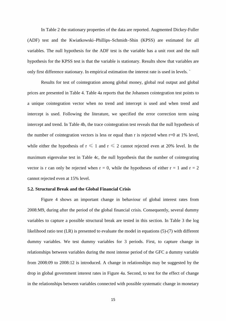
In Table 2 the stationary properties of the data are reported. Augmented Dickey-Fuller
(ADF) test and the Kwiatkowski–Phillips–Schmidt–Shin (KPSS) are estimated for all
variables. The null hypothesis for the ADF test is the variable has a unit root and the null
hypothesis for the KPSS test is that the variable is stationary. Results show that variables are
only first difference stationary. In empirical estimation the interest rate is used in levels. `
Results for test of cointegration among global money, global real output and global
prices are presented in Table 4. Table 4a reports that the Johansen cointegration test points to
a unique cointegration vector when no trend and intercept is used and when trend and
intercept is used. Following the literature, we specified the error correction term using
intercept and trend. In Table 4b, the trace cointegration test reveals that the null hypothesis of
the number of cointegration vectors is less or equal than r is rejected when r=0 at 1% level,
while either the hypothesis of r ≤ 1 and r ≤ 2 cannot rejected even at 20% level. In the
maximum eigenvalue test in Table 4c, the null hypothesis that the number of cointegrating
vector is r can only be rejected when r = 0, while the hypotheses of either r = 1 and r = 2
cannot rejected even at 15% level.
5.2. Structural Break and the Global Financial Crisis
Figure 4 shows an important change in behaviour of global interest rates from
2008:M9, during after the period of the global financial crisis. Consequently, several dummy
variables to capture a possible structural break are tested in this section. In Table 3 the log
likelihood ratio test (LR) is presented to evaluate the model in equations (5)-(7) with different
dummy variables. We test dummy variables for 3 periods. First, to capture change in
relationships between variables during the most intense period of the GFC a dummy variable
from 2008:09 to 2008:12 is introduced. A change in relationships may be suggested by the
drop in global government interest rates in Figure 4a. Second, to test for the effect of change
in the relationships between variables connected with possible systematic change in monetary
15

policy during and after the global financial crises, a dummy variable is introduced from
2009:01 to the end of the sample. A systematic change in monetary policy would be reflected
in quantitative easing in the developed countries discussed earlier. Thirdly, to capture the
effects of both the first two dummy variables, a dummy variable is introduced from 2008:09
to the end of the sample. This dummy variable captures systematic change that immediately
started with the initial shock of the GFC that continues beyond the crisis through to the
present.
Results in Table 3, shows that LR test rejects the null hypothesis at 1% level of no
structural break for the dummy variable from the period 2008:09 to 2008:12 (the chi-square
value is 39.66). The null hypothesis of no structural break for the dummy variables from the
periods 2008:09 to 2013:12 and from 2009:01 to 2013:12 cannot be rejected. In line with
these results we include a dummy variable, value 1 over 2008:09 to 2008:12 and 0 otherwise,
in the model in equations (5) to (7).
6. Empirical Results
The responses of variables in the SGFVEC model (in equations (5), (6) and (7)) to
one-standard deviation structural innovations are shown in Figure 5. The dashed lines
represent a one standard error confidence band around the estimates of the coefficients of the
impulse response functions.16 The first row in Figure 5 shows the response of the global
interest rate to structural innovations in the global interest rate, global M2, global CPI, global
output, oil price, and the trade weighted US dollar exchange rate, in turn. Similarly, the
second, third, fourth, fifth and sixth rows show the response of global M2, global CPI, global
output, oil price, and the trade weighted US dollar exchange rate, respectively, to structural
16 The confidence bands are obtained using Monte Carlo integration as described by Sims (1980), where 5000 draws were used from the asymptotic distribution of the VAR coefficient.
16
innovations in 𝐺𝐺𝐺𝐺𝐺𝐺𝑡𝑡 , ∆ log(𝐺𝐺𝐺𝐺2𝑡𝑡) , ∆log(𝐺𝐺𝐺𝐺𝐺𝐺𝐺𝐺𝑡𝑡) , in ∆log (𝐺𝐺𝐺𝐺𝑡𝑡) , ∆ log(𝐺𝐺𝐺𝐺𝐺𝐺𝑡𝑡) , and
∆log(𝑈𝑈𝑈𝑈𝐸𝐸𝑈𝑈𝐺𝐺𝑡𝑡) in turn.
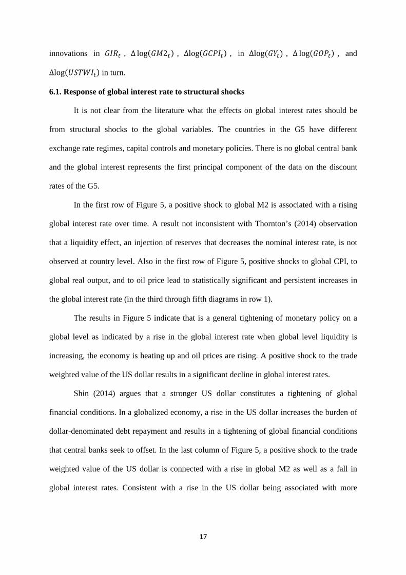
6.1. Response of global interest rate to structural shocks
It is not clear from the literature what the effects on global interest rates should be
from structural shocks to the global variables. The countries in the G5 have different
exchange rate regimes, capital controls and monetary policies. There is no global central bank
and the global interest represents the first principal component of the data on the discount
rates of the G5.
In the first row of Figure 5, a positive shock to global M2 is associated with a rising
global interest rate over time. A result not inconsistent with Thornton’s (2014) observation
that a liquidity effect, an injection of reserves that decreases the nominal interest rate, is not
observed at country level. Also in the first row of Figure 5, positive shocks to global CPI, to
global real output, and to oil price lead to statistically significant and persistent increases in
the global interest rate (in the third through fifth diagrams in row 1).
The results in Figure 5 indicate that is a general tightening of monetary policy on a
global level as indicated by a rise in the global interest rate when global level liquidity is
increasing, the economy is heating up and oil prices are rising. A positive shock to the trade
weighted value of the US dollar results in a significant decline in global interest rates.
Shin (2014) argues that a stronger US dollar constitutes a tightening of global
financial conditions. In a globalized economy, a rise in the US dollar increases the burden of
dollar-denominated debt repayment and results in a tightening of global financial conditions
that central banks seek to offset. In the last column of Figure 5, a positive shock to the trade
weighted value of the US dollar is connected with a rise in global M2 as well as a fall in
global interest rates. Consistent with a rise in the US dollar being associated with more
17

constrictive global financial conditions (for given central bank interest rates) there are
declines in CPI, real output and oil prices for extended periods.
6.2. Response of global variables to structural shock to global interest rate
In the first column of Figure 5, a positive shock to global interest rates leads to
statistically significant and persistent decline in global M2. Monetary tightening at global
level is connected with reduced CPI and nominal oil price, and after a positive bump to
reduced global output. In the second column of Figure 5, a positive shock to global M2 is
linked with increases in CPI and in nominal oil price, and after four months with increased
global output.
6.3. Liquidity and structural shocks
The second column in Figure 5 reports the effects on the global variables of a positive
structural shock to liquidity. Global liquidity significantly impacts global CPI 3 and 4 months
later. The impact on oil price is statistically significant after 3 months and remains so over the
20 month horizon. A positive innovation in global liquidity significantly impacts output over
a 5 to 13 month horizon. The trade weighted value of the US dollar declines with a positive
innovation in global M2 and the effect is immediate and persists over the entire horizon. In
line with results in the literature, increase in global liquidity is associated with global
expansion and rising oil and global consumer prices.
6.4. The oil price and structural shocks
The impulse responses of oil price to global variables are presented in the fifth row of
Figure 5. A negative shock to global interest rates and positive shocks to global M2, to global
CPI, and to global real output, lead to statistically significant and persistent increases in
global oil price (in the first through fourth diagrams). A positive innovation in M2 supports a
higher level of spending with positive effects on nominal oil price. A positive shock in the
global CPI, reflects a negative shock to the real price of oil and an increase in oil price. A
18

positive innovation in global real output indicates a higher level of global real activity with
concomitant increases in the demand for crude oil and an increase in the global oil price.
In the fifth column of Figure 5, a positive innovation in oil price is associated with a
statistically significant positive effect on the global interest rate and on global real output.
Positive shocks to oil price have significant effects on global M2 and global CPI at impact
only. A negative shock in oil price leads to a statistically significant increase in the trade
weighted value of the US dollar.
6.5. Variance decomposition
An important question concerns how much of the variation in global interest rates,
global M2, global price level, global output and oil price is explained by the variables in the
model. Decomposition of the forecast error variance into components provides insight on the
percent contribution of the structural shocks to the variation of GIR, GM2, GCPI, GY and oil
price.
Table 5 panel reports the fraction of forecast error variance decomposition (FEVDs)
of global interest rate set by central banks. Global M2, global output and oil price each make
statistically significant contributions to forecasting the variation in global interest rate over
different time horizons. The contribution of global M2 explains 51.40% of the variation in
global interest rate in the first month. This fraction declines over time and becomes 15.30% at
the 36 month horizon. Oil price does not make a statistically significant contribution to
forecast error variance decomposition of global interest rate in the first 6 months, but does at
and after the 12 month horizon. The contribution of oil price to explaining the variation in
global interest rate rises over time, becoming 10.6% at 12 months and 13.10% at 36 months.
The contribution of global output to explaining the variation in global interest rate also rises
over time and becomes a statistically significant 10.7% at the 24 month horizon. Global CPI
19
and the trade weighted USD dollar do not contribute significantly to explaining variation in
global interest rate.
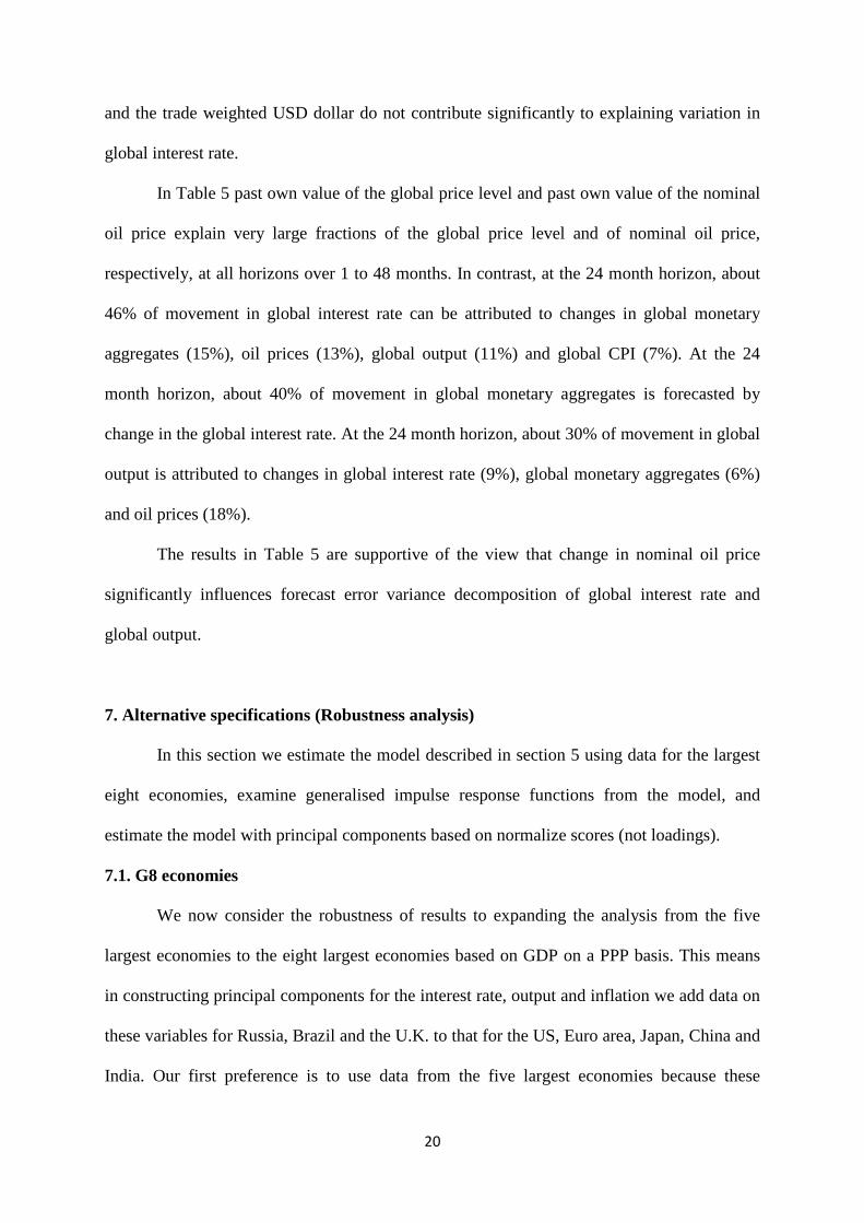
In Table 5 past own value of the global price level and past own value of the nominal
oil price explain very large fractions of the global price level and of nominal oil price,
respectively, at all horizons over 1 to 48 months. In contrast, at the 24 month horizon, about
46% of movement in global interest rate can be attributed to changes in global monetary
aggregates (15%), oil prices (13%), global output (11%) and global CPI (7%). At the 24
month horizon, about 40% of movement in global monetary aggregates is forecasted by
change in the global interest rate. At the 24 month horizon, about 30% of movement in global
output is attributed to changes in global interest rate (9%), global monetary aggregates (6%)
and oil prices (18%).
The results in Table 5 are supportive of the view that change in nominal oil price
significantly influences forecast error variance decomposition of global interest rate and
global output.
7. Alternative specifications (Robustness analysis)
In this section we estimate the model described in section 5 using data for the largest
eight economies, examine generalised impulse response functions from the model, and
estimate the model with principal components based on normalize scores (not loadings).
7.1. G8 economies
We now consider the robustness of results to expanding the analysis from the five
largest economies to the eight largest economies based on GDP on a PPP basis. This means
in constructing principal components for the interest rate, output and inflation we add data on
these variables for Russia, Brazil and the U.K. to that for the US, Euro area, Japan, China and
India. Our first preference is to use data from the five largest economies because these
20

economies are much closer in size than when sixth, seventh and eights economies are
included (Russia, Brazil and the U.K. respectively). 17 However, the major developing
economies taken to be the BRIC countries, Brazil, the Russian Federation, India and China,
have dramatic increases in real income in recent years and their inclusion along with the
largest developed economies in an analysis of global effects of oil prices is a reasonable
robustness analysis. The global measure of M2 will now be the sum of M2 in the largest eight
economies in US dollars.
In Figure 6, the global variables created with principal components for both the group
of five largest economies and the group of eight largest economies are plotted. 18 For
conciseness the group of five largest economies is termed G5 and the group of eight largest
economies is termed G8. The global interest rate (first principal component) based on the G5
is slightly higher (lower) in the first (second) half of the sample than that based on the G8.
However, the movements in both G5 and G8 based global interest rates closely track one
another.
The global CPI based on data for the G8 has steeper slope the global CPI based on
data for the G5. This is due to Brazil and Russia both having had substantial increases in
price levels (compared to the other economies) over 1999-2013. Global output given by the
principal component for output in the G8 has less steep recessions following 2001 (the
recession in the US) and that following the global financial crisis than indicated by the
principal component for output in the G5. M2 for the G8 shows similar pattern to that for the
G5.
The response of variables in the SGFVEC model (in equations (5) and (6)) for G8
variables to one-standard deviation structural innovations are shown in the first rows in
17 Note that the risk of including economies of different sizes may lead to the overrepresentation (weights) of small economies when principal components are used. 18 The G8 economies account for around 70% of world GDP measure by real PPP in US DOLLARS.
21
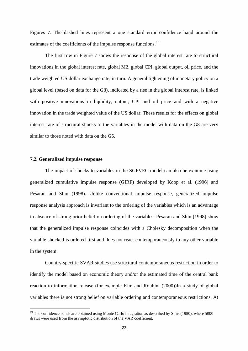
Figures 7. The dashed lines represent a one standard error confidence band around the
estimates of the coefficients of the impulse response functions.19
The first row in Figure 7 shows the response of the global interest rate to structural
innovations in the global interest rate, global M2, global CPI, global output, oil price, and the
trade weighted US dollar exchange rate, in turn. A general tightening of monetary policy on a
global level (based on data for the G8), indicated by a rise in the global interest rate, is linked
with positive innovations in liquidity, output, CPI and oil price and with a negative
innovation in the trade weighted value of the US dollar. These results for the effects on global
interest rate of structural shocks to the variables in the model with data on the G8 are very
similar to those noted with data on the G5.
7.2. Generalized impulse response
The impact of shocks to variables in the SGFVEC model can also be examine using
generalized cumulative impulse response (GIRF) developed by Koop et al. (1996) and
Pesaran and Shin (1998). Unlike conventional impulse response, generalized impulse
response analysis approach is invariant to the ordering of the variables which is an advantage
in absence of strong prior belief on ordering of the variables. Pesaran and Shin (1998) show
that the generalized impulse response coincides with a Cholesky decomposition when the
variable shocked is ordered first and does not react contemporaneously to any other variable
in the system.
Country-specific SVAR studies use structural contemporaneous restriction in order to
identify the model based on economic theory and/or the estimated time of the central bank
reaction to information release (for example Kim and Roubini (2000))In a study of global
variables there is not strong belief on variable ordering and contemporaneous restrictions. At
19 The confidence bands are obtained using Monte Carlo integration as described by Sims (1980), where 5000 draws were used from the asymptotic distribution of the VAR coefficient.
22
the global level, whether global interest rate responds to global CPI is less clear, as the global
variables are composed of several country-specific variables.
We report in the second row of Figure 7 the responses of the global interest rate in the
SGFVEC model in equations (5) and (7) to one standard deviation generalised cumulative
impulse response function in global interest rate, global M2, global CPI, global output, oil
price, and the trade weighted US dollar exchange rate. We are using one standard deviation
generalised cumulative impulse response function following Pesaran and Shin (1998). The
dashed lines represent a one standard error confidence band around the estimates of the
coefficients of the cumulative impulse response functions.20
The results for effects on GIR in the second row of Figure 7 are based on G5
variables. Positive shocks to global M2, to global CPI, to global real output, and to oil price
lead to statistically significant positive effects on the global interest rate that increase over
time. A positive shock to the trade weighted value of the US dollar results in a significant
decline in global interest rates. The results of the generalised cumulative impulse response are
very similar to those from the impulse response results from the structural model in equation
(6), and confirm the finding of a rise in the global interest rate when global level liquidity is
increasing, the economy is growing and oil prices are increasing.
The generalised cumulative impulse response functions of global M2 and oil price to
one standard deviation shocks in the variables in the SGFVEC model are reported in the
second rows of Figures 8 and 9, respectively. The generalised cumulative impulse responses
are very similar to those obtained the impulse response results from the structural model
specified in equation (6).
7.3. Different weights in principal components
20 The confidence bands are obtained using Monte Carlo integration as described by Sims (1980), where 5000 draws were used from the asymptotic distribution of the VAR coefficient.
23
Our baseline model uses principal components with normalise loadings to construct
the variables GIR, GCPI, GY and GOP. In this section we use principal components with
normalise scores to construct these variables. The responses of these variables, constructed
with normalise scores in the SGFVEC model (in equations (5), (6) and (7)), are examined to
one-standard deviation structural innovations in the variables in the model. The cumulative
impulse response function of the global interest rate with normalise scores to one standard
deviation shocks in the variables in the model are reported in the third row of Figure 7.
Results are virtually identical to those obtained in the first row of Figure 5 for our baseline
model using principal components with normalise loadings.
The cumulative impulse response functions of global M2 and oil price to one
standard deviation shocks in the variables in the SGFVEC model using principal components
with normalise scores are reported in the third rows of Figures 8 and 9, respectively. The
impulse responses for GM2 and GOP are very similar to the impulse response results for
these variables reported in Figure 5 for the baseline model using principal components with
normalise loadings.
8. Conclusion
A structural global factor vector error correction model is estimated to examine the
interaction of global interest rates, monetary aggregates, and output and consumer prices and
oil prices at global level. The major economies are taken to be the world's three largest
developed economic blocs (the US, Japan and the Euro area), and the two largest emerging
market economies, China and India, that are increasingly important in shaping the global
economy. Global money, global output and global prices are found to be cointegrated. A
structural change in the global macroeconomic relationships is found over 2008:09-2008:12,
but not pre versus post GFC.
24
It is found that there is statistically significant rise in global interest rates when global
consumer prices and oil prices are increasing. This indicates a general easing of monetary
policy on a global level given economic weakness and falling prices. A positive shock to
global interest rate leads to statistically significant and persistent decline in global M2,
reduced CPI and nominal oil price, and after several months to reduced global output. A
positive shock to the trade weighted value of the US dollar results in a significant decline in
global interest rates. A stronger US dollar constitutes a tightening of global financial
conditions that central banks seek to offset by reducing discount rates. Increases in oil prices
are associated with increase in global inflation and global output leading to global interest
rate tightening.
A negative shock to global interest rates leads to statistically significant and persistent
increases in global oil price. Positive shocks to global M2, to global CPI, and to global real
output are associated with increases in global oil price. These shocks are consistent with
higher levels of global real activity and thus with increases in global oil price. A positive
shock in oil price leads to a significant decline in the trade weighted value of the US dollar.
Global liquidity, global output and oil price explain statistically significant fractions of
forecast error variance decomposition in the principal component for global interest rates, in
amounts given by 15%, 11% and 13%, respectively.
Results are robust to alternative identification schemes in the structural global factor
vector error correction model, to different measurement of global variables, to treatment of
the global financial crisis, and to variation in lag length. Findings suggest that when
considering movement in the global level of central bank interest rates it is necessary to
consider the influence of global variables that reflect developments in the major developing
and developed countries.
25
References
Abdallah, C.S., Lastrapes, W.D., 2013. Evidence on the Relationship between Housing and Consumption in the United States: A State-Level Analysis. Journal of Money, Credit and Banking 45, 559-589. Bachmeier, L.J., Swanson, N.R., 2005. Predicting Inflation: Does The Quantity Theory Help? Economic Inquiry 43, 570-585. Beckmann, J, Belke, A and Czudaj, R., 2014a. Does global liquidity drive commodity prices? Journal of Banking and Finance 48, 224-234. Beckmann, J, Belke, A and Czudaj, R., 2014b. The importance of global shocks for national policymakers-rising challenges for sustainable monetary policies. The World Economy 37, 1101–1127. Belviso, F., Milani, F., 2006. Structural factor-augmented VARs (SFAVARs) and the effects of monetary policy. Topics in Macroeconomics, 6-3, Article number 2. Incorporated in: B.E. Journal of Macroeconomics. Bernanke, B.S., 2015. The Taylor Rule: A benchmark for monetary policy? Ben Bernanke’s Blog. http://www.brookings.edu/blogs/ben-bernanke/posts/2015/04/28-taylor-rule-monetary-policy Bernanke, B., Boivin, J., Eliasz, P.S., 2005. Measuring the Effects of Monetary Policy: A Factor-augmented Vector Autoregressive (FAVAR) Approach. Quarterly Journal of Economics 120, 387-422. Boivin, J., Giannoni, M. P., Mihov, I., 2009. Sticky Prices and Monetary Policy: Evidence from Disaggregated US Data. American Economic Review 99, 350–84. Browne, F., Cronin, D., 2010. Commodity Prices, Money and Inflation. Journal of Economics and Business 62, 331-345. Christiano, L.J., Eichenbaum, M., Evans, C., 1999. Monetary policy shocks: What have we learned and to what end? In: Taylor, J.B., Woodford, M. (Eds.), Handbook of Macroeconomics, Vol. 1A. North-Holland, Amsterdam, 65–148. Ciccarelli, M., Mojon, B., 2009. Global Inflation. Review of Economics and Statistics 92, 524–535. Dave, C., Dressler, S. J., Zhang, L., 2013. The Bank Lending Channel: A FAVAR Analysis. Journal of Money, Credit and Banking 45, 1705-1720. Dedola, L., Lippi, F., 2005. The monetary transmission mechanism: Evidence from the industries of five OECD countries, European Economic Review 49, 1543-1569.
Dees, S., di Mauro, F., Pesaran, M.H., Smith, L.V., 2007, Exploring the international linkages of the euro area: a global VAR analysis. Journal of Applied Econometrics 22, 1-38.
26
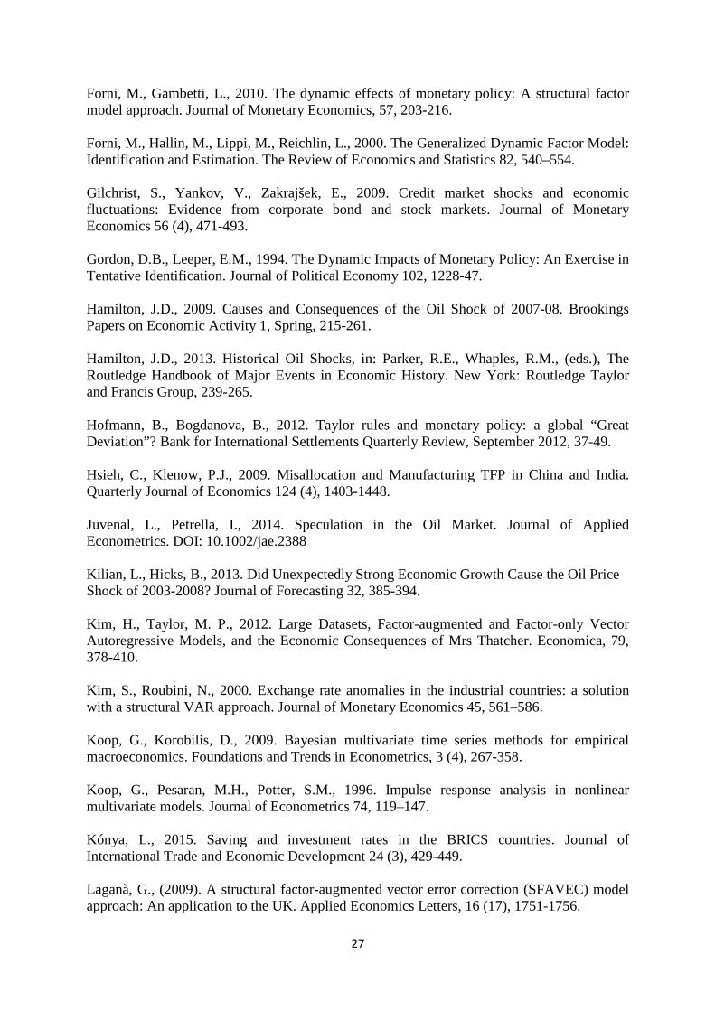
Forni, M., Gambetti, L., 2010. The dynamic effects of monetary policy: A structural factor model approach. Journal of Monetary Economics, 57, 203-216. Forni, M., Hallin, M., Lippi, M., Reichlin, L., 2000. The Generalized Dynamic Factor Model: Identification and Estimation. The Review of Economics and Statistics 82, 540–554. Gilchrist, S., Yankov, V., Zakrajšek, E., 2009. Credit market shocks and economic fluctuations: Evidence from corporate bond and stock markets. Journal of Monetary Economics 56 (4), 471-493. Gordon, D.B., Leeper, E.M., 1994. The Dynamic Impacts of Monetary Policy: An Exercise in Tentative Identification. Journal of Political Economy 102, 1228-47. Hamilton, J.D., 2009. Causes and Consequences of the Oil Shock of 2007-08. Brookings Papers on Economic Activity 1, Spring, 215-261. Hamilton, J.D., 2013. Historical Oil Shocks, in: Parker, R.E., Whaples, R.M., (eds.), The Routledge Handbook of Major Events in Economic History. New York: Routledge Taylor and Francis Group, 239-265. Hofmann, B., Bogdanova, B., 2012. Taylor rules and monetary policy: a global “Great Deviation”? Bank for International Settlements Quarterly Review, September 2012, 37-49. Hsieh, C., Klenow, P.J., 2009. Misallocation and Manufacturing TFP in China and India. Quarterly Journal of Economics 124 (4), 1403-1448. Juvenal, L., Petrella, I., 2014. Speculation in the Oil Market. Journal of Applied Econometrics. DOI: 10.1002/jae.2388 Kilian, L., Hicks, B., 2013. Did Unexpectedly Strong Economic Growth Cause the Oil Price Shock of 2003-2008? Journal of Forecasting 32, 385-394. Kim, H., Taylor, M. P., 2012. Large Datasets, Factor-augmented and Factor-only Vector Autoregressive Models, and the Economic Consequences of Mrs Thatcher. Economica, 79, 378-410. Kim, S., Roubini, N., 2000. Exchange rate anomalies in the industrial countries: a solution with a structural VAR approach. Journal of Monetary Economics 45, 561–586. Koop, G., Korobilis, D., 2009. Bayesian multivariate time series methods for empirical macroeconomics. Foundations and Trends in Econometrics, 3 (4), 267-358. Koop, G., Pesaran, M.H., Potter, S.M., 1996. Impulse response analysis in nonlinear multivariate models. Journal of Econometrics 74, 119–147. Kónya, L., 2015. Saving and investment rates in the BRICS countries. Journal of International Trade and Economic Development 24 (3), 429-449. Laganà, G., (2009). A structural factor-augmented vector error correction (SFAVEC) model approach: An application to the UK. Applied Economics Letters, 16 (17), 1751-1756.
27
Le Bihan, H., Matheron, J., 2012. Price Stickiness and Sectoral Inflation Persistence: Additional Evidence. Journal of Money, Credit and Banking 15, 1427-1442. Lombardi, M. J., Osbat, C., Schnatz, B., 2012. Global commodity cycles and linkages: a FAVAR approach. Empirical Economics 43, 651-670. MacKinnon, J.G., Haug, A.A., Michelis, l., 1999. Numerical Distribution Functions of Likelihood Ratio Tests for Cointegration. Journal of Applied Econometrics 14, 563-577.
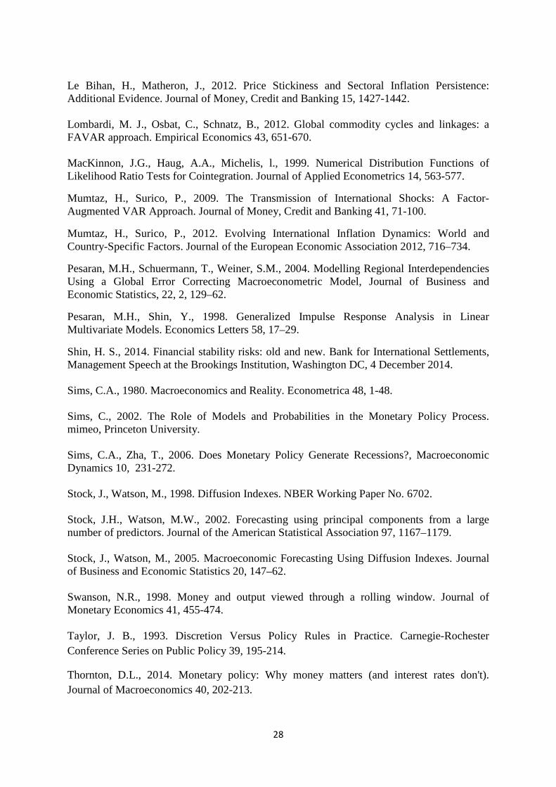
Mumtaz, H., Surico, P., 2009. The Transmission of International Shocks: A Factor-Augmented VAR Approach. Journal of Money, Credit and Banking 41, 71-100.
Mumtaz, H., Surico, P., 2012. Evolving International Inflation Dynamics: World and Country-Specific Factors. Journal of the European Economic Association 2012, 716–734.
Pesaran, M.H., Schuermann, T., Weiner, S.M., 2004. Modelling Regional Interdependencies Using a Global Error Correcting Macroeconometric Model, Journal of Business and Economic Statistics, 22, 2, 129–62.
Pesaran, M.H., Shin, Y., 1998. Generalized Impulse Response Analysis in Linear Multivariate Models. Economics Letters 58, 17–29.
Shin, H. S., 2014. Financial stability risks: old and new. Bank for International Settlements, Management Speech at the Brookings Institution, Washington DC, 4 December 2014. Sims, C.A., 1980. Macroeconomics and Reality. Econometrica 48, 1-48. Sims, C., 2002. The Role of Models and Probabilities in the Monetary Policy Process. mimeo, Princeton University. Sims, C.A., Zha, T., 2006. Does Monetary Policy Generate Recessions?, Macroeconomic Dynamics 10, 231-272. Stock, J., Watson, M., 1998. Diffusion Indexes. NBER Working Paper No. 6702. Stock, J.H., Watson, M.W., 2002. Forecasting using principal components from a large number of predictors. Journal of the American Statistical Association 97, 1167–1179. Stock, J., Watson, M., 2005. Macroeconomic Forecasting Using Diffusion Indexes. Journal of Business and Economic Statistics 20, 147–62. Swanson, N.R., 1998. Money and output viewed through a rolling window. Journal of Monetary Economics 41, 455-474. Taylor, J. B., 1993. Discretion Versus Policy Rules in Practice. Carnegie-Rochester Conference Series on Public Policy 39, 195-214.
Thornton, D.L., 2014. Monetary policy: Why money matters (and interest rates don't). Journal of Macroeconomics 40, 202-213.
28

29

Table 1. Correlation between the logs of country-specific and global variables
Country M2 in US dollars Interest rate Real output CPI Euro area 0.95 0.81 0.89 0.99 US 0.99 0.84 0.90 0.99 China 0.99 0.72 0.71 0.97 Japan 0.92 0.75 0.62 -0.79 India 0.97 0.10 0.70 0.98
Table 2. Test for unit roots 1999:1-2013:12: Data in level
Null hypothesis for ADF test: the variable has a unit root Alternative hypothesis for ADF test: the variable has not a unit root Null hypothesis for KPSS test: variable is stationary Alternative hypothesis for KPSS test: variable is not stationary Level ADF KPSS First difference ADF KPSS log (GM2t) 0.92 1.61*** ∆log (G3M2t) -12.90*** 0.24 log (GCPIt) -1.92 1.52*** ∆log (GCPIt) 1.00*** 0.73 log (GIPt) -2.94* 0.77*** ∆log (GIPt) -4.56*** 0.09 log (GOPt) -2.51 1.51*** ∆log (GOPt) -10.01*** 0.11 log (USTWIt) -0.99 1.41*** ∆log (USTWIt) -9.22*** 0.09
Notes: The first difference of the series is indicated by ∆.The lag selection criteria for the ADF is based on Schwarz information Criteria (SIC) and for the KPSS is the Newey-West Bandwidth. ***, **,* Indicates rejection of the null hypothesis at 1, 5 and 10% level of significance (respectively).
Table 3. LR test Null hypothesis for LR test: no structural change Alternative hypothesis for LR test: structural change
Degree of freedom
𝜒𝜒2 critical value with at 95% 𝜒𝜒2 value
Dummy variable: 2008:M9 to data end 6 12.59 5.95 Dummy variable: 2008:M9 to 2008:M12 6 12.59 39.66*** Dummy variable: 2009:M1 to data end 6 12.59 2.14
Notes: The LR test is 𝐿𝐿𝐺𝐺 = (𝐸𝐸 − 𝑚𝑚)(𝑙𝑙𝑙𝑙|Σ𝐵𝐵| − 𝑙𝑙𝑙𝑙|𝛴𝛴𝐷𝐷𝐵𝐵|)~𝜒𝜒2(𝑞𝑞), where: T is the number of observations, m is the is the number of parameters in each equation of the unrestricted system plus contains, Σ is the determinant of the residual covariance matrix, and q is the number of dummy variables times number of equations.
30
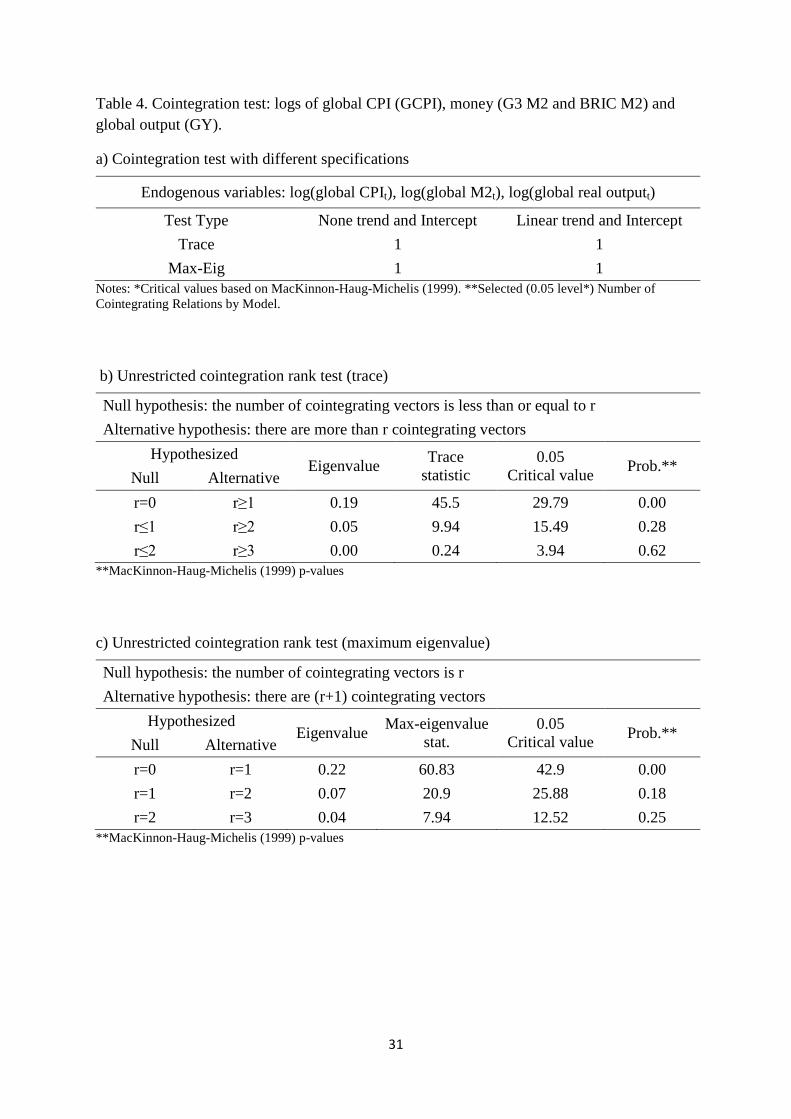
Table 4. Cointegration test: logs of global CPI (GCPI), money (G3 M2 and BRIC M2) and global output (GY).
a) Cointegration test with different specifications
Endogenous variables: log(global CPIt), log(global M2t), log(global real outputt)
Test Type None trend and Intercept Linear trend and Intercept Trace 1 1
Max-Eig 1 1 Notes: *Critical values based on MacKinnon-Haug-Michelis (1999). **Selected (0.05 level*) Number of Cointegrating Relations by Model. b) Unrestricted cointegration rank test (trace)
Null hypothesis: the number of cointegrating vectors is less than or equal to r Alternative hypothesis: there are more than r cointegrating vectors
Hypothesized Eigenvalue Trace
statistic 0.05
Critical value Prob.** Null Alternative r=0 r≥1 0.19 45.5 29.79 0.00 r≤1 r≥2 0.05 9.94 15.49 0.28 r≤2 r≥3 0.00 0.24 3.94 0.62
**MacKinnon-Haug-Michelis (1999) p-values c) Unrestricted cointegration rank test (maximum eigenvalue)
Null hypothesis: the number of cointegrating vectors is r Alternative hypothesis: there are (r+1) cointegrating vectors
Hypothesized Eigenvalue Max-eigenvalue
stat. 0.05
Critical value Prob.** Null Alternative r=0 r=1 0.22 60.83 42.9 0.00 r=1 r=2 0.07 20.9 25.88 0.18 r=2 r=3 0.04 7.94 12.52 0.25
**MacKinnon-Haug-Michelis (1999) p-values
31
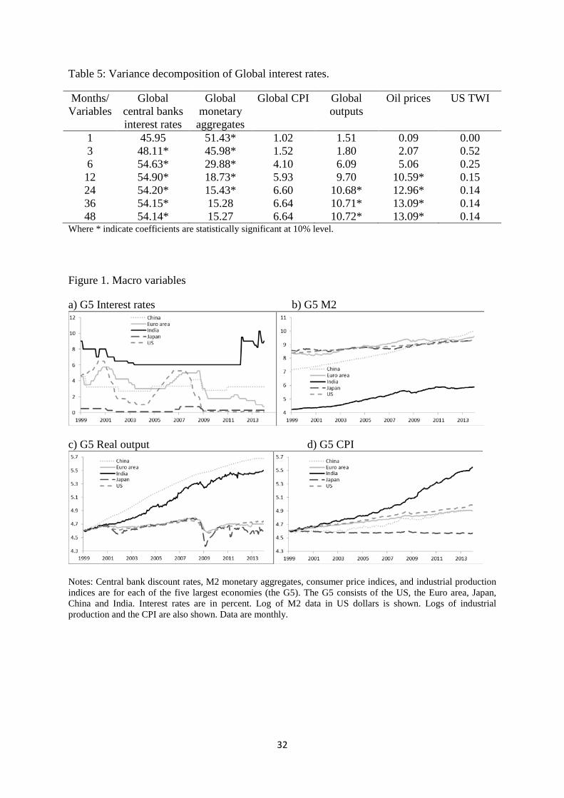
Table 5: Variance decomposition of Global interest rates.
Where * indicate coefficients are statistically significant at 10% level. Figure 1. Macro variables
a) G5 Interest rates b) G5 M2
c) G5 Real output d) G5 CPI
Notes: Central bank discount rates, M2 monetary aggregates, consumer price indices, and industrial production indices are for each of the five largest economies (the G5). The G5 consists of the US, the Euro area, Japan, China and India. Interest rates are in percent. Log of M2 data in US dollars is shown. Logs of industrial production and the CPI are also shown. Data are monthly.
Months/ Variables
Global central banks interest rates
Global monetary
aggregates
Global CPI Global outputs
Oil prices US TWI
1 45.95 51.43* 1.02 1.51 0.09 0.00 3 48.11* 45.98* 1.52 1.80 2.07 0.52 6 54.63* 29.88* 4.10 6.09 5.06 0.25 12 54.90* 18.73* 5.93 9.70 10.59* 0.15 24 54.20* 15.43* 6.60 10.68* 12.96* 0.14 36 54.15* 15.28 6.64 10.71* 13.09* 0.14 48 54.14* 15.27 6.64 10.72* 13.09* 0.14
32
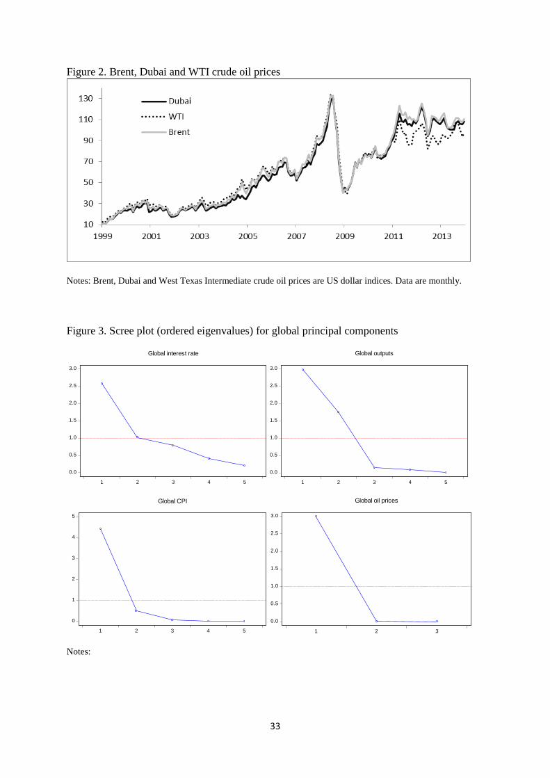
Figure 2. Brent, Dubai and WTI crude oil prices
Notes: Brent, Dubai and West Texas Intermediate crude oil prices are US dollar indices. Data are monthly. Figure 3. Scree plot (ordered eigenvalues) for global principal components
Notes:
0.0
0.5
1.0
1.5
2.0
2.5
3.0
1 2 3 4 5
Global interest rate
0.0
0.5
1.0
1.5
2.0
2.5
3.0
1 2 3 4 5
Global outputs
0
1
2
3
4
5
1 2 3 4 5
Global CPI
0.0
0.5
1.0
1.5
2.0
2.5
3.0
1 2 3
Global oil prices
33
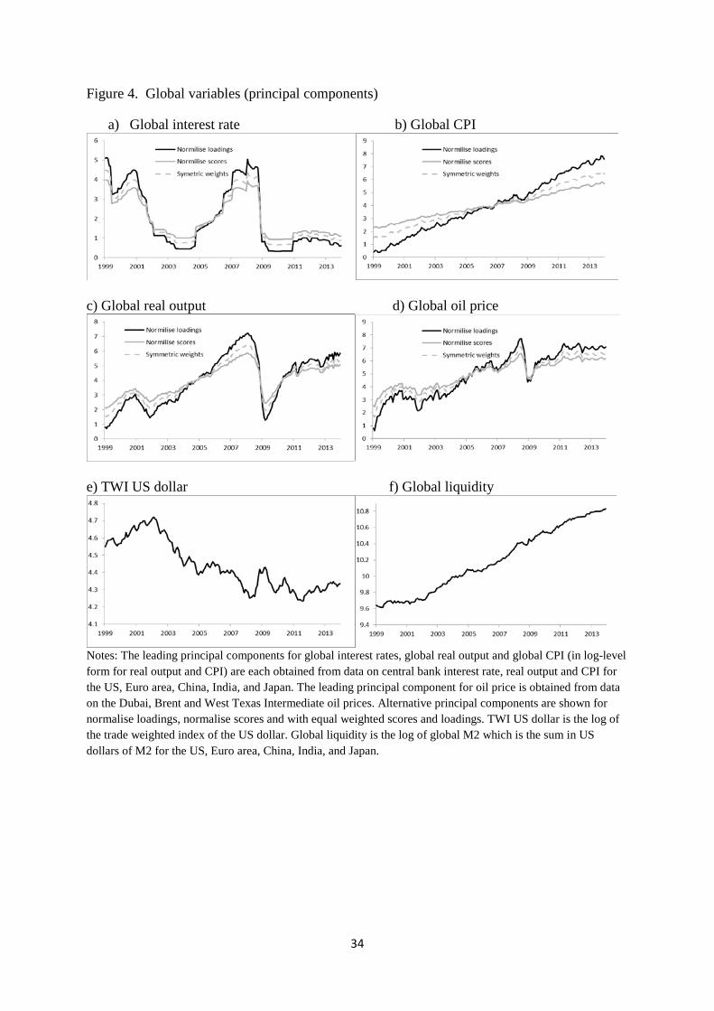
Figure 4. Global variables (principal components)
a) Global interest rate b) Global CPI
c) Global real output d) Global oil price
e) TWI US dollar f) Global liquidity
Notes: The leading principal components for global interest rates, global real output and global CPI (in log-level form for real output and CPI) are each obtained from data on central bank interest rate, real output and CPI for the US, Euro area, China, India, and Japan. The leading principal component for oil price is obtained from data on the Dubai, Brent and West Texas Intermediate oil prices. Alternative principal components are shown for normalise loadings, normalise scores and with equal weighted scores and loadings. TWI US dollar is the log of the trade weighted index of the US dollar. Global liquidity is the log of global M2 which is the sum in US dollars of M2 for the US, Euro area, China, India, and Japan.
34
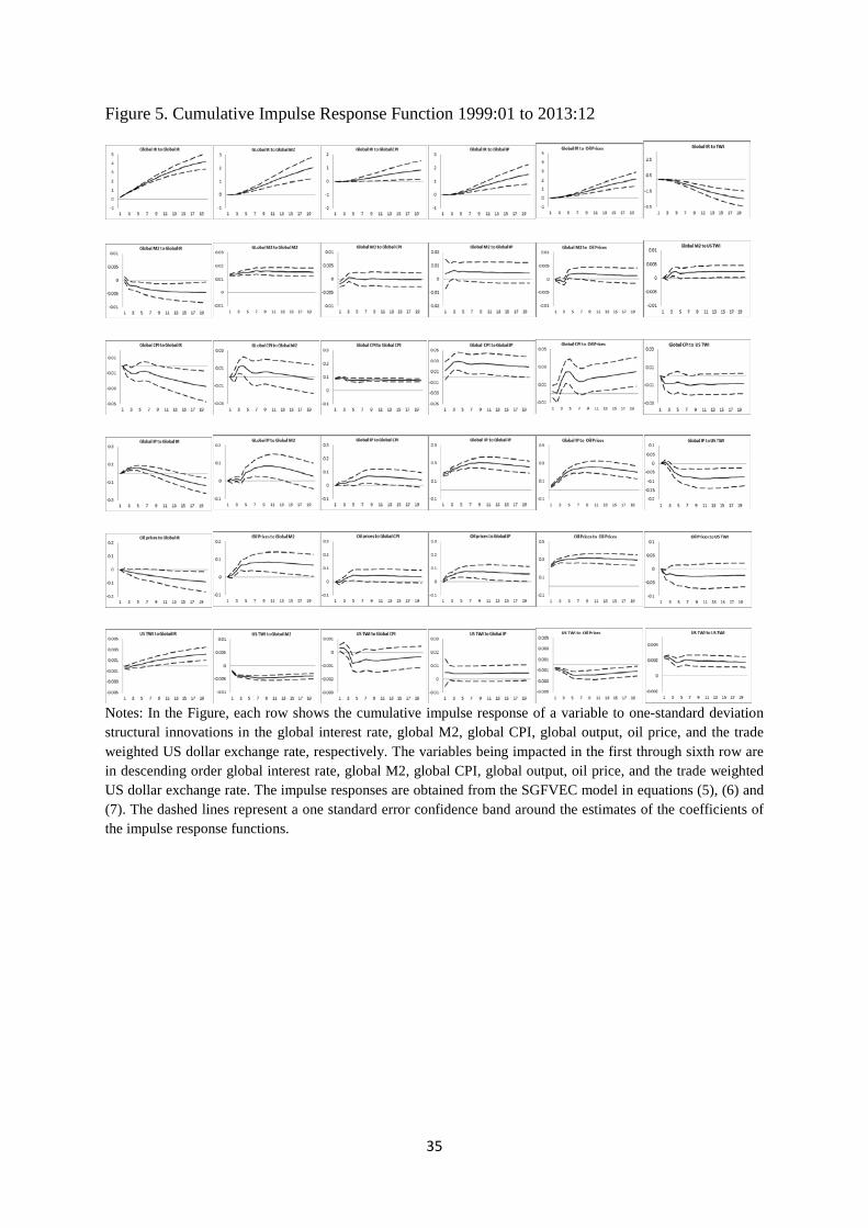
Figure 5. Cumulative Impulse Response Function 1999:01 to 2013:12
Notes: In the Figure, each row shows the cumulative impulse response of a variable to one-standard deviation structural innovations in the global interest rate, global M2, global CPI, global output, oil price, and the trade weighted US dollar exchange rate, respectively. The variables being impacted in the first through sixth row are in descending order global interest rate, global M2, global CPI, global output, oil price, and the trade weighted US dollar exchange rate. The impulse responses are obtained from the SGFVEC model in equations (5), (6) and (7). The dashed lines represent a one standard error confidence band around the estimates of the coefficients of the impulse response functions.
35
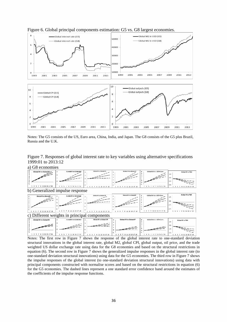
Figure 6. Global principal components estimation: G5 vs. G8 largest economies.
Notes: The G5 consists of the US, Euro area, China, India, and Japan. The G8 consists of the G5 plus Brazil, Russia and the U.K. Figure 7. Responses of global interest rate to key variables using alternative specifications 1999:01 to 2013:12 a) G8 economies
b) Generalized impulse response
c) Different weights in principal components
Notes: The first row in Figure 7 shows the response of the global interest rate to one-standard deviation structural innovations in the global interest rate, global M2, global CPI, global output, oil price, and the trade weighted US dollar exchange rate using data for the G8 economies and based on the structural restrictions in equation (6). The second row in Figure 7 shows the generalized impulse responses in the global interest rate (to one-standard deviation structural innovations) using data for the G5 economies. The third row in Figure 7 shows the impulse responses of the global interest (to one-standard deviation structural innovations) using data with principal components constructed with normalise scores and based on the structural restrictions in equation (6) for the G5 economies. The dashed lines represent a one standard error confidence band around the estimates of the coefficients of the impulse response functions.
36