BOFIT Discussion Papers 16 • 2019

Yiping Huang, Xiang Li and Chu Wang

What does peer-to-peer lending evidence say about the risk-taking channel of monetary policy?

BOFIT Discussion Papers Editor-in-Chief Zuzana Fungáčová BOFIT Discussion Papers 16/2019 29.8.2019 Yiping Huang, Xiang Li and Chu Wang: What does peer-to-peer lending evidence say about the risk-taking channel of monetary policy? ISBN 978-952-323-288-4, online ISSN 1456-5889, online The views expressed in this paper are those of the authors and do not necessarily represent the views of the Bank of Finland. Suomen Pankki Helsinki 2019

What Does Peer-to-Peer Lending Evidence Say About

the Risk-taking Channel of Monetary Policy? ∗

Yiping Huang † Xiang Li ‡ Chu Wang §

August 2019

Abstract

This paper uses loan application-level data from a peer-to-peer lending platform to

study the risk-taking channel of monetary policy. By employing a direct ex-ante

measure of risk-taking and estimating the simultaneous equations of loan approval

and loan amount, we are the first to provide quantitative evidence of the impact of

monetary policy on the risk-taking of nonbank financial institution. We find that

the search-for-yield is the main workhorse of the risk-taking effect, while we do

not observe consistent findings of risk-shifting from the liquidity change. Monetary

policy easing is associated with a higher probability of granting loans to risky

borrowers and a greater riskiness of credit allocation, but these changes do not

necessarily relate to a larger loan amount on average.

Keywords: Monetary Policy, Risk-taking, Nonbank Financial Institution, Peer-

to-Peer Lending, Search-for-yield, Risk-shifting

JEL Codes: E52, G23

∗We would like to thank, for comments, discussion and suggestions from Jia Chen (discussant), Se-bastian Di Tella, Zuzana Fungacova (discussant), Michael Funke, Jon Frost, Iftekhar Hasan, KeweiHou, Yi Huang, Matt Klepacz, Michael Koetter, Iikka Korhonen, Kai Li, Xiaoyang Li (discussant), YeLi, Laura Xiaolei Liu, Konstantin Milbradt, Gernot Muller, Mark Spiegel, Marc Stoeckli (discussant),Javier Suarez, and other scholars in the IWH Macroeconomics Seminar, 2018 Guanghua InternationalSymposium of Finance, Birmingham Business School and the Journal of Corporate Conference on De-velopments in Alternative Finance, 2019 CESifo Area Conference on Macro, Money and InternationalFinance, CEBRA 2019 Annual Meeting, and 2019 BOFIT Conference on China’s Progress to “Moder-ately Prosperous Society”. Any errors remain ours alone.†National School of Development, Peking University. No.5 Yiheyuan Road, Haidian District, Beijing,

100871, China. Email: yhuang@nsd.pku.edu.cn ORCID: orcid.org/0000-0002-8378-4087‡Corresponding author. Halle Institute for Economic Research (IWH). Kleine Maeker-

strasse 8, Halle(Saale), 06108, Germany. Email: Xiang.Li@iwh-halle.de ORCID: orcid.org/

0000-0002-4738-0034§National School of Development, Peking University. No.5 Yiheyuan Road, Haidian District, Beijing,

100871, China. Email: wangchu@pku.edu.cn ORCID: orcid.org/0000-0003-2004-1726

1 Introduction

The risk-taking channel of monetary policy has attracted more attention since the global

financial crisis. A low interest rate and lax monetary environment have been accused of

giving rise to the higher risk preference of financial institutions, which was at the root of

the financial tsunami (Adrian and Shin 2008, 2009, Angeloni and Faia 2013, Bernanke and

Reinhart 2004, Mishkin 2011, Schularick and Taylor 2012, Taylor 2009). This channel,

if it holds true, implies that monetary policy goes far beyond the traditional impact on

price stability and economic growth; it also has implications for systemic risk and financial

stability (Borio and White 2004, Issing 2003, Smets et al. 2014, Stein 2012). Expansionary

monetary policy can result in the increase of credit quantity (Gambacorta and Marques-

Ibanez 2011, Kashyap and Stein 2000) as well as the decrease in credit quality (Borio and

Zhu 2012, Jimenez et al. 2014). Therefore, the relationship between monetary policy and

macroprudential management becomes more convoluted and challenges the policymakers.

The answers to the question of whether and how monetary policy affects risk-taking are

pivotal to the policy discussion and of great academic interest.

This paper studies the risk-taking channel of monetary policy based on the evidence

from peer-to-peer (P2P, henceforth) lending. Specifically, we intend to answer the follow-

ing three questions. First, whether the P2P platform’s risk tolerance increases through

higher probabilities and larger loan amounts to riskier borrowers when monetary policy

eases. Second, what is the mechanism behind the risk-taking channel. In particular, this

study investigates whether the search-for-yield and funding liquidity play a role in the

risk-taking channel. Third, the tightening of regulation policy for the P2P industry in

China provides a good experiment to study whether the financial regulation policies can

curb the increased risk-taking during the expansionary monetary policy period.

Using loan application-level data, we establish new evidence for the risk-taking channel

of monetary policy. The main findings are threefold. To begin, a financial institution

tends to take more risks when monetary policy eases by lending to riskier borrowers.

Meanwhile, the impact of the increased funding liquidity in the liability side on risk-

taking is ambiguous. In addition, stricter regulation is effective in limiting the increased

risk-taking from the eased monetary policy.

This study contributes to the literature from the following perspectives. The first

is the measurement of ex-ante risk-taking. The key point of the risk-taking channel in

comparison with the credit channel or balance sheet channel is in the risk perception and

ex-ante risk-taking of financial institutions. Previous studies mostly rely on the survey

data of bank lending standards (Dell’Ariccia et al. 2017, Paligorova and Santos 2012,

Maddaloni and Peydro 2011) or loan-level data of previous firms’ default information

1

(Ioannidou et al. 2014, Jimenez et al. 2014). We have the credit scores of each loan

applicant, which are developed by the P2P platform based on big data, and the loan

application results, which allow us to capture the institution’s loan approval decision and

use the credit scores of approved and rejected applicants to directly measure risk-taking

and study the relationship between risk and return.

Second, we are the first to provide evidence of risk-taking from a non-bank financial

instituion. According to Adrian and Shin (2009) and Adrian and Shin (2010a), as the

economy becomes more increasingly market-based, the shadow banking system becomes

more important in conveying information about the credit conditions running the econ-

omy. Moreover, the reason that Rajan (2006) focus on the incentives of managers with

investors and the nature of risks undertaken by the system is that investment managers

have displaced banks and reintermediate themselves between individuals and markets,

while banks are moving to more illiquid transactions, where explicit contracts are hard

to specify or where the consequences need to be hedged by trading in the market. The

same argument applies to the emphasis on the nonbank financial intermediary in this

study. In addition, for these nondepository institutions, their liabilities are funds from

other investors and the search-for-yield incentive can be stronger with the absence of

deposit insurance. The risk management in nonbank financial institutions, such as the

P2P platforms, is essential to understanding the risk in the financial system. Moreover,

the nonbank financial institution in this study is a FinTech internet lending company.

FinTech allows the loan officers to obtain accurate and timely information much more

efficiently and to reduce monitoring efforts (Rajan 2006), thus becoming more focused

on searching for yields and responding to policy changes. It also generates advantages by

providing a better measurement of ex-ante risk-taking. Big data and financial technology

allow lenders to collect the borrowers’ information at a greatly reduced cost and largely

improved speed; thus, their perception of risk is more descriptive, and their reaction to

monetary policy change is more prompt. Because of the limits in the literature, a more

accurate measurement of risk-taking and evidence from a FinTech nonbank financial in-

stitution can carry the study a step forward.

In addition, we provide evidence from a large emerging economy. Most existing studies

use US data, for instance Dell’Ariccia et al. (2017), Altunbasa et al. (2014), Buch et al.

(2014b) and Delis et al. (2017). Others use datasets from European banks, including

Jimenez et al. (2014), using Spain data; Gersl et al. (2015), using data from the Czech

Republic; and Gaggl et al. (2010), using Austrian data. The only exception from a

developing country is Ioannidou et al. (2014), who use Bolivian data. Our evidence from

China also fills in the gap of the literature.

There are two main mechanisms in the literature which are used to explain the risk-

2

taking channel of monetary policy. The first is the search-for-yield. Financial institutions

usually enter into long-term contracts with a significant percentage of their borrowers and

investors involving a commitment to produce a certain nominal rate of return, and they

need to match this return to their liabilities based on their assets (Altunbasa et al. 2014,

De Nicolo et al. 2010, Rajan 2006). When monetary policy eases, the nominal return

of the previous investment portfolio also goes down. To reach the committed nominal

return, the managers of the financial intermediary would turn to riskier investments. As

documented in Gambacorta (2009) and BIS (2004), in 2003-2004, many investors shifted

from low-risk government bonds into higher-yielding but riskier corporate and emerging

market bonds. They were seeking to meet the nominal returns they had been able to

achieve when interest rates were higher. Moreover, for behavioral reasons, investors

tend to use the short-term return as a way to judge the managers’ competence and this

judgment is related to the managers’ compensation and the assets they can obtain(Rajan

2006). Thus, the managers are encouraged to increase the risk exposure, especially in the

periods of low interest rates because the incentive to search for yield goes up. Altunbasa

et al. (2014) use the panel dataset of listed banks in Europe and the US and find that

low levels of interest rates over an extended period of time contributed to an increase in

the banks’ risk. Buch et al. (2014a) also confirm a search-for-yield mechanism by using

the US bank survey dataset and documenting that small domestic banks increase their

exposure to risk following an expansionary monetary policy shock.

The second mechanism is risk-shifting and the pass-through. Dell’Ariccia et al. (2017)

provide a simple model of interest rates, leverage, and bank risk-taking1. They capture the

banks’ risk-taking through the incentives to monitor by modeling both the risk-shifting

and pass-through effects. This is how the risk-shifting effect works: when the reference

rate reduces, bank funding is cheaper; the profits in the event of success increases, and

the financial distress decreases, which leads to higher monitoring incentives and less risk-

taking. However, there is also a pass-through effect, as the reduced monetary policy

rate leads to a lower lending rate; then, the profits and incentive to monitor decrease,

which indicates more risk-taking. The implications are that bank risk-taking is negatively

associated with the policy interest rate, but this effect is less pronounced when the bank

is poorly capitalized and has a higher leverage. According to this model, the risk-taking

relates to both the reference rate and the banks’ capital structure, and it depends on the

relative strength of risk-shifting and pass-through. 2 However, this might be the place

1The model is in the Appendix A of Dell’Ariccia et al. (2017).2Similarly, De Nicolo et al. (2010) argues that if the financial institution has a high level of liability

compared to its own capital, it can enjoy larger spread and profits when monetary policy eases, thus ithas less incentive to take risks. This is because lower policy rate transmits more efficiently to the liabilityside than the asset side of financial intermediaries, thus spreads increase and lead to larger profits. Whenthe financial intermediary has more skin in the game, especially when liability increases in relative to

3

where the difference between banks and nonbanks matter. As we will see in section 3.2, for

the Chinese P2P lending market, its financial return on the liability side is rather stable

and maintained at a high level to compete with bank deposits, of which the adjustment

in face of monetary policy is limited. If the cost of funding is relatively inelastic to the

monetary policy, then the risk offsetting effect of reduced financial distress could be small.

Furthermore, the additional availability of liquidity after the monetary policy loosens

(Buch et al. 2014a) may also induce risk-taking. On one hand, the value-at-risk con-

straints are weakened with more liquidity. On the other hand, adverse selection problems

in the credit market are mitigated; thus, the financial intermediary’s screening incentives

are reduced, and the financial institution becomes more risk-taking. 3

There is also macro evidence in support of the risk-taking channel4, though most

studies as well as this paper use bank-level or loan-level micro data. For instance, Bekaert

et al. (2013) find that a lax monetary policy decreases risk aversion, Angeloni and Faia

(2009) document that a monetary restriction reduces leverage using a DSGE model of

prudential regulation and monetary policy with fragile banks, and Kodres et al. (2008)

find that emerging market spread falls significantly when industrial country interest rates

fall unexpectedly and when the interest rate volatility is low.

There are five major challenges for empirically identifying the risk-taking channel of

monetary policy, and the loan application-level dataset in this paper works well in cop-

ing with these challenges. First, it is difficult to accurately measure ex-ante risk-taking.

Most papers use the bank performance indicators such as bank leverage, VaR, Z-score,

risk-weighted asset ratio, loan default rate, or market volatility measures and others,

equity, it is less likely to take more risks, vice versa.3There are other factors that are claimed to be the workforce of the risk-taking channel, such as the

impact on real valuation of the financial intermediary’s liabilities and assets mentioned in Delis et al.(2017) and Gaggl et al. (2010). However, we believe this is the crucial element of the broad credit channeland not the heart of the risk-taking channel.

4It is important to distinguish the risk-taking channel from other monetary policy transmission chan-nels. Many existing studies use the impact of monetary policy on the health of financial intermediariesin terms of leverage and asset quality to claim the risk-taking channel. However, it is different from theimpact on the perception of risk and the willingness to bear risk, and it is the result of bank lending andbalance sheet channel instead of the risk-taking channel (Lopez et al. 2012). For instance, Adrian et al.(2018) show that when monetary policy tightens, the term spread reduce, net interest margin lower, andcredit supply is reduced, vice versa. Thus, they claim that the relationship between expansionary mone-tary policy and more credit supply is evidence of risk-taking channel. Valencia (2014) also document thatthe lower funding cost from lower risk-free rate incentives the banks to increase lending and thus leverage.As we can see, Adrian et al. (2018) and Valencia (2014) focus on the quantity effect of monetary policy,however, the risk-taking channel of monetary policy should focus on the risk appetite of the financialintermediary and the credit quality instead of credit quantity. Although Adrian and Shin (2010b) arguethat balance sheet quantities emerge as a key indicator of risk appetite and hence for the risk-takingchannel of monetary policy, a more direct measure of risk appetite would contribute to disentangle therisk-taking channel from the bank lending channel. In this sense, modeling the monitoring incentive inDell’Ariccia et al. (2017) is closer to the essence of risk-taking channel than modeling the credit supplyin Adrian et al. (2018).

4

to indicate risk-taking5. In fact, these indicators are the results of the financial insti-

tutions’ risk management decisions instead of the risk tolerance itself. These ex-post

measurements are simultaneously determined by lenders’ risk perception and the bor-

rowers’ ability to pay; thus the pure effect of the risk-taking channel cannot be isolated,

as both can be affected by monetary policy. In our dataset, we observe each loan ap-

plication, including whether or not the loan is granted, and a rich set of the applicants’

characteristics, including credit score, basic demographic information, mobile contacts,

credit card history and online shopping behavior. We use the borrowers’ credit scores at

the time of loan application to measure each loan’s ex-ante risk. This score is determined

before the loan takes place and it is calculated based on big data to reflect the borrower’s

credit quality. In addition, we also have each borrower’s overdue history in other loans,

which can also be employed as an ex-ante indicator of riskiness.

Second, monetary policy may be endogenous to financial stability. If monetary policy

is eased because of a stable financial market or tightened because of a volatile financial

market, then the finding of more risk-taking with an easing monetary policy is likely

to be underestimated. Alternatively, if the agents in the financial market see an easing

monetary policy as a signal of a stable financial condition, then they may engage in

riskier behaviors and the findings tend to be overestimated. Two approaches are adopted

in this paper to deal with the possible endogeneity of monetary policy. First, we analyze

the contents of the Monetary Policy Executive Report to gauge the attention given to

financial stability in monetary policy, following Dell’Ariccia et al. (2017). We find that

the frequency of mentioning financial stability is relatively low (See Appendix). Second,

in the spirit of the argument in Jimenez et al. (2014), the monetary policy is country-wide

and should be universal to different provinces. Thus, we control the province fixed effect

in the estimation given that the monetary policy should be exogenous at the province-

level.

Third, it is difficult to isolate the impact on credit supply and credit demand. If a

reduced monetary policy rate is associated with a higher loan demand from riskier bor-

rowers, then the essence of the risk-taking channel of monetary policy, i.e., the increased

risk-preference of the credit supplier, is mixed with riskier profiles on the demand side.

Our data is fitted to alleviate this concern in the following ways. First, we have the overall

loan application entries, which include not only the loans that are granted but also those

which are rejected. Even if the borrower profile changes with the monetary policy, the

granting process is fully controlled by the credit supplier and it is their key step of risk

management. Therefore, an investigation of the probability for similar applicants to be

granted the loan, in terms of ex-ante credit scores, would be able to isolate the impact of

5A detailed discussion of the measurement can be found in section 2.

5

demand. Second, we use the total amount of all loan applications in each day (including

the rejected ones), to construct a proxy for aggregate demand. In addition, the number

of borrowers in the overall P2P market is another proxy for credit demand, though at a

lower frequency (monthly). We control these demand proxies in the regression, and the

risk-taking findings still hold.

Fourth, the impact of monetary policy on loan amount can be biased without a

consideration of loan granting. In addition to testing whether the loans are allocated to

riskier borrowers when the monetary policy eases, we are also interested in how the loan

amount changes. If the loan amounts decrease, even the borrowers become riskier, and

the increase in riskiness for the financial institution and financial system can be limited.

Moreover, using the observations of whose loan applications are granted leads to biased

results, as shown in Jimenez et al. (2014). Benefiting from the data structure, we are able

to conduct a similar two-step analysis to first estimate the probability of loan granting

and then the granted loan size.

Fifth, it is necessary to distinguish the impact from monetary policy on existing loans

and new loans. Buch et al. (2014b) distinguish the forward-looking and backward-looking

bank risk because lower interest rates may reduce risk as the firms’ interest burden

is lowered, and the value of the collateral increases; thus, the repayment probability

increases. This increase can lead to a decreased risk of existing loans but not new loans.

Moreover, this also strengthens the necessity to use ex-ante risk-taking measurement

instead of ex-post measurement. Our dataset focuses on the new loan applications; thus,

it is not affected by the existing loans and purely reflects the change in risk-perception

of the financial institution.

Finally, we admit several drawbacks of this study. First, this study leaves blank the

impact of monetary policy on pricing, collateral requirement and actual default proba-

bilities over the life of the loan as we only have the information on the application and

approval stage but not over the life of the loan. However, based on the research that

has investigated these perspectives, such as Ioannidou et al. (2014), there is assurance

that a financial institution does not compensate for the extra risk taken by adjusting

loan conditions, such as loan price and collateral values. Buch et al. (2014a) also find

that the increase of the risk composition of loan portfolios is not compensated by higher

risk premia6. In addition, there are studies using the loan pricing as indicators of risk-

taking which conclude that the spreads to riskier borrowers relative to the spreads to

safer borrowers become lower during the periods of low short-term rates.

Second, though it is innovative enough to provide evidence from a nonbank financial

6Loan spread is measured as the difference between risky loan rate and the riskless loan rate proxiedby 1-year treasury bond rate.

6

institution such as a P2P lending platform, we only have the dataset of one specific

platform and cannot control the platform fixed effect. Though we provide statistics to

show it is a typical P2P platform in China, we can only observe the lending relationships

of each borrower who has applied multiple times in the same platform at different times,

but not each borrower who applies to multiple financial institutions at the same time.

Thus, we cannot completely isolate the impact of monetary policy on the demand side

and the supply side as the specification in Jimenez et al. (2014), which uses bank fixed

effects in addition to borrower fixed effects to control the heterogeneity among credit

suppliers.

This study provides meaningful policy implications. First, consistent with Berger and

Udell (2004), a financial intermediary takes more risks during monetary policy expansion,

but the risks are only revealed later because it takes time to expose the loan performance

problem. Thus, the implication is that the regulators should closely watch the unnoticed

buildup of financial risks during the periods of low interest rates. Our analysis period is

August 2017 to April 2018, during which the monetary policy generally eased. Increased

risk-taking during the monetary policy easing is accumulated to break out a wave of

default of P2P platforms in the summer of 20187. Second, monetary policy should take

account of its effect on incentives. The competition to attract funding in the P2P market

results in a pseudocommitment to high financial returns for investors, and this intensifies

the search-for-yield mechanism when monetary policy rate is low. Third, the statistics

from banks may no longer be sufficient for the quality of financial activities and pru-

dential regulations should apply to address perverse behaviors in the nonbank financial

institutions. Monetary policy should be coordinated with prudential regulation policies

to balance the economic growth and financial stability.

The paper is structured as follows. Section 2 describes the loan application-level data

and monetary policy variables used in the paper. Section 3 develops the hypotheses in

empirical analysis based on the theoretical background and raw evidence from the data.

Section 4 shows three empirical designs and presents the results. Section 5 discusses

further concerns related to this study. Section 6 conducts several robustness checks.

Section 7 concludes.

7There are over 200 P2P platforms defaulted in the single month of July in 2018.

7

2 Data and Variables

2.1 P2P Loan Applications and Contracts

The loan application-level data comes from a P2P internet lending platform in China.

First of all, it is necessary to point out the specific practice of peer-to-peer lending in

China. There are different business models of peer-to-peer lending. The first type of

platforms are more like information intermediary, which allow individual borrowers to

publicly list their loan demands and then individual lenders to view the listings and choose

which to lend. The P2P platforms in the US and Europe are more of this type. The

other type of platforms are more like credit intermediary, which package the loan targets

and then individual lenders choose products with certain maturity and investment return

without knowing specific loan listings or specifying the borrower pools they are investing

in. And the platforms are in charge of the success or failure of each loan listing. The first

type of P2P platforms also exist in China, such as Renrendai in its early stage. But the

second type of platforms becomes more and more popular as the first type requires much

efforts from individual lenders and thus limit the scale and profitability of the platform.

Moreover, due to the immature credit scoring system, the credit intermediary type of

P2P platforms are typical in China, including the one we from which we obtain the

data8. Thus, more and more P2P platforms in China play the role of nonbank financial

intermediaries rather than merely information intermediaries, and they are sensitive to

the macro environment and monetary policy adjustments. We provide a figure of the

business model of this P2P platform in the appendix A2.

Equipped with FinTech and big data, the P2P platform closely monitor the borrower

profiles9 and optimize the loan granting using information from their credit history and

digital footprints. We observe loan characteristics including whether or not the loan is

granted, the loan amount, maturity and interest rate. In addition to gender and age, we

observe rich applicant characteristics including the information from mobile carriers such

as the borrowers’ amount of calls in number and time length; their contact with family

and other call habits; the information from the credit card reported by the borrowers

such as their transactions in the past 12 months; number of cards and banks; history

of cash out, interest payment, credit line usuage and overdue count as well as amount;

8Due to disclosure principles, we hide the name of this platform. Later we show its representativenessin the aggregated P2P industry, and the desensitized data for results replication is available with thepublication of the paper.

9It is worth noticing that the platform sets a very low entry barrier for borrowers, as the minimumrequirement is to have a mobile phone and a national identity card, thus there is little pre-screen issueshere. In contrast, it usually requires income certificates or real estate to proofs to start a loan applicationin banks.

8

and implicit income and credit card information from Alipay10. Most importantly, we

observe the credit score for each applicant. Unlike the FICO score which is based on

the hard information from credit card history, the P2P platform employs an algorithm

to assess the riskiness and probability of delinquency of each registered user based on

all the observed characteristics mentioned above. The official credit information system

is heavily criticized in China, and it is common for financial institutions with FinTech

and big data to develop independent credit score algorithms to manage risk11. For the

pricing policy, the interest rate of each loan is determined by the credit score and loan

maturity.12

As described in the introduction, there are several advantages to using this dataset

to investigate the risk-taking channel of monetary policy. First, the credit score provides

an excellent measurement of ex-ante risk-taking because it is a direct judgment by the

platform before the loan contract comes into effect of the borrowers’ trustfulness and

probability of default. Most papers use the bank performance indicators such as leverage,

VaR, Z-score, risk-weighted asset ratio, loan default rate, or market volatility measures,

such as VIX and others, to indicate risk-taking (Adrian and Shin 2010c, Adrian et al.

2018, Bruno and Shin 2015, Cebenoyan and Strahan 2004, Esty 1998, Khan et al. 2017,

Laeven and Levine 2009, Lopez et al. 2011). However, these indicators are the results of

financial institutions’ risk management decisions instead of the risk tolerance itself. These

ex-post measurements are simultaneously determined by the lenders’ risk perception and

the borrowers’ ability to pay; thus, the pure effect of the risk-taking channel cannot be

isolated as both can be affected by monetary policy. Recently, papers have employed

quasi-ex-ante risk indicators. For instance, Jimenez et al. (2014) and Gersl et al. (2015)

evaluate the loan risk based on the borrowers’ credit history of whether they have had

nonperforming loans, which is an improvement but still quite coarse; Buch et al. (2014b)

use the share of noninterest income to total income; Delis et al. (2017) use the loan-

specific coupon spread as a markup over LIBOR; Lopez et al. (2012) use the ratio of the

loan amount to risky borrowers to safe borrowers; and Maddaloni and Peydro (2011) use

the survey data to measure the lending standard. Borrowers’ credit scores would be a

significant improvement to capture the financial institution’s perception of risk.

Second, the dataset allows the estimation of the probit and selection model in section

10A popular third-party mobile and online payment platform in China.11The most known credit score system in China may be the Sesame credit scores from Alipay. The

P2P platform in this paper develops its own credit score system and it is different from the Sesame creditscores. Especially, the loan applicants do not observe their own credit scores in our data, and the creditscores here do not update as frequently as the Sesame credit scores.

12This is similar to the LendingClub, the interest rates in which are determined by FICO score, debt-to-income ratio, credit history, loan amount and loan maturity. In the platform we study, the creditscore has already taken into account the information including debt-to-income ratio and credit history,and have accounted for additional information from the big data.

9

4 based on the observation of both granted and rejected loan applications. One of the

most important steps in risk management is loan granting. The decision of which loan

applications to approve and which to reject largely captures the risk perception of the

financial institution. An investigation into the change of riskiness of the granted loan

borrowers with a different monetary policy environment is a good way to see how the

monetary policy affects risk-taking, and this is the method used in most studies and in

the first baseline results of this paper. However, the probability of obtaining the loan and

the granted loan amount for borrowers with different riskiness as the monetary policy

eases or tightens provides richer information, and it requires data for both rejected and

granted loan applications. The dataset in this paper makes it possible to estimate a

selection model of loan granting and loan amount, similar to the one adopted in Jimenez

et al. (2014).

Third, the dataset focuses on new loans and exclude existing loans and thus can

separate the new risk from the realized risk. A reduced monetary policy rate may affect

the default probability of existing loans because it brings down the financing pressure of

firms. Thus, the realized risk decreases while the new risk increases, making the overall

risk undetermined. By only including the new loan applications, the dataset in this paper

excludes the impact on existing loans and the effect of the lower probability of default of

outstanding loans during low interest rate periods.

The P2P loan data to which we have access is a 10% random sample of the loan

applications on each day from the beginning of August 2017 to the end of March 2018.

We clean the data by dropping 19 applications from individuals who are on the credit

black list from the supreme court, and dropping the days on which the loan granting

ratio is lower than the 1st or higher than the 99th percentile. To make the results

comparable across specifications, the sample contains only borrowers that apply more

than once. We have a total of 73,264 loan applications, of which 13,266 are granted,

and these applications come from 17,344 borrowers, 6,498 of which have been approved

a loan. Table 1 and Table 2 present the summary statistics of the dataset we use in this

paper.

Figure 1 demonstrates the representativeness of the loan dataset from the specific

P2P platform in this paper by plotting the time-series of the granted loan amount in our

sample and that of an aggregated index designed to capture the overall development of

the P2P industry in China. It shows that the two series move together, indicating that

the dataset in this study has a consistent pattern similar to the aggregated P2P industry.

For a better illustration, we use weekly data in the figure by aggregating the granted loan

amount for each week and by taking the weekly average of the original daily P2P industry

development index. The pairwise correlation of the two series is 0.41 and is significant at

10

1%.

Figure 2 shows the histogram of the granted loan amount and maturity in the data.

Over 90% of the granted loans are smaller than 40,000 yuan (approximately 6,150 dollars

using an exchange rate of 6.5 RMB/USD), and more than 80% have the tenor within

one year. Statistics also show that the mean and median of the loan amounts are 17,500

yuan (approximately 2,700 dollars) and 13,000 yuan (approximately 2,000 dollars). It

should be noted that we are unable to identify the usage of the loans, nor can the P2P

platform as it does not restrict the usage except for warnings to the borrowers that the

loan cannot be used for a real estate downpayment. Judging from the average size and

maturity of the loan, a plausible hypothesis would be that most of the loans are applied

for consumption use or a small business operation. Using consumer loans to investigate

the risk-taking channel is supported by Maddaloni and Peydro (2011), who document

that the risk-taking channel also holds for household loans.

Another loan characteristic in which we are interested is the borrowing interest rate

and investing return of the P2P platform. The search-for-yield hypothesis assumes that

the return for investors (burdened by the P2P platform) is more stable relatively, than

the loan interest rates, and adjusts to a lower frequency when the monetary policy rate

changes. Although we cannot access the investor return data for the specific P2P platform

in this paper, we have the daily composite return of the wealth management products of

the overall P2P industry from WDZJ13. Figure 3 shows the time-series of the industry-

level investment return rates and the daily average loan interest rates from the specific

P2P platform. First, the spread between the interest rates for borrowers and investors are

as large as over ten percentage points. Second, the return for P2P investors stay relatively

stable across the sample periods. The average return is 8.60% and the standard error

is 0.3. Third, even when we take the average from one specific P2P platform, the loan

interest rates are very volatile, with the average rate at 19.61% and standard error at 1.68.

These observations indirectly validate the search-for-yield hypothesis in the literature.

2.2 Monetary Policy Environment and P2P Industry

China has a monetary policy framework that is quite different from that of the advanced

economy. According to the official documents, China’s monetary policy is not inflation-

targeting and not Taylor-rule based, although the empirical evidence is ambiguous (Bur-

dekin and Siklos 2008, Zhang 2009, Liu and Zhang 2010, Xiong 2012). Moreover, it is in

transition from quantity-based to price-based and the current state is a hybrid. To save

space, we present a detailed description of the background of China’s monetary policy in

13An information platform for the Chinese P2P market, it provides daily statistics of the industry.

11

the appendix14.

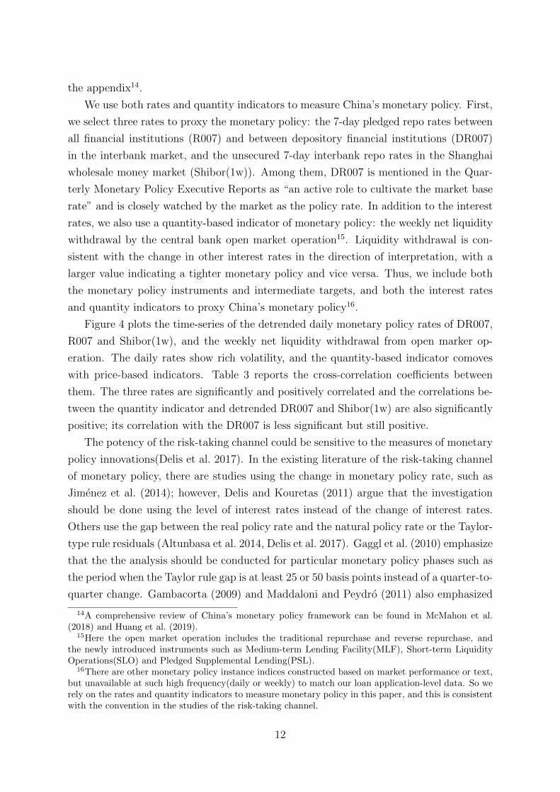
We use both rates and quantity indicators to measure China’s monetary policy. First,

we select three rates to proxy the monetary policy: the 7-day pledged repo rates between

all financial institutions (R007) and between depository financial institutions (DR007)

in the interbank market, and the unsecured 7-day interbank repo rates in the Shanghai

wholesale money market (Shibor(1w)). Among them, DR007 is mentioned in the Quar-

terly Monetary Policy Executive Reports as “an active role to cultivate the market base

rate” and is closely watched by the market as the policy rate. In addition to the interest

rates, we also use a quantity-based indicator of monetary policy: the weekly net liquidity

withdrawal by the central bank open market operation15. Liquidity withdrawal is con-

sistent with the change in other interest rates in the direction of interpretation, with a

larger value indicating a tighter monetary policy and vice versa. Thus, we include both

the monetary policy instruments and intermediate targets, and both the interest rates

and quantity indicators to proxy China’s monetary policy16.

Figure 4 plots the time-series of the detrended daily monetary policy rates of DR007,

R007 and Shibor(1w), and the weekly net liquidity withdrawal from open marker op-

eration. The daily rates show rich volatility, and the quantity-based indicator comoves

with price-based indicators. Table 3 reports the cross-correlation coefficients between

them. The three rates are significantly and positively correlated and the correlations be-

tween the quantity indicator and detrended DR007 and Shibor(1w) are also significantly

positive; its correlation with the DR007 is less significant but still positive.

The potency of the risk-taking channel could be sensitive to the measures of monetary

policy innovations(Delis et al. 2017). In the existing literature of the risk-taking channel

of monetary policy, there are studies using the change in monetary policy rate, such as

Jimenez et al. (2014); however, Delis and Kouretas (2011) argue that the investigation

should be done using the level of interest rates instead of the change of interest rates.

Others use the gap between the real policy rate and the natural policy rate or the Taylor-

type rule residuals (Altunbasa et al. 2014, Delis et al. 2017). Gaggl et al. (2010) emphasize

that the the analysis should be conducted for particular monetary policy phases such as

the period when the Taylor rule gap is at least 25 or 50 basis points instead of a quarter-to-

quarter change. Gambacorta (2009) and Maddaloni and Peydro (2011) also emphasized

14A comprehensive review of China’s monetary policy framework can be found in McMahon et al.(2018) and Huang et al. (2019).

15Here the open market operation includes the traditional repurchase and reverse repurchase, andthe newly introduced instruments such as Medium-term Lending Facility(MLF), Short-term LiquidityOperations(SLO) and Pledged Supplemental Lending(PSL).

16There are other monetary policy instance indices constructed based on market performance or text,but unavailable at such high frequency(daily or weekly) to match our loan application-level data. So werely on the rates and quantity indicators to measure monetary policy in this paper, and this is consistentwith the convention in the studies of the risk-taking channel.

12

a focus on the period that the interest rates had remained low for an extended period.

Consequently, we use all the level, change and detrended measures of the monetary

policy to cross-check, and we conduct an analysis of consecutive low monetary policy

periods in section 5.2. Table 4 displays the correlations between them. All the pairwise

correlations are significant and positive. In the baseline results and main tables in this

paper, we use the detrended DR007 to measure monetary policy. In the robustness check,

we show that using the level and change of monetary policy indicators may produce

different significance and quantities in the results but does not alter the quality of the

main finding.

As the interest rate liberalization is not officially completed till late 2015 and the

actual reform is still ongoing, nonbank financial institutions have been developing rapidly

in China due to the repression in the bank sector. The share of non-bank financing has

increased from almost zero before 2006 to approximately 20% in 2017. By defining

shadow banking as the financing activities conducted by non-depository taking financial

institutions, P2P is a key player in China’s shadow banking and has shown the strongest

momentum. It is also the largest and most dynamic in the world17. Figure 5 shows the

development of China’s P2P from January 2014 to April 2018. The monthly transaction

volume climbed from approximately 5 billion US dollars in 2015 to a stable 30 billion US

dollars since the last quarter of 2016. The loan balance increased by more than twenty

times from 5 billion US dollars to 200 billion dollars from 2014 to 2018, at an average

monthly growth rate of 6.9%. The P2P lending in China involves a large number of

participants. The number of P2P platforms experienced a rapid increase as well as a

decrease but remained above 2,000 by the end of April 2018. The number of investors

and borrowers is approximately 4 million. Thus, an analysis of China’s P2P can provide

important implications for the global crowdfunding markets.

3 Hypothesis Development

Based on the theoretical discussion in the literature, the main workhorse of the risk-taking

channel is the search-for-yield, while the risk-shifting and pass-through effects work in

the opposite direction and produce ambiguous predictions when accounting for liability

17According to the Cambridge Center for Alternative Finance, in 2017, China makes more than 85% ofthe global alternative finance market and over 90% of the global P2P lending. The market share of P2Plending in the alternative finance is 40% in Americas, 57% in Europe, 60% in Asian Pacific(excludingChina), and 90% in China. The alternative finance model includes P2P consumer lending, P2P busi-ness lending, P2P property lending, invoice trading, real estate crowdfunding, equity-based crowdfund-ing, reward-based crowdfunding, balance sheet business lending, debt-based securities, donation-basedcrowdfunding, minibonds, profit sharing, balance sheet consumer lending and others. The market shareof P2P lending includes P2P consumer, business and property lending.

13

or liquidity (Rajan 2006, Dell’Ariccia et al. 2017, De Nicolo et al. 2010). We also need

to take into account the specific characteristics of Chinese P2P platforms. This section

presents some raw evidence to see how these mechanisms work in our dataset, and then

we show the hypothesis and have a first-glance at the results based on the raw evidence.

3.1 Loose Monetary Policy Induces More Risk-taking

In support of the search-for-yield hypothesis, Figure 3 has shown that the investor returns

(liability side) in the P2P industry is very stable, and the loan rate (asset side) is more

volatile; thus, the managers have the incentive to turn to riskier assets to meet the return

when monetary policy eases. This indicates that the riskiness of the loans with the same

interest rate is higher when the monetary policy rate is lower.

To have a first look at the risk-taking channel, we compare the risk-return curves in

different monetary policy periods. Figure 6 plots the quadratic fitted relationship between

credit scores (in reverse order, interpreted as riskiness) and loan rates. The blue line and

shading represent the estimated relationship and 95% confidence interval of the relatively

tightening period, defined as when the detrended monetary policy rates (DR007 here)

are above the 75th percentile, and the red line and shading represent the relatively easing

period, when the monetary policy rates are below the 25th percentile18. First, this figure

verifies the canonical risk-return trade-off. Riskier borrowers, i.e., borrowers with lower

credit scores, are charged higher interest rates for their loans, and this trade-off exists in

both kinds of monetary policy environments. Second, it implies more risk-taking when

the monetary policy is easing. When monetary policy shifts from tightening to easing,

the risk-return trade-off shifts from the blue line to the red line, implying that borrowers

with the same credit score and riskiness are charged by lower interest rates or the loans

go to riskier borrowers to maintain the same loan rate. Moreover, the more left-biased

kernel distribution of borrowers’ credit scores, as shown in Figure 7, indicates that the

loans are granted to riskier borrowers during monetary policy easing periods, and this

distribution difference is significant according to the two-sample Kolmogorov-Smirnov

test, the details of which are described in the footnote of Figure 7. The left panel of

Figure 8 again demonstrates that the credit scores of granted loans are lower during the

easing period.

Moreover, we conduct t-test of the difference of credit scores between high and low

monetary policy rate episodes. Table 5 shows the results for all loan applications, rejected

loan applications and approved loan applications separately. Echoing Figure 7, the credit

scores of approved loan applications are significantly lower by 1.32 points when monetary

18Findings are similar when we use the median value of the monetary policy rates to classify thetightening and loosening periods.

14

policy rate is low, suggesting that loans are granted riskier borrowers. Meanwhile, there

are no significant differences for the total and rejected loan applications between high

and low monetary policy episodes. This shows that there are no substantial change in

borrower riskiness from the credit demand side, especially, the lower credit scores of the

approved loans are not driven by the worsening of the credit quality of the applicants

when monetary policy eases.

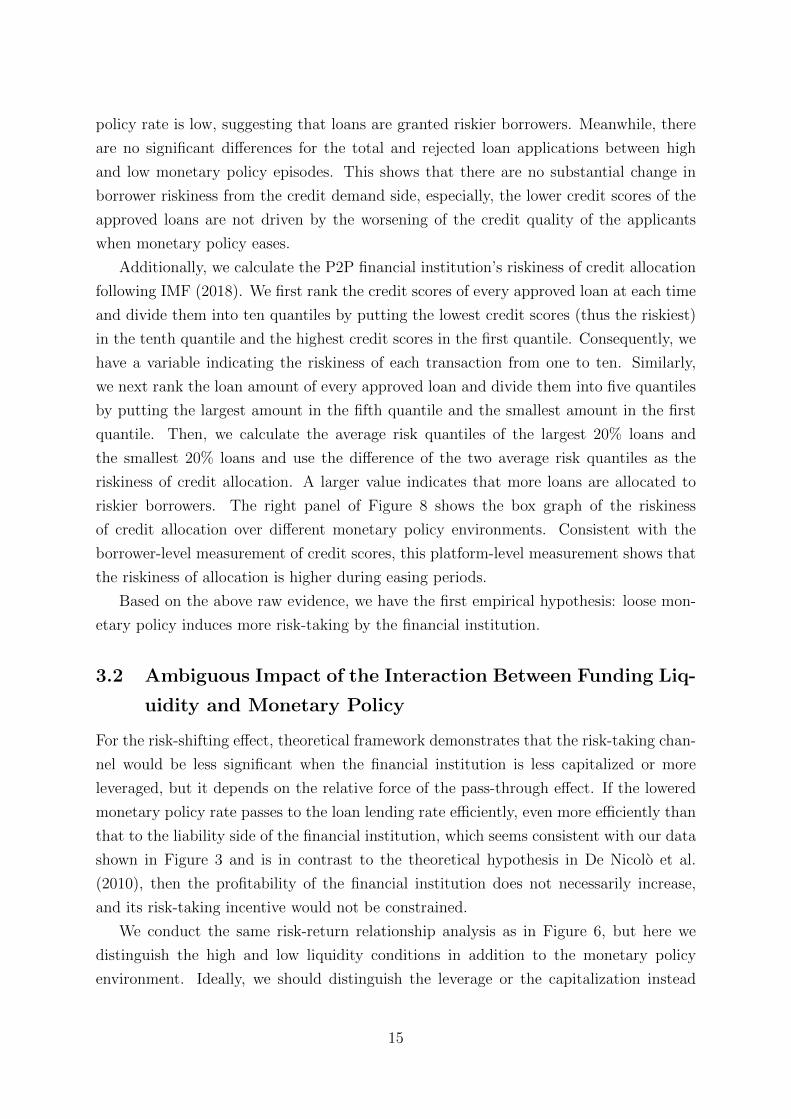
Additionally, we calculate the P2P financial institution’s riskiness of credit allocation

following IMF (2018). We first rank the credit scores of every approved loan at each time

and divide them into ten quantiles by putting the lowest credit scores (thus the riskiest)

in the tenth quantile and the highest credit scores in the first quantile. Consequently, we

have a variable indicating the riskiness of each transaction from one to ten. Similarly,

we next rank the loan amount of every approved loan and divide them into five quantiles

by putting the largest amount in the fifth quantile and the smallest amount in the first

quantile. Then, we calculate the average risk quantiles of the largest 20% loans and

the smallest 20% loans and use the difference of the two average risk quantiles as the

riskiness of credit allocation. A larger value indicates that more loans are allocated to

riskier borrowers. The right panel of Figure 8 shows the box graph of the riskiness

of credit allocation over different monetary policy environments. Consistent with the

borrower-level measurement of credit scores, this platform-level measurement shows that

the riskiness of allocation is higher during easing periods.

Based on the above raw evidence, we have the first empirical hypothesis: loose mon-

etary policy induces more risk-taking by the financial institution.

3.2 Ambiguous Impact of the Interaction Between Funding Liq-

uidity and Monetary Policy

For the risk-shifting effect, theoretical framework demonstrates that the risk-taking chan-

nel would be less significant when the financial institution is less capitalized or more

leveraged, but it depends on the relative force of the pass-through effect. If the lowered

monetary policy rate passes to the loan lending rate efficiently, even more efficiently than

that to the liability side of the financial institution, which seems consistent with our data

shown in Figure 3 and is in contrast to the theoretical hypothesis in De Nicolo et al.

(2010), then the profitability of the financial institution does not necessarily increase,

and its risk-taking incentive would not be constrained.

We conduct the same risk-return relationship analysis as in Figure 6, but here we

distinguish the high and low liquidity conditions in addition to the monetary policy

environment. Ideally, we should distinguish the leverage or the capitalization instead

15

of the liquidity. However, our dataset comes from a single P2P platform, so there is

no cross-sectional variation in capitalization, and we cannot directly observe the total

liability nor leverage. With this limitation, we attempt to make use of the liquidation

information, which is the amount of newly added funding flowing into the platform on

each day. Assuming that the platform does not alter its equity, the change in liquidity

assembles the change in leverage and the risk-shifting and pass-through story could also

apply to liquidity. Figure 9 shows that the risk-taking effect is more significant when the

financial institution has high liquidity and is insignificant during low liquidity periods.

This result is in contrast with the risk-shifting mechanism and suggests that the pass-

through effect may be stronger in this P2P platform. When monetary policy eases and

the platform has a large pool of loanable funding, its profitability is weakened because the

loan rate reduces, while the promised return to the funding inflow does not change. When

the pool of loanable funding is small, the profit pressure is lower. Therefore, the platform

has a large incentive of risk-taking when the monetary policy easing is accompanied by

high liquidity.

On the other hand, the risk-shifting mechanism depends on the limited liability pre-

sumption, which holds firmly for banks but seemingly less for nonbank financial insti-

tutions. In general, the limited liability issue should be more serious for banks than

nonbanks because the deposit insurance is only for depository-taking financial institu-

tions. The P2P lending platforms in China, however, are notorious for severe moral

hazard problems. Though they do not enjoy deposit insurance, their incentive to take

full responsibility for the investors is very low. Many P2P platforms went into prob-

lem and their heads just flew away without any thought for the investors, to whom the

platforms had promised a zero-risk repayment on the investment. This has been a social

phenomenon, especially in the early development of P2P and in the lack of proper regula-

tion by the government. Thus, the risk-shifting mechanism could be even stronger for the

P2P platforms in China, which implies that the risk-taking is stronger when monetary

policy tightens and is less when monetary policy eases.19

Thus, the role of liquidity in the risk-taking channel of monetary policy can be am-

biguous. It is also noteworthy that these figures only show raw evidence, as the liquidity

may be correlated with monetary policy. Therefore, we do not observe a clear hypothesis

here. The investigation of the interaction between liquidity and monetary policy is an

empirical question, and we leave it to Section 4.

19 This severe moral hazard problem is echoed in the figure in the appendix. Without considerationof monetary policy environment, we investigate the change in risk-taking behavior purely with liquidityconditions. The more funding it attracts from investors, the more risk-taking the P2P platform is.

16

4 Empirical Results

We employ three empirical specifications to investigate the risk-taking channel. First,

we test whether we can have similar findings in the literature using the granted loan

subsample in our dataset, as most extant studies only observe granted loans. Specifically,

we regress the riskiness measures of each granted loan on the monetary policy proxy.

Second, we employ a probit model to investigate how the probability of loans being

granted for borrowers with similar credit scores changes with monetary policy. In this

specification, both the rejected and granted loan applications are used. Finally, we use

a two-stage model with the granting of loan applications in the first stage and then the

credit amount if the loan is granted in the second stage. This specification analyzes both

the extensive and intensive margins of lending in different monetary policy environments.

4.1 Monetary Policy and the Riskiness of Granted Loans

First, we follow Dell’Ariccia et al. (2017) and Ioannidou et al. (2014) to estimate the

following specification:

Credit Scoreilt = α + βMPt−1 + γ1Loanl + γ2Borrowerit + γ3Macrot + δp + εilt (1.1)

Credit Scoreilt = α + β1MPt−1 + β2Liquidityt−1 + β3MPt−1 × Liquidityt−1+

γ1Loanl + γ2Borrowerit + γ3Macrot + δp + εilt(1.2)

where i indicates borrower, l indicates loan applications (here only the granted ones),

t indicates time, and p indicates the province location of the borrower. Credit Scoreilt

is the credit score of borrower i at the time of the loan application l. MPt−1 is one of

the monetary policy proxies as discussed in Section 2, and we use the detrended DR007

in the baseline results, while other proxies are used in robustness checks. Liquidityt−1

represents the newly added loanable funding on the liability side at time t − 1. Loanl

includes loan characteristics such as maturity, interest rate and amount. Borrowerit

includes a group of variables relating to the borrower’s mobile phone record, credit card

history and online shopping behaviors. A list of the borrower characteristics is shown in

Table 2. Macrot is a group of control variables of the macroeconomic condition, financial

market condition, and the development in the aggregate P2P industry. In particular,

it includes province-month level housing price change, country-month level change of

banking total assets and banking leverage, daily stock return for the aggregate market

and small- and medium-sized enterprises (SMEs), yield-curve, daily loan rate composite,

popularity, development and investor composite return index of the P2P industry, as well

as the monthly change in PMI and CPI.

17

We are interested in β in equation 1.1, and β1, β2 and β3 in equation 1.2. We expect

to see a positive β based on the first hypothesis, which shows that the credit scores of

granted loans decrease with a decreased monetary policy rate, indicating that the P2P

platform tends to lend to riskier borrowers when the monetary policy is eased. Based on

the second hypothesis and the raw evidence in section 3.2, we expect to see a negative β2

if the interaction term is not added, and ambiguous β1, β2 and β3 when the interaction

term is fully specified. For the estimation, we use the simple ordinary least square (OLS)

estimator. To alleviate the concern of the endogenous monetary policy, we control the

province fixed effect. As the time frequency of the loan applications is daily, we also show

the results with a month fixed effect. We cluster the standard errors at the borrower-date

level.

Table 6 presents the results for specification 1.1 and 1.2. Because the number of

borrower characteristic control variables is large and they are not our main concern in

this study, we drop the results for the borrower-level variables here for simplicity; however,

full tables are available in the online appendix. Columns (1) -(6) show the estimates with

province but without month fixed effect, and columns (7)-(12) show the estimates with

both province and month fixed effect. We add control variables gradually. Columns (1)-

(3) and Columns (7)-(9) do not analyze the role of liquidity, and the rest of the columns

account for its effect. The significant and positive coefficients of the monetary policy

is consistent with the first hypothesis and verifies the risk-taking channel of monetary

policy.

Without consideration of the interaction between liquidity and monetary policy, the

results in Table 6 show that a 100 basis points decrease in the monetary policy rate is

associated with a 4.1% decrease in the credit scores of granted borrowers. Columns (4)-(5)

and (10)-(11) show that the platform liquidity alone does not affect the riskiness of the

granted loans, especially that the monetary policy reduces the role of liquidity. Column

(6) shows that when there is no change in the monetary policy rate, a 1% increase in

platform liquidity is associated with a 0.64% increase in the credit scores of granted loans.

When the platform liquidity is average (4.31, note that here, the liquidity is rescaled by

10−3 its original value), the coefficient before detrended DR007 would be 0.038, and a one

standard deviation above the average liquidity (5.39) brings the coefficient of detrended

DR007 to 0.061. This means that the risk-taking channel is more significant when the

platform has more loanable funding. This result is consistent with the raw evidence in

Section 3.2.

When we replace the dependent variable of credit score with the borrowers’ overdue

history, the expected signs of the independent variables should be opposite. Table 7

shows the results using the number of overdue, overdue amount and the recent increase

18

in overdue number as dependent variables in estimating equations 1.1 and 1.2. The

significant and negative coefficients of monetary policy demonstrate that a lower monetary

policy rate is associated with a higher overdue history and, thus, a higher riskiness of

granted loans. However, the coefficients of the interaction term are no longer significant,

implying that liquidity does not play an important role in altering the risk-taking effect

of monetary policy.

Using the granted loan sample, we have found similar findings with existing literature

and have basically established the risk-taking channel of monetary policy.

4.2 Monetary Policy and the Loan Granting Probability

Next, we make use of the granted as well as rejected loan application entries, and investi-

gate the impact of monetary policy on the possibility of loans to be granted for borrowers

with similar credit scores or riskiness. The risk-taking channel would imply that a lower

monetary policy rate is associated with a higher probability to be granted for riskier

borrowers.

The specification is as follows, and we use a probit model to estimate it. In the two-

step analysis in section 4.3, the first stage equation is similar, but here we do not control

the borrower and time fixed effect in this probit model. In equation 2, the D(Grantedilt)

is a dummy indicating that the loan application by borrower i at time t is granted. The

other variables are interpreted in the same way as in equation 1.1 and 1.2.

D(Grantedilt) = αilt + β1MPt−1 + β2Credit Scoreilt + β3MPt−1 × Credit Scoreilt+

β4Liquidityt−1 + β5Liquidityt−1 × Credit Scoreilt + β6MPt−1 × Liquidityt−1 × Credit Scoreilt+

γ1Loanl + γ2Borrowerit + γ3Macrot + εilt

(2)

We are interested in all the six coefficients β1 to β6, but we are most interested

in β3, which is the estimate of the interaction term between monetary policy and the

credit score of the loan applicants. We expect to have a significantly negative β1 and

significantly positive β2 and β3 to verify the risk-taking channel. The interpretations are

threefold. First, a lower monetary policy rate is associated with a higher probability of

loan granting. Second, applicants with higher credit scores and lower riskiness are more

likely to be granted a loan. Third, the probability of loan granting is higher for applicants

with the same credit scores when the monetary policy rate is lower; i.e., monetary policy

easing weakens the positive relationship between credit score and loan granting.

Table 8 shows the estimates of the probit model.Similarly, we add control variables

19

gradually to see whether the results are stable. The standard errors are clustered at

the borrower-date level. The first three rows report the coefficients of monetary policy,

credit score and their interaction term. The estimates are consistent and significant

across all columns. The marginal effect after estimation shows that a one standard

deviation decrease in DR007 (0.09, or 9 bps) increases the probability of loan granting by

0.00720, a one standard deviation increase in the logarithm credit score (0.04) increases the

probability of loan granting by 0.059; and a one standard deviation decrease in liquidity

(1.08) increases the probability of loan granting by 0.002. These results show that the

most important determinant of loan granting is the credit score, and the impact of an

easing monetary policy on the higher probability of loan granting is stronger than that of a

lower liquidity. Based on the interaction term between the monetary policy and the credit

score, the results show that for a loan applicant whose credit score is low (one standard

deviation below mean, 6.41), a one standard deviation decrease in monetary policy rate

(0.09, 9 bp) increases the probability of loan granting by 0.030-0.145; however, for loan

applicants whose credit score is high(one standard deviation below mean, 6.49), the same

decrease in monetary policy rate is associated with an increase in probability of loan

granting by only as much as 0.054 or can even produce a decrease in probability by 0.053.

These results show that monetary policy easing induces the P2P platform to grant the

loan applications from riskier borrowers, and the risk-taking behavior is even stronger

for riskier borrowers. For liquidity, the results show that a standard deviation increase

in liquidity(1.08) can increase the loan granting probability for high risk borrowers by

0.012-0.120 and for low risk borrowers by -0.027-0.056. This result shows that the increase

in liquidity is associated with more risk-taking and loan granting to riskier borrowers in

particular. However, once more, the impact of liquidity is less than that of monetary

policy. Moreover, the sixth and seventh rows in Table 8 show that liquidity does not

show an impact by interacting with monetary policy.

4.3 Two-stage Selection Models for Loan Granting and Loan

Amount

In addition to the extensive margin, we are interested in the intensive margin of new lend-

ing. In particular, we ask how does loan amount change with monetary policy and does

the loan amount for riskier borrowers increase with monetary policy easing. Following

Jimenez et al. (2014), we adopt the following two-step specification.

20A 100 basis points decrease in monetary policy rate increases the probability that a loan is grantedto a borrower by 0.075 on average.

20

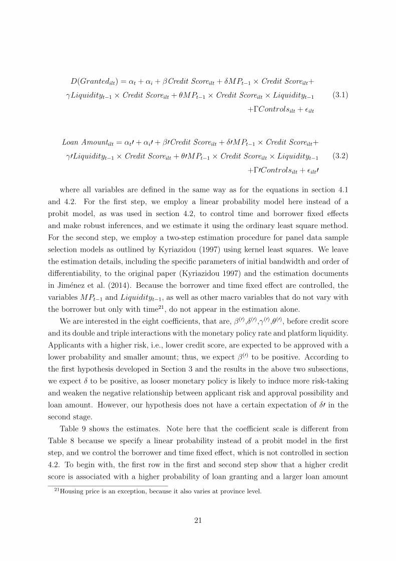
D(Grantedilt) = αt + αi + βCredit Scoreilt + δMPt−1 × Credit Scoreilt+

γLiquidityt−1 × Credit Scoreilt + θMPt−1 × Credit Scoreilt × Liquidityt−1+ΓControlsilt + εilt

(3.1)

Loan Amountilt = αt′+ αi′+ β′Credit Scoreilt + δ′MPt−1 × Credit Scoreilt+

γ′Liquidityt−1 × Credit Scoreilt + θ′MPt−1 × Credit Scoreilt × Liquidityt−1+Γ′Controlsilt + εilt′

(3.2)

where all variables are defined in the same way as for the equations in section 4.1

and 4.2. For the first step, we employ a linear probability model here instead of a

probit model, as was used in section 4.2, to control time and borrower fixed effects

and make robust inferences, and we estimate it using the ordinary least square method.

For the second step, we employ a two-step estimation procedure for panel data sample

selection models as outlined by Kyriazidou (1997) using kernel least squares. We leave

the estimation details, including the specific parameters of initial bandwidth and order of

differentiability, to the original paper (Kyriazidou 1997) and the estimation documents

in Jimenez et al. (2014). Because the borrower and time fixed effect are controlled, the

variables MPt−1 and Liquidityt−1, as well as other macro variables that do not vary with

the borrower but only with time21, do not appear in the estimation alone.

We are interested in the eight coefficients, that are, β(′),δ(′),γ(′),θ(′), before credit score

and its double and triple interactions with the monetary policy rate and platform liquidity.

Applicants with a higher risk, i.e., lower credit score, are expected to be approved with a

lower probability and smaller amount; thus, we expect β(′) to be positive. According to

the first hypothesis developed in Section 3 and the results in the above two subsections,

we expect δ to be positive, as looser monetary policy is likely to induce more risk-taking

and weaken the negative relationship between applicant risk and approval possibility and

loan amount. However, our hypothesis does not have a certain expectation of δ′ in the

second stage.

Table 9 shows the estimates. Note here that the coefficient scale is different from

Table 8 because we specify a linear probability instead of a probit model in the first

step, and we control the borrower and time fixed effect, which is not controlled in section

4.2. To begin with, the first row in the first and second step show that a higher credit

score is associated with a higher probability of loan granting and a larger loan amount

21Housing price is an exception, because it also varies at province level.

21

if the loan is granted. Next, the second row demonstrates that monetary policy plays a

significant role in altering the loan granting probability. Monetary policy rate reduction

is associated with a higher likelihood to obtain a loan for risky applicants. However,

the insignificant coefficients in the second row in the second step show that monetary

policy does not significantly affect the loan amount for risky applicants given that the

loan is granted. Combining these results, we confirm that the risk-taking channel works

in the credit quality as the loan applications from riskier borrowers are more likely to be

granted, but not necessarily in the credit quantity as the loan amount is not significantly

affected by the interaction between monetary policy and borrower riskiness. Again, there

is no robust evidence to show that platform liquidity is associated with the risk-taking

behavior in terms of loan granting probability as well as loan amount.

5 Discussion

In this section, we discuss the following four issues. First, the Chinese government

strengthened the regulation on P2P industry at the end of 2017, and we would like

to test the impact of regulation on the risk-taking channel. Second, the results so far are

based on a one-time adjustment of monetary policy, and we are interested in whether the

risk-taking effect is stronger in the periods when the monetary policy rate stays low for

a long period. Third, we would like to further alleviate the concern on loan demand by

controlling the proxy of aggregate demand. Fourth, the results above show the impact on

the probability of loan granting to risky borrowers and the loan amount when the loan

is granted; here, we construct an indicator of the riskiness of loan amount allocation to

discuss whether the risk-taking channel of monetary policy exacerbates credit allocation

quality.

5.1 The Role of Regulation

On December 1, 2017, the People’s Bank of China and the China Banking Regulatory

Commission jointly issued a strict regulation policy on internet lending with the purpose

of mitigating the risks in the P2P industry. In particular, this regulation policy aimed to

clean up controversial cash loans and the online microlending market by prohibiting loans

to people without income and placing a limit on the total charges on runaway credit. The

limits on the loan interest rate have affected the P2P industry significantly. All-in interest

rates, which include the upfront fees charged for loans, are capped by the legally allowed

annualized interest rate for loans, 36%.This upper limit may induce the P2P platforms

to lend to safer borrowers, as the riskier borrowers usually require higher interest rates.

22

Thus, we are interested in whether and how the risk-taking behavior changes with the

regulation tightening.

Tables 10 and 11 report the OLS and probit model analysis for subsamples before

and after the regulation. Table 10 shows that the risk-taking channel of monetary policy

only works before the regulation. After the regulation policy, the drop in monetary policy

rates is no longer significantly associated with the drop in credit scores of the granted loan

borrowers. Comparing the results of column (4) and column (8) in Table 11, when the

macro economic conditions are controlled in addition to loan and borrower characteristics,

we also find that the risk-taking channel disappears after the regulation. Even judging

from columns (5)-(7), where the coefficients of monetary policy and its interaction with

borrower credit scores remain significant, the scale decreases in the post-regulation period.

After the regulation, P2P platforms became more conservative, and when the mon-

etary policy rate decreases, the search-for-yield motivation is repressed for two reasons.

First, the loan rate cap makes it impossible to reach the riskiest borrowers. The willing-

ness to undertake the high risk of those borrowers is dispelled because of the regulation.

Second, compared to the previous periods without regulation, the managers now face more

administrative pressures and they have to restrict the risk-taking to yield for soundness.

These results imply that regulation, or other macro-prudential policies, is effective in

constraining the risk-taking behavior from monetary policy easing. The policymakers

can make use of the two kinds of policies together to balance growth stimulation and

financial stability.

5.2 Consecutive Loose Monetary Policy Periods

As we have found that a financial institution is more likely to lend to riskier borrowers

when the monetary policy eases, it is intuitive to predict that this risk-taking channel

might be stronger when the monetary policy is “too low for too long” (Maddaloni and

Peydro 2011). We identify the number of consecutive days of loose monetary policy

by counting the days that the detrended monetary policy rate has been continuously

negative and then repeat the OLS and probit analysis by replacing the monetary policy

rate variable with the number of consecutive days of low monetary policy. The left panel

of Figure 10 shows the predicted credit scores of approved loans when the monetary policy

has been low for k days, k = {0, 1, ...8}22, and the right panel shows the probability of

loan applications to be approved for applicants with low, mean and high credit scores

separately. The regression specifications are described in the note for Figure 10, and we

22We consider the case when monetary policy has been low as long as 8 days here. In the data, thelongest consecutive low monetary policy period lasts for 14 days, but the observations of longer than 8days are few, so we restrict the largest consecutive days of loose monetary policy to be eight.

23

report the full tables in the online appendix due to space constraints.

Figure 10 confirms the prediction that the longer the monetary policy remains loose,

the more risk-taking occurs. Generally, the riskiness of approved loans is increasing,

i.e., the credit scores of approved loan borrowers are decreasing, with the number of

consecutive days of low monetary policy. Though there are some reversals in the 3rd

to 5th day of consecutive loose monetary policy, the level of credit scores is not higher

than when monetary policy is not easing. Moreover, the probability of a risky loan

applicant(with low credit scores) being granted the loan is increasing with the length of

periods in low monetary policy, while this relationship is not obvious for borrowers with

average or low riskiness. These results suggest that the impact of low monetary policy

rates on risk-taking is amplified by relatively long and consecutive loose monetary policy

periods.

5.3 Impact of Monetary Policy on Loan Demand

The conventional analysis of monetary policy transmission suffers from the endogeneity

and simultaneity of credit demand and credit supply, as they only observe the actual

granted loans which are the outcome of changes in both demand and supply. Our data

alleviate the concern on credit demand to a large extent because we observe the borrower

profiles whose loans are granted as well as the other applications which are rejected. As

the change in credit demand is captured through the expansion or contraction of loan

applications, the change in loan granting from monetary policy is thus a pure test of

the supply side, i.e., the internet lending platform in this paper. In addition, we have

shown in Table 5 that there is no significant deterioration of loan applicant quality when

monetary policy eases. The riskiness of applicants are similar from the demand side, and

it is the supply side that drives the lower credit scores of the granted loans.

Nevertheless, we take a step further to account for the impact of monetary policy

on loan demand. Specifically, we sum up the amount of all loan applications, regardless

of being granted or not, for each day and take the natural logarithm of this value. We

use this as a proxy for loan demand in this platform. Similarly, we sum up the amount

of granted loans for each day and use its natural logarithm as a proxy of loan supply

in this platform. Then, we use the date-level data to regress the monetary policy rate

on demand proxy and supply proxy, controlling the macroeconomic conditions. Table

12 reports the results. In the control variables, the macroeconomic characters of change

in PMI, CPI, bank sector total assets and bank leverage are monthly variables instead

of daily, so they are absorbed in columns (4) and (8) when the month fixed effect is

included. The coefficients of monetary policy when the dependent variable is the demand

proxy are negative but insignificant, while the coefficients when the dependent variable is

24

the supply proxy are significantly negative, suggesting that the concern of credit demand

should not be critical in our data. These results also show that the traditional lending

channel of monetary policy also holds for this specific platform, as a monetary policy

expansion is significantly associated with an increase in loan supply. In addition, Table 12

indirectly demonstrates the interaction between banks and nonbanks, which is consistent

with the findings in Tang (2019). Specifically, the results show that the condition in

the housing and banking sector only significantly affects the demand side but not the

supply side for the P2P. Because the internet loans are not allowed to finance housing,

the increase in housing price would only increase the mortgage demand in the bank sector

and negatively relate to the credit demand in the nonbanks. The increase in the total

assets and leverage of the bank sector indicate that borrowers have more savings in the

format of bank deposits or bank lending increases, and this prosperity in bank credit is

positively related with the credit demand in the nonbank sector but not necessarily with

the credit supply in the nonbank sector.

Moreover, we add the loan demand proxy to the baseline regressions. In addition to

the daily total loan application amount, another proxy for loan demand is the number

of borrowers in the aggregate P2P market(all P2P platforms, not only the one we use in

the paper), but this variable is only available at monthly frequency. Tables 13 and 14

present the results for the OLS and probit estimations, respectively. The demand proxies

are significant in both tables and suggest that a higher demand is associated with higher

credit scores of the granted loans and lower probability of loan approval. The key results

of the risk-taking channel of monetary policy still hold when the proxies for demand are

controlled.

5.4 The Riskiness of Loan Allocation

As described in section 3.1, we calculate a proxy of the P2P platform’s riskiness of credit

allocation following IMF (2018). First, we rank the credit scores of every approved loan

on each day and divide them into ten quantiles by putting the lowest credit scores (thus,

the riskiest) in the tenth quantile and the highest credit scores in the first quantile. Thus,

we have a variable indicating the riskiness of each transaction from one to ten. Next,

we rank the loan amount of every approved loan and divide them into five quantiles

by putting the largest amount in the fifth quantile and the smallest amount in the first

quantile. Then, we calculate the average risk quantiles of the largest 20% loans and

the smallest 20% loans, and use the difference of the two average risk quantiles as the

riskiness of credit allocation. A larger value indicates that more loans are granted to

riskier borrowers.

This variable is at the platform-date level; so, we drop all the loan-level information

25

and simply regress the riskiness of loan allocation on monetary policy and other macro

variables. The results are shown in Table 15, of which the even columns have also

controlled the proxy of aggregate demand. Columns (1)-(4) show that a decrease in

monetary policy rate is associated with an increase in the riskiness of credit allocation,

i.e., more loans are allocated to riskier borrowers. Specifically, a one standard deviation

decrease in the monetary policy rate is associated with a 0.12-0.13 standard deviation

increase in the riskiness of credit allocation. Moreover, we define the easing periods as

days when the monetary policy rate is below its 25th percentile and the normal periods

as days when the rates lie within the [25th, 75th] percentile and create two dummies

for the easing periods and normal periods. Thus, the results in columns (5)-(8) show

that the riskiness of credit allocation is higher during monetary policy easing and normal

periods than tightening periods. The riskiness of credit allocation is higher by 0.38-

0.42 standard deviations during easing periods than tightening periods and by 0.35-0.42

standard deviations during normal periods than tightening periods; the impact in the

easing periods is stronger than in the normal periods.

6 Robustness Check

This section checks the robustness of the results. By using a lower frequency of monetary

policy variables, other measurements of monetary policy and conducting a placebo test,

we show that our findings for the risk-taking channel of monetary policy do not change

in quality.

6.1 Monetary Policy Measurement: Lower Frequency

First, we change the frequency of monetary policy to monthly from daily in the previous

analysis. Because there are a large number of loan applications each day in our dataset, we

are able to conduct the investigation using daily monetary policy variables. There might

be concerns that the financial institutions do not react to monetary policy change at such

a high frequency. Our response is threefold. First, the P2P platform in our dataset is also

FinTech firm; it uses algorithms and big data to monitor the applicant profile and react

to macro environment change. Thus, compared to traditional financial institutions, it

faces much less administrative obstacles and acts quickly to any policy changes. Second,

if we identify risk-taking in a high frequency, the effects should exist and be even larger

in a low frequency environment. Third, we take the average of monetary policy rates for

each month, and transform the platform liquidity to monthly variables by aggregating the

daily added liquidity. Similarly, we collapse other macro variables to a monthly frequency,

26

but the loan and borrower characteristics are still in the loan application-level.

Tables 16 and 17 report the OLS and probit estimation results. Consistent with our

conjecture, the risk-taking channel still exists based on the significant coefficients before

monthly monetary policy variables. Moreover, the scale of the coefficients is larger than

the ones in the baseline results. This result demonstrates that the P2P platform responds

to monetary policy changes by loosening the loan granting criteria and higher probability

of granting loans to riskier borrowers, and this impact is significant and stronger if the

monetary policy changes at a monthly frequency.

6.2 Other Measurements of Monetary Policy

All the results shown in the baseline analysis use the detrended DR007 to measure mon-

etary policy. Here, we first use the level of DR007 and then use other rates that are

proxies of monetary policy to replace the detrended DR007, and we find that the results

do not change in quality.

Table 18 shows the results of using level of DR007 based on all period samples,

pre-regulation and post-regulation subsamples. Again, we observe that the lower the

monetary policy rate is (level of DR007 here), the lower the credit scores. Moreover, the

risk-taking channel is stronger in the pre-regulation periods and becomes insignificant

after regulation. Table 19 shows the results using the other two price-based monetary

policy indicators, i.e., detrended R007 and shibor(1w), and the quantity based variable,

the liquidity withdraw in open market operation. The risk-taking channel conclusion is

again significantly observed when shibor(1w) and OMO liquidity are used to measure

monetary policy. Though the results based on detrended R007 are insignificant, the signs

are as expected.

6.3 Placebo Test: Longer-term Rates as Monetary Policy

As in most other countries, monetary policy targets are rates with short tenor(7-day) in

China. We replace the policy rates with longer tenor interest rates, which are not the

policy target and should not be used to measure an overnight monetary policy adjustment,

as a placebo test to check whether the risk-taking channel works through the change in

the supposititious monetary policy rates.

Thus, we select the 1-year interbank money market rates in the same series of DR007,

R007 and Shibor(1w): DR1y, R1y, Shibor(1y), as well as the ten-year government bond

yields. Tables 20 and 21 show the baseline results using these supposititious monetary

policy rates. The significance and interpretation of other loan characteristics and macroe-

conomic variables are similar to the results obtained using true monetary policy rates;

27

however, the key results of the impact of monetary policy, as reflected in the coefficients

of monetary policy and its interaction terms with credit scores, disappear. These results

are strong arguments that the measurement of monetary policy is correct in the previous

results, and the risk-taking channel does work through the easing or tightening of a true

monetary policy.

7 Conclusion

Considerable analytical effort has been expended, especially after the recent global fi-

nancial crisis, to understand the linkage between monetary policy and financial stability

through an examination of the banks’ risk-taking channels. The literature, however,

leaves the question of the financial stability implications of monetary policy in the non-

bank financial industry largely untouched. This is unsatisfactory, as nonfinancial insti-

tutions play increasingly important roles. This paper attempts to fill this gap in the

literature by examining the risk-taking consequences of a nonbank financial institution

using loan-application-level data from a P2P lending platform in China. Even in a bank-

dominated financial system such as China’s, banks do not tell the entire story. In recent

years, nonbank financial institutions, including shadow bank transactions and FinTech

platforms, have began to play greater roles. An investigation into the risk-taking behavior

of nonbank financial institutions is of great importance in deepening the understanding

of the risk-taking channel of monetary policy.

This paper represents the first academic effort to present quantitative evidence of the

risk-taking implications of monetary policy in a nonbank financial institution. Based

on the credit scores of each loan applicant, we estimate the effect of monetary policy

easing on the average credit scores of granted loans, the loan granting probability and

loan amount. In addition, we investigate the change in the risk-return relationship with

the change in monetary policy. The results confirm the search-for-yield mechanism of

monetary policy’s risk-taking channel, while we do not find consistent evidence of the

risk-shifting mechanism. We conclude that eased monetary policy is associated with

a higher probability to grant loans to risky borrowers and a greater riskiness of credit

allocation, but it does not necessarily relate to a larger loan amount on average and takes

effect through the liquidity. In addition, we also find that the introduction of the new

P2P regulation at the end of 2017 significantly reduces the risk-taking effect.

While the empirical analyses of this study use the data of a Chinese P2P platform,

the findings are of general significance and provide some important policy implications.

First, monetary policy does have important implications for financial stability. Thus,

while the monetary policy’s primary objectives should remain to achieve price stability

28

and support economic growth, monetary policymakers should also focus on the finan-

cial stability consequences. Second, an assessment of the impacts of monetary policy on

financial stability should go beyond the formal banking sector, as nonbanking financial

institutions become increasingly important. Furthermore, the risk implications could be

more significant for the generally underregulated FinTech companies. Third, macropru-

dential regulations could help mitigate the rising risks following monetary policy easing.

Consequently, while it might be difficult for the monetary policymakers to explicitly in-

corporate financial stability into their decision process, they could work more closely with

the policymakers responsible for macroprudential regulations. This consideration further

points to the advantages of the regulatory models combining both monetary policy and

macro-prudential regulations at the central bank.

Unfortunately, due to the limit of data availability, this study also suffers from some

shortcomings, which also point to important directions for future research. First, this

paper documents the risk-taking behavior of a nonbank financial institution but is not

able to compare these findings with traditional banks. It would be extremely valuable to

examine the differences of risk-taking motivations between banks and nonbank financial

institutions using comparable data. This method could help draw more reliable impli-

cations for system-wide financial stability. Second, this paper is not able to explore the

change in interest rate pricing mechanisms resulting from monetary policy changes due

to the specific loan pricing model of the financial intermediary under study. Third, as

the data ends in April 2018, we are unable to study the large-scale bankruptcy of P2P

platforms in China since June 2018, which happened under the background of tightening

liquidity and slowed-down economy growth. This could serve as the evidence of how the

accumulated risk can explode when the loose policy is gone, which backs the findings in

this paper.

29

References

Adrian, T., Estrella, A., and Shin, H. S. (2018). Risk-taking channel of monetary policy.

Financial Management.

Adrian, T. and Shin, H. S. (2008). Financial intermediaries, financial stability, and

monetary policy.

Adrian, T. and Shin, H. S. (2009). Money, liquidity, and monetary policy. American

Economic Review, 99(2):600–605.

Adrian, T. and Shin, H. S. (2010a). The changing nature of financial intermediation and

the financial crisis of 2007–2009.

Adrian, T. and Shin, H. S. (2010b). Financial intermediaries and monetary economics.

In Handbook of monetary economics, volume 3, pages 601–650. Elsevier.

Adrian, T. and Shin, H. S. (2010c). Liquidity and leverage. Journal of financial inter-

mediation, 19(3):418–437.

Altunbasa, Y., Gambacortab, L., and Marques-Ibanezc, D. (2014). Does monetary policy

affect bank risk? International Journal of Central Banking.

Angeloni, I. and Faia, E. (2009). A tale of two policies: Prudential regulation and

monetary policy with fragile banks. Technical report, Kiel working paper.

Angeloni, I. and Faia, E. (2013). Capital regulation and monetary policy with fragile

banks. Journal of Monetary Economics, 60(3):311–324.

Bekaert, G., Hoerova, M., and Duca, M. L. (2013). Risk, uncertainty and monetary

policy. Journal of Monetary Economics, 60(7):771–788.

Berger, A. N. and Udell, G. F. (2004). The institutional memory hypothesis and the

procyclicality of bank lending behavior. Journal of financial intermediation, 13(4):458–

495.

Bernanke, B. S. and Reinhart, V. R. (2004). Conducting monetary policy at very low

short-term interest rates. American Economic Review, 94(2):85–90.

BIS (2004). The 74th annual report.

Borio, C. and Zhu, H. (2012). Capital regulation, risk-taking and monetary policy: a

missing link in the transmission mechanism? Journal of Financial stability, 8(4):236–

251.

Borio, C. E. and White, W. R. (2004). Whither monetary and financial stability? the

implications of evolving policy regimes.

30

Bruno, V. and Shin, H. S. (2015). Capital flows and the risk-taking channel of monetary

policy. Journal of Monetary Economics, 71:119–132.

Buch, C. M., Eickmeier, S., and Prieto, E. (2014a). In search for yield? survey-based

evidence on bank risk taking. Journal of Economic Dynamics and Control, 43:12–30.

Buch, C. M., Eickmeier, S., and Prieto, E. (2014b). Macroeconomic factors and microlevel

bank behavior. Journal of Money, Credit and Banking, 46(4):715–751.

Burdekin, R. C. and Siklos, P. L. (2008). What has driven chinese monetary policy since

1990? investigating the people’s bank’s policy rule. Journal of International Money

and Finance, 27(5):847–859.

Cebenoyan, A. S. and Strahan, P. E. (2004). Risk management, capital structure and

lending at banks. Journal of Banking & Finance, 28(1):19–43.

Claessens, S., Frost, J., Turner, G., and Zhu, F. (2018). Fintech credit markets around

the world: size, drivers and policy issues. BIS Quarterly Review September.

De Nicolo, G., Dell’Ariccia, G., Laeven, L., and Valencia, F. (2010). Monetary policy

and bank risk taking. IMF Working Paper.

Delis, M. D., Hasan, I., and Mylonidis, N. (2017). The risk-taking channel of monetary

policy in the us: Evidence from corporate loan data. Journal of Money, Credit and

Banking, 49(1):187–213.

Delis, M. D. and Kouretas, G. P. (2011). Interest rates and bank risk-taking. Journal of

Banking & Finance, 35(4):840–855.

Dell’Ariccia, G., Laeven, L., and Suarez, G. A. (2017). Bank leverage and monetary

policy’s risk-taking channel: evidence from the united states. the Journal of Finance,

72(2):613–654.

Esty, B. C. (1998). The impact of contingent liability on commercial bank risk taking.

Journal of Financial Economics, 47(2):189–218.

Gaggl, P., Valderrama, M. T., et al. (2010). Does a low interest rate environment affect

risk taking in austria? Monetary Policy and the Economy, 4(4):32–48.

Gambacorta, L. (2009). Monetary policy and the risk-taking channel.

Gambacorta, L. and Marques-Ibanez, D. (2011). The bank lending channel: lessons from

the crisis. Economic Policy, 26(66):135–182.

Gersl, A., Jakubık, P., Kowalczyk, D., Ongena, S., and Peydro, J.-L. (2015). Mone-

tary conditions and banks’ behaviour in the czech republic. Open Economies Review,

26(3):407–445.

31

Huang, Y., Ge, T., and Wang, C. (2019). Monetary policy framework and transmission

mechanism. In Amstad, M., Sun, G., and Xiong, W., editors, Handbook of China’s

Financial System.

IMF (2018). Global financial stability report april 2018: A bumpy road ahead. Global

Financial Stability Report.

Ioannidou, V., Ongena, S., and Peydro, J.-L. (2014). Monetary policy, risk-taking, and

pricing: Evidence from a quasi-natural experiment. Review of Finance, 19(1):95–144.

Issing, O. (2003). Monetary and financial stability: is there a trade-off? BIS Papers,

18:16–23.

Jimenez, G., Ongena, S., Peydro, J.-L., and Saurina, J. (2014). Hazardous times for

monetary policy: What do twenty-three million bank loans say about the effects of

monetary policy on credit risk-taking? Econometrica, 82(2):463–505.

Kashyap, A. K. and Stein, J. C. (2000). What do a million observations on banks say

about the transmission of monetary policy? American Economic Review, 90(3):407–

428.

Khan, M. S., Scheule, H., and Wu, E. (2017). Funding liquidity and bank risk taking.

Journal of Banking & Finance, 82:203–216.

Kodres, M. L. E., Hartelius, K., and Kashiwase, K. (2008). Emerging market spread

compression: is it real or is it liquidity? Number 8-10. International Monetary Fund.

Kyriazidou, E. (1997). Estimation of a panel data sample selection model. Econometrica:

Journal of the Econometric Society, pages 1335–1364.

Laeven, L. and Levine, R. (2009). Bank governance, regulation and risk taking. Journal

of financial economics, 93(2):259–275.

Liu, L.-g. and Zhang, W. (2010). A new keynesian model for analysing monetary policy

in mainland china. Journal of Asian Economics, 21(6):540–551.

Lopez, M., Tenjo, F., and Zarate, H. (2011). The risk-taking channel and monetary trans-

mission mechanism in colombia. Ensayos sobre Polıtica Economica, 29(SPE64):212–

234.

Lopez, M., Tenjo, F., and Zarate, H. (2012). The risk-taking channelin colombia revisited.

Ensayos Sobre Polıtica Economica, 30(68):274–295.

Maddaloni, A. and Peydro, J.-L. (2011). Bank risk-taking, securitization, supervision,

and low interest rates: Evidence from the euro-area and the us lending standards. The

Review of Financial Studies, pages 2121–2165.

32

McMahon, M., Schipke, M. A., and Li, X. (2018). China’s Monetary Policy Communi-

cation: Frameworks, Impact, and Recommendations. International Monetary Fund.

Mishkin, F. S. (2011). Monetary policy strategy: lessons from the crisis. Technical report,

National Bureau of Economic Research.

Paligorova, T. and Santos, J. A. (2012). When is it less costly for risky firms to borrow?

evidence from the bank risk-taking channel of monetary policy. Technical report, Bank

of Canada Working Paper.

Rajan, R. G. (2006). Has finance made the world riskier? European Financial Manage-

ment, 12(4):499–533.

Schularick, M. and Taylor, A. M. (2012). Credit booms gone bust: Monetary policy, lever-

age cycles, and financial crises, 1870-2008. American Economic Review, 102(2):1029–61.

Smets, F. et al. (2014). Financial stability and monetary policy: How closely interlinked?

International Journal of Central Banking, 10(2):263–300.

Stein, J. C. (2012). Monetary policy as financial stability regulation. The Quarterly

Journal of Economics, 127(1):57–95.

Tang, H. (2019). Peer-to-peer lenders versus banks: substitutes or complements? The

Review of Financial Studies, 32(5):1900–1938.

Taylor, J. B. (2009). The financial crisis and the policy responses: An empirical analysis

of what went wrong. Technical report, National Bureau of Economic Research.

Valencia, F. (2014). Monetary policy, bank leverage, and financial stability. Journal of

Economic Dynamics and Control, 47:20–38.

Xiong, W. (2012). Measuring the monetary policy stance of the people’s bank of china:

An ordered probit analysis. China Economic Review, 23(3):512–533.

Zhang, W. (2009). China’s monetary policy: Quantity versus price rules. Journal of

Macroeconomics, 31(3):473–484.

33

Figures and Tables

Figure 1: Aggregated Loan Amount in the Sample and Development Index in the P2P Industry

0

2500

5000

7500

P2P

Indu

stry

Dev

elop

men

t Ind

ex

0

5

10

15

20

25

30

Gra

nted

Loa

n A

mou

nt in

the

Sam

ple(

Mill

ion

RM

B)

Aug 2017 Oct 2017 Dec 2017 Feb 2018 Apr 2018

Granted Loan Amount in the Sample P2P Industry Development Index

Note: (1) For better illustration, we transform the loan-level amount into weekly data

by aggregating the granted loan amount for each week, and taking the weekly average of

the original daily P2P industry development index. (2) The pairwise correlation of the two

series is 0.41 and significant at 1%. (3) The P2P industry development index is from WDZJ,

an information platform for the Chinese P2P industry. This index is a weighted average

of the transaction, popularity, technology, leverage, liquidity, diversity, transparency and

compliance of the P2P industry, covering every P2P platform in China. A higher value

indicates more prosperity of the industry.

34

Figure 2: Distribution of Loan Amount and Maturity in the Sample

mean

0

5

10

15

Per

cent

age

0 20000 40000 60000 80000 100000

Granted Loans, RMB

mean

0

20

40

60

Per

cent

age

6 12 18 24

Granted Loans, Months

Note: Histograms for granted loan amount and maturity. The dashed vertical line indicates

the mean value of each variable.

Figure 3: Loan Interest Rate and Investment Return in P2P

5

10

15

20

25

Inve

stor

Ret

urn/

Bor

row

er In

tere

st R

ate

(%)

01aug2017 01oct2017 01dec2017 01feb2018 01apr2018

P2P Industry Investor Composite Return Daily Average Loan Interest Rate in the Sample (%)

Note: The original data of the P2P industry investor composite return is at daily frequency

and comes from WDZJ. The the original loan interest rate is at loan-level and comes from

the specific P2P platform in this paper, and we take the average of the granted loans for

each day to generate the red line time series.

35

Figure 4: Monetary Policy

−2000

−1500

−1000

−500

0

500

1000

Net

Liq

uidi

ty W

ithdr

awl F

rom

OM

O

−1

0

1

2

3

4

5

6

7

8

Det

rend

ed M

onet

ary

Pol

icy

Rat

e

01aug2017 01oct2017 01dec2017 01feb2018 01apr2018

Detrended DR007 Detrended R007

Detrended Shibor(1w) Net Liquidity Withdrawl From OMO

Note: The Net Liquidity Withdraw from OMO is weekly data, and the detrended DR007,

R007 and Shibor(1w) are daily data.

Figure 5: Peer-to-Peer Lending in China

2017.12.10

50

100

150

200

Bill

ion

US

$

2014m1 2014m7 2015m1 2015m7 2016m1 2016m7 2017m1 2017m7 2018m4

Monthly Transaction Volume Loan Balance

2017.12.10

1000

2000

3000

4000

5000

2014m1 2014m7 2015m1 2015m7 2016m1 2016m7 2017m1 2017m7 2018m4

Number of Platform(unit) Number of Investors(thousand) Number of Borrowers(thousand)

Note: There is a P2P regulation policy announced on Dec 1, 2017. The discussion on the

regulation policy is in section 5.

36

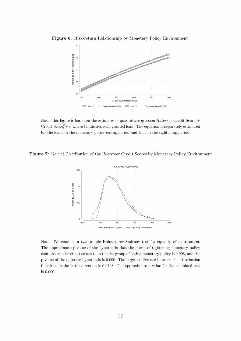
Figure 6: Risk-return Relationship by Monetary Policy Environment

10

15

20

25

30

Ann

ualiz

ed In

tere

st R

ate

(%)

600620640660680700

Credit Score (Reversed)

95% CI Easing Periods (25th) 95% CI Tightening Periods (75th)

Note: this figure is based on the estimates of quadratic regression Ratesl = Credit Scorel +

Credit Score2l +ε, where l indicates each granted loan. The equation is separately estimated

for the loans in the monetary policy easing period and that in the tightening period.

Figure 7: Kernel Distribution of the Borrower Credit Scores by Monetary Policy Environment

0

.005

.01

.015

Kde

nsity

Cre

dit S

core

550 600 650 700 750 800

Easing Periods(25th) Tightening Periods(75th)

Approved Applications

Note: We conduct a two-sample Kolmogorov-Smirnov test for equality of distribution.

The approximate p-value of the hypothesis that the group of tightening monetary policy

contains smaller credit scores than the the group of easing monetary policy is 0.998, and the

p-value of the opposite hypothesis is 0.000. The largest difference between the distribution

functions in the latter direction is 0.0728. The approximate p-value for the combined test

is 0.000.

37

Figure 8: Credit Score and Riskiness of Allocation By Monetary Policy Environment

550

600

650

700

750

Cre

dit S

core

excludes outside values

Tightening Periods(75th) Easing Periods(25th)

−4

−2

0

2

Ris

kine

ss o

f Allo

catio

n

excludes outside values

Tightening Periods (75th) Easing Periods (25th)

Note: the white line inside each box indicates the median value, and the upper hinge and

lower hinge of the box represent the 75th(q3) and 25th(q1) percentile values. he upper and

lower adjacent values are the most extreme values q3 + 1.5(q3 − q1) and q1 − 1.5(q3 − q1).

Outliers are excluded in the figures.

Figure 9: Risk-return Relationship with Monetary Policy by Liquidity Conditions

5

10

15

20

25

30

Ann

ualiz

ed In

tere

st R

ate

(%)

600620640660680700

Credit Score (Reversed)

95% CI Easing Periods (25th) 95% CI Tightening Periods (75th)

High Liquidity

5

10

15

20

25

30

Ann

ualiz

ed In

tere

st R

ate

(%)

600620640660680700

Credit Score (Reversed)

95% CI Easing Periods (25th) 95% CI Tightening Periods (75th)

Low Liquidity

Note: this figure is based on the estimates of quadratic regression Ratesl = Credit Scorel +

Credit Score2l +ε, where l indicates each granted loan. The equation is separately estimated

for the loans in the monetary policy easing period and that in the tightening period. For

the figure in the left panel, the sample is limited to high liquidity periods, defined as the

liquidity of the financial institution is above the 75th percentile. Similarly, the figure in the

right panel is that for low liquidity periods.

38

Figure 10: Consecutive Days of Low Monetary Policy

638

640

642

644

646

Pre

dict

ed C

redi

t Sco

re

0 1 2 3 4 5 6 7 8

#Days of Consecutive Low Monetary Policy

(a) Credit Scores of Approved Loans

.1

.15

.2

.25

Pro

babi

lity

of L

oan

App

rova

l

1 2 3 4 5 6 7 8

#Days of Consecutive Low Monetary Policy

Low Credit Score Mean Credit Score High Credit Score

(b) Probability of Loan Approval

Note: The left panel is based on the alternative specification of equation

1.1: Credit Scoreilt = α + βk Days in Consecutive Low Monetary Policyt−1 +

γ1Loanlt + γ2Borrowerit + γ3Macrot + δp + εilt, and the right panel is

based on the alternative specification of equation 1.2: D(Grantedilt) =

αilt + β1k Days in Consecutive Low Monetary Policyt + β2Credit Scoreilt +

β3k Days in Consecutive Low Monetary Policyt−1 × Credit Scoreilt + β4Liquidityt−1 +

β5Liquidityt−1 × Credit Scoreilt + β6k Days in Consecutive Low Monetary Policyt−1 ×Liquidityt−1 × Credit Scoreilt + γ1Loanlt + γ2Borrowerit + γ3Macrot + εilt, where we

replace the MPt−1 with k Days in Consecutive Low Monetary Policyt−1.

39

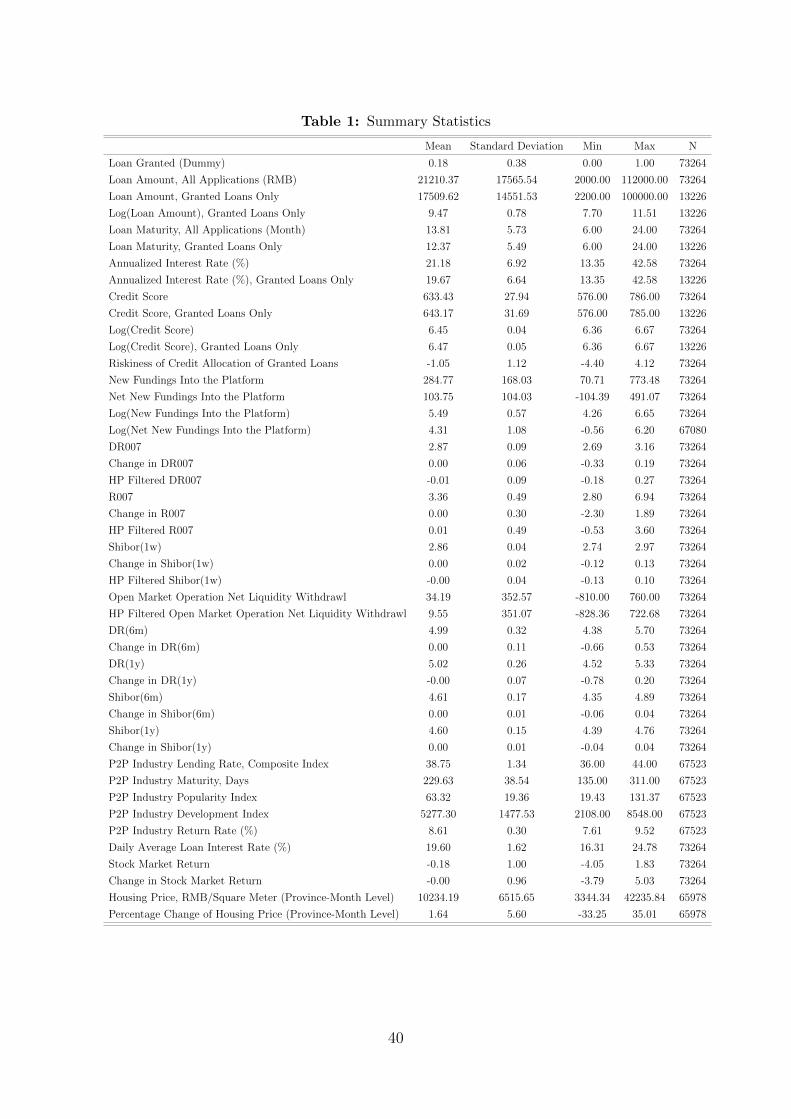
Table 1: Summary Statistics

Mean Standard Deviation Min Max N

Loan Granted (Dummy) 0.18 0.38 0.00 1.00 73264

Loan Amount, All Applications (RMB) 21210.37 17565.54 2000.00 112000.00 73264

Loan Amount, Granted Loans Only 17509.62 14551.53 2200.00 100000.00 13226

Log(Loan Amount), Granted Loans Only 9.47 0.78 7.70 11.51 13226

Loan Maturity, All Applications (Month) 13.81 5.73 6.00 24.00 73264

Loan Maturity, Granted Loans Only 12.37 5.49 6.00 24.00 13226

Annualized Interest Rate (%) 21.18 6.92 13.35 42.58 73264

Annualized Interest Rate (%), Granted Loans Only 19.67 6.64 13.35 42.58 13226

Credit Score 633.43 27.94 576.00 786.00 73264

Credit Score, Granted Loans Only 643.17 31.69 576.00 785.00 13226

Log(Credit Score) 6.45 0.04 6.36 6.67 73264

Log(Credit Score), Granted Loans Only 6.47 0.05 6.36 6.67 13226

Riskiness of Credit Allocation of Granted Loans -1.05 1.12 -4.40 4.12 73264

New Fundings Into the Platform 284.77 168.03 70.71 773.48 73264

Net New Fundings Into the Platform 103.75 104.03 -104.39 491.07 73264

Log(New Fundings Into the Platform) 5.49 0.57 4.26 6.65 73264

Log(Net New Fundings Into the Platform) 4.31 1.08 -0.56 6.20 67080

DR007 2.87 0.09 2.69 3.16 73264

Change in DR007 0.00 0.06 -0.33 0.19 73264

HP Filtered DR007 -0.01 0.09 -0.18 0.27 73264

R007 3.36 0.49 2.80 6.94 73264

Change in R007 0.00 0.30 -2.30 1.89 73264

HP Filtered R007 0.01 0.49 -0.53 3.60 73264

Shibor(1w) 2.86 0.04 2.74 2.97 73264

Change in Shibor(1w) 0.00 0.02 -0.12 0.13 73264

HP Filtered Shibor(1w) -0.00 0.04 -0.13 0.10 73264

Open Market Operation Net Liquidity Withdrawl 34.19 352.57 -810.00 760.00 73264

HP Filtered Open Market Operation Net Liquidity Withdrawl 9.55 351.07 -828.36 722.68 73264

DR(6m) 4.99 0.32 4.38 5.70 73264

Change in DR(6m) 0.00 0.11 -0.66 0.53 73264

DR(1y) 5.02 0.26 4.52 5.33 73264

Change in DR(1y) -0.00 0.07 -0.78 0.20 73264

Shibor(6m) 4.61 0.17 4.35 4.89 73264

Change in Shibor(6m) 0.00 0.01 -0.06 0.04 73264

Shibor(1y) 4.60 0.15 4.39 4.76 73264

Change in Shibor(1y) 0.00 0.01 -0.04 0.04 73264

P2P Industry Lending Rate, Composite Index 38.75 1.34 36.00 44.00 67523

P2P Industry Maturity, Days 229.63 38.54 135.00 311.00 67523

P2P Industry Popularity Index 63.32 19.36 19.43 131.37 67523

P2P Industry Development Index 5277.30 1477.53 2108.00 8548.00 67523

P2P Industry Return Rate (%) 8.61 0.30 7.61 9.52 67523

Daily Average Loan Interest Rate (%) 19.60 1.62 16.31 24.78 73264

Stock Market Return -0.18 1.00 -4.05 1.83 73264

Change in Stock Market Return -0.00 0.96 -3.79 5.03 73264

Housing Price, RMB/Square Meter (Province-Month Level) 10234.19 6515.65 3344.34 42235.84 65978

Percentage Change of Housing Price (Province-Month Level) 1.64 5.60 -33.25 35.01 65978

40

Table 2: Summary Statistics of Borrower Characteristics

Mean Standard Deviation Min Max N

Male 0.72 0.45 0.00 1.00 73264

Age 32.83 6.39 19.00 63.00 73264

Number of Mobile Phone Carriers 1.22 0.96 0.00 31.00 73264

Number of calls In the Past 3 Months 1076.63 977.75 0.00 19553.00 73264

Longest Call Duration In The Past 12 Months 153.62 9490.74 0.00 592177.05 73264

Ratio of Frequent Calls In Contact Book In the Past 12 Months 0.66 0.26 0.00 1.00 73264

Number of Calls In the Black List In the Past 12 Months 0.02 1.62 0.00 205.00 73264

Number of Calls With Family In the Past 12 Months 382.16 646.29 0.00 9592.00 73264

Number of Calls With Agents As Caller 23.88 90.18 0.00 2973.00 73264

Number of Calls In the Past 3 Months As Caller 495.03 498.10 0.00 9473.00 73264

Longest Call Duration In The Past 12 Months As Caller 2277.36 1789.95 0.00 21710.00 73264

Median Call Duration In The Past 12 Months As Caller 43.61 20.98 0.00 816.00 73264

Number of Calls To Agents in the Past 12 Months As Caller 7.33 38.80 0.00 2450.00 73264

Number of Calls In the Black List In the Past 12 Months 0.02 1.25 0.00 155.00 73264

Ratio of Calls In Contact Book In the Past 12 Months As Caller 0.69 0.25 0.00 1.00 73264

Average Times of Being Called Per Day In the Past 12 Months 6.80 5.89 0.00 125.01 73264

Average Times of Being Caller Per Day In the Past 12 Months 5.91 5.53 0.00 84.04 73264

Average Mobile Bill In the Past 12 Months 94.01 129.88 0.00 6791.28 73264

Have Shortcuts for Family In the Past 12 Months 0.12 0.33 0.00 1.00 73264

Number of the Contacts In The Contact Book 672.15 888.01 0.00 31937.00 73264

Transaction Amount With Trading Companies In The Past 12 Months 77579.00 205767.79 0.00 6403776.00 73264

Transaction Number With Trading Companies In The Past 12 Months 12.45 26.02 0.00 671.00 73264

Number of Active Credit Cards 6.49 5.00 0.00 163.00 73264

Number of Banks of the Credit Cards 5.09 2.77 0.00 18.00 73264

Number of Cash Withdrawal in the Past 12 Months 10.76 35.81 0.00 1493.00 73264

Total Interest Charged In the Past 6 Months 4070.36 7637.09 0.00 154375.94 73264

Number of Interest Charged In the Past 12 Months 33.12 45.42 0.00 1317.00 73264

Number of Transactions Over 5000 RMB in the Past 12 Months 55.88 108.20 0.00 5766.00 73264

Highest Credit Line in the Past 12 Months 43522.03 39869.76 0.00 512488.74 73264

Repayment Rate in the Past 6 Months 0.68 0.33 0.00 1.00 73264

Minimum Repayment Rate in the Past 12 Months 0.42 0.39 0.00 1.00 73264

Usage Rate of Credit Line in the Past 6 Months 0.62 0.23 0.00 1.00 73264

Number Of Bank Relationship In The Past 3 Months 0.77 0.70 0.00 7.00 73264

Number Of Active Deposit Cards In The Past 3 Months 0.91 0.93 0.00 11.00 73264

Average Transfer Per Day In the Past 12 Months 312.42 983.04 0.00 25462.97 73264

Alipay Implied Credit Lines In The Past 12 Months 2279.37 9311.71 0.00 174100.00 73264

Alipay Implied Number of Banks of Credit Cards In The Past 12 Months 0.36 1.01 0.00 11.00 73264

Alipay Implied Highest Credit Line In The Past 12 Months 1314.59 4434.50 0.00 50000.00 73264

Alipay Implied Average Income Per Day In The Past 12 Months 210.28 715.48 0.00 27011.63 73264

41

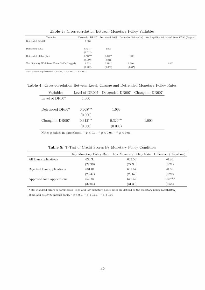
Table 3: Cross-correlation Between Monetary Policy Variables

Variables Detrended DR007 Detrended R007 Detrended Shibor(1w) Net Liquidity Withdrawl From OMO (Lagged)

Detrended DR007 1.000

Detrended R007 0.421∗∗ 1.000

(0.012)

Detrended Shibor(1w) 0.747∗∗∗ 0.347∗∗ 1.000

(0.000) (0.041)

Net Liquidity Withdrawl From OMO (Lagged) 0.232 0.384∗∗ 0.300∗ 1.000

(0.202) (0.030) (0.095)

Note: p-values in parentheses. ∗ p < 0.1, ∗∗ p < 0.05, ∗∗∗ p < 0.01.

Table 4: Cross-correlation Between Level, Change and Detrended Monetary Policy Rates

Variables Level of DR007 Detrended DR007 Change in DR007

Level of DR007 1.000

Detrended DR007 0.968∗∗∗ 1.000

(0.000)

Change in DR007 0.312∗∗∗ 0.329∗∗∗ 1.000

(0.000) (0.000)

Note: p-values in parentheses. ∗ p < 0.1, ∗∗ p < 0.05, ∗∗∗ p < 0.01.

Table 5: T-Test of Credit Scores By Monetary Policy Condition

High Monetary Policy Rate Low Monetary Policy Rate Difference (High-Low)

All loan applications 633.30 633.56 -0.26

(27.99) (27.90) (0.21)

Rejected loan applications 631.01 631.57 -0.56

(26.47) (26.67) (0.22)

Approved loan applications 643.84 642.52 1.32***

(32.04) (31.33) (0.55)

Note: standard errors in parentheses. High and low monetary policy rates are defined as the monetary policy rate(DR007)

above and below its median value. ∗ p < 0.1, ∗∗ p < 0.05, ∗∗∗ p < 0.01

42

Table 6: Monetary Policy Rates and Credit Scores of Granted Loans

This table shows the results from regressing the credit score of approved loan applications on monetary policy, the liquidity

of the platform, i.e. newly added loanable funding, the interaction between monetary policy and platform liquidity, and

a vector of control variables of the loan, borrower and macroeconomic conditions. Province and month fixed effects are

controlled in respective columns. We use the sample of approved loan applications and employ OLS estimation for this

table. The estimates for borrower characteristics are omitted here due to space limit. Standard errors are clustered at the

borrower and date levels.

(1) (2) (3) (4) (5) (6) (7) (8) (9) (10) (11) (12)

Ln(Credit Score) Ln(Credit Score) Ln(Credit Score) Ln(Credit Score) Ln(Credit Score) Ln(Credit Score) Ln(Credit Score) Ln(Credit Score) Ln(Credit Score) Ln(Credit Score) Ln(Credit Score) Ln(Credit Score)

Lagged Detrended DR007 0.04∗∗∗ 0.04∗∗∗ 0.04∗∗∗ 0.04∗∗∗ -0.05∗∗∗ 0.02∗∗∗ 0.01∗∗∗ 0.02∗∗∗ 0.02∗∗∗ -0.03∗∗

(0.000) (0.000) (0.000) (0.000) (0.001) (0.000) (0.000) (0.000) (0.000) (0.030)

Log Lagged Liquidity -0.39 -0.29 0.64∗ -0.19 -0.10 0.43

(0.213) (0.367) (0.072) (0.530) (0.748) (0.216)

Lagged Detrended DR007 × Log Lagged Liquidity 20.54∗∗∗ 11.47∗∗∗

(0.000) (0.000)

Log Loan Amount 0.22 1.27∗∗∗ 1.35∗∗∗ 1.23∗∗∗ 1.21∗∗∗ 0.90∗∗ 0.86∗∗ 0.87∗∗ 0.86∗∗ 0.85∗∗

(0.607) (0.002) (0.002) (0.005) (0.006) (0.019) (0.031) (0.039) (0.043) (0.043)

Loan Maturity -1.67∗∗∗ -1.82∗∗∗ -1.82∗∗∗ -1.81∗∗∗ -1.81∗∗∗ -1.82∗∗∗ -1.87∗∗∗ -1.87∗∗∗ -1.86∗∗∗ -1.86∗∗∗

(0.000) (0.000) (0.000) (0.000) (0.000) (0.000) (0.000) (0.000) (0.000) (0.000)

Loan Interest Rate -0.01∗∗∗ -0.01∗∗∗ -0.01∗∗∗ -0.01∗∗∗ -0.01∗∗∗ -0.01∗∗∗ -0.01∗∗∗ -0.01∗∗∗ -0.01∗∗∗ -0.01∗∗∗

(0.000) (0.000) (0.000) (0.000) (0.000) (0.000) (0.000) (0.000) (0.000) (0.000)

Lagged Stock Market Return 0.04 -0.54 -0.20 -0.50 -0.54 -0.79 -0.62 -0.77

(0.940) (0.306) (0.704) (0.343) (0.281) (0.124) (0.229) (0.135)

Lagged Stock Market Return for SMEs -0.30 0.66∗ -0.35 -0.08 0.14 0.64∗ 0.11 0.24

(0.413) (0.065) (0.351) (0.834) (0.699) (0.072) (0.764) (0.515)

Lagged Yield Curve 0.02∗∗∗ 0.02∗∗∗ 0.02∗∗∗ 0.02∗∗∗ 0.01∗∗∗ 0.00 0.01∗∗∗ 0.01∗∗

(0.000) (0.000) (0.000) (0.000) (0.003) (0.313) (0.005) (0.015)

P2P Industry Loan Rate Composite Index 0.70∗ 2.44∗∗∗ 1.43∗∗∗ 1.52∗∗∗ 0.58 1.33∗∗∗ 0.82∗ 0.90∗∗

(0.061) (0.000) (0.001) (0.000) (0.131) (0.002) (0.055) (0.037)

P2P Industry Popularity Index 0.08∗∗∗ 0.10∗∗∗ 0.08∗∗∗ 0.07∗∗∗ 0.03∗ 0.04∗∗ 0.03∗ 0.03

(0.000) (0.000) (0.000) (0.001) (0.056) (0.022) (0.074) (0.169)

P2P Industry Investor Composite Return 0.65 0.86 -1.06 -0.67 -2.06 -2.20 -2.57 -2.43

(0.695) (0.624) (0.547) (0.704) (0.222) (0.226) (0.156) (0.178)

Lagged Change in Housing Price -0.20∗∗ -0.13 -0.17∗∗ -0.15∗ -0.14 -0.12 -0.13 -0.13

(0.014) (0.102) (0.044) (0.060) (0.117) (0.168) (0.156) (0.153)

Lagged Change in Banking Total Assets 0.05∗∗∗ 0.05∗∗∗ 0.05∗∗∗ 0.05∗∗∗

(0.000) (0.000) (0.000) (0.000)

Lagged Change in Banking Leverage -0.25∗∗∗ -0.28∗∗∗ -0.27∗∗∗ -0.28∗∗∗

(0.000) (0.000) (0.000) (0.000)

Lagged Change in PMI -0.01∗∗∗ -0.01∗∗∗ -0.01∗∗∗ -0.01∗∗∗

(0.000) (0.000) (0.000) (0.000)

Lagged Change in CPI -0.02∗∗∗ -0.02∗∗∗ -0.02∗∗∗ -0.02∗∗∗

(0.000) (0.000) (0.000) (0.000)

Constant 6.47∗∗∗ 6.55∗∗∗ 6.44∗∗∗ 6.37∗∗∗ 6.43∗∗∗ 6.41∗∗∗ 6.47∗∗∗ 6.56∗∗∗ 6.56∗∗∗ 6.53∗∗∗ 6.56∗∗∗ 6.55∗∗∗

(0.000) (0.000) (0.000) (0.000) (0.000) (0.000) (0.000) (0.000) (0.000) (0.000) (0.000) (0.000)

Observations 11956 11956 10953 10008 9922 9922 11956 11956 10953 10008 9922 9922

Adjusted R-Squared 0.02 0.59 0.66 0.65 0.66 0.66 0.12 0.68 0.69 0.69 0.68 0.68

Loan Characteristics NO YES YES YES YES YES NO YES YES YES YES YES

Borrower Characteristics NO YES YES YES YES YES NO YES YES YES YES YES

Macro Characteristics NO NO YES YES YES YES NO NO YES YES YES YES

Borrower Province FE YES YES YES YES YES YES YES YES YES YES YES YES

Month FE NO NO NO NO NO NO YES YES YES YES YES YES

p-values in parentheses

In this table the independent variable of Log Lagged Liquidity, Log Loan Amount, Loan Maturity, Lagged Stock Market Return, Lagged Stock Market Return for SMES,

P2P Industry Loan Rate Composite Index, P2P Industry Popularity Index, P2P Industry Investor Composite Return, Lagged Change in Housing Price and Lagged CHange in Banking Total Assets are rescaled by 10−3 times original value, for clear presentation of the estimates.

∗ p < 0.1, ∗∗ p < 0.05, ∗∗∗ p < 0.01

43

Table 7: Monetary Policy Rates and Riskiness of Granted Loans

This table shows the results from regressing the riskiness of approved loan applications, which is proxied by the number of

overdue in the past 6 months in columns(1)-(3), the amount of overdue in the past 6 months in columns (4)-(6), the ratio

of overdue number in the past 3 month to that in the past 9 month in columns(7)-(9), on monetary policy, the liquidity

of the platform, i.e. newly added loanable funding, the interaction between monetary policy and platform liquidity, and

a vector of control variables of the loan, borrower and macroeconomic conditions. Province and month fixed effects are

controlled. We use the sample of approved loan applications and employ OLS estimation for this table. The estimates for

borrower characteristics are omitted here due to space limit. Standard errors are clustered at the borrower and date levels.

Number of Overdue(6M) Amount of Overdue(6M) Number of Overdue Ratio(3M to 9M)

(1) (2) (3) (4) (5) (6) (7) (8) (9)

Lagged Detrended DR007 -367.26∗∗∗ -353.93∗∗∗ -874.39∗ -52.89∗ -47.53 -182.52∗ -685.49∗∗∗ -712.15∗∗∗ -1692.12

(0.002) (0.006) (0.059) (0.068) (0.133) (0.053) (0.006) (0.008) (0.129)

Log Lagged Liquidity 16.95∗ 22.37∗∗ 3.22∗∗ 4.63∗∗∗ -14.10 -3.90

(0.091) (0.046) (0.047) (0.009) (0.583) (0.881)

Lagged Detrended DR007 × Log Lagged Liquidity 117.39 30.45 221.04

(0.247) (0.102) (0.358)

Log Loan Amount 42.45∗∗∗ 41.34∗∗ 41.32∗∗ 11.92∗∗∗ 12.24∗∗∗ 12.24∗∗∗ 8.07 6.82 6.78

(0.007) (0.017) (0.017) (0.002) (0.005) (0.005) (0.747) (0.800) (0.801)

Loan Maturity 3.71∗∗ 4.29∗∗ 4.29∗∗ -0.10 -0.02 -0.02 -1.32 -1.29 -1.29

(0.040) (0.027) (0.027) (0.804) (0.963) (0.964) (0.720) (0.745) (0.745)

Loan Interest Rate 3.30∗∗ 3.11∗∗ 3.11∗∗ 0.45 0.45 0.45 0.74 0.48 0.48

(0.019) (0.032) (0.033) (0.110) (0.121) (0.122) (0.798) (0.873) (0.875)

Lagged Stock Market Return -4.82 -2.00 -3.54 1.50 2.51 2.10 33.97 26.40 23.49

(0.792) (0.915) (0.851) (0.625) (0.432) (0.511) (0.253) (0.389) (0.450)

Lagged Stock Market Return for SMEs 35.38∗∗ 31.42∗∗ 32.78∗∗ 6.31∗∗ 5.84∗∗ 6.19∗∗ 19.54 22.98 25.53

(0.014) (0.032) (0.026) (0.018) (0.035) (0.027) (0.338) (0.270) (0.230)

Lagged Yield Curve -45.08 -32.16 -42.39 -22.03 -19.85 -22.50 -218.59 -258.28 -277.54

(0.623) (0.746) (0.673) (0.217) (0.309) (0.255) (0.216) (0.175) (0.151)

P2P Industry Loan Rate Composite Index 7.68 14.79 15.57 3.56 3.83 4.03 21.50 48.01 49.46

(0.468) (0.263) (0.242) (0.121) (0.181) (0.157) (0.367) (0.115) (0.104)

P2P Industry Popularity Index -0.50 -0.64 -0.72 -0.10 -0.14 -0.16 -1.01 -0.45 -0.59

(0.342) (0.255) (0.204) (0.351) (0.203) (0.145) (0.364) (0.708) (0.621)

P2P Industry Investor Composite Return -37.28 -53.57 -52.14 -21.72∗ -23.11∗ -22.74∗ -107.05 -164.49 -161.81

(0.457) (0.334) (0.347) (0.070) (0.084) (0.090) (0.368) (0.224) (0.233)

Lagged Change in Housing Price 0.99 1.68 1.68 -0.75 -0.75 -0.75 4.47 3.19 3.18

(0.760) (0.611) (0.613) (0.393) (0.402) (0.401) (0.274) (0.446) (0.448)

Constant -272.46 -419.54 -485.81 -41.90 -48.96 -66.15 1082.60 580.47 455.69

(0.552) (0.399) (0.343) (0.673) (0.644) (0.548) (0.217) (0.540) (0.638)

Observations 10953 9922 9922 10953 9922 9922 10953 9922 9922

Adjusted R-Squared 0.03 0.03 0.03 0.06 0.07 0.07 0.01 0.01 0.01

Loan Characteristics YES YES YES YES YES YES YES YES YES

Borrower Characteristics YES YES YES YES YES YES YES YES YES

Macro Characteristics YES YES YES YES YES YES YES YES YES

Province FE YES YES YES YES YES YES YES YES YES

Month FE YES YES YES YES YES YES YES YES YES

p-values in parentheses

In this table the dependent variable of Number of Overdue (6M) and Number of Overdue Ratio(3M to 9M) are rescaled by 1000 times original value, for clear presentation of the estimates.

∗ p < 0.1, ∗∗ p < 0.05, ∗∗∗ p < 0.01

44

Table 8: Monetary Policy and Loan Granting Probability:Credit Score of Loan Applicants

This table shows the results from the Probit estimation of loan granting on monetary policy, the credit score of the loan

applicant, the liquidity of the platform, i.e. newly added loanable funding, the full interaction terms between these three

variables, and a vector of control variables of the loan, borrower and macroeconomic conditions. No fixed effects are

controlled in this probit estimation, but will be controlled in the next two-step analysis. The estimates for borrower

characteristics are omitted here due to space limit. Standard errors are clustered at the borrower and date levels.

(1) (2) (3) (4) (5) (6) (7)

Granted Granted Granted Granted Granted Granted Granted

Granted

Lagged Detrended DR007 -0.14∗∗ -36.30∗∗∗ -93.67∗∗ -83.15∗ -87.73∗∗ -74.95∗

(0.026) (0.000) (0.027) (0.051) (0.041) (0.085)

Ln(Credit Score) 5.33∗∗∗ 8.56∗∗∗ 8.76∗∗∗ 8.38∗∗∗ 7.80∗∗∗ 8.15∗∗∗

(0.000) (0.000) (0.000) (0.000) (0.000) (0.000)

Lagged Detrended DR007 × Ln(Credit Score) 5.58∗∗∗ 14.37∗∗ 12.72∗ 13.44∗∗ 11.64∗

(0.000) (0.028) (0.054) (0.043) (0.084)

Lagged Liquidity 4.65∗∗∗ 4.79∗∗∗ 4.84∗∗∗ 4.36∗∗∗ 2.96∗∗∗

(0.000) (0.000) (0.000) (0.000) (0.001)

Lagged Liquidity × Ln(Credit Score) -0.71∗∗∗ -0.73∗∗∗ -0.74∗∗∗ -0.67∗∗∗ -0.46∗∗∗

(0.000) (0.000) (0.000) (0.000) (0.001)

Lagged Detrended DR007 × Lagged Liquidity 13.48 10.92 12.90 14.32

(0.150) (0.248) (0.175) (0.137)

Lagged Detrended DR007 × Ln(Credit Score) × Lagged Liquidity -2.07 -1.67 -1.97 -2.24

(0.154) (0.255) (0.180) (0.134)

Log Loan Amount -0.19∗∗∗ -0.25∗∗∗ -0.27∗∗∗

(0.000) (0.000) (0.000)

Loan Maturity -0.03∗∗∗ -0.03∗∗∗ -0.02∗∗∗

(0.000) (0.000) (0.000)

Loan Interest Rate -0.01∗∗∗ -0.01∗∗∗ -0.01∗∗∗

(0.000) (0.000) (0.001)

Lagged Change in Housing Price 0.01∗∗∗

(0.001)

Lagged Change in Banking Total Assets -0.00∗∗∗

(0.000)

Lagged Change in Banking Leverage 3.45∗∗∗

(0.000)

Lagged Stock Market Return -0.04∗∗∗

(0.000)

Lagged Stock Market Return for SMEs 0.01∗

(0.092)

Lagged Yield Curve 0.06

(0.217)

P2P Industry Loan Rate Composite Index -0.02∗

(0.077)

P2P Industry Popularity Index 0.00

(0.167)

P2P Industry Investor Composite Return 0.01

(0.725)

Lagged Change in PMI 0.21∗∗∗

(0.000)

Lagged Change in CPI 0.46∗∗∗

(0.000)

Constant -0.92∗∗∗ -35.32∗∗∗ -56.49∗∗∗ -57.76∗∗∗ -53.02∗∗∗ -48.85∗∗∗ -49.29∗∗∗

(0.000) (0.000) (0.000) (0.000) (0.000) (0.000) (0.000)

Observations 72861 72861 66639 66236 66236 66236 54113

Loan Characteristics NO NO NO NO YES YES YES

Borrower Characteristics NO NO NO NO NO YES YES

Macro Characteristics NO NO NO NO NO NO YES

Borrower FE NO NO NO NO NO NO NO

Time FE NO NO NO NO NO NO NO

p-values in parentheses

∗ p < 0.1, ∗∗ p < 0.05, ∗∗∗ p < 0.01

45

Table 9: Two-Step Model: Loan Granting and Amount

This table shows the results from the two-stage estimation. The first stage employs a linear probability model, by regressing

loan granting on monetary policy, the credit score of the loan applicant, the liquidity of the platform, i.e. newly added

loanable funding, the full interaction terms between these three variables, and a vector of control variables of the loan,

borrower and macroeconomic conditions. Borrower and date fixed effects are controlled. The dependent variable in the

second-stage is the amount of granted loans. For the second step, we employ a two-step estimation procedure for panel

data sample selection models as outlined by Kyriazidou (1997) using kernel least squares. We leave the estimation details,

including the specific parameters of initial bandwidth and order of differentiability, to the original paper (Kyriazidou 1997)

and the estimation documents in Jimenez et al. (2014). Because the borrower and time fixed effect are controlled, the

variables monetary policy and platform liquidity, as well as other macro variables that do not vary with the borrower but

only with time do not appear in the estimation alone. The estimates for loan characteristics, borrower characteristics and

macroeconomic conditions are omitted here due to space limit. Standard errors are clustered at the borrower and date

levels.

(1) (2) (3) (4) (5) (6) (7) (8)

First Step: Granted

Ln(Credit Score) 0.602∗∗∗ 0.594∗∗∗ 0.591∗∗∗ 0.584∗∗∗ 0.372∗∗∗ 0.359∗∗∗ 0.381∗∗∗ 0.367∗∗∗

(0.000) (0.000) (0.000) (0.000) (0.000) (0.000) (0.000) (0.000)

Ln(Credit Score) × Lagged Detrended DR007 0.167∗∗∗ 0.176∗∗∗ 0.115∗ 0.128∗∗

(0.000) (0.005) (0.051) (0.039)

Ln(Credit Score) × Lagged Liquidity 0.002∗ 0.002∗ 0.002 0.002

(0.069) (0.092) (0.103) (0.129)

Ln(Credit Score) × Lagged Liquidity × Lagged Detrended DR007 -0.004∗ -0.003

(0.096) (0.325)

Observations 73264 72861 66639 66236 65978 65616 60091 59729

Borrower FE Yes Yes Yes Yes Yes Yes Yes Yes

Date FE Yes Yes Yes Yes Yes Yes Yes Yes

Loan Controls No No No No Yes Yes Yes Yes

Borrower Controls No No No No Yes Yes Yes Yes

Macroeconomic Controls No No No No Yes Yes Yes Yes

Second Step: Loan Amount

Ln(Credit Score) 1.513∗∗∗ 1.518∗∗∗ 1.528∗∗∗ 1.532∗∗∗ 0.910∗∗ 0.899∗∗ 0.886∗∗ 0.870∗∗

(0.000) (0.000) (0.000) (0.000) (0.013) (0.014) (0.016) (0.018)

Ln(Credit Score) × Lagged Detrended DR007 -0.095 -0.179 -0.210 -0.333

(0.744) (0.568) (0.557) (0.374)

Ln(Credit Score) × Lagged Liquidity -0.003 -0.003 -0.004 -0.004

(0.521) (0.558) (0.386) (0.415)

Ln(Credit Score) × Lagged Liquidity × Lagged Detrended DR007 0.020 0.020

(0.295) (0.282)

Observations 13226 13130 12085 11989 12042 11956 11011 10925

Borrower FE Yes Yes Yes Yes Yes Yes Yes Yes

Date FE Yes Yes Yes Yes Yes Yes Yes Yes

Loan Controls No No No No Yes Yes Yes Yes

Borrower Controls No No No No Yes Yes Yes Yes

Macroeconomic Controls No No No No Yes Yes Yes Yes

p-values in parentheses

∗ p < 0.1, ∗∗ p < 0.05, ∗∗∗ p < 0.01

46

Table 10: Granted Loan Only: Before and After Regulation

This table shows the results from regressing the credit score of approved loan applications on monetary policy, the liquidity

of the platform, i.e. newly added loanable funding, the interaction between monetary policy and platform liquidity, and

a vector of control variables of the loan, borrower and macroeconomic conditions. Province and month fixed effects are

controlled in respective columns. We use the sample of approved loan applications and employ OLS estimation for this

table. Columns(1)-(3) use the subsample before the regulation policy in December 2017, and columns(4)-(6) use the post-

regulation subsample. The estimates for borrower characteristics are omitted here due to space limit. Standard errors are

clustered at the borrower and date levels.

Before Regulation After Regulation

(1) (2) (3) (4) (5) (6)

Ln(Credit Score) Ln(Credit Score) Ln(Credit Score) Ln(Credit Score) Ln(Credit Score) Ln(Credit Score)

Lagged Detrended DR007 0.04∗∗∗ 0.04∗∗∗ -0.05∗ -0.00 -0.00 0.01

(0.000) (0.000) (0.062) (0.697) (0.761) (0.686)

Log Lagged Liquidity -0.04 1.43∗∗ -0.46 -0.52

(0.929) (0.021) (0.321) (0.279)

Lagged Detrended DR007 × Log Lagged Liquidity 17.16∗∗∗ -2.86

(0.000) (0.622)

Log Loan Amount 0.63 0.50 0.52 1.08∗ 1.17∗ 1.17∗

(0.250) (0.391) (0.372) (0.057) (0.055) (0.054)

Loan Maturity -1.96∗∗∗ -1.95∗∗∗ -1.95∗∗∗ -1.82∗∗∗ -1.82∗∗∗ -1.82∗∗∗

(0.000) (0.000) (0.000) (0.000) (0.000) (0.000)

Loan Interest Rate -0.01∗∗∗ -0.01∗∗∗ -0.01∗∗∗ -0.01∗∗∗ -0.01∗∗∗ -0.01∗∗∗

(0.000) (0.000) (0.000) (0.000) (0.000) (0.000)

Lagged Stock Market Return 0.00 0.10 -0.47 -0.49 -0.57 -0.53

(1.000) (0.951) (0.764) (0.376) (0.335) (0.386)

Lagged Stock Market Return for SMEs -1.88∗ -2.16∗ -1.91∗ 1.06∗∗∗ 1.15∗∗∗ 1.12∗∗∗

(0.091) (0.057) (0.093) (0.009) (0.006) (0.008)

Lagged Yield Curve 0.02∗∗∗ 0.01∗∗∗ 0.01∗∗ 0.01∗∗ 0.01∗ 0.01∗

(0.000) (0.002) (0.011) (0.050) (0.062) (0.056)

P2P Industry Loan Rate Composite Index 1.62∗ 1.60 1.66 0.43 0.44 0.40

(0.083) (0.114) (0.101) (0.349) (0.423) (0.462)

P2P Industry Popularity Index 0.06∗∗ 0.05∗ 0.04 0.02 0.03 0.03

(0.036) (0.091) (0.162) (0.303) (0.178) (0.167)

P2P Industry Investor Composite Return -7.01∗ -6.61 -5.63 -0.31 -0.40 -0.34

(0.072) (0.120) (0.182) (0.878) (0.850) (0.873)

Lagged Change in Housing Price -0.48 -0.42 -0.41 -0.12 -0.10 -0.10

(0.253) (0.343) (0.359) (0.189) (0.307) (0.310)

Constant 6.56∗∗∗ 6.56∗∗∗ 6.54∗∗∗ 6.56∗∗∗ 6.56∗∗∗ 6.56∗∗∗

(0.000) (0.000) (0.000) (0.000) (0.000) (0.000)

Observations 5653 5190 5190 5298 4730 4730

Adjusted R-Squared 0.71 0.70 0.70 0.64 0.64 0.64

Loan Characteristics YES YES YES YES YES YES

Borrower Characteristics YES YES YES YES YES YES

Macro Characteristics YES YES YES YES YES YES

Borrower Province FE YES YES YES YES YES YES

Month FE YES YES YES YES YES YES

p-values in parentheses

In this table the independent variable of Log Lagged Liquidity, Log Loan Amount, Loan Maturity, Lagged Stock Market Return, Lagged Stock Market Return for SMES,

P2P Industry Loan Rate Composite Index, P2P Industry Popularity Index, P2P Industry Investor Composite Return, Lagged Change in Housing Price and Lagged Change

in Banking Total Assets are rescaled by 10−3 times original value, for clear presentation of the estimates.

∗ p < 0.1, ∗∗ p < 0.05, ∗∗∗ p < 0.01

47

Table 11: Probit Analysis: Before and After Regulation

This table shows the results from the Probit estimation of loan granting on monetary policy, the credit score of the loan

applicant, the liquidity of the platform, i.e. newly added loanable funding, the full interaction terms between these three

variables, and a vector of control variables of the loan, borrower and macroeconomic conditions. No fixed effects are

controlled in this probit estimation, but will be controlled in the next two-step analysis. Columns(1)-(3) use the subsample

before the regulation policy in December 2017, and columns(4)-(6) use the post-regulation subsample. The estimates for

borrower characteristics are omitted here due to space limit. Standard errors are clustered at the borrower and date levels.

Before Regulation After Regulation

(1) (2) (3) (4) (5) (6) (7) (8)

Granted Granted Granted Granted Granted Granted Granted Granted

Granted

Lagged Detrended DR007 -126.02∗ -126.89∗ -113.33 -129.70∗ -121.13∗ -109.86∗ -110.47∗ -56.97

(0.065) (0.069) (0.104) (0.075) (0.055) (0.082) (0.088) (0.416)

Ln(Credit Score) 8.01∗∗∗ 6.24∗∗∗ 5.19∗∗∗ 7.30∗∗∗ 7.88∗∗∗ 9.53∗∗∗ 9.22∗∗∗ 9.13∗∗∗

(0.000) (0.000) (0.000) (0.000) (0.000) (0.000) (0.000) (0.000)

Lagged Detrended DR007 × Ln(Credit Score) 19.33∗ 19.51∗ 17.41 20.11∗ 18.75∗ 16.97∗ 17.07∗ 8.82

(0.068) (0.071) (0.107) (0.074) (0.055) (0.082) (0.088) (0.415)

Lagged Liquidity 3.41∗∗ 3.38∗∗ 2.58 3.45∗∗ 2.48∗ 2.43∗ 1.98 2.14

(0.029) (0.033) (0.106) (0.038) (0.051) (0.056) (0.128) (0.125)

Lagged Detrended DR007 × Lagged Liquidity 18.76 18.90 17.45 23.46 29.64∗ 27.53∗ 27.40∗ 15.06

(0.183) (0.188) (0.225) (0.118) (0.064) (0.086) (0.095) (0.393)

Ln(Credit Score) × Lagged Liquidity -0.52∗∗ -0.52∗∗ -0.39 -0.54∗∗ -0.38∗ -0.38∗ -0.31 -0.33

(0.032) (0.035) (0.110) (0.037) (0.051) (0.056) (0.127) (0.126)

Lagged Detrended DR007 × Ln(Credit Score) × Lagged Liquidity -2.88 -2.91 -2.69 -3.66 -4.59∗ -4.26∗ -4.24∗ -2.34

(0.186) (0.191) (0.228) (0.115) (0.063) (0.086) (0.095) (0.390)

Log Loan Amount -0.15∗∗∗ -0.22∗∗∗ -0.22∗∗∗ -0.24∗∗∗ -0.29∗∗∗ -0.31∗∗∗

(0.000) (0.000) (0.000) (0.000) (0.000) (0.000)

Loan Maturity -0.03∗∗∗ -0.03∗∗∗ -0.02∗∗∗ -0.02∗∗∗ -0.02∗∗∗ -0.02∗∗∗

(0.000) (0.000) (0.000) (0.000) (0.000) (0.000)

Loan Interest Rate -0.02∗∗∗ -0.02∗∗∗ -0.01∗∗∗ 0.01∗∗∗ 0.01∗∗∗ 0.00

(0.000) (0.000) (0.000) (0.000) (0.001) (0.857)

Lagged Change in Housing Price 0.01 0.00

(0.197) (0.102)

Lagged Change in Banking Total Assets -0.00∗∗∗ 0.00

(0.000) (0.210)

Lagged Change in Banking Leverage 0.14 -1.06

(0.902) (0.305)

Lagged Stock Market Return -0.05 -0.04∗∗∗

(0.222) (0.005)

Lagged Stock Market Return for SMEs 0.06∗∗ 0.01

(0.034) (0.604)

Lagged Yield Curve -0.45∗∗∗ -0.07

(0.000) (0.351)

P2P Industry Loan Rate Composite Index -0.02 0.01

(0.405) (0.310)

P2P Industry Popularity Index 0.00 0.00

(0.569) (0.127)

P2P Industry Investor Composite Return -0.00 -0.07

(0.987) (0.176)

Lagged Change in PMI 0.16∗∗∗ -0.12∗

(0.000) (0.052)

Lagged Change in CPI 0.63∗∗∗ 0.00

(0.000) (.)

Constant -52.75∗∗∗ -39.03∗∗∗ -31.87∗∗∗ -44.59∗∗∗ -51.91∗∗∗ -60.19∗∗∗ -57.92∗∗∗ -57.87∗∗∗

(0.000) (0.000) (0.000) (0.000) (0.000) (0.000) (0.000) (0.000)

Observations 29289 29289 29289 25118 36947 36947 36947 28995

Loan Characteristics NO YES YES YES NO YES YES YES

Borrower Characteristics NO NO YES YES NO NO YES YES

Macro Characteristics NO NO NO YES NO NO NO YES

Borrower FE NO NO NO NO NO NO NO NO

Time FE NO NO NO NO NO NO NO NO

p-values in parentheses

∗ p < 0.1, ∗∗ p < 0.05, ∗∗∗ p < 0.01

48

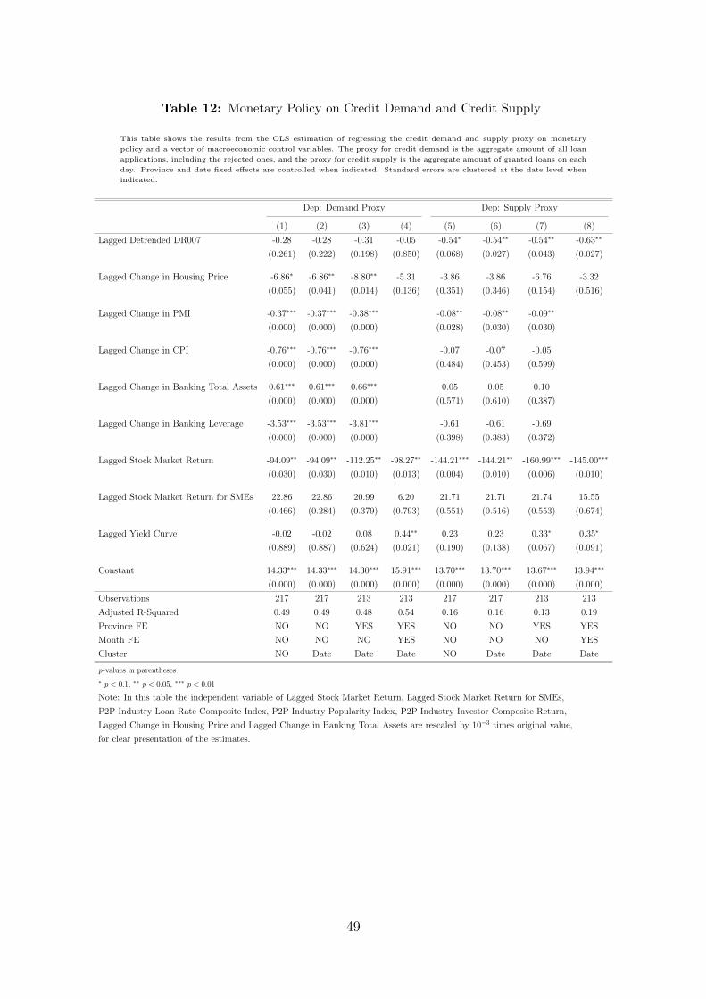
Table 12: Monetary Policy on Credit Demand and Credit Supply

This table shows the results from the OLS estimation of regressing the credit demand and supply proxy on monetary

policy and a vector of macroeconomic control variables. The proxy for credit demand is the aggregate amount of all loan

applications, including the rejected ones, and the proxy for credit supply is the aggregate amount of granted loans on each

day. Province and date fixed effects are controlled when indicated. Standard errors are clustered at the date level when

indicated.

Dep: Demand Proxy Dep: Supply Proxy

(1) (2) (3) (4) (5) (6) (7) (8)

Lagged Detrended DR007 -0.28 -0.28 -0.31 -0.05 -0.54∗ -0.54∗∗ -0.54∗∗ -0.63∗∗

(0.261) (0.222) (0.198) (0.850) (0.068) (0.027) (0.043) (0.027)

Lagged Change in Housing Price -6.86∗ -6.86∗∗ -8.80∗∗ -5.31 -3.86 -3.86 -6.76 -3.32

(0.055) (0.041) (0.014) (0.136) (0.351) (0.346) (0.154) (0.516)

Lagged Change in PMI -0.37∗∗∗ -0.37∗∗∗ -0.38∗∗∗ -0.08∗∗ -0.08∗∗ -0.09∗∗

(0.000) (0.000) (0.000) (0.028) (0.030) (0.030)

Lagged Change in CPI -0.76∗∗∗ -0.76∗∗∗ -0.76∗∗∗ -0.07 -0.07 -0.05

(0.000) (0.000) (0.000) (0.484) (0.453) (0.599)

Lagged Change in Banking Total Assets 0.61∗∗∗ 0.61∗∗∗ 0.66∗∗∗ 0.05 0.05 0.10

(0.000) (0.000) (0.000) (0.571) (0.610) (0.387)

Lagged Change in Banking Leverage -3.53∗∗∗ -3.53∗∗∗ -3.81∗∗∗ -0.61 -0.61 -0.69

(0.000) (0.000) (0.000) (0.398) (0.383) (0.372)

Lagged Stock Market Return -94.09∗∗ -94.09∗∗ -112.25∗∗ -98.27∗∗ -144.21∗∗∗ -144.21∗∗ -160.99∗∗∗ -145.00∗∗∗

(0.030) (0.030) (0.010) (0.013) (0.004) (0.010) (0.006) (0.010)

Lagged Stock Market Return for SMEs 22.86 22.86 20.99 6.20 21.71 21.71 21.74 15.55

(0.466) (0.284) (0.379) (0.793) (0.551) (0.516) (0.553) (0.674)

Lagged Yield Curve -0.02 -0.02 0.08 0.44∗∗ 0.23 0.23 0.33∗ 0.35∗

(0.889) (0.887) (0.624) (0.021) (0.190) (0.138) (0.067) (0.091)

Constant 14.33∗∗∗ 14.33∗∗∗ 14.30∗∗∗ 15.91∗∗∗ 13.70∗∗∗ 13.70∗∗∗ 13.67∗∗∗ 13.94∗∗∗

(0.000) (0.000) (0.000) (0.000) (0.000) (0.000) (0.000) (0.000)

Observations 217 217 213 213 217 217 213 213

Adjusted R-Squared 0.49 0.49 0.48 0.54 0.16 0.16 0.13 0.19

Province FE NO NO YES YES NO NO YES YES

Month FE NO NO NO YES NO NO NO YES

Cluster NO Date Date Date NO Date Date Date

p-values in parentheses

∗ p < 0.1, ∗∗ p < 0.05, ∗∗∗ p < 0.01

Note: In this table the independent variable of Lagged Stock Market Return, Lagged Stock Market Return for SMEs,

P2P Industry Loan Rate Composite Index, P2P Industry Popularity Index, P2P Industry Investor Composite Return,

Lagged Change in Housing Price and Lagged Change in Banking Total Assets are rescaled by 10−3 times original value,

for clear presentation of the estimates.

49

Table 13: OLS Analysis: Control Demand Proxy

This table shows the results from regressing the credit score of approved loan applications on monetary policy, the liquidity

of the platform, i.e. newly added loanable funding, the interaction between monetary policy and platform liquidity, and a

vector of control variables of the loan, borrower and macroeconomic conditions. Compared to the baseline estimates, we

add the proxy of credit demand in the control variables. In columns(1)-(2), we use the logarithm of aggregated amount of

all loan applications on each day as a proxy for credit demand, and in columns(3)-(4), we use the logarithm of number of

borrowers in the P2P market in each month as a proxy for credit demand. Province fixed effect is controlled, but month fixed

effect is not due to the monthly frequency of the second credit demand proxy. The estimates for borrower characteristics

are omitted here due to space limit. We use the sample of approved loan applications and employ OLS estimation for this

table. Standard errors are clustered at the borrower and date levels.

Total Loan Application Amount Aggregate Number of Borrowers

(1) (2) (3) (4)

Ln(Credit Score) Ln(Credit Score) Ln(Credit Score) Ln(Credit Score)

Lagged Detrended DR007 0.043∗∗∗ -0.051∗∗∗ 0.042∗∗∗ -0.044∗∗∗

(0.000) (0.000) (0.000) (0.002)

Log Lagged Liquidity 0.731∗∗ 0.402

(0.042) (0.265)

Lagged Detrended DR007 × Log Lagged Liquidity 20.948∗∗∗ 19.070∗∗∗

(0.000) (0.000)

Demand Proxy-Ln(Total Loan Application Amount) 0.002∗ 0.002∗

(0.081) (0.061)

Demand Proxy-Ln(Number of Borrowers in P2P Market) 0.023∗∗∗ 0.019∗∗∗

(0.000) (0.000)

Log Loan Amount 1.259∗∗∗ 1.202∗∗∗ 1.196∗∗∗ 1.153∗∗∗

(0.003) (0.006) (0.004) (0.009)

Loan Maturity -1.816∗∗∗ -1.814∗∗∗ -1.801∗∗∗ -1.802∗∗∗

(0.000) (0.000) (0.000) (0.000)

Loan Interest Rate -0.005∗∗∗ -0.005∗∗∗ -0.005∗∗∗ -0.005∗∗∗

(0.000) (0.000) (0.000) (0.000)

Lagged Stock Market Return 0.093 -0.412 -0.069 -0.646

(0.854) (0.434) (0.891) (0.217)

Lagged Stock Market Return for SMEs -0.273 -0.049 -0.162 0.047

(0.451) (0.897) (0.655) (0.901)

Lagged Yield Curve 0.022∗∗∗ 0.020∗∗∗ 0.020∗∗∗ 0.019∗∗∗

(0.000) (0.000) (0.000) (0.000)

P2P Industry Loan Rate Composite Index 0.622∗ 1.451∗∗∗ 0.292 1.127∗∗∗

(0.098) (0.001) (0.441) (0.008)

P2P Industry Popularity Index 0.069∗∗∗ 0.056∗∗∗ 0.072∗∗∗ 0.065∗∗∗

(0.000) (0.006) (0.000) (0.001)

P2P Industry Investor Composite Return 1.294 0.045 2.672 1.210

(0.445) (0.980) (0.114) (0.500)

Lagged Change in Housing Price -0.188∗∗ -0.145∗ -0.043 -0.036

(0.019) (0.076) (0.616) (0.679)

Lagged Change in Banking Total Assets 0.045∗∗∗ 0.046∗∗∗ 0.045∗∗∗ 0.047∗∗∗

(0.000) (0.000) (0.000) (0.000)

Lagged Change in Banking Leverage -0.246∗∗∗ -0.276∗∗∗ -0.254∗∗∗ -0.280∗∗∗

(0.000) (0.000) (0.000) (0.000)

Lagged Change in PMI -0.014∗∗∗ -0.014∗∗∗ -0.014∗∗∗ -0.015∗∗∗

(0.000) (0.000) (0.000) (0.000)

Lagged Change in CPI -0.022∗∗∗ -0.023∗∗∗ -0.024∗∗∗ -0.025∗∗∗

(0.000) (0.000) (0.000) (0.000)

Constant 6.415∗∗∗ 6.382∗∗∗ 6.244∗∗∗ 6.255∗∗∗

(0.000) (0.000) (0.000) (0.000)

Observations 10953 9922 10953 9922

Adjusted R-Squared 0.656 0.658 0.657 0.659

Loan Characteristics YES YES YES YES

Borrower Characteristics YES YES YES YES

Macro Characteristics YES YES YES YES

Borrower Province FE YES YES YES YES

Month FE NO NO NO NO

p-values in parentheses

In this table the independent variable of Log Lagged Liquidity, Log Loan Amount, Loan Maturity, Lagged Stock Market Return, Lagged Stock Market Return for SMES,

P2P Industry Loan Rate Composite Index, P2P Industry Popularity Index, P2P Industry Investor Composite Return,

Lagged Change in Housing Price and Lagged CHange in Banking Total Assets are rescaled by 10−3 times original value, for clear presentation of the estimates.

∗ p < 0.1, ∗∗ p < 0.05, ∗∗∗ p < 0.01 50

Table 14: Probit Analysis: Control Demand Proxy

This table shows the results from the Probit estimation of loan granting on monetary policy, the credit score of the loan

applicant, the liquidity of the platform, i.e. newly added loanable funding, the full interaction terms between these three

variables, and a vector of control variables of the loan, borrower and macroeconomic conditions. Compared to the baseline

estimates, we add the proxy of credit demand in the control variables. In columns(1)-(2), we use the logarithm of aggregated

amount of all loan applications on each day as a proxy for credit demand, and in columns(3)-(4), we use the logarithm

of number of borrowers in the P2P market in each month as a proxy for credit demand. The estimates for borrower

characteristics are omitted here due to space limit. Standard errors are clustered at the borrower and date levels.

Total Loan Application Amount Aggregate Number of Borrowers

(1) (2) (3) (4)

Granted Granted Granted Granted

Granted

Lagged Detrended DR007 -88.94∗∗ -70.51 -87.76∗∗ -75.66∗

(0.038) (0.106) (0.041) (0.084)

Ln(Credit Score) 7.88∗∗∗ 8.20∗∗∗ 7.81∗∗∗ 8.16∗∗∗

(0.000) (0.000) (0.000) (0.000)

Lagged Detrended DR007 × Ln(Credit Score) 13.64∗∗ 10.97 13.44∗∗ 11.74∗

(0.039) (0.104) (0.044) (0.083)

Lagged Liquidity 4.25∗∗∗ 2.90∗∗∗ 4.35∗∗∗ 2.94∗∗∗

(0.000) (0.001) (0.000) (0.001)

Ln(Credit Score) × Lagged Liquidity -0.65∗∗∗ -0.45∗∗∗ -0.66∗∗∗ -0.46∗∗∗

(0.000) (0.001) (0.000) (0.001)

Lagged Detrended DR007 × Lagged Liquidity 13.06 12.99 12.87 14.36

(0.169) (0.178) (0.178) (0.138)

Lagged Detrended DR007 × Ln(Credit Score) × Lagged Liquidity -2.00 -2.03 -1.97 -2.24

(0.172) (0.173) (0.183) (0.134)

Demand Proxy-Ln(Total Loan Application Amount) -0.10∗∗∗ -0.13∗∗∗

(0.000) (0.000)

Demand Proxy-Ln(Number of Borrowers in P2P Market) -0.13∗ -0.21∗∗

(0.090) (0.024)

Log Loan Amount -0.25∗∗∗ -0.26∗∗∗ -0.25∗∗∗ -0.26∗∗∗

(0.000) (0.000) (0.000) (0.000)

Loan Maturity -0.02∗∗∗ -0.02∗∗∗ -0.03∗∗∗ -0.02∗∗∗

(0.000) (0.000) (0.000) (0.000)

Loan Interest Rate -0.01∗∗∗ -0.00∗∗∗ -0.01∗∗∗ -0.01∗∗∗

(0.000) (0.004) (0.000) (0.002)

Constant -47.73∗∗∗ -47.49∗∗∗ -47.85∗∗∗ -47.61∗∗∗

(0.000) (0.000) (0.000) (0.000)

Observations 66236 54113 66236 54113

Loan Characteristics YES YES YES YES

Borrower Characteristics YES YES YES YES

Borrower FE NO NO NO NO

Time FE NO NO NO NO

p-values in parentheses

∗ p < 0.1, ∗∗ p < 0.05, ∗∗∗ p < 0.01

51

Table 15: Riskiness of Credit Allocation and Monetary Policy

This table shows the results from regressing the platform-level riskiness of credit allocation on monetary policy and a

vector of control variables of the macroeconomic conditions. We use the detrended DR007 to proxy monetary policy in

columns(1)-(4), and the dummy of easing and normal periods to capture the effect of monetary policy in columns(5)-(8).

Easing periods are defined to days when the monetary policy rate is below its 25th percentile and normal periods are defined

as days when the rates lie within the [25th, 75th] percentile. We employ OLS estimation and robust standard errors for

this table.

(1) (2) (3) (4) (5) (6) (7) (8)

Detrended DR007 -1.55∗ -1.47∗ -1.66∗ -1.58

(0.074) (0.087) (0.097) (0.109)

Easing Periods 0.43∗∗ 0.43∗∗ 0.48∗∗ 0.47∗∗

(0.043) (0.044) (0.039) (0.039)

Normal Periods 0.39∗∗ 0.39∗∗ 0.47∗∗ 0.46∗∗

(0.036) (0.039) (0.014) (0.015)

Proxy of Aggregate Demand 0.09 0.08 0.13 0.12

(0.609) (0.688) (0.460) (0.540)

Lagged Stock Market Return 0.18 0.18 0.18 0.19

(0.251) (0.236) (0.229) (0.208)

Lagged Stock Market Return for SMEs -0.02 -0.02 -0.04 -0.04

(0.897) (0.877) (0.762) (0.755)

Lagged Yield Curve 0.43 0.40 0.48 0.42

(0.304) (0.351) (0.218) (0.292)

P2P Industry Loan Rate Composite Index 0.03 0.03 0.01 0.01

(0.723) (0.753) (0.904) (0.930)

P2P Industry Popularity Index -0.01 -0.01 -0.01 -0.01

(0.173) (0.172) (0.124) (0.128)

P2P Industry Investor Composite Return 0.06 0.05 0.15 0.14

(0.875) (0.888) (0.692) (0.701)

Constant -1.06∗∗∗ -2.51 -2.05 -3.13 -1.37∗∗∗ -3.44 -2.31 -4.10

(0.000) (0.379) (0.482) (0.436) (0.000) (0.226) (0.432) (0.303)

Observations 233 233 219 219 233 233 219 219

p-values in parentheses

∗ p < 0.1, ∗∗ p < 0.05, ∗∗∗ p < 0.01

52

Table 16: Robustness Check: Granted Loan Analysis Using Monthly Monetary Policy Rates

This table shows the results from regressing the credit score of approved loan applications on monetary policy, the liquidity

of the platform, i.e. newly added loanable funding, the interaction between monetary policy and platform liquidity, and a

vector of control variables of the loan, borrower and macroeconomic conditions. Compared to the baseline estimates, we

use the monthly monetary policy variables here. Province fixed effect is controlled, but month fixed effect is not due to the

now monthly frequency of the monetary policy. The estimates for borrower characteristics are omitted here due to space

limit. We use the sample of approved loan applications and employ OLS estimation for this table. Standard errors are

clustered at the borrower and month levels.

(1) (2) (3) (4) (5) (6)

Ln(Credit Score) Ln(Credit Score) Ln(Credit Score) Ln(Credit Score) Ln(Credit Score) Ln(Credit Score)

Lagged Detrended DR007(Monthly) 0.22∗∗∗ 0.21∗∗∗ 0.13∗∗∗ 0.43∗∗∗ -4.43∗∗∗

(0.000) (0.000) (0.000) (0.000) (0.000)

Log Lagged Liquidity(Monthly) -0.01∗∗∗ -0.02∗∗∗ -0.01∗∗∗

(0.000) (0.000) (0.000)

Lagged Detrended DR007(Monthly) × Log Lagged Liquidity(Monthly) 0.56∗∗∗

(0.000)

Log Loan Amount 0.50 0.79∗ 0.93∗∗ 0.86∗ 0.86∗

(0.270) (0.092) (0.048) (0.062) (0.062)

Loan Maturity -1.64∗∗∗ -1.76∗∗∗ -1.80∗∗∗ -1.78∗∗∗ -1.78∗∗∗

(0.000) (0.000) (0.000) (0.000) (0.000)

Loan Interest Rate -0.01∗∗∗ -0.01∗∗∗ -0.01∗∗∗ -0.01∗∗∗ -0.01∗∗∗

(0.000) (0.000) (0.000) (0.000) (0.000)

Lagged Stock Market Return -0.06 0.12 -0.54 -0.54

(0.901) (0.819) (0.284) (0.284)

Lagged Stock Market Return for SMEs 0.90∗∗ 0.69∗ 0.68∗ 0.68∗

(0.010) (0.051) (0.052) (0.052)

Lagged Yield Curve -0.01∗∗∗ -0.01∗∗∗ 0.00 0.00

(0.000) (0.004) (0.166) (0.166)

P2P Industry Loan Rate Composite Index 1.88∗∗∗ 2.80∗∗∗ 1.15∗∗∗ 1.15∗∗∗

(0.000) (0.000) (0.003) (0.003)

P2P Industry Popularity Index 0.07∗∗∗ 0.08∗∗∗ 0.05∗∗∗ 0.05∗∗∗

(0.000) (0.000) (0.010) (0.010)

P2P Industry Investor Composite Return -2.43 -6.99∗∗∗ -1.52 -1.52

(0.166) (0.000) (0.382) (0.382)

Lagged Change in Housing Price -0.11 -0.43∗∗∗ -0.12 -0.12

(0.219) (0.000) (0.186) (0.186)

Lagged Change in Banking Total Assets 0.00 -0.01∗∗∗ -0.02∗∗∗ -0.00

(0.433) (0.000) (0.000) (0.429)

Lagged Change in Banking Leverage -0.04∗∗∗ 0.02 0.10∗∗∗ -0.01

(0.001) (0.250) (0.000) (0.619)

Lagged Change in PMI -0.00∗∗∗ -0.00 0.01∗∗∗ 0.00∗∗∗

(0.000) (0.102) (0.000) (0.000)

Lagged Change in CPI -0.02∗∗∗ -0.02∗∗∗ 0.02∗∗∗ 0.00

(0.000) (0.000) (0.000) (.)

Constant 6.47∗∗∗ 6.56∗∗∗ 6.50∗∗∗ 6.59∗∗∗ 6.76∗∗∗ 6.61∗∗∗

(0.000) (0.000) (0.000) (0.000) (0.000) (0.000)

Observations 10361 10361 9358 9358 9358 9358

Adjusted R-Squared 0.03 0.64 0.66 0.66 0.67 0.67

Loan Characteristics NO YES YES YES YES YES

Borrower Characteristics NO YES YES YES YES YES

Macro Characteristics NO NO YES YES YES YES

Borrower Province FE YES YES YES YES YES YES

Month FE NO NO NO NO NO NO

p-values in parentheses

In this table the independent variable of Log Lagged Liquidity, Log Loan Amount, Loan Maturity, Lagged Stock Market Return, Lagged Stock Market Return for SMES,

P2P Industry Loan Rate Composite Index, P2P Industry Popularity Index, P2P Industry Investor Composite Return, Lagged Change in Housing Price and Lagged Change

in Banking Total Assets are rescaled by 10−3 times original value, for clear presentation of the estimates.

∗ p < 0.1, ∗∗ p < 0.05, ∗∗∗ p < 0.01

53

Table 17: Robustness Check: Probit Analysis Using Monthly Monetary Policy Rates

This table shows the results from the Probit estimation of loan granting on monetary policy, the credit score of the loan

applicant, the liquidity of the platform, i.e. newly added loanable funding, the full interaction terms between these three

variables, and a vector of control variables of the loan, borrower and macroeconomic conditions. Compared to the baseline

estimates, we use the monthly monetary policy variables here. The estimates for borrower characteristics are omitted here

due to space limit. Standard errors are clustered at the borrower and month levels.

(1) (2) (3) (4) (5) (6) (7)

Granted Granted Granted Granted Granted Granted Granted

Granted

Lagged Detrended DR007(Monthly) -0.72∗∗∗ -244.90∗∗∗ -1695.44 -935.48 -1763.25 -150.63∗∗∗

(0.007) (0.000) (0.197) (0.477) (0.192) (0.004)

Ln(Credit Score) 5.73∗∗∗ 15.33∗∗∗ 18.44∗∗∗ 17.43∗∗∗ 19.58∗∗∗ 20.94∗∗∗

(0.000) (0.000) (0.000) (0.000) (0.000) (0.000)

Lagged Detrended DR007(Monthly) × Ln(Credit Score) 37.74∗∗∗ 250.76 130.26 258.37 251.46

(0.000) (0.218) (0.522) (0.216) (0.317)

Log Lagged Liquidity(Monthly) 7.77∗∗∗ 10.24∗∗∗ 8.96∗∗∗ 10.80∗∗∗ 7.06∗∗

(0.000) (0.003) (0.010) (0.002) (0.022)

Log Lagged Liquidity(Monthly) × Ln(Credit Score) -1.18∗∗∗ -1.52∗∗∗ -1.32∗∗ -1.61∗∗∗ -1.80∗∗∗

(0.000) (0.004) (0.014) (0.003) (0.002)

Lagged Detrended DR007(Monthly) × Log Lagged Liquidity(Monthly) 179.83 85.98 183.34 0.00

(0.243) (0.577) (0.247) (.)

Lagged Detrended DR007(Monthly) × Ln(Credit Score) × Log Lagged Liquidity(Monthly) -26.52 -11.66 -26.72 -26.23

(0.266) (0.625) (0.275) (0.372)

Log Loan Amount -198.62∗∗∗ -254.50∗∗∗ -258.77∗∗∗

(0.000) (0.000) (0.000)

Loan Maturity -23.11∗∗∗ -23.24∗∗∗ -25.59∗∗∗

(0.000) (0.000) (0.000)

Loan Interest Rate 0.00 -0.00 -0.00∗∗

(0.984) (0.369) (0.028)

Lagged Change in Housing Price 2.94

(0.100)

Lagged Change in Banking Total Assets -5.40

(0.308)

Lagged Change in Banking Leverage 35.23

(0.321)

Lagged Stock Market Return -25.50∗∗

(0.022)

Lagged Stock Market Return for SMEs 3.98

(0.601)

Lagged Yield Curve -0.05

(0.357)

P2P Industry Loan Rate Composite Index -7.23

(0.414)

P2P Industry Popularity Index 0.96∗∗

(0.027)

P2P Industry Investor Composite Return -30.13

(0.467)

Lagged Change in PMI 1.91

(0.328)

Lagged Change in CPI 5.23

(0.355)

Constant -0.92∗∗∗ -37.91∗∗∗ -101.30∗∗∗ -123.16∗∗∗ -114.60∗∗∗ -127.95∗∗∗ -85.25∗∗

(0.000) (0.000) (0.000) (0.000) (0.000) (0.000) (0.011)

Observations 64353 64353 64353 64353 64353 64353 52335

Loan Characteristics NO NO NO NO YES YES YES

Borrower Characteristics NO NO NO NO NO YES YES

Macro Characteristics NO NO NO NO NO NO YES

Borrower FE NO NO NO NO NO NO NO

Time FE NO NO NO NO NO NO NO

p-values in parentheses

∗ p < 0.1, ∗∗ p < 0.05, ∗∗∗ p < 0.01 54

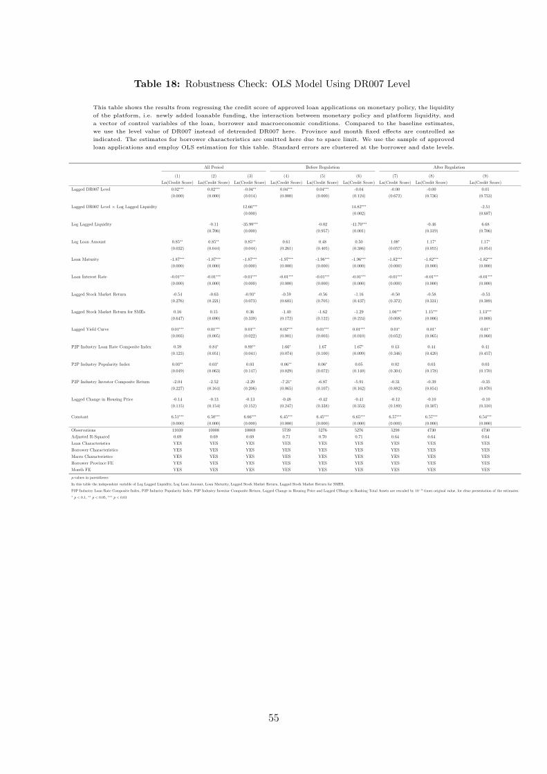
Table 18: Robustness Check: OLS Model Using DR007 Level

This table shows the results from regressing the credit score of approved loan applications on monetary policy, the liquidity

of the platform, i.e. newly added loanable funding, the interaction between monetary policy and platform liquidity, and

a vector of control variables of the loan, borrower and macroeconomic conditions. Compared to the baseline estimates,

we use the level value of DR007 instead of detrended DR007 here. Province and month fixed effects are controlled as

indicated. The estimates for borrower characteristics are omitted here due to space limit. We use the sample of approved

loan applications and employ OLS estimation for this table. Standard errors are clustered at the borrower and date levels.

All Period Before Regulation After Regulation

(1) (2) (3) (4) (5) (6) (7) (8) (9)

Ln(Credit Score) Ln(Credit Score) Ln(Credit Score) Ln(Credit Score) Ln(Credit Score) Ln(Credit Score) Ln(Credit Score) Ln(Credit Score) Ln(Credit Score)

Lagged DR007 Level 0.02∗∗∗ 0.02∗∗∗ -0.04∗∗ 0.04∗∗∗ 0.04∗∗∗ -0.04 -0.00 -0.00 0.01

(0.000) (0.000) (0.014) (0.000) (0.000) (0.124) (0.672) (0.736) (0.753)

Lagged DR007 Level × Log Lagged Liquidity 12.66∗∗∗ 14.82∗∗∗ -2.51

(0.000) (0.002) (0.687)

Log Lagged Liquidity -0.11 -35.99∗∗∗ -0.02 -41.70∗∗∗ -0.46 6.68

(0.706) (0.000) (0.957) (0.001) (0.319) (0.706)

Log Loan Amount 0.85∗∗ 0.85∗∗ 0.85∗∗ 0.61 0.48 0.50 1.08∗ 1.17∗ 1.17∗

(0.032) (0.044) (0.044) (0.261) (0.405) (0.386) (0.057) (0.055) (0.054)

Loan Maturity -1.87∗∗∗ -1.87∗∗∗ -1.87∗∗∗ -1.97∗∗∗ -1.96∗∗∗ -1.96∗∗∗ -1.82∗∗∗ -1.82∗∗∗ -1.82∗∗∗

(0.000) (0.000) (0.000) (0.000) (0.000) (0.000) (0.000) (0.000) (0.000)

Loan Interest Rate -0.01∗∗∗ -0.01∗∗∗ -0.01∗∗∗ -0.01∗∗∗ -0.01∗∗∗ -0.01∗∗∗ -0.01∗∗∗ -0.01∗∗∗ -0.01∗∗∗

(0.000) (0.000) (0.000) (0.000) (0.000) (0.000) (0.000) (0.000) (0.000)

Lagged Stock Market Return -0.54 -0.63 -0.93∗ -0.59 -0.56 -1.16 -0.50 -0.58 -0.53

(0.276) (0.221) (0.073) (0.681) (0.705) (0.437) (0.372) (0.331) (0.389)

Lagged Stock Market Return for SMEs 0.16 0.15 0.36 -1.40 -1.62 -1.29 1.06∗∗∗ 1.15∗∗∗ 1.13∗∗∗

(0.647) (0.690) (0.339) (0.172) (0.122) (0.224) (0.008) (0.006) (0.008)

Lagged Yield Curve 0.01∗∗∗ 0.01∗∗∗ 0.01∗∗ 0.02∗∗∗ 0.01∗∗∗ 0.01∗∗∗ 0.01∗ 0.01∗ 0.01∗

(0.003) (0.005) (0.022) (0.001) (0.003) (0.010) (0.052) (0.065) (0.060)

P2P Industry Loan Rate Composite Index 0.59 0.84∗ 0.88∗∗ 1.66∗ 1.67 1.67∗ 0.43 0.44 0.41

(0.123) (0.051) (0.041) (0.074) (0.100) (0.099) (0.346) (0.420) (0.457)

P2P Industry Popularity Index 0.03∗∗ 0.03∗ 0.03 0.06∗∗ 0.06∗ 0.05 0.02 0.03 0.03

(0.049) (0.063) (0.147) (0.029) (0.072) (0.140) (0.304) (0.178) (0.170)

P2P Industry Investor Composite Return -2.04 -2.52 -2.29 -7.21∗ -6.87 -5.91 -0.31 -0.39 -0.35

(0.227) (0.164) (0.206) (0.065) (0.107) (0.162) (0.882) (0.854) (0.870)

Lagged Change in Housing Price -0.14 -0.13 -0.13 -0.48 -0.42 -0.41 -0.12 -0.10 -0.10

(0.115) (0.154) (0.152) (0.247) (0.338) (0.353) (0.189) (0.307) (0.310)

Constant 6.51∗∗∗ 6.50∗∗∗ 6.66∗∗∗ 6.45∗∗∗ 6.45∗∗∗ 6.65∗∗∗ 6.57∗∗∗ 6.57∗∗∗ 6.54∗∗∗

(0.000) (0.000) (0.000) (0.000) (0.000) (0.000) (0.000) (0.000) (0.000)

Observations 11039 10008 10008 5739 5276 5276 5298 4730 4730

Adjusted R-Squared 0.69 0.69 0.69 0.71 0.70 0.71 0.64 0.64 0.64

Loan Characteristics YES YES YES YES YES YES YES YES YES

Borrower Characteristics YES YES YES YES YES YES YES YES YES

Macro Characteristics YES YES YES YES YES YES YES YES YES

Borrower Province FE YES YES YES YES YES YES YES YES YES

Month FE YES YES YES YES YES YES YES YES YES

p-values in parentheses

In this table the independent variable of Log Lagged Liquidity, Log Loan Amount, Loan Maturity, Lagged Stock Market Return, Lagged Stock Market Return for SMES,

P2P Industry Loan Rate Composite Index, P2P Industry Popularity Index, P2P Industry Investor Composite Return, Lagged Change in Housing Price and Lagged CHange in Banking Total Assets are rescaled by 10−3 times original value, for clear presentation of the estimates.

∗ p < 0.1, ∗∗ p < 0.05, ∗∗∗ p < 0.01

55

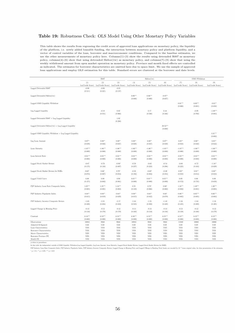
Table 19: Robustness Check: OLS Model Using Other Monetary Policy Variables

This table shows the results from regressing the credit score of approved loan applications on monetary policy, the liquidity

of the platform, i.e. newly added loanable funding, the interaction between monetary policy and platform liquidity, and a

vector of control variables of the loan, borrower and macroeconomic conditions. Compared to the baseline estimates, we

use the other measurements of monetary policy here. Columns(1)-(3) show the results using detrended R007 as monetary

policy, columns(4)-(6) show that using detrended Shibor(1w) as monetary policy, and columns(7)-(9) show that using the

weekly withdrawal amount from open market operation as monetary policy. Province and month fixed effects are controlled

as indicated. The estimates for borrower characteristics are omitted here due to space limit. We use the sample of approved

loan applications and employ OLS estimation for this table. Standard errors are clustered at the borrower and date levels.

R007 Shibor(1w) OMO Withdraw

(1) (2) (3) (4) (5) (6) (7) (8) (9)

Ln(Credit Score) Ln(Credit Score) Ln(Credit Score) Ln(Credit Score) Ln(Credit Score) Ln(Credit Score) Ln(Credit Score) Ln(Credit Score) Ln(Credit Score)

Lagged Detrended R007 -0.00 -0.00 -0.01

(0.511) (0.321) (0.137)

Lagged Detrended Shibor(1w) 0.06∗∗∗ 0.06∗∗∗ -0.07∗∗

(0.000) (0.000) (0.037)

Lagged OMO Liquidity Withdraw 0.01∗∗∗ 0.00∗∗∗ -0.01∗∗

(0.000) (0.001) (0.050)

Log Lagged Liquidity -0.18 0.02 0.17 0.44 -0.09 -1.88∗∗∗

(0.551) (0.960) (0.580) (0.166) (0.760) (0.004)

Lagged Detrended R007 × Log Lagged Liquidity 1.02

(0.206)

Lagged Detrended Shibor(1w) × Log Lagged Liquidity 28.53∗∗∗

(0.000)

Lagged OMO Liquidity Withdraw × Log Lagged Liquidity 3.31∗∗∗

(0.002)

Log Loan Amount 0.87∗∗ 0.88∗∗ 0.88∗∗ 0.88∗∗ 0.88∗∗ 0.87∗∗ 0.85∗∗ 0.86∗∗ 0.85∗∗

(0.029) (0.036) (0.037) (0.028) (0.037) (0.039) (0.032) (0.040) (0.043)

Loan Maturity -1.87∗∗∗ -1.86∗∗∗ -1.86∗∗∗ -1.86∗∗∗ -1.86∗∗∗ -1.85∗∗∗ -1.87∗∗∗ -1.86∗∗∗ -1.86∗∗∗

(0.000) (0.000) (0.000) (0.000) (0.000) (0.000) (0.000) (0.000) (0.000)

Loan Interest Rate -0.01∗∗∗ -0.01∗∗∗ -0.01∗∗∗ -0.01∗∗∗ -0.01∗∗∗ -0.01∗∗∗ -0.01∗∗∗ -0.01∗∗∗ -0.01∗∗∗

(0.000) (0.000) (0.000) (0.000) (0.000) (0.000) (0.000) (0.000) (0.000)

Lagged Stock Market Return -0.67 -0.76 -0.90∗ -0.59 -0.63 -0.54 -0.60 -0.72 -1.16∗∗

(0.175) (0.140) (0.087) (0.237) (0.223) (0.296) (0.225) (0.163) (0.029)

Lagged Stock Market Return for SMEs 0.63∗ 0.66∗ 0.70∗ -0.50 -0.69∗ -0.38 0.93∗∗ 0.91∗∗ 0.88∗∗

(0.072) (0.067) (0.053) (0.192) (0.084) (0.353) (0.010) (0.014) (0.018)

Lagged Yield Curve 0.00 0.00 0.00 0.01∗∗∗ 0.01∗∗∗ 0.01∗∗∗ 0.00 0.00 0.00

(0.475) (0.802) (0.981) (0.000) (0.000) (0.000) (0.572) (0.735) (0.659)

P2P Industry Loan Rate Composite Index 1.05∗∗∗ 1.35∗∗∗ 1.34∗∗∗ 0.55 0.78∗ 0.80∗ 1.16∗∗∗ 1.40∗∗∗ 1.26∗∗∗

(0.005) (0.001) (0.002) (0.149) (0.066) (0.060) (0.002) (0.001) (0.003)

P2P Industry Popularity Index 0.04∗∗ 0.04∗∗ 0.04∗∗ 0.04∗∗ 0.04∗∗ 0.03∗ 0.06∗∗∗ 0.05∗∗∗ 0.06∗∗∗

(0.015) (0.019) (0.029) (0.015) (0.032) (0.079) (0.002) (0.005) (0.004)

P2P Industry Investor Composite Return -1.65 -2.31 -2.17 -1.04 -1.55 -1.43 -1.34 -1.84 -1.24

(0.329) (0.204) (0.233) (0.535) (0.392) (0.429) (0.425) (0.309) (0.495)

Lagged Change in Housing Price -0.13 -0.12 -0.12 -0.14 -0.13 -0.13 -0.13 -0.12 -0.12

(0.134) (0.178) (0.178) (0.102) (0.134) (0.134) (0.128) (0.168) (0.179)

Constant 6.54∗∗∗ 6.53∗∗∗ 6.53∗∗∗ 6.56∗∗∗ 6.55∗∗∗ 6.55∗∗∗ 6.53∗∗∗ 6.52∗∗∗ 6.53∗∗∗

(0.000) (0.000) (0.000) (0.000) (0.000) (0.000) (0.000) (0.000) (0.000)

Observations 10953 9922 9922 10953 9922 9922 11039 10008 10008

Adjusted R-Squared 0.68 0.68 0.68 0.69 0.68 0.69 0.69 0.69 0.69

Loan Characteristics YES YES YES YES YES YES YES YES YES

Borrower Characteristics YES YES YES YES YES YES YES YES YES

Macro Characteristics YES YES YES YES YES YES YES YES YES

Borrower Province FE YES YES YES YES YES YES YES YES YES

Month FE YES YES YES YES YES YES YES YES YES

p-values in parentheses

In this table the independent variable of OMO Liquidity Withdraw,Log Lagged Liquidity, Log Loan Amount, Loan Maturity, Lagged Stock Market Return, Lagged Stock Market Return for SMES,

P2P Industry Loan Rate Composite Index, P2P Industry Popularity Index, P2P Industry Investor Composite Return, Lagged Change in Housing Price and Lagged CHange in Banking Total Assets are rescaled by 10−3 times original value, for clear presentation of the estimates.

∗ p < 0.1, ∗∗ p < 0.05, ∗∗∗ p < 0.01

56

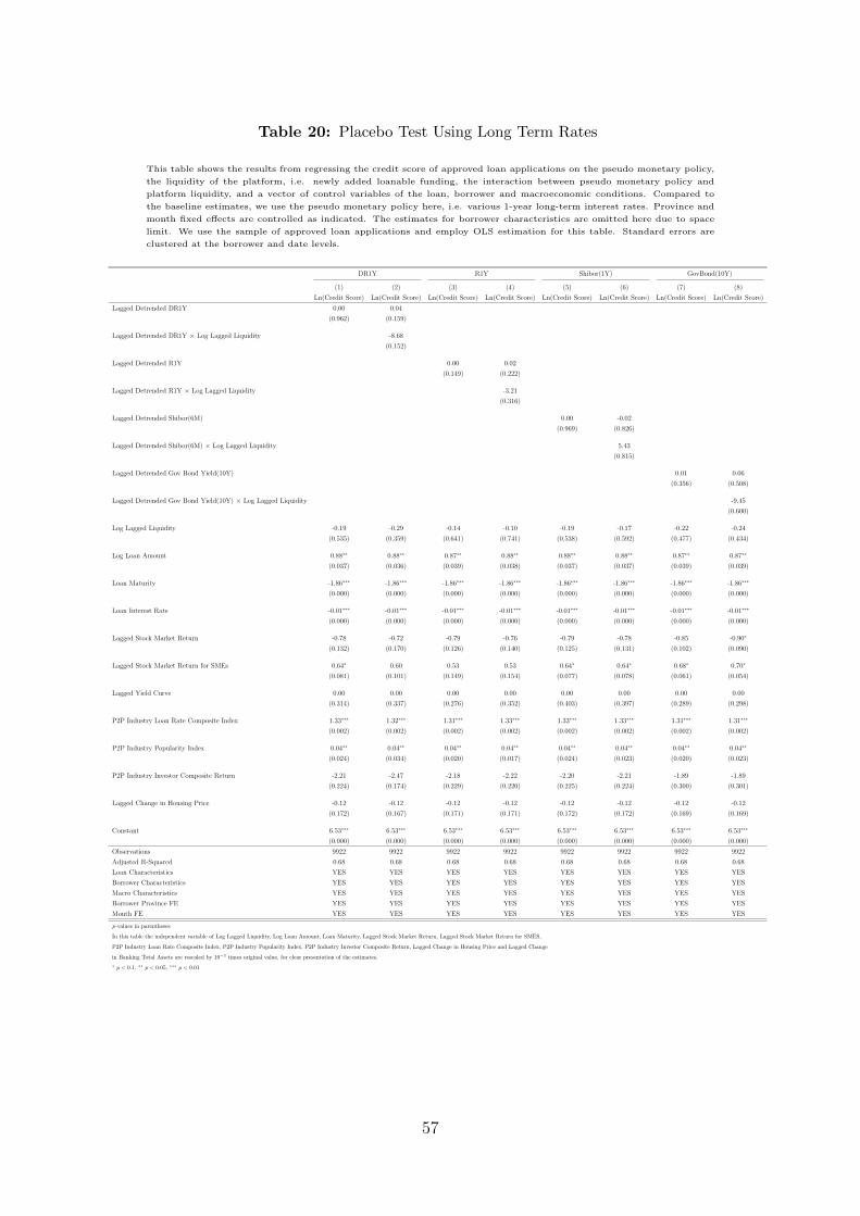
Table 20: Placebo Test Using Long Term Rates

This table shows the results from regressing the credit score of approved loan applications on the pseudo monetary policy,

the liquidity of the platform, i.e. newly added loanable funding, the interaction between pseudo monetary policy and

platform liquidity, and a vector of control variables of the loan, borrower and macroeconomic conditions. Compared to

the baseline estimates, we use the pseudo monetary policy here, i.e. various 1-year long-term interest rates. Province and

month fixed effects are controlled as indicated. The estimates for borrower characteristics are omitted here due to space

limit. We use the sample of approved loan applications and employ OLS estimation for this table. Standard errors are

clustered at the borrower and date levels.

DR1Y R1Y Shibor(1Y) GovBond(10Y)

(1) (2) (3) (4) (5) (6) (7) (8)

Ln(Credit Score) Ln(Credit Score) Ln(Credit Score) Ln(Credit Score) Ln(Credit Score) Ln(Credit Score) Ln(Credit Score) Ln(Credit Score)

Lagged Detrended DR1Y 0.00 0.04

(0.962) (0.159)

Lagged Detrended DR1Y × Log Lagged Liquidity -8.68

(0.152)

Lagged Detrended R1Y 0.00 0.02

(0.149) (0.222)

Lagged Detrended R1Y × Log Lagged Liquidity -3.21

(0.316)

Lagged Detrended Shibor(6M) 0.00 -0.02

(0.969) (0.826)

Lagged Detrended Shibor(6M) × Log Lagged Liquidity 5.43

(0.815)

Lagged Detrended Gov Bond Yield(10Y) 0.01 0.06

(0.356) (0.508)

Lagged Detrended Gov Bond Yield(10Y) × Log Lagged Liquidity -9.45

(0.600)

Log Lagged Liquidity -0.19 -0.29 -0.14 -0.10 -0.19 -0.17 -0.22 -0.24

(0.535) (0.359) (0.641) (0.741) (0.538) (0.592) (0.477) (0.434)

Log Loan Amount 0.88∗∗ 0.88∗∗ 0.87∗∗ 0.88∗∗ 0.88∗∗ 0.88∗∗ 0.87∗∗ 0.87∗∗

(0.037) (0.036) (0.039) (0.038) (0.037) (0.037) (0.039) (0.039)

Loan Maturity -1.86∗∗∗ -1.86∗∗∗ -1.86∗∗∗ -1.86∗∗∗ -1.86∗∗∗ -1.86∗∗∗ -1.86∗∗∗ -1.86∗∗∗

(0.000) (0.000) (0.000) (0.000) (0.000) (0.000) (0.000) (0.000)

Loan Interest Rate -0.01∗∗∗ -0.01∗∗∗ -0.01∗∗∗ -0.01∗∗∗ -0.01∗∗∗ -0.01∗∗∗ -0.01∗∗∗ -0.01∗∗∗

(0.000) (0.000) (0.000) (0.000) (0.000) (0.000) (0.000) (0.000)

Lagged Stock Market Return -0.78 -0.72 -0.79 -0.76 -0.79 -0.78 -0.85 -0.90∗

(0.132) (0.170) (0.126) (0.140) (0.125) (0.131) (0.102) (0.090)

Lagged Stock Market Return for SMEs 0.64∗ 0.60 0.53 0.53 0.64∗ 0.64∗ 0.68∗ 0.70∗

(0.081) (0.101) (0.149) (0.154) (0.077) (0.078) (0.061) (0.054)

Lagged Yield Curve 0.00 0.00 0.00 0.00 0.00 0.00 0.00 0.00

(0.314) (0.337) (0.276) (0.352) (0.403) (0.397) (0.289) (0.298)

P2P Industry Loan Rate Composite Index 1.33∗∗∗ 1.32∗∗∗ 1.31∗∗∗ 1.33∗∗∗ 1.33∗∗∗ 1.33∗∗∗ 1.31∗∗∗ 1.31∗∗∗

(0.002) (0.002) (0.002) (0.002) (0.002) (0.002) (0.002) (0.002)

P2P Industry Popularity Index 0.04∗∗ 0.04∗∗ 0.04∗∗ 0.04∗∗ 0.04∗∗ 0.04∗∗ 0.04∗∗ 0.04∗∗

(0.024) (0.034) (0.020) (0.017) (0.024) (0.023) (0.020) (0.023)

P2P Industry Investor Composite Return -2.21 -2.47 -2.18 -2.22 -2.20 -2.21 -1.89 -1.89

(0.224) (0.174) (0.229) (0.220) (0.225) (0.224) (0.300) (0.301)

Lagged Change in Housing Price -0.12 -0.12 -0.12 -0.12 -0.12 -0.12 -0.12 -0.12

(0.172) (0.167) (0.171) (0.171) (0.172) (0.172) (0.169) (0.169)

Constant 6.53∗∗∗ 6.53∗∗∗ 6.53∗∗∗ 6.53∗∗∗ 6.53∗∗∗ 6.53∗∗∗ 6.53∗∗∗ 6.53∗∗∗

(0.000) (0.000) (0.000) (0.000) (0.000) (0.000) (0.000) (0.000)

Observations 9922 9922 9922 9922 9922 9922 9922 9922

Adjusted R-Squared 0.68 0.68 0.68 0.68 0.68 0.68 0.68 0.68

Loan Characteristics YES YES YES YES YES YES YES YES

Borrower Characteristics YES YES YES YES YES YES YES YES

Macro Characteristics YES YES YES YES YES YES YES YES

Borrower Province FE YES YES YES YES YES YES YES YES

Month FE YES YES YES YES YES YES YES YES

p-values in parentheses

In this table the independent variable of Log Lagged Liquidity, Log Loan Amount, Loan Maturity, Lagged Stock Market Return, Lagged Stock Market Return for SMES,

P2P Industry Loan Rate Composite Index, P2P Industry Popularity Index, P2P Industry Investor Composite Return, Lagged Change in Housing Price and Lagged Change

in Banking Total Assets are rescaled by 10−3 times original value, for clear presentation of the estimates.

∗ p < 0.1, ∗∗ p < 0.05, ∗∗∗ p < 0.01

57

Table 21: Placebo Test Probit Model Using Long Term Rates

This table shows the results from the Probit estimation of loan granting on pseudo monetary policy, the credit score of the

loan applicant, the liquidity of the platform, i.e. newly added loanable funding, the full interaction terms between these

three variables, and a vector of control variables of the loan, borrower and macroeconomic conditions. Compared to the

baseline estimates, we use the pseudo monetary policy here, i.e. various 1-year long-term interest rates. The estimates for

borrower characteristics are omitted here due to space limit. Standard errors are clustered at the borrower and date levels.

DR1Y R1Y Shibor(1Y) GovBond(10Y)

(1) (2) (3) (4) (5) (6) (7) (8)

Granted Granted Granted Granted Granted Granted Granted Granted

Granted

Lagged Detrended DR1Y 63.92∗∗∗ -92.42

(0.003) (0.305)

Lagged Detrended DR1Y × Ln(Credit Score) -9.82∗∗∗ 13.71

(0.004) (0.325)

Lagged Detrended R1Y -11.08 19.59

(0.108) (0.616)

Lagged Detrended R1Y × Ln(Credit Score) 1.71 -3.10

(0.110) (0.608)

Lagged Detrended Shibor(1Y) 39.75 -104.10

(0.695) (0.875)

Lagged Detrended Shibor(1Y) × Ln(Credit Score) -6.19 15.85

(0.693) (0.877)

Lagged Detrended Gov Bond Yield(10Y) 20.80 -306.59

(0.622) (0.259)

Lagged Detrended Gov Bond Yield(10Y) × Ln(Credit Score) -3.23 47.38

(0.621) (0.260)

Log Lagged Liquidity 3098.23∗∗∗ 3031.26∗∗∗ 2786.30∗∗∗ 2856.23∗∗∗

(0.000) (0.000) (0.001) (0.001)

Lagged Detrended DR1Y × Log Lagged Liquidity 22382.22

(0.232)

Ln(Credit Score) × Log Lagged Liquidity -478.39∗∗∗ -470.13∗∗∗ -431.75∗∗∗ -442.61∗∗∗

(0.000) (0.000) (0.001) (0.001)

Lagged Detrended DR1Y × Ln(Credit Score) × Log Lagged Liquidity -3314.94

(0.252)

Lagged Detrended R1Y × Log Lagged Liquidity -8708.64

(0.381)

Lagged Detrended R1Y × Ln(Credit Score) × Log Lagged Liquidity 1362.24

(0.376)

Lagged Detrended Shibor(1Y) × Log Lagged Liquidity 34707.04

(0.818)

Lagged Detrended Shibor(1Y) × Ln(Credit Score) × Log Lagged Liquidity -5327.50

(0.819)

Lagged Detrended Gov Bond Yield(10Y) × Log Lagged Liquidity 66661.22

(0.233)

Lagged Detrended Gov Bond Yield(10Y) × Ln(Credit Score) × Log Lagged Liquidity -10302.56

(0.234)

Ln(Credit Score) 5.92∗∗∗ 8.09∗∗∗ 5.92∗∗∗ 8.06∗∗∗ 5.92∗∗∗ 7.89∗∗∗ 5.92∗∗∗ 7.95∗∗∗

(0.000) (0.000) (0.000) (0.000) (0.000) (0.000) (0.000) (0.000)

Log Loan Amount -264.61∗∗∗ -266.34∗∗∗ -264.67∗∗∗ -265.71∗∗∗ -264.64∗∗∗ -265.63∗∗∗ -264.65∗∗∗ -265.76∗∗∗

(0.000) (0.000) (0.000) (0.000) (0.000) (0.000) (0.000) (0.000)

Loan Maturity -23.96∗∗∗ -24.28∗∗∗ -23.92∗∗∗ -24.14∗∗∗ -23.91∗∗∗ -24.08∗∗∗ -23.92∗∗∗ -24.07∗∗∗

(0.000) (0.000) (0.000) (0.000) (0.000) (0.000) (0.000) (0.000)

Loan Interest Rate -0.01∗∗∗ -0.01∗∗∗ -0.01∗∗∗ -0.01∗∗∗ -0.01∗∗∗ -0.01∗∗∗ -0.01∗∗∗ -0.01∗∗∗

(0.000) (0.000) (0.000) (0.000) (0.000) (0.000) (0.000) (0.000)

Male 0.03∗∗ 0.03∗∗ 0.03∗∗ 0.03∗ 0.03∗∗ 0.03∗ 0.03∗∗ 0.03∗

(0.024) (0.049) (0.024) (0.056) (0.024) (0.057) (0.024) (0.057)

Age 0.01∗∗∗ 0.01∗∗∗ 0.01∗∗∗ 0.01∗∗∗ 0.01∗∗∗ 0.01∗∗∗ 0.01∗∗∗ 0.01∗∗∗

(0.000) (0.000) (0.000) (0.000) (0.000) (0.000) (0.000) (0.000)

Lagged Change in Housing Price 5.70∗∗∗ 5.02∗∗∗ 5.63∗∗∗ 5.11∗∗∗ 5.67∗∗∗ 5.22∗∗∗ 5.66∗∗∗ 5.19∗∗∗

(0.000) (0.001) (0.000) (0.001) (0.000) (0.001) (0.000) (0.001)

Lagged Change in Banking Total Assets -0.56∗∗∗ -0.54∗∗∗ -0.56∗∗∗ -0.55∗∗∗ -0.56∗∗∗ -0.55∗∗∗ -0.56∗∗∗ -0.55∗∗∗

(0.000) (0.000) (0.000) (0.000) (0.000) (0.000) (0.000) (0.000)

Lagged Change in Banking Leverage 3.49∗∗∗ 3.25∗∗∗ 3.48∗∗∗ 3.35∗∗∗ 3.49∗∗∗ 3.40∗∗∗ 3.47∗∗∗ 3.38∗∗∗

(0.000) (0.000) (0.000) (0.000) (0.000) (0.000) (0.000) (0.000)

Lagged Stock Market Return -28.77∗∗ -37.06∗∗∗ -36.42∗∗∗ -42.24∗∗∗ -36.39∗∗∗ -41.21∗∗∗ -35.96∗∗∗ -40.68∗∗∗

(0.012) (0.002) (0.001) (0.000) (0.001) (0.000) (0.001) (0.001)

Lagged Stock Market Return for SMEs 2.54 5.63 8.08 10.16 6.40 7.23 6.20 7.25

(0.749) (0.487) (0.305) (0.208) (0.411) (0.363) (0.429) (0.371)

Lagged Yield Curve 0.09∗∗ 0.08∗ 0.09∗∗ 0.10∗∗ 0.09∗ 0.08 0.09∗∗ 0.09∗∗

(0.041) (0.082) (0.033) (0.035) (0.079) (0.128) (0.031) (0.045)

P2P Industry Loan Rate Composite Index -20.80∗∗ -18.86∗∗ -21.72∗∗∗ -23.41∗∗ -22.47∗∗∗ -23.71∗∗ -22.06∗∗∗ -23.21∗∗

(0.012) (0.048) (0.009) (0.014) (0.007) (0.013) (0.008) (0.015)

P2P Industry Popularity Index 0.27 0.55 0.25 0.31 0.27 0.37 0.28 0.40

(0.508) (0.205) (0.536) (0.470) (0.510) (0.388) (0.491) (0.354)

P2P Industry Investor Composite Return -15.87 2.08 -3.12 -2.15 -1.04 -0.52 -2.55 0.60

(0.685) (0.961) (0.936) (0.959) (0.979) (0.990) (0.948) (0.989)

Lagged Change in PMI 0.20∗∗∗ 0.19∗∗∗ 0.21∗∗∗ 0.20∗∗∗ 0.21∗∗∗ 0.20∗∗∗ 0.21∗∗∗ 0.20∗∗∗

(0.000) (0.000) (0.000) (0.000) (0.000) (0.000) (0.000) (0.000)

Lagged Change in CPI 0.46∗∗∗ 0.42∗∗∗ 0.47∗∗∗ 0.44∗∗∗ 0.47∗∗∗ 0.44∗∗∗ 0.47∗∗∗ 0.44∗∗∗

(0.000) (0.000) (0.000) (0.000) (0.000) (0.000) (0.000) (0.000)

Constant -34.46∗∗∗ -48.79∗∗∗ -34.54∗∗∗ -48.28∗∗∗ -34.51∗∗∗ -47.22∗∗∗ -34.49∗∗∗ -47.59∗∗∗

(0.000) (0.000) (0.000) (0.000) (0.000) (0.000) (0.000) (0.000)

Observations 60000 54113 60000 54113 60000 54113 60000 54113

Loan Characteristics YES YES YES YES YES YES YES YES

Borrower Characteristics YES YES YES YES YES YES YES YES

Macro Characteristics YES YES YES YES YES YES YES YES

p-values in parentheses

In this table the independent variable of Log Lagged Liquidity, Log Loan Amount, Loan Maturity, Lagged Stock Market Return, Lagged Stock Market Return for SMES,

P2P Industry Loan Rate Composite Index, P2P Industry Popularity Index, P2P Industry Investor Composite Return, Lagged Change in Housing Price and Lagged Change

in Banking Total Assets are rescaled by 10−3 times original value, for clear presentation of the estimates.

∗ p < 0.1, ∗∗ p < 0.05, ∗∗∗ p < 0.01

58

Online Appendix

A1 Monetary Policy Framework in China

The same as the real economy, China’s monetary policy framework is also in transition

from quantity-based to price-based. The intermediate targets of the People’s Bank of

China (PBC) are threefold: money supply, bank credit and market interest rates (Huang

et al. 2019). In the quantity-based monetary policy framework, PBC emphasize the first

two quantity targets and watch closely at the aggregate indicators of M2 and bank loans.

The interest rate was not liberalized and banks have to set the interest rates for loans

and deposits within a ceiling and (or) floor of the benchmark rates decided by PBC.

Successive waves of interest rate liberalization, which started with money market rates

and culminated with the formal elimination of the ceiling on bank deposit rates in 2015,

have facilitated the transition toward a modern price-based monetary policy framework.

Focus is increasing on short-term money market rates, that is, the 7-day Shanghai Inter-

bank Offered Rates (Shibor 1w) and interbank pledged repo rate among depository-taking

financial institutions (DR007). Although PBC has not officially confirmed DR007 as the

policy interest rate yet23, it is mentioned in the quarterly monetary policy reports as “an

active role to cultivate the market base rate” and closely watched by the market. In ad-

dition to DR007 which is the repo rate between deposit institutions, R007, the repo rate

not limited to certain trading institutions is also important for its high trading volume.

From the perspective of monetary policy instruments, PBC uses open market opera-

tions (OMOs) and the corresponding 7-day OMO repo/reverse repo rate to signal policy

changes and influence the market. Combined with interest rates for standing lending fa-

cilities (SLF) and remunerated required/excess reserves, the monetary policy framework

effectively provides a corridor, that is, an upper and lower bound. Figure A1 shows that

the benchmark interest rates change at a low frequency and remains unchanged after Oc-

tober 2015. The market captures the monetary policy stance change from the OMO rates

and the money market rates DR007 and R007. As China’s monetary policy framework

remains in transition and is currently a hybrid, quantity management still matters and

the liquidity indicators based on open market operation reflects policy stance.

23As in many aspects the official language of China’s economic policy lags the economic facts.

A1

Figure A1: Interest Rate Corridor in China

02

46

8

01jan2015 01jul2015 01jan2016 01jul2016 01jan2017 01jul2017 01jan2018 01jul2018

Excess Reserve Rate SLF Rate(7d)Repo(7d) Between Banks(DR007) SHIBOR(1w)Benmark Deposit Rates OMO−Reverse Repo(7d)

A2 Peer-to-Peer Lending in China

Peer-to-Peer (P2P), a kind of business offering online lending to private borrowers, is

the composition of consumer finance. Following the rapid growth in the past decade,

P2P is now a significant player in the credit market and it dominates the market share

of alternative finance across the globe. Although the development of P2P lending is

happening globally, a special focus is on China. The reason for this is that China strives

to be a market leader in digital technologies. Another reason is the sheer size of the

Chinese market. Undoubtedly, China has the scale to drive rapid commercialization of

digital business models, and capitalizes on the very large home market of consumers who

are young and eager to embrace digital in all its forms. This enables digital players to

achieve economies of scale quicker than elsewhere.

China has the largest size of P2P market in the world. In 2017, China makes more

than 85% of the global alternative finance market and over 90% of the global P2P lending

market (the volume of unsecured P2P lending amounted to USD 327.8 billion in China,

USD 17.6 billion in Americas, and USD 2.18 billion in Europe)24. In the domestic Chinese

credit market, P2P is becoming a strong competitor to banks. Though the ratio of out-

standing P2P loans to bank loans was small, the new loans from P2P market has reached

to 40% of the new bank loans in 2016, before falling to less than 10% in 2018(Claessens

et al. 2018).

Chinese P2P has its own unique characteristics. The investors in Chinese P2P market

24https://www.jbs.cam.ac.uk/faculty-research/centres/alternative-finance/.

A2

consist primarily of individual investors, while the institutional investors make up the

lion’s share in other countries. The available data shows that the volume-weighted average

institutional funding in the Chinese P2P consumer lending market is around 10% in 2013-

2015, far lower than the number for US of 53% in 2015 and 97% in 2017 25.

Moreover, Chinese P2P plays a larger role as credit intermediation than information

intermediation. Ideally, the P2P platforms perform as an information intermediate to

connect the borrowers and lenders, by collecting the borrowers’ credit applications and

detailed private information for lenders’ decision. Under such a case, the lenders get the

return and take the risk of default. To help the lenders identify the risk of borrowers,

the P2P platforms calculate the riskiness score of each loan application based on the

borrower’s profile, and charge fees for its service (e.g., matchmaking, credit checking).

However, the classic mode of P2P lending puts the entire default risk of unsecured per-

sonal loan on the exact lender, which sets a high barrier for lenders risk preference to the

risky borrowers and weakens their interest to participate in. So, the platforms turn to a

mode of the financial intermediate by collecting the lenders’ money and making decisions

on loan application by the platform itself, which spread the risk of one loan’s default to

lenders and offers a broader range of investment yield for the lenders by building up a

portfolio on diversified borrowers. Most Chinese P2P platforms package the loan listings

and then individual lenders choose products with certain maturity and investment return

without knowing specific loan listings or specifying the borrower pools they are investing

in. Thus, P2P platforms in China play the role of “quasi-bank” financial intermediaries

rather than merely information intermediaries.

Online lending meets the demand of financial service denied or ignored by the banks

and credit cards, who are relative riskier or lower-net-worth. Accordingly, the P2P lend-

ing’s high risk is paid back with a higher return by charging a higher interest rate on

24%-36%, much higher than the credit card’s 12%-18% annualized interest rate.

Over the development of past years, the P2P industry experienced rise and fall. The

popularization of mobile and internet in China offer a strong driving force to online

lending, which experienced rapid development since 2015. However, the history of China’s

P2P lending can trace back to a decade ago, when the first group P2P platforms came into

the market like Lufax and PPdai. A vast number of platforms came and went, came for

the attractive interest income and left for their failure in risk management or Ponzi game.

The model of financial intermediates strengthens the information asymmetry of investors

and platforms, i.e., lenders and borrowers, which may lead to a riskier preference of

platforms in business operating and risk managing. Moreover, the absence of regulations

before the end of 2017, the market was quite aggressive when picking the borrowers

25https://www.jbs.cam.ac.uk/faculty-research/centres/alternative-finance/

A3

and controlling the loan risk, which tried to covers the default loss by charging a super

high-interest rate over 36% and continuous inflow from new investors.

Things changed in December of 2017. The government published regulation on the

online lending and cash loan, which set the cap of interest rate on 36% and limited cash

loan business. As a result, the P2P firms adjusted to conservative strategy and check the

loan application more strictly. The P2P industry came into a regulated status. Moreover,

scores of Chinese online P2P lending platforms fell into financial or legal troubles in the

mid of 2018 because of tightened regulation and liquidity.

A3 Financial Stability and Monetary Policy

To address the concern of endogenous relationship between monetary policy and financial

stability, we follow Dell’Ariccia et al. (2017) to provide evidence that the attention given

to financial stability in the monetary policy decisions are relatively low.

Specifically, we analyze the contents in the Quarterly Monetary Policy Executive

Reports (MPER) by the People’s Bank of China (PBC) and count the keywords that are

highly related to financial stability. In line with the increasing literature using textual

analysis to gauge monetary policy stance, the language in the MPER reflects PBC’s

judgement of economic situation and the rationality of monetary policy decisions.

As shown in Table A1, we include 16 keywords and distinguish the crisis time, post-

crisis time and normal time in 2007Q1-2018Q4. For financial stability, we select “financial

crisis”, “systemic risk”, “credit risk”, “bank risk”, and “default risk”. We also select the

broader words of negative general economic conditions which are beyond the financial

stability, including “crisis”, “downward” or “downward pressure”, “leverage”, “delever-

age”, “economy slowing”, “unstable” and “vulnerable”. Besides, we consider the words

of traditional monetary policy targets: “price stability”, “growth”, and “employment”.

We find that “financial crisis” and “systemic risk” are the most frequent keywords to

demonstrate the attention to financial stability over the past decade. The mentioning of

financial stability peaked during the crisis time (2007-2010), and then dropped soon after

the crisis, and remained low in the relative tranquil periods. Moreover, compared to the

other keywords capturing the broad negative economic conditions as well as the monetary

policy targets of price stability and employment, the frequency of financial stability in the

MPER is relatively low, especially during the normal time, in which lies the data used in

this study. Thus, the word counting evidence shows that there is no severe endogeneity

from financial stability to monetary policy.

A4

Table A1: Keywords Counting in the Quarterly Monetary Policy Executive Reports

Counts of Keywords Crisis Time Post-Crisis Normal Time

2007-2010 2011-2014 2015-2018

Financial Stability

Financial Crisis 171 54 37

Systemic Risk 29 22 14

Credit Risk 13 6 3

Bank Risk 1 3 6

Default Risk 2 5 7

General Negatvie Economic Conditions

Crisis 338 231 60

Downward Pressure 5 29 73

Downward 83 158 275

Leverage 46 48 215

Deleverage 5 14 73

Economy slowing 10 19 40

Unstable 26 19 23

Vulnerable 2 3 12

Monetary Policy Target

Price Stability 76 225 156

Growth 311 224 217

Employment 121 215 222

A5

A4 Additional Figures and Tables

Figure A2: Business Model of The P2P Platform in This Paper

Figure A3: Risk-Return Relationship By Monetary Policy: Easing and Tightening Based onMedian Value

10

15

20

25

Ann

ualiz

ed In

tere

st R

ate

(%)

600620640660680700

Credit Score (Reversed)

95% CI Easing Periods 95% CI Tightening Periods

A6

Figure A4: Riskiness of Credit Allocation By Monetary Policy: Easing and Tightening Basedon Median Value

−4

−2

0

2

Ris

kine

ss o

f Allo

catio

n

excludes outside values

Tightening Periods Easing Periods

Figure A5: Risk-return Relationship by Liquidity Conditions

10

15

20

25

30

Ann

ualiz

ed In

tere

st R

ate

(%)

600620640660680700

Credit Score (Reversed)

95% CI Low Liquidity (25th) 95% CI High Liquidity (75th)

Note: this figure is based on the estimates of quadratic regression Ratesl = Credit Scorel +

Credit Score2l +ε, where l indicates each granted loan. The equation is separately estimated

for the loans in the high liquidity period and that in the low liquidity period.

A7

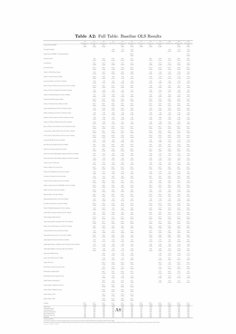
Table A2: Full Table: Baseline OLS Results(1) (2) (3) (4) (5) (6) (7) (8) (9) (10) (11) (12)

Ln(Credit Score) Ln(Credit Score) Ln(Credit Score) Ln(Credit Score) Ln(Credit Score) Ln(Credit Score) Ln(Credit Score) Ln(Credit Score) Ln(Credit Score) Ln(Credit Score) Ln(Credit Score) Ln(Credit Score)

Lagged Detrended DR007 0.04∗∗∗ 0.04∗∗∗ 0.04∗∗∗ 0.04∗∗∗ -0.05∗∗∗ 0.02∗∗∗ 0.01∗∗∗ 0.02∗∗∗ 0.02∗∗∗ -0.03∗∗

(0.000) (0.000) (0.000) (0.000) (0.001) (0.000) (0.000) (0.000) (0.000) (0.030)

Log Lagged Liquidity -0.39 -0.29 0.64∗ -0.19 -0.10 0.43

(0.213) (0.367) (0.072) (0.530) (0.748) (0.216)

Lagged Detrended DR007 × Log Lagged Liquidity 20.54∗∗∗ 11.47∗∗∗

(0.000) (0.000)

Log Loan Amount 0.22 1.27∗∗∗ 1.35∗∗∗ 1.23∗∗∗ 1.21∗∗∗ 0.90∗∗ 0.86∗∗ 0.87∗∗ 0.86∗∗ 0.85∗∗

(0.607) (0.002) (0.002) (0.005) (0.006) (0.019) (0.031) (0.039) (0.043) (0.043)

Loan Maturity -1.67∗∗∗ -1.82∗∗∗ -1.82∗∗∗ -1.81∗∗∗ -1.81∗∗∗ -1.82∗∗∗ -1.87∗∗∗ -1.87∗∗∗ -1.86∗∗∗ -1.86∗∗∗

(0.000) (0.000) (0.000) (0.000) (0.000) (0.000) (0.000) (0.000) (0.000) (0.000)

Loan Interest Rate -0.01∗∗∗ -0.01∗∗∗ -0.01∗∗∗ -0.01∗∗∗ -0.01∗∗∗ -0.01∗∗∗ -0.01∗∗∗ -0.01∗∗∗ -0.01∗∗∗ -0.01∗∗∗

(0.000) (0.000) (0.000) (0.000) (0.000) (0.000) (0.000) (0.000) (0.000) (0.000)

Number of Mobile Phone Carriers 0.00 -0.00∗∗ -0.00∗∗ -0.00∗∗ -0.00∗∗ -0.00 -0.00 -0.00 -0.00 -0.00

(0.537) (0.014) (0.025) (0.038) (0.044) (0.299) (0.162) (0.220) (0.238) (0.245)

Number of calls In the Past 3 Months -0.00∗∗∗ -0.00∗ -0.00 -0.00 -0.00 -0.00 -0.00 -0.00 -0.00 -0.00

(0.000) (0.097) (0.170) (0.146) (0.162) (0.118) (0.110) (0.183) (0.178) (0.191)

Longest Call Duration In The Past 12 Months -0.00 -0.00 -0.00 -0.00 -0.00 -0.00 -0.00 -0.00 -0.00 -0.00

(0.240) (0.471) (0.381) (0.463) (0.502) (0.312) (0.405) (0.363) (0.423) (0.454)

Ratio of Frequent Calls In Contact Book In the Past 12 Months -0.01∗∗∗ 0.00∗∗ 0.01∗∗ 0.01∗∗ 0.00∗∗ 0.00 0.00 0.00 0.00 0.00

(0.001) (0.032) (0.011) (0.026) (0.027) (0.849) (0.924) (0.592) (0.685) (0.649)

Number of Calls In the Black List In the Past 12 Months -0.00 -0.00 -0.00 -0.01 -0.01 0.00 0.00 -0.00 -0.00 -0.00

(0.943) (0.694) (0.189) (0.108) (0.113) (0.689) (0.875) (0.377) (0.323) (0.325)

Number of Calls With Family In the Past 12 Months 0.00 -0.00 -0.00 -0.00 -0.00 0.00 -0.00 -0.00 -0.00 -0.00

(0.602) (0.787) (0.570) (0.589) (0.604) (0.920) (0.870) (0.676) (0.694) (0.701)

Number of Calls With Agents As Caller -0.00∗∗∗ -0.00∗∗∗ -0.00∗∗∗ -0.00∗∗∗ -0.00∗∗∗ -0.00∗∗∗ -0.00∗∗∗ -0.00∗∗∗ -0.00∗∗∗ -0.00∗∗∗

(0.000) (0.002) (0.000) (0.000) (0.000) (0.004) (0.009) (0.002) (0.001) (0.001)

Number of Calls In the Past 3 Months As Caller 0.00∗∗∗ 0.00∗∗∗ 0.00∗∗∗ 0.00∗∗∗ 0.00∗∗∗ 0.00∗∗ 0.00∗∗ 0.00∗∗ 0.00∗∗ 0.00∗∗

(0.000) (0.004) (0.008) (0.006) (0.007) (0.019) (0.018) (0.031) (0.027) (0.028)

Longest Call Duration In The Past 12 Months As Caller -0.00 -0.00∗ -0.00∗∗ -0.00∗∗ -0.00∗∗ -0.00∗ -0.00∗ -0.00∗∗ -0.00∗∗ -0.00∗∗

(0.199) (0.072) (0.022) (0.032) (0.028) (0.057) (0.066) (0.026) (0.034) (0.031)

Median Call Duration In The Past 12 Months As Caller -0.00 -0.00 -0.00 -0.00 -0.00 -0.00 -0.00 -0.00 -0.00 -0.00

(0.227) (0.210) (0.469) (0.275) (0.287) (0.371) (0.349) (0.661) (0.461) (0.467)

Number of Calls To Agents in the Past 12 Months As Caller -0.00 -0.00 -0.00 -0.00 -0.00 -0.00 -0.00 -0.00 -0.00 -0.00

(0.293) (0.310) (0.319) (0.399) (0.430) (0.260) (0.371) (0.450) (0.481) (0.495)

Number of Calls In the Black List In the Past 12 Months -0.00 -0.00 0.00 0.01 0.00 -0.00 -0.00 0.00 0.00 0.00

(0.875) (0.991) (0.389) (0.285) (0.308) (0.492) (0.648) (0.716) (0.680) (0.695)

Ratio of Calls In Contact Book In the Past 12 Months As Caller 0.02∗∗∗ 0.01∗∗∗ 0.01∗∗∗ 0.01∗∗∗ 0.01∗∗∗ 0.01∗∗∗ 0.01∗∗∗ 0.01∗∗∗ 0.01∗∗∗ 0.01∗∗∗

(0.000) (0.000) (0.002) (0.001) (0.001) (0.000) (0.000) (0.000) (0.000) (0.000)

Average Times of Being Called Per Day In the Past 12 Months 0.00∗∗∗ 0.00∗∗∗ 0.00∗∗∗ 0.00∗∗∗ 0.00∗∗∗ 0.00∗∗∗ 0.00∗∗∗ 0.00∗∗∗ 0.00∗∗∗ 0.00∗∗∗

(0.000) (0.004) (0.008) (0.007) (0.008) (0.004) (0.004) (0.009) (0.008) (0.009)

Average Times of Being Caller Per Day In the Past 12 Months -0.00∗∗∗ -0.00∗∗∗ -0.00∗∗∗ -0.00∗∗∗ -0.00∗∗∗ -0.00∗∗∗ -0.00∗∗∗ -0.00∗∗∗ -0.00∗∗∗ -0.00∗∗∗

(0.000) (0.000) (0.000) (0.000) (0.000) (0.000) (0.001) (0.001) (0.001) (0.001)

Average Mobile Bill In the Past 12 Months -0.00 -0.00 -0.00 -0.00 -0.00 -0.00 -0.00∗ -0.00 -0.00 -0.00

(0.167) (0.234) (0.266) (0.200) (0.184) (0.372) (0.090) (0.123) (0.121) (0.119)

Have Shortcuts for Family In the Past 12 Months 0.00∗ 0.00∗∗ 0.00∗∗ 0.00∗∗ 0.00∗∗ 0.00∗ 0.00∗ 0.00∗∗ 0.00∗∗ 0.00∗∗

(0.057) (0.029) (0.020) (0.027) (0.028) (0.055) (0.052) (0.041) (0.048) (0.048)

Number of the Contacts In The Contact Book 0.00∗∗∗ 0.00∗∗∗ 0.00∗∗∗ 0.00∗∗∗ 0.00∗∗∗ 0.00∗∗∗ 0.00∗∗∗ 0.00∗∗∗ 0.00∗∗∗ 0.00∗∗∗

(0.000) (0.000) (0.000) (0.000) (0.000) (0.000) (0.000) (0.000) (0.000) (0.000)

Transaction Amount With Trading Companies In The Past 12 Months 0.00 0.00 0.00 0.00 0.00 0.00 0.00 0.00 0.00 0.00

(0.617) (0.177) (0.201) (0.205) (0.185) (0.210) (0.151) (0.177) (0.182) (0.169)

Transaction Number With Trading Companies In The Past 12 Months 0.00 -0.00 -0.00 -0.00 -0.00 -0.00 -0.00 -0.00 -0.00 -0.00

(0.980) (0.375) (0.504) (0.532) (0.561) (0.280) (0.249) (0.380) (0.397) (0.410)

Number of Active Credit Cards 0.00 0.00 0.00 0.00 0.00 0.00 0.00 0.00 0.00 0.00

(0.628) (0.286) (0.286) (0.272) (0.314) (0.533) (0.494) (0.445) (0.429) (0.452)

Number of Banks of the Credit Cards 0.00∗∗∗ 0.00∗∗∗ 0.00∗∗∗ 0.00∗∗∗ 0.00∗∗∗ 0.00∗∗∗ 0.00∗∗∗ 0.00∗∗∗ 0.00∗∗∗ 0.00∗∗∗

(0.000) (0.000) (0.000) (0.000) (0.000) (0.000) (0.000) (0.000) (0.000) (0.000)

Number of Cash Withdrawal in the Past 12 Months -0.00 0.00 0.00 0.00 0.00 0.00 0.00 0.00 0.00 0.00

(0.466) (0.815) (0.534) (0.576) (0.558) (0.886) (0.755) (0.441) (0.459) (0.452)

Total Interest Charged In the Past 6 Months -0.00 0.00 0.00∗ 0.00∗ 0.00∗ 0.00∗∗ 0.00∗ 0.00∗∗ 0.00∗∗ 0.00∗∗

(0.862) (0.105) (0.072) (0.094) (0.078) (0.045) (0.053) (0.033) (0.044) (0.039)

Number of Interest Charged In the Past 12 Months 0.00∗∗∗ 0.00∗∗∗ 0.00∗∗ 0.00∗∗ 0.00∗∗ 0.00∗ 0.00∗ 0.00∗ 0.00∗ 0.00∗

(0.000) (0.006) (0.012) (0.012) (0.013) (0.078) (0.052) (0.078) (0.077) (0.079)

Number of Transactions Over 5000 RMB in the Past 12 Months 0.00∗∗∗ 0.00∗∗ 0.00∗∗ 0.00∗∗ 0.00∗∗ 0.00∗∗∗ 0.00∗∗ 0.00∗∗ 0.00∗∗ 0.00∗∗

(0.003) (0.022) (0.047) (0.046) (0.047) (0.007) (0.012) (0.027) (0.027) (0.028)

Highest Credit Line in the Past 12 Months 0.00∗∗∗ 0.00∗ 0.00∗ 0.00∗ 0.00∗ 0.00 0.00 0.00 0.00 0.00

(0.000) (0.091) (0.072) (0.056) (0.062) (0.100) (0.273) (0.230) (0.199) (0.206)

Repayment Rate in the Past 6 Months 0.00∗∗∗ 0.00∗∗∗ 0.00∗∗∗ 0.00∗∗∗ 0.00∗∗∗ 0.00∗∗∗ 0.00∗∗∗ 0.00∗∗ 0.00∗∗ 0.00∗∗

(0.004) (0.002) (0.005) (0.003) (0.002) (0.004) (0.009) (0.019) (0.011) (0.010)

Minimum Repayment Rate in the Past 12 Months -0.00 -0.00∗∗ -0.00 -0.00 -0.00 -0.00 -0.00 -0.00 -0.00 -0.00

(0.113) (0.029) (0.129) (0.119) (0.118) (0.136) (0.171) (0.381) (0.352) (0.344)

Usage Rate of Credit Line in the Past 6 Months -0.00∗∗∗ -0.01∗∗∗ -0.01∗∗∗ -0.01∗∗∗ -0.01∗∗∗ -0.01∗∗∗ -0.01∗∗∗ -0.01∗∗∗ -0.01∗∗∗ -0.01∗∗∗

(0.003) (0.000) (0.000) (0.000) (0.000) (0.000) (0.000) (0.000) (0.000) (0.000)

Number Of Bank Relationship In The Past 3 Months -0.00 -0.00∗∗ -0.00 -0.00∗ -0.00∗ -0.00∗∗ -0.00∗∗∗ -0.00∗∗ -0.00∗∗ -0.00∗∗

(0.180) (0.022) (0.126) (0.099) (0.088) (0.016) (0.006) (0.041) (0.034) (0.033)

Number Of Active Deposit Cards In The Past 3 Months 0.00∗ 0.00∗∗ 0.00∗ 0.00∗ 0.00∗ 0.00∗∗ 0.00∗∗ 0.00∗∗ 0.00∗∗ 0.00∗∗

(0.097) (0.034) (0.087) (0.069) (0.058) (0.018) (0.015) (0.035) (0.031) (0.029)

Online Shopping Address Entropy 0.01∗∗∗ 0.01∗∗∗ 0.01∗∗∗ 0.01∗∗∗ 0.01∗∗∗ 0.01∗∗∗ 0.01∗∗∗ 0.01∗∗∗ 0.01∗∗∗ 0.01∗∗∗

(0.000) (0.000) (0.000) (0.000) (0.000) (0.000) (0.000) (0.000) (0.000) (0.000)

Alipay Average Daily Consumption in The Past 12 Months 0.00∗∗∗ 0.01∗∗∗ 0.00∗∗∗ 0.00∗∗∗ 0.00∗∗∗ 0.01∗∗∗ 0.01∗∗∗ 0.00∗∗∗ 0.00∗∗∗ 0.00∗∗∗

(0.009) (0.001) (0.007) (0.005) (0.004) (0.000) (0.000) (0.002) (0.002) (0.001)

Alipay Average Daily Transaction in The Past 12 Months -0.00∗∗ -0.00∗∗∗ -0.00∗∗ -0.00∗∗ -0.00∗∗ -0.00∗∗∗ -0.00∗∗∗ -0.00∗∗∗ -0.00∗∗∗ -0.00∗∗∗

(0.017) (0.004) (0.014) (0.013) (0.013) (0.000) (0.000) (0.002) (0.002) (0.002)

Average Transfer Per Day In the Past 12 Months 0.00 0.00∗ 0.00∗ 0.00∗ 0.00∗ 0.00∗∗ 0.00∗∗ 0.00∗∗ 0.00∗∗ 0.00∗∗

(0.430) (0.059) (0.057) (0.092) (0.088) (0.011) (0.018) (0.020) (0.027) (0.027)

Alipay Gamble Transaction Fees in The Past 12 Months -0.00∗∗ -0.00∗∗ -0.00∗∗ -0.00∗∗ -0.00∗ -0.00∗∗∗ -0.00∗∗∗ -0.00∗∗∗ -0.00∗∗∗ -0.00∗∗∗

(0.021) (0.035) (0.022) (0.036) (0.059) (0.000) (0.000) (0.000) (0.000) (0.000)

Alipay Implied Credit Lines In The Past 12 Months 0.00 0.00 -0.00 0.00 0.00 0.00 0.00 0.00 0.00 0.00

(0.434) (0.975) (0.946) (0.978) (0.933) (0.542) (0.548) (0.645) (0.620) (0.600)

Alipay Implied Number of Banks of Credit Cards In The Past 12 Months -0.00 -0.00 -0.00 -0.00 -0.00 -0.00∗ -0.00∗ -0.00 -0.00 -0.00

(0.111) (0.290) (0.568) (0.477) (0.437) (0.060) (0.092) (0.240) (0.215) (0.205)

Alipay Implied Highest Credit Line In The Past 12 Months -0.00∗∗ -0.00 -0.00 -0.00 -0.00 -0.00∗ -0.00∗ -0.00 -0.00∗ -0.00∗

(0.038) (0.208) (0.245) (0.214) (0.188) (0.059) (0.082) (0.101) (0.099) (0.091)

Lagged Stock Market Return 0.04 -0.54 -0.20 -0.50 -0.54 -0.79 -0.62 -0.77

(0.940) (0.306) (0.704) (0.343) (0.281) (0.124) (0.229) (0.135)

Lagged Stock Market Return for SMEs -0.30 0.66∗ -0.35 -0.08 0.14 0.64∗ 0.11 0.24

(0.413) (0.065) (0.351) (0.834) (0.699) (0.072) (0.764) (0.515)

Lagged Yield Curve 0.02∗∗∗ 0.02∗∗∗ 0.02∗∗∗ 0.02∗∗∗ 0.01∗∗∗ 0.00 0.01∗∗∗ 0.01∗∗

(0.000) (0.000) (0.000) (0.000) (0.003) (0.313) (0.005) (0.015)

P2P Industry Loan Rate Composite Index 0.70∗ 2.44∗∗∗ 1.43∗∗∗ 1.52∗∗∗ 0.58 1.33∗∗∗ 0.82∗ 0.90∗∗

(0.061) (0.000) (0.001) (0.000) (0.131) (0.002) (0.055) (0.037)

P2P Industry Popularity Index 0.08∗∗∗ 0.10∗∗∗ 0.08∗∗∗ 0.07∗∗∗ 0.03∗ 0.04∗∗ 0.03∗ 0.03

(0.000) (0.000) (0.000) (0.001) (0.056) (0.022) (0.074) (0.169)

P2P Industry Investor Composite Return 0.65 0.86 -1.06 -0.67 -2.06 -2.20 -2.57 -2.43

(0.695) (0.624) (0.547) (0.704) (0.222) (0.226) (0.156) (0.178)

Lagged Change in Housing Price -0.20∗∗ -0.13 -0.17∗∗ -0.15∗ -0.14 -0.12 -0.13 -0.13

(0.014) (0.102) (0.044) (0.060) (0.117) (0.168) (0.156) (0.153)

Lagged Change in Banking Total Assets 0.05∗∗∗ 0.05∗∗∗ 0.05∗∗∗ 0.05∗∗∗

(0.000) (0.000) (0.000) (0.000)

Lagged Change in Banking Leverage -0.25∗∗∗ -0.28∗∗∗ -0.27∗∗∗ -0.28∗∗∗

(0.000) (0.000) (0.000) (0.000)

Lagged Change in PMI -0.01∗∗∗ -0.01∗∗∗ -0.01∗∗∗ -0.01∗∗∗

(0.000) (0.000) (0.000) (0.000)

Lagged Change in CPI -0.02∗∗∗ -0.02∗∗∗ -0.02∗∗∗ -0.02∗∗∗

(0.000) (0.000) (0.000) (0.000)

Constant 6.47∗∗∗ 6.55∗∗∗ 6.44∗∗∗ 6.37∗∗∗ 6.43∗∗∗ 6.41∗∗∗ 6.47∗∗∗ 6.56∗∗∗ 6.56∗∗∗ 6.53∗∗∗ 6.56∗∗∗ 6.55∗∗∗

(0.000) (0.000) (0.000) (0.000) (0.000) (0.000) (0.000) (0.000) (0.000) (0.000) (0.000) (0.000)

Observations 11956 11956 10953 10008 9922 9922 11956 11956 10953 10008 9922 9922

Adjusted R-Squared 0.02 0.59 0.66 0.65 0.66 0.66 0.12 0.68 0.69 0.69 0.68 0.68

Loan Characteristics NO YES YES YES YES YES NO YES YES YES YES YES

Borrower Characteristics NO YES YES YES YES YES NO YES YES YES YES YES

Macro Characteristics NO NO YES YES YES YES NO NO YES YES YES YES

Borrower Province FE YES YES YES YES YES YES YES YES YES YES YES YES

Month FE NO NO NO NO NO NO YES YES YES YES YES YES

p-values in parentheses

In this table the independent variable of Log Lagged Liquidity, Log Loan Amount, Loan Maturity, Lagged Stock Market Return, Lagged Stock Market Return for SMES,

P2P Industry Loan Rate Composite Index, P2P Industry Popularity Index, P2P Industry Investor Composite Return, Lagged Change in Housing Price and Lagged CHange in Banking Total Assets are rescaled by 10−3 times original value, for clear presentation of the estimates.

∗ p < 0.1, ∗∗ p < 0.05, ∗∗∗ p < 0.01

A8

Table A3: Full Table: Baseline OLS Results Using Overdue History to Replace Credit ScoreNumber of Overdue(6M) Amount of Overdue(6M) Number of Overdue Ratio(3M to 9M)

(1) (2) (3) (4) (5) (6) (7) (8) (9)

Lagged Detrended DR007 -367.26∗∗∗ -353.93∗∗∗ -874.39∗ -52.89∗ -47.53 -182.52∗ -685.49∗∗∗ -712.15∗∗∗ -1692.12

(0.002) (0.006) (0.059) (0.068) (0.133) (0.053) (0.006) (0.008) (0.129)

Log Lagged Liquidity 16.95∗ 22.37∗∗ 3.22∗∗ 4.63∗∗∗ -14.10 -3.90

(0.091) (0.046) (0.047) (0.009) (0.583) (0.881)

Lagged Detrended DR007 × Log Lagged Liquidity 117.39 30.45 221.04

(0.247) (0.102) (0.358)

Log Loan Amount 42.45∗∗∗ 41.34∗∗ 41.32∗∗ 11.92∗∗∗ 12.24∗∗∗ 12.24∗∗∗ 8.07 6.82 6.78

(0.007) (0.017) (0.017) (0.002) (0.005) (0.005) (0.747) (0.800) (0.801)

Loan Maturity 3.71∗∗ 4.29∗∗ 4.29∗∗ -0.10 -0.02 -0.02 -1.32 -1.29 -1.29

(0.040) (0.027) (0.027) (0.804) (0.963) (0.964) (0.720) (0.745) (0.745)

Loan Interest Rate 3.30∗∗ 3.11∗∗ 3.11∗∗ 0.45 0.45 0.45 0.74 0.48 0.48

(0.019) (0.032) (0.033) (0.110) (0.121) (0.122) (0.798) (0.873) (0.875)

Number of Mobile Phone Carriers -13.62 -17.71 -17.62 -7.72∗∗∗ -8.79∗∗∗ -8.77∗∗∗ -19.23 -20.98 -20.82

(0.233) (0.160) (0.162) (0.002) (0.002) (0.002) (0.213) (0.209) (0.213)

Number of calls In the Past 3 Months 0.09 0.07 0.07 0.03∗ 0.03∗ 0.03∗ 0.03 -0.03 -0.03

(0.185) (0.301) (0.294) (0.073) (0.091) (0.087) (0.817) (0.811) (0.823)

Longest Call Duration In The Past 12 Months 0.00∗∗ 0.00∗∗ 0.00∗∗ 0.00 0.00 0.00 -0.00 -0.00 -0.00

(0.023) (0.022) (0.022) (0.277) (0.408) (0.342) (0.813) (0.725) (0.745)

Ratio of Frequent Calls In Contact Book In the Past 12 Months -78.94 -59.62 -58.49 5.42 9.28 9.57 -80.72 -52.94 -50.80

(0.289) (0.440) (0.450) (0.710) (0.548) (0.537) (0.556) (0.721) (0.732)

Number of Calls In the Black List In the Past 12 Months -75.32 -74.50 -74.35 3.34 3.67 3.71 -369.25 -245.30∗ -245.02∗

(0.149) (0.144) (0.144) (0.430) (0.665) (0.660) (0.114) (0.095) (0.095)

Number of Calls With Family In the Past 12 Months -0.03∗∗ -0.03∗ -0.03∗ -0.01∗∗∗ -0.01∗∗ -0.01∗∗ -0.06∗ -0.05 -0.05

(0.035) (0.077) (0.078) (0.006) (0.011) (0.011) (0.055) (0.120) (0.120)

Number of Calls With Agents As Caller 0.05 0.07 0.07 -0.01 -0.01 -0.01 0.25 0.32 0.32

(0.702) (0.637) (0.627) (0.615) (0.637) (0.653) (0.673) (0.613) (0.609)

Number of Calls In the Past 3 Months As Caller -0.14 -0.13 -0.13 -0.07∗ -0.07 -0.07 0.00 0.09 0.09

(0.303) (0.367) (0.363) (0.097) (0.109) (0.107) (0.995) (0.734) (0.740)

Longest Call Duration In The Past 12 Months As Caller 0.01∗ 0.01 0.01 -0.00 -0.00 -0.00 0.02∗∗ 0.02∗ 0.02∗

(0.056) (0.137) (0.140) (0.965) (0.673) (0.662) (0.043) (0.071) (0.073)

Median Call Duration In The Past 12 Months As Caller -0.81 -0.88 -0.88 0.02 0.01 0.01 -1.03 -0.88 -0.87

(0.111) (0.103) (0.103) (0.789) (0.912) (0.908) (0.384) (0.491) (0.493)

Number of Calls To Agents in the Past 12 Months As Caller -0.45 -0.37 -0.37 -0.07 -0.07 -0.06 -0.34 -0.21 -0.20

(0.153) (0.264) (0.269) (0.429) (0.500) (0.506) (0.587) (0.752) (0.760)

Number of Calls In the Black List In the Past 12 Months 151.47 148.83 148.00 -7.96 -9.02 -9.24 801.25 663.09∗∗ 661.53∗∗

(0.187) (0.118) (0.121) (0.355) (0.475) (0.462) (0.123) (0.047) (0.048)

Ratio of Calls In Contact Book In the Past 12 Months As Caller -3.86 -43.26 -44.40 -3.13 -7.88 -8.18 -49.19 -54.36 -56.49

(0.966) (0.654) (0.645) (0.864) (0.695) (0.684) (0.754) (0.745) (0.735)

Average Times of Being Called Per Day In the Past 12 Months -3.42 -1.35 -1.43 -1.78 -1.73 -1.75 -3.79 0.81 0.65

(0.561) (0.836) (0.826) (0.320) (0.390) (0.383) (0.768) (0.954) (0.963)

Average Times of Being Caller Per Day In the Past 12 Months 5.58 5.33 5.29 3.41 3.62 3.61 1.57 -1.29 -1.36

(0.475) (0.530) (0.533) (0.179) (0.190) (0.191) (0.903) (0.927) (0.923)

Average Mobile Bill In the Past 12 Months 0.20∗ 0.18 0.18 -0.01 -0.01 -0.01 -0.26 -0.25 -0.25

(0.077) (0.126) (0.127) (0.722) (0.649) (0.647) (0.198) (0.251) (0.250)

Have Shortcuts for Family In the Past 12 Months -31.54 -31.61 -31.67 0.01 -2.27 -2.29 109.80 125.57 125.45

(0.262) (0.292) (0.290) (0.998) (0.712) (0.710) (0.128) (0.107) (0.107)

Number of the Contacts In The Contact Book 0.02 0.02 0.02 0.00 0.00 0.00 0.02 0.01 0.01

(0.142) (0.163) (0.164) (0.795) (0.996) (1.000) (0.708) (0.848) (0.850)

Transaction Amount With Trading Companies In The Past 12 Months 0.00 0.00 0.00 0.00 0.00 0.00 0.00 0.00 0.00

(0.174) (0.225) (0.220) (0.432) (0.407) (0.403) (0.474) (0.399) (0.390)

Transaction Number With Trading Companies In The Past 12 Months -1.72∗∗∗ -1.64∗∗ -1.64∗∗ -0.39∗∗ -0.42∗∗ -0.42∗∗ -1.36∗ -1.50∗ -1.48∗

(0.003) (0.010) (0.010) (0.041) (0.048) (0.049) (0.075) (0.068) (0.070)

Number of Active Credit Cards 2.86 3.49 3.45 -0.79 -0.96 -0.97 0.43 0.09 0.00

(0.472) (0.489) (0.495) (0.201) (0.226) (0.219) (0.928) (0.988) (1.000)

Number of Banks of the Credit Cards 10.51 9.96 10.00 0.79 1.02 1.03 19.61∗∗ 21.59∗∗ 21.65∗∗

(0.166) (0.257) (0.256) (0.766) (0.724) (0.722) (0.042) (0.042) (0.041)

Number of Cash Withdrawal in the Past 12 Months 0.81 0.86 0.87 0.37 0.39 0.39 -0.44 -0.45 -0.45

(0.251) (0.243) (0.243) (0.172) (0.170) (0.170) (0.418) (0.432) (0.434)

Total Interest Charged In the Past 6 Months -0.00 -0.00 -0.00 -0.00 -0.00 -0.00 0.00 0.00 0.00

(0.142) (0.182) (0.187) (0.216) (0.201) (0.206) (0.587) (0.731) (0.721)

Number of Interest Charged In the Past 12 Months 0.82∗∗ 0.71 0.70 -0.10 -0.12 -0.12 0.37 0.48 0.48

(0.045) (0.112) (0.112) (0.448) (0.390) (0.389) (0.657) (0.597) (0.598)

Number of Transactions Over 5000 RMB in the Past 12 Months 0.59∗ 0.62∗ 0.62∗ 0.36 0.37 0.37 0.36 0.38 0.38

(0.092) (0.091) (0.092) (0.110) (0.104) (0.105) (0.280) (0.271) (0.276)

Highest Credit Line in the Past 12 Months -0.00∗∗∗ -0.00∗∗∗ -0.00∗∗∗ -0.00 -0.00 -0.00 -0.00 -0.00 -0.00

(0.005) (0.009) (0.009) (0.872) (0.914) (0.911) (0.659) (0.752) (0.746)

Repayment Rate in the Past 6 Months -24.99 -26.68 -26.37 -7.50 -9.15 -9.07 6.51 -7.86 -7.27

(0.590) (0.589) (0.594) (0.598) (0.541) (0.545) (0.929) (0.920) (0.926)

Minimum Repayment Rate in the Past 12 Months -75.26∗∗ -85.93∗∗ -86.10∗∗ -22.13∗∗ -22.89∗∗ -22.94∗∗ 30.80 28.50 28.17

(0.034) (0.025) (0.025) (0.013) (0.020) (0.019) (0.594) (0.646) (0.650)

Usage Rate of Credit Line in the Past 6 Months 55.52 44.56 43.74 -9.71 -10.74 -10.95 22.89 17.99 16.43

(0.261) (0.396) (0.405) (0.637) (0.618) (0.610) (0.771) (0.827) (0.842)

Number Of Bank Relationship In The Past 3 Months 8.72 7.35 7.16 -2.44 -2.08 -2.13 -9.46 -15.59 -15.95

(0.809) (0.852) (0.856) (0.802) (0.848) (0.845) (0.854) (0.782) (0.778)

Number Of Active Deposit Cards In The Past 3 Months -8.95 -8.76 -8.51 -4.08 -4.45 -4.39 -20.98 -21.89 -21.43

(0.726) (0.757) (0.764) (0.602) (0.604) (0.610) (0.579) (0.603) (0.611)

Online Shopping Address Entropy 26.13 30.45 30.49 13.74 15.70 15.71 57.31 38.86 38.94

(0.560) (0.527) (0.527) (0.239) (0.225) (0.225) (0.479) (0.652) (0.651)

Alipay Average Daily Consumption in The Past 12 Months -12.28 -10.12 -9.64 -1.36 -0.90 -0.77 18.55 18.66 19.56

(0.694) (0.753) (0.764) (0.854) (0.906) (0.919) (0.767) (0.775) (0.764)

Alipay Average Daily Transaction in The Past 12 Months 1.00 0.44 0.48 1.25 0.84 0.85 -5.57 -5.33 -5.25

(0.947) (0.977) (0.975) (0.650) (0.766) (0.763) (0.791) (0.807) (0.809)

Average Transfer Per Day In the Past 12 Months -0.02∗∗ -0.02∗∗ -0.02∗∗ -0.01∗ -0.01∗ -0.01∗ -0.03∗∗∗ -0.03∗∗ -0.03∗∗

(0.029) (0.028) (0.028) (0.062) (0.070) (0.070) (0.008) (0.015) (0.015)

Alipay Gamble Transaction Fees in The Past 12 Months 0.04∗∗∗ 0.04∗∗∗ 0.04∗∗∗ 0.01∗∗∗ 0.01∗∗∗ 0.01∗∗∗ 0.03∗∗ 0.03∗∗ 0.03∗∗

(0.000) (0.000) (0.000) (0.000) (0.000) (0.000) (0.029) (0.033) (0.032)

Alipay Implied Credit Lines In The Past 12 Months 0.01 0.01 0.01 0.00 0.00 0.00 0.00 0.01 0.01

(0.134) (0.123) (0.121) (0.369) (0.364) (0.360) (0.441) (0.339) (0.336)

Alipay Implied Number of Banks of Credit Cards In The Past 12 Months -0.32 3.11 2.97 3.99 4.99 4.95 -8.73 -12.96 -13.22

(0.988) (0.894) (0.899) (0.405) (0.334) (0.337) (0.783) (0.709) (0.704)

Alipay Implied Highest Credit Line In The Past 12 Months -0.01 -0.01 -0.01 -0.00 -0.00 -0.00 -0.01∗ -0.02∗∗ -0.02∗∗

(0.402) (0.378) (0.375) (0.352) (0.302) (0.298) (0.065) (0.030) (0.029)

Lagged Stock Market Return -4.82 -2.00 -3.54 1.50 2.51 2.10 33.97 26.40 23.49

(0.792) (0.915) (0.851) (0.625) (0.432) (0.511) (0.253) (0.389) (0.450)

Lagged Stock Market Return for SMEs 35.38∗∗ 31.42∗∗ 32.78∗∗ 6.31∗∗ 5.84∗∗ 6.19∗∗ 19.54 22.98 25.53

(0.014) (0.032) (0.026) (0.018) (0.035) (0.027) (0.338) (0.270) (0.230)

Lagged Yield Curve -45.08 -32.16 -42.39 -22.03 -19.85 -22.50 -218.59 -258.28 -277.54

(0.623) (0.746) (0.673) (0.217) (0.309) (0.255) (0.216) (0.175) (0.151)

P2P Industry Loan Rate Composite Index 7.68 14.79 15.57 3.56 3.83 4.03 21.50 48.01 49.46

(0.468) (0.263) (0.242) (0.121) (0.181) (0.157) (0.367) (0.115) (0.104)

P2P Industry Popularity Index -0.50 -0.64 -0.72 -0.10 -0.14 -0.16 -1.01 -0.45 -0.59

(0.342) (0.255) (0.204) (0.351) (0.203) (0.145) (0.364) (0.708) (0.621)

P2P Industry Investor Composite Return -37.28 -53.57 -52.14 -21.72∗ -23.11∗ -22.74∗ -107.05 -164.49 -161.81

(0.457) (0.334) (0.347) (0.070) (0.084) (0.090) (0.368) (0.224) (0.233)

Lagged Change in Housing Price 0.99 1.68 1.68 -0.75 -0.75 -0.75 4.47 3.19 3.18

(0.760) (0.611) (0.613) (0.393) (0.402) (0.401) (0.274) (0.446) (0.448)

Constant -272.46 -419.54 -485.81 -41.90 -48.96 -66.15 1082.60 580.47 455.69

(0.552) (0.399) (0.343) (0.673) (0.644) (0.548) (0.217) (0.540) (0.638)

Observations 10953 9922 9922 10953 9922 9922 10953 9922 9922

Adjusted R-Squared 0.03 0.03 0.03 0.06 0.07 0.07 0.01 0.01 0.01

Loan Characteristics YES YES YES YES YES YES YES YES YES

Borrower Characteristics YES YES YES YES YES YES YES YES YES

Macro Characteristics YES YES YES YES YES YES YES YES YES

Province FE YES YES YES YES YES YES YES YES YES

Month FE YES YES YES YES YES YES YES YES YES

p-values in parentheses

In this table the dependent variable of Number of Overdue (6M) and Number of Overdue Ratio(3M to 9M) are rescaled by 1000 times original value, for clear presentation of the estimates.

∗ p < 0.1, ∗∗ p < 0.05, ∗∗∗ p < 0.01

A9

Table A4: Full Table: Baseline Probit Model Results(1) (2) (3) (4) (5) (6) (7)

Granted Granted Granted Granted Granted Granted Granted

Granted

Lagged Detrended DR007 -0.14∗∗ -36.30∗∗∗ -93.67∗∗ -83.15∗ -87.73∗∗ -74.95∗

(0.026) (0.000) (0.027) (0.051) (0.041) (0.085)

Ln(Credit Score) 5.33∗∗∗ 8.56∗∗∗ 8.76∗∗∗ 8.38∗∗∗ 7.80∗∗∗ 8.15∗∗∗

(0.000) (0.000) (0.000) (0.000) (0.000) (0.000)

Lagged Detrended DR007 × Ln(Credit Score) 5.58∗∗∗ 14.37∗∗ 12.72∗ 13.44∗∗ 11.64∗

(0.000) (0.028) (0.054) (0.043) (0.084)

Lagged Liquidity 4.65∗∗∗ 4.79∗∗∗ 4.84∗∗∗ 4.36∗∗∗ 2.96∗∗∗

(0.000) (0.000) (0.000) (0.000) (0.001)

Lagged Liquidity × Ln(Credit Score) -0.71∗∗∗ -0.73∗∗∗ -0.74∗∗∗ -0.67∗∗∗ -0.46∗∗∗

(0.000) (0.000) (0.000) (0.000) (0.001)

Lagged Detrended DR007 × Lagged Liquidity 13.48 10.92 12.90 14.32

(0.150) (0.248) (0.175) (0.137)

Lagged Detrended DR007 × Ln(Credit Score) × Lagged Liquidity -2.07 -1.67 -1.97 -2.24

(0.154) (0.255) (0.180) (0.134)

Log Loan Amount -0.19∗∗∗ -0.25∗∗∗ -0.27∗∗∗

(0.000) (0.000) (0.000)

Loan Maturity -0.03∗∗∗ -0.03∗∗∗ -0.02∗∗∗

(0.000) (0.000) (0.000)

Loan Interest Rate -0.01∗∗∗ -0.01∗∗∗ -0.01∗∗∗

(0.000) (0.000) (0.001)

Male 0.01 0.03∗

(0.376) (0.062)

Age 0.01∗∗∗ 0.01∗∗∗

(0.000) (0.000)

Number of Mobile Phone Carriers -0.05∗∗∗ -0.03∗∗∗

(0.000) (0.000)

Number of calls In the Past 3 Months -0.00∗∗ -0.00

(0.012) (0.102)

Longest Call Duration In The Past 12 Months -0.00 -0.00

(0.566) (0.513)

Ratio of Frequent Calls In Contact Book In the Past 12 Months 0.22∗∗∗ 0.17∗∗∗

(0.000) (0.000)

Number of Calls In the Black List In the Past 12 Months 0.02 0.01

(0.458) (0.690)

Number of Calls With Family In the Past 12 Months -0.00 -0.00

(0.138) (0.143)

Number of Calls With Agents As Caller -0.00∗∗∗ -0.00∗∗∗

(0.000) (0.000)

Number of Calls In the Past 3 Months As Caller 0.00∗∗ 0.00

(0.033) (0.231)

Longest Call Duration In The Past 12 Months As Caller 0.00∗∗∗ 0.00∗∗∗

(0.002) (0.004)

Median Call Duration In The Past 12 Months As Caller -0.00∗∗∗ -0.00∗∗∗

(0.000) (0.000)

Number of Calls To Agents in the Past 12 Months As Caller -0.00∗∗∗ -0.00∗∗∗

(0.000) (0.000)

Number of Calls In the Black List In the Past 12 Months -0.04 -0.04

(0.188) (0.224)

Ratio of Calls In Contact Book In the Past 12 Months As Caller 0.24∗∗∗ 0.39∗∗∗

(0.000) (0.000)

Average Times of Being Called Per Day In the Past 12 Months 0.00 0.00

(0.324) (0.491)

Average Times of Being Caller Per Day In the Past 12 Months -0.00 -0.00

(0.272) (0.716)

Average Mobile Bill In the Past 12 Months 0.00 -0.00

(0.670) (0.753)

Have Shortcuts for Family In the Past 12 Months -0.04∗∗ -0.05∗∗

(0.041) (0.019)

Number of the Contacts In The Contact Book -0.00∗∗∗ -0.00∗∗∗

(0.000) (0.000)

Transaction Amount With Trading Companies In The Past 12 Months 0.00∗ 0.00

(0.055) (0.200)

Transaction Number With Trading Companies In The Past 12 Months -0.00 -0.00

(0.527) (0.670)

Number of Active Credit Cards -0.02∗∗∗ -0.02∗∗∗

(0.000) (0.000)

Number of Banks of the Credit Cards 0.02∗∗∗ 0.02∗∗∗

(0.000) (0.001)

Number of Cash Withdrawal in the Past 12 Months 0.00 0.00

(0.158) (0.112)

Total Interest Charged In the Past 6 Months 0.00∗∗∗ 0.00∗∗∗

(0.000) (0.000)

Number of Interest Charged In the Past 12 Months -0.00∗∗∗ -0.00∗∗∗

(0.000) (0.000)

Number of Transactions Over 5000 RMB in the Past 12 Months 0.00 0.00∗∗

(0.112) (0.045)

Highest Credit Line in the Past 12 Months 0.00∗∗∗ 0.00∗∗∗

(0.000) (0.000)

Repayment Rate in the Past 6 Months 0.11∗∗∗ 0.11∗∗∗

(0.000) (0.000)

Minimum Repayment Rate in the Past 12 Months 0.05∗∗ 0.04∗

(0.031) (0.076)

Usage Rate of Credit Line in the Past 6 Months -0.37∗∗∗ -0.31∗∗∗

(0.000) (0.000)

Number Of Bank Relationship In The Past 3 Months -0.11∗∗∗ -0.10∗∗∗

(0.000) (0.000)

Number Of Active Deposit Cards In The Past 3 Months 0.03∗∗ 0.02

(0.020) (0.242)

Online Shopping Address Entropy -0.01 -0.01

(0.738) (0.800)

Alipay Average Daily Consumption in The Past 12 Months -0.02 -0.02

(0.266) (0.367)

Alipay Average Daily Transaction in The Past 12 Months 0.00 0.00

(0.751) (0.939)

Average Transfer Per Day In the Past 12 Months 0.00 0.00

(0.771) (0.671)

Alipay Gamble Transaction Fees in The Past 12 Months 0.00 0.00

(0.809) (0.767)

Alipay Implied Credit Lines In The Past 12 Months -0.00 0.00

(0.745) (0.766)

Alipay Implied Number of Banks of Credit Cards In The Past 12 Months -0.01 -0.01

(0.438) (0.480)

Alipay Implied Highest Credit Line In The Past 12 Months 0.00 0.00

(0.168) (0.449)

Lagged Change in Housing Price 0.01∗∗∗

(0.001)

Lagged Change in Banking Total Assets -0.00∗∗∗

(0.000)

Lagged Change in Banking Leverage 3.45∗∗∗

(0.000)

Lagged Stock Market Return -0.04∗∗∗

(0.000)

Lagged Stock Market Return for SMEs 0.01∗

(0.092)

Lagged Yield Curve 0.06

(0.217)

P2P Industry Loan Rate Composite Index -0.02∗

(0.077)

P2P Industry Popularity Index 0.00

(0.167)

P2P Industry Investor Composite Return 0.01

(0.725)

Lagged Change in PMI 0.21∗∗∗

(0.000)

Lagged Change in CPI 0.46∗∗∗

(0.000)

Constant -0.92∗∗∗ -35.32∗∗∗ -56.49∗∗∗ -57.76∗∗∗ -53.02∗∗∗ -48.85∗∗∗ -49.29∗∗∗

(0.000) (0.000) (0.000) (0.000) (0.000) (0.000) (0.000)

Observations 72861 72861 66639 66236 66236 66236 54113

Loan Characteristics NO NO NO NO YES YES YES

Borrower Characteristics NO NO NO NO NO YES YES

Macro Characteristics NO NO NO NO NO NO YES

Borrower FE NO NO NO NO NO NO NO

Time FE NO NO NO NO NO NO NO

p-values in parentheses

∗ p < 0.1, ∗∗ p < 0.05, ∗∗∗ p < 0.01

A10

Table A5: Consecutive Days of Low Monetary Policy

(1) (2)

OLS Model Probit Model

Ln(Credit Score) 9.0778∗∗∗

(0.000)

Days of Consecutive Low Monetary Policy 3.4286∗∗

(0.017)

Log Lagged Liquidity 4529.6841∗∗∗

(0.000)

Days of Consecutive Low Monetary Policy=1 -0.0022∗∗

(0.020)

Days of Consecutive Low Monetary Policy=2 -0.0029∗∗

(0.017)

Days of Consecutive Low Monetary Policy=3 -0.0008

(0.521)

Days of Consecutive Low Monetary Policy=4 -0.0005

(0.747)

Days of Consecutive Low Monetary Policy=5 -0.0012

(0.345)

Days of Consecutive Low Monetary Policy=6 -0.0045∗∗∗

(0.002)

Days of Consecutive Low Monetary Policy=7 -0.0056∗∗∗

(0.000)

Days of Consecutive Low Monetary Policy=8 -0.0070∗∗∗

(0.000)

Days of Consecutive Low Monetary Policy × Ln(Credit Score) -0.5253∗∗

(0.018)

Days of Consecutive Low Monetary Policy × Log Lagged Liquidity -677.0992∗∗

(0.020)

Ln(Credit Score) × Log Lagged Liquidity -698.3784∗∗∗

(0.000)

Days of Consecutive Low Monetary Policy × Ln(Credit Score) × Log Lagged Liquidity 103.6361∗∗

(0.021)

Constant 6.3931∗∗∗ -54.9583∗∗∗

(0.000) (0.000)

Observations 10953 54113

Adjusted R-Squared 0.6541

Loan Characteristics YES YES

Borrower Characteristics YES YES

Macro Characteristics YES YES

Province FE YES NO

Borrower FE NO NO

Month FE NO NO

p-values in parentheses

In this table the independent variable of Log Lagged Liquidity, Log Loan Amount, Loan Maturity, Lagged Stock Market Return, Lagged Stock Market Return for SMES,

P2P Industry Loan Rate Composite Index, P2P Industry Popularity Index, P2P Industry Investor Composite Return, Lagged Change in Housing Price and Lagged Change

in Banking Total Assets are rescaled by 10−3 times original value, for clear presentation of the estimates.

∗ p < 0.1, ∗∗ p < 0.05, ∗∗∗ p < 0.01

A11

BOFIT Discussion Papers A series devoted to academic studies by BOFIT economists and guest researchers. The focus is on works relevant for economic policy and economic developments in transition / emerging economies.

BOFIT Discussion Papers http://www.bofit.fi/en • email: bofit@bof.fi

ISSN 1456-4564 (print) // ISSN 1456-5889 (online)

2018 No 1 Zheng (Michael) Song and Wei Xiong: Risks in China’s financial system

No 2 Jennifer N. Carpenter, Fangzhou Lu and Robert F. Whitelaw: The real value of China’s stock market No 3 Bing Xu: Permissible collateral and access to finance: Evidence from a quasi-natural experiment No 4 Stefan Angrick and Naoyuki Yoshino: From window guidance to interbank rates. Tracing the transition of monetary policy in Japan and China No 5 Veronika Belousova, Alexander Karminsky and Ilya Kozyr: Bank ownership and profit efficiency of Russian banks No 6 Chengsi Zhang and Chao Dang: Is Chinese monetary policy forward-looking? No 7 Israel Marques II: Firms and social policy preferences under weak institutions: Evidence from Russia No 8 Ivan Lyubimov, Margarita Gvozdeva and Maria Lysyuk: Towards increased complexity in Russian regions: networks, diversification and growth No 9 Jeannine Bailliu, Xinfen Han, Mark Kruger, Yu-Hsien Liu and Sri Thanabalasingam: Can media and text analytics provide insights into labour market conditions in China? No 10 Sanna Kurronen: Oil price collapse and firm leverage in resource-dependent countries No 11 Marlene Amstad, Huan Ye and Guonan Ma: Developing an underlying inflation gauge for China No 12 Michael Funke, Rongrong Sun and Linxu Zhu: The credit risk of Chinese households – A micro-level assessment No 13 Yiyi Bai, Tri Vi Dang, Qing He and Liping Lu: Does lending relationship help or alleviate the transmission of liquidity shocks? Evidence from a liquidity crunch in China No 14 Hao Wang, Jan Fidrmuc and Yunhua Tian: Growing against the background of colonization? Chinese labor market and FDI in a historical perspective No 15 Paul-Olivier Klein and Laurent Weill: Bank profitability and economic growth No 16 Zuzana Fungáčová, Paul-Olivier Klein and Laurent Weill: Persistent and transient inefficiency: Explaining the low efficiency of Chinese big banks No 17 Oleksandr Faryna and Heli Simola: The transmission of international shocks to CIS economies: A global VAR approach No 18 Michael Funke, Andrew Tsang and Linxu Zhu: Not all cities are alike: House price heterogeneity and the design of macro-prudential policies in China No 19 Timo Korkeamäki, Nader Virk, Haizhi Wang and Peng Wang: Learning Chinese? The changing investment behavior of foreign institutions in the Chinese stock market No 20 Bingyang Lv, Yongzheng Liu, Yan Li and Siying Ding: Fiscal incentives, competition, and investment in China No 21 Tho Pham, Oleksandr Talavera and Andriy Tsapin: Shock contagion, asset quality and lending behavior' No 22 Johannes C. Buggle and Steven Nafziger: The slow road from serfdom: Labor coercion and long-run development in the former Russian Empire No 23 Eeva Kerola: In search of fluctuations: Another look at China’s incredibly stable GDP growth

2019 No 1 Çağatay Bircan and Orkun Saka: Lending cycles and real outcomes: Costs of political misalignment

No 2 Lucy Chernykh, Denis Davydov and Jukka Sihvonen: Financial stability and public confidence in banks No 3 Yin-Wong Cheung and Shi He: Truths and myths about RMB misalignment: A meta-analysis No 4 Yuping Deng, Yanrui Wu, Helian Xu: Political connections and firm pollution behaviour: An empirical study No 5 Sophia Chen, Lev Ratnovski and Pi-Han Tsai: Credit and fiscal multipliers in China No 6 Alexander Kostrov and Mikhail Mamonov: The formation of hidden negative capital in banking: A product mismatch hypothesis No 7 Ning Cai, Jinlu Feng, Yong Liu, Hong Ru and Endong Yang: Government credit and trade war No 8 Michael Funke and Andrew Tsang: The direction and intensity of China’s monetary policy conduct: A dynamic factor modelling approach No 9 Hamza Bennani: Does People’s Bank of China communication matter? Evidence from stock market reaction No 10 Alexei Karas, William Pyle and Koen Schoors: Deposit insurance, market discipline and bank risk No 11 Gerard Roland and David Y. Yang: China’s lost generation: Changes in beliefs and their intergenerational transmission No 12 Abel François, Sophie Panel and Laurent Weill: Are some dictators more attractive to foreign investors? No 13 Anna Pestova and Mikhail Mamonov: Should we care? The economic effects of financial sanctions on the Russian economy No 14 Haiyue Yu, Jin Cao and Shulong Kang: Fertility cost, intergenerational labor division, and female employment No 15 Max Breitenlechner and Riikka Nuutilainen: China's monetary policy and the loan market: How strong is the credit channel in China? No 16 Yiping Huang, Xiang Li and Chu Wang: What does peer-to-peer lending evidence say about the risk-taking channel of monetary policy?