What Are Bayesian Neural Network Posteriors Really Like?

What Are Bayesian Neural Network Posteriors Really Like?

EXPERIMENTS

CIFAR-10 CIFAR-100 IMDBMETHOD HYPER-PARAMETER WAS TUNED RESNET-20-FRN RESNET-20-FRN CNN LSTM

HMC

PRIOR VARIANCE X 15

15

140

STEP SIZE X 10−5 10−5 10−5

NUM. BURNIN ITERATIONS 7 50 50 50NUM. SAMPLES PER CHAIN 7 240 40 400NUM. OF CHAINS 7 3 3 3TOTAL SAMPLES 7 720 120 1200

TOTAL EPOCHS 5 · 107 8.5 · 106 3 · 107

SGD

WEIGHT DECAY X 10 10 3INITIAL STEP SIZE X 3 · 10−7 1 · 10−6 3 · 10−7

STEP SIZE SCHEDULE 7 COSINE COSINE COSINEBATCH SIZE X 80 80 80NUM. EPOCHS 7 500 500 500MOMENTUM 7 0.9 0.9 0.9

TOTAL EPOCHS 5 · 102 5 · 102 5 · 102

DEEP ENSEMBLES NUM. MODELS 7 50 50 50

TOTAL EPOCHS 2.5 · 104 2.5 · 104 2.5 · 104

SGLD

PRIOR VARIANCE X 15

15

15

STEP SIZE X 10−6 3 · 10−6 1 · 10−5

STEP SIZE SCHEDULE X CONSTANT CONSTANT CONSTANTBATCH SIZE X 80 80 80NUM. EPOCHS 7 10000 10000 10000NUM. BURNIN EPOCHS 7 1000 1000 1000NUM. SAMPLES PER CHAIN 7 900 900 900NUM. OF CHAINS 7 5 5 5TOTAL SAMPLES 7 4500 4500 4500

TOTAL EPOCHS 5 · 104 5 · 104 5 · 104

MFVI

PRIOR VARIANCE 7 15

15

15

NUM. EPOCHS 7 300 300 300OPTIMIZER X ADAM ADAM ADAMINITIAL STEP SIZE X 10−4 10−4 10−4

STEP SIZE SCHEDULE 7 COSINE COSINE COSINEBATCH SIZE X 80 80 80VI MEAN INIT 7 SGD SOLUTION SGD SOLUTION SGD SOLUTIONVI VARIANCE INIT X 10−2 10−2 10−2

NUMBER OF SAMPLES 7 50 50 50

TOTAL EPOCHS 8 · 102 8 · 102 8 · 102

Table 3. Hyper-parameters for CIFAR and IMDB. We report the hyper-parameters for each method our main evaluations on CIFARand IMDB datasets in Section 6. For each method we report the total number of training epochs equivalent to the amount of computespent. We run HMC on a cluster of 512 TPUs, and the baselines on a cluster of 8 TPUs. For each of the hyper-parameters we reportwhether it was tuned via cross-validation, or whether a value was selected without tuning.


EXPERIMENTS

METHOD HYPER-PARAMETER WAS TUNED CONCRETE YACHT ENERGY BOSTON NAVAL

HMC

PRIOR VARIANCE X 110

110

110

110

140

STEP SIZE X 10−5 10−5 10−5 10−5 5 · 10−7

NUM. BURNIN ITERATIONS 7 10 10 10 10 10NUM. ITERATIONS 7 90 90 90 90 90NUM. OF CHAINS 7 1 1 1 1 1

SGD

WEIGHT DECAY X 10 10−1 10 10−1 1INITIAL STEP SIZE X 3 · 10−5 3 · 10−6 3 · 10−6 3 · 10−6 10−6

STEP SIZE SCHEDULE 7 COSINE COSINE COSINE COSINE COSINEBATCH SIZE 7 927 277 691 455 10740NUM. EPOCHS X 1000 5000 5000 500 1000MOMENTUM 7 0.9 0.9 0.9 0.9 0.9

SGLD

PRIOR VARIANCE X 110

110

110

110

1STEP SIZE X 3 · 10−5 10−4 3 · 10−5 3 · 10−5 10−6

STEP SIZE SCHEDULE 7 CONSTANT CONSTANT CONSTANT CONSTANT CONSTANTBATCH SIZE 7 927 277 691 455 10740NUM. EPOCHS 7 10000 10000 10000 10000 10000NUM. BURNIN EPOCHS 7 1000 1000 1000 1000 1000NUM. SAMPLES PER CHAIN 7 900 900 900 900 900NUM. OF CHAINS 7 1 1 1 1 1

Table 4. Hyper-parameters for UCI. We report the hyper-parameters for each method our main evaluations on UCI datasets in Section 6.For HMC, the number of iterations is the number of HMC iterations after the burn-in phase; the number of accepted samples is lower. Foreach of the hyper-parameters we report whether it was tuned via cross-validation, or whether a value was selected without tuning.

HYPER-PARAMETER WAS TUNED SGLD SGHMC SGHMCCLR

SGHMCCLR-PREC

INITIAL STEP SIZE X 10−6 3 · 10−7 3 · 10−7 3 · 10−5

STEP SIZE SCHEDULE 7 CONSTANT CONSTANT CYCLICAL CYCLICALMOMENTUM X 0. 0.9 0.95 0.95

PRECONDITIONER 7 NONE NONE NONE RMSPROPNUM. SAMPLES PER CHAIN 7 900 900 180 180

NUM. OF CHAINS 7 3 3 3 3

Table 5. SGMCMC hyper-parameters on CIFAR-10. We report the hyper-parameter values used by each of the SGMCMC methodsin Section 9. The remaining hyper-parameters are the same as the SGLD hyper-parameters reported in Table 3. For each of thehyper-parameters we report whether it was tuned via cross-validation, or whether a value was selected without tuning.

Appendix OutlineThis appendix is organized as follows. We present theHamiltonian Monte Carlo algorithm that we implement inthe paper in Algorithm 1, Algorithm 2. In Appendix Awe provide the details on hyper-parameters used in our ex-periments. In Appendix B we provide ablations of HMChyper-parameters and intuition behind them. In Appendix Cwe compare the BMA predictions using two independentHMC chains on a synthetic regression problem. In Ap-pendix D we provide a description of the R statistic usedin Section 5.1. In Appendix E we provide posterior densitysurface visualizations. In Appendix F we explore whether ornot our HMC chains converge. In Appendix G we providecomplete results of our experiments on CIFAR and IMDBdatasets. In Appendix H we show that BNNs are not robust

to distribution shift and discuss the reasons for this behav-ior. In Appendix I we apply BNNs to OOD detection. InAppendix J we provide a further discussion of the effect ofposterior temperature. In Appendix K we study the perfor-mance of BNNs with Gaussian priors as a function of priorvariance. Finally, in Appendix L we compare the predictiveentropies and calibration curves between HMC and scalableapproximate inference methods.

A. Hyper-Parameters and DetailsCIFAR and IMDB. In Table 3 we report the hyperparam-eters used by each of the methods in our main evaluation onCIFAR and IMDB datasets in Section 6. HMC was run ona cluster of 512 TPUs and the other baselines were run on acluster of 8 TPUs. On CIFAR datasets the methods used a


subset of 40960 datapoints. All methods were ran at poste-rior temperature 1. We tuned the hyper-parameters for allmethods via cross-validation maximizing the accuracy on avalidation set. For the step sizes we considered an exponen-tial grid with a step of

√10 with 5-7 different values, where

the boundaries were selected for each method so it would notdiverge. We considered weight decays 1, 5, 10, 20, 40, 100and the corresponding prior variances. For batch sizes weconsidered values 80, 200, 400 and 1000; for all methodslower batch sizes resulted in the best performance. ForHMC we set the trajectory length according to the strategydescribed in Section B.1. For SGLD, we experimented withusing a cosine learning rate schedule decaying to a non-zerofinal step size, but it did not improve upon a constant sched-ule. For MFVI we experimented with the SGD and Adamoptimizers; we initialize the mean of the MFVI distributionwith a pre-trained SGD solution, and the per-parameter vari-ance with a value σVI

Init; we tested values 10−2, 10−1, 100 forσVI

Init. For all HMC hyper-parameters, we provide ablationsillustrating their effect in Section 4. Producing a single sam-ple with HMC on CIFAR datasets takes roughly one houron our hardware, and on IMDB it takes 105 seconds; wecan run up to three chains in parallel.

Temperature scaling on IMDB. For the experiments inSection 7 we run a single HMC chain producing 40 samplesafter 10 burn-in epochs for each temperature. We used stepsizes 5 · 10−5, 3 · 10−5, 10−5, 3 · 10−6, 10−6 and 3 · 10−7

for temperatures 10, 3, 1, 0.3, 0.1 and 0.03 respectively,ensuring that the accept rates were close to 100%. We useda prior variance of 1/50 in all experiments; the lower priorvariance compared to Table 3 was chosen to reduce thenumber of leapfrog iterations, as we chose the trajectorylength according to the strategy described in Section B.1.We ran the experiments on 8 NVIDIA Tesla V-100 GPUs,as we found that sampling at low temperatures requiresfloat64 precision which is not supported on TPUs.

UCI Datasets. In Table 4 we report the hyperparametersused by each of the methods in our main evaluation on UCIdatasets in Section 6. For each datasets we construct 20random splits with 90% of the data in the train and 10% ofthe data in the test split. In the evaluation, we report themean and standard deviation of the results across the splits.We use another random split for cross-validation to tune thehyper-parameters. For all datasets we use a fully-connectednetwork with a single hidden layer with 50 neurons and 2outputs representing the predictive mean and variance forthe given input. We use a Gaussian likelihood to train eachof the methods. For the SGD and SGLD baselines, we didnot use mini-batches: the gradients were computed over theentire dataset. We run each experiment on a single NVIDIATesla V-100 GPU.

Algorithm 1 Hamiltonian Monte CarloInput: Trajectory length τ , number of burn-in interationsNburnin, initial parameters winit, step size ∆, number ofsamples K, unnormalized posterior log-density functionf(w) = log p(D|w) + log p(w).Output: Set S of samples w of the parameters.w ← winit; Nleapfrog ← τ

∆ ;# Burn-in stagefor i← 1 . . . Nburnin dom ∼ N (0, I);(w,m)← Leapfrog(w,m,∆, Nleapfrog, f);

end for# SamplingS ← ∅;for i← 1 . . .K dom ∼ N (0, I);(w′,m′)← Leapfrog(w,m,∆, Nleapfrog, f);

# Metropolis-Hastings correctionpaccept ← min

{1, f(w′)

f(w) · exp(

12‖m‖2 − ‖m′‖2

)};

u ∼ Uniform[0, 1];if u ≤ paccept thenw ← w′;

end ifS ← S ∪ {w};

end for

Algorithm 2 Leapfrog integrationInput: Parameters w0, initital momentum m0, step size∆, number of leapfrog steps Nleapfrog, posterior log-density function f(w) = log p(w|D).Output: New parameters w; new momentum m.w ← w0; m← m0;for i← 1 . . . Nleapfrog dom← m+ ∆

2 · ∇f(w);w ← w + ∆ ·m;m← m+ ∆

2 · ∇f(w);end forLeapfrog(w0,m0,∆, Nleapfrog, f)← (w,m)

What Are Bayesian Neural Network Posteriors Really Like?C

IFA

R-1

0

0.25τ 0.5τ τ 1.5τTrajectory length τ

0.84

0.86

0.88A

ccur

acy


−0.50

−0.45

−0.40

−0.35

Log

-Lik

elih

ood


0.02

0.03

0.04

0.05

0.06

EC

E

IMD

B

0.5 0.75 1 1.25 1.5Trajectory length τ

0.855

0.860

0.865

0.870

Acc

urac

y

×τ 0.5 0.75 1 1.25 1.5Trajectory length τ

−0.316

−0.314

−0.312

−0.310

−0.308

Log

-Lik

elih

ood

×τ 0.5 0.75 1 1.25 1.5Trajectory length τ

0.020

0.025

0.030

0.035

EC

E

×τ

1 2 3Number of HMC chains

0.895

0.900

0.905

Acc

urac

y


−0.325

−0.320

−0.315

−0.310

−0.305

Log

-Lik

elih

ood


0.040

0.045

0.050

0.055

0.060

EC

E


0.866

0.867

0.868

0.869

Acc

urac

y


−0.3100

−0.3095

−0.3090

−0.3085

−0.3080

Log

-Lik

elih

ood


0.030

0.031

0.032

0.033

EC

E

(a): Fixed # Samples (b): Fixed # Samples / Chain Fixed Compute

(a) Trajectory length ablation (b) Number of chains ablation

Figure 6. Effect of HMC hyper-parameters. BMA accuracy, log-likelihood and expected calibration error (ECE) as a function of (a):the trajectory length τ and (b): number of HMC chains. The orange curve shows the results for a fixed number of samples in (a) and for afixed number of samples per chain in (b); the brown curve shows the results for a fixed amount of compute. All experiments are done onCIFAR-10 using the ResNet-20-FRN architecture on IMDB using CNN-LSTM. Longer trajectory lengths decrease correlation betweensubsequent samples improving accuracy and log-likelihood. For a given amount of computation, increasing the number of chains fromone to two modestly improves the accuracy and log-likelihood.

SGMCMC Methods. In Table 5 we report the hyper-parameters of the SGMCMC methods on the CIFAR-10dataset used in the evaluation in Section 9. We consideredmomenta in the set of {0.9, 0.95, 0.99} and step sizes in{10−4, 3 · 10−5, 10−5, 3 · 10−6, 10−6, 3 · 10−7, 10−7}. Weselected the hyper-parameters with the best accuracy on thevalidation set. SGLD does not allow a momentum.

B. Effect of HMC Hyper-ParametersWe perform ablations of HMC hyper-parameters usingResNet-20-FRN on CIFAR-10 and CNN-LSTM on IMDB.

B.1. Trajectory length τ

The trajectory length parameter τ determines the length ofthe dynamics simulation on each HMC iteration. Effec-tively, it determines the correlation of subsequent samplesproduced by HMC. To suppress random-walk behavior andspeed up mixing, we want the length of the trajectory to berelatively high. But increasing the length of the trajectoryalso leads to an increased computational cost: the number ofevaluations of the gradient of the target density (evaluationsof the gradient of the loss on the full dataset) is equal to theratio τ/∆ of the trajectory length to the step size.

We suggest the following value of the trajectory length τ :

τ =παprior

2 , (2)

where αprior is the standard deviation of the prior distributionover the parameters. If applied to a spherical Gaussiandistribution, HMC with a small step size and this trajectorylength will generate exact samples6. While we are interested

6Since the Hamiltonian defines a set of independent harmonic

0.0 0.5 1.0 1.5Estimated Posterior Scale

101

103

105

Cou

nts

(Log

Sca

le)

(a) ResNet-20-FRN

0.0 0.2 0.4Estimated Posterior Scale

101

103

105

Cou

nts

(Log

Sca

le)

(b) CNN-LSTM

Figure 7. Marginal distributions of the weights. Log-scale his-tograms of estimated marginal posterior standard deviations forResNet-20-FRN on CIFAR-10 and CNN-LSTM on IMDB. Thehistograms show how many parameters have empirical standarddeviations that fall within a given bin. For most of the parame-ters (notice that the plot is logarithmic) the posterior scale is verysimilar to that of the prior distribution.

in sampling from the posterior rather than from the sphericalGaussian prior, we argue that in large BNNs the prior tendsto determine the scale of the posterior.

In order to test the validity of our recommended trajectorylength, we perform an ablation and report the results inFigure 6(a). As expected, longer trajectory lengths providebetter performance in terms of accuracy and log-likelihood.Expected calibration error is generally low across the board.The trajectory length τ provides good performance in allthree metrics. This result confirms that, despite the expense,when applying HMC to BNNs it is actually helpful to usetens of thousands of gradient evaluations per iteration.

In Figure 7 we examine the intuition that the posterior scaleis determined by the prior scale. For each parameter, weestimate the marginal standard deviation of that parame-

oscillators with period 2πα, τ = πα/2 applies a quarter-turn inphase space, swapping the positions and momenta.


ter under the distribution sampled by HMC. Most of themarginal scales are close to the prior scale, and only a feware significantly larger (note logarithmic scale), confirmingthat the posterior’s scale is determined by the prior.

B.2. Effect of HMC Step Size ∆

The step size parameter ∆ determines the discretizationstep size of the Hamiltonian dynamics and consequently thenumber of leapfrog integrator steps. Lower step sizes lead toa better approximation of the dynamics and higher rates ofproposal acceptance at the Metropolis-Hastings correctionstep. However, lower step sizes require more gradient evalu-ations per iteration to hold the trajectory length τ constant.

Using ResNet-20-FRN on CIFAR-10, we run HMC for 50iterations with step sizes of 1 · 10−5, 5 · 10−5, 1 · 10−4,and 5 · 10−4 respectively, ignoring the Metropolis-Hastingscorrection. We find the chains achieve average accept prob-abilities of 72.2%, 46.3%, 22.2%, and 12.5%, reflectinglarge drops in accept probability as step size is increased.We also observe BMA log-likelihoods of −0.331, −0.3406,−0.3407, and −0.895, indicating that higher accept ratesresult in higher likelihoods.

B.3. Number of HMC Chains

We can improve the coverage of the posterior distribution byrunning multiple independent chains of HMC. Effectively,each chain is an independent run of the procedure using a dif-ferent random initialization. Then, we combine the samplesfrom the different chains. The computational requirementsof running multiple chains are hence proportional to thenumber of chains.

We report the Bayesian model average performance as afunction of the number of chains in Figure 6(b). Holdingcompute budget fixed, using two or three chains is onlyslightly better than using one chain. This result notablyshows that HMC is relatively unobstructed by energy bar-riers in the posterior surface that would otherwise requiremultiple chains to overcome. We explore this result furtherin Section 5.

C. HMC Predictive Distributions in SyntheticRegression

We consider a one-dimensional synthetic regression prob-lem. We follow the general setup of Izmailov et al. (2019)and Wilson & Izmailov (2020). We generate the traininginputs as a uniform grid with 40 points in each of the follow-ing intervals (120 datapoints in total): [−10,−6], [6, 10] and[14, 18]. We construct the ground truth target values using aneural network with 3 hidden layers, each of dimension 100,one output and two inputs: following Izmailov et al. (2019),

−10 0 10 20

−0.4

−0.2

0.0

0.2

−10 0 10 20 −10 0 10 20

(a) Chain 1 (b) Chain 2 (c) Overlaid

Figure 8. HMC chains on synthetic regression. We visualizethe predictive distributions for two independent HMC chains on asynthetic regression problem with a fully-connected network. Thedata is shown with red circles, and the true data generating functionis shown with a black line. The shaded region shows 3 standarddeviations of the predictive distribution, and the predictive meanis shown with a line of the same color. In panels (a), (b) we showthe predictive distributions for each of the two chains individually,and in panel (c) we overlay them on top of each other. The chainsprovide almost identical predictions, suggesting that HMC mixeswell in the prediction space.

for each datapoint x we pass x and x2 as inputs to the net-work to enlarge the class of functions that the network canrepresent. We draw the parameters of the network from aGaussian distribution with mean 0 and standard deviation0.1. We show the sample function used to generate the targetvalues as a black line in each of the panels in Figure 8. Wethen add Gaussian noise with mean 0 and standard deviation0.02 to each of the target values. The final dataset used inthe experiment is shown with red circles in Figure 8.

For inference, we use the same model architecture that wasused to generate the data. We sample the initializationparameters of the network from a Gaussian distribution withmean 0 and standard deviation 0.005. We use a Gaussiandistribution with mean zero and standard deviation 0.1 as theprior over the parameters, same as the distribution used tosample the parameters of the ground truth solution. We usea Gaussian likelihood with standard deviation 0.02, same asthe noise distribution in the data. We run two HMC chainsfrom different random initializations. Each chain uses astep size of 10−5 and the trajectory length is set accordingto the strategy described in Section B.1, resulting in 15708leapfrog steps per HMC iteration. We run each chain for 100HMC iterations and collect the predictions corresponding toall the accepted samples, resulting in 89 and 82 samples forthe first and second chain respectively. We discard the firstsamples and only use the last 70 samples from each chain.For each input point we compute the mean and standarddeviation of the predictions.

We report the results in Figure 8. In panels (a), (b) we showthe predictive distributions for each of the chains, and inpanel (c) we show them overlaid on top of each other. Bothchains provide high uncertainty away from the data, and lowuncertainty near the data as desired (Yao et al., 2019). More-


over, the true data-generating function lies in the 3σ-regionof the predictive distribution for each chain. Finally, the pre-dictive distributions for the two chains are almost identical.This result suggests that on the synthetic problem under con-sideration HMC is able to mix in the space of predictions,and provides similar results independent of initializationand random seed. We come to the same conclusion for morerealistic problems in Section 5.

D. Description of R StatisticsR (Gelman et al., 1992) is a popular MCMC convergence di-agnostic. It is defined in terms of some scalar function ψ(θ)of the Markov chain iterates {θmn|m ∈ {1, . . . ,M}, n ∈{1, . . . , N}}, where θmn denotes the state of the mth of Mchains at iteration n of N . Letting ψmn , ψ(θmn), R isdefined as follows:

ψm· ,1

N

∑n

ψmn; ψ·· ,1

MN

∑m,n

ψmn; (3)

B

N,

1

M − 1

∑m

(ψm· − ψ··)2; (4)

W ,1

M(N − 1)

∑m,n

(ψmn − ψm·)2; (5)

σ2+ ,

N − 1

NW +

B

N; (6)

R ,M + 1

M

σ2+

W− N − 1

MN. (7)

If the chains were initialized from their stationary distribu-tion, then σ2

+ would be an unbiased estimate of the station-ary distribution’s variance. W is an estimate of the averagewithin-chain variance; if the chains are stuck in isolatedregions, then W should be smaller than σ2

+, and R will beclearly larger than 1. The M+1

M and N−1MN terms are there

to account for sampling variability—they vanish as N getslarge if W approaches σ2

+.

Since R is defined in terms of a function of interest ψ, wecan compute it for many such functions. In Section 5.1 weevaluated it for each weight and each predicted softmaxprobability in the test set.

E. Posterior VisualizationsTo further investigate how HMC is able to explore the pos-terior over the weights, we visualize a cross-section of theposterior density in subspaces of the parameter space con-taining the samples. Following Garipov et al. (2018), westudy two-dimensional subspaces of the parameter space ofthe form

S = {w|w = w1 · a+ w2 · b+ w3 · (1− a− b)}. (8)

S is the unique two-dimensional affine subspace (plane) ofthe parameter space that includes parameter vectors w1, w2

and w3.

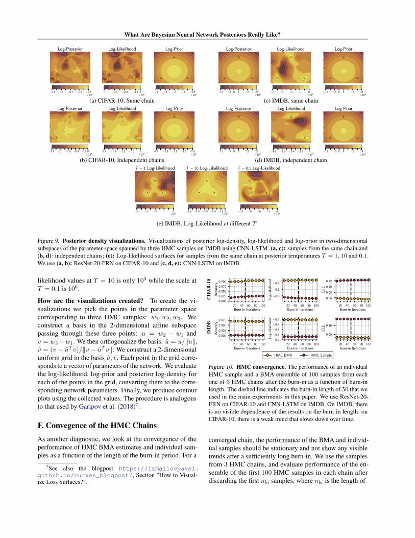
In Figure 9(a) we visualize the posterior log-density, log-likelihood and log-prior density of a ResNet-20-FRN onCIFAR-10. For the visualization, we use the subspace Sdefined by the parameter vectors w1, w51 and w101, thesamples produced by HMC at iterations 1, 51 and 101 af-ter burn-in respectively. We observe that HMC is able tonavigate complex geometry: the samples fall in three seem-ingly isolated modes in our two-dimensional cross-sectionof the posterior. In other words, HMC samples from a singlechain are not restricted to any specific convex Gaussian-likemode, and instead explore a region of high posterior densityof a complex shape in the parameter space. We note thatpopular approximate inference procedures, such as varia-tional methods, and Laplace approximations, are typicallyconstrained to unimodal Gaussian approximations to theposterior, which we indeed expect to miss a large space ofcompelling solutions in the posterior.

In Figure 9(b) we provide a visualization for the samplesproduced by 3 different HMC chains at iteration 51 afterburn-in. Comparing the visualizations for samples fromthe same chain and samples from independent chains inFigure 9, we see that the shapes of the posterior surfacesare different, with the latter appearing more regular andsymmetric. The qualitative differences between (a) and (b)suggest that while each HMC chain is able to navigate theposterior geometry the chains do not mix perfectly in theweight space, confirming our results in Section 5.1.

In Figure 9(c, d) we provide analogous visualizations for theCNN-LSTM architecture on IMDB. On IMDB, the posteriorlog-density is dominated by the prior, and the correspond-ing panels (c, d) are virtually indistinguishable in Figure 9.For the CNN-LSTM on IMDB the number of parametersis much larger than the number of data points, and hencethe scale of the prior density values is much larger than thescale of the likelihood. Note that the likelihood still affectsthe posterior typical set, and the HMC samples land in themodes of the likelihood in the visualization. In contrast,on ResNet-20, the number of parameters is smaller and thenumber of data points is larger, so the posterior is domi-nated by the likelihood in Figure 9 (a, b). On IMDB, thevisualizations for samples from a single chain and for sam-ples from three independent chains are qualitatively quitesimilar, hinting at better parameter-space mixing comparedto CIFAR-10 (see Section 5.1).

In Figure 9 (e), we visualize the likelihood cross-sectionsusing our runs with varying posterior temperature on IMDB.The visualizations show that, as expected, low temperatureleads to a sharp likelihood, while the high-temperature like-lihood appear soft. In particular, the scale of the lowest


×106

Log-Posterior

−1.3 −1 −0.7 −0.4 −0.4×106

Log-Likelihood

−1. −0.7 −0.4 −0.1 0×105

Log-Prior

−5 −3 −2 −1 −0.5

(a) CIFAR-10, Same chain

×106

Log-Posterior

-2.7 −2.1 −1.5 −0.9 -0.3 0×106

Log-Likelihood

-2.4 −1.8 −1.2 −0.6 0×105

Log-Prior

-4.5 −3.5 −2.5 −1.5 -0.5

(b) CIFAR-10, Independent chains

×105

Log-Posterior

−15 −5 0 5 15 25×105

Log-Likelihood

−4 −3 −2 −1 0×105

Log-Prior

−15 −5 0 5 15 25

(c) IMDB, same chain

×105

Log-Posterior

−15 −5 0 5 15 25×105

Log-Likelihood

−4.8 −3.6 −2.4 −1.2 0×105

Log-Prior

−15 −5 0 5 15 25

(d) IMDB, independent chain

×104

T = 1 Log-Likelihood

−4 −3 −2 1 0×103

T = 10 Log-Likelihood

−5.5 −4.5 −3.5 −2.5 -1.5 -1×105

T = 0.1 Log-Likelihood

−12 −9 −6 −3 0

(e) IMDB, Log-Likelihood at different T

Figure 9. Posterior density visualizations. Visualizations of posterior log-density, log-likelihood and log-prior in two-dimensionalsubspaces of the parameter space spanned by three HMC samples on IMDB using CNN-LSTM. (a, c): samples from the same chain and(b, d): independent chains; (e): Log-likelihood surfaces for samples from the same chain at posterior temperatures T = 1, 10 and 0.1.We use (a, b): ResNet-20-FRN on CIFAR-10 and (c, d, e): CNN-LSTM on IMDB.

likelihood values at T = 10 is only 103 while the scale atT = 0.1 is 106.

How are the visualizations created? To create the vi-sualizations we pick the points in the parameter spacecorresponding to three HMC samples: w1, w2, w3. Weconstruct a basis in the 2-dimensional affine subspacepassing through these three points: u = w2 − w1 andv = w3−w1. We then orthogonalize the basis: u = u/‖u‖,v = (v − uT v)/‖v − uT v‖. We construct a 2-dimensionaluniform grid in the basis u, v. Each point in the grid corre-sponds to a vector of parameters of the network. We evaluatethe log-likelihood, log-prior and posterior log-density foreach of the points in the grid, converting them to the corre-sponding network parameters. Finally, we produce contourplots using the collected values. The procedure is analogousto that used by Garipov et al. (2018)7.

F. Convegence of the HMC ChainsAs another diagnostic, we look at the convergence of theperformance of HMC BMA estimates and individual sam-ples as a function of the length of the burn-in period. For a

7See also the blogpost https://izmailovpavel.github.io/curves_blogpost/, Section ”How to Visual-ize Loss Surfaces?”.

CIF

AR

-10

20 40 60 80 100Burn-in Iterations

0.800

0.825

0.850

0.875

0.900

Acc

urac

y


−0.8

−0.6

−0.4

Log

-Lik

elih

ood


0.06

0.08

0.10

0.12

EC

E

IMD

B


0.800

0.825

0.850

0.875

Acc

urac

y


−0.7

−0.6

−0.5

−0.4

−0.3

Log

-Lik

elih

ood


0.05

0.10E

CE

HMC BMA HMC Sample

Figure 10. HMC convergence. The performance of an individualHMC sample and a BMA ensemble of 100 samples from eachone of 3 HMC chains after the burn-in as a function of burn-inlength. The dashed line indicates the burn-in length of 50 that weused in the main experiments in this paper. We use ResNet-20-FRN on CIFAR-10 and CNN-LSTM on IMDB. On IMDB, thereis no visible dependence of the results on the burn-in length; onCIFAR-10, there is a weak trend that slows down over time.

converged chain, the performance of the BMA and individ-ual samples should be stationary and not show any visibletrends after a sufficiently long burn-in. We use the samplesfrom 3 HMC chains, and evaluate performance of the en-semble of the first 100 HMC samples in each chain afterdiscarding the first nbi samples, where nbi is the length of

https://izmailovpavel.github.io/curves_blogpost/

https://izmailovpavel.github.io/curves_blogpost/


METHOD CIFAR-10 CIFAR-100 IMDB

ACC LOG-LIK ECE ACC LOG-LIK ECE ACC LOG-LIK ECE

SGD 83.4 -0.800 0.119 47.8 -2.364 0.193 82.9 -0.755 0.136HMC 90.7 -0.307 0.059 69.3 -1.134 0.134 86.8 -0.308 0.033SGLD 89.3 -0.341 0.052 63.6 -1.404 0.148 86.1 -0.314 0.007

DE 89.2 -0.331 0.028 65.6 -1.385 0.170 85.8 -0.358 0.042SGLD (5 CHAINS) 90.1 -0.327 0.066 66.9 -1.342 0.195 86.6 -0.306 0.006

MFVI 86.5 -0.409 0.019 54.9 -1.749 0.032 85.4 -0.341 0.038

Table 6. Detailed results on CIFAR and IMDB. Accuracy, log-likelihood and expected calibration error for Hamiltonian Monte Carlo(HMC), stochastic gradient Langevin dynamics (SGLD) with 1 and 5 chains, mean field variational inference (MFVI), stochastic gradientdescent (SGD), and deep ensembles. We use ResNet-20-FRN on CIFAR datasets, and CNN-LSTM on IMDB. Bayesian neural networksvia HMC outperform all baselines on all datasets in terms of accuracy and log-likelihood; on IMDB the performance of 5-chain SGLD issimilar. All methods perform similarly well on ECE, except for SGD which is consistently poorly calibrated.

1 2 3 4 5

Intensity

0.84

0.86

0.88

0.90

Acc

urac

y

Brightness

1 2 3 4 5

Intensity

−0.5

−0.4

−0.3

Log

-Lik

elih

oo

d

Brightness

1 2 3 4 5

Intensity

0.04

0.06

EC

E

Brightness

1 2 3 4 5

Intensity

0.5

0.6

0.7

0.8

0.9

Acc

urac

y

Contrast

1 2 3 4 5

Intensity

−1.5

−1.0

−0.5

Log

-Lik

elih

oo

d

Contrast

1 2 3 4 5

Intensity

0.02

0.04

0.06

0.08

EC

E

Contrast

1 2 3 4 5

Intensity

0.7

0.8

0.9

Acc

urac

y

Defocus Blur

1 2 3 4 5

Intensity

−1.0

−0.8

−0.6

−0.4

Log

-Lik

elih

oo

d

Defocus Blur

1 2 3 4 5

Intensity

0.02

0.04

0.06

0.08

EC

E

Defocus Blur

1 2 3 4 5

Intensity

0.75

0.80

0.85

Acc

urac

y

Elastic

1 2 3 4 5

Intensity

−0.8

−0.6

Log

-Lik

elih

oo

d

Elastic

1 2 3 4 5

Intensity

0.04

0.06

0.08

EC

E

Elastic

1 2 3 4 5

Intensity

0.7

0.8

0.9

Acc

urac

y

Fog

1 2 3 4 5

Intensity

−1.0

−0.8

−0.6

−0.4

Log

-Lik

elih

oo

d

Fog

1 2 3 4 5

Intensity

0.02

0.04

0.06

0.08

EC

E

Fog

1 2 3 4 5

Intensity

0.65

0.70

0.75

0.80

0.85

Acc

urac

y

Frost

1 2 3 4 5

Intensity

−1.2

−1.0

−0.8

−0.6

−0.4

Log

-Lik

elih

oo

d

Frost

1 2 3 4 5

Intensity

0.02

0.04

0.06

0.08

0.10

EC

E

Frost

1 2 3 4 5

Intensity

0.50

0.55

0.60

0.65

Acc

urac

y

Frosted Glass Blur

1 2 3 4 5

Intensity

−2.00

−1.75

−1.50

−1.25

−1.00

Log

-Lik

elih

oo

d

Frosted Glass Blur

1 2 3 4 5

Intensity

0.05

0.10

0.15

0.20

EC

E

Frosted Glass Blur

1 2 3 4 5

Intensity

0.5

0.6

0.7

0.8

0.9

Acc

urac

y

Gaussian Blur

1 2 3 4 5

Intensity

−1.5

−1.0

−0.5

Log

-Lik

elih

oo

d

Gaussian Blur

1 2 3 4 5

Intensity

0.05

0.10

EC

E

Gaussian Blur

1 2 3 4 5

Intensity

0.4

0.6

0.8

Acc

urac

y

Gaussian Noise

1 2 3 4 5

Intensity

−2.0

−1.5

−1.0

−0.5

Log

-Lik

elih

oo

d

Gaussian Noise

1 2 3 4 5

Intensity

0.0

0.1

0.2

0.3

EC

E

Gaussian Noise

1 2 3 4 5

Intensity

0.4

0.6

0.8

Acc

urac

y

Impulse Noise

1 2 3 4 5

Intensity

−2.0

−1.5

−1.0

−0.5

Log

-Lik

elih

oo

d

Impulse Noise

1 2 3 4 5

Intensity

0.1

0.2

EC

E

Impulse Noise

1 2 3 4 5

Intensity

0.5

0.6

0.7

0.8

0.9

Acc

urac

y

Pixelate

1 2 3 4 5

Intensity

−2.0

−1.5

−1.0

−0.5

Log

-Lik

elih

oo

d

Pixelate

1 2 3 4 5

Intensity

0.05

0.10

0.15

0.20

EC

E

Pixelate

1 2 3 4 5

Intensity

0.82

0.84

0.86

0.88

0.90

Acc

urac

y

Saturate

1 2 3 4 5

Intensity

−0.6

−0.5

−0.4L

og-L

ikel

iho

od

Saturate

1 2 3 4 5

Intensity

0.04

0.06

0.08

EC

E

Saturate

1 2 3 4 5

Intensity

0.4

0.6

0.8

Acc

urac

y

Shot Noise

1 2 3 4 5

Intensity

−2.0

−1.5

−1.0

−0.5

Log

-Lik

elih

oo

d

Shot Noise

1 2 3 4 5

Intensity

0.0

0.1

0.2

EC

E

Shot Noise

1 2 3 4 5

Intensity

0.75

0.80

0.85

Acc

urac

y

Spatter

1 2 3 4 5

Intensity

−0.8

−0.6

−0.4

Log

-Lik

elih

oo

d

Spatter

1 2 3 4 5

Intensity

0.04

0.06

0.08

0.10

EC

E

Spatter

1 2 3 4 5

Intensity

0.4

0.6

0.8

Acc

urac

y

Speckle Noise

1 2 3 4 5

Intensity

−1.5

−1.0

−0.5

Log

-Lik

elih

oo

d

Speckle Noise

1 2 3 4 5

Intensity

0.05

0.10

0.15

0.20

EC

E

Speckle Noise

1 2 3 4 5

Intensity

0.7

0.8

Acc

urac

y

Zoom Blur

1 2 3 4 5

Intensity

−1.0

−0.8

−0.6

−0.4

Log

-Lik

elih

oo

d

Zoom Blur

1 2 3 4 5

Intensity

0.02

0.04

0.06

0.08

EC

E

Zoom Blur

HMC SGD Deep Ens SGLD SGHMC-CLR-Prec

Figure 11. Performance under corruption. We show accuracy, log-likelihood and ECE of HMC, SGD, Deep Ensembles, SGLD andSGHMC-CLR-Prec for all 16 CIFAR-10-C corruptions as a function of corruption intensity. HMC shows poor accuracy on most of thecorruptions with a few exceptions. SGLD provides the best robustness on average.


the burn-in. Additionally, we evaluate the performance ofthe individual HMC samples after nbi iterations in each ofthe chains.

We report the results for ResNet-20-FRN on CIFAR-10 andCNN-LSTM on IMDB in Figure 10. On IMDB, there is novisible trend in performance, so a burn-in of just 10 HMCiterations should be sufficient. On CIFAR-10, we observea slowly rising trend that saturates at about 50 iterations,indicating that a longer burn-in period is needed comparedto IMDB. We therefore use a burn-in period of 50 HMCiterations on both CIFAR and IMDB for the remainder ofthe paper.

Is HMC Converging? In general, it is not possible toensure that an MCMC method has converged to samplingfrom the true posterior distribution: theoretically, there mayalways remain regions of the posterior that cannot be dis-covered by the method but that contain most of the posteriormass. To maximize the performance of HMC, we choosethe hyper-parameters that are the most likely to provide con-vergence: long trajectory lengths, and multiple long chains.In Section 5, we study the convergence of HMC using theavailable convergence diagnostics. We find that while HMCdoes not mix perfectly in weight space, in the space ofpredictions we cannot find evidence of non-mixing.

G. Detailed Results on CIFAR and IMDBIn Table 6 we report the accuracy, log-likelihood and ex-pected calibration error for each of the methods we consideron CIFAR and IMDB datasets. BNNs via HMC provide thebest performance on all datasets in terms of accuracy andlog-likelihood (with 5-chain SGLD achieving competitiveresults on IMDB), and all methods except SGD show goodcalibration in terms of ECE.

H. BNNs are not Robust to Domain ShiftIn Section 6.2, Figure 4 we have seen that surprisinglyBNNs via HMC underperform significantly on corrupteddata from CIFAR-10-C compared to SGLD, deep ensemblesand even MFVI and SGD. We provide detailed results in Fig-ure 11. HMC shows surprisingly poor robustness in termsof accuracy and log-likelihood across the corruptions. TheECE results are mixed. In most cases, the HMC ensembleof 720 models loses to a single SGD solution!

The poor performance of HMC on OOD data is surprising.Bayesian methods average the predictions over multiplemodels for the data, and faithfully represent uncertainty.Hence, Bayesian deep learning methods are expected to berobust to noise in the data, and are often explicitly evaluatedon CIFAR-10-C (e.g. Wilson & Izmailov, 2020; Dusenberryet al., 2020). Our results suggest that the improvements

0 2 4 6 8 10Gaussian Noise Scale

0.2

0.4

0.6

0.8

1.0

Acc

urac

y

SGD

HMC

Sample

HMC T = 10−3

Sample T = 10−3

Figure 12. Robustness on MNIST. Performance of SGD, BMAensembles and individual samples constructed by HMC at temper-atures T = 1 and T = 10−3 on the MNIST test set corrupted byGaussian noise. We use a fully-connected network. Temperature 1HMC shows very poor robustness, while lowering the temperatureallows us to close the gap to SGD.

achieved by Bayesian methods on corrupted data may be asign of poor posterior approximation.

To further understand the robustness results, we reproducethe same effect on a small fully-connected network withtwo hidden layers of width 256 on MNIST. We run HMC attemperatures T = 1 and T = 10−3 and SGD and report theresults for both the BMA ensembles and individual samplesin Figure 12. For all methods, we train the models on theoriginal MNIST training set, and evaluate on the test setwith random Gaussian noise N (0, σ2I) of varying scale σ.We report the test accuracy as a function of σ. We find thatwhile the performance on the original test set is very closefor all methods, the accuracy of HMC at T = 1 drops muchquicker compared to that of SGD as we increase the noisescale.

Notably, the individual sample performance of T = 1 HMCis especially poor compared to SGD. For example, at noisescale σ = 3 the SGD accuracy is near 60% while the HMCsample only achieves around 20% accuracy!

HMC can be though of as sampling points at a certain sub-optimal level of the training loss, significantly lower thanthat of SGD solutions. As a result, HMC samples are indi-vidually inferior to SGD solutions. On the original test dataensembling the HMC samples leads to strong performancesignificantly outperforming SGD (see Section 6). However,as we apply noise to the test data, ensembling can no longerclose the gap to the SGD solutions. To provide evidencefor this explanation, we run evaluate HMC at a very lowtemperature T = 10−3, as low temperature posteriors con-centrate on high-performance solutions similar to the onesfound by SGD. We find that at this temperature, HMC per-forms comparably with SGD, closing the gap in robustnessWe have also experimented with varying the prior scale butwere unable to close the gap in robustness at temperatureT = 1.

We hypothesize that using a lower temperature with HMC


AUC-ROC

OOD DATASET HMC DEEP ENS ODIN MAHALANOBIS

CIFAR-100 0.857 0.853 0.858 0.882SVHN 0.8814 0.8529 0.967 0.991

Table 7. Out-of-distribution detection. We use a ResNet-20-FRN model trained on CIFAR-10 to detect out-of-distribution data comingfrom SVHN or CIFAR-100. We report the results for HMC, deep ensembles and specialized ODIN (Liang et al., 2017) and Mahalanobis(Lee et al., 2018) methods. We report the AUC-ROC score (higher is better) evaluating the ability of each method to distinguishbetween in-distribution and OOD data. The predictive uncertainty from Bayesian neural networks allows us to detect OOD inputs: HMCoutpeforms deep ensembles on both datasets. Moreover, HMC is competitive with ODIN on the harder near-OOD task of detectingCIFAR-100 images, but underperforms on the easier far-OOD task of detecting SVHN images.

ACC, T = 1 ACC, T = 0.1 CE, T = 1 CE, T = 0.1

BN + AUG 87.46 91.12 0.376 0.2818FRN + AUG 85.47 89.63 0.4337 0.317BN + NO AUG 86.93 85.20 0.4006 0.4793FRN + NO AUG 84.27 80.84 0.4708 0.5739

Table 8. Role of data augmentation in the cold posterior effect. Results of a single chain ensemble constructed with the SGHMC-CLR-Prec sampler of Wenzel et al. (2020) at temperatures T = 1 and T = 0.1 for different combinations of batch normalization (BN) orfilter response normalization (FRN) and data augmentation (Aug). We use the ResNet-20 architecture on CIFAR-10. Regardless of thenormalization technique, the cold posteriors effect is present when data augmentation is used, and not present otherwise.

would also significantly improve robustness on CIFAR-10-C. Verifying this hypothesis, and generally understandingthe robustness of BNNs further is an exciting direction offuture work8.

I. Out-of-Distribution DetectionBayesian deep learning methods are often evaluated on out-of-distribution detection. In Table 7 we report the perfor-mance of an HMC-based Bayesian neural network on out-of-distribution (OOD) detection. To detect OOD data, weuse the level of predicted confidence (value of the softmaxclass probability for the predicted class) from the HMCensemble, measuring the area under the receiving operatorcharacteristic curve (AUC-ROC). We train the methods onCIFAR-10 and use CIFAR-100 and SVHN as OOD datasources.

We find that BNNs perform competitively with the special-ized ODIN method in the challenging near-OOD detectionsetting (i.e. when the OOD data distribution is similar to thetraining data) of CIFAR-100, while underperforming in theeasier far-OOD setting on SVHN relative to the baselines(Liang et al., 2017; Lee et al., 2018).

8In a follow-up work, Izmailov et al. (2021) provide a de-tailed explanation for why Bayesian neural networks can fail undercovariate shift. In particular, they find that tempering does notgenerally improve robustness, and propose alternative resolutions.

J. Further Discussion of Cold PosteriorsIn Section 7 we have seen that the cold posteriors are notneeded to achieve strong performance with BNNs. We haveeven shown that cold (as well as warm) posteriors mayhurt the performance. On the other hand, in Appendix Hwe have shown that lowering the temperature can improverobustness under the distribution shift, at least for a smallMLP on MNIST. Here, we discuss the potential reasons forwhy the cold posteriors effect was observed in Wenzel et al.(2020).

J.1. What Causes the Difference with Wenzel et al.(2020)?

There are several key differences between the experimentsin our study and Wenzel et al. (2020).

First of all, the predictive distributions of SGLD (a ver-sion of which was used in Wenzel et al. (2020)) are highlydependent on the hyper-parameters such as the batch sizeand learning rate, and are inherently biased: SGLD with anon-vanishing step size samples from a perturbed version ofthe posterior, both because it omits a Metropolis-Hastingsaccept-reject step and because its updates include minibatchnoise. Both of these perturbations should tend to make theentropy of SGLD’s stationary distribution increase with itsstep size; we might expect this to translate to approximationsto the BMA that are overdispersed.

Furthermore, Wenzel et al. (2020) show in Figure 6 thatwith a high batch size they achieve good performance at


Figure 13. HMC samples are (over)confident classifiers. Plots show the probability assigned by a series of HMC samples to the truelabel of a held-out CIFAR-10 image. In many cases these probabilities are overconfident (i.e., assign the right answer probability near 0),but there are always some samples that assign the true label high probability, so the Bayesian model average is both accurate and wellcalibrated. These samples were generated with a spherical Gaussian prior with variance 1

5.

T = 1 for the CNN-LSTM. Using the code provided by theautors9 with default hyper-parameters we achieved strongperformance at T = 1 for the CNN-LSTM (accuracy of0.855 and cross-entropy of 0.35, compared to 0.81 and 0.45reported in Figure 1 of Wenzel et al. (2020)); we were,however, able to reproduce the cold posteriors effect onCIFAR-10 using the same code.

On CIFAR-10, the main difference between our setup andthe configuration in Wenzel et al. (2020) is the use of batchnormalization and data augmentation. In the appendix Kand Figure 28 of Wenzel et al. (2020), the authors showthat if both the data augmentation and batch normalizationare turned off, we no longer observe the cold posteriorseffect. In Table 8 we confirm using the code provided bythe authors that in fact it is sufficient to turn off just the dataaugmentation to remove the cold posteriors effect. It is thuslikely that the results in Wenzel et al. (2020) are at leastpartly affected by the use of data augmentation.

K. Effect of Gaussian Prior ScaleWe use priors of the form N (0, α2I) and vary the priorvariance α2. For all cases, we use a single HMC chainproducing 40 samples. These are much shorter chains thanthe ones we used in Section 6, so the results are not asgood; the purpose of this section is to explore the relativeperformance of BNNs under different priors.

We report the results for the CIFAR-10 and IMDB datasets

9https://github.com/google-research/google-research/tree/master/cold_posterior_bnn

CIF

AR

-10

140

120

110

15

1

Prior Variance α2

0.84

0.86

0.88

Acc

urac

y

140

120

110

15

1

Prior Variance α2

−0.8

−0.6

−0.4

Log

-Lik

elih

ood

140

120

110

15

1

Prior Variance α2

0.025

0.050

0.075

0.100

0.125

EC

E

IMD

B

1160

180

140

120

1

Prior Variance α2

0.84

0.86

Acc

urac

y

1160

180

140

120

1

Prior Variance α2

−0.8

−0.6

−0.4L

og-L

ikel

ihoo

d

1160

180

140

120

1

Prior Variance α2

0.05

0.10

EC

E

Figure 14. Effect of prior variance. The effect of prior varianceon BNN performance. In each panel, the dashed line shows theperformance of the SGD model from Section 6. While low priorvariance may lead to over-regularization and hurt performance, allthe considered prior scales lead to better results than the perfor-mance of an SGD-trained neural network of the same architecture.

in Figure 14. When the prior variance is too small, theregularization is too strong, hindering the performance. Set-ting the prior variance too large does not seem to hurt theperformance as much. On both problems, the performanceis fairly robust: a wide window of prior variances lead tostrong performance. In particular, for all considered priorscales, the results are better than those of SGD training.

Why are BNNs so robust to the prior scale? One pos-sible explanation for the relatively flat curves in Figure 14is that large prior variances imply a strong prior belief thatthe “true” classifier (i.e., the model that would be learnedgiven infinite data) should make high-confidence predictions.Since the model is powerful enough to achieve any desiredtraining accuracy, the likelihood does not overrule this prior

https://github.com/google-research/google-research/tree/master/cold_posterior_bnn




belief, and so the posterior assigns most of its mass to veryconfident classifiers. Past a certain point, increasing theprior variance on the weights may have no effect on the clas-sifiers’ already saturated probabilities. Consequently, nearlyevery member of the BMA may be highly overconfident.But the ensemble does not have to be overconfident—a mix-ture of overconfident experts can still make well-calibratedpredictions. Figure 13 provides some qualitative evidencefor this explanation; for some CIFAR-10 test set images,the HMC chain oscillates between assigning the true labelprobabilities near 1 and probabilities near 0.

L. Predictive Entropy and Calibration Curvesfor HMC and Scalable BDL Methods

In Figure 15 we visualize the distribution of predictive en-tropies and the calibration curves for HMC, SGD, deep en-sembles, MFVI, SGLD and SGHMC-CLR-Prec on CIFAR-10 using ResNet-20-FRN.

1k

3k

5kHMC SGLD SGHMC

CLR-Prec

0 1 2

1k

3k

5kSGD

0 1 2

MFVI

0 1 2

Deep Ens

0.4 0.6 0.8 1.0

Confidence

−0.05

0.00

0.05

0.10

0.15

Acc

urac

y-

Con

fide

nce

HMC

SGLD

SGHMC-CLR-Prec

MFVI

SGD

Deep Ens

Figure 15. Distribution of predictive entropies (left) and calibra-tion curve (right) of posterior predictive distributions for HMC,SGD, deep ensembles, MFVI, SGLD and SGHMC-CLR-Prec forResNet20-FRN on CIFAR-10. On the left, for all methods, exceptHMC we plot a pair of histograms: for HMC and for the corre-sponding method. SGD, Deep ensembles and MFVI provide moreconfident predictions than HMC. SGMCMC methods appear tofit the predictive distribution of HMC better: SGLD is slightly un-derconfident relative to HMC while SGHMC-CLR-Prec is slightlyover-confident.

All methods except fot SGD make conservative predictions:their confidences tend to underestimate their accuracies (Fig-ure 15, right); SGD on the other hand is very over-confident(in agreement with the results in Guo et al., 2017). Deepensembles and MFVI provide the most calibrated predic-tions, while SGLD and SGHMC-CLR-Prec match the HMCentropy distribution and calibration curve closer.

Documents

What Are Bayesian Neural Network Posteriors Really Like?