Embed Size (px)
Citation preview
Original paperData preparation
Data processing and visualization
Westward shift of western North Pacifictropical cyclogenesis
Wu et al. (2015), Geophys. Res. Lett.doi:10.1002/2015GL063450
Jonathon S. Wright
21 March, 2017
Original paperData preparation
Data processing and visualization
Original paperIntroductionResultsDiscussion
Data preparationThe netCDF4 moduleThe datetime modulePre-processing
Data processing and visualizationMapping: the cartopy moduleLinear regression and correlationsMore contour plots and masked arrays

Original paperData preparation
Data processing and visualization
IntroductionResults
Motivation
I Tropical cyclones in Western North Pacific account for aboutone third of all TCs
I Changes in TC genesis location could affect billions of people
Previous studies indicate that TC genesis location may change
I Poleward movement of mean TC max intensity
I Large-scale changes in vertical wind shear and potentialintensity
I Changes in the distribution of mid-tropospheric RH
I More synoptic-scale disturbances in central Pacific
Original paperData preparation
Data processing and visualization
IntroductionResults
The tropical upper tropospheric trough
I Extends from 15◦N in the WNP to 35◦N in the ENP
I Apparent in 200 hPa wind field during boreal summer
I Strong vertical wind shear along the eastern flank limitseastward extension of TC activity in WNP
Data and methodology
I Tropical cyclone best track data: JTWC and ADT-HURSAT
I Reanalysis data: 20CR, NCEP-NCAR, ERA-Interim, JRA-25,MERRA, NCEP-DOE, CFSR
I Linear trends and correlations, with significance testing
Original paperData preparation
Data processing and visualization
IntroductionResults
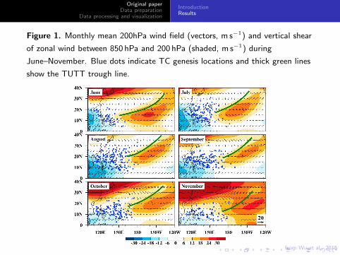
from Wu et al., 2015
Figure 1. Monthly mean 200hPa wind field (vectors, m s−1) and vertical shear
of zonal wind between 850 hPa and 200 hPa (shaded, m s−1) during
June–November. Blue dots indicate TC genesis locations and thick green lines
show the TUTT trough line.

Original paperData preparation
Data processing and visualization
IntroductionResults
from Wu et al., 2015
Figure 2. Time series of (a) annual mean TC genesis longitude (blue) from the
JTWC dataset and annual mean TUTT longitude (red), and (b) annual mean
TC longitude from the ADT-HURSAT data set with (blue) and without (red)
the ENSO effect.

Original paperData preparation
Data processing and visualization
IntroductionResults
from Wu et al., 2015
Figure 3. Annual means of (a) TC formation frequency in the western and
eastern portions of the WNP basin, and (b) the difference of the tropospheric
temperature (red, K) between the tropics and the subtropics and the vertical
shear of the zonal wind (m s−1) in the TUTT region.
Original paperData preparation
Data processing and visualization
IntroductionResults
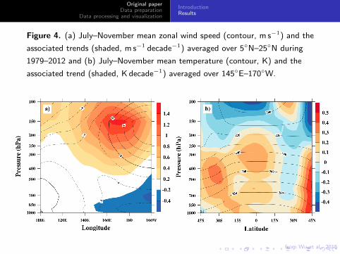
from Wu et al., 2015
Figure 4. (a) July–November mean zonal wind speed (contour, m s−1) and the
associated trends (shaded, m s−1 decade−1) averaged over 5◦N–25◦N during
1979–2012 and (b) July–November mean temperature (contour, K) and the
associated trend (shaded, K decade−1) averaged over 145◦E–170◦W.
Original paperData preparation
Data processing and visualization
The netCDF4 moduleThe datetime modulePre-processing
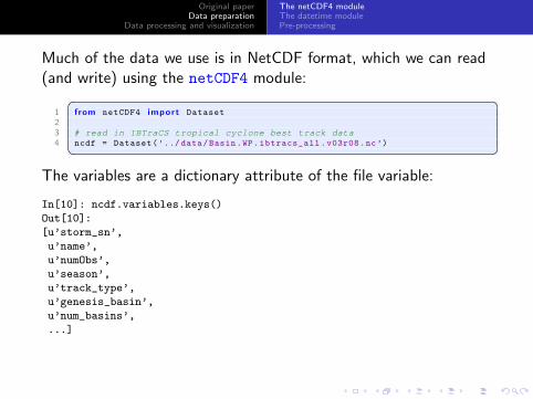
Much of the data we use is in NetCDF format, which we can read(and write) using the netCDF4 module:� �
1 from netCDF4 import Dataset
23 # read in IBTraCS tropical cyclone best track data4 ncdf = Dataset(’../ data/Basin.WP.ibtracs_all.v03r08.nc’)� �
The variables are a dictionary attribute of the file variable:
In[10]: ncdf.variables.keys()
Out[10]:
[u’storm_sn’,
u’name’,
u’numObs’,
u’season’,
u’track_type’,
u’genesis_basin’,
u’num_basins’,
...]
Original paperData preparation
Data processing and visualization
The netCDF4 moduleThe datetime modulePre-processing
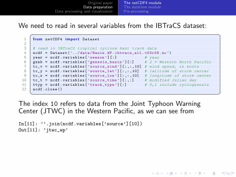
We need to read in several variables from the IBTraCS dataset:� �1 from netCDF4 import Dataset
23 # read in IBTraCS tropical cyclone best track data4 ncdf = Dataset(’../ data/Basin.WP.ibtracs_all.v03r08.nc’)
5 year = ncdf.variables[’season ’][:] # year6 genb = ncdf.variables[’genesis_basin ’][:] # 2 = Western North Pacific7 tc_v = ncdf.variables[’source_wind ’][:,:,10] # wind speed, in knots8 tc_y = ncdf.variables[’source_lat ’][:,:,10] # latitude of storm center9 tc_x = ncdf.variables[’source_lon ’][:,:,10] # longitude of storm center
10 tc_t = ncdf.variables[’source_time ’][:,:] # modified Julian day11 ttyp = ncdf.variables[’track_type ’][:] # 0,1 include cyclogenesis12 ncdf.close()� �
The index 10 refers to data from the Joint Typhoon WarningCenter (JTWC) in the Western Pacific, as we can see from
In[11]: ’’.join(ncdf.variables[’source’][10])
Out[11]: ’jtwc_wp’
Original paperData preparation
Data processing and visualization
The netCDF4 moduleThe datetime modulePre-processing
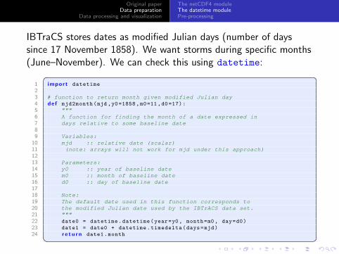
IBTraCS stores dates as modified Julian days (number of dayssince 17 November 1858). We want storms during specific months(June–November). We can check this using datetime:� �
1 import datetime
23 # function to return month given modified Julian day4 def mjd2month(mjd ,y0=1858,m0=11,d0=17):
5 """6 A function for finding the month of a date expressed in7 days relative to some baseline date89 Variables:
10 mjd :: relative date (scalar)11 (note: arrays will not work for mjd under this approach)1213 Parameters:14 y0 :: year of baseline date15 m0 :: month of baseline date16 d0 :: day of baseline date1718 Note:19 The default date used in this function corresponds to20 the modified Julian date used by the IBTrACS data set.21 """22 date0 = datetime.datetime(year=y0, month=m0 , day=d0)
23 date1 = date0 + datetime.timedelta(days=mjd)
24 r e t u r n date1.month� �
Original paperData preparation
Data processing and visualization
The netCDF4 moduleThe datetime modulePre-processing
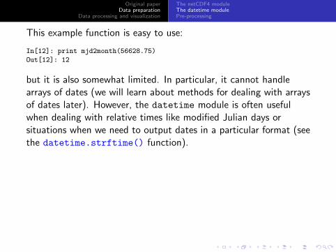
This example function is easy to use:
In[12]: print mjd2month(56628.75)
Out[12]: 12
but it is also somewhat limited. In particular, it cannot handlearrays of dates (we will learn about methods for dealing with arraysof dates later). However, the datetime module is often usefulwhen dealing with relative times like modified Julian days orsituations when we need to output dates in a particular format (seethe datetime.strftime() function).

Original paperData preparation
Data processing and visualization
The netCDF4 moduleThe datetime modulePre-processing
We then need to find the genesis locations, which in this case aredefined as the first time that the maximum windspeed exceeded 25knots (∼13 m s−1):� �
1 import numpy as np
23 # loop through storms and find genesis locations4 cgx = []; cgy = []; cgm = []
5 # start with all tracks that include cyclogenesis in the WP6 sdx = np.where ((( ttyp == 0) | (ttyp == 1)) & (genb == 2))[0]
7 # note that loop is over indices, not over a range!8 f o r ss i n sdx:
9 #−− check to see if the wind ever exceeds 25 knots10 i f np.any(tc_v[ss ,:] >= 25):
11 cg = np.where(tc_v[ss ,:] >= 25) [0][0]
12 #−−−−−− append lat/lon/month of cyclogenesis13 cgy.append(tc_y[ss,cg])
14 cgx.append(tc_x[ss,cg])
15 cgm.append(mjd2month(tc_t[ss,cg]))
16 # convert to arrays17 cgy = np.array(cgy)
18 cgx = np.array(cgx)
19 cgm = np.array(cgm)
20 # longitude in IBTraCS is (−180,180); convert to (0,360)21 cgx[cgx < 0] += 360� �

Original paperData preparation
Data processing and visualization
The netCDF4 moduleThe datetime modulePre-processing
We also need some reanalysis data for the winds and temperatures.Here, we will use the JRA-55 reanalysis, which was not used in theoriginal paper. The data files are quite large, and it is thereforeconvenient to preprocess the files to make them manageable. Todo this, I use the Climate Data Operators (CDO) utilitiesdeveloped at the Max-Planck Institut fur Meteorologie. First, Iselect the temperature and wind data for June through Novemberusing the selmon (select month) command:
cdo selmon,6,7,8,9,10,11 jra55nl_tmp_monthly_1958-2015.nc4 tmp_jjason.nc4
cdo selmon,6,7,8,9,10,11 jra55nl_ugrd_monthly_1958-2015.nc4 uwd_jjason.nc4
cdo selmon,6,7,8,9,10,11 jra55nl_vgrd_monthly_1958-2015.nc4 vwd_jjason.nc4
CDO can be installed by downloading and installing the sourcefrom the project website, but on Mac OSX it is easier to useMacPorts or Homebrew. CDO has excellent documentation.
Original paperData preparation
Data processing and visualization
The netCDF4 moduleThe datetime modulePre-processing
To produce a JRA-55 version of Fig. 1 from the paper, we need todo a bit more preprocessing using CDO. Specifically, we need tocalculate monthly climatologies of zonal and meridional winds over1958–2015 using the ymonmean command, which calculatesmonthly means spanning multiple years (i.e., an annual cycle):
cdo ymonmean uwd_jjason.nc4 uwd_jjason_mm.nc4
cdo ymonmean vwd_jjason.nc4 vwd_jjason_mm.nc4
and then select the 200 and 850 hPa levels, removing the rest ofthe vertical profile (recall that we only need 850 hPa zonal wind tocalculate vertical shear, and do not need 850 hPa meridional wind):
cdo sellevel,85000,20000 uwd_jjason_mm.nc4 fig1_uwd.nc4
cdo sellevel,20000 vwd_jjason_mm.nc4 fig1_vwd.nc4

Original paperData preparation
Data processing and visualization
The netCDF4 moduleThe datetime modulePre-processing
We can then read in the data and calculate the zonal wind shear:� �1 from netCDF4 import Dataset
23 # read in JRA−55 wind data4 ncdf = Dataset(ddir+’fig1_uwd.nc4’)
5 jlon = ncdf.variables[’lon’][:]
6 jlat = ncdf.variables[’lat’][:]
7 u850 = ncdf.variables[’ugrd’][:,0,:,:]
8 u200 = ncdf.variables[’ugrd’][:,1,:,:]
9 ncdf.close()
10 ncdf = Dataset(ddir+’fig1_vwd.nc4’)
11 v200 = ncdf.variables[’vgrd’][:,0,:,:]
12 ncdf.close()
13 # calculate vertical wind shear14 ushr = u850 -u200� �
Original paperData preparation
Data processing and visualization
Mapping: the cartopy moduleLinear regression and correlationsMore contour plots and masked arrays
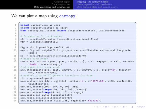
We can plot a map using cartopy:� �1 import cartopy.crs as ccrs
2 import cartopy.feature as cfeat
3 from cartopy.mpl.ticker import LongitudeFormatter , LatitudeFormatter
45 # formatting for tick marks6 xfr = LongitudeFormatter(zero_direction_label=True)
7 yfr = LatitudeFormatter ()
89 fig = plt.figure(figsize =(13, 4))
10 axs = fig.add_subplot (111, projection=ccrs.PlateCarree(central_longitude
=180))
11 prj = ccrs.PlateCarree(central_longitude =0)
12 # zonal wind shear13 cs0 = axs.contourf(jlon , jlat , ushr[0,:,:], clv , cmap=plt.cm.PuOr , extend=
’both’, transform=prj)
14 # streamplot to show winds15 axs.streamplot(jlon , jlat , u200[0,:,:], v200[0,:,:], color=’k’, density=
dns , transform=prj)
16 # scatter plot of TC genesis locations for June17 idx = np.where(cgm ==6)
18 axs.scatter(cgx[idx], cgy[idx], marker=’o’, c=’#377 eb8’, s=50, zorder =10,
transform=prj)
19 axs.set_extent ([100, 240, 0, 40], prj)
20 axs.set_xticks( range (100, 241, 20), crs=prj)
21 axs.set_yticks( range (0, 41, 10), crs=prj)
22 axs.xaxis.set_major_formatter(xfr)
23 axs.yaxis.set_major_formatter(yfr)
24 axs.add_feature(cfeat.COASTLINE , edgecolor=’#333333 ’)� �
Original paperData preparation
Data processing and visualization
Mapping: the cartopy moduleLinear regression and correlationsMore contour plots and masked arrays
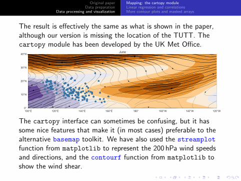
The result is effectively the same as what is shown in the paper,although our version is missing the location of the TUTT. Thecartopy module has been developed by the UK Met Office.
100°E 120°E 140°E 160°E 180° 160°W 140°W 120°W0°
10°N
20°N
30°N
40°NJune
The cartopy interface can sometimes be confusing, but it hassome nice features that make it (in most cases) preferable to thealternative basemap toolkit. We have also used the streamplot
function from matplotlib to represent the 200 hPa wind speedsand directions, and the contourf function from matplotlib toshow the wind shear.

Original paperData preparation
Data processing and visualization
Mapping: the cartopy moduleLinear regression and correlationsMore contour plots and masked arrays
Adding the location of the TUTT is more challenging, as the paperdoes not describe this procedure clearly. The authors mention thatthe TUTT is defined as the location where easterly windstransition to westerly; here, I have extrapolated from the idea thatthe transition from easterly to westerly indicates mass divergenceto define the TUTT location at each latitude as the longitude ofthe maximum (positive) zonal gradient in zonal wind.� �
1 import numpy as np
2 # for smoothing the visualization of the TUTT3 from statsmodels.nonparametric.smoothers_lowess import lowess
45 # TUTT6 ttt = np.empty (20)
7 f o r yy i n range (45 ,65):8 dux = np.gradient(np.squeeze(u200[5,yy,xdx]))
9 ttt[yy -45] = jlon[xdx[dux.argmax ()]]
10 tut = lowess(ttt , jlat [45:65] , frac =0.75 , return_sorted=False)
11 axs.plot(tut , jlat [45:65] , color=’#999999 ’, linewidth=3, transform=prj)� �I have also used a local regression (lowess) filter from thestatsmodels module to smooth the curve.
Original paperData preparation
Data processing and visualization
Mapping: the cartopy moduleLinear regression and correlationsMore contour plots and masked arrays
100°E 120°E 140°E 160°E 180° 160°W 140°W 120°W0°
10°N
20°N
30°N
40°NJune
100°E 120°E 140°E 160°E 180° 160°W 140°W 120°W0°
10°N
20°N
30°N
40°NJuly
100°E 120°E 140°E 160°E 180° 160°W 140°W 120°W0°
10°N
20°N
30°N
40°NAugust
100°E 120°E 140°E 160°E 180° 160°W 140°W 120°W0°
10°N
20°N
30°N
40°NSeptember
100°E 120°E 140°E 160°E 180° 160°W 140°W 120°W0°
10°N
20°N
30°N
40°NOctober
100°E 120°E 140°E 160°E 180° 160°W 140°W 120°W0°
10°N
20°N
30°N
40°NNovember

Original paperData preparation
Data processing and visualization
Mapping: the cartopy moduleLinear regression and correlationsMore contour plots and masked arrays
We need to do a bit more data processing to get the meanlongitude of cyclogenesis and the location of the TUTT between5◦N and 25◦N for each year:� �
1 # get mean longitude of cyclogenesis for each year2 yrs = np.arange (1958 ,2015)
3 mln = np.empty(yrs.shape)
4 f o r ii i n range ( l e n (yrs)):5 idx = np.where ((cgt == yrs[ii]) & (cgm >= 6) & (cgm <= 11))[0]
6 i f idx.any():7 mln[ii] = cgx[idx].mean()
89 # get location of TUTT (transition from easterlies to westerlies)
10 xdx = np.where((jlon >= 120) & (jlon <= 240))[0]
11 tutt = np.empty(yrs.shape)
12 f o r ii i n range ( l e n (yrs)):13 u = u200[ii,xdx]
14 x = jlon[xdx]
15 tutt[ii] = x[np.where(u > 0) [0][0]]� �

Original paperData preparation
Data processing and visualization
Mapping: the cartopy moduleLinear regression and correlationsMore contour plots and masked arrays
Once we have these variables, we have multiple options for trendanalysis. For example, we could use the scipy.stats module towork directly with the numpy arrays:� �
1 # linear regressions2 from scipy import stats
34 # linear regression over full time series5 a0,b0,r0 ,p0,s0 = stats.linregress(yrs ,mln)
6 #linear regression from 1979−20137 a1,b1,r1 ,p1,s1 = stats.linregress(yrs[21:],mln [21:])
89 # linear regression over full time series
10 a2,b2,r2 ,p2,s2 = stats.linregress(yrs ,tutt)
11 #linear regression from 1979−201312 a3,b3,r3 ,p3,s3 = stats.linregress(yrs[21:], tutt [21:])
1314 # linear correlation15 r,p = stats.pearsonr(mln ,tutt)� �stats.linregress returns the slope, intercept, correlationcoefficient R, 2-tailed p-value (that the slope is non-zero), and thestandard error of the slope estimate; stats.pearsonr returns thePearson correlation coefficient and the associated 2-tailed p-value.

Original paperData preparation
Data processing and visualization
Mapping: the cartopy moduleLinear regression and correlationsMore contour plots and masked arrays
A convenient alternative in many cases is to construct a pandas
DataFrame and use seaborn.regplot(), especially if we onlyneed to see the trend:� �
1 # −∗− coding: utf−8 −∗−2 import pandas as pd
3 import matplotlib.pyplot as plt
4 import seaborn as sns
56 # plot parameters7 sns.set_style(’darkgrid ’)
89 # make a pandas dataframe
10 df = pd.DataFrame ({’jtwc’:mln , ’tutt’:tutt}, index=yrs)
1112 # plot time series of mean longitude of cyclogenesis, with trends13 fig = plt.figure(figsize =(12 ,6))
14 axa = fig.add_subplot (211)
15 axa.plot(df.index , df[’jtwc’], ’-’, color=’#377 eb8’)
16 sns.regplot(df.index , df[’jtwc’], color=’#377 eb8’, ax=axa , truncate=True)
17 sns.regplot(df.ix [1979:]. index , df.ix [1979:][ ’jtwc’], color=’#377 eb8’,
18 line_kws ={’linestyle ’:’--’}, truncate=True , ci=None , ax=axa)
19 axa.set_xlabel(’’)
20 axa.set_xlim (1955 ,2015)
21 axa.set_xticks( range (1960, 2011, 10))
22 axa.set_ylabel(u’TC mean genesis longitude [\ u00b0E]’, color=’#377 eb8’)
23 axa.set_ylim (125 ,150)
24 axa.set_yticks( range (125 ,151 ,5))25 axa.set_yticklabels( range (125 ,151 ,5), color=’#377 eb8’)� �

Original paperData preparation
Data processing and visualization
Mapping: the cartopy moduleLinear regression and correlationsMore contour plots and masked arrays
� �1 sns.regplot(df.index , df[’jtwc’], color=’#377 eb8’, ax=axa , truncate=True)
2 sns.regplot(df.ix [1979:]. index , df.ix [1979:][ ’jtwc’], color=’#377 eb8’,
3 line_kws ={’linestyle ’:’--’}, truncate=True , ci=None , ax=axa)� �
1960 1970 1980 1990 2000 2010125
130
135
140
145
150
TC m
ean
gene
sis
long
itude
[°E
]
R = 0.64
140
150
160
170
180
190
TUTT
long
itude
[°E
]
Original paperData preparation
Data processing and visualization
Mapping: the cartopy moduleLinear regression and correlationsMore contour plots and masked arrays
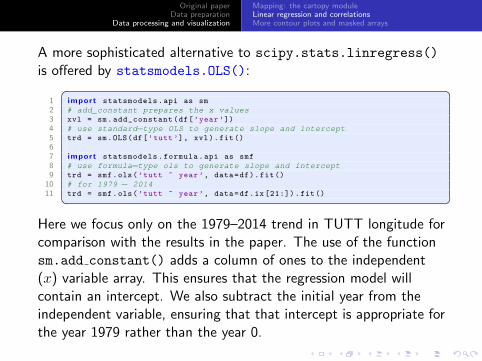
A more sophisticated alternative to scipy.stats.linregress()
is offered by statsmodels.OLS():� �1 import statsmodels.api as sm
2 # add_constant prepares the x values3 xvl = sm.add_constant(df[’year’])
4 # use standard−type OLS to generate slope and intercept5 trd = sm.OLS(df[’tutt’], xvl).fit()
67 import statsmodels.formula.api as smf
8 # use formula−type ols to generate slope and intercept9 trd = smf.ols(’tutt ~ year’, data=df).fit()
10 # for 1979 − 201411 trd = smf.ols(’tutt ~ year’, data=df.ix [21:]).fit()� �
Here we focus only on the 1979–2014 trend in TUTT longitude forcomparison with the results in the paper. The use of the functionsm.add constant() adds a column of ones to the independent(x) variable array. This ensures that the regression model willcontain an intercept. We also subtract the initial year from theindependent variable, ensuring that that intercept is appropriate forthe year 1979 rather than the year 0.
Original paperData preparation
Data processing and visualization
Mapping: the cartopy moduleLinear regression and correlationsMore contour plots and masked arrays
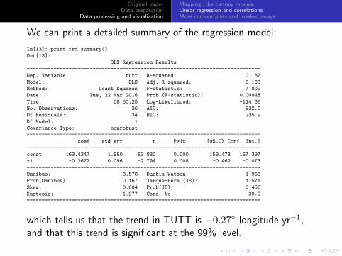
We can print a detailed summary of the regression model:
In[13]: print trd.summary()
Out[13]:
OLS Regression Results
==============================================================================
Dep. Variable: tutt R-squared: 0.187
Model: OLS Adj. R-squared: 0.163
Method: Least Squares F-statistic: 7.809
Date: Tue, 22 Mar 2016 Prob (F-statistic): 0.00848
Time: 08:50:25 Log-Likelihood: -114.38
No. Observations: 36 AIC: 232.8
Df Residuals: 34 BIC: 235.9
Df Model: 1
Covariance Type: nonrobust
==============================================================================
coef std err t P>|t| [95.0% Conf. Int.]
------------------------------------------------------------------------------
const 163.4347 1.950 83.830 0.000 159.473 167.397
x1 -0.2677 0.096 -2.794 0.008 -0.462 -0.073
==============================================================================
Omnibus: 3.578 Durbin-Watson: 1.963
Prob(Omnibus): 0.167 Jarque-Bera (JB): 1.571
Skew: 0.004 Prob(JB): 0.456
Kurtosis: 1.977 Cond. No. 39.9
==============================================================================
which tells us that the trend in TUTT is −0.27◦ longitude yr−1,and that this trend is significant at the 99% level.
Original paperData preparation
Data processing and visualization
Mapping: the cartopy moduleLinear regression and correlationsMore contour plots and masked arrays
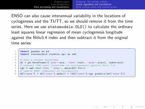
ENSO can also cause interannual variability in the locations ofcyclogenesis and the TUTT, so we should remove it from the timeseries. Here we use statsmodels.OLS() to calculate the ordinaryleast squares linear regression of mean cyclogenesis longitudeagainst the Nino3.4 index and then subtract it from the originaltime series:� �
1 import pandas as pd
2 import statsmodels.formula.api as smf
34 # make a pandas dataframe5 df = pd.DataFrame ({’jtwc’:mln , ’tutt’:tutt , ’nino’:nino}, index=yrs)
6 # regress JTWC mean longitude of cyclogenesis against Nino 3.47 rgr = smf.ols(’jtwc ~ nino’, data=df).fit()
8 # remove ENSO component of variability9 df[’estm’] = df[’jtwc’].mean() + (df[’jtwc’]-rgr.predict(df[’nino’]))� �

Original paperData preparation
Data processing and visualization
Mapping: the cartopy moduleLinear regression and correlationsMore contour plots and masked arrays
1960 1970 1980 1990 2000 2010Year
120
130
140
150
160
TC m
ean
gene
sis
long
itude
[°E
]
JTWC (original)JTWC (ENSO influence removed)
Although ENSO affects the year-to-year variability, the trend withENSO removed (−0.11◦ longitude yr−1) is within the 95%confidence interval around the original trend (−0.14± 0.14◦
longitude yr−1), so we can neglect ENSO effects.
Original paperData preparation
Data processing and visualization
Mapping: the cartopy moduleLinear regression and correlationsMore contour plots and masked arrays
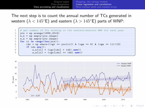
The next step is to count the annual number of TCs generated inwestern (λ < 145◦E) and eastern (λ > 145◦E) parts of WNP:� �
1 # get number of TCs forming in the eastern/western WNP for each year2 yrs = np.arange (1958 ,2015)
3 w_n = np.empty(yrs.shape)
4 e_n = np.empty(yrs.shape)
5 f o r ii i n range ( l e n (yrs)):6 idx = np.where ((cgt == yrs[ii]) & (cgm >= 6) & (cgm <= 11))[0]
7 i f idx.any():8 w_n[ii] = (cgx[idx] < 145).sum()
9 e_n[ii] = (cgx[idx] >= 145).sum()� �
1960 1970 1980 1990 2000 20100
5
10
15
20
25
30
TC c
ount
R = −0.27
Western WNPEastern WNP
Original paperData preparation
Data processing and visualization
Mapping: the cartopy moduleLinear regression and correlationsMore contour plots and masked arrays
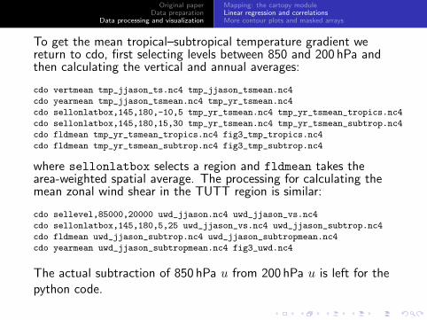
To get the mean tropical–subtropical temperature gradient wereturn to cdo, first selecting levels between 850 and 200 hPa andthen calculating the vertical and annual averages:
cdo vertmean tmp_jjason_ts.nc4 tmp_jjason_tsmean.nc4
cdo yearmean tmp_jjason_tsmean.nc4 tmp_yr_tsmean.nc4
cdo sellonlatbox,145,180,-10,5 tmp_yr_tsmean.nc4 tmp_yr_tsmean_tropics.nc4
cdo sellonlatbox,145,180,15,30 tmp_yr_tsmean.nc4 tmp_yr_tsmean_subtrop.nc4
cdo fldmean tmp_yr_tsmean_tropics.nc4 fig3_tmp_tropics.nc4
cdo fldmean tmp_yr_tsmean_subtrop.nc4 fig3_tmp_subtrop.nc4
where sellonlatbox selects a region and fldmean takes thearea-weighted spatial average. The processing for calculating themean zonal wind shear in the TUTT region is similar:
cdo sellevel,85000,20000 uwd_jjason.nc4 uwd_jjason_vs.nc4
cdo sellonlatbox,145,180,5,25 uwd_jjason_vs.nc4 uwd_jjason_subtrop.nc4
cdo fldmean uwd_jjason_subtrop.nc4 uwd_jjason_subtropmean.nc4
cdo yearmean uwd_jjason_subtropmean.nc4 fig3_uwd.nc4
The actual subtraction of 850 hPa u from 200 hPa u is left for thepython code.

Original paperData preparation
Data processing and visualization
Mapping: the cartopy moduleLinear regression and correlationsMore contour plots and masked arrays
1960 1970 1980 1990 2000 2010Year
0.0
0.3
0.6
0.9
1.2
1.5
1.8
2.1
Tem
pera
ture
gra
dien
t [K
]
R = 0.97
0
2
4
6
8
10
12
14
Zona
l win
d sh
ear [
m s−
1 ]
The strong relationship between these two time series is consistentwith the hypothesis that interannual variability and trends in windshear (and hence the preferred location of cyclogenesis) in thisregion are driven by the thermal wind relationship.
Original paperData preparation
Data processing and visualization
Mapping: the cartopy moduleLinear regression and correlationsMore contour plots and masked arrays
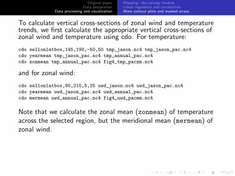
To calculate vertical cross-sections of zonal wind and temperaturetrends, we first calculate the appropriate vertical cross-sections ofzonal wind and temperature using cdo. For temperature:
cdo sellonlatbox,145,190,-50,50 tmp_jason.nc4 tmp_jason_pac.nc4
cdo yearmean tmp_jason_pac.nc4 tmp_annual_pac.nc4
cdo zonmean tmp_annual_pac.nc4 fig4_tmp_paczm.nc4
and for zonal wind:
cdo sellonlatbox,90,210,5,25 uwd_jason.nc4 uwd_jason_pac.nc4
cdo yearmean uwd_jason_pac.nc4 uwd_annual_pac.nc4
cdo mermean uwd_annual_pac.nc4 fig4_uwd_pacmm.nc4
Note that we calculate the zonal mean (zonmean) of temperatureacross the selected region, but the meridional mean (mermean) ofzonal wind.

Original paperData preparation
Data processing and visualization
Mapping: the cartopy moduleLinear regression and correlationsMore contour plots and masked arrays
To calculate trends in a time series effectively, we can define afunction that uses statsmodels.OLS():� �
1 import statsmodels.api as sm
23 # function to calculate trend and significance from a pandas time series4 def pdtrend(x,ci =0.95):
5 """6 A basic function for calculating trends given a pandas time7 series.89 Variables:
10 x :: the series1112 Parameters:13 ci :: confidence interval for significance testing14 """15 # statsmodels regression require us to add a constant16 xvl = sm.add_constant(np.array(x.index))
17 # ordinary least squares linear regression18 rgr = sm.OLS(x.values ,xvl).fit()
19 # trend slope (per year in this case)20 trnd = rgr.params [1]
21 # simple representation of statistical significance (True/False)22 tsig = (rgr.pvalues [1] < (1-ci))
23 r e t u r n (trnd , tsig)� �

Original paperData preparation
Data processing and visualization
Mapping: the cartopy moduleLinear regression and correlationsMore contour plots and masked arrays
An important note at this point: the example paper we are workingfrom uses a non-parametric Mann-Kendall test, and accounts forauto-correlation in the time series in significance testing. Thefunction on the previous page uses Student’s t test, which is (a)parametric and (b) assumes that the underlying data are normallydistributed. We have also not adjusted the effective sample size toaccount for auto-correlation. Our approach is acceptable forexploratory analysis, but would be unsuitable for publication-qualitywork. The reason that we have used a function in this case is thatthis makes it easier to later add or modify the criteria for statisticalsignificance to make them more sophisticated or data-aware. Formore details, see Chapter 17 of Statistical Analysis in ClimateResearch by Hans von Storch and Francis W. Zwiers.
Original paperData preparation
Data processing and visualization
Mapping: the cartopy moduleLinear regression and correlationsMore contour plots and masked arrays
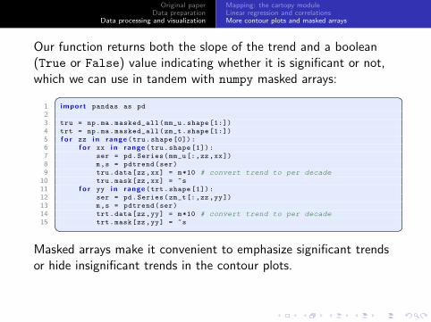
Our function returns both the slope of the trend and a boolean(True or False) value indicating whether it is significant or not,which we can use in tandem with numpy masked arrays:� �
1 import pandas as pd
23 tru = np.ma.masked_all(mm_u.shape [1:])
4 trt = np.ma.masked_all(zm_t.shape [1:])
5 f o r zz i n range (tru.shape [0]):6 f o r xx i n range (tru.shape [1]):7 ser = pd.Series(mm_u[:,zz,xx])
8 m,s = pdtrend(ser)
9 tru.data[zz,xx] = m*10 # convert trend to per decade10 tru.mask[zz,xx] = ~s
11 f o r yy i n range (trt.shape [1]):12 ser = pd.Series(zm_t[:,zz,yy])
13 m,s = pdtrend(ser)
14 trt.data[zz,yy] = m*10 # convert trend to per decade15 trt.mask[zz,yy] = ~s� �
Masked arrays make it convenient to emphasize significant trendsor hide insignificant trends in the contour plots.

Original paperData preparation
Data processing and visualization
Mapping: the cartopy moduleLinear regression and correlationsMore contour plots and masked arrays
100°E 120°E 140°E 160° 180°1000
850
700
500
400
300
250
200
150
100
Pre
ssur
e [h
Pa]
1.0
0.5
0.0
0.5
1.0
Tren
d in
zon
al w
ind
[m s−
1 de
c−1 ]
45°S 30°S 15°S 0° 15°N 30°N 45°N1000
850
700
500
400
300
250
200
150
100
Pre
ssur
e [h
Pa]
0.5
0.4
0.3
0.2
0.1
0.0
0.1
0.2
0.3
0.4
0.5
Tren
d in
tem
pera
ture
[K d
ec−
1 ]
� �1 cs1 = ax.contour(jlon , jlev , mm_u.mean(axis =0), np.arange (-50,50,2),
2 colors=’k’)
3 cs2 = ax.contourf(jlon , jlev , tru.data , np.linspace (-1,1,11),
4 cmap=plt.cm.RdBu_r , extend=’both’)
5 ax.contourf(jlon , jlev , tru.mask.astype(’int’), [-0.5,0.5],
6 hatches =[’xx’,’none’], colors=’none’, edgecolor=’#666666 ’,
7 zorder =10)
8 cb = plt.colorbar(cs2 , orientation=’vertical ’, extend=’both’, aspect =50)
9 cb.set_ticks ([-1,-0.5,0,0.5,1])
10 cb.set_label(’Trend in zonal wind [m s$^{-1}$ dec$ ^{-1}$]’)� �
Original paperData preparation
Data processing and visualization
Mapping: the cartopy moduleLinear regression and correlationsMore contour plots and masked arrays
100°E 120°E 140°E 160° 180°1000
850
700
500
400
300
250
200
150
100
Pre
ssur
e [h
Pa]
1.0
0.5
0.0
0.5
1.0
Tren
d in
zon
al w
ind
[m s−
1 de
c−1 ]
45°S 30°S 15°S 0° 15°N 30°N 45°N1000
850
700
500
400
300
250
200
150
100
Pre
ssur
e [h
Pa]
0.5
0.4
0.3
0.2
0.1
0.0
0.1
0.2
0.3
0.4
0.5
Tren
d in
tem
pera
ture
[K d
ec−
1 ]
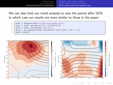
We can also limit our trend analysis to only the period after 1979,in which case our results are more similar to those in the paper.� �
1 ncdf = Dataset(ddir+’fig4_uwd_pacmm.nc4’)
2 jlev = ncdf.variables[’lev’][:27]*0.01
3 jlon = ncdf.variables[’lon’][:]
4 mm_u = np.squeeze(ncdf.variables[’ugrd’][21: ,:27 ,: ,:])
5 ncdf.close()� �


![Mesoscale Cyclogenesis Dynamics Over the Southwestern Ross ...polarmet.osu.edu/PMG_publications/carrasco_bromwich_jgr_1993.pdf · Cyclogenesis studies [Brom•4ch, 1989b, 1991] during](https://img.dokumen.tips/doc/110x75/60b12b7d37f70d6cc938121a/mesoscale-cyclogenesis-dynamics-over-the-southwestern-ross-cyclogenesis-studies.jpg)