Embed Size (px)
Citation preview

USDA/DOE Bioenergy Contract Number: DE-PS36-06GO96002F 1
Western Governors’ Association:
Strategic Development of Bioenergy in the Western States
Development of Supply Scenarios Linked to Policy Recommendations
Task 3:
Spatial Analysis and Supply Curve Development
Subcontractor: University of California, Davis
FINAL REPORT
June 2008
USDA/DOE Bioenergy Contract Number: DE-PS36-06GO96002F 2
Abstract Uncertainties in the contribution that biofuels might make in meeting the energy
needs of the transportation sector in the western US by 2015 were addressed by combining a spatially-explicit resource inventory and assessment, models of conversion technologies, and transportation costs into an integrated model of biofuel supply chains. Geographic Information System (GIS) modeling was used in conjunction with an infrastructure system cost optimization model to develop biofuel supply curves using biomass feedstocks throughout the western US. Biofuels could provide between 5 and 10 percent of the projected transportation fuel demand in the region with fuel price between $2.40 and $3.00 per gasoline gallon equivalence (gge) excluding local distribution costs and taxes. A diverse resource base is relied on to provide this fuel with significant contributions from municipal solid waste, agricultural residue, herbaceous energy crop, forest thinning, corn, and lipid resources. The biofuel potential estimated in this way is significant, but substantial uncertainties remain. In interpreting the supply estimates, unresolved questions remain regarding economic performance of the different conversion technologies and the overall sustainability of many of the biomass resources considered.
USDA/DOE Bioenergy Contract Number: DE-PS36-06GO96002F 3
Table of Contents Abstract……………………………………………………………………………………2 Contributors……………………………………………………………………………… 4 Acknowledgements………………………………………………………………………. 4 List of Tables…………………………………………………………………………….. 5 List of Figures……………………………………………………………………………. 5 1 Introduction................................................................................................................... 7 2 Objectives – Task 3....................................................................................................... 8 3 Methods......................................................................................................................... 9
3.1 GIS Model Development ..................................................................................... 12 3.1.1 Database resources and development ........................................................... 13 3.1.2 Biomass Resource Mapping ......................................................................... 15 3.1.3 Siting Criteria for Biorefineries .................................................................... 16 3.1.4 Network Modeling........................................................................................ 18
3.2 Cost Models ......................................................................................................... 19 3.2.1 Conversion Technologies and Costs............................................................. 20 3.2.2 Transportation Costs ..................................................................................... 23
3.3 Facility Optimization ........................................................................................... 26 3.3.1 Modeling Approach ...................................................................................... 26 3.3.2 Model Derivation and Solution Procedure ................................................... 27
4 Results......................................................................................................................... 29 4.1 Biomass Resources .............................................................................................. 29
4.1.1 Biomass Supply by Procurement Cost.......................................................... 29 4.1.2 Biomass Resource Maps ............................................................................... 30
4.2 Regional Biofuel Supply Curves ......................................................................... 34 4.3 Target Price Results ............................................................................................. 37
4.3.1 Target Price................................................................................................... 37 4.3.2 Mapping Biofuel Industry in Western United States at Target Price ........... 38 4.3.3 Supply Maps by State ................................................................................... 38 4.3.4 Detailed Target Price Results........................................................................ 40
4.4 Sensitivity Analysis ............................................................................................. 43 5 Discussion................................................................................................................... 50
5.1 Important Factors Determining Supply ............................................................... 50 5.2 Relevance to Existing Policies............................................................................. 50 5.3 Model Limitations................................................................................................ 52
6 Conclusions................................................................................................................. 54 7 References................................................................................................................... 55 8 Appendices.................................................................................................................. 57
8.1 Appendix A: Details of Supply Chain Optimization Model................................ 57 8.2 Appendix B: State Atlas....................................................................................... 59
USDA/DOE Bioenergy Contract Number: DE-PS36-06GO96002F 4
Contributors • The University of California, Davis (UC Davis):
• Nathan Parker, Graduate Student Researcher, Institute of Transportation Studies • Peter Tittmann, Graduate Student Researcher, Department of Geography • Quinn Hart, Programmer, Department of Land, Air and Water Resources • Mui Lay, Programmer, Department of Land, Air and Water Resources • Joshua Cunningham, Program Manager – STEPS, Institute of Transportation
Studies • Bryan Jenkins, Professor, Department of Biological and Agricultural
Engineering
• Kansas State University (KSU): • Richard Nelson, Director and Department Head, Engineering Extension
• U.S. Forest Service (USFS):
• Ken Skog, Forest Products Laboratory
• National Renewable Energy Laboratory (NREL): • Anelia Milbrandt
• Antares Group, Inc.:
• Ed Gray, President • Anneliese Schmidt, Renewable Research Scientist
Acknowledgements The authors of this study would like to thank Gayle Gordon, Western Governors’ Association, and Ed Gray, President, Antares Group, for initiating and managing the Strategic Development of Bioenergy in the Western States project. The authors also thank the following organizations for their technical and financial support, without which this study could not have been completed.
• Western Governors’ Association • United States Department of Agriculture • United States Department of Energy • Antares Group, Inc. • National Renewable Energy Laboratory • California Energy Commission • Public Interest Energy Research Program • California Biomass Collaborative • University of California, Davis Department of Biological and Agricultural Engineering Geography Graduate Group Department of Land, Air, and Water Resources Center for Spatial Technologies and Remote Sensing Institute of Transportation Studies Energy Institute
USDA/DOE Bioenergy Contract Number: DE-PS36-06GO96002F 5
List of Tables Table 1: Biofuel Pathways Modeled................................................................................. 10 Table 2: Biomass Feedstock Data..................................................................................... 14 Table 3: Criteria for Potential Biorefinery Locations. ...................................................... 16 Table 4: Annualized Conversion Costs for Biofuel Technologies Analyzed ................... 22 Table 5: Assumed Conversion Efficiencies for Technologies by Biomass Type............. 22 Table 6: Energy Content of Biofuels ................................................................................ 23 Table 7: Road Travel Speed from NHPN........................................................................ 24 Table 8: Trucking Costs.................................................................................................... 24 Table 9: Moisture Content of Biomass and Density of Liquid Feedstocks ...................... 24 Table 10: Rail Transportation Costs ................................................................................. 25 Table 11: Marine Transportation Costs ............................................................................ 26 Table 12: Feedstock Consumed in Target Price Configuration........................................ 41

USDA/DOE Bioenergy Contract Number: DE-PS36-06GO96002F 6
List of Figures Figure 1: Biofuel Supply Chain....................................................................................................... 9 Figure 2: GIS Model Structure ...................................................................................................... 12 Figure 3: GIS Transportation Network.......................................................................................... 13 Figure 4: Seed oils accumulation .................................................................................................. 15 Figure 5: Biorefinery Siting Criteria ............................................................................................. 17 Figure 6: Potential Biorefinery Locations ..................................................................................... 18 Figure 7: Potential Biorefinery Sites and Nearest Terminal.......................................................... 19 Figure 8: Linear Fit for the Annualized Cost of Production for FT Diesel ................................... 20 Figure 9: Linear fit to model estimate for economies of scale. ..................................................... 21 Figure 10: Rate for Rail Transportation ........................................................................................ 25 Figure 11: Simplified Model Schematic........................................................................................ 27 Figure 12: Supply Curve Generation............................................................................................. 28 Figure 13: Lignocellulosic Biomass Resource Supply by Procurement Cost ............................... 29 Figure 14: Oil Biomass Resource Supply by Procurement Cost................................................... 30 Figure 15: Map of Corn Resources ............................................................................................... 31 Figure 16: Map of Lignocellulosic Feedstock Resources ............................................................ 32 Figure 17: Map of Vegetable and Waste Oil Feedstock Resources .............................................. 33 Figure 18: Regional Supply Curve for Biofuels............................................................................ 35 Figure 19: Supply Curve for Gasoline-Replacement Biofuels ...................................................... 36 Figure 20: Supply Curve for Diesel-Replacement Biofuels .......................................................... 36 Figure 21: Biomass Supply at Biofuel Price by Type of Biomass ................................................ 37 Figure 22: Map of biofuels production in the Western Governors Association region................. 38 Figure 23: Map of biofuels production in Kansas for a target price of $2.40/gge......................... 39 Figure 24: Breakdown of Biofuels Produced at Target Price........................................................ 40 Figure 25: Feedstock Consumption at Target Price ...................................................................... 41 Figure 26: Breakdown of Costs for Biofuels Produced................................................................. 42 Figure 27: Procurement Cost for Lignocellulosic Resources used in Target Price Configuration 43 Figure 28: Effect of "High Forest" Resource Assessment on Biofuel Supply .............................. 44 Figure 29: Effect of Corn Price on Biofuel Supply ....................................................................... 46 Figure 30: Effect of Excluding Corn, Oil Seeds and Herbaceous Energy Crops on Biofuel Supply....................................................................................................................................................... 47 Figure 31: Effect of Stalled LCE Technology on Biofuel Supply................................................. 48 Figure 32: Effect of Maximum LCE Biorefinery Size on Supply Curve ...................................... 49 Figure 33: Renewable Fuel Standard (RFS) included in EISA 2007 ............................................ 52

USDA/DOE Bioenergy Contract Number: DE-PS36-06GO96002F 7
1 Introduction The goal of the Strategic Development of Bioenergy in the Western States project is
to provide the Western Governor’s Association (WGA) and their respective state energy policy organizations and legislatures a clear understanding of the contribution that bioenergy (fuels, electricity and thermal energy) can make to energy requirements of the western United States by 2015 and provide a recommended policy framework to create the environment in which bioenergy projects can appropriately develop.
This strategic analysis addresses the following questions: 1. What contributions to energy supply can bioenergy make by 2015? The WGA’s
Clean and Diversified Energy Advisory Committee’s (CDEAC) Biomass Task Force has already answered the question in large part for electricity from biomass. This project attempts to provide relevant analysis for the question of biofuels.
2. What are the barriers to achieving the full potential of bioenergy supply? 3. What is the full set of policy measures and incentives that would enable this
transformation to significantly increase bioenergy supply? What is the likely path for implementing these measures? In particular, what impact would bioenergy development have on the success of meeting the goals of the Healthy Forest Initiative and similar federal and state policy objectives?
4. What is the potential cost for these measures, and what are the impacts and benefits?
5. What are the regional differences within the western US with regard to capability to produce bioenergy – how do these differences influence individual state strategies? Which resources should be developed first – which ones will take more time?
6. What is the technology progression and sequence for the transition from today’s technology and processes to tomorrow’s vision?
7. What is the variation in resource by region – how does that inform policy and resource development choices?
This report addresses the task of estimating the resource and biofuel supply potentials along with the costs of production. These estimates derive from detailed geographic information system (GIS) and cost optimization models. Results included here are in some measures preliminary but provide insight into model development and the relative magnitude of the biofuel supply that might be generated from biomass resources in the western United States. The methods and data employed are still undergoing development. Extensions of the models described here to include the entire U.S. are currently in progress, and results will be described in future reports.

USDA/DOE Bioenergy Contract Number: DE-PS36-06GO96002F 8
2 Objectives – Task 3 The primary objective of this task was to prepare biofuel supply curves estimating
potential future supplies of liquid fuels from biomass in the western U.S. as a function of market price. To accomplish this objective, a combined GIS network analysis and biorefinery optimization model was developed to:
• spatially resolve biomass resource quantities and distributions throughout the WGA region for major feedstock types,
• map supporting transportation and biofuel handling infrastructure for the purposes of estimating biorefinery-gate feedstock costs and biofuel distribution costs,
• optimize biorefinery types, sizes, and locations for competing conversion technologies based on the objective of maximizing producer profit under a market price constraint.
The analysis focuses on the generation of biomass and biofuel supply curves over a Year 2015 planning horizon.

USDA/DOE Bioenergy Contract Number: DE-PS36-06GO96002F 9
3 Methods We have developed a methodology that combines optimization methods from operations research and the geographic tools available through Geographic Information Systems (GIS) into an integrated model of the biofuel industry. The integrated model analyzes biofuel supply chains from the field or other biomass source to the fuel distribution terminal. The industry is modeled as a profit maximizing entity that knows all the costs and prices that are relevant to the industry. This simplification allows the model to use the rich geographic data to find what a biofuels industry would look like under a relatively limited set of parameters. The resulting biofuels industry is described in the results by the locations, sizes and types of biorefineries built as well as identifying the biomass resources that are used by each biorefinery.
Figure 1: Biofuel Supply Chain
This work builds upon previous work in the areas of biomass resource assessment, bioenergy facility location, and facility siting in general, including the work by Oak Ridge National Laboratory (ORNL) among others [1, 2]. The most recent national assessment [1] did not include an explicit economic component. A number of models have been developed that can be used for biorefinery siting using geographic resource assessments. Graham et al [3] developed a GIS model that optimally locates biorefineries of a given feedstock input based on the marginal cost of an energy crop feedstock delivered to the site. Biorefineries are located sequentially to avoid over-allocation or double-counting of the resources. The method was demonstrated using a case study of switchgrass in Tennessee. Kaylen et al [4] incorporate the competition between the economies of scale in production against the transportation cost of the biomass feedstock using a nonlinear programming model for a single lignocellulosic

USDA/DOE Bioenergy Contract Number: DE-PS36-06GO96002F 10
ethanol facility location and sizing problem. Freppaz et al [5] developed a decision support system (DSS) to aid regional authorities in making the most of their forest resources for heat and electricity generation. The work of one of the authors [6] designing agricultural waste to hydrogen supply chains from fields to pump using a mixed integer non-linear model has been adapted for considering multiple fuel pathways over a significantly larger geographic extent for the WGA project.
We have addressed the competition for feedstock between locations and the tradeoff between economies of scale and feedstock delivered cost through simultaneous biorefinery siting, sizing and allocation of resources. We consider multiple fuel pathways and the entire WGA region, a large geographic scope, is included in one optimization model allowing for trading between states. Matching this powerful analysis tool with a set of consistent and current resource assessments provides a method for in-depth analysis of bioenergy alternatives in the West.
From the large set of possible biofuel pathways, we have chosen to model 30 pathways consisting of 12 feedstock types and 6 biofuel conversion technologies. The feedstock types can be grouped into three categories – lignocellulosics, oils and other lipids, and grains (Table 1). So-called clean biomass constitutes a subset of the lignocellulosic category. Three technologies are capable of exploiting the lignocellulosic resources – Fischer Tropsch diesel (LCMD), upgrading of pyrolysis oil to gasoline in a centralized production/refining model (LCG), and cellulosic ethanol through hydrolysis and fermentation (LCE), which is limited to the clean fraction of the resource. Two technologies are considered for conversion of oils to diesel-replacement fuels – fatty acid to methyl esters (FAME) and hydrotreatment (FAHC). Corn, the only grain feedstock considered, is included for production of ethanol through both wet- and dry-milling processes. More detailed information on the conversion technologies is given in the Task 2 report [7] and feedstock supply data are described in the Task 1 report [8]. Table 1: Biofuel Pathways Modeled
Feedstock Category Feedstock Type Conversion Technologies
Clean Lignocellulosics
Forest biomass Herbaceous Energy Crops
Straw and Stover Ag. Residues Orchard/Vineyard Wastes
Municipal Solid Wastes (MSW) • Clean Mixed Paper • Clean Wood Wastes
Clean Yard Wastes
LCE LCG
LCMD
Lignocellulosics Remainder of Biomass MSW, Remainder from sorting
LCG LCMD
Lipids Seed Oils
Yellow Grease Animal Fats
FAME FAHC
Grains Corn Dry Mill Ethanol Wet Mill Ethanol

USDA/DOE Bioenergy Contract Number: DE-PS36-06GO96002F 11
As noted earlier, in deriving biofuel supply curves, a model framework was created which can optimize the siting of biofuel production facilities in the western United States. The conditions for optimality are the availability of feedstock; the distance the feedstock has to travel to reach the facility gate; the capital, operating, and maintenance costs of the facility; and the distance the product has to travel to reach fuel distribution terminals. The variety of feedstock types and conversion methods available for producing biofuels make this a challenging task. The model is designed to address the following two questions:
1. To produce n million gallons/year of x (biofuel), what are the optimal locations, sizes and number of facilities capable of producing x?
2. To produce N MJ of energy as liquid biofuel, what are the optimal sizes, locations, and type of plant to accomplish this?
There are four primary costs required by this model:
1. Harvest or collection cost: The cost to procure feedstock from the site of origin.
2. Transport cost: The cost to load and transport feedstock from its origin to the biorefinery, and the cost to transport the final product from the biorefinery to the distribution terminal.
3. Conversion cost: The cost to convert the raw feedstock into a usable liquid fuel.
4. Distribution cost: The cost to bring the biofuel to market at a fuel distribution terminal.
To generate accurate transportation costs, all input data must be attributed to a specific geographic location. Feedstocks were located to a county or municipality depending upon type. We used simple initial criteria for identifying the general potential location of biorefineries which resulted in 291 representative potential locations (see Section 3.1.3 for detail). Spatial data were manipulated with ESRI’s ArcGIS Geographic Information Systems (GIS) software [9] and the PostgreSQL database with PostGIS extension [10]. To determine transportation costs and distances, least-cost pathways were calculated using network analysis. To calculate optimality for the system, all cost data were input into a mixed integer-linear optimization model created in the General Algebraic Modeling System (GAMS) (Figure 2).

USDA/DOE Bioenergy Contract Number: DE-PS36-06GO96002F 12
Figure 2: GIS Model Structure
3.1 GIS Model Development The purpose of the GIS model is to supply inputs to the GAMS optimization model. These inputs include: the total amounts of various feedstocks available; potential biorefinery locations; transportation costs from feedstock sources to potential biorefinery locations; and transportation costs from biorefineries to terminals. In addition, oil seed feedstock supplies, canola and soybean, require an additional processing step of oil extraction. The GIS model is used to account for that process as well. The transportation network includes road, rail, and marine transportation, with specified intermodal facilities capable of loading and unloading bulk dry and liquid products. Figure 3 shows the connections between the various stages of biofuel production.
A significant number of the feedstock sources are only defined at the county level. For transportation costs, a simple intra-county cost has been applied, based on the size of the county. Because of this, all feedstock sources are identified as point sources.

USDA/DOE Bioenergy Contract Number: DE-PS36-06GO96002F 13
Figure 3: GIS Transportation Network
3.1.1 Database resources and development Biomass feedstock data were compiled from a variety of sources (Table 2). Data on the majority of the agricultural crops and residues as well as waste grease, beef tallow, and pork lard were provided by Dr. Richard Nelson, Kansas State University [8]. Forestry data were provided by the Forest Products Laboratory of the US Forest Service for a base case and a “high” supply scenarios [8]. Supply data for municipal solid waste and orchard and vineyard residues were compiled from a previous CDEAC study on electricity potential from biomass [11]. Each dataset contained either a supply curve indicating the quantity available at a given price or a single cost/volume. Only orchard and vineyard residues were assumed to be available at no cost at the roadside.

USDA/DOE Bioenergy Contract Number: DE-PS36-06GO96002F 14
Table 2: Biomass Feedstock Data
Feedstock Type Feedstock Category Geography Source
Winter wheat straw agricultural cellulosic county Kansas State Extension
Spring wheat straw agricultural cellulosic county Kansas State Extension
Corn stover agricultural cellulosic county Kansas State Extension
Barley straw agricultural cellulosic county Kansas State Extension
Oat straw agricultural cellulosic county Kansas State Extension
Rye straw agricultural cellulosic county Kansas State Extension
Orchard and vineyard agricultural cellulosic county WGA CDEAC (Bioenergy)
Corn grain grain county Kansas State Extension
Canola lipid county Kansas State Extension
Soybean lipid county Kansas State Extension
Beef tallow lipid county Kansas State Extension
Pork lard lipid county Kansas State Extension
Fire hazard thinning woody cellulosic county USFS Forest Products Lab
Logging residue woody cellulosic county USFS Forest Products Lab
Pinyon Juniper woody cellulosic county USFS Forest Products Lab
Private timberland thinning except lodgepole & spruce fir
woody cellulosic county USFS Forest Products Lab
Private timberland thinning - lodgepole & spruce fir only
woody cellulosic county USFS Forest Products Lab
Insect and disease thinning woody cellulosic county USFS Forest Products Lab
Pre-commercial thinning on National Forests in western
OR and WA counties
woody cellulosic county USFS Forest Products Lab
Unused mill residue woody cellulosic county USFS Forest Products Lab
Municipal solid waste solid waste municipality WGA CDEAC (Bioenergy)
Waste grease lipid municipality Kansas State Extension
USDA/DOE Bioenergy Contract Number: DE-PS36-06GO96002F 15
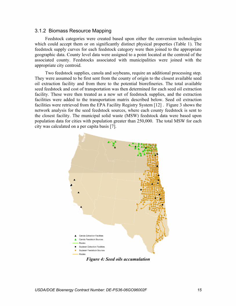
3.1.2 Biomass Resource Mapping Feedstock categories were created based upon either the conversion technologies which could accept them or on significantly distinct physical properties (Table 1). The feedstock supply curves for each feedstock category were then joined to the appropriate geographic data. County level data were assigned to a point located at the centroid of the associated county. Feedstocks associated with municipalities were joined with the appropriate city centroid.
Two feedstock supplies, canola and soybeans, require an additional processing step. They were assumed to be first sent from the county of origin to the closest available seed oil extraction facility and from there to the potential biorefineries. The total available seed feedstock and cost of transportation was then determined for each seed oil extraction facility. These were then treated as a new set of feedstock supplies, and the extraction facilities were added to the transportation matrix described below. Seed oil extraction facilities were retrieved from the EPA Facility Registry System [12] . Figure 3 shows the network analysis for the seed feedstock sources, where each county feedstock is sent to the closest facility. The municipal solid waste (MSW) feedstock data were based upon population data for cities with population greater than 250,000. The total MSW for each city was calculated on a per capita basis [7].
Figure 4: Seed oils accumulation
USDA/DOE Bioenergy Contract Number: DE-PS36-06GO96002F 16
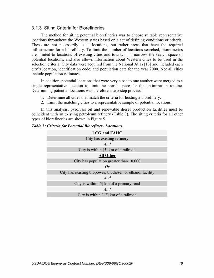
3.1.3 Siting Criteria for Biorefineries The method for siting potential biorefineries was to choose suitable representative locations throughout the Western states based on a set of defining conditions or criteria. These are not necessarily exact locations, but rather areas that have the required infrastructure for a biorefinery. To limit the number of locations searched, biorefineries are limited to locations of existing cities and towns. This narrows the search space of potential locations, and also allows information about Western cities to be used in the selection criteria. City data were acquired from the National Atlas [13] and included each city’s location, identification code, and population data for the year 2000. Not all cities include population estimates.
In addition, potential locations that were very close to one another were merged to a single representative location to limit the search space for the optimization routine. Determining potential locations was therefore a two-step process:
1. Determine all cities that match the criteria for hosting a biorefinery. 2. Limit the matching cities to a representative sample of potential locations.
In this analysis, pyrolysis oil and renewable diesel production facilities must be coincident with an existing petroleum refinery (Table 3). The siting criteria for all other types of biorefineries are shown in Figure 5.
Table 3: Criteria for Potential Biorefinery Locations.
LCG and FAHC City has existing refinery
And City is within [5] km of a railroad
All Other City has population greater than 10,000
Or City has existing biopower, biodiesel, or ethanol facility
And City is within [5] km of a primary road
And City is within [12] km of a railroad
USDA/DOE Bioenergy Contract Number: DE-PS36-06GO96002F 17
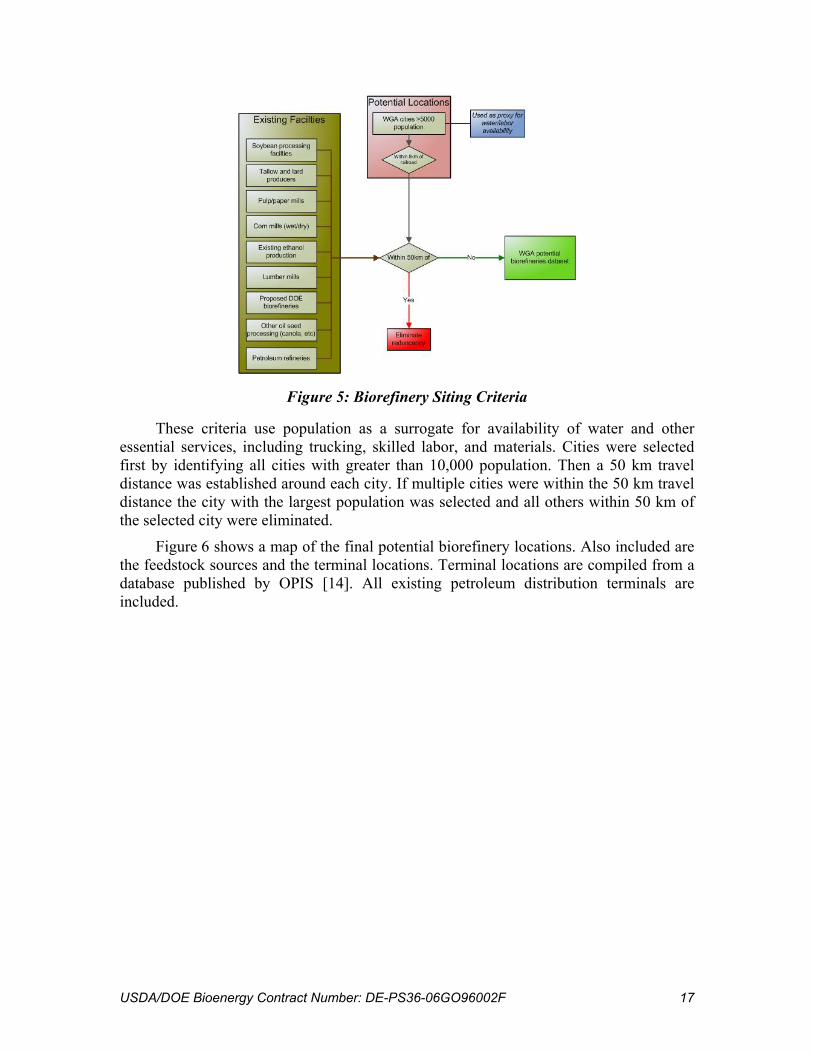
Figure 5: Biorefinery Siting Criteria
These criteria use population as a surrogate for availability of water and other essential services, including trucking, skilled labor, and materials. Cities were selected first by identifying all cities with greater than 10,000 population. Then a 50 km travel distance was established around each city. If multiple cities were within the 50 km travel distance the city with the largest population was selected and all others within 50 km of the selected city were eliminated.
Figure 6 shows a map of the final potential biorefinery locations. Also included are the feedstock sources and the terminal locations. Terminal locations are compiled from a database published by OPIS [14]. All existing petroleum distribution terminals are included.

USDA/DOE Bioenergy Contract Number: DE-PS36-06GO96002F 18
Figure 6: Potential Biorefinery Locations
3.1.4 Network Modeling To accurately calculate the costs of transporting feedstock and fuels along the supply
chain, a comprehensive transportation network was assembled. The transportation network includes existing highways, rail lines, and marine transport routes, as well as inter-modal facilities. The underlying network data were assembled from Bureau of Transportation Statistics sources [15-18]. The inclusion of inter-modal facilities allows for the calculation of loading and unloading costs associated with the transfer of feedstock or fuel from one mode of transport to another. The network was built to enable the calculation of both time and cost of travel between two locations. Thus, each segment of the network is attributed with a mode and speed of travel.
Data from a variety of sources was compiled to build the transportation network. These data were incorporated into a geodatabase in the ArcGIS software environment. Once the network was built the Network Analyst extension was used to create an origin-destination cost matrix from all source destinations to all potential biorefinery locations. Similarly, network analysis was used to calculate the least cost paths from all potential biorefinery locations to all existing petroleum distribution terminals (Figure 7).

USDA/DOE Bioenergy Contract Number: DE-PS36-06GO96002F 19
Figure 7: Potential Biorefinery Sites and Nearest Terminal
3.2 Cost Models We have developed cost models that cover each component of the biofuel supply
chain. These costs, along with the biomass supply costs, define the cost structure of the biofuel industry. The assumptions imbedded in the cost numbers are what drive the results. It is important to note that the costs defined here are estimates of the technology performance in 2015 and should not be interpreted as conclusive in the competition between technologies or the future competitiveness of biofuels in general.
USDA/DOE Bioenergy Contract Number: DE-PS36-06GO96002F 20
3.2.1 Conversion Technologies and Costs Conversion costs have been simplified from the technology models provided by
Antares Group, Inc. in task 2 [7]. To convert the capital costs of the biorefineries to annual costs, the biorefineries are assumed to operate at design capacity for an economic lifetime of 20 years. The capital cost is levelized over the lifetime and added to the annual operating costs to give the annual cost of producing biofuels from a given biorefinery.
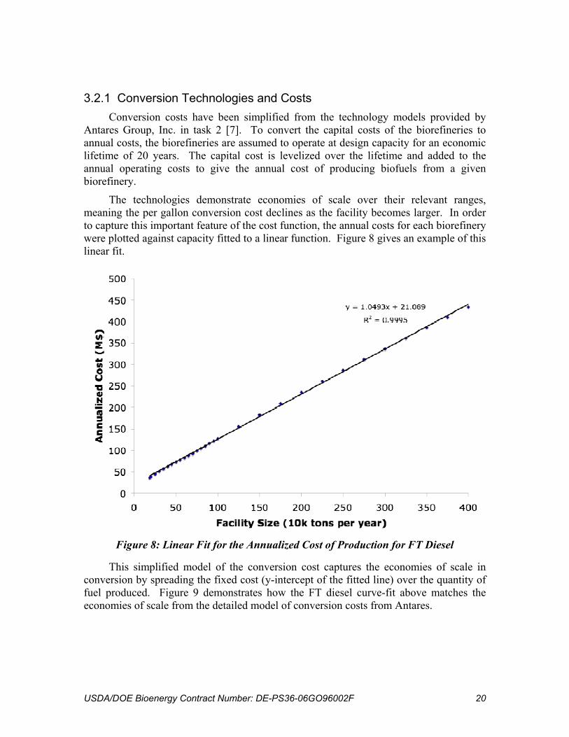
The technologies demonstrate economies of scale over their relevant ranges, meaning the per gallon conversion cost declines as the facility becomes larger. In order to capture this important feature of the cost function, the annual costs for each biorefinery were plotted against capacity fitted to a linear function. Figure 8 gives an example of this linear fit.
Figure 8: Linear Fit for the Annualized Cost of Production for FT Diesel
This simplified model of the conversion cost captures the economies of scale in conversion by spreading the fixed cost (y-intercept of the fitted line) over the quantity of fuel produced. Figure 9 demonstrates how the FT diesel curve-fit above matches the economies of scale from the detailed model of conversion costs from Antares.

USDA/DOE Bioenergy Contract Number: DE-PS36-06GO96002F 21
Figure 9: Linear fit to model estimate for economies of scale.
There are two biorefinery sizes that are important for determining the cost: feedstock input capacity and biofuel output capacity. The cost functions of each technology depend on either feedstock input or fuel product or both. The yield of fuel product per ton of feedstock input is not constant across feedstock types, which can lead to significantly different conversion costs by feedstock for technologies whose cost functions depend on input capacity.
The biorefineries are modeled to consume a constant mix of feedstock for the entire production period. The feedstock mix designates the conversion costs. This approach allows the biorefineries to take advantage of the resource mix in their area and not be constrained to a single feedstock type. Fuel campaigning to account for seasonality of production is not yet explicitly accounted for in the model.
Table 4 gives the values used for the cost functions in the model for each technology type. The maximum size constraint is given as the parameter M. The minimum facility size is not given in the model. Lower bounds of facility size are avoided due to the high unit cost incurred for small facilities caused by the fixed cost.

USDA/DOE Bioenergy Contract Number: DE-PS36-06GO96002F 22
Table 4: Annualized Conversion Costs for Biofuel Technologies Analyzed
Fixed Cost (million $)
Feed Dependent
($/ton)
Fuel Dependent ($/gallon)
Maximum Capacity
Model Parameter a b c M Grains to Ethanol:
Dry Mill Wet Mill
$2.17 $11.93
-
$0.32 $0.19
100 MGY 300 MGY
Lignocellulosic Ethanol $6.73 - $0.61 100 MGY Lignocellulosics to Middle Distillates
$21.11 $105 - 5 million tons
Lignocellulosics to Gasoline $2.13 $43.3 $0.46 800,000 tons Fatty Acids to Methyl Esters:
Yellow Grease Virgin oil/Tallow
$0.73 $1.66
$181 $62.3
-
320,000 tons 320,000 tons
Fatty Acids to Hydrocarbons $1.42 $44 - 800,000 tons
The conversion efficiency impacts the cost of biofuel production in two ways. First, lower conversion efficiencies require more production facility capital and operating cost per unit of fuel produced. Second, lower conversion efficiencies require more feedstock per of unit fuel produced. The conversion efficiencies for each biomass type/technology pair are given in Table 5.
Table 5: Assumed Conversion Efficiencies for Technologies by Biomass Type (gallons fuel / ton biomass)
Biomass Type GE LCE LCMD LCG1 FAME FAHC Corn Dry Mill 100
Wet Mill 89 - - - - -
Corn Stover - 80.6 36.8 21.6 - - Straws - 76.8 38.7 21.6 - - Orchard Vineyard Waste
- 76.9 40.6 22.0 - -
Forest - 90.2 42 22.0 - - MSW
-Mixed Paper -Wood Waste -Yard Waste -Mixed Waste
- - - -
86.0 78.9 70.0
-
37.1 41.5 38.4 31.6
23.2 22.0 21.6 21.6
- - - -
- - - -
Herbaceous Energy Crops
- 77.4 42.5 21.6 - -
Yellow Grease - - - - 249 250 Virgin Oils - - - - 260 250 Tallow and Lard - - - - 260 250
In the integrated supply curves we present the fuel supply in units of gallons of gasoline equivalent (gge), which is the number of gallons of gasoline that are displaced based on the energy in the fuels. We use this uniform metric of fuel energy to aggregate
1 Includes gasoline and diesel fuels.
USDA/DOE Bioenergy Contract Number: DE-PS36-06GO96002F 23
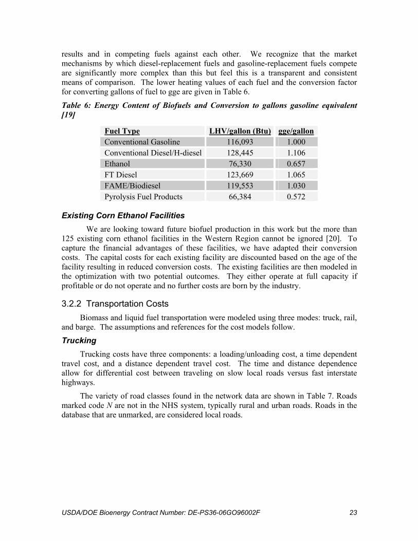
results and in competing fuels against each other. We recognize that the market mechanisms by which diesel-replacement fuels and gasoline-replacement fuels compete are significantly more complex than this but feel this is a transparent and consistent means of comparison. The lower heating values of each fuel and the conversion factor for converting gallons of fuel to gge are given in Table 6.
Table 6: Energy Content of Biofuels and Conversion to gallons gasoline equivalent [19]
Fuel Type LHV/gallon (Btu) gge/gallon Conventional Gasoline 116,093 1.000 Conventional Diesel/H-diesel 128,445 1.106 Ethanol 76,330 0.657 FT Diesel 123,669 1.065 FAME/Biodiesel 119,553 1.030 Pyrolysis Fuel Products 66,384 0.572
Existing Corn Ethanol Facilities We are looking toward future biofuel production in this work but the more than 125 existing corn ethanol facilities in the Western Region cannot be ignored [20]. To capture the financial advantages of these facilities, we have adapted their conversion costs. The capital costs for each existing facility are discounted based on the age of the facility resulting in reduced conversion costs. The existing facilities are then modeled in the optimization with two potential outcomes. They either operate at full capacity if profitable or do not operate and no further costs are born by the industry.
3.2.2 Transportation Costs Biomass and liquid fuel transportation were modeled using three modes: truck, rail,
and barge. The assumptions and references for the cost models follow.
Trucking Trucking costs have three components: a loading/unloading cost, a time dependent
travel cost, and a distance dependent travel cost. The time and distance dependence allow for differential cost between traveling on slow local roads versus fast interstate highways.
The variety of road classes found in the network data are shown in Table 7. Roads marked code N are not in the NHS system, typically rural and urban roads. Roads in the database that are unmarked, are considered local roads.

USDA/DOE Bioenergy Contract Number: DE-PS36-06GO96002F 24
Table 7: Road Travel Speed from NHPN
Code Route type Speed I Interstate 65 U US Route 65 S State Route 55 O Off-Interstate Business Marker 45 C County Route 45 T Township 35 M Municipal 35 P Parkway or Forest Route Marker 15 N Rural and Urban roads 35 {} local roads 25
The costs of biomass and fuel transport by truck are described in Table 8 [21-23]. Several important assumptions are embedded in these costs. The first is that trucking costs for all types of dry biomass feedstock are the same on a wet ton basis. Biomass transportation costs are only differentiated by their moisture content in defining payload (Table 9). The second is a $2.50 per gallon price of diesel. Finally, the cost of transporting all liquids (oils, grease, and fuel products) is considered to be the same on a volumetric basis.
Table 8: Trucking Costs
Liquids Bulk solids Comments Loading/unloading $0.02/gallon $5/wet ton
Time dependent $32/hr/truckload $29/hr/truckload Includes labor and capital Distance dependent $1.30/mile/truckload $1.20/mile/truckload Includes fuel, insurance,
maintenance, and permitting Truck Capacity 8,000 gallons 25 wet tons Moisture content varies with
feedstock
Table 9: Moisture Content of Biomass and Density of Liquid Feedstocks
Biomass type Moisture Content (% weight) Density (tons/1,000 gallons) Forest Wood Chips 50% - Straws (barley, oats, rye, wheat) 15% - Stover 15% - Orchard/Vineyard Waste 35% - Herbaceous Energy Crops 15% - Clean Mixed Paper (MSW) 10% - All Other MSW 50% - Corn 15% - Virgin Oil - 3.86
Yellow Grease - 3.24
Tallow/lard - 3.24

USDA/DOE Bioenergy Contract Number: DE-PS36-06GO96002F 25
Rail Rail costs here are based upon a mileage-based rate schedule for agricultural
products from Union Pacific railroad [24] . The costs are fitted to a linear model (Figure 10). These costs have a fixed component and a distance dependent component. We have also included a loading and unloading cost.
Table 10: Rail Transportation Costs
Liquid Bulk Solids Loading/unloading $0.015/gallon $5/wet ton Fixed Cost $8.80/100 gallons $27/wet ton Distance dependent $0.0075/mile/100 gallons $0.023/mile/wet ton Rail Car Capacity 33,000 gallons 106.5 wet tons
Published ethanol specific hauling rates show that the cost of a unit train with between 75 and 100 cars would lead to a 75-85% reduction in cost. This is not included in the cost functions used here.
Figure 10: Rate for Rail Transportation
Marine
Marine transportation costs are based on a published rate schedule for river barge [25]. The rates were fitted to a linear function of distance similar to the rail rates above.
USDA/DOE Bioenergy Contract Number: DE-PS36-06GO96002F 26
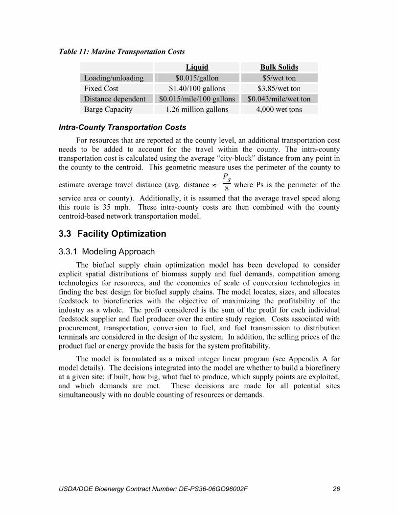
Table 11: Marine Transportation Costs
Liquid Bulk Solids Loading/unloading $0.015/gallon $5/wet ton Fixed Cost $1.40/100 gallons $3.85/wet ton Distance dependent $0.015/mile/100 gallons $0.043/mile/wet ton Barge Capacity 1.26 million gallons 4,000 wet tons
Intra-County Transportation Costs
For resources that are reported at the county level, an additional transportation cost needs to be added to account for the travel within the county. The intra-county transportation cost is calculated using the average “city-block” distance from any point in the county to the centroid. This geometric measure uses the perimeter of the county to
estimate average travel distance (avg. distance ≈ Ps8 where Ps is the perimeter of the
service area or county). Additionally, it is assumed that the average travel speed along this route is 35 mph. These intra-county costs are then combined with the county centroid-based network transportation model.
3.3 Facility Optimization
3.3.1 Modeling Approach The biofuel supply chain optimization model has been developed to consider
explicit spatial distributions of biomass supply and fuel demands, competition among technologies for resources, and the economies of scale of conversion technologies in finding the best design for biofuel supply chains. The model locates, sizes, and allocates feedstock to biorefineries with the objective of maximizing the profitability of the industry as a whole. The profit considered is the sum of the profit for each individual feedstock supplier and fuel producer over the entire study region. Costs associated with procurement, transportation, conversion to fuel, and fuel transmission to distribution terminals are considered in the design of the system. In addition, the selling prices of the product fuel or energy provide the basis for the system profitability.
The model is formulated as a mixed integer linear program (see Appendix A for model details). The decisions integrated into the model are whether to build a biorefinery at a given site; if built, how big, what fuel to produce, which supply points are exploited, and which demands are met. These decisions are made for all potential sites simultaneously with no double counting of resources or demands.

USDA/DOE Bioenergy Contract Number: DE-PS36-06GO96002F 27
Figure 11: Simplified Model Schematic
Models were developed for each of the three resource types – lignocellulosics, lipids and grains. In these models, the conversion technologies compete against each other for resources. For example, cellulosic ethanol, Fischer-Tropsch diesel and upgrading of pyrolysis oils to gasoline all compete for lignocellulosic resources.
Each model run gives results of the industry-wide fuel production for a given price; which biorefinery locations are optimal and how big they are; and which biomass resources are used by which biorefineries. Multiple model runs are performed over a range of fuel prices. Plotting the industry production against fuel price gives the supply curve for each resource type. The three supply curves for the three resource types are combined to produce the regional and state specific supply curves for biofuels.
3.3.2 Model Derivation and Solution Procedure The biorefinery siting optimization model is solved using the MIP solving
algorithm in CPLEX optimization software from ILOG using the GAMS model language [26]. The computational difficulty of the model depends on the number of variables with the number of binary variables being most important. Mixed integer solving algorithms will determine if a solution is optimal based on an optimality criterion that the objective is within a given percentage of the optimal solution for the “relaxed” linear formulation of the model. The more strict the optimality criteria the better the solution will be but the model becomes more computationally intensive with longer time needed to converge on the solution.
The flow chart below describes the structure of the model algorithm that is used for each resource type. The supply curves from the three resource types are subsequently combined in Excel by summing the three quantities at each price point.

USDA/DOE Bioenergy Contract Number: DE-PS36-06GO96002F 28
Figure 12: Supply Curve Generation
Initialize fuel selling price to minimum to be considered
Solve model
Save results
Price = maximum selling price?
Increment price: add (max-price – min_price)/n to the fuel price
Initialize model to produce n points along supply curve
with X% optimality criteria
Output results
Yes
No

USDA/DOE Bioenergy Contract Number: DE-PS36-06GO96002F 29
4 Results 4.1 Biomass Resources
There is a diverse biomass resource base in the WGA region that varies by the procurement cost and by location. Regionally, the resources that will be used by the biofuel industry will change as the price of biofuel increases. In the following two sections, we show the variation in feedstock supply by farm-gate, or procurement, cost and the spatial variation at various cost points.
4.1.1 Biomass Supply by Procurement Cost The available biomass supply will vary by the cost required to bring it to roadside
in a transportable form. A few of the types are available at set market prices or single cost but most have a range of availability over cost. Figures 13 and 14 show how the lignocellulosic and oil biomass resources vary with procurement cost. The corn resource has a maximum of 85.7 million dry tons available at $108.75 per ton ($3.05/bushel) constituting roughly 30% of the U.S. corn crop.
Figure 13: Lignocellulosic Biomass Resource Supply by Procurement Cost

USDA/DOE Bioenergy Contract Number: DE-PS36-06GO96002F 30
Figure 14: Oil Biomass Resource Supply by Procurement Cost
4.1.2 Biomass Resource Maps Resources are not uniformly distributed throughout the region. The maps below
show where the resources are located. The circles are municipal sources (MSW and waste grease) or point sources (oil seed pressing facilities). The scale is the same between the point sources and the county sources.

USDA/DOE Bioenergy Contract Number: DE-PS36-06GO96002F 31
Figure 15: Map of Corn Resources (no corn production associated with areas shaded
in green).

USDA/DOE Bioenergy Contract Number: DE-PS36-06GO96002F 32
Figure 16: Map of Lignocellulosic Feedstock Resources (no biomass production
associated with areas shaded in green).

USDA/DOE Bioenergy Contract Number: DE-PS36-06GO96002F 33
Figure 17: Map of Vegetable and Waste Oil Feedstock Resources

USDA/DOE Bioenergy Contract Number: DE-PS36-06GO96002F 34
4.2 Regional Biofuel Supply Curves The supply of biofuel over a range of fuel prices predicted by the model is shown
in Figure 18. For reference, 47.1 billion gallons of gasoline and 15.5 billion gallons of diesel fuel were sold in the WGA states in 2005 [27].
The supply curve represents the cost of producing the most expensive gallon of biofuel of the total quantity at the given price. In doing so, the curve shows the total quantity of fuel available under the price (marginal cost) because all gallons up to that point cost less than the price to produce and are therefore profitable to produce. This method is different from the method employed in the CDEAC bioenergy study in that the CDEAC study used the marginal producer to construct the supply [11]. The difference between the two methods is in the unit of analysis for constructing the supply curve. The advantage of the approach taken here is that it allows the system more flexibility to adjust to higher prices. For example, additional capacity can be added to a biorefinery to take advantage of higher prices even though it increases the biorefinery’scost of production.
For interpretation, it is important to note that the spatial distribution of demand and local fuel delivery are not included in the supply chain analysis. The local fuel delivery would likely add $0.20 to $0.35/gge in cost depending on the volumetric energy density of the fuel2. By not including the spatial distribution of demand in the analysis, we have ignored the potential need to transport biofuels significant distances to reach the appropriate fuel markets. This would further increase fuel cost.
2 Fuel distribution and marketing adds 20-22 cents per gallon for gasoline [28]. If the cost is the same on a volumetric basis, ethanol distribution and marketing would cost an additional 30-34 cents per gge.

USDA/DOE Bioenergy Contract Number: DE-PS36-06GO96002F 35
Figure 18: Regional Supply Curve for Biofuels
The supply of biofuels can be divided into gasoline-replacement fuels and diesel-replacement fuels by conversion technology. There are six conversion technologies used over the supply curve – wet and dry mill corn ethanol, lignocellulosic ethanol, FAME biodiesel, hydrotreatment of oils to diesel, and FT diesel. These technologies are deployed at different stages of the supply curve, with LCE coming on first and FT diesel deploying at only the highest prices. Corn ethanol has a very flat supply curve due to the commodity price of corn used in the model.
FAME biodiesel technology is deployed only at small scale and only over a limited range of diesel prices – from approximately $3/gge to $4/gge. This is the case of a couple of smaller oil seed resources that are far from a petroleum refinery. Fuel can be produced from them cheaper using small FAME biorefineries near the supply rather than transporting the resource to a large hydrotreatment facility co-located with a petroleum refinery. However, the FAME process is slightly less efficient than FAHC – producing 268 gge of fuel per ton of oils compared to 277 gge for the hydrotreatment process (FAHC). The result is that at very high fuel prices it is more profitable to produce a larger quantity of the more expensive fuel from a given resource. At this point the resource being used for FAME production is switched to FAHC production.

USDA/DOE Bioenergy Contract Number: DE-PS36-06GO96002F 36
Figure 19: Supply Curve for Gasoline-Replacement Biofuels
Figure 20: Supply Curve for Diesel-Replacement Biofuels
The biomass types that supply biofuel vary over the supply curve. Figure 21 shows which biomass types are being utilized at various cost points along the supply curve. The largest resources are corn, agricultural residues, herbaceous energy crops, MSW and

USDA/DOE Bioenergy Contract Number: DE-PS36-06GO96002F 37
forest resources. The jump in consumption for MSW resource near $4/gge is due to the deployment of the FT diesel technology consuming the mixed fraction of MSW. Note that introduction of sustainability standards and other sustainability conditions might significantly alter conclusions regarding corn and energy crop resources.
Figure 21: Biomass Supply at Biofuel Price by Type of Biomass
4.3 Target Price Results
4.3.1 Target Price A target price is used in conjunction with the supply curves to evaluate the
quantity of biofuels that will be available in the year 2015. In keeping with the CDEAC biopower assessment, the target price is set 38% above the projected wholesale gasoline and diesel prices for 2015. The wholesale price is used to match the end point of the modeling analysis at the nearest distribution terminal. There will be some difference in the local fuel distribution costs due to differences in volumetric energy densities of the fuels, which is not captured here. The difference between the fuel market price and the target can be reduced or eliminated through state, regional or federal policies. The target price is based on the energy content of the fuel and is $2.40 per gasoline gallon equivalent (gge) for gasoline replacement fuels and $2.36 per gge for diesel replacement fuels.

USDA/DOE Bioenergy Contract Number: DE-PS36-06GO96002F 38
4.3.2 Mapping Biofuel Industry in Western United States at Target Price The biofuel industry that results at the target price is illustrated in Figure 22. The
majority of the biorefineries are located either near large municipal sources of waste feedstock or in agricultural areas.
Figure 22: Map of biofuels production in the Western Governors Association region
for a target fuel price of $2.40/gge.
4.3.3 Supply Maps by State Biofuel supply maps that show the quantity of biofuel that can be produced at the
target price for each state have been developed. A complete map atlas of all the western states can be found in Appendix B. The maps display the transportation infrastructure, optimized biorefinery locations with production levels, feedstock density, and distribution terminals. The maps are coupled with state specific supply curves for biofuels production. The biofuel production in each state and from state resources are aggregated into state-specific supply curves for each state.

USDA/DOE Bioenergy Contract Number: DE-PS36-06GO96002F 39
Figure 23: Map of biofuels production in Kansas for a target price of $2.40/gge. (see
appendix for map legend)
USDA/DOE Bioenergy Contract Number: DE-PS36-06GO96002F 40
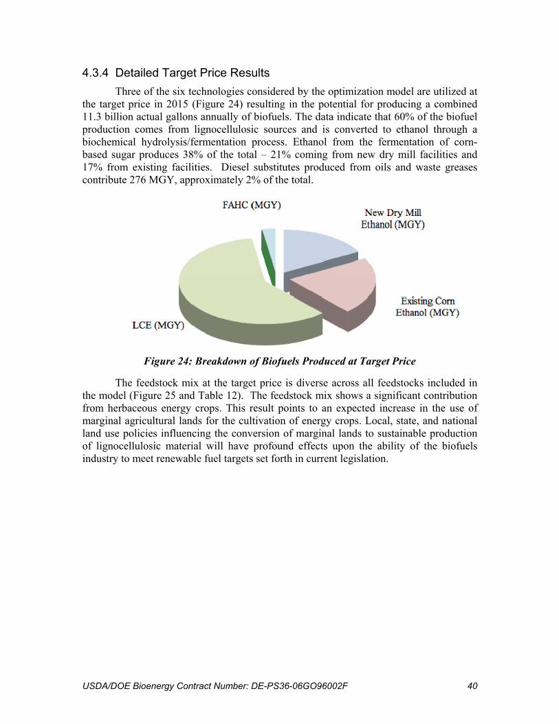
4.3.4 Detailed Target Price Results Three of the six technologies considered by the optimization model are utilized at
the target price in 2015 (Figure 24) resulting in the potential for producing a combined 11.3 billion actual gallons annually of biofuels. The data indicate that 60% of the biofuel production comes from lignocellulosic sources and is converted to ethanol through a biochemical hydrolysis/fermentation process. Ethanol from the fermentation of corn-based sugar produces 38% of the total – 21% coming from new dry mill facilities and 17% from existing facilities. Diesel substitutes produced from oils and waste greases contribute 276 MGY, approximately 2% of the total.
Figure 24: Breakdown of Biofuels Produced at Target Price
The feedstock mix at the target price is diverse across all feedstocks included in the model (Figure 25 and Table 12). The feedstock mix shows a significant contribution from herbaceous energy crops. This result points to an expected increase in the use of marginal agricultural lands for the cultivation of energy crops. Local, state, and national land use policies influencing the conversion of marginal lands to sustainable production of lignocellulosic material will have profound effects upon the ability of the biofuels industry to meet renewable fuel targets set forth in current legislation.

USDA/DOE Bioenergy Contract Number: DE-PS36-06GO96002F 41
Figure 25: Feedstock Consumption at Target Price
Table 12: Feedstock Consumed in Target Price Configuration
Feedstock Feedstock consumption at $2.40/gge (million tons) Corn 43.9 Forest biomass 11.2 Waste grease 0.2 Herbaceous energy crops 43.1 Municipal solid waste 19 Orchard and vineyard waste 2.9 Corn Stover 0.8 Straw (wheat, barley, rye, oats) 7.9 Tallow 0.9
Total 130
The cost of production of biofuels within the model can be broken into four distinct components.
• Feedstock costs, paid to the farmer at the farm gate or operator at point of origin.
• Transportation costs, incurred in transporting feedstock from source to biorefinery.
• Conversion costs, amortized costs of converting feedstock into fuel.
• Distribution costs, costs associated with the transport of fuel from the biorefinery to the distribution terminal.

USDA/DOE Bioenergy Contract Number: DE-PS36-06GO96002F 42
Figure 26: Breakdown of Costs for Biofuels Produced
The cost breakdown varied significantly among the conversion technologies. Corn-based ethanol and diesel replacement production costs are heavily weighted toward procurement costs resulting from the high cost of corn, greases and tallows. In contrast, cellulosic ethanol production costs are more evenly distributed among the procurement, transport, and conversion costs. The higher costs of transport and conversion are a result of the low bulk density of cellulosic materials and the early stage of development for commercial cellulosic conversion technologies.
The farm gate prices paid for feedstocks also vary significantly. This variability in farm gate prices generally reflects the presence or absence of existing markets for feedstock. The market effects of the growth in demand for current low- or negative-value biomass, such as municipal solid waste, is not incorporated into this model and should be considered in future analysis. Also, the projected modeled costs of dedicated energy crops are, as yet, highly speculative and will certainly be affected by increases in demand created by new capacity for cellulosic ethanol production.

USDA/DOE Bioenergy Contract Number: DE-PS36-06GO96002F 43
Figure 27: Procurement Cost for Lignocellulosic Resources used in Target Price
Configuration
4.4 Sensitivity Analysis
Seven sensitivity analyses were performed; five resource sensitivities and two technology sensitivities.
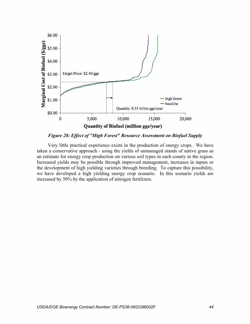
There is large uncertainty associated with the resource assessments. Two forest resource assessments were performed by Ken Skog et al [8], of the US Forest Service, to capture the uncertainty in forest-based biomass supply. In addition to the baseline, a “high forest” case assessment was performed. The result of switching to a “high forest” case in the integrated supply curve is an increase of 850 million gge per year in biofuel production at the $2.40/gge and an even greater increase of 1,500 million gge per year at $3.00/gge.
USDA/DOE Bioenergy Contract Number: DE-PS36-06GO96002F 44
Figure 28: Effect of "High Forest" Resource Assessment on Biofuel Supply
Very little practical experience exists in the production of energy crops. We have taken a conservative approach - using the yields of unmanaged stands of native grass as an estimate for energy crop production on various soil types in each county in the region. Increased yields may be possible through improved management, increases in inputs or the development of high yielding varieties through breeding. To capture this possibility, we have developed a high yielding energy crop scenario. In this scenario yields are increased by 50% by the application of nitrogen fertilizers.
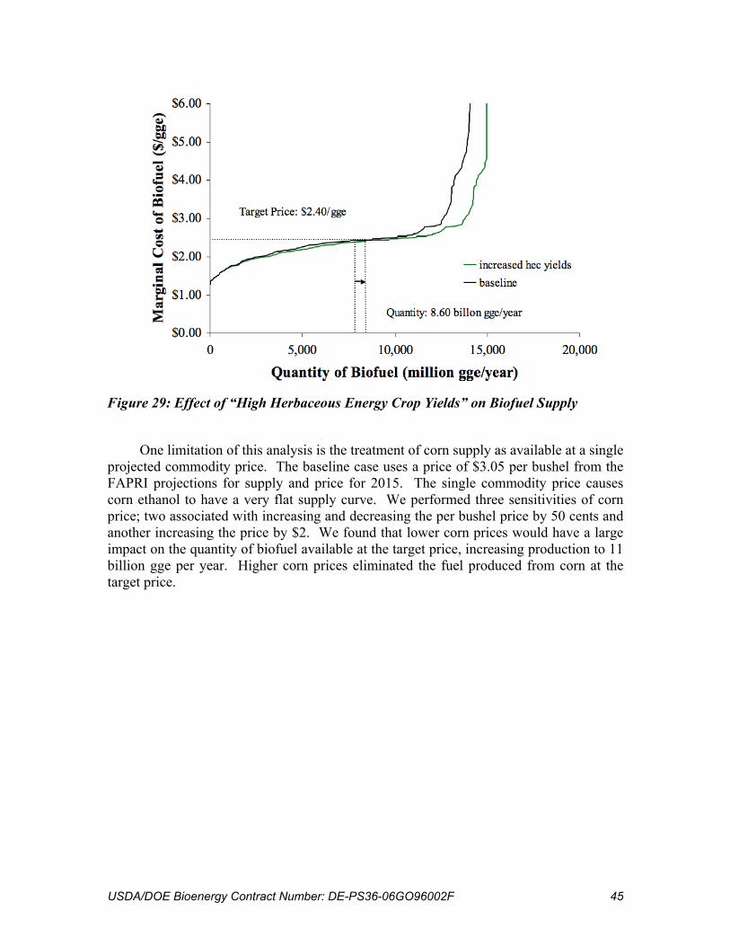
USDA/DOE Bioenergy Contract Number: DE-PS36-06GO96002F 45
Figure 29: Effect of “High Herbaceous Energy Crop Yields” on Biofuel Supply
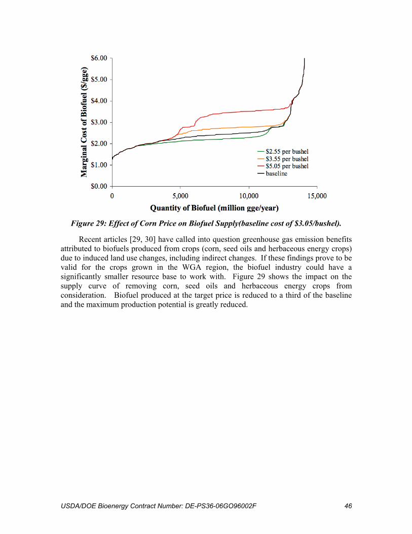
One limitation of this analysis is the treatment of corn supply as available at a single projected commodity price. The baseline case uses a price of $3.05 per bushel from the FAPRI projections for supply and price for 2015. The single commodity price causes corn ethanol to have a very flat supply curve. We performed three sensitivities of corn price; two associated with increasing and decreasing the per bushel price by 50 cents and another increasing the price by $2. We found that lower corn prices would have a large impact on the quantity of biofuel available at the target price, increasing production to 11 billion gge per year. Higher corn prices eliminated the fuel produced from corn at the target price.
USDA/DOE Bioenergy Contract Number: DE-PS36-06GO96002F 46
Figure 29: Effect of Corn Price on Biofuel Supply(baseline cost of $3.05/bushel).
Recent articles [29, 30] have called into question greenhouse gas emission benefits attributed to biofuels produced from crops (corn, seed oils and herbaceous energy crops) due to induced land use changes, including indirect changes. If these findings prove to be valid for the crops grown in the WGA region, the biofuel industry could have a significantly smaller resource base to work with. Figure 29 shows the impact on the supply curve of removing corn, seed oils and herbaceous energy crops from consideration. Biofuel produced at the target price is reduced to a third of the baseline and the maximum production potential is greatly reduced.

USDA/DOE Bioenergy Contract Number: DE-PS36-06GO96002F 47
Figure 30: Effect of Excluding Corn, Oil Seeds and Herbaceous Energy Crops on
Biofuel Supply
The development of a biofuel technology that meets the projected performance of lignocellulosic ethanol technologies in this analysis is important to achieving the supply at prices shown in the results. To bound the impact of this technology improvement, we have performed a scenario of stalled technology where the lignocellulosic ethanol technology only achieves the near-term performance described in the Task 2 report [7]. This includes significantly higher conversion costs and lower yields. At this lower level of performance the supply of biofuels is significantly reduced at the target price (22% of baseline). From another perspective, it will take 28 cents per gge more to induce the same quantity of fuel production at the same technology status. This represents a shift from lignocellulosic resource use to a larger reliance on corn-based ethanol.

USDA/DOE Bioenergy Contract Number: DE-PS36-06GO96002F 48
Figure 31: Effect of Stalled LCE Technology on Biofuel Supply
By building larger biorefineries, the fixed costs can be spread over a larger quantity of fuel produced. In this analysis, we account for these economies of scale but we place a cap on the size of the biorefinery. It is uncertain at this time what the maximum size of these facilities will be. We performed a sensitivity by increasing the maximum capacity of the LCE biorefineries from 100 MGY to 200 MGY while holding the per unit cost of conversion constant beyond 100 MGY. This resulted in only small cost savings at the low end of the supply curve.

USDA/DOE Bioenergy Contract Number: DE-PS36-06GO96002F 49
Figure 32: Effect of Maximum LCE Biorefinery Size on Supply Curve
USDA/DOE Bioenergy Contract Number: DE-PS36-06GO96002F 50
5 Discussion The model results illustrate the potential to produce substantial quantities of biofuels
from western U.S. biomass resources, but they are also subject to substantial uncertainties. In interpreting the supply estimates, unresolved questions remain regarding economic performance of the different conversion technologies and the overall sustainability of many of the biomass resources considered. 5.1 Important Factors Determining Supply
The biofuel supply in the western states relies on a diverse resource base with significant contributions from multiple resources. The key determinants of supply vary across the states in the region. The region-wide supply is most sensitive to the following factors.
• The development of low-cost cellulosic ethanol technology or a technology with similar performance to LCE as modeled,
• The availability and yield of herbaceous energy crops from marginal farmland,
• The price and availability of corn for fuel production,
• Acceptability of MSW resources as a biofuel feedstock,
• Access to forest resources.
Each of these factors is under active research and estimates can be refined as new information becomes available. The sensitivity analyses provide some sense of how resource and fuel supplies might shift under relevant future scenarios. Further, this analysis is independent of resource competition from other energy and bio-based product uses, including electricity and heat applications. Integrated biorefineries involving poly-generation of multiple energy products may resolve some uncertainty in this regard, but more detailed models explicitly including these alternate markets will need to be explored to examine biofuel supply effects. Over the longer term, changes in transportation system design, for example, to include more electric or hybrid-electric vehicles, and improvements in energy use efficiency will also shift energy demand, as will regulatory and policy influences, such as imposition of carbon or fuel taxes and introduction of low-carbon fuel standards requiring LCA certification. Model refinement to incorporate more detailed sustainability and econometric considerations along with seasonal and stochastic effects will be needed to reduce supply uncertainties. 5.2 Relevance to Existing Policies
The model application to the assumptions for 2015 results in a biofuel supply in the WGA states of 11.3 billion actual gallons per year (not adjusted to gge) at the $2.40/gge target price.
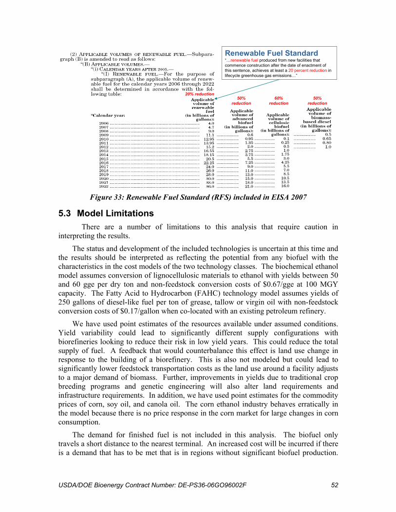
The federal Energy Independence and Security Act (EISA) of 2007 includes a renewable fuel standard (RFS) scheduling annual renewable fuel supplies to achieve 36 billion actual gallons by 2022. For the time frame modeled here, EISA requires 20.5
USDA/DOE Bioenergy Contract Number: DE-PS36-06GO96002F 51
billion gallons of renewable fuel by 2015, of which 5.5 billion gallons are from advanced biofuels and 3.0 billion gallons are from cellulosic biofuels (Figure 33). EISA specifies that by 2012, 1 billion gallons of biomass-based diesel fuel will be available. EISA also includes specific reductions in life-cycle greenhouse gas (GHG) emissions to accompany the various fuel types. Advanced biofuels and biomass-based diesel fuels must achieve a 50% reduction over baseline gasoline GHG emissions, while cellulosic biofuels must achieve a 60% reduction. The remaining renewable fuel, such as from corn, need only achieve a 20% reduction.
The WGA states can have an important role in helping to meet national RFS objectives. At the base fuel target price, the 11.3 billion gallons of biofuel projected by the model is 55% of the national standard in that year. Below $3/gge, biomass-based diesel fuel supplies from the west would likely be only about a quarter of the EISA 2012 standard, whereas western cellulosic supplies for the same price range would be sufficient to meet about 70% of the EISA standard of 7.25 billion gallons in 2016. These amounts are at present highly speculative, especially considering that not all biomass will be used for biofuels in competition with other energy markets.
The extent to which the west could sustain such shares in meeting the 2022 RFS amounts has not been specifically modeled. If biofuel production were not further increased, the 55% share at the base target price for 2015 would erode to less than a third of national supply in 2022, although this share would still constitute a substantial economic opportunity. Certifying GHG reductions consistent with the EISA requirements will be an important task for future development.
USDA/DOE Bioenergy Contract Number: DE-PS36-06GO96002F 52
Renewable Fuel Standard“…renewable fuel produced from new facilities that commence construction after the date of enactment of this sentence, achieves at least a 20 percent reduction in lifecycle greenhouse gas emissions…”
50% reduction
60% reduction
50% reduction
20% reduction
Figure 33: Renewable Fuel Standard (RFS) included in EISA 2007
5.3 Model Limitations There are a number of limitations to this analysis that require caution in
interpreting the results.
The status and development of the included technologies is uncertain at this time and the results should be interpreted as reflecting the potential from any biofuel with the characteristics in the cost models of the two technology classes. The biochemical ethanol model assumes conversion of lignocellulosic materials to ethanol with yields between 50 and 60 gge per dry ton and non-feedstock conversion costs of $0.67/gge at 100 MGY capacity. The Fatty Acid to Hydrocarbon (FAHC) technology model assumes yields of 250 gallons of diesel-like fuel per ton of grease, tallow or virgin oil with non-feedstock conversion costs of $0.17/gallon when co-located with an existing petroleum refinery.
We have used point estimates of the resources available under assumed conditions. Yield variability could lead to significantly different supply configurations with biorefineries looking to reduce their risk in low yield years. This could reduce the total supply of fuel. A feedback that would counterbalance this effect is land use change in response to the building of a biorefinery. This is also not modeled but could lead to significantly lower feedstock transportation costs as the land use around a facility adjusts to a major demand of biomass. Further, improvements in yields due to traditional crop breeding programs and genetic engineering will also alter land requirements and infrastructure requirements. In addition, we have used point estimates for the commodity prices of corn, soy oil, and canola oil. The corn ethanol industry behaves erratically in the model because there is no price response in the corn market for large changes in corn consumption.
The demand for finished fuel is not included in this analysis. The biofuel only travels a short distance to the nearest terminal. An increased cost will be incurred if there is a demand that has to be met that is in regions without significant biofuel production.

USDA/DOE Bioenergy Contract Number: DE-PS36-06GO96002F 53
The pull of large population centers to import fuels from agricultural areas will change the configuration of the supply chain and hence fuel cost into final demand.
The spatial arrangement of the biofuels supply chain as modeled here should be considered with the following caveats. The allocation of feedstock supply sources to biorefinery sites for feedstocks attributed to counties may not accurately reflect the least cost transport route to a biorefinery. This is the result of the spatial scale of the county-level feedstock source and artificial boundary constraints exemplified by the eastern edge of the WGA territory. Further, the model at present ignores imports of both biomass feedstock and finished biofuels from outside the region. Feedstock sources were located at the geographic center of the county. Thus the variability in distribution of feedstock throughout the county is overlooked. As a result, in counties where there is a great deal of variability in feedstock density, it may be more economical to connect feedstock sources within a county to multiple biorefineries. This limitation is an artifact of the objectives influencing the design of the model. The primary objective in formulating the model was to generate a region-wide supply curve. With this purpose in mind, the variability in transport cost that the current model formulation overlooks is acceptable. A logical extension of this model would be to enable the analysis of feedstock profile and availability for the purposes of facility siting and feasibility analysis. This model can provide crude results for such an analysis but to provide more rigorous results for site feasibility analysis, the incorporation of higher resolution feedstock mapping would be a critical component.

USDA/DOE Bioenergy Contract Number: DE-PS36-06GO96002F 54
6 Conclusions This modeling effort contributes greatly to an understanding of the feasibility,
constraints, and potential for the expansion of a biofuels industry in the western U. S. Recent legislation at the federal and state levels mandating timelines for offsetting fossil fuel use in transportation by renewable and low-carbon fuels, as well as legislation constraining the emission of greenhouse gases from the transportation and other sectors necessitates the development of realistic data and models to assess technical feasibility of meeting these goals. This model, even if preliminary, constitutes a comprehensive framework for spatially explicit integrated analysis of the entire biofuel supply chain. As any model its foremost limitation is in the quality of the input data. The results of this modeling effort indicate that there is significant potential to expand biofuels production in the west. This model should be used to model the effects of policy and market scenarios related to biofuels production, and extended across the nation to eliminate arbitrary boundary effects, a revision currently in progress. Exclusive of resource competition from other energy and product markets, there is the potential for the west to supply substantial fractions of renewable fuels under the new federal RFS. Additional conclusions concerning major land use and transportation infrastructure among other effects include the following:
Land Use:
• Land use policies will have a significant impact on the availability feedstock.
• Land use policies should enable the expansion of herbaceous energy crop production on marginal lands, but must be based on substantive sustainability standards or research findings.
• Land use policy formulation should carefully explore the possibility of meeting GHG reduction targets under the federal RFS through more sustainable energy crop substitution on lands currently producing corn and other high-input crops at low relative yields.
Transportation:
• A more detailed analysis is needed of the capacity of existing transportation infrastructure to meet demands of the biofuel supply chain.
• A spatially explicit analysis should be conducted of the potential for new transportation infrastructure to improve supply chain economics for biofuels production.

USDA/DOE Bioenergy Contract Number: DE-PS36-06GO96002F 55
7 References 1. Perlack, R.D., et al., Biomass as Feedstock for a Bioenergy and Bioproducts Industry: The Technical Feasibility of a Billion-Ton Annual Supply, 2005, Oak Ridge, TN, http://feedstockreview.ornl.gov/pdf/billion_ton_vision.pdf.
2. Walsh, M., et al. Biomass Feedstock Availability in the United States: 1999 State Level Analysis. 1999 January, 2000 [cited Febuary 22, 2007]; Available from: http://bioenergy.ornl.gov/resourcedata/index.html.
3. Graham, R.L., B.C. English, and C.E. Noon, A Geographic Information System-based modeling system for evaluating the cost of delivered energy crop feedstock. Biomass and Bioenergy, 2000. 18(4): p. 309-329.
4. Kaylen, M., et al., Economic feasibility of producing ethanol from lignocellulosic feedstocks. Bioresource Technology, 2000. 72(1): p. 19-32.
5. Freppaz, D., et al., Optimizing forest biomass exploitation for energy supply at a regional level. Biomass and Bioenergy, 2004. 26(1): p. 15-25.
6. Parker, N., Optimizing the Design of Biomass Hydrogen Supply Chains Using Real-World Spatial Distributions: A Case Study Using California Rice Straw, in Transportation Technology and Policy. 2007, University of California, Davis: Davis, CA
7. Antares Group Inc, Strategic Development of Bioenergy in the Western States: Development of Supply Scenarios Linked to Policy Recommendations; Section 2: Bioenergy Conversion Technology Characteristcs. 2008, Western Governors' Association
8. Nelson, R., K. Skog, and R. Rummer, Strategic Development of Bioenergy in the Western States: Development of Supply Scenarios Linked to Policy Recommendations; Section 1: Biomass Resource Assessment and Supply Analysis for the WGA Region. 2008, Western Govenors' Association.
9. McCoy, J., Using ArcGIS Spatial Analyst, 2005, http://support.esri.com/index.cfm?fa=knowledgebase.documentation.listDocs&PID=47.
10. The PostgreSQL Global Development Group, PostgreSQL 8.1.4 Documentation, 2005.
11. Western Governors' Association (WGA), Clean and Diversified Energy Initiative: Biomass Task Force Report, 2006, http://www.westgov.org/wga/initiatives/cdeac/biomass.htm.
12. Environmental Protection Agency (EPA), EnviroFacts Facility Registration System. 2007.
13. National Atlas of the United States, Cities and Towns of the United States, 2004, Reston, VA, http://nationalatlas.gov/atlasftp.html.
14. OPISnet.com, Petroleum Terminal Encyclopedia. 2007.
15. Federal Highway Administration (FHWA), National Highway Planning Network, 2005, Washington, DC, http://www.fhwa.dot.gov/.

USDA/DOE Bioenergy Contract Number: DE-PS36-06GO96002F 56
16. Federal Railroad Administration (FRA), Rail Lines, 2007, Washington, DC, http://www.bts.gov/programs/geographic_information_services/.
17. Research and Innovative Technology Administration's Bureau of Transportation Statistics (RITA/BTS), Facilities, 2003, Washington, DC, http://www.bts.gov/programs/geographic_information_services/.
18. Research and Innovative Technology Administration’s Bureau of Transportation Statistics (RITA/BTS), US Army Corps of Engineers Ports, 2006, Alexandria, VA, http://www.bts.gov/programs/geographic_information_services/.
19. Unnasch, S. and J. Pont, Fuel Cycle Assessment: Well-To-Tank Energy Inputs, Emissions and Water Impacts - DRAFT CONSULTANT REPORT, 2007, http://www.energy.ca.gov/2007publications/CEC-600-2007-002/CEC-600-2007-002-D.PDF.
20. Antares Group Inc, U.S. Ethanol Facilities. 2007.
21. Jenkins, B.M., et al., Equipment Performances, Costs, and Constraints in the Commercial Harvesting of Rice Straw for Industrial Applications, in 2000 ASAE Annual International Meeting. 2000: Milwaukee, WI.
22. Perlack, R.D. and A.F. Turhollow, Feedstock cost analysis of corn stover residues for further processing. Energy, 2003. 28(14): p. 1395-1403.
23. Reynolds, R., Infrastructure Requirements for an Expanded Fuel Ethanol Industry, Oak Ridge National Laboratory and Department of Energy, Editors. 2002.
24. Union Pacific Railroad. Item 1000-AG Mileage Scale. 2007 [cited.
25. Tidewater. Rate Schedule 200-A. 2007 [cited; Available from: http://www.tidewater.com/transport.php.
26. McCarl, B.A., GAMS User Guide. GAMS Development Corporation, 2004.
27. Energy Information Administration (EIA), State Energy Consumption, Price, and Expenditure Estimates (SEDS), 2008, Washington, DC, http://www.eia.doe.gov/emeu/states/_seds.html.
28. Energy Information Administration (EIA), A Primer on Gasoline Prices, 2006, Washington, DC.
29. Fargione, J., et al., Land Clearing and the Biofuel Carbon Debt. Science, 2008. 319(5867): p. 1235-1238.
30. Searchinger, T., et al., Use of U.S. Croplands for Biofuels Increases Greenhouse Gases Through Emissions from Land-Use Change. Science, 2008. 319(5867): p. 1238-1240.

USDA/DOE Bioenergy Contract Number: DE-PS36-06GO96002F 57
8 Appendices 8.1 Appendix A: Details of Supply Chain Optimization Model Objective Function for Optimization
The optimization model is a mixed integer-linear program with the objective to maximize the total annual profit of producing and delivering biofuels to a distribution terminal. The profit is defined here as the annual revenue from the sale of biofuels less the annual cost of producing those biofuels. The annual profit equation is as follows:
Profit = fuel_ price ⋅ gget ⋅Ybjt − Costjt
∑ (1)
where
Cost = PCifp + DCijf( )⋅ Fijfp{ }+ at ⋅ X jt + bt ⋅Yf fjt
f
∑ + ct ⋅Ybjt
jt
∑ + TC jt ⋅Ybjt
jt
∑ijfp
∑ (2)
The subscripts ‘i’ and ‘j’ correspond locations of biomass supply points and potential biorefineries, respectively. The subscript ‘f’ denotes the type of biomass feedstock, the subscript ‘t’ denotes the conversion technology and the subscript ‘p’ represents a procurement price level. The important variables are parameters are listed in Table 12.
Table 12: Meaning model variables and parameters
Variable Definition Fijfp Yearly quantity of biomass of type ‘f’ at price level ‘p’ delivered from
source ‘i’ to biorefinery ‘j’ Xjt Binary variable that is 0 if no biorefinery using technology ‘t’ exist at site
‘j’ and 1 if a biorefinery is built at site ‘j’ Yffjt Size of the biorefinery using technology ‘t’ at site ‘j’ in terms of biomass
input differentiated by type of biomass Ybjt Size of the biorefinery using technology ‘t’ at site ‘j’ in terms of biofuel
output Parameters
fuel_price Selling price of product biofuel PCifp Procurement cost for biomass of type ‘f’ from source ‘i’ at price level ‘p’ DCijf Delivery cost for biomass of type ‘f’ from source ‘i’ to biorefinery site ‘j’ at Fixed conversion cost for biorefinery using technology ‘t’ bt Variable conversion cost that scales with biomass input ct Variable conversion cost that scales with biofuel output TCj Cost of delivery of a unit of fuel from biorefinery site ‘j’ to the nearest
distribution terminal Supplyifp Quantity of biomass of type ‘f’ available at source ‘i’ for price level ‘p’ ηft Conversion efficiency for biomass of type ‘f’ using technology ‘t’ M Maximum size of biorefinery in units of biomass input
USDA/DOE Bioenergy Contract Number: DE-PS36-06GO96002F 58
Constraints
The objective function is combined with a number of constraints representing the physical limitations or restrictions of the biomass industry in the mathematical model. Supply Constraints
The first set of constraints limits the biomass originating from a source at a price level to be less than the maximum supply of biomass of that type at that price level at that source.
ifpj
ijfp SupplyF ≤∑ (3)
Conservation of mass at biorefinery
The biofuel produced at a biorefinery is equal to the quantity of biofuel that can be produced from the biomass entering the biorefinery given the conversion efficiency including handling loss. We also relate the biorefinery’s biomass input capacity to the biomass coming into the facility.
∑∑ =t
fjtip
ijfp YfF (4)
∑ ⋅=ft
fjtftjt YfYb η (5)
Fixed cost constraint
There can be no biorefinery size if the fixed cost has not been paid (binary variable at that site is 0). If the binary variable is 1 then the biorefinery can be no greater than its maximum size from the engineering cost equations.
jtf
fjt XMYf ⋅≤∑ (6)
Non-negativity
All variables representing physical quantities must take on either a zero or positive value.
Fijfp ,Yf fjt,Ybjt ≥ 0 (7)

USDA/DOE Bioenergy Contract Number: DE-PS36-06GO96002F 59
8.2 Appendix B: State Atlas State supply curves and maps are shown for biofuels produced from the biomass resources of the state and the predicted in-state fuel production. The range of in state production results from border effects where biorefineries are nearly as likely to be located in one state as it is to be located in a neighboring state. Some states are predicted to be net importers or exporters of biomass feedstock. In many cases this is due to potential biorefinery sites being chosen near a state border and reflects which border towns have larger populations. In a few cases, the resource basins include a small fraction of one state but are centered in another. In these cases, the effect is a robust result.
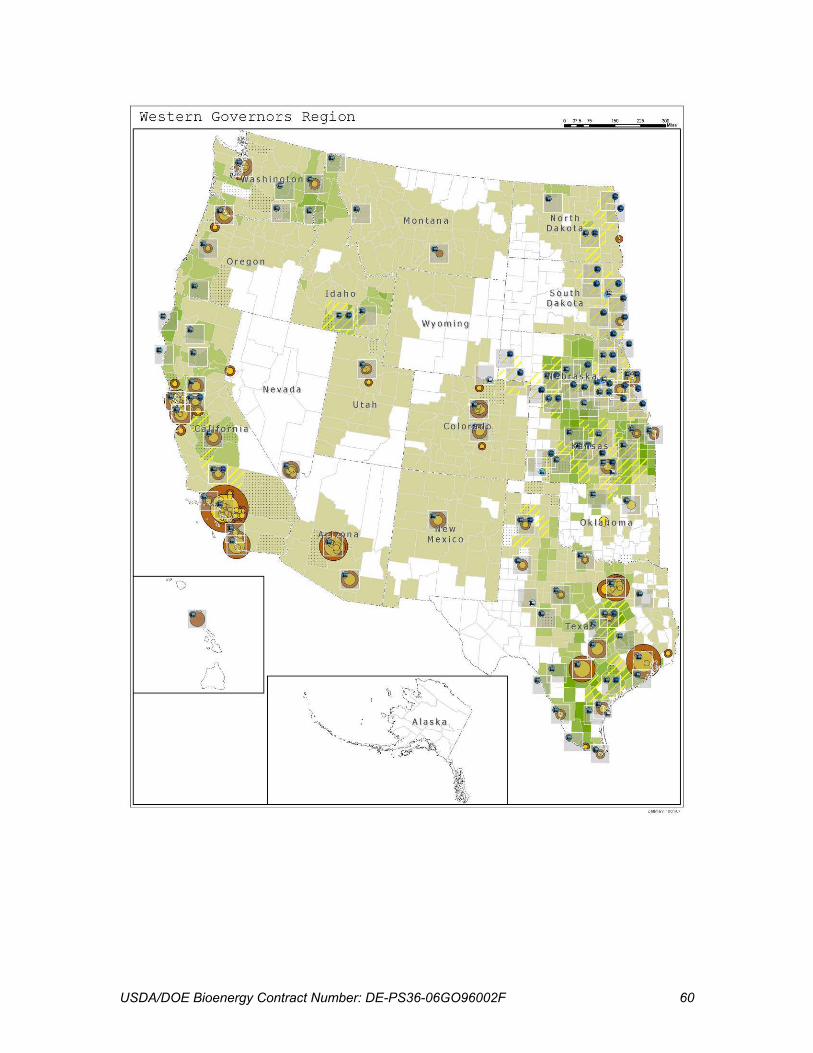
USDA/DOE Bioenergy Contract Number: DE-PS36-06GO96002F 60

USDA/DOE Bioenergy Contract Number: DE-PS36-06GO96002F 61

USDA/DOE Bioenergy Contract Number: DE-PS36-06GO96002F 62

USDA/DOE Bioenergy Contract Number: DE-PS36-06GO96002F 63
ARIZONA SUPPLY CURVES Figure 34: Production of biofuels in Arizona and from Arizona's resources
Figure 35: Consumption of Arizona's biomass resources for biofuel production
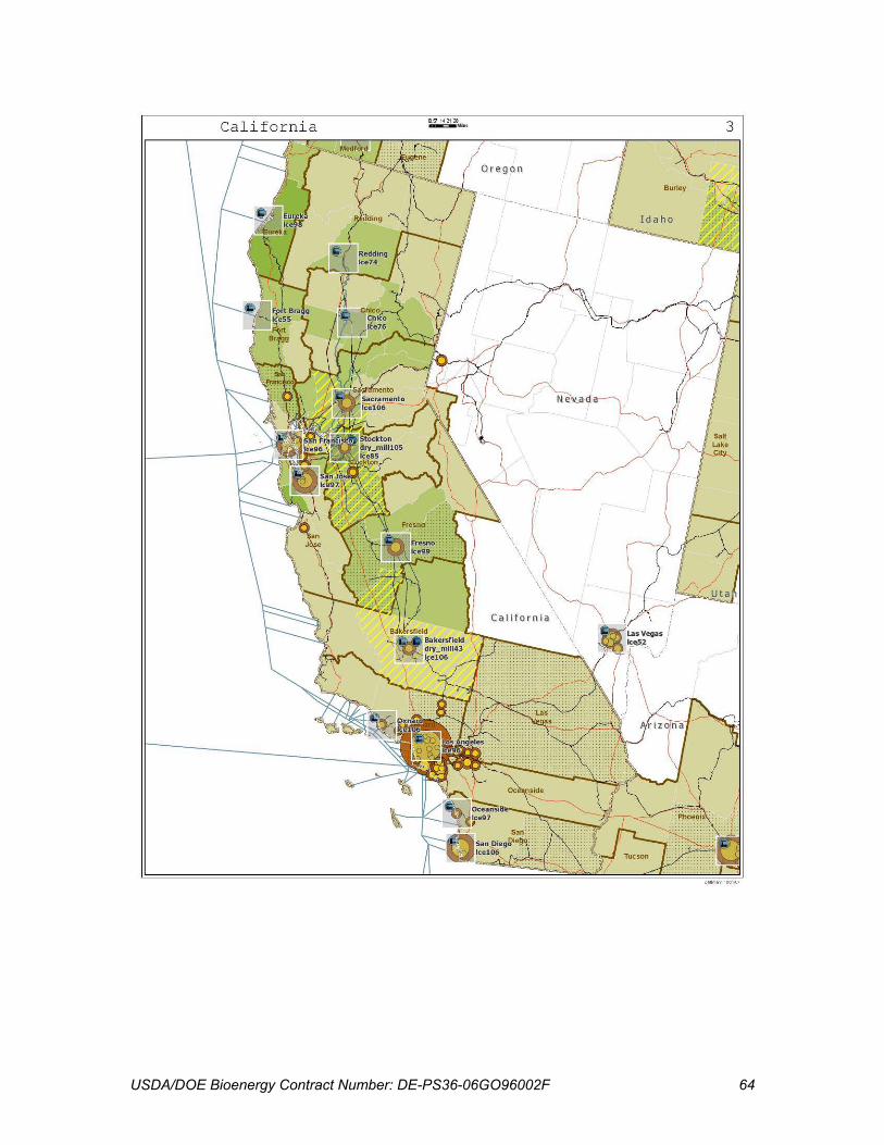
USDA/DOE Bioenergy Contract Number: DE-PS36-06GO96002F 64

USDA/DOE Bioenergy Contract Number: DE-PS36-06GO96002F 65
CALIFORNIA SUPPLY CURVES Figure 36: Production of biofuels in California and from California's resources
Figure 37: Consumption of California’s biomass resources for biofuel production

USDA/DOE Bioenergy Contract Number: DE-PS36-06GO96002F 66

USDA/DOE Bioenergy Contract Number: DE-PS36-06GO96002F 67
COLORADO SUPPLY CURVES Figure 38: Production of biofuels in Colorado and from Colorado's resources
Figure 39: Consumption of Colorado’s biomass resources for biofuel production

USDA/DOE Bioenergy Contract Number: DE-PS36-06GO96002F 68
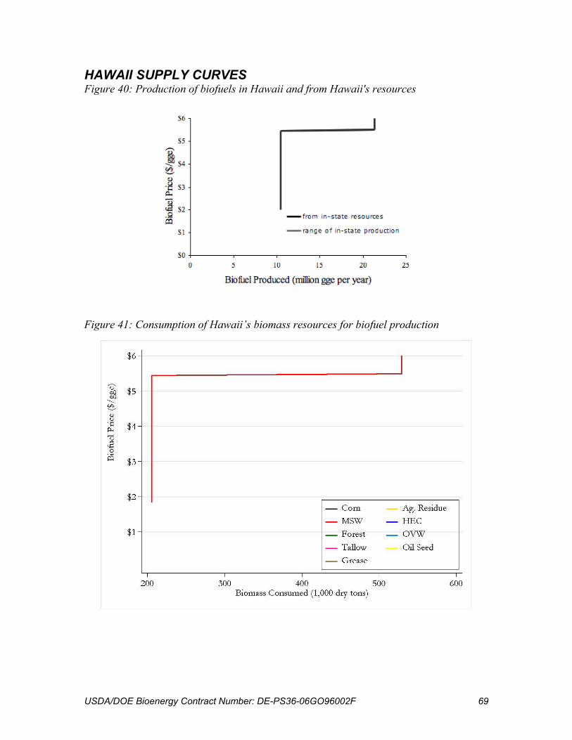
USDA/DOE Bioenergy Contract Number: DE-PS36-06GO96002F 69
HAWAII SUPPLY CURVES Figure 40: Production of biofuels in Hawaii and from Hawaii's resources
Figure 41: Consumption of Hawaii’s biomass resources for biofuel production
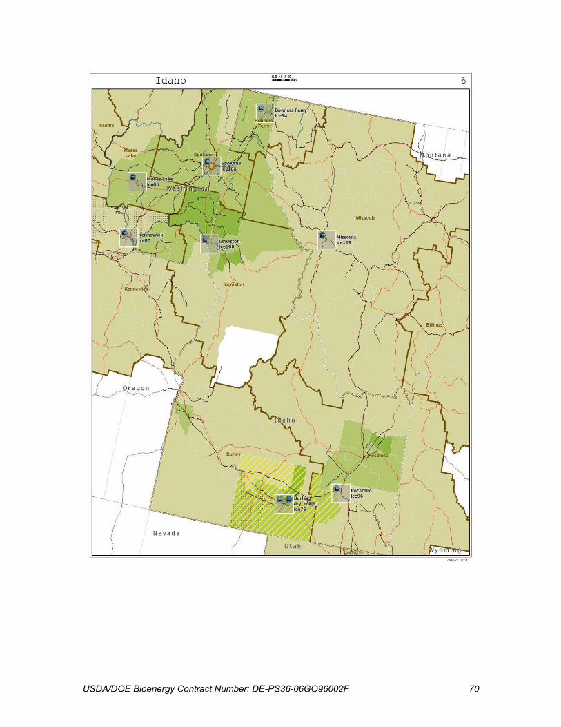
USDA/DOE Bioenergy Contract Number: DE-PS36-06GO96002F 70

USDA/DOE Bioenergy Contract Number: DE-PS36-06GO96002F 71
IDAHO SUPPLY CURVES Figure 42: Production of biofuels in Idaho and from Idaho’s resources
Figure 43: Consumption of Idaho’s biomass resources for biofuel production

USDA/DOE Bioenergy Contract Number: DE-PS36-06GO96002F 72

USDA/DOE Bioenergy Contract Number: DE-PS36-06GO96002F 73
KANSAS SUPPLY CURVES Figure 44: Production of biofuels in Kansas and from Kansas’ resources
Figure 45: Consumption of Kansas’ biomass resources for biofuel production

USDA/DOE Bioenergy Contract Number: DE-PS36-06GO96002F 74

USDA/DOE Bioenergy Contract Number: DE-PS36-06GO96002F 75
MONTANA SUPPLY CURVES Figure 46: Production of biofuels in Montana and from Montana’s resources
Figure 47: Consumption of Montana’s biomass resources for biofuel production

USDA/DOE Bioenergy Contract Number: DE-PS36-06GO96002F 76

USDA/DOE Bioenergy Contract Number: DE-PS36-06GO96002F 77
NEBRASKA SUPPLY CURVES Figure 48: Production of biofuels in Nebraska and from Nebraska’s resources
Figure 49: Consumption of Nebraska’s biomass resources for biofuel production

USDA/DOE Bioenergy Contract Number: DE-PS36-06GO96002F 78
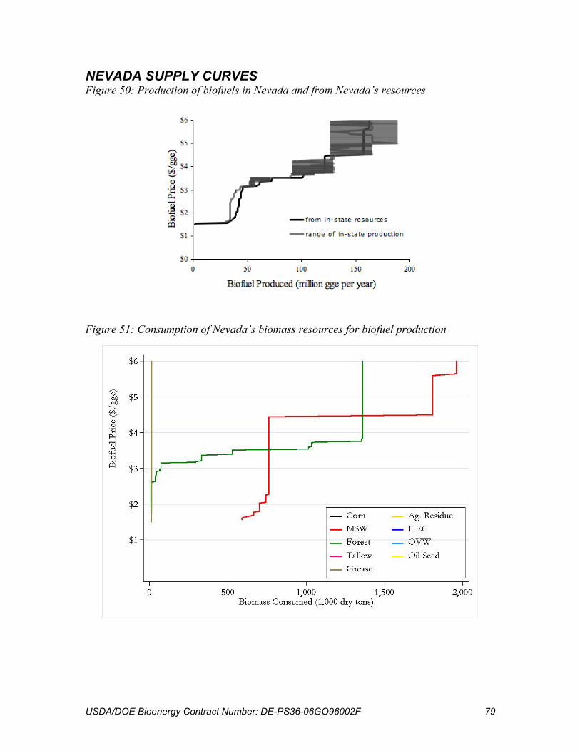
USDA/DOE Bioenergy Contract Number: DE-PS36-06GO96002F 79
NEVADA SUPPLY CURVES Figure 50: Production of biofuels in Nevada and from Nevada’s resources
Figure 51: Consumption of Nevada’s biomass resources for biofuel production

USDA/DOE Bioenergy Contract Number: DE-PS36-06GO96002F 80

USDA/DOE Bioenergy Contract Number: DE-PS36-06GO96002F 81
NEW MEXICO SUPPLY CURVES Figure 52: Production of biofuels in New Mexico and from New Mexico’s resources
Figure 53: Consumption of New Mexico’s biomass resources for biofuel production

USDA/DOE Bioenergy Contract Number: DE-PS36-06GO96002F 82

USDA/DOE Bioenergy Contract Number: DE-PS36-06GO96002F 83
NORTH DAKOTA SUPPLY CURVES Figure 54: Production of biofuels in North Dakota and from North Dakota’s resources
Figure 55: Consumption of North Dakota’s biomass resources for biofuel production

USDA/DOE Bioenergy Contract Number: DE-PS36-06GO96002F 84

USDA/DOE Bioenergy Contract Number: DE-PS36-06GO96002F 85
OKLAHOMA SUPPLY CURVES Figure 56: Production of biofuels in Oklahoma and from Oklahoma’s resources
Figure 57: Consumption of Oklahoma’s biomass resources for biofuel production

USDA/DOE Bioenergy Contract Number: DE-PS36-06GO96002F 86

USDA/DOE Bioenergy Contract Number: DE-PS36-06GO96002F 87
OREGON SUPPLY CURVES Figure 58: Production of biofuels in Oregon and from Oregon’s resources
Figure 59: Consumption of Oregon’s biomass resources for biofuel production

USDA/DOE Bioenergy Contract Number: DE-PS36-06GO96002F 88

USDA/DOE Bioenergy Contract Number: DE-PS36-06GO96002F 89
SOUTH DAKOTA SUPPLY CURVES Figure 60: Production of biofuels in South Dakota and from South Dakota’s resources
Figure 61: Consumption of South Dakota’s biomass resources for biofuel production

USDA/DOE Bioenergy Contract Number: DE-PS36-06GO96002F 90
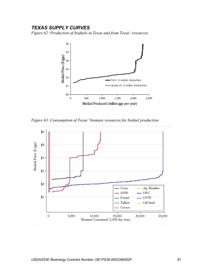
USDA/DOE Bioenergy Contract Number: DE-PS36-06GO96002F 91
TEXAS SUPPLY CURVES Figure 62: Production of biofuels in Texas and from Texas’ resources
Figure 63: Consumption of Texas’ biomass resources for biofuel production

USDA/DOE Bioenergy Contract Number: DE-PS36-06GO96002F 92

USDA/DOE Bioenergy Contract Number: DE-PS36-06GO96002F 93
UTAH SUPPLY CURVES Figure 64: Production of biofuels in Utah and from Utah’s resources
Figure 65: Consumption of Utah’s biomass resources for biofuel production

USDA/DOE Bioenergy Contract Number: DE-PS36-06GO96002F 94
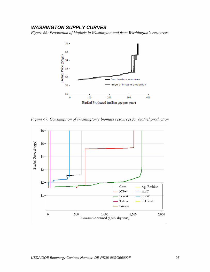
USDA/DOE Bioenergy Contract Number: DE-PS36-06GO96002F 95
WASHINGTON SUPPLY CURVES Figure 66: Production of biofuels in Washington and from Washington’s resources
Figure 67: Consumption of Washington’s biomass resources for biofuel production

USDA/DOE Bioenergy Contract Number: DE-PS36-06GO96002F 96

USDA/DOE Bioenergy Contract Number: DE-PS36-06GO96002F 97
WYOMING SUPPLY CURVES Figure 68: Production of biofuels in Wyoming and from Wyoming’s resources
Figure 69: Consumption of Wyoming’s biomass resources for biofuel production