Well Hydraulics

The time required to reach steady state depends on S(torativity) T(ransmissivity) BC(boundary conditions) and Q(pumping rate).

• cone of depression• static water level (SWL)• drawdown• residual drawdown• radius of influence• storage coefficient S• transmissivity T

Simplest SituationSteady State, Confined, inflow balances outflowOnly relationships between drawdown and distance need be considered

Only Transmissivity matters and can be determined ... Storage properties are irrelevant

Q

High T

Q

Low TSAME Q:

The shape of the drawdown cone is controlled by pumping rate Qand Transmissivity, lower T requires a higher gradient for the same Q

Darcy's Law Q=KiA is satisfied on every cylinder around the well, the gradient decreases linearly with distance from the well as the area increases linearly

STEADY STATE, CONFINED

Assuming• aquifer is homogeneous, isotropic, areally infinite• pumping well fully penetrates and receives waterfrom the entire thickness of the aquifer

• Transmissivity is constant in space and time• pumping has continued at a constant rate long enough

for steady state to prevail• Darcy's law is valid

Plot s vs log r from a number of wells as follows

s vs. log r - is a straight line, if assumptions are met, drawdown decreases logarithmically with distance form the well because gradient decreases linearly with increasing area (2πrh)

s

log r

Theim Eqtn

and rearranging to getT from field data:

T = transmissivity [L2/T]Q = discharge from pumped well [L3/T]r = radial distance from the well [L]h = head at r [L]

In an unconfined aquifer, T is not constantIf drawdown is small relative to saturated thickness, confined equilibrium formulas can be applied with only minor errorsOtherwise call on Dupuit assumptions and use:

r1

r2

observation well 1observation well 2

pumping wellQ

s1

s2

or, to determine K from field measurements of head:

Q = pumping rate [L3/T]K = permeability [L/T]hi = head @ a distance ri from well [L]

using the aquifer base as datum

The aquifer base must be the datum because the head not only represents the gradient but also reflects the aquifer thickness, hence the flow area.

More likely, vertical leakage will satisfy Q with w = recharge rate, then:

Q W = recharge rate [L/T]

We can include recharge in the expression:

and solve for K:

Q Note the confined character of the aquifer.

1. How do you know it is confined?

A Water levels in the bore that penetrates the aquifer are above the top of the aquifer.

B The aquifer is deep C Flow only occurs in the deep aquiferD There is a clay zone overlying the aquifer

A The aquifer is confined because water levels in the bore that penetrates the aquifer are above the top of the aquifer.

2. If I drilled the red well, what water level would be reflected in the well bore? A It reflects one of the blue water levels depending how long it has been since pumping beganB It will be dryC It will reflect the water level in the upper aquifer and we will not know about any of the blue water levels shown in the diagram.D It will reflect both the shallow and deep water levels

at the observation wells …..

C The red well will reflect the water level in the upper aquifer and we will not know about any of the blue water levels shown in the diagram.

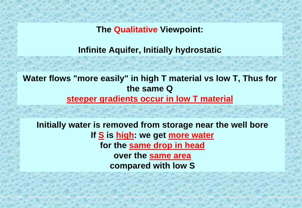
The Qualitative Viewpoint:

Infinite Aquifer, Initially hydrostatic

Water flows "more easily" in high T material vs low T, Thus for the same Q

steeper gradients occur in low T material

Initially water is removed from storage near the well boreIf S is high: we get more water

for the same drop in headover the same area

compared with low S

Sketch the relative drawdown cones for the cases below

Q Q

High S Low SSAME T Q t:

Q Q

Low THigh T SAME S Q t:

Q Q

different T yields different gradient at well boresame S yields same volume drawdown cone

but shape varies given different gradient

SAME T Q t :Q Q

High S Low S

Low THigh T

Steady state:T differences persistS differences do not

same T yields same gradient at well boredifferent S yields different volume drawdown cone

smaller S yields proportionally larger cone

SAME S Q t :

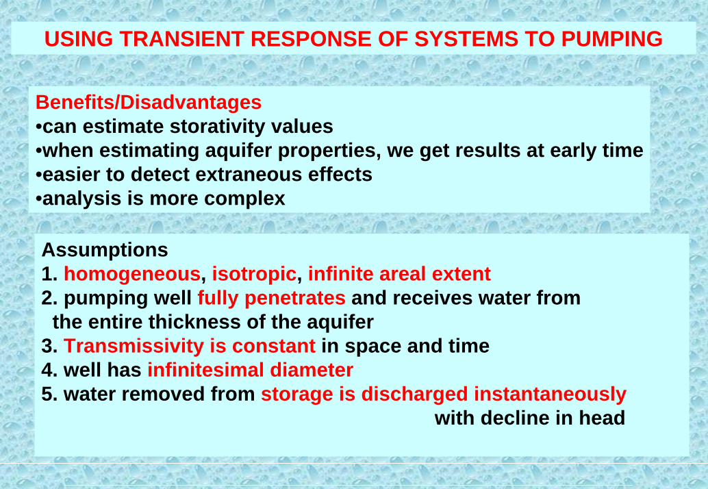
USING TRANSIENT RESPONSE OF SYSTEMS TO PUMPING

Benefits/Disadvantages•can estimate storativity values•when estimating aquifer properties, we get results at early time•easier to detect extraneous effects•analysis is more complex

Assumptions1. homogeneous, isotropic, infinite areal extent2. pumping well fully penetrates and receives water from the entire thickness of the aquifer

3. Transmissivity is constant in space and time4. well has infinitesimal diameter5. water removed from storage is discharged instantaneously

with decline in head

r1

r2

observation well 1observation well 2

pumping wellQ

s1s2

Theis Equation

s = drawdown [L]ho = initial head @ r [L]h = head at r at time t [L]t = time since pumping began [T]r = distance from pumping well [L]Q = discharge rate [L3/T]T = transmissivity [L2/T]S = Storativity [ ]

A

B

W(u

), C

urve

A

0.01

0.1

1

u, Curve A0.1 1 100.01

W(u

), C

urve

B

0.1

1

10

u, Curve B 0.10.001 0.01 1

Use of the Theis equation to determine T and S from a pumping testmatching the W(u) curve on a log-log plot s vs r2/t

sW(u)

r /t

u

2

24

41

ruTtSuW

sQT == )(

π

Cooper-Jacob simplified the Theis equation for large t and small rusing only the first 2 terms of the W(u) function

s = drawdown [L]ho = initial head @ r [L]h = head at r at time t [L]t = time since pumping began [T]r = distance from pumping well [L]Q = discharge rate [L3/T]T = transmissivity [L2/T]S = Storativity [ ]

Why are later terms notneeded?

u is small when r is smalland t is large, thus the latterterms contribute little

What is small?

Simplified expression

Since Q r T & S are constant, s vs log t should be a straight linethen:

where:

∆h = drawdown over 1 log cycle of time

to = time intercept for zero drawdown

to

∆h

Plot ∆h vs log t (for one point in time) and use:∆h drawdown over 1 log cycleto = time corresponding to ∆h=0

LEAKY AQUIFERS

Q

unpumped aquifer

pumped aquifer aquitard

b2 K2 Ss2

b1 K1 Ss1

b’ K’ Ss’ previously K’ was zero(i.e. no leakage)

subscript 1 = pumped zonesubscript 2 = unpumped aquiferprime = aquitard

Q = pumping rateb = thicknessK = hydraulic conductivitySs = specific storage

assume:no head change in shallow aquiferhorizontal flow in aquifersvertical flow in aquitardsaquifer extends far enough to

intercept enough leakage to satisfy QTheis assumptions

(other than infinite aquifer) apply

What conditions justify assuming no head change in the shallow aquifer?A sufficiently permeable shallow aquifer such that flow to the “disk” abovethe drawdown cone is low enough to require nearly zero gradient.Solution is similar to Theis Solution but well function is more complex

Q

What will happen that did not occur in the completely confined aquifer?

water level in shallow aquifer

Vertical leakage, first from storage in the aquitard, thenfrom the shallow aquifer.

What do we expect regardingthe magnitude of leakage?Greatest leakage where head difference is largest,decreasing away from the well.

What will be the maximum extent of drawdown?Drawdown will be limited to the radius at which the entire Q leaks from the upper aquifer to the lower.

What controls the rate of drawdown cone development?

Transients will occur as the head decrease moves up through the aquitard. S and Kvof the aquitard will control the rate of progress.

will the red observation well look more like? …..

log

s dr

awdo

wn

log time

C recharge boundary

B infinite aquifer

A no-flow boundary

D none of the above

Hantush & Jacob 1955assumed no storage in the aquitardand expressed this solutionin terms of a dimensionless parameter

Curve matchW(u, r/B) r/B 1/u matched with s t

Solve for K1 from

Solve for K’ from

Solve for S1 from

Q=0.004 m3/sec b1=30.5m r=55m b’=3.05m

W(u,r/b)=0.6 (r/B=1.0)s=0.08m

1/u=0.8150 sec

Q=0.004 m3/sec b1=30.5m r=55m b’=3.05m

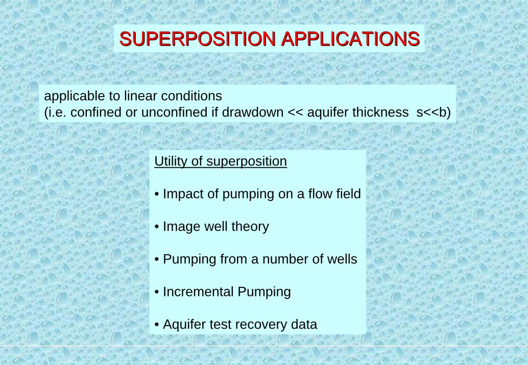
SUPERPOSITION APPLICATIONSSUPERPOSITION APPLICATIONS

applicable to linear conditions (i.e. confined or unconfined if drawdown << aquifer thickness s<<b)

Utility of superposition

• Impact of pumping on a flow field

• Image well theory

• Pumping from a number of wells

• Incremental Pumping

• Aquifer test recovery data

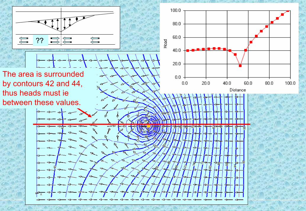
IMPACT OF PUMPING ON A FLOW FIELDDrawdown from pumping is superimposed on the initial flow field

( i.e. subtract drawdown from undisturbed piezometric head)

ground surface

confined aquifer

original piezometric surface

??

What happens here?How can water flow both ways?Is water "created" at this location?

piezometric surfaceafter pumping

??

From the contours of head, how do you know the head is higher than 42 in this area?

The area is surrounded by contours 42 and 44, thus heads must iebetween these values.

Q Impermeable or No-flow Boundary

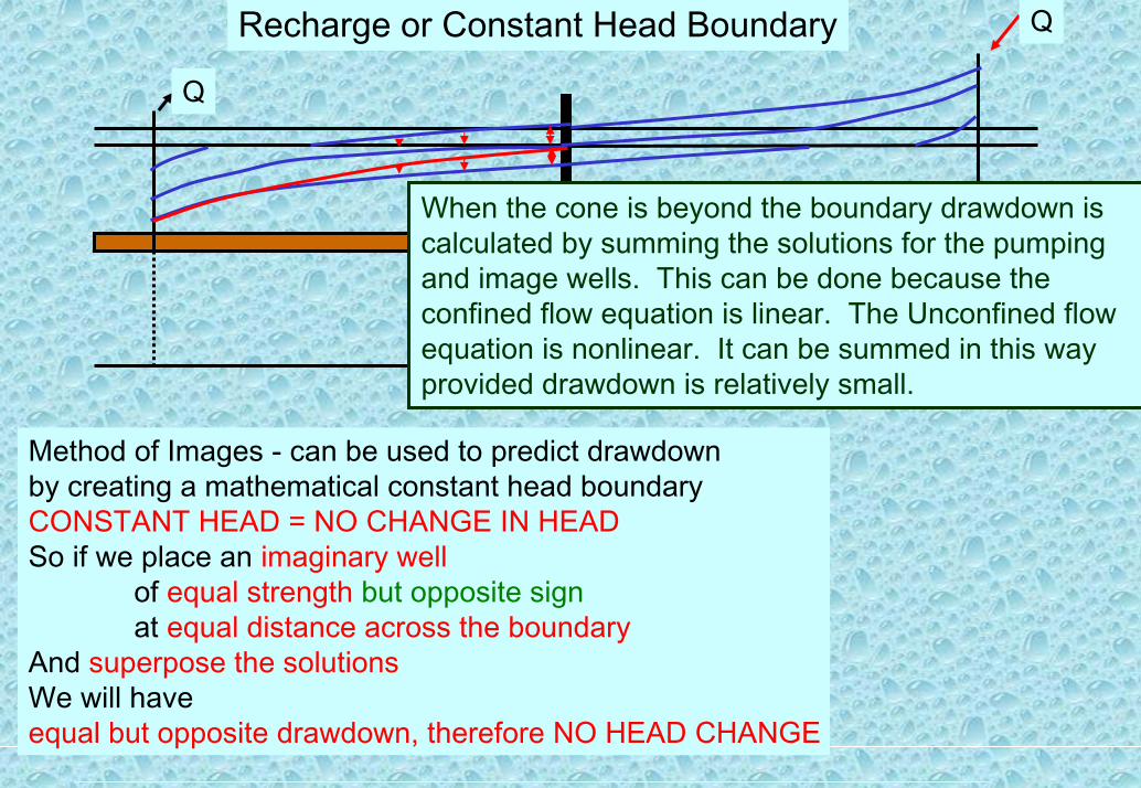
Q Recharge or Constant Head Boundary

IMAGE WELL THEORY Impact of Boundaries on drawdown as a function of time

No aquifer is infinite. How will boundaries affect response?

For the following situation with pumping well Q make your qualitative estimates of the relative drawdown. Sketch the cone of depression due to

pumping of well Q assuming A-A’ is a no flow boundary

Sketch the cone of depression due to pumping of well Q assuming the aquifer is infinite

Sketch the cone of depression due to pumping of well Q assuming A-A’ is a constant head boundary

Q

at the red observation well …..

log

s dr

awdo

wn

log time

recharge boundary

infinite aquifer

no-flow boundary

Q Impermeable or No-flow Boundary

When the drawdown cone reaches the boundary water cannot be drawn from storage in the infinite aquifer, so drawdown occurs more rapidly within the finite aquifer

Impermeable or No-flow BoundaryQ Q

Before the drawdown cone reaches the boundary the drawdown curve is as predicted by the Theis equationWhen the cone reaches the boundary this is the last moment that the drawdown curve will be as predicted by the Theis equation. Note drawdown from both wells is equal thus there is no difference in head across the boundary, so the gradient is zero and there is no flow.

When the cone is beyond the boundary drawdown is calculated by summing the solutions for the pumping and image wells. This can be done because the confined flow equation is linear. The Unconfined flow equation is nonlinear. It can be summed in this way provided drawdown is relatively small.

Method of Images - can be used to predict drawdown by creating a mathematical no-flow boundaryNO-FLOW = NO GRADIENTSo if we place an imaginary well

of equal strength at equal distance across the boundary

and superpose the solutions, we will have equal drawdown, therefore equal head at the boundary, hence NO GRADIENT

Plan View

image well

r2 r1

pumping well

observation well

This side of boundary is all a mathematical construct

x x

calculate s @ r1

calculate s @ r2

no-flow boundary (eg very low K material)

sum s @ r1 and s @ r2 drawdown is greater than without the boundary

Q

Recharge or Constant Head Boundary Q

Before the drawdown cone reaches the boundary the drawdown curve is as predicted by the Theis equationWhen the cone reaches the boundary this is the last moment that the drawdown curve will be as predicted by the Theis equation. Note drawdown equals drawupthus the head has not changed at the boundary.

When the cone is beyond the boundary drawdown is calculated by summing the solutions for the pumping and image wells. This can be done because the confined flow equation is linear. The Unconfined flow equation is nonlinear. It can be summed in this way provided drawdown is relatively small.

Method of Images - can be used to predict drawdown by creating a mathematical constant head boundaryCONSTANT HEAD = NO CHANGE IN HEADSo if we place an imaginary well

of equal strength but opposite signat equal distance across the boundary

And superpose the solutionsWe will have equal but opposite drawdown, therefore NO HEAD CHANGE

Plan View

image wellpumping well

observation well

r2 r1

This side of boundary is all a mathematical construct

x x

calculate s @ r1

calculate s @ r2 S is negative due to Q of injection being negative

recharge boundary (eg fully penetrating stream)

sum s @ r1 and s @ r2 drawdown is less than without the boundary

PUMPING FROM A NUMBER OF WELLS

where:

location of interest

Plan View

r1

pumping wellcalculate s @ r1

r2

injection wellcalculate s @ r2

r3 pumping wellcalculate s @ r3

sum s1 from Q1@ r1 s2 from Q2@ r2 (note Q2 is negative) s3 from Q3@ r3 ….. etc etc ….. yields total s at observation well

INCREMENTAL PUMPING

startt=0

Q1 = initial rate u1 for t since pumping started, t1

∆Q2 = Q2 - Q1 u2 for t since incremented rate, t2

∆Q3 = Q3 - Q2 u3 for t since second increment, t3

t1

pumping starts at Q1

pumping changes to Q2,calculate s for Q2 -Q1

t2The sum of all threecalculations yieldss at t1 for the varyingflow rate

pumping changes to Q3 ,calculate s for Q3 –Q2

t3

AQUIFER TEST RECOVERY DATAadding drawdown from injection of –Q at the time when the pump is shut off

startt=0 t

pumping starts at Q1

t’

pumping stops at t=t’equivalent to incremental pumping of - Q1

t’=0t is always this much larger than t’

t

s = 0

t=0

t’t’=0

For small u (small r, long t) the Cooper-Jacob relation can be used:

Plot of s’ vs log(t/t’) is a straight line

∆s over one log cycle t/t'