Embed Size (px)
Citation preview

71
CATHERINE HAUSMANUniversity of Michigan
RYAN KELLOGGUniversity of Michigan
Welfare and Distributional Implications of Shale Gas
ABSTRACT Technological innovations in horizontal drilling and hydrau-lic fracturing have enabled tremendous amounts of natural gas to be extracted profitably from underground shale formations that were long thought to be uneconomical. In this paper, we provide the first estimates of broad-scale wel-fare and distributional implications of this supply boom. We provide new esti-mates of supply and demand elasticities, which we use to estimate the drop in natural gas prices that is attributable to the supply expansion. We find large, positive welfare impacts for four broad sectors of gas consumption (residential, commercial, industrial, and electric power) and a negative impact for producers, with variation across regions. We then examine the evidence for a gas-led “manufacturing renaissance” and for pass-through to prices of products such as retail natural gas, retail electricity, and commodity chemicals. We conclude with a discussion of environmental externalities from unconventional natural gas, including limitations of the current regulatory environment. Overall, we find that between 2007 and 2013 the shale gas revolution led to an increase in welfare for natural gas consumers and producers of $48 billion per year, but more data are needed on the extent and valuation of the environmental impacts of shale gas production.
Following a decade of essentially no growth, natural gas production in the United States grew by more than 25 percent from 2007 to 2013.
This supply boom, amounting to an increase of 5.5 trillion cubic feet a year, was driven by technological innovations in extraction. In particular, advances in horizontal drilling and hydraulic fracturing, or “fracking,” have enabled natural gas to be extracted profitably from underground shale formations that were long thought to be non-economic. Figure 1 shows

72 Brookings Papers on Economic Activity, Spring 2015
this increase in total natural gas production as well as the change in pro-duction from unconventional shale gas reservoirs. The increase in shale extraction began in the late 2000s, accelerated in 2010, and amounted to more than one trillion cubic feet a month by late 2013. As a result of this sustained growth in extraction, natural gas prices have fallen substantially in the United States. Figure 1 plots the real1 U.S. price of natural gas since 1997.2 While prices averaged $6.81 per thousand cubic feet (mcf) (in 2013 dollars) from 2000 to 2010, prices since 2011 have averaged $3.65 per mcf.
In this paper, we estimate the broad implications of this boom in unconventional natural gas for U.S. welfare. We examine the effects on natural gas purchasers and producers, paying particular attention to how benefits and costs are allocated across sectors and across space. We also
1. Prices throughout the paper are deflated to 2013 dollars using the CPI (all urban less energy).
2. We focus on the Henry Hub price in Louisiana, the most liquidly traded natural gas hub in the country. Prices are quoted in $/mmBtu (dollars per million British thermal units), and we convert this to $/mcf (dollars per thousand cubic feet). The heat content of natural gas varies, but the average conversion typically used is 1.025 mmBtu per mcf.
Figure 1. U.S. Natural Gas Production and Price, 1997–2015
Bcf per dayReal dollars per mcf
20
40
60
80
5
10
15
1997m1 2000m1 2003m1 2006m1 2009m1 2012m1
Henry Hub price
Natural gas withdrawalsa
Natural gas withdrawals from shalea
Source: EIA.a. Gross withdrawals include not only marketed production, but also natural gas used to repressure wells,
vented and flared gas, and nonhydrocarbon gases removed.

CATHERINE HAUSMAN and RYAN KELLOGG 73
discuss the potential environmental impacts associated with fracking and how regulations might mitigate these externalities.
We begin in section I by providing background on natural gas markets, including the related literature on fracking. We then provide new estimates of supply and demand elasticities. In section II, we use our estimated sup-ply and demand functions to calculate the portion of the drop in natural gas prices that is attributable to the supply expansion, as opposed to contempo-raneous changes in the U.S. economy such as the recession and recovery. For the period 2007–13, we estimate that the boom in U.S. natural gas production reduced gas prices by $3.45 per mcf.
We evaluate the impact of the supply shift and corresponding price change for consumers and producers in section III. There we show that consumer surplus increased by about $74 billion a year from 2007 to 2013 because of the price fall. In contrast, producer surplus fell: wells, once they are drilled and producing, have very low marginal operating costs and are rarely idled. Thus, from 2007 to 2013, revenue accruing to pro-ducers of existing wells declined by $30 billion a year owing to the price decrease. This loss was only partially offset by the gains associated with new wells, which totaled $4 billion a year over this period. Accordingly, we estimate that annual total welfare increased by $48 billion from 2007 to 2013, ignoring external costs from environmental damages (to which we return later in the paper). Under plausible alternative assumptions, this esti-mate varies by up to about 20 percent. This change in surplus (consumer and producer) is large relative to the size of the natural gas sector; retail spending on natural gas was around $160 billion in 2013. On the scale of the economy as a whole, it is noticeable but not large—the change amounts to about ¹⁄³ of 1 percent of GDP, or around $150 per capita.
We also consider the distributional effects of the supply boom across sectors of the economy and across regions. Purchasers of natural gas can be broadly separated into the residential, commercial, industrial, and electric power sectors. We calculate the breakdown in consumer surplus changes across these four sectors and find that the largest gains were in the electric power and industrial sectors. We then estimate the distribution of consumer gains across states. There we find the largest gains concentrated in the South Central and Midwestern states, where industrial and electric power demand for gas is large. Regional variation in the impact of shale gas on the producer surplus is substantial; shale-heavy states like Pennsylvania experienced net gains, whereas states with mostly conventional gas supplies experienced net loss. Finally, we examine the pass-through of changes in the natural gas wholesale price to end-users. We find that the pass-through to

74 Brookings Papers on Economic Activity, Spring 2015
retail prices is essentially 100 percent, implying that the consumer surplus gains we estimate have accrued to end-users of gas rather than to distribu-tors or retailers.
In section IV, we study how exports of liquefied natural gas (LNG) would affect gas purchasers and producers. Natural gas is costly to ship overseas: it must be liquefied (by chilling it to an extremely low temperature and placing it under high pressure), then shipped on specialized LNG tankers, and then re-gasified at the final destination. Moreover, the construction of LNG facilities and the export of LNG require approval from the Federal Energy Regulatory Commission (FERC) and the federal Department of Energy (DOE), respectively.
A considerable wedge has developed since 2010 between the relatively low natural gas prices in the United States and prices in Europe and Japan, as shown in the left panel of figure 2.3 This price differential has led firms
3. The price differential between the United States and Asia has shrunk somewhat in early 2015, since Asian LNG prices are tied at least in part to crude oil prices, which have fallen substantially.
5
10
15
Real dollars per mcf
1998m1 2006m1 2014m1
Japan LNG
UK NBP natural gasb
Henry Hub natural gasa
50
100
Real dollars per barrel
1998m1 2006m1 2014m1
Brent crude oil
West Texas International crude oil
Source: EIA for Henry Hub, West Texas International, and Brent spot prices; Bloomberg for the UK National Balancing Point (NBP) spot price; World Bank for the Japan LNG price.
a. The Henry Hub price is a monthly average of the daily NYMEX spot price. b. The UK price is a monthly average of the daily NBP price; it has been converted here from GB pence per
therm to US$ per mcf.
Figure 2. U.S. and International Natural Gas and Crude Oil Prices, 1998–2014

CATHERINE HAUSMAN and RYAN KELLOGG 75
to apply for LNG export permits. We use our modeling framework to simu-late how the U.S. gas market would be affected by (i) LNG exports equal to the capacity of all FERC-approved projects (9.2 billion cubic feet [bcf] per day), and (ii) LNG exports equal to the capacity of all projects approved by and proposed to FERC (24.6 bcf per day). In both cases the U.S. natural gas price would rise, leading to an increase in U.S. producer surplus, a decrease in the U.S. consumer surplus, and a net gain overall. However, the net gain is limited (and nearly zero in the first case) because a share of the increase in overall producer surplus accrues to Canadian exporters of natural gas to the United States.
In section V we consider the impacts of shale gas on manufacturing at a more disaggregated level, motivated by the considerable interest in whether shale gas will lead to a U.S. “manufacturing renaissance.” We identify industries that are especially natural-gas-intensive in production and therefore have the potential to benefit the most from the shale boom. A handful of manufacturing sectors stand out as important, especially fertilizer production. We find that these sectors have grown more rapidly than other sectors over the course of the shale boom, though drawing a conclusive causal link is difficult. We document that the fertilizer indus-try has substantially expanded, likely owing to the fact that U.S. fertilizer prices are integrated with global markets and have therefore not greatly decreased. We find a similar pricing pattern for high-density polyethylene, a common plastic that uses natural gas as an input. Thus, at least for these gas-intensive chemical products, reductions in gas prices have not passed through to product prices.
Finally, there are important unpriced environmental impacts associated with shale gas production. Scientists have identified a long list of poten-tial impacts, such as groundwater contamination and methane leaks. In section VI, we present the state of the literature on these effects. We note several challenges for monetization: there is a lack of comprehensive data on physical damages, and the spatial heterogeneity of impacts prohibits a comprehensive bottom-up aggregation. Additionally, both local and global impacts depend on the extent to which coal has been displaced, something about which there is still uncertainty. Because of these uncertainties, we estimate that valuation of greenhouse gas impacts in 2013, for instance, ranges from a net cost of $3.0 billion to a net cost of $28 billion. We also discuss the challenges associated with collecting comprehensive data on environmental impacts, as well as the implications of these data limitations for regulation of the industry.

76 Brookings Papers on Economic Activity, Spring 2015
While this paper focuses on natural gas, it is important to note that a shale oil fracking boom has been taking place alongside the boom in natu-ral gas (see Kilian 2014a). Oil production in the United States increased by almost 50 percent from 2007 to 2013, enabled by the same technological improvements driving the natural gas boom. Moreover, oil prices fell dra-matically in 2014: from around $100 a barrel in Q1 and Q2 to around $50 a barrel by the start of 2015. We focus here on natural gas in part because it has historically received less attention in the literature.4 Future work on recent changes to oil markets, driven by unconventional sources, would certainly be valuable. Natural gas and oil markets have some similarities, since they are both exhaustible resources, are substitute inputs for one another in some industries, and are extracted using similar technologies, but they also have some key differences. In particular, crude oil is easily shipped internationally, so the world oil market is largely integrated.5 In contrast, natural gas is easy to transport by pipeline but is otherwise costly to ship. The shale oil boom has resulted in some transportation-related and grade-related bottlenecks and therefore wedges between the U.S. and world oil prices (Borenstein and Kellogg 2014, Brown and others 2014, Kilian 2014a). The right panel of figure 2 shows how the Brent (North Sea) price has increased relative to the U.S. West Texas Intermediate price since 2010. However, this oil price differential is small compared to the recent wedge in natural gas prices between North America and markets in Europe and Asia.
Overall, our study finds that a broad set of sectors has benefited from new sources of unconventional natural gas. Households, for instance, have seen much lower utility bills for both natural gas and electricity. Industrial users have also benefited, including rents for some natural-gas-intensive industries that have not had to pass on the lower gas prices to their customers. Natural gas producers, on the other hand, have seen substantial revenue declines that have been only partially offset by the shale-driven expansion of drilling and production. The full scope of external environmental costs is still unknown, and better data are needed in this area.
4. Excellent recent examples of work studying the link between oil and the macro-economy include Hamilton (2009); Kilian (2009); Hamilton (2011); Kilian (2014b), and Kilian and Murphy (2014).
5. Though the United States remains a net importer of crude oil, the U.S. crude oil export ban binds due to crude quality differences. See Kilian (2014a) for a discussion.

CATHERINE HAUSMAN and RYAN KELLOGG 77
I. Fundamentals of the U.S. Natural Gas Market
Natural gas marketed production in the United States was approximately 50 bcf per day from 1990 through 2007, primarily from gas extracted in Texas, Louisiana, and Oklahoma.6 From 2007 to 2013, U.S. production increased by 25 percent. This sharp acceleration of production was spurred by technological advances in horizontal drilling and hydraulic fracturing (or fracking). While horizontal drilling and fracking have been in use for half a century, they only recently became cost-effective for large-scale gas extraction. Reservoirs that have seen substantial activity include the Barnett shale in Texas and the Marcellus shale in Pennsylvania.
Our paper relates to a nascent economics literature on the shale boom, including work that, like ours, devotes its attention to broad economic impacts. Timothy Fitzgerald (2013) offers a useful summary of stylized facts about the fracking boom, including summaries of the technological changes and their impact on the cost of extraction. Charles Mason, Lucija Muehlenbachs, and Sheila Olmstead (2014) provide a summary of the lit-erature on shale gas in economics as well as a broad first pass at calculating the scope of economic costs and benefits. Alan Krupnick and others (2014) summarize policy questions that remain unanswered relating to economic impacts, environmental impacts, and preferred regulatory approaches. Other related work has used calibrated models of the energy sector to fore-cast future impacts of shale gas production (Brown and Krupnick 2010, Krupnick, Wang, and Wang 2013), and a growing literature examines how falling natural gas prices affect electricity markets (Brehm 2015, Cullen and Mansur 2014, Holladay and LaRiviere 2014, Knittel, Metaxoglou, and Trindade 2014, Linn, Muehlenbachs, and Wang 2014). The Congressional Budget Office recently issued a report aimed at projecting future economic and budgetary impacts of shale oil and gas (CBO 2014). Local employ-ment effects near extraction sites have been analyzed by Mark Agerton and others (2015), Hunt Allcott and Daniel Keniston (2014), Thomas DeLeire, Paul Eliason, and Christopher Timmins (2014), Peter Maniloff and Ralph Mastromonaco (2015), and Dusan Paredes, Timothy Komarek, and Scott Loveridge (2015). In section VI, we summarize the large literature, span-ning many disciplines, on the environmental impacts of fracking.
6. While figure 1 plots gross withdrawals of natural gas, we focus for the remainder of the paper on marketed production. Marketed production averages 80 to 85 percent of gross withdrawals and does not include, for instance, reinjections. Figure 1 plots gross withdrawals because marketed production specific to shale is not available.

78 Brookings Papers on Economic Activity, Spring 2015
I.A. Demand and Supply Estimation: Empirical Strategy
Our paper is the first to provide a comprehensive analysis of the wel-fare impacts of the shale gas boom for purchasers and producers, including the distribution of these impacts across consumption sectors and across space. An important first step in our analysis is the estimation of supply and demand functions for natural gas, and in particular the elasticities of supply and demand. These elasticities are essential inputs into the calculation of the U.S. natural gas price that would have held in 2013 had the shale gas revolution not expanded supply. Specifically, we will calculate the counter-factual equilibrium price of gas at the intersection of the 2007 supply curve with the 2013 demand curve; we need the elasticities of both supply and demand to identify this intersection relative to the realized 2007 and 2013 equilibria. With the counterfactual 2013 natural gas price in hand, we can then use the estimated supply and demand curves to estimate changes in consumer and producer surplus associated with fracking.
While some elasticity estimates exist in the literature (Davis and Muehlegger 2010, Arora 2014), they are not available for all sectors. We begin by estimating the short-run and long-run elasticities of natural gas demand. Consider a dynamic equation for natural gas consumption in state i in month t, Cit, in which adjustment costs lead to an AR(1) process:
(1) log log log ., 1C P C W tit C it C i t C C C C Cit it it= α + γ + β + μ + δ + ε−
In equation 1, gas consumption is affected by the current-period retail gas price Pit, observed weather WCit
, state-specific seasonality μCit, a secular
trend, and a disturbance term εCit, which includes unobservable shocks to
energy-consuming economic activity. We model demand as a dynamic pro-cess because we anticipate that purchasers’ adjustments to price shocks will be gradual. For instance, agents might react to high natural gas prices by making investments in energy efficiency; these investments usually require more than a single month to complete. We focus for simplicity on an AR(1) specification, but results are robust (as shown in the online appendix)7 to inclusion of Ci,t−2 as an explanatory variable. Nonetheless, due to the lim-ited duration of our sample, our estimate of equation 1 may understate the
7. The online appendix to this and other papers in this volume may be found at the Brookings Papers webpage, www.brookings.edu/bpea, under “Past Editions.”

CATHERINE HAUSMAN and RYAN KELLOGG 79
true long-run demand elasticity, which could include out-of-sample capital replacement and innovation, such as widespread deployment of natural- gas-powered vehicles. Below, we consider bounding exercises on our wel-fare estimates that allow for a substantially larger elasticity than what we estimate from equation 1.
Because natural gas consumption and prices are simultaneously deter-mined by the interaction of demand and supply, OLS estimation of equa-tion 1 will be biased: the estimated magnitude of the demand elasticity αC will be too low. To address this problem, we leverage the intuition from two previous papers that confront a similar issue. First, Lucas Davis and Erich Muehlegger (2010) estimate a natural gas demand elasticity from state-level data using weather shocks in other states as an instrumental variable (IV). The intuition is that because much of natural gas is used for space heating, cold weather drives up demand and therefore price. To show the importance of space heating, figure 3 plots demand by month for each sector. The space heating impact leads to large seasonality for residential and commercial users; industrial demand also increases in the
Figure 3. U.S. Natural Gas Consumption by Sector of End Use, 2010–14a
0
10
20
30
Bcf per day
2010m1 2011m1 2012m1 2013m1
Commercial
Electric power
Net exports
Source: EIA.a. Natural gas used in vehicles, in drilling operations, and as fuel in natural gas processing plants is not shown,
but all these amounts are small.
Residential
Industrial

80 Brookings Papers on Economic Activity, Spring 2015
winter but is much less seasonal. Natural gas use in the electric power sector, in contrast, follows demand for electricity, and accordingly spikes in the summer.
The intuition for the validity of the Davis and Muehlegger (2010) instru-ment is that weather shocks in states other than i will be correlated with the natural gas price in state i because U.S. gas markets are well integrated. At the same time, weather shocks in other states should not directly affect natural gas consumption in state i, after controlling for weather shocks in state i. To ensure that the instrument captures weather shocks and not sea-sonality, Davis and Muehlegger (2010) control for state by month effects.
We do not rely solely on this approach, however, because we estimate a weak first stage. That is, after controlling for a state’s own weather, there is little variation left in other states’ weather.8 We therefore also take advan-tage of the theory of competitive storage, an approach that has been used in prior work to understand agricultural markets (Roberts and Schlenker 2013). The intuition is that the price at which suppliers are willing to deliver gas is a function of the volume of gas in storage. Storage volumes at time t will be a function of shocks in previous periods; thus, lagged values of WCit
are valid instruments for Pit in equation (1).9 For instance, cold weather in month t − k will drain gas storage reserves, increasing the gas price in peri-ods t − k through t (and beyond).10
We incorporate the intuition from both Davis and Muehlegger (2010) and Michael Roberts and Wolfram Schlenker (2013) by using lags of weather in states other than i as our instrumental variable. In practice, we operationalize WCit
using heating degree days (HDDs), a measure of cold weather that is commonly used to approximate space heating requirements.11 For each state-month observation it, we then construct the IV as follows: we calculate population-weighted average HDDs for each month for all states in other regions (defined as census divisions)
8. Davis and Muehlegger (2010) also include the Brent crude oil price as an addi-tional IV. This instrument requires that demand shocks be uncorrelated across oil and natural gas markets.
9. Lagged prices and consumption could also be valid instruments; however, the valid-ity of these IVs requires that εCit
not be serially correlated.10. We verified this intuition empirically by regressing inventories (in levels or changes)
on cold weather, controlling for month effects. We estimate negative and statistically signifi-cant effects of cold weather, lasting for around 6 to 8 months.
11. On any given day, the number of heating degrees is given by min (0, 65 − T), where T is the day’s temperature in degrees Fahrenheit. We then average across days in the month. Cooling degree days (CDDs) are analogous to HDDs and are given by min (0, T − 65).

CATHERINE HAUSMAN and RYAN KELLOGG 81
and then sum these averages over lags 2 through 12. We sum across lags 2 through 12 for two reasons. First, the effect of weather on storage is cumu-lative; prices will likely increase more when unexpected draw-downs have occurred in multiple prior months. Second, we want the second-stage to be identified off of price variation in all months, not only months with cold weather. Otherwise, our estimated elasticity would only be appropriate for winter months.
We control for current weather (as measured by heating and cooling degree days), one-month lagged weather, state by month effects, and a linear time trend. Since we identify off of variation in weather shocks, the linear time trend is not necessary for unbiased estimates, but it does aid with precision. Conditional on these controls, we thus make fairly weak assumptions to obtain identification: the exclusion restriction is satisfied as long as two-month through twelve-month lagged weather shocks in regions other than i are conditionally uncorrelated with demand shocks in region i. For this to be satisfied, we simply need any impact of past weather on current consumption to be picked up in the AR(1) term. Standard errors are two-way clustered by sample month and state.
Our strategy for estimating the natural gas supply elasticity is conceptu-ally very similar to that for demand. We again use the behavior of storage to motivate our instrument—in fact, the same instrument can be used for the supply equation. Conceptually, anything that drives down storage vol-umes in previous months will increase price in the current month, affecting both current supply and demand. Since storage volumes can fluctuate, sup-ply need not equal demand in any given month; thus, the same instrument can be used for both equations. In practice, there are a few operational differences in the way we implement this idea. First, we use national rather than state-level quantities and prices because of data limitations. Second, we use the wholesale Henry Hub natural gas price rather than retail natural gas prices; results are similar if we use the average wellhead price instead of Henry Hub. Third, we found that power in the first stage was aided by using one-month lagged HDDs and CDDs (cooling degree days) rather than cumulative HDDs.
Rather than use natural gas production in month t as the dependent vari-able, we use the number of wells drilled in month t.12 We do so because oil and gas producers respond to price shocks not by changing the production rate of existing wells but by changing the rate at which they drill new wells
12. Online appendix figure A1 shows a time series of natural gas drilling.

82 Brookings Papers on Economic Activity, Spring 2015
(Anderson, Kellogg, and Salant 2014).13 Thus, the supply equation we esti-mate is given by:
(2) log log log .1S P S W tt S t S t S S S S St t t= α + γ + β + μ + δ + ε−
where St is the numbers of wells drilled.14 We again control for month-of-year effects to isolate weather shocks from seasonality, and we include a linear time trend for precision. We also control for current weather because it may be correlated with our instrument (past weather) and it may affect current drilling operations. As in the demand specifications, we show (in the online appendix) that results are robust to inclusion of St−2 on the right-hand side. Finally, standard errors are Newey-West with 17 lags.
Our data source for consumption and retail prices is the Energy Infor-mation Administration (EIA). The data are at the state-by-month level for 2001 to present, and they are broken down into residential, commercial, electricity sector, and other industrial usage.15 Because the electricity sector price has many missing values, our preferred electric power specification uses the citygate price, also available from the EIA.16 Our data source for monthly natural gas production and the number of wells drilled is also the EIA. The drilling data, which we use for the elasticity estimation, are
13. Moreover, in the drilling and production model of Anderson, Kellogg, and Salant (2014), the long-run drilling elasticity equals the long-run production elasticity, assum-ing that resource scarcity rents are small, because steady-state production is proportional to steady-state drilling. A few caveats are necessary here. First, we are assuming that productivity from wells drilled when prices are high is the same as productivity from wells drilled when prices are low. Second, the time horizon at which the elasticities are approximately equal may be longer than the period we consider. Finally, some natural gas is extracted from oil wells, which likely have a lower elasticity with respect to natural gas prices. Below we consider bounding cases on the price and welfare impacts using both a higher and lower elasticity.
14. More specifically, the data track wells drilled and “completed,” that is, ready for production.
15. Total consumption is available farther back, but electricity and industrial consump-tion data only begin in 2001. For consistency across sectors, we use 2001 through 2013. The demand regressions do not include Alaska, the District of Columbia, or Hawaii. Addition-ally, some of the electricity sector usage data are “withheld to avoid disclosure of individual company data.” These are from states with low levels of usage. Also, some states report zero electricity sector usage for some months; we replace with ln(0.1), but results are similar if we drop these observations.
16. The two prices are highly correlated, and results are similar if we use the electric power price instead. The “citygate” is the point where natural gas is typically delivered from interstate pipelines to the local distribution utility.

CATHERINE HAUSMAN and RYAN KELLOGG 83
monthly, but unfortunately they are not available at the state level and have not yet been released for recent years (2011–14). For production, we focus on marketed production rather than gross withdrawals, as the latter include gas reinjected into wells. Marketed production is available for a few states with substantial production (such as Texas, Louisiana, and Oklahoma), while other states are aggregated together. In the supply estimation, we use average monthly spot prices from Bloomberg. We focus on the price at Henry Hub, Louisiana, which is the delivery point for liquidly traded natu-ral gas futures contracts. Henry Hub is also typically well integrated with other U.S. natural gas markets. Finally, we use monthly state-level weather data (heating and cooling degree days) from the National Climatic Data Center at the National Oceanic and Atmospheric Administration.
I.B. Elasticity Estimation Results
Our primary natural gas demand and supply estimates are presented in table 1 below. The demand elasticity varies by sector, although the dif-ferences are not statistically significant. The industrial and electric power sectors are most elastic, with short-run price elasticities of −0.16 and −0.15, respectively. The long-run elasticities, equal to αC(1 − γC), are −0.57 and −0.47, with standard errors of 0.17 and 0.43. The residential and commer-cial sectors have short-run elasticities of −0.11 and −0.09, respectively, with long-run elasticities of −0.20 and −0.23 (the standard errors on the long-run estimates are 0.19 and 0.18).17 The estimated short-run supply elasticity, αS, is 0.09. The long-run elasticity is 0.81, with a standard error of 0.16.
Unfortunately, the estimates are imprecise. However, as we show and discuss in section II, the overall welfare gain we calculate is qualitatively quite robust to reasonable alternate elasticities. Conceptually, the large standard errors are not surprising. Our identifying variation comes largely from movements in prices in response to national weather shocks, so the specifications are akin to time-series regressions using 11 years of monthly data for demand and 9 years of monthly data for supply.18
In the online appendix (tables A4, A5, A6, and A7) we consider a num-ber of additional robustness checks, including alternative instruments (such
17. Summing across the four sectors, the demand equation no longer has constant elas-ticity. For the range of quantities observed in our data, the long-run elasticity of total demand is about −0.4.
18. Conventional rather than clustered standard errors, as a result, would have been only about half as large for the demand equations. For the supply equation, conventional standard errors are slightly larger than the Newey-West results we report.

84 Brookings Papers on Economic Activity, Spring 2015
as shorter and longer weather lags and regional weather) and alternative controls. It is reassuring that the results, in particular the long-run elastici-ties, are generally very similar using these alternative specifications. Our short-run elasticities are smaller than those from Davis and Muehlegger (2010), who report an average short-run elasticity of −0.28 for residential, −0.21 for commercial, and −0.71 for industrial users. Vipin Arora (2014) estimates a long-run residential demand elasticity of −0.24, and a long-run supply elasticity ranging from 0.10 to 0.42.
Online appendix tables A2 and A3 provide first-stage estimates for the demand and supply specifications in table 1. For all four demand sectors, the instrument—cumulative lagged HDDs in other states—has a positive and statistically significant effect on the natural gas price, as expected. For supply, the instruments—lagged national HDDs and CDDs—also have a positive effect on the natural gas price.
Table 1. Demand and Supply Elasticity Estimatesa
Demand b
Supply c
DrillingResidential Commercial IndustrialElectric power
log(Price) −0.11 −0.09 −0.16 −0.15 0.09(0.11) (0.08) (0.07) (0.14) (0.05)
yt−1 0.43 0.59 0.72 0.68 0.89(0.05) (0.04) (0.09) (0.03) (0.04)
Heating degree days (HDDs), hundreds
2.94(0.23)
2.29(0.18)
0.58(0.12)
1.35(0.48)
−1.02(0.33)
Cooling degree days, (CDDs), hundreds
−1.07(0.19)
−0.48(0.17)
−0.21(0.22)
10.92(1.36)
−0.72(0.68)
Implied long-run price elasticity
−0.20(0.19)
−0.23(0.18)
−0.57(0.17)
−0.47(0.43)
0.81(0.16)
First-stage F 10.01 10.55 10.33 11.85 4.46No. of observations 6,912 6,912 6,912 6,849 108
Source: Authors’ calculations.a. This table reports 2SLS price elasticity estimates for U.S. natural gas supply and demand. The depen-
dent variable is quantity in logs. Tables A2 and A3 in the online appendix show the first-stage estimates. All specifications include month-of-year effects and a linear time trend. Standard errors are reported in parentheses and are Newey-West (with 17 lags) for supply and two-way clustered by sample month and state for demand.
b. For the demand equations: The instrument is cumulative lagged weather (heating degree days) in other census divisions. As described in the text, the instrument is constructed with lags 2 through 12. The time period covered is 2002–13, and the equations use a national panel. They include state by month-of-year fixed effects and one-month lagged cooling and heating degree days.
c. For the supply equations: The instruments are one-month lagged national HDDs and CDDs; the time period covered is 2002–10; the equations use national time-series data.

CATHERINE HAUSMAN and RYAN KELLOGG 85
II. How Much Has the Natural Gas Boom Lowered U.S. Prices?
The goal of this section is to assess the extent to which the shale gas boom has reduced the price of natural gas in the United States. We study changes in prices and production beginning in 2007, when shale gas began to com-pose a substantial share of total U.S. gas production. From 2007 to 2013, the Henry Hub price fell in real terms from $8.00 per mcf to $3.82 per mcf, as shale gas withdrawals rose from 5 bcf per day to 33 bcf per day. However, the raw price difference of $4.18 per mcf might not be the causal impact of the shale boom on gas prices, because natural gas demand was likely not constant over this time period. We therefore seek to estimate the counterfactual gas price that would have held in 2013—given 2013 demand—had natural gas supply not expanded.
Calculating the counterfactual 2013 gas price requires estimates of the demand and supply curves for natural gas. We assume that supply and the four sectors of demand have a constant elasticity over the range of the data, with elasticities given by the estimates from section I.B above. We assume that the elasticities have not changed from 2007 to 2013; we do not have enough statistical power to investigate this assumption in our data. We back out the scale parameters for the demand and supply curves for each year using observed Henry Hub prices, average markups, and observed quanti-ties. Specifically, to sum demand across sectors, we must make assump-tions on how Henry Hub prices pass through to each sector’s retail price. We expect one-to-one pass-through in the long run due to rate-of-return regulations; below we verify this empirically. We additionally assume a constant markup in each sector, equal to the average markup observed over the 2007–13 period. The resulting demand function for each year y in 2007 and 2013 is
∑ ( )= +( )∈
η• markup ,,
r,c, i,e
Q A PC y Ci
HenryHub iiy
i
where the four sectors are residential, commercial, industrial, and electric power, η is the sector-specific long-run price elasticity, and the scale param-eters ACiy
have been calculated using observed prices and quantities in each year. Similarly, the supply function is
( )= η• .,Q A PS y Sy HenryHub
s

86 Brookings Papers on Economic Activity, Spring 2015
Figure 4 shows the resulting supply and demand functions for 2007 and 2013. The thick lines show 2007 and the thin lines 2013. The supply boom can be clearly seen in this figure, as expected. While this outward shift is almost certainly driven primarily by the expansion of shale gas production over 2007–13, some of the supply shift is also associated with a concur-rent boom in shale oil, from which natural gas is often coproduced. For instance, oil wells in North Dakota, which are experiencing a boom in the Bakken shale, produced 1.6 bcf of gas in December 2013 (for reference, production from shale gas reservoirs—primarily the Marcellus shale—in Pennsylvania was 281 bcf in December 2013).19 Thus, our estimates of the price change and welfare effects associated with the natural gas boom
Figure 4. Supply and Demand in the U.S. Natural Gas Market, 2007 and 2013a
Demand,2013
Demand,2007
Supply, 2007
Supply, 2013
Equilibrium pricein 2013b
Counterfactual pricec
Equilibrium pricein 2007b
2
4
6
8
10
12
14
Dollars per mcf (Henry Hub)
1,400 1,600 1,800 2,000 2,200 2,400
Bcf per month
Source: Authors’ calculations.a. The thick lines show 2007, and thin lines 2013. For 2007 and 2013 net imports, we use the quantities
observed in our data.b. The equilibrium prices are not at the intersection of domestic supply and demand, since there are non-zero
net imports. c. For the counterfactual scenario, we assume a linear net import function, as described in the text.
19. These values are gross withdrawals rather than marketed production.

CATHERINE HAUSMAN and RYAN KELLOGG 87
should be interpreted as capturing the impact of production from both shale gas and shale oil reservoirs.20
Interestingly, the demand elasticities we estimate lead to scale parameters that imply an inward shift in demand from 2007 to 2013. In online appendix figure A2, we show the demand shift for each of the four sectors, finding that the inward shift is driven largely by the industrial and electricity sectors. These shifts are plausible, since manufacturing has decreased and there has been a secular reduction in electricity generated by fossil fuels. Table A1 in the online appendix summarizes potential demand shifters. While GDP and population both increased from 2007 to 2013, median income decreased, potentially affecting residential heating demand, and electricity generation from fossil fuels decreased substantially (driven by both a drop in total elec-tricity quantity and an expansion of renewables). Moreover, employment and establishment counts for non-gas-intensive manufacturing industries have substantially fallen (we present the trends for non-gas-intensive indus-tries to separate secular changes from the impacts of the gas price fall).
To calculate equilibrium prices and quantities in the counterfactual sce-nario, two other assumptions are necessary. First, we assume that the portion of supply used for pipeline operations and drilling operations is constant across time, as is the ratio of wet to dry gas. Second, the equilibrium prices are not at the intersection of domestic supply and demand, since there are non-zero net imports. The vast majority of natural gas trade is with Canada and Mexico by pipeline; as described below, liquefied natural gas trade with other countries remains extremely small. For 2007 and 2013 net imports, we use the quantities observed in our data. For the counter-factual scenario, we must make assumptions about the behavior of imports and exports. We assume that the net import function (driven largely by the Canadian and Mexican supply and demand functions) did not change from 2007 to 2013,21 and we fit a linear function through the observed prices and net import quantities in 2007 and 2013. This net import function allows us to calculate net imports at the counterfactual price.22
20. Coproduction of natural gas from shale oil reservoirs should not bias our estimated supply elasticities because this production is inframarginal (since it is driven primarily by oil prices) and will therefore not be sensitive to in-sample natural gas price variation.
21. Although shale gas is being extracted in Canada, it has not yet proved as significant as in the United States.
22. Alternatively, we can assume that the elasticity of net exports is determined by the dif- ference between supply and demand curves in other countries. We assumed the same elastici-ties we observe for the United States (a plausible assumption for Canada and Mexico) and fitted linear net export equations for 2007 and 2013 accordingly. Equilibrium prices and quantities in the counterfactual scenario are similar using this method to what we report in the text.

88 Brookings Papers on Economic Activity, Spring 2015
For the resulting supply, demand, and net import functions, we calcu-late equilibrium prices and quantities for 2007 and 2013. The resulting prices are $8.03 per mcf for 2007 and $3.88 per mcf for 2013.23 The equi-librium 2013 price that would have resulted from the demand shift, had supply not expanded, is $7.33 per mcf. Thus we estimate that the natural gas supply expansion from 2007 to 2013 lowered wholesale prices by $3.45 per mcf.
Given the imprecision of the supply and demand elasticities, it is impor-tant to consider bounds on this price decrease. In table 2, we show the estimated price decrease for alternative assumptions on the elasticities. The cases we consider assume a halving or a doubling of all the elasticities. For demand, then, the alternative long-run price elasticity is either −0.10 or −0.40 for residential use; −0.12 or −0.46 for commercial; −0.29 or −1.14 for industrial; and −0.24 or −0.94 for electric power. For supply, the long-run price elasticity can take on a value of 0.41 or 1.62. The counterfactual price change for these alternative assumptions ranges from a decrease of $2.19 to a decrease of $4.16 per mcf.
III. Welfare Impacts of the Gas Supply Boom
III.A. Consumers of Natural Gas
In this section, we use our supply and demand functions to estimate the changes in consumer and producer surplus caused by the natural gas sup-ply boom. For consumer surplus, we calculate in figure 4 the area bounded by the counterfactual pre-period price ($7.33 per mcf), the post-period observed price ($3.88 per mcf), the y-axis, and the 2013 demand curve. This area, the change in benefits accruing to purchasers as a result of the price decline and quantity expansion from 2007 to 2013, totals $74 billion a year. The leftmost column in table 2 shows the portion of this surplus accruing to each of the residential, commercial, industrial, and electric power sectors. The electric power sector, which in 2013 consumed the larg-est amount of natural gas, experienced the greatest benefit from the price decline, with an increase in consumer surplus of around $25 billion. Con-sumer surplus in the industrial sector increased by around $22 billion, resi-dential by $17 billion, and commercial by $11 billion a year. The welfare results are a function of the elasticities we use in our calculations, through
23. For comparison, the observed prices in our data are $8.00 and $3.82, respectively. The difference arises from our assumption that mark-ups are constant over time within each sector.

CATHERINE HAUSMAN and RYAN KELLOGG 89
both the impact on the counterfactual price and through the impact on the demand and supply functions themselves. Table 2 shows welfare measures for four alternative cases, corresponding to the alternative assumptions on price elasticities described in section II. The total increase in consumer surplus ranges from a low of $45 billion a year to a high of $93 billion.24
Table 3 breaks out the change in consumer surplus by region. We cal-culate each region’s change in consumer surplus using our counterfactual price change and each Census division’s sectoral counterfactual quantity change.25 For ease of comparison across divisions, we divide by the popula-tion in 2013. It is important to note that these calculations do not account for spillovers across regions. For instance, some of the electric power produced in one state is consumed in other states. Similarly, benefits in the industrial
Table 2. Natural Gas Price Decreases and Changes in Consumer and Producer Surplus Associated with Shale Gas, 2007–13
Alternative elasticities
Base casea Low 1b Low 2c High 1d High 2e
Counterfactual price decrease (dollars per mcf)
3.45 2.19 3.06 4.12 4.16
Change in consumer surplus (billions of dollars per year)
74 45 60 92 93
Residential 17 10 14 20 20Commercial 11 7 9 13 13Industrial 22 13 17 28 28Electric power 25 15 20 31 31
Change in producer surplus (billions of dollars per year)
−26 −8 −20 −40 −37
Change in total surplus (billions of dollars per year)
48 37 41 52 56
Source: Authors’ calculations.a. The base case includes elasticities as estimated in the text.b. The demand elasticities are doubled, and the supply elasticity is halved.c. All elasticities are doubled.d. All elasticities are halved.e. Demand elasticities are halved and the supply elasticity is doubled.
24. This range is qualitatively similar to the calculation done by Mason, Muehlenbachs, and Olmstead (2014). Under an assumed elasticity of −0.5 for overall demand, they calculate a change in consumer surplus of $65 billion a year.
25. We also explored allowing price elasticities to vary by region. The residential elas-ticity, for instance, might vary according to how much demand is used for space heating as opposed to cooking. Similarly, the electric power elasticity might vary by how much of elec-tric capacity is coal-fired plants versus natural gas. The resulting elasticity estimates were noisy, as expected. Reassuringly, the consumer surplus estimates were qualitatively similar to those presented in table 3.

90 Brookings Papers on Economic Activity, Spring 2015
sector could be accruing to out-of-state consumers and shareholders as opposed to in-state employees. Nevertheless, we believe this is a useful first pass at disaggregating benefits by region, and some results are worth highlighting.
One might have predicted that the bulk of the benefits would accrue to cold weather states that use a lot of natural gas for space heating. In fact, the region with the greatest impact by far is West South Central, compris-ing Arkansas, Louisiana, Oklahoma, and Texas. This result is driven by the impact on the industrial and electric power sectors, both of which used substantial amounts of natural gas over this period. The region with the second largest change is East North Central, comprising Illinois, Indiana, Michigan, Ohio, and Wisconsin; there the result is driven by both residen-tial and industrial impacts.
More generally, the “purchasers” definition of these sectors aggregates across many economic agents. The benefits for the residential sector, for instance, could in principle accrue to either utilities providing natural gas or households that heat with natural gas. Similarly, the commercial and industrial sectors include both companies (employees and shareholders)
Table 3. Change in Consumer Surplus, Before Spillovers, by Region, 2007–13a
Dollars per year per person
Census division Residential Commercial IndustrialElectric power
Total, all sectors
New Englandb 50 39 26 75 190Middle Atlanticc 71 50 24 76 220East North Centrald 99 53 77 30 259West North Centrale 73 51 94 20 237South Atlanticf 25 21 29 92 167East South Centralg 33 24 81 101 239West South Centralh 31 26 212 163 432Mountaini 57 35 34 83 209Pacificj 42 23 54 62 181
Source: Authors’ calculations.a. For all four sectors, the counterfactual price change is a fall of $3.45 per mcf, as described in the
previous section.b. New England includes CT, MA, ME, NH, RI, and VT.c. Middle Atlantic includes NJ, NY, and PA.d. East North Central includes IL, IN, MI, OH, and WI.e. West North Central includes IA, KS, MN, MO, ND, NE, and SD.f. South Atlantic includes DC, DE, FL, GA, MD, NC, SC, VA, and WV.g. East South Central includes AL, KY, MS, and TN.h. West South Central includes AR, LA, OK, and TX.i. Mountain includes AZ, CO, ID, MT, NM, NV, UT, and WY.j. Pacific includes CA, OR, and WA.

CATHERINE HAUSMAN and RYAN KELLOGG 91
and the purchasers of their products. Finally, the benefits for the electric power could be accruing to electric power companies, households con-suming electric power, commercial and industrial users of power, or the consumers of goods those companies produce. We next separate out some of these agents, considering pass-through to retail natural gas and electric power prices, and we will later also consider pass-through to some finished manufacturing products.
III.B. Pass-Through to Product Prices
Here we explore how the benefits to consumers accrue to households versus industries. We first note that providers of natural gas are generally regulated with average-cost (or rate-of-return) regulations. As such, we expect the long-run pass-through of wholesale natural gas prices to retail natural gas prices to be one-to-one (in levels), although the adjustment may be slow depending on the structure of the price regulations. We verify this one-to-one pass-through empirically for all four demand sectors, using the same data we used for the elasticity estimation. The top panel of table 4 shows results from estimation of the following regression for pass-through of the wholesale Henry Hub price to sector-level retail prices:
∑= α + γ + β + μ + δ + ε− −=
(3) log log log .1 , 10
11
P P P Witretail
t tHenryHub
i tretail
P P P PI
t it t st
Because pass-through is unlikely to be immediate, we include a lagged dependent variable and several lags of the Henry Hub price in the regression. We also include controls for weather WPt
, state-by-month-of-year effects μPt,
and year effects δPt. As shown in the top panel of table 4, we cannot reject
long-run one-to-one pass-through for any of the four sectors (estimates of individual coefficients on the price regressors are given in the online appendix). This result matches our intuition regarding price regulation.
The lower panel of table 4 presents a 2SLS specification that instru-ments for the Henry Hub price with lagged weather (HDDs and CDDs). Power issues in the first stage preclude us from using multiple lags of the Henry Hub price as explanatory variables; instead, we use only the con-temporaneous Henry Hub price. The intuition for why OLS may be biased is as follows: a positive shock to retail prices will drive down the quantity consumed, which in turn will drive down the Henry Hub price. This issue should only be qualitatively important if shocks to retail prices are cor-related across states, and in practice the OLS and 2SLS results are similar.

92 Brookings Papers on Economic Activity, Spring 2015
Overall, with one-to-one pass-through we expect that local natural gas dis-tribution companies have not benefited from the supply boom.
The residential sector is composed of households that use natural gas primarily for heating and cooking. Our estimates imply that these house-holds have substantially benefited from the price drop. Average residential natural gas bills have decreased by $19 billion a year from 2007 to 2013; of this, we attribute $13 billion a year to the supply boom (and the remain-ing portion to the impact of secular changes to overall demand). This bill change, however, does not represent the full benefit to households, which chose to consume more in response to the price fall. Overall, as indicated by table 2, the residential sector has benefited from the supply boom by $17 billion a year in increased consumer surplus in 2013.
In the commercial sector, natural gas is again used primarily for heating. With one-to-one pass-through of wholesale to retail gas prices, again the consumer surplus will not accrue to local gas providers. It is beyond the scope of this paper to divide the $111 billion increase in consumer surplus per year among employees, shareholders, and customers.
The fall in natural gas prices has transformed the electric power industry, as documented by a growing body of literature. Paul Brehm (2015), Joseph Cullen and Erin Mansur (2014), J. Scott Holladay and Jacob LaRiviere (2014), Christopher Knittel, Konstantinos Metaxoglou, and Andre Trindade (2014), and Joshua Linn, Lucija Muehlenbachs, and Yushuang Wang (2014) document substantial coal-to-gas switching when natural gas prices fall.
Table 4. Pass-Through of Henry Hub to Retail Natural Gas Pricesa
Residential Commercial Industrial Electric power b
OLSc
Henry Hub price (long-run) 1.18(0.19)
1.08(0.11)
1.00(0.08)
0.94(0.12)
2SLSd
Henry Hub price (long-run) 0.99(0.14)
1.03(0.07)
0.99(0.08)
1.02(0.06)
Source: Authors’ calculations.a. This table reports results of the impact of Henry Hub prices (in levels) on retail prices (in levels) for
each of the four retail sectors. Full results for both sets of regressions are shown in the online appendix.b. As described in the text, the electric power price is the citygate price.c. Panel reports OLS results of estimation of retail residential prices on lagged retail price, current
Henry Hub price, and 1 through 11 lags of Henry Hub price. These regressions control for year effects and state-by-month effects. Standard errors are clustered by sample month.
d. Panel reports 2SLS results using only one lag of the Henry Hub price, instrumenting with lagged national weather. These regressions control for current and one-month lagged own-state weather, state by month-of-year effects, and a linear time trend. Standard errors are two-way clustered by sample month and state.

CATHERINE HAUSMAN and RYAN KELLOGG 93
This switching has implications for carbon emissions as well as local air pollutants such as SO2, NOx, particulate matter, and mercury. In analyzing the implications of low natural gas prices for fuel use in the electricity sector, much of the existing literature has focused on short-run impacts on the intensive margin, especially fuel use at existing plants. With respect to long-run effects, Brehm (2015) finds some evidence that natural gas power plant investment has been affected, and Alan Krupnick, Zhongmin Wang, and Yushuang Wang (2013) simulate changes in power plant capacity under various shale expansion scenarios. Lucas Davis and Catherine Hausman (2015) point to the effect low natural gas prices have on the financial viabil-ity of nuclear power plants; whether any plants will close because of frack-ing remains an open question.
In their analysis of the electricity sector, Linn, Muehlenbachs, and Wang (2014) also examine the impact of shale gas on wholesale electricity prices. The fuel switching described above suggests that electric generators’ natu-ral gas demand is not constant elasticity as we have assumed, since the elasticity will be greatest over the gas price range in which coal-fired and gas-fired plants’ marginal costs overlap. The impact of a fall in the price of natural gas on electricity prices depends on whether natural gas plants are on the margin, which in turn varies by hour, month, and region. In California, for instance, natural gas plants are on the margin in all hours, so wholesale electricity prices should be very sensitive to natural gas prices. In the Midwest, on the other hand, the very large capacity of coal-fired plants means that electricity prices are not always determined by natural gas prices. Generally, gas prices should have a larger impact in regions with lower coal-fired generation capacity; they should also have a larger impact at hours of the day and times of year when demand is high enough for natu-ral gas plants to be marginal. Matching this intuition, Linn, Muehlenbachs, and Wang (2014) find larger impacts for “on-peak” wholesale electricity prices; that is, prices at hours of the day when demand is expected to be high.
The impact of lower wholesale electricity prices on end-use consumers of course depends on how retail electricity prices adjust. We expect one-to-one pass-through of wholesale electricity rates to retail rates in the long run, because of rate-of-return regulations. Overall, then, we should expect that the lower electricity prices driven by the shale boom have benefited consumers, including both households and electricity-intensive industries. Inframarginal power plants, such as those powered by coal or nuclear tech-nologies, will have lost, and in the long run some of them may close.
In section V, we consider the U.S. manufacturing sector in more detail. In particular, we show which industrial sectors have benefited most from

94 Brookings Papers on Economic Activity, Spring 2015
the decrease in the price of natural gas, and we discuss pass-through for a few important chemical products for which data are available.
III.C. Producers of Natural Gas
We now turn to estimating the change in producer surplus brought about by the shale boom. This exercise differs from that for consumer surplus in that we must consider not only the difference between counterfactual and equilibrium prices in 2013, but also the substantial shift in supply shown in figure 4. Thus, following figure 4, in order to calculate the change in producer surplus we must calculate the area bounded by the counterfactual pre-period price ($7.33 per mcf) and the 2007 supply curve (which we take to be the counterfactual 2013 supply curve), calculate the area bounded by the 2013 price ($3.88 per mcf) and the 2013 supply curve, and then take the difference.
One difficulty with this calculation arises from the fact that the shift in supply along the entire supply curve will affect the result. That is, we need to model the supply shift not just in the neighborhood of the 2007 and 2013 equilibrium quantities (that is, the range of quantities shown in figure 4) but also all the way back to a quantity of zero. One approach to this could be to assume that the elasticity of supply is globally constant. This assump-tion is problematic, however, due to the large volume of inframarginal gas production from wells drilled during or prior to 2007. For these wells, the marginal cost of production is essentially zero, and it is unaffected by the technological change that enabled the drilling, fracking, and production of shale gas resources.26
To calculate the quantity of 2013 production that comes from wells drilled prior to 2007 (inclusive), we follow Soren T. Anderson, Ryan Kellogg, and Stephen Salant (2014) by assuming that the 2007 production quantity would have declined exponentially had no new wells been drilled. We use a decline rate for conventional gas wells of 11.1 percent per year, obtained from Credit Suisse (2012). This value is similar to that estimated for Texas crude oil wells by Anderson, Kellogg, and Salant (2014) (below, we examine the sensitivity of our results to this assumption). Given 2007 equilibrium natural gas production of 1,450 bcf per month, we therefore estimate that 717 bcf per month of 2013 natural gas production is infra-marginal. Note that a small but nontrivial share of 2007 gas production was
26. See Anderson, Kellogg, and Salant (2014) for a discussion of why the marginal cost of production from previously drilled wells is essentially zero, though that paper focuses on oil rather than gas wells.

CATHERINE HAUSMAN and RYAN KELLOGG 95
from shale reservoirs (8.1 percent).27 Because shale gas wells are widely believed to experience steeper production declines than conventional wells, we are likely overestimating the volume of 2013 inframarginal production.
To extend the 2013 counterfactual and realized supply curves to a quan-tity of zero, we assume that marginal cost is zero for all quantities less than 717 bcf per month.28 The resulting supply curves are presented along with 2013 demand in figure 5. In this figure, the supply curves to the right
Figure 5. Supply and Demand in the U.S. Natural Gas Market, Including Inframarginal Supply, 2013
2013 demandCounterfactual2013 supplya
2013 supplya
Equilibrium pricein 2013b
Counterfactual price
2
4
6
8
10
12
14
Dollars per mcf (Henry Hub)
500 1,000 1,500 2,000 2,500Bcf per month
Source: Authors’ calculations.a. The vertical part of the supply curve denotes the quantity of 2013 natural gas production that we estimate to
be coming from wells drilled during or prior to 2007. See text for details. b. As described in the text, the equilibrium prices are not at the intersection of domestic supply and demand,
since they also account for imports and exports.
27. According to EIA gas withdrawal data, gross 2007 withdrawals were 24.66 trillion cubic feet (tcf), and shale withdrawals were 1.99 tcf. The ratio is 8.1 percent.
28. Our producer surplus change calculations would be unaffected by assuming a non-zero marginal cost, so long as this marginal cost were smaller than the 2013 equilibrium price of $3.88 per mcf. The key to the producer surplus change calculation is not the level of the marginal cost, but rather the fact that the marginal cost for production from previously drilled wells is not affected by shale gas drilling and fracking technology.

96 Brookings Papers on Economic Activity, Spring 2015
of 717 bcf per month are identical to those presented in figure 4 above. These portions of the supply curves represent gas production from new wells as a function of the natural gas price, per the elasticity estimated in section I.B.29 These constant elasticity segments still involve extrap-olation, as the kink point at 717 bcf per month lies below the range of quantities used to estimate the supply elasticities (figure 4). For 2013, the supply curve near the kink point may lie below its position in figure 5, owing to natural gas production from new shale oil wells that would have been drilled even at very low gas prices. Our producer surplus calcula-tions will underestimate the surplus associated with this low-cost gas.
Following figure 5, we estimate total producer surplus of $52 billion per year in 2013, of which $33 billion comes from inframarginal produc-tion and $19 billion comes from the elastic part of the supply curve. Infra-marginal producer surplus under the counterfactual supply and gas price is much greater—$63 billion a year—owing to the substantially higher gas price in the counterfactual. However, surplus from the elastic portion of the supply curve is lower in the counterfactual—only $15 billion—since the equilibrium quantity produced is smaller. Overall, we find that 2013 producer surplus is lower than that of the counterfactual by $26 billion a year. This surplus reduction is driven entirely by losses to inframarginal producers that are adversely affected by the decrease in the natural gas price.30
Table 2 gives alternative producer surplus estimates using the alterna-tive elasticity assumptions described earlier. The change in 2013 producer surplus ranges from a drop of $8 billion a year to a drop of $40 billion. Additionally, we considered robustness of the results to alternative decline rates. For a halving of the assumed decline rate, the change in producer surplus is a drop of $36 billion; for a doubling of the rate, producer surplus decreases by $19 billion.
While we do not have comprehensive drilling data for all states, we are able to observe production volumes for many individual states. Table 5 shows the change in producer surplus for the 10 states with the greatest
29. This portion of the supply curves in figure 5 can be thought of as representing the amortized per-mcf drilling cost for the marginal well at each production level.
30. If we had instead simply extrapolated the constant elasticity supply curves to the origin, the estimate for the change in producer surplus would have been −$18 billion per year. Our constant elasticity of supply would have implied that marginal cost shifted down everywhere along the supply curve, rather than just for new wells, and therefore producers would have lost less.

CATHERINE HAUSMAN and RYAN KELLOGG 97
natural gas production over the 2007–13 period.31 The difference in the impact on inframarginal producers versus marginal producers drives sub-stantial heterogeneity across gas-producing states. In particular, states with large volumes of conventional natural gas experienced decreases in pro-ducer surplus, while states with predominantly shale resources have seen increases. Arkansas, home to the Fayetteville shale play, and Pennsylvania, where the Marcellus shale is located, both saw substantial increases in supply from 2007 to 2013. These supply increases were large enough to cause an increase in producer surplus, Pennsylvania in particular seeing an increase of $5 billion per year. In contrast, most other states saw falls in producer surplus, since the increase from marginal producers was not large enough to offset the decrease in revenues from existing wells.
These surplus calculations have been simplified since they are derived from a static framework. For instance, losses to inframarginal producers will extend forward in time because shale gas will continue to depress the natural gas price, although the losses will diminish over time as the
31. Disaggregation across states introduces some error into the producer surplus esti-mates. In particular, the 2013 supply curve for the United States as a whole is not a linear sum of the state-level curves, because of the kink. The national estimate probably more closely reflects the true marginal cost curve: the constant elasticity assumption at the state level leads to underestimates of marginal cost for some new wells in states like Pennsylvania with relatively little pre-2007 production.
Table 5. State-Level Impacts of Shale Gas on Producers, 2007–13
Statesa
2007 supply,
bcf b
2013 supply,
bcf b
Change in annual producer surplus, $billionc
Percent change in producer
surplusc
Arkansas 232 980 1.1 104Colorado 1,069 1,380 −1.6 −32Louisiana 1,174 2,070 −0.6 −12New Mexico 1,305 1,028 −3.0 −52Oklahoma 1,534 1,844 −2.5 −36Pennsylvania 157 2,803 5.4 758Texas 5,266 6,489 −8.3 −35Utah 324 405 −0.5 −34West Virginia 199 617 0.5 51Wyoming 1,761 1,598 −3.8 −48
Source: Authors’ calculations.a. These 10 states were the largest natural-gas-producing states during the 2007–13 period.b. Supply numbers are net of drilling and pipeline operations use and net of liquids extraction, as
described in the text.c. In all states, the counterfactual price change is a fall of $3.45 per mcf, as described in the text.

98 Brookings Papers on Economic Activity, Spring 2015
inframarginal production rate decays (conversely, monthly inframarginal losses were higher in the years before 2013 when inframarginal production was greater). Gains to owners of newly drilled wells will be spread over the lifetimes of those wells. The estimated producer surplus changes are therefore best interpreted as estimates of surplus flows for 2013 that will evolve over the years to come.
Producer surplus likely accrues to several types of economic agents. For production from legacy wells, surplus is split between mineral rights owners and leaseholders (oil and gas production companies) per produc-tion royalties. Mineral rights owners’ royalty shares vary both within and across shale plays. Jason Brown, Timothy Fitzgerald, and Jeremy Weber (2015) find average royalties ranging from 13.2 percent in the Marcellus shale to 21.2 percent in the Permian Basin, and suggest that these owners are likely not capturing the full economic rents from shale development. State governments may also be affected through severance taxation (see Raimi and Newell 2014 for a summary). For new wells, surplus will also accrue to owners of scarce capital inputs—in particular, owners of drilling rigs and fracking equipment. Shortages of skilled labor may also cause rents to accrue to workers. Indeed, it is this capital and labor scarcity that gives rise to the upward slope in the supply curves in figures 4 and 5 (see Anderson, Kellogg, and Salant 2014 for a discussion).
The overall welfare change from shale gas accruing to consumers and producers is shown in figure 6. Area A is the transfer from natural gas pro-ducers to purchasers; area B is new consumer surplus; and area C is new producer surplus. Thus the change in total surplus from 2007 to 2013 is the combination of B and C, equal to $48 billion per year. That is, the wel-fare gains accruing to natural gas consumers more than offset the losses accruing to natural gas producers. Table 2 gives alternative estimates for the total change in surplus, ranging from a low of $37 billion per year to a high of $56 billion; the alternative assumptions on elasticities or decline rates affect the estimated transfer from producers to consumers more than they affect the total change in surplus. Figure 6 provides some intuition for this: the magnitude of area B+C is in large part determined by observed quantities in 2007 and 2013, combined with the fact that marginal cost for existing wells is not affected by the supply expansion. While alterna-tive elasticity assumptions have a fairly large impact on the counterfactual price change and accordingly on the size of A (the transfer), there is only a moderate impact on B+C (new surplus) for 2013. It is worth noting that larger supply and demand elasticities in the future, through additional capi-tal replacement or innovation effects, would lead to greater quantity effects and therefore to larger total welfare gains.

CATHERINE HAUSMAN and RYAN KELLOGG 99
IV. Impacts from LNG Exports
Beyond shedding light on the impacts of the shale gas revolution to date, our framework is also useful for assessing the potential impacts of policies that will affect the U.S. natural gas market. In particular, a debate has emerged regarding whether to permit large-scale overseas export of liquefied natu-ral gas (LNG). Exporting LNG is expensive. A 2014 study by National Economic Research Associates (NERA) used an LNG transport cost of $6.33 per mcf for the United States to Europe, $6.65 to Korea and Japan, and $7.79 to China and India.32 Nonetheless, the large differential between the U.S. gas price and prices in Europe and Asia (figure 2) has spurred strong interest in construction of LNG export terminals. As of February 5, 2015, FERC has approved construction of five export terminals with a
Figure 6. Change in Surplusa
2013demand
Counterfactual2013 supply
Counterfactual price
2013 supplyb
Equilibrium pricein 2013a
A B
C2
4
6
8
10
12
14
Dollars per mcf (Henry Hub)
500 1,000 1,500 2,000 2,500Bcf per month
Source: Authors’ calculations.a. As described in the text, the equilibrium prices are not at the intersection of domestic supply and demand,
since they also account for imports and exports.b. The vertical part of the supply curve denotes the quantity of 2013 natural gas production that we estimate to
be coming from wells drilled during or prior to 2007. See text for details.
32. Of this, approximately $2.08/mcf was from amortized capital costs, $2.04/mcf was from pipeline costs, and the rest was in the form of marginal costs for liquefaction, shipping, and regasification.

100 Brookings Papers on Economic Activity, Spring 2015
total planned capacity of 9.2 bcf per day (FERC 2015a), and 14 additional terminals have been proposed, having a total planned capacity of 15.4 bcf per day (FERC 2015b). All of the approved projects are currently under construction.
Our natural gas demand and supply model illustrated in figure 6 pro-vides guidance on how expanding natural gas exports will affect consumer and producer welfare. Holding domestic demand and supply fixed at 2013 levels, LNG exports will drive up the U.S. equilibrium natural gas price, reducing consumer surplus but increasing producer surplus. In this sec-tion, we use our model to quantify these effects for two scenarios: (i) LNG exports equal to the capacity of all approved LNG projects and (ii) LNG exports equal to the capacity of all approved and proposed LNG projects. These calculations complement the study by EIA (2014), which simulates U.S. natural gas price, production, and consumption impacts from LNG exports using a variety of modeling scenarios from the 2014 EIA Annual Energy Outlook. Another related paper is that by Vipin Arora and Yiyong Cai (2014), which studies potential global impacts from LNG exports. Our analysis holds the U.S. domestic supply and demand curves for natural gas constant at their 2013 locations, as estimated in section II. We also assume, as in section II, that the function for non-LNG net imports from Canada and Mexico is constant. Thus, when we simulate LNG exports, the resulting gas price increase will cause a decrease in U.S. consumption, an increase in U.S. production, and an increase in non-LNG net imports.
Under the LNG export scenarios, we calculate the equilibrium U.S. natural gas price by finding the price at which the U.S. quantity produced minus the U.S. quantity consumed, plus non-LNG net imports, equals LNG exports. The resulting price in the “approved LNG” scenario is $4.37 per mcf (relative to the 2013 equilibrium price of $3.88 per mcf), and the price in the “approved plus proposed LNG” scenario is $5.24 per mcf. These equilibrium prices under LNG export scenarios are shown in figure 7.
We also calculate the changes in consumer and producer surplus, rel-ative to the 2013 equilibrium, for both LNG scenarios. Under approved LNG exports, the U.S. consumer surplus shrinks by $11.5 billion a year, an effect that is almost exactly offset by an expansion of the U.S. producer surplus by $11.6 billion a year (the net effect is an increase in surplus of $0.1 billion per year). This near-perfect offset seems surprising at first, since an expansion of export capacity is typically thought to increase pro-ducer surplus by more than it decreases consumer surplus. In this case, however, net imports from Canada and Mexico also play an important role. Because the United States was still a net importer of gas in 2013 (with the

CATHERINE HAUSMAN and RYAN KELLOGG 101
imports coming from Canada), the increase in producer surplus brought about by LNG exports is shared between U.S. and Canadian producers. Thus, while LNG exports must increase the sum of consumer and producer surplus for all of North America, this sum need not increase for the United States alone. In fact, for sufficiently small LNG exports, the sum of the U.S. consumer and producer surplus will decrease. The intuition for this effect can be seen in figure 7: starting from the 2013 equilibrium, a small increase in the U.S. gas price reduces U.S. consumer surplus more than it increases U.S. producer surplus.
For the “approved plus proposed LNG” scenario, the decrease in U.S. consumer surplus of $31 billion per year is more than offset by an increase in U.S. producer surplus of $35 billion per year. For this large expansion of LNG, the substantial increase in U.S. gas production generates gains to producers that outweigh the losses to consumers.
Figure 7. Impacts from LNG Exports
Demand, 2013
Supply, 2013
Equilibrium price in 2013b
Equilibrium pricewith approved LNGa
Equilibrium price with approvedand proposed LNGa
3
4
5
6
7
Dollars per mcf (Henry Hub)
1,600 1,800 2,000 2,200 2,400Bcf per month
Source: Authors’ calculations.a. For the LNG scenarios, we assume a linear function for non-LNG net imports, as described in the text.
FERC-approved LNG exports are 9.2 bcf/day (280 bcf/month), and FERC-approved plus proposed LNG exports are 24.6 bcf/day (748 bcf/month).
b. The 2013 equilibrium price is not at the intersection of domestic supply and demand because net imports (from Canada and Mexico) are positive.

102 Brookings Papers on Economic Activity, Spring 2015
Finally, it is important to note that these welfare calculations do not include any rents accruing to the firms that invest in and operate the LNG export facilities. These rents will be generated if the exported quantity is insufficient to bring the price difference between international and U.S. natural gas down to the level of the long-run LNG transportation cost (including liquefaction and re-gasification). Thus, it may be that for a small quantity of LNG exports, the sum of the change in U.S. consumer, pro-ducer, and exporter surplus will be positive. Addressing this issue quantita-tively is beyond the scope of this paper.
V. A Manufacturing Renaissance?
Considerable interest has been directed toward the question of whether the shale gas revolution will result in a renaissance in U.S. manufacturing. Nat-ural gas is an important direct input to industries such as chemical, plastics, and cement manufacturing, and through its use in electricity generation it is an indirect input to essentially all manufacturing. Analysts have forecast large employment gains in manufacturing because of low natural gas prices (PWC 2011, 2014). In this section, we explore the extent to which the new availability of low-cost natural gas has spurred the expansion of U.S. industries with gas-intensive production processes. Note that our analysis in this section does not consider how the shale revolution may have caused some sectors (such as steel pipe manufacturing) to expand employment and output through their production of inputs to the oil and gas industries. Changes in surplus earned through the manufacturing of such products are in principle included in our producer surplus calculations.
Our investigation complements recent empirical work by William Melick (2014), which finds, using energy intensity and business activity data aggregated to 80 sectors, that gas-intensive manufacturing sectors respond more strongly to natural gas price shocks than other manufactur-ing sectors do. The paper’s regression results imply that the most energy-intensive sectors have expanded by 30 percent in response to the change in natural gas prices from 2006 to 2013. Our approach differs in that we study highly disaggregated U.S. Economic Census data, ultimately broken out into 230 manufacturing sectors, which allows for greater focus on particu-larly gas-intensive industries.
We obtain data on sector-level manufacturing activity from the 2002, 2007, and 2012 Economic Censuses. An advantage of these data is their level of disaggregation: there are 473 manufacturing sectors in 2002, 471 in 2007, and 364 in 2012. For each Economic Census year, we gather for

CATHERINE HAUSMAN and RYAN KELLOGG 103
each industry the number of establishments, total employment, total com-pensation, and total capital expenditure.33
We obtain measures of sector-level natural gas intensity from the Bureau of Economic Analysis (BEA) 2007 input-output tables. These tables pro-vide industry input requirements and product outputs for 389 sectors, of which 238 are in manufacturing (the North American Industry Classifica-tion System [NAICS] codes beginning with 3). In the BEA system, direct natural gas inputs into manufacturing flow almost entirely through sector 221200, natural gas distribution. In addition, all sectors consume natural gas indirectly, especially through their use of electricity. Our natural gas intensity measure for each manufacturing sector is therefore its total (direct + indirect) input requirement from sector 221200,34 which can be calcu-lated directly from the input-output tables.35 These industry requirements are measured in dollars of natural gas input per dollar of industry output, all at 2007 prices. Finally, we merge our BEA gas intensity data with the Economic Census data by NAICS code. This merge requires aggregating the Economic Census sectors to match the smaller number of BEA sectors, though there are a small number of BEA sectors that also require aggrega-tion to match the 2012 Economic Census.36 Our final matched data set has 230 manufacturing sectors.
Across all sectors, the weighted average natural gas intensity is $0.018 of gas input per dollar of output (weighting is by 2007 BEA industry output). However, there is considerable variation and right-skewness in the intensity data. Table 6 presents the natural gas intensity for each sec-tor at or above the 90th intensity percentile. The 90th percentile sector, “aluminum product manufacturing from purchased aluminum,” has a gas intensity of 0.034, 84 percent greater than the average. The most gas-intensive manufacturing sector in the economy, fertilizer manufacturing, has a gas intensity of 0.143 (680 percent greater than the average). The gas intensity of the fertilizer industry is actually 53 percent greater than that of the second-most gas-intensive industry, lime and gypsum product manu-facturing. This particularly high natural gas intensity derives from the fact
33. The Economic Censuses also provide information on the dollar value of each sec-tor’s output and its value added. We do not use this information because it introduces consid-erable noise from fluctuations in industrial commodity prices.
34. The results of our analysis are qualitatively unchanged if we instead only use direct natural gas requirements.
35. Details on these calculations are provided in the online appendix.36. Details on the merge are provided in the online appendix.
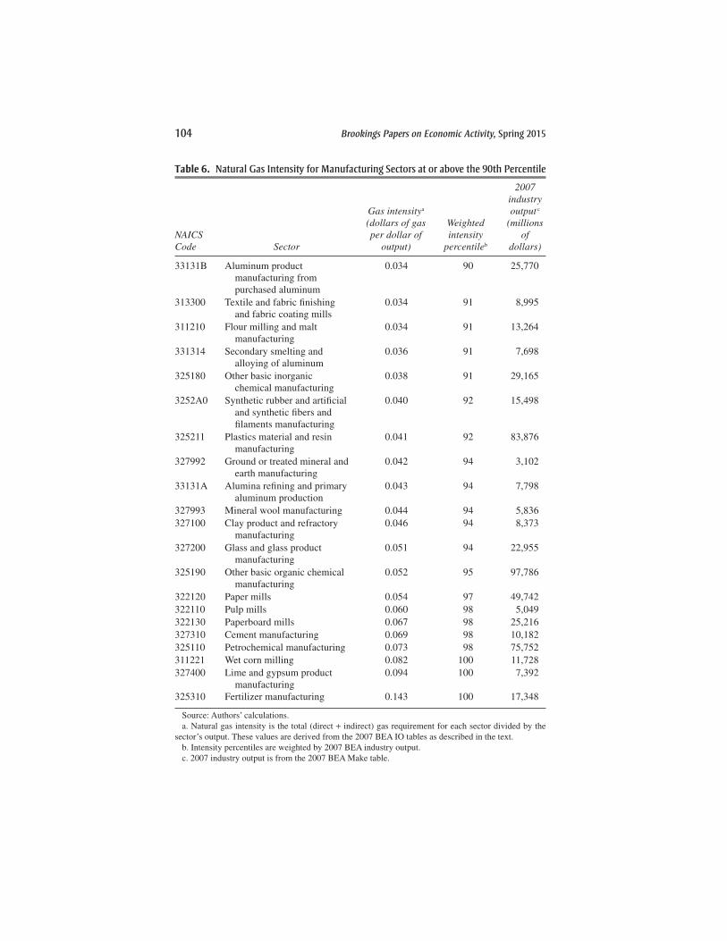
104 Brookings Papers on Economic Activity, Spring 2015
Table 6. Natural Gas Intensity for Manufacturing Sectors at or above the 90th Percentile
NAICS Code Sector
Gas intensitya (dollars of gas per dollar of
output)
Weighted intensity
percentileb
2007 industry output c
(millions of
dollars)
33131B Aluminum product manufacturing from purchased aluminum
0.034 90 25,770
313300 Textile and fabric finishing and fabric coating mills
0.034 91 8,995
311210 Flour milling and malt manufacturing
0.034 91 13,264
331314 Secondary smelting and alloying of aluminum
0.036 91 7,698
325180 Other basic inorganic chemical manufacturing
0.038 91 29,165
3252A0 Synthetic rubber and artificial and synthetic fibers and filaments manufacturing
0.040 92 15,498
325211 Plastics material and resin manufacturing
0.041 92 83,876
327992 Ground or treated mineral and earth manufacturing
0.042 94 3,102
33131A Alumina refining and primary aluminum production
0.043 94 7,798
327993 Mineral wool manufacturing 0.044 94 5,836327100 Clay product and refractory
manufacturing0.046 94 8,373
327200 Glass and glass product manufacturing
0.051 94 22,955
325190 Other basic organic chemical manufacturing
0.052 95 97,786
322120 Paper mills 0.054 97 49,742322110 Pulp mills 0.060 98 5,049322130 Paperboard mills 0.067 98 25,216327310 Cement manufacturing 0.069 98 10,182325110 Petrochemical manufacturing 0.073 98 75,752311221 Wet corn milling 0.082 100 11,728327400 Lime and gypsum product
manufacturing0.094 100 7,392
325310 Fertilizer manufacturing 0.143 100 17,348
Source: Authors’ calculations.a. Natural gas intensity is the total (direct + indirect) gas requirement for each sector divided by the
sector’s output. These values are derived from the 2007 BEA IO tables as described in the text.b. Intensity percentiles are weighted by 2007 BEA industry output.c. 2007 industry output is from the 2007 BEA Make table.

CATHERINE HAUSMAN and RYAN KELLOGG 105
that natural gas is the chemical feedstock for virtually all nitrogen-based fertilizer production (that is, gas is not used merely for process heat).37
Our first analysis of manufacturing sector growth is presented in table 7. This table shows changes in manufacturing establishment counts, employ-ment, employee compensation, and capital expenditure between the 2002 and 2007 Economic Censuses and between the 2007 and 2012 Economic Censuses. We focus our attention on changes from 2007 to 2012, as this was the period during which the shale boom substantially decreased the U.S. natural gas price. Table 7 groups sectors by their manufacturing inten-sity, separately presenting activity changes for sectors below the 90th inten-sity percentile, for sectors above the 90th percentile, for sectors above the 95th percentile, and for fertilizer manufacturing.
The first set of rows in table 7 shows that sectors outside the 90th inten-sity percentile have experienced declining establishment counts, employ-ment, and employee compensation, especially over the 2007–12 period, which includes the Great Recession. The remaining rows show that these
37. Nitrogen-based fertilizers are derived from ammonia (NH3), which is made by com-bining atmospheric nitrogen with hydrogen via the Haber process. Hydrogen is in turn pro-duced via steam reforming of natural gas: reacting natural gas (CH4) with water (H2O) to produce hydrogen (H2) and carbon dioxide (CO2).
Table 7. Changes in Manufacturing Sector Activity: 2002–07 and 2007–12a
Percentages
YearsNumber of
establishments EmploymentEmployee
compensationCapital
expenditure
Sectors with natural gas intensity < 90th percentile2002–07 −5.8 −9.0 9.9 21.32007–12 −10.6 −16.5 −3.7 4.9
Sectors with natural gas intensity ≥ 90th percentile2002–07 −3.5 −14.7 −1.9 36.82007–12 −6.2 −13.1 4.3 8.5
Sectors with natural gas intensity ≥ 95th percentile2002–07 −0.6 −14.3 −1.0 46.52007–12 1.7 −8.6 9.1 2.5
Fertilizer manufacturing (NAICS 325310)2002–07 −9.5 −15.8 8.5 20.42007–12 8.3 8.6 24.8 232.7
Source: Authors’ calculations.a. Manufacturing sector activity data come from the 2002, 2007, and 2012 Economic Censuses (ECs)
and are merged with sector-level natural gas intensity data, as discussed in the text. Percentile classifica-tions of sectors are weighted on 2007 sector output from the BEA.

106 Brookings Papers on Economic Activity, Spring 2015
declines were not as steep for sectors above the 90th and 95th inten-sity percentiles, and that employee compensation actually increased for these sectors. For fertilizer manufacturing, by far the most gas-intensive manufacturing sector, the establishment count, employment, and compen-sation all increased considerably between 2007 and 2012. The change in capital expenditure from 2007 to 2012, while positive for non-gas-intensive sectors, is larger for sectors above the 90th percentile and was a massive 233 percent for fertilizer manufacturing. It is therefore clear that manufac-turing sectors that are particularly gas intensive have expanded relative to other manufacturing sectors since the onset of the shale gas boom.38
Interpreting the changes in gas-intensive manufacturing activity as caused by the shale boom requires us to posit a counterfactual, namely, what would have happened during 2007–12 absent shale gas. One possible counterfactual is that gas-intensive sectors would have experienced the same contraction as did non-gas-intensive sectors. In this case, the effect of shale gas on gas-intensive manufacturing is given by the difference between the 2007 and the 2012 activity changes for intense versus non-intense sectors. Specifically, we find that under this counterfactual shale gas caused sectors above the 90th percentile of gas intensity to experience increases in establishments, employment, compensation, and capital expen-diture of 4.4 percent, 3.4 percent, 8.0 percent, and 3.6 percent, respectively.
An alternative counterfactual is that gas-intensive sectors’ activity changes from 2007 to 2012 would differ from the changes in non-gas-intensive sectors according to the 2002–07 pre-trends. For instance, employment in sectors above the 90th percentile decreased by 5.7 percentage points more than employment in non-gas-intensive sectors between 2002 and 2007, and we might have expected this difference to persist over 2007–12 absent shale gas. Under this counterfactual, the shale boom caused sectors above the 90th intensity percentile to experience increases in establishments, employment, and compensation of 2.2 percent, 9.1 percent, and 19.8 per-cent, respectively, and a decrease in capital expenditure of 11.9 percent (the “triple differenced” capital expenditure effect is positive, however, for fertilizer manufacturing).
38. The establishment count, employment, and compensation changes for 2007–2012 for sectors above the 90th percentile are greater than those for sectors below the 90th percentile even if fertilizer manufacturing is excluded. Establishments, employment, and compensation change by −7.1 percent, −13.7 percent, and 3.8 percent, respectively. Changes relative to the 2002–07 pre-trend are still substantially larger than for non-intense sectors. The change in capital expenditure, however, is relatively small: 2.7 percent.

CATHERINE HAUSMAN and RYAN KELLOGG 107
Overall, this analysis suggests that employment in gas-intensive indus-tries was between 3.4 and 9.1 percent higher in 2012 because of low nat-ural gas prices, a noticeable impact. However, total employment for the industries at or above the 90th percentile of natural gas intensity was only 710,000 in 2013, implying that the number of additional jobs from fracking in those industries was in the range of 24,000 to 65,000.
What about employment impacts for manufacturing sectors outside the 90th percentile? Given that average gas intensity in manufacturing is only 2 percent, we do not expect large percentage changes in employment from the gas price change. It is plausible, however, that even a small percent-age change could imply many additional jobs, when aggregated across all of manufacturing. To analyze this possibility, we estimate the correlation between gas intensity and changes in manufacturing employment from 2007 to 2012. Specifically, we regress log employment by industry in 2012 on gas intensity, controlling for log employment in both 2002 and 2007 and weighting by industry output.39 Conceptually, this regression is similar to the “triple differenced” numbers we report above, but it allows us to study changes within the non-gas-intensive sectors. Including log employment in 2002 and 2007 as explanatory variables is important, since preexisting secular trends in manufacturing activity may be correlated with gas inten-sity. Additionally, we control for three-digit NAICS-code fixed effects to isolate the variation within broad categories of manufacturing.
We estimate a coefficient on gas intensity of 1.3 (with a standard error of 0.8; full regression results are in the online appendix), suggesting that for every additional percentage point of gas intensity, employment in 2012 was 1.3 percent higher. Assuming that a zero-gas-intensity sector would experience no change in employment from the natural gas price fall, we can calculate total employment impacts as follows.
For each sector we multiply the coefficient on gas intensity by the sector’s gas intensity level and by its employment in 2007, yielding the change in the number of jobs in that sector associated with the change in the sector’s natural gas input cost. Summing across sectors, we find an increase in manufacturing employment of around 280,000 in 2012; the 95 percent confidence interval is −60,000 to 610,000. For comparison, total manufacturing employment in 2012 was around 11 million.
39. This regression relies on the employment elasticity with respect to gas prices being proportional to gas share. This proportionality is true for a CES production function and constant elasticity demand.

108 Brookings Papers on Economic Activity, Spring 2015
Overall, while it is difficult to pinpoint a precise causal effect, the bal-ance of the evidence suggests that manufacturing has experienced an expansion of activity as a result of the shale boom. The total employment effect would, of course, depend on whether new jobs in manufacturing were moved from other sectors (a multiplier less than one) or whether this growth contributed to employment in other sectors (a multiplier greater than one). In addition, the 2007–12 time period we study may be too brief to observe the full long-run effect of lower natural gas prices on manufac-turing employment: slow-moving investments in capital may need to be completed before the full employment effects are realized.40
We conclude this section by studying prices for two gas-intensive chem-ical products for which data are readily available: ammonia, a major fer-tilizer and the precursor to nearly all other nitrogen-based fertilizers, and high-density polyethylene, a common type of plastic. Ammonia is manu-factured using methane, the primary chemical component of natural gas, as a direct input. High-density polyethylene can be produced using ethane, the second most common component of natural gas, as a feedstock (with ethylene as a crucial intermediate product).41 These two products are inter-esting because, relative to their natural gas inputs, their international trans-portation costs are low. Whereas methane has a boiling point of −161°C and ethane has a boiling point of −89°C, ammonia boils at −33°C and high-density polyethylene is a solid at room temperature, facilitating the shipment of these two products.
The ease of trade for ammonia and high-density polyethylene leads to international parity in their prices. The upper panel of figure 8 presents time series of ammonia prices for the U.S. Gulf Coast, the Black Sea, and the Middle East. The figure makes clear that ammonia prices in these three regions are tightly linked despite large overall price fluctuations. In par-ticular, the U.S. ammonia price does not substantially diverge from Black Sea and Middle East prices after 2007, despite the large decrease in the U.S. natural gas price. The lower panel of figure 8 shows a similar result for high-density polyethylene and its input, ethane.42 The U.S. and Western
40. We have estimated the regression described above using investment as the dependent variable rather than employment. The estimation results are very sensitive to the inclusion or exclusion of the fertilizer sector.
41. High-density polyethylene can also be produced through the processing of crude oil, where the long-chain hydrocarbons in crude can be “cracked” to produce ethylene.
42. The U.S. ethane prices are FOB contract prices, and the Western Europe ethane prices are derived by Nexant. We obtain both series from Bloomberg.

CATHERINE HAUSMAN and RYAN KELLOGG 109
Figure 8. Ammonia, Ethane, and High-Density Polyethylene Prices, U.S. and International, 2006–14
3
6
9
12
15
U.S. Henry Hub gas price,$/mcf
200
400
600
800
1,000
Ammonia price, U.S. dollars per metric ton
July 2006 July 2008 July 2010 July 2012 July 2014
U.S. Gulf Coast
Black Sea
Middle East
Henry Hub gas
Ammonia vs. natural gas
Ethane price,U.S. dollars per metric ton
HDPE price, U.S. dollars per metric ton
HDPE vs. ethane
200
400
600
800
1,000
500
1,000
1,500
2,000
2,500
July 2006 July 2008 July 2010 July 2012 July 2014
HDPE, U.S.A.
HDPE, Western Europe
Ethane, U.S.A.
Ethane, Western Europe
Source: Bloomberg.
110 Brookings Papers on Economic Activity, Spring 2015
European prices for high-density polyethylene follow each other closely, even though the U.S. ethane price has fallen far below ethane prices in Western Europe. The lack of pass-through of U.S. natural gas prices to ammonia and HDPE prices implies that the welfare gains for these sectors caused by cheap natural gas are accruing almost entirely to manufacturers rather than consumers.
The divergence between U.S. ammonia and natural gas prices also helps to explain the tremendous expansion of U.S. fertilizer manufacturing shown in table 7 above. Because ammonia prices are set on a large global market, U.S. fertilizer manufacturers are able to expand their production without substantially affecting their output price. While we lack sector-specific employment and production data for high-density polyethylene, the EIA reports that several firms have now planned substantial investments in chemical plants that will use ethane to produce ethylene, a key ingredi-ent for this and other plastics (EIA 2015). This new capacity—driven by low U.S. feedstock prices relative to prices elsewhere—is expected to increase ethylene production by 40 percent once it comes online in 2017 or 2018 (EIA 2015).
VI. Environmental Externalities and Regulation
Scientists have identified a number of potential environmental impacts from fracking, although much research is still needed. Below we briefly summarize the concerns brought forward to date. We then discuss how the existing environmental economics literature might shed light on the options available to regulators.
VI.A. Global Environmental Impacts
Fracking could affect climate change through several mechanisms, and overall the impact could be to either decrease or increase total greenhouse gas emissions (McJeon and others 2014, Newell and Raimi 2014). First, methane leaks can occur throughout the natural gas production chain, and methane is a powerful greenhouse gas. The rate at which methane is leak-ing from the supply chain is much debated (Moore and others 2014), in part because the leak rate is very heterogeneous across producers and sites (Brandt and others 2014). Below we discuss how this uncertainty affects the optimal regulatory approach.
The second way fracking could impact climate change is through the combustion of natural gas as fuel. Two effects operate here: one is the lower price of natural gas encouraging total energy use to rise (a scale effect), and the other is the lower price encouraging substitution away from other
CATHERINE HAUSMAN and RYAN KELLOGG 111
fuels, both less carbon-intensive ones (renewables and nuclear) and those that are more carbon-intensive (coal and oil). According to simulations by Richard Newell and Daniel Raimi (2014), the coal displacement effect has dominated both the scale effect and the effect on renewables and nuclear use, so that domestic emissions from combustion have decreased. After incorporating the effect of methane leaks, however, their results for overall domestic greenhouse gas emissions are inconclusive. Moreover, the total global impact depends on whether and by how much coal exports have increased. Newell and Raimi (2014) suggest that the coal export effect is small, but more research on the global coal market is needed to definitively answer this question.
To illustrate the wide variation in potential climate impacts, consider two bounding scenarios.43 First, suppose that all displaced coal is exported and international coal production is not reduced at all (this is an extreme bound, both because some displaced coal is likely not extracted and because some international coal production is reduced). In this case, there are no substitu-tion benefits, and CO2 emissions increase from the scale effect. In this case, CO2 emissions would have increased by 340 million tons in 2013 because of fracking. Applying the social cost of carbon as calculated by the Inter-agency Working Group on the Social Cost of Carbon,44 which is $40 a ton, this would be worth $13 billion a year.
Additionally, applying the highest estimate of the methane leak rate in the recent literature (7.9 percent), methane emissions from fracking would have increased from 2007 to 2013 by 11 million tons; with a global warm-ing potential of 34, this would be worth an additional $15 billion per year.45
At the other extreme of possible scenarios, consider the case in which the increase in gas-fired electricity generation has displaced coal with no offsetting increase in exports (or equivalently, assume any increase in coal exports was completely offset by reductions in coal production abroad). In this lower-bound case, CO2 emissions from electricity production would have decreased by 70 million tons in 2013 because of fracking, implying a savings of $2.8 billion per year. Residential, commercial, and industrial sector emissions, however, still would have increased by almost 130 million tons due to the scale effect, for a cost of $5.3 billion per year. Overall, in this lower bound case, fracking would have led to a cost of $2.5 billion per
43. Parameter assumptions and calculations are given in the online appendix.44. IWG: Interagency Working Group on the Social Cost of Carbon, United States
Government. See the online appendix for details.45. Methane’s global warming potential of 34 means that each ton of methane in the
atmosphere would trap as much heat as 34 tons of CO2.

112 Brookings Papers on Economic Activity, Spring 2015
year from increased CO2 emissions. Newell and Raimi (2014) find that the coal displacement effect dominates the scale effect, a function of different demand elasticities.46 For a lower bounding case for methane leaks, a leak rate of 0.42 percent would imply an increase in methane emissions of 0.5 million tons, worth $0.5 billion per year.
Overall, then, our bounding exercise suggests that the climate-change impact of fracking in 2013 could have been an increase in environmen-tal costs of anywhere from $3.0 billion a year to $28 billion a year, at a social cost of carbon of $40 a ton. Some of this range is from uncertainty regarding coal displacement, and some is from uncertainty over methane leaks. An additional caveat is important and points to the need for further research. The long-run impact of low natural gas prices on the transition to a less carbon intensive energy sector depends crucially on how the prices affect investment decisions (for new power plants, the vehicle fleet, and so on) as well as future expenditures on research and development. Existing models, such as the EIA’s National Energy Modeling System model, incor-porate investment decisions, but impacts on research and development are largely unknown. Although technology has advanced for renewable energy sources such as solar and wind, it is worth highlighting that the pace of technological advances for oil and gas extraction in recent years has been astounding. In the absence of climate policy, renewables must advance technologically faster than fossil fuels in order to displace them.
VI.B. Local Environmental Impacts
The environmental impact that has perhaps attracted the most attention to date is the potential for water contamination. Contamination can occur at several stages of the extraction process, affecting either surface water or groundwater. Damages can result from the natural gas itself, the toxic fluids used in the fracking process, or other naturally occurring chemicals released by the fracking process (Burton, Nadelhoffer, and Presley 2013). Concern has also been raised about the volume of water used for frack-ing and the resulting potential for surface or groundwater depletion. For a review of studies analyzing the risks to water, see Robert Jackson and others (2014), Mason, Muehlenbachs, and Olmstead (2014), and Mitchell Small and others (2014); the EPA is also currently undertaking a large-scale review of water impacts (EPA, 2011).
46. The demand elasticities in Newell and Raimi (2014), all taken from the EIA’s NEMS model, are in the range of −0.1 to −0.5 for the residential, commercial, and industrial sectors, but the elasticity for the electric power sector is substantially larger.

CATHERINE HAUSMAN and RYAN KELLOGG 113
A second area of concern relates to local air quality. Emissions of both criteria and toxic pollutants could again result from several components of the extraction process, including the well itself, compressor stations, and transport equipment (Mason, Muehlenbachs, and Olmstead 2014, Moore and others 2014). On the other hand, increased natural gas production may lead to air quality improvements to the extent that it causes displacement of coal in electric power generation and therefore reductions in pollutants such SO2, NOx, particulate matter, and mercury.
Unconventional gas extraction also involves a great deal of transport equipment. In addition to creating road dust, the increased trucking can lead to increased traffic accidents and fatalities (Graham and others 2015). The heavy truck traffic may also cause significant damage to local roads; Shmuel Abramzon and others (2014) provide estimates of roadway dam-ages for the Marcellus shale in Pennsylvania.
Additionally, scientists have pointed to earthquakes associated with the injection of wastewater in fracking operations (EPA 2014; Small and others 2014). Comprehensive analysis of this seismic activity is still lacking. As with conventional oil and gas extraction activity, habitat frag-mentation can also occur, and studies specific to the areas being newly developed for unconventional gas are still limited (Small and others 2014, Mason, Muehlenbachs, and Olmstead 2014). The final local external-ity that has raised concern is the suite of disamenities associated with a rapidly growing “boomtown,” including noise and crime. Overall, the empirical evidence on these disamenities is mixed (Jacquet 2014, Mason, Muehlenbachs, and Olmstead 2014, Raimi and Newell 2014), but they may well be large in some regions. Finally, one recent study has found an impact of drilling on infant health in Pennsylvania, but the precise mecha-nism is unknown (Hill 2013).
Overall, a number of local environmental impacts have been identified, and site-specific studies are accumulating. A valuable complement to our consumer and producer surplus calculations would be a full monetization of these impacts. Unfortunately, that is not yet possible given the state of the data on water and air quality. Even two recent federal rules on frack-ing failed to monetize environmental impacts.47 Mason, Muehlenbachs, and
47. These are (i) the Bureau of Land Management (BLM) regulation published in the Federal Register, vol. 80, no. 58, “Oil and Gas; Hydraulic Fracturing on Federal and Indian Lands; Final Rule,” March 26, 2015; and (ii) the Environmental Protection Agency (EPA) regulation published in the Federal Register, vol. 77, no. 159, “Oil and Natural Gas Sector: New Source Performance Standards and National Emission Standards for Hazardous Air Pollutants Reviews; Final Rule,” August 16, 2012.

114 Brookings Papers on Economic Activity, Spring 2015
Olmstead (2014) summarize the limited damages estimated in the literature to date. For all of the impacts, more analysis is still needed on their mag-nitude and geographic scope (Mason, Muehlenbachs, and Olmstead 2014; Small and others 2014). Only with improved physical data on impacts will it be possible to obtain a comprehensive bottom-up economic valuation of the local environmental effects of fracking, using marginal damage esti-mates such as those developed by Nicholas Muller and Robert Mendelsohn (2009) for local air pollutants.
An alternative, top-down approach to local environmental impact eval-uation would be to focus on housing prices, as in Lucija Muehlenbachs, Elisheba Spiller, and Christopher Timmins (2012, 2014). In theory, home values can fully capitalize the value of all local environmental disameni-ties to the marginal resident. However, interpretation of results on housing prices is difficult for several reasons. First, the change in housing prices reflects not only environmental disamenities but also the local boom in economic activity and resource rents associated with extraction. Second, responses of housing prices to changes in disamenities do not in general reveal marginal valuations or welfare changes when households have het-erogeneous preferences (Kuminoff and Pope forthcoming; Haninger, Ma, and Timmins 2014). Finally, if information on environmental impacts is incomplete, the values of the homes reflect only the perceived level of environmental disamenities. This last issue is particularly important in the context of fracking, where the extent of and spatial heterogeneity in dam-ages remains unknown.
VII. Regulatory Approaches
Environmental regulation of fracking varies considerably across locations (Richardson and others 2013), but in general, comprehensive and cost-effective environmental regulation has lagged behind the rapid rise of unconventional natural gas. At the federal level, regarding the two recent rules mentioned above, the 2012 EPA rule regulates some forms of air emissions but not others, and the 2015 BLM rule only applies to federal lands (see note 47). Additionally, while some states and localities have banned fracking outright, other areas have allowed the industry to rapidly move forward. From an efficiency perspective, this variation in policy approaches is unlikely to be optimal.
Several factors have impeded the development of unified and cost-effective regulation. As the previous discussion made clear, a great deal of

CATHERINE HAUSMAN and RYAN KELLOGG 115
uncertainty still surrounds the location and extent of the damages outlined. The damages are likely to be heterogeneous across space; for instance, groundwater contamination and methane leaks both depend on the integrity of equipment (Allen and others 2013; Ingraffea and others 2014) and will therefore vary across producers and sites. This heterogeneity affects the ability of the scientific community to estimate the magnitude of the overall problem; it also limits the ability of policymakers to rapidly target the envi-ronmental impacts of greatest concern.
It is worth considering fracking in the light of other environmental prob-lems characterized by uncertainty and lack of data. In particular, we will highlight both poor monitoring and difficult attribution of liability. We begin by discussing examples of uncertainty about environmental damages from fracking; then we discuss implications for regulators.
To hold individual producers accountable for the damages they cause, regulators must (i) observe a baseline level of environmental quality; (ii) document a change in environmental quality from fracking; and (iii) attribute the change directly to an individual producer. The first problem to date, then, has been lack of complete data on baseline envi-ronmental quality levels for surface water, groundwater, and air qual-ity (Adgate, Goldstein, and McKenzie 2014, Burton, Nadelhoffer, and Presley 2013, Moore and others 2014, Small and others 2014). Even in locations where baseline and post-fracking water quality have been measured, it remains difficult to hold individual producers liable (Davis 2015). As Fitzgerald (2013) points out, “Fracking occurs far under-ground, where verification is costly if not impossible” (p. 1356). Con-tamination occurs if wells are poorly encased (Darrah and others 2014, Fitzgerald 2013, Ingraffea and others 2014, Vidic and others 2013), but monitoring every individual well is costly (Davis 2015). Researchers have found that incomplete data on well casing integrity poses a real challenge (Jackson and others 2014).
Comprehensive monitoring and attribution of methane emissions is also difficult. Methane can be emitted from a number of sources throughout the extraction process; for a description, see David Allen and others (2013) and Christopher Moore and others (2014). Direct measurement of most of the individual sources is possible, but such measurements to date have been limited to snapshots taken at a small sample of sites (Allen and others 2013, Brandt and others 2014). An alternative is to measure the entire plume at a downwind location, so that only one measurement is needed. However, a suitable downwind location is not available at all sites (Allen

116 Brookings Papers on Economic Activity, Spring 2015
and others 2013); moreover, a regulator must then prove that all of the observed emissions are from a given producer, rather than other nearby sources. The EPA has struggled with similar difficulties in other industries, such as refining.48
Cost-effective regulation is extremely challenging in settings with incom-plete data and imperfect attribution. The standard market-based incentives that economists prefer, such as emissions taxes or cap-and-trade programs, can only be used with high-quality monitoring. The efficiency of these incentives is predicated on rewarding the firms that engage in clean produc-tion while punishing firms that emit—and clearly, this requires attribution to individual firms.
In the absence of market-based incentives, two broad types of regula-tory approaches are currently in place (in addition to outright bans and moratoriums). The first is holding producers liable for accidents after the fact through the judicial system. This again requires proof of damages, so the data quality and attribution issues discussed above still apply. More-over, incentives for emissions abatement can be greatly distorted when penalties are applied through the tort system (Davis 2015). As an example, bankruptcy protection will exempt very small firms from ex-post liability of large accidents (Boomhower 2014).
The second regulatory approach currently in place is command-and-control regulation, mainly through technology standards. For instance, individual state environmental agencies have imposed a suite of stan-dards on well casing, well depth, wastewater storage, and similar elements (Richardson and others 2013). One well-known problem with relying on technology standards is that implementation may vary considerably across firms. For this industry, many firms are engaged in extraction of unconven-tional natural gas, and they are of varying sizes and degrees of technical capability (Small and others 2014). Moreover, with technology standards, the regulator will not necessarily observe whether the technology is cor-rectly installed. This issue is important for both methane leaks and well casings, which are a function of equipment integrity.
The academic literature in environmental economics has proposed a set of regulations that are incentive-compatible even under imperfect attribution. First proposed by Kathleen Segerson (1988), the approach
48. See, for instance, Federal Register, vol. 79, no. 125, “Petroleum Refinery Sector Risk and Technology Review and New Source Performance Standards; Proposed Rule,” June 30 2014; http://www.gpo.gov/fdsys/pkg/FR-2014-06-30/pdf/2014-12167.pdf

CATHERINE HAUSMAN and RYAN KELLOGG 117
combines ambient environmental quality standards with joint liability. For instance, if regulators can observe groundwater quality throughout a geographic area, they hold all firms in that area liable for any damages to the water. Not surprisingly, despite a large theoretical literature, legal and political barriers have prevented this approach from being implemented.
One could imagine, however, a version of the Segerson (1988) approach being applied to unconventional natural gas extraction. This variant allows firms to opt out of the penalties if they can prove, with their own (regulator-verified) monitoring devices, that they did not contribute to the damages (Millock, Sunding, and Zilberman 2002).49 This approach leverages self-selection of clean firms into self-monitoring. One could imagine clean, technologically advanced firms agreeing to this sort of solution for ground-water emissions, surface water emissions, and methane leaks in order to prevent a total ban on fracking activities.
In conclusion, scientists remain concerned about a number of environ-mental damages caused by fracking. Unfortunately, data collection has not kept pace with the boom in extraction, and a great deal of uncertainty remains regarding pollution from fracking. This uncertainty has limited the ability of regulators to target those areas of greatest concern; it has also limited their ability to regulate in a cost-effective way. Higher quality, comprehensive data on baseline levels of environmental quality as well as on emissions from individual producers would go a long way. In the absence of such data, regulatory options remain limited and are unlikely to be cost-effective.
VIII. Conclusion
This paper provides what we believe to be the most comprehensive analy-sis to date of how shale gas development has affected the welfare of U.S. natural gas consumers—including both households and industries—as well as producers of natural gas. We estimate both the demand and supply curves for natural gas and then use these estimates to find that the expan-sion of natural gas supply reduced U.S. natural gas prices between 2007 and 2013 by $3.45 per mcf, equivalent to 47 percent of the counterfactual 2013 price. This price reduction has led to large increases in surplus for natural gas purchasers, particularly in the South Central and Midwestern
49. Recently enacted legislation in North Carolina does involve presumptive liability for water contamination, placing the burden of proof on the gas developer or operator.

118 Brookings Papers on Economic Activity, Spring 2015
United States, where the industrial and electric power sectors consume large quantities of gas.
We confirm that the wholesale natural gas price reduction has fully passed through to retail rates for all sectors. However, pass-through of industrial gas prices to prices for gas-intensive manufactured products need not be 100 percent. For ammonia and high-density polyethylene, two commodity chemicals with gas-intensive production processes, we show that U.S. and international output prices are tightly linked even though natural gas input prices have diverged, suggesting that pass-through is very small.
In contrast to natural gas purchasers, we find that natural gas produc-ers have experienced a reduction in surplus because their gain from the expansion of supply has been outweighed by the fall in the gas price. These surplus reductions are particularly acute in regions that have historically produced large quantities of conventional natural gas but have not devel-oped shale resources. Combining our consumer and producer surplus estimates, we estimate that the shale boom increased total U.S. consumer-plus-producer surplus by $48 billion in 2013. Under plausible alternative assumptions, this number varies by up to 20 percent. Future gains could be larger through long-run capital replacement and innovation effects, par-ticularly on the demand side. Currently planned levels of LNG exports will further increase U.S. total surplus, but the gains will be modest because the increase in producer surplus will be shared with Canadian exporters to the United States.
Importantly, our consumer and producer surplus estimates omit changes in welfare associated with environmental externalities from shale gas development. We provide a summary of the potential local and global envi-ronmental impacts from the fracking revolution, noting that for the vast majority of these impacts the data necessary to obtain an economic valua-tion do not exist. We identify plausible bounds on the increase in external costs from climate impacts for 2013 that range from $3.0 billion to $28 bil-lion, though other studies have found that climate impacts may actually be beneficial (McJeon and others 2014, Newell and Raimi 2014). Bounding the economic value of all local impacts is not currently possible, and the aggregate impact may be positive or negative. It is therefore impossible to know, at present, the extent to which environmental externalities affect the net welfare gains to natural gas consumers and producers. Improvements in data collection would be immensely valuable both for quantifying poten-tial environmental impacts from fracking and for enabling cost-effective regulation.

CATHERINE HAUSMAN and RYAN KELLOGG 119
ACKNOWLEDGMENTS We thank Steve Cicala, David Lagakos, and the editors for valuable comments; Karen Fisher-Vanden, Timothy Fitzgerald, Laura Grant, Joshua Hausman, Kelsey Jack, Lutz Kilian, Cathy Kling, Tom Lyon, Lucija Muehlenbachs, Yueming Qiu, Barry Rabe, and Daniel Raimi for helpful feedback; and Sarah Johnston for excellent research assistance.

120 Brookings Papers on Economic Activity, Spring 2015
References
Abramzon, Shmuel, Constantine Samaras, Aimee Curtright, Aviva Litovitz, and Nicholas Burger. 2014. “Estimating the Consumptive Use Costs of Shale Nat-ural Gas Extraction on Pennsylvania Roadways.” Journal of Infrastructure Systems 20, no. 3.
Adgate, John L., Bernard D. Goldstein, and Lisa M. McKenzie. 2014. “Potential Public Health Hazards, Exposures and Health Effects from Unconventional Natural Gas Development.” Environmental Science and Technology 48, no. 15: 8307–20.
Agerton, Mark, Peter Hartley, Kenneth B. Medlock III, and Ted Temzelides. 2015. “Employment Impacts of Upstream Oil and Gas Investment in the United States.” Working Paper no. 15/28. Washington: International Monetary Fund.
Allcott, Hunt, and Daniel Keniston. 2014. “Dutch Disease or Agglomeration? The Local Economic Effects of Natural Resource Booms in Modern America.” NBER Working Paper no. 20508. Cambridge, Mass.: National Bureau of Economic Research.
Allen, David T., Vincent M. Torres, James Thomas, David W. Sullivan, Matthew Harrison, Al Hendler, Scott C. Herndon, Charles E. Kolb, Matthew P. Fraser, A. Daniel Hill, Brian K. Lamb, Jennifer Miskimins, Robert F. Sawyer, and John H. Seinfeld. 2013. “Measurements of Methane Emissions at Natural Gas Production Sites in the United States.” Proceedings of the National Academy of Sciences 110, no. 44: 17768–73.
Anderson, Soren T., Ryan Kellogg, and Stephen W. Salant. 2014. “Hotelling under Pressure.” NBER Working Paper no. 20280. Cambridge, Mass.: National Bureau of Economic Research.
Arora, Vipin. 2014. “Estimates of the Price Elasticities of Natural Gas Supply and Demand in the United States.” Munich Personal RePEc Archive (MPRA) Paper No. 54232. http://mpra.ub.uni-muenchen.de/54232/1/MPRA_paper_54232.pdf
Arora, Vipin, and Yiyong Cai. 2014. “U.S. Natural Gas Exports and Their Global Impacts.” Applied Energy 120, no. 1: 95-103.
Boomhower, Judson. 2014. “Drilling Like There’s No Tomorrow: Bankruptcy, Insurance, and Environmental Risk.” Working Paper no. 254, Energy Institute at Haas, University of California at Berkeley. https://ei.haas.berkeley.edu/ research/papers/WP254.pdf#page=1
Borenstein, Severin, and Ryan Kellogg. 2014. “The Incidence of an Oil Glut: Who Benefits from Cheap Crude Oil in the Midwest?” Energy Journal 35, no. 1: 15–33.
Brandt, A. R., G. A. Heath, E. A. Kort, F. O’Sullivan, and others. 2014. “Methane Leaks from North American Natural Gas Systems.” Science 343, no. 6172: 733–35.
Brehm, Paul. 2015. “Natural Gas Prices, Electric Generation Investment, and Greenhouse Gas Emissions.” Working Paper. http://www-personal.umich.edu/ ∼pabrehm/Gas%20Prices%20and%20Emissions.pdf
Brown, Jason P., Timothy Fitzgerald, and Jeremy G. Weber. 2015. “Capturing Rents from Natural Resource Abundance: Private Royalties from U.S. Onshore

CATHERINE HAUSMAN and RYAN KELLOGG 121
Oil and Gas Production.” Research Working Paper no. 15-04, Federal Reserve Bank of Kansas City.
Brown, Stephen P. A., and Alan J. Krupnick. 2010. “Abundant Shale Gas Resources: Long-Term Implications for U.S. Natural Gas Markets.” RFF Discussion Paper no. 10-41. Washington: Resources for the Future.
Brown, Stephen P. A., Charles Mason, Alan Krupnick, and Jan Mares. 2014. “Crude Behavior: How Lifting the Export Ban Reduces Gasoline Prices in the United States.” RFF Issue Brief 14-03-REV. Washington: Resources for the Future.
Burton, G. Allen, Knute J. Nadelhoffer, and Kathleen Presley. 2013. “Environment/ Ecology Technical Report: Hydraulic Fracturing in the State of Michigan.” Integrated Assessment Report Series 2, no. 4. Ann Arbor, Michigan: Graham Sustainability Institute.
Congressional Budget Office (CBO). 2014. “The Economic and Budgetary Effects of Producing Oil and Natural Gas from Shale.” Washington.
Credit Suisse. 2012. “US Natural Gas Reservoir: Conventional Wisdom.” Securi-ties Research & Analytics (online). June 6.
Cullen, Joseph A., and Erin T. Mansur. 2014. “Inferring Carbon Abatement Costs in Electricity Markets: A Revealed Preference Approach Using the Shale Rev-olution.” Working Paper no. 20795. Cambridge, Mass.: National Bureau of Economic Research.
Darrah, Thomas H., Avner Vengosh, Robert B. Jackson, Nathaniel R. Warner, and Robert J. Poreda. 2014. “Noble Gases Identify the Mechanisms of Fugi-tive Gas Contamination in Drinking-Water Wells Overlying the Marcellus and Barnett Shales.” Proceedings of the National Academy of Sciences 111, no. 39: 14076–81.
Davis, Lucas. 2015. “Bonding Requirements for U.S. Natural Gas Producers.” Review of Environmental Economics and Policy 9, no. 1: 128–144.
Davis, Lucas, and Catherine Hausman. 2015. “Market Impacts of a Nuclear Power Plant Closure.” Working Paper no. 248R, Energy Institute at Haas, University of California at Berkeley. https://ei.haas.berkeley.edu/research/papers/WP248R.pdf
Davis, Lucas W., and Erich Muehlegger. 2010. “Do Americans Consume Too Little Natural Gas? An Empirical Test of Marginal Cost Pricing.” RAND Journal of Economics 41, no. 4: 791–810.
DeLeire, Thomas, Paul Eliason, and Christopher Timmins. 2014. “Measuring the Employment Impacts of Shale Gas Development.” Working Paper. http://www.iza.org/conference_files/EnvEmpl2014/timmins_c10226.pdf
Energy Information Administration (EIA). 2014. “Effect of Increased Levels of Liquefied Natural Gas Exports on U.S. Energy Markets.” Washington: U.S. Department of Energy.
———. 2015. “Growing U.S. HGL Production Spurs Petrochemical Industry Investment.” Washington: U.S. Department of Energy.

122 Brookings Papers on Economic Activity, Spring 2015
Environmental Protection Agency (EPA). 2011. “Plan to Study the Potential Impacts of Hydraulic Fracturing on Drinking Water Resources.” http://water.epa.gov/type/groundwater/uic/class2/hydraulicfracturing/upload/hf_study_plan_ 110211_final_508.pdf
———. 2014. “Minimizing and Managing Potential Impacts of Injection-Induced Seismicity from Class II Disposal Wells: Practical Approaches.” http://www2.epa.gov/sites/production/files/2015-08/documents/induced-seismicity-201502.pdf
Federal Energy Regulatory Commission (FERC). 2015a. “North American LNG Export Terminals Proposed.” http://www.ferc.gov/industries/gas/indus-act/lng/lng-export-proposed.pdf.
———. 2015b. “North American LNG Import/Export Terminals Approved.” http://www.ferc.gov/industries/gas/indus-act/lng/lng-proposed-export.pdf
Fitzgerald, Timothy. 2013. “Frackonomics: Some Economics of Hydraulic Fractur-ing.” Case Western Reserve Law Review 63, no. 4: 1337–62.
Graham, Jove, Jennifer Irving, Xiaoqin Tang, Stephen Sellers, Joshua Crisp, Daniel Horwitz, Lucija Muehlenbachs, Alan Krupnick, and David Carey. 2015. “Increased Traffic Accident Rates Associated With Shale Gas Drilling in Pennsylvania.” Accident Analysis and Prevention 74: 203–09.
Hamilton, James D. 2009. “Causes and Consequences of the Oil Shock of 2007–08.” Brookings Papers on Economic Activity, Spring: 215–61.
———. 2011. “Nonlinearities and the Macroeconomic Effects of Oil Prices.” Macroeconomic Dynamics 15 (Supplement S3): 364–78.
Haninger, Kevin, Lala Ma, and Christopher Timmins. 2014. “The Value of Brown-field Remediation.” NBER Working Paper no. 20296. Cambridge, Mass.: National Bureau of Economic Research.
Hill, Elaine L. 2013. “Shale Gas Development and Infant Health: Evidence from Pennsylvania.” Working Paper no. 2012-12, Charles H. Dyson School of Applied Economics and Management, Cornell University.
Holladay, J. Scott, and Jacob LaRiviere. 2014. “The Impact of Cheap Natural Gas on Marginal Emissions from Electricity Generation and Implications for Energy Policy.” Working Paper. http://web.utk.edu/∼jhollad3/Abundant_Gas.pdf
Howarth, Robert W. 2014. “A Bridge to Nowhere: Methane Emissions and the Greenhouse Gas Footprint of Natural Gas.” Energy Science and Engineering 2, no. 2: 47–60.
Ingraffea, Anthony R., Martin T. Wells, Renee L. Santoro, and Seth B. C. Shonkoff. 2014. “Assessment and Risk Analysis of Casing and Cement Impairment in Oil and Gas Wells in Pennsylvania, 2000–12.” Proceedings of the National Acad-emy of Sciences 111, no. 30: 10955–60.
Jackson, Robert B., Avner Vengosh, J. William Carey, Richard J. Davies, Thomas H. Darrah, Francis O’Sullivan, and Gabrielle Petron. 2014. “The Environmental

CATHERINE HAUSMAN and RYAN KELLOGG 123
Costs and Benefits of Fracking.” Annual Review of Environment and Resources 39: 327–62.
Jacquet, Jeffrey B. 2014. “Review of Risks to Communities from Shale Energy Development.” Environmental Science and Technology 48, no. 15: 8321–33.
Kilian, Lutz. 2009. “Not All Oil Price Shocks Are Alike: Disentangling Demand and Supply Shocks in the Crude Oil Market.” American Economic Review 99, no. 3: 1053–69.
———. 2014a. “The Impact of the Shale Oil Revolution on U.S. Oil and Gasoline Prices.” Working Paper no. 499. Frankfurt, Germany: Center for Financial Studies.
———. 2014b. “Oil Price Shocks: Causes and Consequences.” Annual Review of Resource Economics 6: 133–54.
Kilian, Lutz, and Daniel P. Murphy. 2014. “The Role of Inventories and Specula-tive Trading in the Global Market for Crude Oil.” Journal of Applied Econo-metrics 29, no. 3: 454–78.
Knittel, Christopher R., Konstantinos Metaxoglou, and Andre Trindade. 2014. “Dash for Gas: The Sequel.” Working Paper. http://web.mit.edu/knittel/www/papers/Coal_latest.pdf
Krupnick, Alan J., Raymond J. Kopp, Kristin Hayes, and Skyler Roeshot. 2014. “The Natural Gas Revolution: Critical Questions for a Sustainable Energy Future.” http://www.rff.org/files/sharepoint/WorkImages/Download/RFF-Rpt-NaturalGasRevolution.pdf.
Krupnick, Alan J., Zhongmin Wang, and Yushuang Wang. 2013. “Sector Effects of the Shale Gas Revolution in the United States.” RFF Discussion Paper no. 13-20. Washington: Resources for the Future.
Kuminoff, Nicolai V., and Jaren C. Pope. 2014. “Do ‘Capitalization Effects’ for Public Goods Reveal the Public’s Willingness to Pay?” International Eco-nomic Review 55, no. 4: 1227–50.
Linn, Joshua, Lucija Muehlenbachs, and Yushuang Wang. 2014. “How Do Natural Gas Prices Affect Electricity Consumers and the Environment?” RFF Discus-sion Paper no. 14-19. Washington: Resources for the Future.
Maniloff, Peter, and Ralph Mastromonaco. 2015. “The Local Economic Impacts of Fracking.” Working Paper. http://pages.uoregon.edu/ralphm/fracking_may_15.pdf
Mason, C., Lucija Muehlenbachs, and Sheila Olmstead. 2014. “The Economics of Shale Gas Development.” RFF Discussion Paper no. 14-42-REV. Washington: Resources for the Future.
McJeon, Haewon, Jae Edmonds, Nico Bauer, Leon Clarke, Brian Fisher, Brian P. Flannery, Jerome Hilaire, Volker Krey, Giacomo Marangoni, Raymond Mi, Keywan Riahi, Holger Rogner, and Massimo Tavoni. 2014. “Limited Impact on Decadal-Scale Climate Change from Increased Use of Natural Gas.” Nature 514, no. 7523: 482–5.

124 Brookings Papers on Economic Activity, Spring 2015
Melick, William R. 2014. “The Energy Boom and Manufacturing in the United States.” International Finance Discussion Paper no. 1108. Washington: Board of Governors of the Federal Reserve System.
Millock, Katrin, David Sunding, and David Zilberman. 2002. “Regulating Pollu-tion with Endogenous Monitoring.” Journal of Environmental Economics and Management 44, no. 2: 221–41.
Moore, Christopher W., Barbara Zielinska, Gabrielle Petron, and Robert B. Jackson. 2014. “Air Impacts of Increased Natural Gas Acquisition, Process-ing, and Use: A Critical Review.” Environmental Science and Technology 48, no. 15: 8349–59.
Muehlenbachs, Lucija, Elisheba Spiller, and Christopher Timmins. 2012. “Shale Gas Development and Property Values: Differences across Drinking Water Sources.” Working Paper no. 18390. Cambridge, Mass.: National Bureau of Economic Research.
———. 2014. “The Housing Market Impacts of Shale Gas Development.” Working Paper no. 19796. Cambridge, Mass.: National Bureau of Economic Research.
Muller, Nicholas Z., and Robert Mendelsohn. 2009. “Efficient Pollution Regulation: Getting the Prices Right.” American Economic Review 99, no. 5: 1714–39.
National Economic Research Associates (NERA). 2014. “Updated Macro economic Impacts of LNG Exports from the United States.” http://www.nera.com/ content/dam/nera/publications/archive2/PUB LNG Update 0214 FINAL.pdf
Newell, Richard G., and Daniel Raimi. 2014. “Implications of Shale Gas Develop-ment for Climate Change.” Environmental Science and Technology 48, no. 15: 8360–8.
Paredes, Dusan, Timothy Komarek, and Scott Loveridge. 2015. “Income and Employment Effects of Shale Gas Extraction Windfalls: Evidence from the Marcellus Region.” Energy Economics 47: 112–20.
PWC. 2011. “Shale Gas: A Renaissance in US Manufacturing?” http://www.pwc.com/en_US/us/industrial-products/assets/pwc-shale-gas-us-manufacturing-renaissance.pdf
———. 2014. “Shale Gas: Still a Boon to US Manufacturing?” http://www.pwc.com/en_US/us/industrial-products/publications/assets/shale-gas-boosts-us-manufacturing.pdf
Raimi, Daniel, and Richard G. Newell. 2014. “Shale Public Finance: Local Gov-ernment Revenues and Costs Associated with Oil and Gas Development.” Duke University Energy Initiative.
Richardson, Nathan, Madeline Gottlieb, Alan Krupnick, and Hannah Wiseman. 2013. “The State of State Shale Gas Regulation.” Washington: Resources for the Future.
Roberts, Michael J., and Wolfram Schlenker. 2013. “Identifying Supply and Demand Elasticities of Agricultural Commodities: Implications for the US Ethanol Mandate.” American Economic Review 103, no. 6: 2265–95.

CATHERINE HAUSMAN and RYAN KELLOGG 125
Segerson, Kathleen. 1988. “Uncertainty and Incentives for Nonpoint Pollution Control.” Journal of Environmental Economics and Management 15, no. 1: 87–98.
Small, Mitchell J., Paul C. Stern, Elizabeth Bomberg, Susan M. Christopherson, and others. 2014. “Risks and Risk Governance in Unconventional Shale Gas.” Environmental Science and Technology 48, no. 15: 8289–97.
Vidic, R. D., S. L. Brantley, J. M. Vandenbossche, D. Yoxtheimer, and J. D. Abad. 2013. “Impact of Shale Gas Development on Regional Water Quality.” Science 340, no. 6134: 826.

126
Comments and Discussion
COMMENT BY
STEVE CICALA The development of hydraulic fracturing and horizon-tal drilling technologies (collectively referred to as fracking) has led to a massive expansion of economically recoverable natural gas reserves in the United States. Gas from the shale and tight oil formations made accessible by this technology has grown in a brief six-year period from obscurity to account for nearly half of U.S. production (Energy Information Adminis-tration 2015). These new resources could have profound welfare conse-quences by reducing the price of energy to consumers and transforming the transportation, electricity, and manufacturing sectors, while also imposing (or reducing) externalities both locally and globally. With so much at stake and so little known, Catherine Hausman and Ryan Kellogg’s comprehen-sive paper is an important point of departure for subsequent research seek-ing to measure the implications of the shale gas revolution.
Hausman and Kellogg estimate supply and demand curves for natural gas before and after the widespread adoption of fracking and, importantly, calculate the counterfactual equilibrium that would have prevailed in 2013 in the absence of fracking. This allows them to estimate by how much prices have fallen due to fracking rather than confounding demand fac-tors, such as the Great Recession. They find a net social benefit of $48 billion per year, derived from a $26 billion loss of producer surplus against a tremendous $74 billion annual gain in consumer surplus. The speed of technological innovation in the extraction sector and capital investments necessary to fully take advantage of cheap gas indicate that these short- to medium-run estimates are likely to understate the long-run gross benefits of these new resources, ignoring important considerations such as reduced incentives to invest in renewable energy technology.
COMMENTS and DISCUSSION 127
To overcome the classic issues of simultaneous equation estimation (Haavelmo 1943, Marschak and Andrews 1944), Hausman and Kellogg draw on the work of Lucas Davis and Erich Muehlegger (2010) and Michael Roberts and Wolfram Schlenker (2013) to derive instruments based on lagged weather in other states, which has the effect of draw-ing down inventories and increasing prices in a way that is orthogonal to own demand or national supply decisions. For supply, they estimate the price elasticity of wells drilled, which Soren Anderson, Ryan Kellogg, and Stephen Salant (2014) have shown to be the key margin that energy firms can adjust in response to market conditions. In steady state, production is proportional to drilling, yielding the elasticity of supply from drilling data.
My comments focus on estimation issues worth keeping in mind for future studies seeking to quantify the welfare implications of shale gas as these long-run adjustments and innovations are realized. The key issue is that wells typically produce a mix of hydrocarbons of varying lengths, with oil composed of longer carbon chains, natural gas liquids (NGLs, that is, ethane, propane, and butane) composed of shorter chains, and natural gas (methane) molecules formed from a single carbon atom. Buried organic material matures over time, with heat and pressure, to break these carbon chains into shorter and shorter lengths. This process naturally produces a range of hydrocarbons, with the greatest differences occurring across geo-logical formations, so that some are mostly-oil-producing regions (such as the Bakken shale in North Dakota), and some are mostly-gas areas (such as the Marcellus shale in the East).
This joint-production creates what I call a “drumstick” problem for supply curve estimation because NGL and oil are twice and three times as valuable as gas on a per-energy basis, respectively, and fluctuate with world markets. That is, consider measuring the supply curve of chicken drumsticks: If the price of breast meat is sufficiently high to cover the cost of raising a chicken, farmers will continue to flood the market with drum-sticks, and are prospectively willing to pay to dispose of them as waste. All else equal, there is an upward-sloping supply curve for drumsticks insofar as they help cover the cost of production, but ignoring the markets for co-produced goods can lead to misleading results.
How important is this issue for estimating the supply curve for natural gas? It depends. Figure 1 overlays oil production from the Bakken shale in North Dakota with the natural gas by-product derived from the oil-rich for-mation. It is clear that oil production and gas production are tightly linked, but more striking is the fact that about one-third of the gas produced never

128 Brookings Papers on Economic Activity, Spring 2015
makes it to market: insufficient pipeline infrastructure in the area makes it costlier to deliver the gas to market than the price it can fetch there. This unsold third of the natural gas is instead burned off near its source, a prac-tice known as flaring, which is sufficiently widespread so as to be visible from space. Producers often pay royalties and taxes based on the market value of this gas, yielding a negative price for the output that is covered by oil revenues.
Figure 2 shows a more balanced division of output in Texas, the largest oil- and gas-producing state in the union. After peaking in 2009, output from wells producing gas exclusively (including horizontal wells) has only partly rebounded, and it has declined in recent years. Instead, energy com-panies have focused their efforts on more valuable petroleum products, more than doubling oil production within three years after a long period of virtually unchanged output. In Texas, gas derived from oil-producing wells is referred to as casinghead gas, and the lower panel of figure 2 shows that this increase in oil production has yielded a proportional increase in gas production. Today, roughly one-fourth of natural gas production (and all growth) from Texas is drumstick revenue.
Source: North Dakota Department of Mineral Resources.
500
1,000
1,500
500
1,000
1,500
Thousands of barrels per day Millions of cubic feet per day
Jan 2006 Jan 2008 Jan 2010 Jan 2012 Jan 2014Month, year
Oil production
Gas production
Gas sold
Figure 1. Oil and Gas Production in North Dakota, 2005–14

COMMENTS and DISCUSSION 129
Source: Railroad Commission of Texas.
Thousands of barrels per day Millions of cubic feet per day
Jan 2006 Jan 2008 Jan 2010 Jan 2012
14,000
16,000
18,000
20,000
22,000
1,000
1,500
2,000
2,500
Month, year
Oil production
Gas-well gas production
Oil and gas-well gas production
Thousands of barrels per day Millions of cubic feet per day
Jan 2006 Jan 2008 Jan 2010 Jan 2012
2,000
3,000
4,000
1,000
1,500
2,000
Month, year
Oil and casinghead gas production
Oil production
Casinghead gas production
Figure 2. Oil and Gas Production in Texas, 2005–13

130 Brookings Papers on Economic Activity, Spring 2015
When estimating the elasticity of supply directly, the drumstick problem will have the effect of attenuating or amplifying the estimates, depending on the correlation of co-product prices and revenue shares. Hausman and Kellogg’s estimates are largely buffered from this problem because they estimate the price elasticity of gas well drilling. The steady state that yields equivalent elasticities between supply and drilling also requires that the present discounted value of revenues equals the marginal cost of drilling a new well. With gas wells largely producing gas, omitted revenues play a small role in the drilling decision.
Figure 3 indicates that this concern is not entirely ignorable, however: The most recent growth in production from Pennsylvania’s Marcellus shale (which primarily holds gas) has been accompanied by a 10-fold increase in extraction of more valuable NGL. Thus, as natural gas prices approach break-even prices, it is not inconceivable that this extra revenue could prove pivotal to the drilling decision.
Aside from estimation, the drumstick problem has important implica-tions for interpretation and prediction. The appeal of the drilling-elasticity approach relies on the proportionality of output and new wells. A non-negligible fraction of output coming from outside of the gas-well drilling
Figure 3. Condensate and Gas Production in Pennsylvania, 2005–14
Source: Energy Information Administration for Natural Gas and Condensate.
Thousands of barrels per day Millions of cubic feet per day
Jan 2006 Jan 2008 Jan 2010 Jan 2012 Jan 2014Month, Year
2,000
4,000
6,000
8,000
50
100
150
200
Gas production
Condensate production

COMMENTS and DISCUSSION 131
decision decouples this relationship for the total market supply curve. It is therefore more difficult to estimate the welfare effects of shale gas if the supply elasticity and drilling elasticity do not line up. Further, even if the elasticities are well estimated, a 10 percent shift in the supply curve from gas derived from oil wells is going to inevitably move the intercept needed to calculate welfare.
Because long-lived investments are needed to fully take advantage of low gas prices, the ability to predict future prices is extremely valuable. Supply and demand elasticities are important for predicting how volatile fuel prices might be, and how they might change due to policy interven-tions. Based on their estimates, Hausman and Kellogg estimate that the increased supply from shale gas has reduced gas prices by $3.45 per million cubic feet. With U.S. prices far below those around the globe, a natural question is what would happen if the United State began to export substantial quantities to take advantage of these price differen-tials. Hausman and Kellogg use their estimates to calculate a roughly $0.50 increase in prices from currently approved LNG export projects (9.2 billion cubic feet per day), with another $0.90 increase if one were to allow the additional projects that have been proposed (24.6 billion cubic feet per day).
This same motivation underscores the importance of accounting for oil markets when one wants to predict future gas prices. The recent crash in oil prices has led to substantially reduced oil rig counts, which will eventually translate to reduced associated (casinghead) gas output. The current vol-ume of associated gas is of the same magnitude as LNG exports approved by the Federal Energy Regulatory Commission, as are the welfare conse-quences of output fluctuations due to swings in world oil markets. Hausman and Kellogg have shown that even in these early days, the term “shale gas revolution” is not hyperbole. Innovations in extraction have defied expec-tations as drilling has continued in the presence of low prices, leading one to conclude that we have entered a new era of cheap energy. While their estimates may only be the tip of the iceberg, their comprehensive analy-sis provides an incredibly useful framework for future analysis as events unfold.
REFERENCES FOR THE CICALA COMMENT
Anderson, Soren T., Ryan Kellogg, and Stephen W. Salant. 2014. “Hotelling under Pressure.” Working Paper no. 20280. Cambridge, Mass.: National Bureau of Eco-nomic Research.

132 Brookings Papers on Economic Activity, Spring 2015
Davis, Lucas W., and Erich Muehlegger. 2010. “Do Americans Consume too Little Natural Gas? An Empirical Test of Marginal Cost Pricing.” RAND Journal of Economics 41, no. 4: 791–810.
Energy Information Administration (EIA). 2015. “Annual Energy Outlook 2015: With Projections to 2040.” Technical Report DOE/EIA-0383(2015). Washington: U.S. Department of Energy.
Haavelmo, Trygve. 1943. “The Statistical Implications of a System of Simultaneous Equations.” Econometrica 11, no. 1: 1–12.
Marschak, Jacob, and William H. Andrews Jr. 1944. “Random Simultaneous Equations and the Theory of Production.” Econometrica 12, no. 3: 143–205.
Roberts, Michael J., and Wolfram Schlenker. 2013. “Identifying Supply and Demand Elasticities of Agricultural Commodities: Implications for the U.S. Ethanol Mandate.” American Economic Review 103, no. 6: 2265–95.
COMMENT BY
DAVID LAGAKOS If you type the word fracking into Google and hit enter, you will find no shortage of gloom and doom. Much of the gloom and doom is deserved, too: Recent evidence shows that fracking can pollute groundwater (Darrah and others 2014), increase seismic activity (Andrews and Holland 2015), or leak methane into the atmosphere. Nor is it surprising that the news media focuses so much on the negative aspects of fracking. If you are the first reporter to interview the farmer whose tap water can be lit on fire, you have yourself a scoop.
Far less exciting is the story of how fracking has lowered the average American’s gas bill by a small but material amount for several years run-ning. In this paper, Catherine Hausman and Ryan Kellogg have written a version of this far less exciting story. I do not mean that as a criticism. A long list of distinguished economists have made their careers pointing to some economic phenomenon or another that leads to modest welfare improvements for the masses and to partially offsetting losses (perhaps of a more obvious nature) for some smaller group. (For other salient examples, see: Trade, International.)
Of course, this is not quite fair to Hausman and Kellogg, since their winners and losers are not exactly the winners and losers I have alluded to just now. So let me summarize the story as Hausman and Kellogg would have it. It starts with fracking as a new technology that comes along around 2007, allowing the United States to extract large quantities of natural gas from its massive shale formations that lie, unused, within the ground. The story continues with the United States fracking its way to unprecedented levels of natural gas extraction and to dramatic declines in the price of natural gas.

COMMENTS and DISCUSSION 133
The winners, according to Hausman and Kellogg, are the consumers of natural gas: both residential buyers who use gas to heat their homes and operate their appliances and businesses that use natural gas as an input into production. These winners have seen an increase in consumer surplus on the order of $74 billion per year since 2007. The losers are the gas producers, who have seen a large drop in the price of their output, and experienced a decrease in producer surplus of $26 billion per year. On net, the United States gains $48 billion per year ($74 billion − $26 billion) from fracking, which amounts to $150 per capita per year. Since anything divided by the U.S. population is small, let me at least multiply by four to convince you that the gains for the average U.S. family of four—$600—are material.
What about fracking’s nonmarket impacts, and in particular its envi-ronmental costs? Hausman and Kellogg argue that it is still too soon to put hard numbers here. On the negative side, there is groundwater con-tamination, methane leakage, and the possibility of more earthquakes. On the positive side, fracking may partly displace coal as an input into electricity generation. Coal is widely viewed as the most polluting of fossil fuels, and the United States currently gets a large fraction of its energy from coal. So switching to natural gas would likely lead to less air pollution. It is actually not all gloom and doom from an environmental perspective.
I learned a lot from reading this paper, and I agree with the authors that fracking has led to positive but modest economic benefits for a wide segment of the U.S. population. My main comment is that the economic benefits may be even larger than what the authors find; I elaborate on this point below. Regarding the environmental impacts, I agree with the authors that the jury is not out yet and that it is too soon to draw any firm conclusions here. So I will say nothing more on that front. However, since most of the benefits from fracking are likely to be economic (for example, cheaper gas) and most of the costs are likely to be negative environmental externalities, this paper is best viewed as the benefit side of a cost-benefit analysis, rather than a comprehensive accounting of the full impacts of fracking. There is more work to be done here on this important topic, but Hausman and Kellogg have produced an outstanding benchmark on which others can build.
IS THE PAPER’S “LONG RUN” LONG ENOUGH? The key ingredients in the paper’s headline welfare gains are its estimated “long-run” supply and demand elasticities. These elasticities—the slopes of the demand and sup-ply curves—are estimated using time-series variation in gas prices and

134 Brookings Papers on Economic Activity, Spring 2015
quantities from 2007 to 2013. The authors cleverly use lagged weather in surrounding states to instrument for current prices in a particular state. The idea is that if states surrounding my own have had a lot of cold weather recently, inventories of gas near my state will be run down, consequently raising prices of gas in my state. The authors can then infer how my state’s quantity demanded responds to increases in gas prices, both contemporane-ously and over the subsequent months.
I do not doubt that this strategy identifies a price elasticity of demand, but I would not call it a “long-run” demand elasticity. I would describe it as more of a medium-run elasticity. Taking a more macro perspective, there are many ways in which future innovations can be directed toward technologies that use natural gas as an energy source.1 Now that gas prices are so low—perhaps permanently—there will be an increased demand for capital equipment that uses natural gas in place of other energy inputs. Thus, innovators have an incentive to do research and development (R&D) into natural-gas-powered capital goods. R&D requires time, however, and I don’t think enough time has passed to conclude that all such R&D has been undertaken.
Furthermore, even after R&D in natural-gas-powered capital goods has been completed, and even after the new capital goods become available for purchase, households and firms will tend to invest in such goods with a lag. Many of these households may decide to upgrade to gas heaters once their existing electric heaters need to be replaced, due to the new low gas prices. But electric heaters are long-lived durable goods and may last two decades or more. Thus, in any given year, only a fraction of households that plan to install gas furnaces actually do so. The same logic applies to U.S. busi-nesses that use capital equipment designed to run on fuel sources other than natural gas. Thus, investments spurred by the cheaper gas prices may occur not just in the period 2007–13 but for many years after that.
COMPRESSED-NATURAL-GAS VEHICLES What types of innovations may we expect as a result of fracking? And what new technologies may take hold in the United States as a result? One place to look for alternative evidence on the longer run is the cross section of countries (see, for example, Atkeson and Kehoe 1999). Some countries have had cheap natural gas for many years, and one can look at these countries for hints as to which new tech-nologies may eventually be adopted in the United States.
1. The literature on directed technological change and the environment has grown in recent years. For example, see Acemoglu and others (2012), Aghion and others (2012), and Fried (2015).

COMMENTS and DISCUSSION 135
In my search for natural-gas-intensive technologies used abroad but not in the United States, one technology stood out: vehicles that run on compressed natural gas (CNG). CNG vehicles are cars, trucks, buses, and other commercial vehicles that run on natural gas instead of gasoline. Worldwide, there are currently more than 16 million CNG vehicles in operation, according to the International Association of Natural Gas Vehi-cles (IANGV).2 The world leaders are Iran, with 3 million CNG vehicles, Pakistan, with 2.9 million vehicles, and Argentina, with about 2.1 million vehicles. Not by coincidence, each of these countries has extensive proven reserves of natural gas.3
The United States still has a small fleet of CNG vehicles, at 127,735 in 2012, according to IANGV. Most of the U.S. fleet are public buses. Nevertheless, vehicle manufacturers have increased their investments in recent years, and the U.S. fleet of passenger cars may grow substantially in the coming years. Honda has made a CNG-version of its Civic model since 1998 and has been making improvements throughout this period. Accord-ing to industry group NGV America, Ford followed in 2012 with two truck lines running on CNG, and General Motors followed with its own truck line in 2013. NGV America also reports that Mercedes, BMW, and Volkswagen have rolled out their own prototypes recently.4
Still, CNG passenger autos appear to need more refinements before they arrive at any substantial market share in the U.S. passenger car market. The magazine Car & Driver recently test-drove Honda’s CNG Civic and reported that it drove “exactly like a Civic that lost 30 horsepower” and was priced around $5,000 higher than a regular Civic running on gaso-line.5 Consumer Reports also reviewed the CNG Civic and reported that it had substantially less trunk space than a regular Civic thanks to the large natural-gas canister required to hold the car’s fuel. Consumer Reports also complained about the CNG Civic’s short range, which they reported to be less than 200 miles.6
2. http://www.iangv.org/current-ngv-stats/3. A number of factors make CNG vehicles so common in these countries. According
to Nijboer (2010), in Iran the government has a complicated system of subsidies on several energy inputs and is trying to steer the populace toward natural gas and away from gasoline use. Pakistan has a demand for cleaner air in its cities and has put more stringent regulations on vehicular emissions in recent years. Argentina has subsidies on gas and keeps the price of natural gas at an artificially low level.
4. http://www.ngvamerica.org/vehicles/5. http://www.caranddriver.com/reviews/2012-honda-civic-natural-gas-test-review6. http://www.consumerreports.org/cro/2012/03/the-natural-gas-alternative/index.htm

136 Brookings Papers on Economic Activity, Spring 2015
For CNG vehicles to take hold, investments are required not just from auto manufacturers but from other players in the industry, in particular ser-vice stations. Coordination issues are also not trivial, since service stations will have little incentive to retrofit their stations to offer natural gas unless CNG vehicles are sufficiently common on the road. Meanwhile, consum-ers will be hesitant, to say the least, to buy cars running on CNG if there is no place to refuel. Nevertheless, it is clear the future will see a growing number of natural gas vehicles on U.S. roads rather than fewer, now that natural gas prices are so low.
WILL FRACKING LEAD TO A MANUFACTURING RENAISSANCE? One part of Haus-man and Kellogg’s paper that I was particularly excited to read was the authors’ look at whether fracking will lead to a manufacturing renais-sance, as has been claimed by numerous industry groups. What Hausman and Kellogg do to answer this question is to look at time-series evidence from repeated cross-sections of U.S. manufacturing industries, covering 2007–15. For each industry, they use input/output tables from 2007 to measure the intensity of inputs from the natural gas industry. They then compare employment growth over the period 2007–present in natural-gas-intensive industries versus growth in other industries. In the single most gas-intensive industry, fertilizer production, employment has indeed expanded greatly over this period, while U.S. manufacturing employment has on average declined.
Unfortunately, the authors’ estimates are too imprecise to draw strong conclusions. Their point estimate is that fracking led to an increase in manufacturing employment of 280,000. But the confidence interval is 60,000 to 600,000. So at best we can conclude that fracking likely increased manufacturing jobs, but we do not know by how much. Nor do we know whether these were unemployed workers who found jobs because of fracking, or previously employed workers moving from other sectors. So we do not know how much these employment gains mattered in terms of welfare.
All in all, my reaction to the manufacturing-renaissance analysis is simi-lar to my reaction to the paper’s overall analysis of fracking. That is, I am convinced by the authors’ assessment that the net economic benefits of fracking in the United States so far have been positive though modest in magnitude. But I also think the future may lead to even larger gains from fracking, as economic agents are given more time to direct innovation toward capital equipment that runs on natural gas. In any event, observing more of the longer run will allow economists to make more precise esti-mates of fracking’s longer-run impacts.

COMMENTS and DISCUSSION 137
REFERENCES FOR THE LAGAKOS COMMENT
Acemoglu, Daron, Philippe Aghion, Leonardo Bursztyn, and David Hemous. 2012. “The Environment and Directed Technical Change.” American Economic Review 102, no. 1: 131–66.
Aghion, Philippe, Antoine Dechezleprêtre, David Hemous, Ralf Martin, and John Van Reenen. 2012. “Carbon Taxes, Path Dependency and Directed Technical Change: Evidence from the Auto Industry.” NBER Working Paper no. 18596. Cambridge, Mass.: National Bureau of Economic Research.
Andrews, Richard D., and Austin Holland. 2015. “Statement on Oklahoma Seis-micity.” Oklahoma Geological Survey, April 21.
Atkeson, Andrew, and Patrick J. Kehoe. 1999. “Models of Energy Use: Putty-Putty versus Putty-Clay.” American Economic Review 89, no. 4: 1028–43.
Darrah, Thomas H., Avner Vengosh, Robert B. Jackson, Nathaniel R. Warner, and Robert J. Poreda. 2014. “Noble Gases Identify the Mechanisms of Fugitive Gas Contamination in Drinking-Water Wells Overlying the Marcellus and Barnett Shales.” Proceedings of the National Academy of Sciences of the United States of America 111, no. 39: 14076–81.
Fried, Stephie. 2015. “Climate Policy and Innovation: A Quantitative Macro-economic Analysis.” Job Market Paper, University of California, San Diego. http://econweb.ucsd.edu/~sfried/pdfs/jmpFried.pdf
Nijboer, Michiel. 2010. “The Contribution of Natural Gas Vehicles to Sustainable Transport.” Working Paper. Paris: International Energy Agency. https://www.iea.org/publications/freepublications/publication/natural_gas_vehicles.pdf
GENERAL DISCUSSION Joe Beaulieu opened the discussion by ask-ing what the macroeconomic impact of fracking has been, including its effect on GDP. He noted that the since the economy has a surplus of labor supply, the fracking industry’s expansion has not had the same labor market offset that would have occurred if the economy had been at full employment, although anecdotal evidence suggested that there had been some offsets—in the Arizona construction industry, for instance. Beaulieu noted that fracking also has exchange rate implications. For example, if there had been normal market interactions, the exchange rate might have fallen, which would have benefited U.S. fertilizer producers but might have harmed other manufacturers in less energy-intensive industries.
Warwick McKibbin complimented the authors on the quality of the paper, but also raised a question about the partial equilibrium focus of the analysis. He noted that at some time between 2010 and 2011, the Energy Information Agency’s forecast for oil and gas production went from hori-zontal to very steeply vertical. This, he pointed out, created an incentive to invest. The macroeconomic effect of this is that demand is pulled forward,

138 Brookings Papers on Economic Activity, Spring 2015
providing an economic stimulus. He had done his own estimation of such a stimulus effect, and said his analysis had put it at between 0.5 and 1.0 percent of GDP.
David Romer said he was not sure he fully understood the authors’ emphasis on macroeconomic effects. The offsetting effects in other sectors seemed to be small in magnitude relative to the direct production effects. Romer complimented the authors for being very clear in documenting what was unknowable in the discussion of the externalities, but he asked Hausman to share some of the conclusions that they might not have felt comfortable stating rigorously in the paper.
Noting that the authors appeared to assume a stable demand curve, Chang-Tai Hsieh asked if the time series data suggested that demand had actually shifted substantially. He also asked what the estimated elasticity of supply was and suggested that the authors present their reduced-form estimates of supply and demand elasticities.
Wendy Edelberg cited a recent study by the Congressional Budget Office that tried to estimate the economic and budgetary effects of frack-ing for both shale gas and oil. Even accounting for the general equilibrium effects discussed by the other commentators, she said, potential GDP still increased by two-thirds of a percent of GDP in 2020 and by 1 percent in 2040. Edelberg noted that the CBO had been concerned about the effects of shale gas production on other energy producers, something which she said should be relatively easy to estimate.
Caroline Hoxby asked whether shipping natural gas in its liquified form was truly prohibitively expensive. Noting that the paper documents that there are many export terminals for natural gas, she said this certainly suggests that some people found it economical to ship gas. Was there just a short-term difficulty in the market because the technology or terminals need to catch up with the supply and demand situation? Or was there a long-term reason why the natural gas market would remain autarkic?
Adele Morris asked about the local air quality benefits, particularly in the electricity generation sector which generates sulfur oxides, nitrogen oxides, particulate matter, and mercury. To Morris, there were a couple of issues. Some of the switch from coal to natural gas was driven by regulation, in which case the decline in natural gas prices made compliance with those rules much cheaper than it otherwise would have been. She thought that would contribute to a consumer surplus, or else that it produced local air quality benefits in excess of what would have been produced by the regu-lation. In either case, she thought there were significant uncounted benefits

COMMENTS and DISCUSSION 139
that deserve more attention. There were also fiscal effects, for example the significant tax revenue generated from gas production in producer states.
Gerald Cohen argued that the price decline was the result of the global financial crisis. He agreed, however, that the flat prices after the financial crisis were a significant fact, which he attributed to the time it took for a short-term increase in production to translate into long-run expectations.
Catherine Hausman responded to the comments, first, by agreeing that the price decline had been caused by the recession. Replying to Hoxby, she noted that there were two barriers to export. The first barrier was simply that exporting gas overseas is costly. Second, export permits were required, and the federal government was slow to grant them. The first exporter of natural gas stood to gain a lot of money, whereas the followers would earn much less. She suggested that there were also unexplored industrial organization issues in this market. Turning to local environmental effects, Hausman cited a paper that looked at the displacement of coal by natural gas and examined the local air quality. She noted that there were environmental costs to the water supply and other issues.
Concerning the elasticity of supply, Hausman thought that there was a very interesting industrial organization question related to the dual extrac-tion of natural gas and oil. In their own paper, their estimates of supply elasticity were based on the production of natural gas by drilling. Although the paper did not delve into the specifics, Hausman mentioned that in another paper her coauthor had laid out a Hotelling framework for think-ing about the supply elasticities. Hausman also pointed out that in the paper there had been a debate about whether to call the results long-run or medium-run. In the end she thought the paper’s results mainly explained the medium run.