Welfare Analysis with a Proxy Consumption Measure Evidence from a repeated experiment in Indonesia

Menno Pradhan

March 2001

Abstract

Every three years, Indonesia fields simultaneously two nationwide surveys which collect consumption data. One collects consumption using 23 questions, the other using 320 questions. Based on a repeated experiment in which the two questionnaires were randomly assigned across households, I examine the consequences of using a higher level of aggregation in questioning. A mapping of distribution functions reveals the combined effect of systematic differences in measurement and measurement error. Using a pseudo cross-section approach, I eliminate the effect of measurement error and find that using a high level of aggregation yields a lower consumption measure, and that the fraction of underestimation increases as consumption rises. A one percent increase in average consumption increases the fraction by which consumption is underestimated by about .4 percent point. Next, I examine the consequences of using the short consumption questionnaire in welfare analysis. Higher relative measurement error in the consumption measure derived from the short questionnaire results in higher poverty estimates even if the poverty line is adjusted to take account of the systematic underestimation. Small differences are found for analysis that is based on the rank the individual holds in the consumption distribution. In gradient analysis, it seems impossible to devise a simple correction factor for the higher consumption elasticities that follow when the short questionnaire is used.

JEL classification:

Key words: Measurement error, welfare analysis, consumption

Free University, Amsterdam and Cornell University. Address for correspondence: Economic and Social Institute, Free University, de Boelelaan 1105, 1081 HV Amsterdam, the Netherlands. Email mpradhan@econ.vu.nl. The Author would like to thank John Newman, Rob Alessie, Steve Younger, Jack Molyneaux and seminar participants at the Indonesian Bureau of Statisitics, Delta in Paris and Toulouse for useful comments.

2

Welfare Analysis with a Proxy Consumption Measure Evidence from a repeated experiment in Indonesia

March 2001

Abstract

Every three years, Indonesia fields simultaneously two nationwide surveys which collect consumption data. One collects consumption using 23 questions, the other using 320 questions. Based on a repeated experiment in which the two questionnaires were randomly assigned across households, I examine the consequences of using a higher level of aggregation in questioning. A mapping of distribution functions reveals the combined effect of systematic differences in measurement and measurement error. Using a pseudo cross-section approach, I eliminate the effect of measurement error and find that using a high level of aggregation yields a lower consumption measure, and that the fraction of underestimation increases as consumption rises. A one percent increase in average consumption increases the fraction by which consumption is underestimated by about .4 percent point. Next, I examine the consequences of using the short consumption questionnaire in welfare analysis. Higher relative measurement error in the consumption measure derived from the short questionnaire results in higher poverty estimates even if the poverty line is adjusted to take account of the systematic underestimation. Small differences are found for analysis that is based on the rank the individual holds in the consumption distribution. In gradient analysis, it seems impossible to devise a simple correction factor for the higher consumption elasticities that follow when the short questionnaire is used.

JEL classification:

Key words: Measurement error, welfare analysis, consumption

The Author would like to thank John Newman, Rob Alessie, Steve Younger, Jack Molyneaux

and seminar participants at the Indonesian Bureau of Statisitics, Delta in Paris and Toulouse for useful comments.

3

1. Introduction

Including a consumption module in a household survey increases its potential

usefulness for policy analysis but also increases the cost substantially. In developing

countries, consumption is generally considered the preferred single indicator of welfare

among economists. Consumption data, however, take a lot of time and effort to collect. In

some instances, households are asked to maintain a diary of their expenditures, which are

then collected on a second visit. Other surveys use recall questions and ask respondents many

detailed questions on their expenditure patterns and consumption of home production. For

example, the 1996 Nepal Living Standard Measurement Survey used 9 questions for each of

the 67 food items, 1 or 2 questions for the 58 non-food items and 5 questions for each of the

16 durables for which the survey collected consumption data. Special attention needs to be

devoted to imputing a value for the consumption of housing, durables and home produced

goods1. The high costs have spurred research into how well other welfare measures can

proxy welfare as measured by consumption2.

A low cost alternative to relying on non-consumption welfare measures is to collect

consumption using fewer questions. This can be achieved using a higher level of aggregation

in the consumption categories. The consequences of using a shorter consumption

questionnaire is the topic of this paper. The country of focus is Indonesia. Indonesia’s socio

1 See Deaton and Zaidi (1999) for a discussion on the issues that arise when constructing a consumption

measure. 2 Montgomery, Mark R., et al. (2000) find, using data from five developing countries, that proxy indicators

used in demographic research are poor predictors of household consumption but may be used to test hypothesis. For Ghana, Cote d’Ivoire and Vietnam, Sahn and Stifel (2000) find a rank correlation ranging from .43 to .57 when household are ordered according to per capita household consumption and a composite asset indicator. Shubham Chaudhuri, Martin Ravallion (1994) look at how well chronic poverty can be predicted using static welfare indicators. Elbers, Lanjouw and Lanjouw (2000) investigate how well data collected in a census can predict village welfare.

4

economic survey follows a Core/Module design (Surbakti, 1997). Every year a Core

questionnaire is administered which collects various socio-economic indicators along with

household consumption using a short questionnaire. Once every three years one third of the

sampled households receives a detailed consumption questionnaire (Module) in addition to

the Core. Since the samples are drawn from the same population and the surveys are

administered at the same time, this setup provides a unique large scale repeated experiment to

investigate the effects of collecting consumption using a limited set of questions. At present

there are comparable data for 1993, 1996 and 1999.

Other experiments have found that reducing the number of question yields a lower

consumption measure. In El Salvador, reducing the number of food questions from 72 to 18

and the number of non-food questions from 25 to 6 yielded ratios of 1.27 for average food

and 1.40 for overall consumption (Joliffe and Scott, 1995). In Jamaica a similar experiment

yielded ratios of 1.26 for both food and non-food (Statistical Institute and Planning Institute

of Jamaica, 1996). The Indonesian experiment is different from the ones quoted above in that

the reduction of the number of questions is much greater. The long consumption

questionnaire collects food consumption using 218 categories while the short uses only 15.

For non-food the reduction is from 102 to 8. In addition, the Indonesian experiments is on a

larger scale and repeated over time. This allows us to investigate whether the underestimation

of a shorter questionnaire is sensitive to changes in prices and incomes. There is also

evidence that using more detailed questions yields a higher income measure in developed

countries (Tummers 1994).

The objective of the paper is to investigate the sensitivity of welfare analysis to the

level of aggregation that is used when collecting the welfare measure (consumption). This is

5

of importance for instance for cross-country comparisons. Cross-country poverty

comparisons, as for example reported in the World Development Report 2000 (World bank,

2000), put great effort ensuring that the poverty line represents the same purchasing power

across countries. Little attention is paid to the way in which the underlying welfare measure

was collected. If, as we will conclude in this paper, the aggregate consumption measure is

sensitive to the way in which consumption was collected, some of the cross-country

comparison may have to be reevaluated. The Indonesian experiment allows us to investigate

how much welfare measures are affected and whether it is possible to design correction

factors based on a period in which two surveys are available. We will look at poverty

comparisons, inequality and income inequality of non-consumption welfare measures.

The paper can also serve as a guide for those contemplating to field a consumption

questionnaire and wondering what would be the effect of reducing the number of questions.

The findings in this paper may help in deciding for which consumption categories the number

of questions can be reduced and for which detailed questions are needed in order to maintain

a reasonable level of accuracy. The factors at play can be different depending on the

consumption category. For some items, which are socially desirable, a respondent could be

tempted to report a higher expenditure if not prompted for details. The opposite could occur

for items which do not carry a high esteem value, such as alcohol. And of course there is the

risk of forgetting certain consumption items if the aggregated category comprises many

consumption items. The risk of this happening becomes larger as the household gets richer

and the consumption pattern becomes more varied.

The organization of the paper is as follows. Section 2 discusses the design of the

survey and experiment in more detail. Section 3 compares the consumption measures from

6

the long and short questionnaire for the 1993, 1996 and 1999 Susenas. Section 4 discusses

the consequences of using the consumption measure from the short questionnaire in welfare

analysis. Section 5 summarizes.

2. The Susenas household survey

The Susenas is Indonesia’s national socio economic survey. Every year, around

200,000 households are sampled. A subset of around 65,000 households received a Module

in addition to the Core questionnaire, the latter being administered to all households. The

Module rotates between one focusing on (1) income and consumption, (2) welfare, socio-

culture, criminality and tourism, and (3) health nutrition education and home environment.

This analysis is based on the three years where the income and consumption module was

administered. The Module questionnaire collects for every food item separate the

expenditures and value of home production. The reference period for food is one-week. For

non-food the Module survey collects the value of consumption separate for a one-month and

a one-year reference period. The Core questionnaire only collects the value of consumption

using one question for each broad category. The reference periods are the same as in the

Module. The data tapes do not distinguish between missing observations and zero

consumption. The Module consumption questionnaire is nested in the Core consumption

questionnaire. In fact, the last page of the Module questionnaire contains a summary page

identical to the Core questionnaire where the interviewers are asked to aggregate

consumption within each subgroup. For households that received the Module, consumption is

not again separately collected using the short Core questionnaire. The aggregates of the

Module are copied into the Core. The analysis will thus be based on the a comparison of the

Module consumption measure for those households which received this questionnaire and the

7

Core consumption measure for the households which were not included in the Module

sample.

While the Module consumption figures are used for official poverty statistics, it is

generally recognized that the aggregate private consumption derived from the Module is an

underestimate. A comparison with private consumption as reported in the National accounts

data (IMF 2000, source Indonesian Central Bank) yields an underestimation ratio of 2.0 in

1993 and 1996 and 2.2 in 1999. According to the Central Bureau of Statistics, the main cause

is a high rate of non-response among rich households3.

The survey follows a stratified clustered random sample design. The sample sizes are

chosen such that the Core is representative at the district (kabupaten) level, by urban/rural,

and the Module at the provincial level, again by urban/rural. Consequently, the level of

stratification varies for the Core and the Module. The Susenas data tapes come with two sets

of weights, one for all households – to analyze Core data – and one for Module households

only. Since the objective is to compare the Module households with the “Core only”

households (those that did not receive the Module, in the remainder referred to as simply the

Core) the supplied weights cannot be used directly. The weights for the “Core only”

households have been constructed using

∑

∑

=

+

== Ck

Ck

Mk

N

jkj

NN

jkj

kiki

w

www

1

1* where i identifies a household

which received the Core only; w are the weights supplied for the Core households; k denotes

3 Based on discussion with seminar participants at the Indonesian Bureau of Statistics.

8

an urban or rural district; MkN is the number of households which received the Module in

district k; and CkN the number of households which received the Core only.

The Core/Module design of the Susenas was introduced in 1992. Before the

introduction of the new Core questionnaire, it was field tested in three provinces. A specific

focus of the fields test was how well the short consumption module was able to collect

aggregate consumption in comparison to the long questionnaire, which had been used

previously. The results of the field test are discussed in World Bank (1992, annex 4.2). Since

not all readers will have access to this source, I will summarize the findings here. The

questionnaire was field tested in three provinces including 8000 households. In West Nusa

Tengara and South Kalimantan, households were randomly assigned a short or a long

questionnaire, a design similar to that used in the subsequent analysis. The data could not

reject the hypothesis that the distribution function of food consumption collected by the two

questionnaires was different. Average food consumption differed less than one percent.

Average non-food consumption, based on a one-month reference period, was underestimated

by somewhat less than 15 percent if the Core questionnaire was used. Most of the difference

was caused by the housing and “good and services” categories. In West Sumatra, where all

households received both the Core and the Module, a simple linear regression yielded an R

squared of 85 percent. Interviewing time for a complete Core - including the socio-economic

questions - was 52 minutes while the Module consumption questionnaire took on average 82

minutes to administer. The encouraging findings of the field test did not result in any changes

in questionnaire design.

Of course, there are many reasons one could think of why the results of the field test

may not hold once implemented. First, the field test was fielded as such. Interviewers knew

they were testing a new consumption questionnaire and therefore may have collected data

9

more carefully than they would have done otherwise. Second, economic conditions have

changed since the field test of the survey. Indonesia experienced growth rates of around 8

(percent) from 1992 to 1997 and plunged into crisis in 1997 yielding GNP per capita growth

rates of -16.2 percent from 97/98 and 0.3 percent in 1998/1999 (World Bank 2000,1999).

3. Comparison of two consumption measures

Comparisons are based on real consumption, measured in urban prices prevailing in

1996. In 1997, Indonesia was hit by a severe economic crisis which resulted in sharp

increases in food prices. From 1996 to 1999, the food component of the CPI increased by 144

percent whereas the non-food component of the CPI increased by 75 percent. Separate

deflators are used for food and non-food. Regional and intertemporal deflation is based on the

CPIs as reported by the Central Bureau of Statistics (BPS 1996, 1999). Indonesia’s CPIs are

based on prices collected in provincial capital cities. Based on analysis of unit values

collected in the Susenas Module, Asra (1999) suggests that food (non-food) prices in urban

areas are about 16 (12) percent higher than in rural areas. I use his factors to deflate rural

consumption to urban prices.

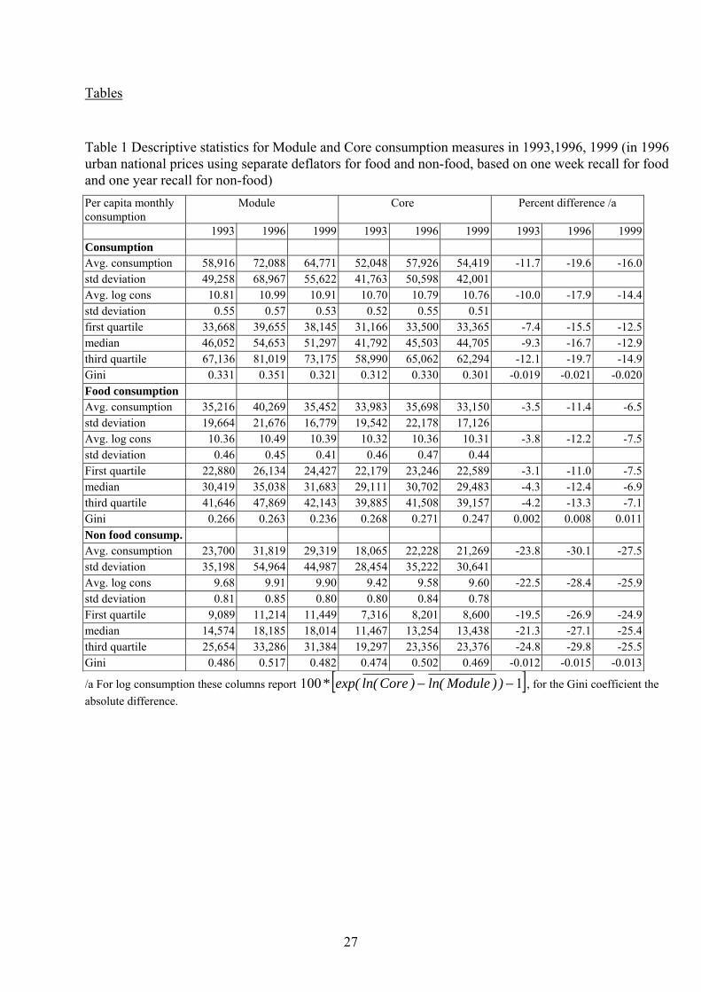
Table 1 shows various summary statistics to describe the distribution of per capita

consumption using the short and long questionnaire for the three years. The differences in the

means turn out higher than what was found during the field test. The degree by which

average consumption is underestimated varies by year, ranging from -11.7 to -19.6 percent.

The degree of underestimation is the highest in 1996, when also average consumption was at

its peak. For food the degree of underestimation of the mean is less, ranging from -3.5

percent in 1993 to -11.4 percent in 1996. The difference in non-food consumption is the

10

largest. The underestimation of the mean ranges from -23.8 percent in 1993 to -30.1 percent

in 1996. The standard deviations for the log per capita consumption are slightly higher for the

Core. Note that when the Core underestimates the Module by a fixed fraction the standard

deviations would have been the same. The higher dispersion stems from the nonfood

consumption, for log food consumption the standard deviations are often smaller for the

Core. The difference between the Core and the Module quartiles increases as the quartile

reflects a wealthier group. This is mostly due to the increasing non-food share in

consumption. Within food and non-food consumption, the differences between the quartiles

is much less pronounced. Inequality, as measured by the Gini coefficient, is slightly higher

for the Core food consumption and Module non-food consumption. Combined, the Module

yields a higher inequality measure total consumption. Although inequality varies

considerably over time, the absolute difference between the Core and the Module Gini

coefficient is quite similar. Figure 1 presents kernel density estimates of log per capita food

and non-food consumption in 1996, the year that the differences are the largest. The shape of

the Core and Module density functions is very similar. In all cases, the Core density function

is slightly more peaked. The dispersion of non-food consumption is much larger than that of

food.

Because we do not have data for the short (from the Core) and the long (from the

Module) consumption measure for the same households, we cannot estimate the function that

maps one into the other directly. A seemingly plausible alternative is to plot the percentiles of

the two consumption measures against each other. If the two questionnaires yield the same

consumption measure, the CDFs should overlap. This is done in Figure 2. The graph is

constructed as follows. Let s denote the log per capita monthly consumption measure

generated by the short questionnaire and l denote the equivalent for the long consumption

11

questionnaire. The function shown in Figure 2 is ( )llGFlls −= − ))((exp/)( 1 where F and G

are the cumulative distribution functions for s and l respectively.

To help interpret the graphs it is instructive to set up a model. Suppose consumption

is distributed log normal and that the long consumption questionnaire measures it with a

multiplicative random lognormally distributed measurement error.

(1) ),(~ 2cnc σµ vcl += ),0(~ 2

vnv σ

where c is the log of consumption. The short consumption questionnaire measures

consumption with systematic bias and random measurement error. Assuming a linear relation

for the systematic bias this yields

(2) εβα ++= cs , ),0(~ 2εσε n

where ε is the random measurement error. Under the above assumptions the CDFs of

l and s can be written as

(3) ⎟⎟

⎠

⎞

⎜⎜

⎝

⎛

+

−=

22)(

vc

xNxGσσ

µ , ⎟⎟

⎠

⎞

⎜⎜

⎝

⎛

+

+−=

222)(

εσσβ

βµα

c

xNxF

where N is the cumulative standard normal distribution function. A mapping of the

distribution functions in this case yields s as a function of l

(4) ( )⎟⎟

⎠

⎞

⎜⎜

⎝

⎛

+

+−++=

22

222

vc

cl)l(sσσ

σσβµβµα ε

It directly follows that when there is no measurement error ( 022 == εσσ v ) the

mapping of the distribution functions yields back the systematic relationship between the two

consumption measures. With measurement error that is not true anymore. Rearranging terms

yields

12

(5) ( )µσσ

βσσ

ββαε

−⎟⎟⎟⎟

⎠

⎞

⎜⎜⎜⎜

⎝

⎛

−+

+++= ll)l(s

vc

c

122

2

22

,indicating that if 22

2

vσβσ ε > ,the function will underestimate the systematic

relationship for values of l below the mean and overestimate for values above the mean. The

above condition holds if the relative measurement error using the short consumption

questionnaire is larger than when using the long consumption questionnaire. Under the same

condition the function’s first derivative with respect to µ is negative. As mean consumption

increases, the last term in (5) will become smaller.

Let’s now turn back to Figure 1. Throughout s(l)/l is smaller than one, indicating that

the short consumption questionnaire systematically underestimates consumption. The

downward sloping section of the curves around the average consumption indicates that as

consumption rises, the fraction by which the short consumption underestimates consumption

increases. In the model above this would imply that 1<β . The upwards sloping section for

low consumption levels and the fading of the downwards sloping trend at high consumption

level also indicates that measurement error is present and that indeed the relative

measurement error for the short consumption is greater than for the long consumption.

Measurement error causes an underestimation at low consumption levels and an

overestimation at consumption levels above the mean. The fact that the curves shift over time

corresponds with the trends in mean consumption. In 1996 average consumption was at its

peak resulting in the lowest estimated s(l)/l function. As demonstrated, this does not

necessarily imply that the systematic relationship between the short and long consumption

measure has changed over time.

13

The presence of measurement error makes it impossible to recover the structural

relationship between the short and long consumption questionnaire by mapping percentiles.

More structure is needed to make progress. Assuming a relationship as postulated in (1), we

can estimate the regression by taking averages over cohorts. Substituting (1) into (2) and

adding an error to take account of model misspecification yields

(6) ijijijijij vls ωβαε +−+=− )(

where j denotes the cohort the household belongs to and i denotes the household. ijω is a

model error term with a conditional mean zero. Taking averages within cohorts yields

(7) jjjjj vls ωβαε +−+=− )()(

Because jε and jv are uncorrelated and tend to zero as the number of observations in the

cohort increases (7) can be estimated by taking averages within each cohort which then serve

as data in the regression. In this analysis, I have used the 298 districts as cohorts. This

approach can be viewed as an application of two sample two stage least squares (Angrist and

Krueger 1992) where the cohort dummies are used as instruments. The identifying

assumption is that the region in which the household lives does not influence short

consumption, conditional on the level of long consumption. In other words, there is no direct

effect of the region in which one lives on the ability to estimate one’s consumption. To allow

for a more flexible functional form I have estimated (8) using locally weighted regression

(lowess). Figure 3 presents the results. On the vertical axis, I have plotted the predicted Core

consumption measure as a ratio of the Module consumption measure, making the figure

directly comparable with Figure 2. Similar curves for food and non-food are presented in

Figure 4.

14

The curves show a similar pattern of systematic underestimation over time. From

1993 to 1999 the systematic underestimation of the Core gradually increased. The vertical

lines in Figure 3 denote the per capita consumption decile cutoff points in 1996. For those in

the poorest two deciles, the Core overestimated Module consumption in 1993. This effect

vanished for the second decile in 1996 and disappeared in 1999. As consumption increases,

the fraction by which the Core underestimates increases also. The curve flattens for the

upper two deciles, suggesting a maximum underestimation of the Core of around 23 percent.

The intertemporal elasticity of the underestimation of the Core is higher than follows

from a purely cross sectional analysis. The line with the three crosses in Figure 3 is

constructed by comparing the mean of log consumption arising from the short and long

questionnaire in the three years. The vertical axis shows by which fraction per capita

consumption is underestimated. Note that this comparison, based on distribution functions, is

valid within the context of the presented model because the last term in (4) vanishes when

µ=l . A one percent increase in average consumption leads to an increase in the

underestimation of the Core of around .45 percent point. Around the mean, the cross sectional

estimates predict an increase in the underestimation of around .2 percent point.

Figure 4 presents the shows the estimates separately for food and non-food

consumption. The elasticity of the underestimation with respect to Module consumption is

higher for food than for non-food. For food, the systematic underestimation increased from

1993 to 1996. From 1996 to 1999, the underestimation increases further for the poor, but

decreases for the rich. This possibly is related to the high food price increases during the

economic crisis. For non-food the pattern is more stable. The maximum underestimation is

around 35 percent.

15

Because the Core and Module questionnaire are nested – every question in the short

consumption questionnaire corresponds to a set of questions in the long consumption

questionnaire – we can make the comparison of averages at a more disaggregated level. Table

2 presents such an analysis for 1996, the year in which the difference was the largest. The

table also shows the effect of using different recall periods for non-food. Official statistics in

Indonesia are based on weekly food consumption and yearly non-food consumption. The

questionnaire however also collects non-food consumption also with a one-month recall

period. Increasing the recall period from one-month to one-year increases the fraction of

underestimation for non-food from –27.8 to –30.1 percent. In food, we find high

underestimations for vegetables, fruits and prepared foods. The difference in prepared food

contributed 15.6 percent to the total difference in consumption. For some food items (tuber,

pulses, spices, alcoholic beverages and tobacco) the average Core consumption turns out

higher than that of the Module. Most of the difference in total consumption, 68 percent, stems

from differences in non-food consumption. Housing clearly is the most problematic non-food

consumption item. The Core underestimates housing by 27 percent contributing about 26

percent to the total difference in consumption. Large differences are also found for

“Miscellaneous goods and services” and durable goods. Although the underestimation for

these items is larger than for housing – around 50 percent – the contribution to the difference

in total consumption is only around 15 percent. The Core overestimates average education

expenditures by around 17 percent.

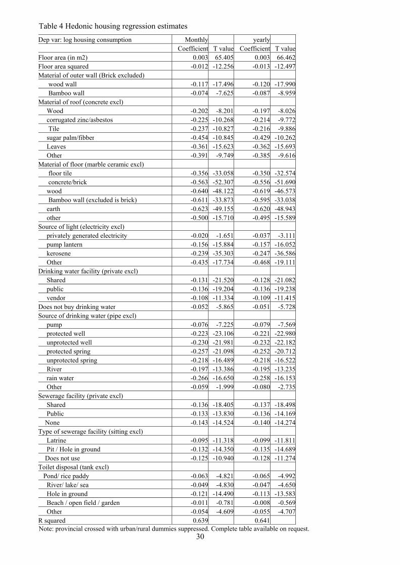
Housing is clearly the most problematic consumption item of all non-food

expenditures. Because of this, I discuss the differences in questionnaire design in more detail

and investigate remedies to solve the discrepancies. The Module housing section asks the

respondents to impute a housing rent if the house is owned or provided free of charge. In

16

addition, the Module consumption questionnaire contains separate questions for maintenance

costs, electricity, water, firewood and several other kinds of fossil fuels or gasses. The Core,

on the other hand, has only one question with no explicit instruction to impute rent for house

owners. One possible remedy to resolve the difference between the Core and Module housing

consumption is to rely on estimates of a hedonic price regression of housing. The Core

contains 11 questions on the quality of the house and sanitary facilities. Since the Core is

administered to all households, we have these data available for both the Core and Module

households. A hedonic price regression based on the Module households, with log housing

expenditures as the dependent variable and the housing quality variables along with a set of

regional dummies as independent variables yields and R squared of .64. The estimated

coefficients are in Table 4.

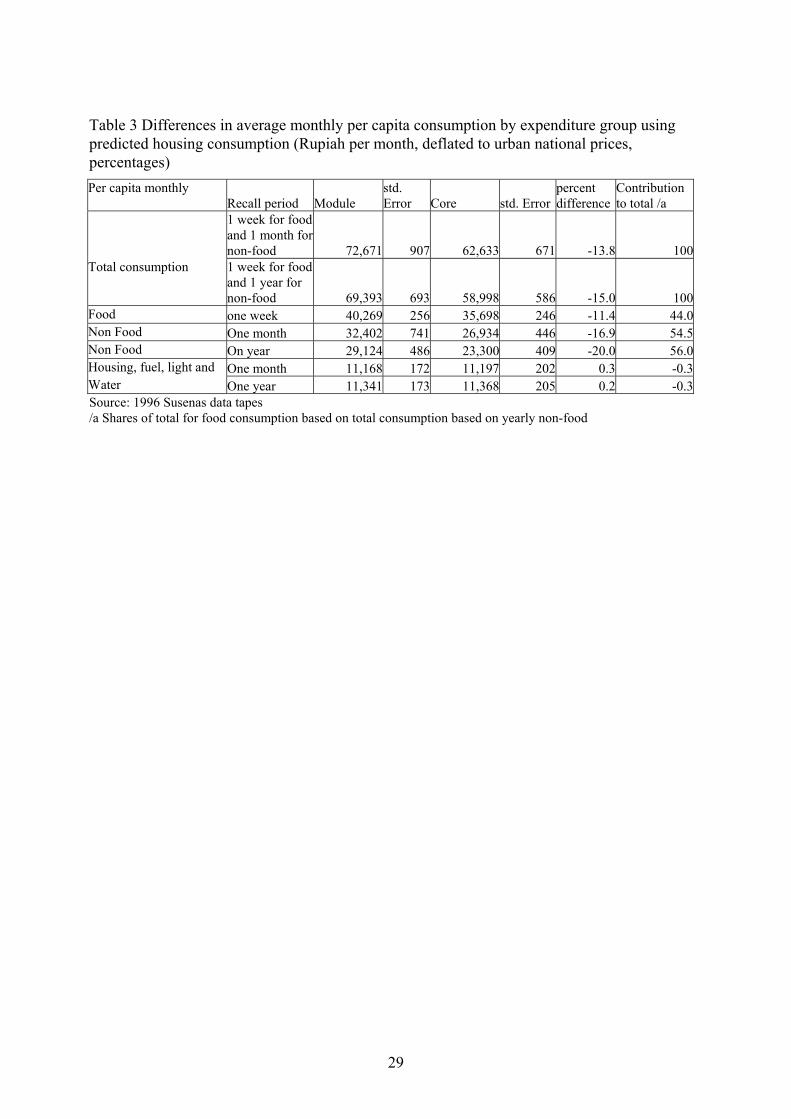
As expected, there is no significant difference between the Core and Module

households when using predicted housing consumption4 (see Table 3 , as a result of the

random assignment of questionnaires). The mean predicted consumption however is

substantially smaller than the mean actual consumption from the Module households. To the

extent that this is caused by measurement error (resulting from the difficulty the respondent

has in estimating an imputed rent), it may be desirable to use the predicted housing

consumption instead of the actually reported. Using predicted housing consumption reduces

the difference in total consumption between the Core and Module to 14 to 15 percent,

depending on the reference period used for non-food consumption.

In the remainder of the paper, I will use a consumption measure were housing is not

imputed. Although I believe the consumption measure with imputed housing consumption is

4 I use the smearing estimate as proposed by Duan (1983) which is defined as ∑−∗ )ˆexp(N)ˆxexp( ii εβ 1

17

preferable, an important objective of the paper is to investigate the usefulness of the Core

consumption measure given that the official statistics are based only on the actual Module

consumption.

4. Welfare analysis

Now we turn to the question of what one can do in terms of welfare analysis when

one only has the short consumption questionnaire available. This is a question of practical

importance in Indonesia. In two out of every three years, the Susenas only collects

consumption data using the short consumption questionnaire. The question is also of general

importance for researchers basing their analysis on consumption data generated from short

questionnaires who wish to have a handle on the magnitude of the errors they are making.

We will discuss the consequences of using the short consumption questionnaire for

three types of analysis commonly found in the poverty literature. The first is poverty

measurement. How well can we measure poverty by constructing an adjusted poverty line for

the Core? The second type is “rank” analysis. In this type of analysis, the population is

ranked according to a welfare measure, usually per capita consumption. Next, income

inequality of a non-consumption welfare measure, such as enrollment or malnutrition, is

investigated. Concentration curves or quintile tables are common examples. The crucial

distinction here is that the analysis is based only on the rank that an individual holds in the

per capita consumption distribution. The third type is “gradient” analysis. Here we are

interested in the elasticity of a non-consumption welfare measure with respect to per capita

consumption. This type of analysis typically involves estimating a regression with the non-

18

consumption welfare measure as the dependent variable and log per capita consumption as

one of the explanatory variables.

Measurement error complicates the analysis of poverty. Measurement error increases

the poverty estimate as long as the poverty line is below the mode of the consumption

distribution. Measurement error increases the probability weight of tails of the distribution,

which is the basis of the poverty estimate. For the head count ratio, the effects are easily

demonstrated using the model as postulated in (1) and (2). Let z denote the log poverty line.

The head count ratio based on the long consumption measure is )(zG which overestimates

poverty if there is measurement error ( 0>vσ ) and z<µ. Using zzs βα += as a poverty line

for the short consumption measure5 yields as a head count ratio )z(F s which also

overestimates poverty if 0>εσ and βµα +<sz . The latter estimate will yield a higher

poverty estimate than the one based on the long consumption measure if the relative

measurement error of the short consumption measure exceeds that of the long one

)/( 222vσβσ ε > .

One seemingly plausible way around this problem is to adjust the poverty line for the

Core such that it yields the same head count for a given year: ))z(G(Fzs1−= . This can be

done for a year that both the Module and Core are available. For the other years the head

count ratio can be analyzed using the short consumption measure in conjunction with the

newly established “short poverty line”. Such an approach however is not valid. Working

through the same derivation as above, it immediately follows from (5) that the short poverty

5 Lanjouw and Lanjouw (1999) study the effect of using a partial consumption measure (food consumption) for

poverty measurement. Their approach is similar in that they use the estimated Engel curve whereas I l use

19

line depends on µ , the average consumption. An updating rule that would ensure the same

head count ratio under the assumption of constant variances of the log consumption and

measurement error is

(8) ( )stst

vc

c

stst zz ,,122

2

22

,,1 1 µµσσ

βσσ ε

−⎟⎟⎟⎟

⎠

⎞

⎜⎜⎜⎜

⎝

⎛

−+

+−= ++

where s,tz is the anchored short poverty line for a year that both the Core and the

Module are available and βµαµ +=s , the mean of the log Core consumption measure.

Table 5 presents head count ratios6. The poverty line is set at 38,246 Rupiah per

capita in urban 1996 prices and applied to the Module data. Two sets of poverty lines are

applied to the Core. The first is constructed by applying for each year separately the

structural relationship as depicted in Figure 3. For the second set of poverty lines is

constructed such that it yields the same head count ratio as the Module data. As expected the

Core poverty estimates based on the first set exceed those of the Module. The relative

measurement error of the Core is higher than that of the Module. The differences are

substantial; the head count ratio is around 4 percent point higher if the Core data are used.

The second set gives us an idea of how the poverty line needs to be updated as average

consumption rises. In (6), we can take first differences of the log poverty lines and the mean

log Module consumption figures (from Table 1). This yields an estimate of 0.947 (1993-

1996) and 0.976 (1996-1999) for the large expression in brackets in (8). The expression can

the estimated structural relation between the short and the long consumption measure estimated in the previous section.

6 The estimates differ from those reported earlier in for instance Pradhan, Suryahadi, Sumarto and Pritchett (2000) or Biro Pusat Statistik (1996). The reason for this is that I use in this study price deflators which reflect general consumption patterns whereas most poverty studies use the regional poverty lines as price

20

be used as an estimate of minus the elasticity of the Core poverty line with respect to mean

log Core consumption if one’s objective is to obtain the same head count ratio as when the

Module were used. It does not imply equality of the higher order FGT poverty measures.

Even though the estimate is rather constant over time, it is larger that we expected. In terms

of the model, it would imply an extremely large relative measurement error in the Core.

There is clearly room for improvement. The linear model for the systematic part of the model

(which does not show from Figure 3) and normality pose overly strong restrictions on the

model. If the objective is to predict Module poverty based on Core data, these will need to be

relaxed. This is however beyond the scope of this paper. All I demonstrated is that both

measurement error and systematic underestimation have to be accounted for when embarking

on such an endeavor.

In the rank analysis, my prior is that the concentration curves based on the short

consumption to show less income inequality than the one based on the Module consumption.

If the structural underestimation is a monotonically increasing function of Module

consumption (as found in Figure 3), it will not change the ranking. The measurement error

causes a reclassification, resulting in a weaker relation between consumption and benefits.

Since the underestimation is higher for the rich, the effect of the measurement error will be

less for the higher income groups.

Since the Core collects a range of non-consumption welfare measures for both the

Core and Module households identically, I can test my expectations empirically. As non-

welfare measures I use school enrolment for children in the junior and senior secondary age

deflators. In the latter the food share is higher. Readers interested in absolute levels of poverty should refer to the studies quoted above.

21

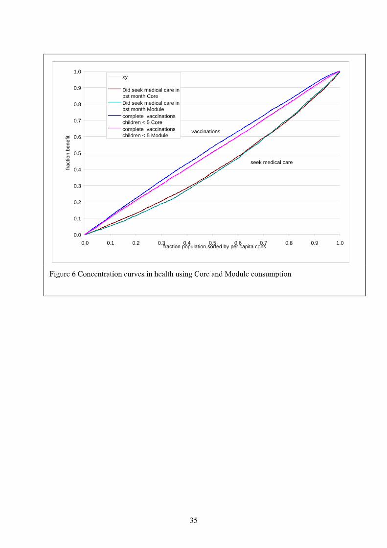
group, whether the respondent sought medical care in the past month and whether young

children received a complete set of vaccinations. Figure 5 and Figure 6 present the

concentration curves generated separately using the Core and Module consumption measure.

In general, the concentration curves lie remarkably close. For all but the curve for

vaccinations, we find that the expected relation that the using the short consumption shows

less income inequality for the lower income groups. Only for the vaccination we find that the

Core yield a slight pro-poor bias while the Module indicates no income dependence.

In the gradient analysis, my prior is that the estimated elasticities based on the Core

are higher than those based on the Module. Suppose we wish to obtain the consumption

elasticity of some non-consumption welfare measure y. In that case the elasticity can be

estimated by

(9) ηγδ ++= ly

where the variable of interest is γ . Because of omitted variables on the RHS of the equation,

consumption needs to be instrumented. Let Z be a vector of instruments for consumption

(10) ωϕ += Zc

Equations (1), (9) and (10) can be estimated by two stage least squares. The resulting

estimate of γ is an unbiased estimate of the elasticity of consumption. Instrumenting

eliminates the bias caused by measurement error in l. When l is replaced by s in equation (9),

and s is a function of c as postulated in (2), instrumenting s with Z will yield an estimate of

the elasticity divided by β . Because the short consumption measure rises more slowly than

the long as true consumption rises, the estimate of γ will be an overestimate. By estimating

both models separately for the Core and the Module we can investigate the magnitude of this

bias.

22

For the gradient problem, I present estimates of γ in (9) using the housing variables

collected in the Core as instruments (see Table 4 for a full list). For the Core column I

replaced l by s and used the same instruments. The results are in Table 6. As expected, the

estimate of γ is higher if the short consumption measure is used. The ratio of the two

estimates of γ varies from .60 to .92. One possible explanation for the large differences is that

the equations have been estimated for different subsamples (enrolment only for children,

contact rate for all) and that the linear approximation assumed in (2) varies by group. Based

on the large differences it does not seem realistic to suggest correction for gradient estimates

based on the Core.

5. Conclusions

This paper exploited a repeated large-scale experiment in Indonesia allowing an

examination of the effect of using fewer questions to collect consumption data. The analysis

indicates that using fewer questions yields a lower consumption measure. The fraction by

which consumption is underestimated increases as consumption rises. Whether or not a short

consumption questionnaire suffices, thus depends on the level of economic development,

which is directly related to the variety of consumption patterns and the share of non-food in

total consumption. For the case of Indonesia, reducing the number of questions from around

320 to 23 yields to a underestimation of consumption ranging from 12 to 20 percent over the

period from 1993 to 1999. Imputing rent values using a hedonic price approach decreases the

underestimation by 6 percent point in 1996.

23

Away from the mean, a comparison based on mapping percentiles is not valid in the

presence of measurement error. I estimated the structural underestimation of the Core

consumption measure by applying two sample two stage least squares using regional cohorts

as instruments. The curvature of the relationship is similar over time although the degree of

underestimation still rises with average consumption. In 1999, the cross sectional elasticity

flattened for food consumption probably as a result of the high increases in food prices and

the less varied diet that followed.

The effects of using a shorter consumption measure for welfare analysis vary. Even

after purging the systematic underestimation of short consumption measure, measurement

error still causes higher poverty estimates if the short consumption measure is used. I

suggested a method to update the poverty lines for the Core if one’s objective is to equalize

the head count ratios. Concentration curves, which are based on the rank in the individual

holds in the consumption distribution, are very similar for both consumption measures. The

point estimates in a gradient analysis are higher when the Core is used and the ratio by which

the Core overestimates the consumption elasticity varies substantially depending on which

welfare measure is used. It thus seems unadvisable to rely on the short consumption measure

for gradient analysis.

The design of the Susenas survey seems to strike a good balance between cost

effectiveness and precision, which may be applied elsewhere. As the effect of using less

questions increases as consumption rises, the model seems more suitable for low income

countries. Collecting consumption using few questions allows for welfare analysis, especially

where the main interest is in ordering households from poor to rich. Correction factors can be

developed using those years in which the long questionnaire is administered along with the

24

short questionnaire. Regular anchoring of these factors appears necessary as the structural

relationships vary over time.

25

References:

Angrist, Joshua and Alan Krueger (1992) “The Effect of Age at School Entry on Education

Attainment: An Application of Instrumental Variables with Moments from Two

Samples”, Journal of the American Statistical Association, vol 87, no418, pp328-336.

Asra, Abuzar (1999) “Urban-Rural Differences in Costs of Living and Their Impact on

Poverty Measures”, Bulletin of Indonesian Economic Studies; v35 n3 December

1999, pp. 51-69.

Biro Pusat Statistik (1996, 1999) “Statistical Yearbook”, Central Bureau of Statistics, Jakarta,

Indonesia.

Deaton, Angus and Salman Zaidi (1999) “Guidelines for Constructing Consumption

Aggregates for Welfare Analysis”, working paper, Princeton University.

Duan, Naihua (1983) “Smearing Estimate: A Nonparametric Retransformation Method”,

Journal of the American Statistical Association, vol 78, nr 383, pp 605-610.

Elbers, Chris, Jean O. Lanjouw and Peter Lanjouw (2000) “Welfare in villages and Towns”

Tinbergen Institute Discussion paper no 029/2, Amsterdam.

International Monetary Fund (2000) “International Financial Statistics” , Washington DC

Joliffe, Dean and Kinnon Scott (1995) “The sensitivity of measures of household

consumption to survey design: results from an experiment in El Salvador, Policy

research Department, World Bank, Washington DC.

Lanjouw, Jean Olsen and Peter Lanjouw (1999) “Can we Compare Apples and Oranges?

Poverty Measurement based on Different Definitions of Consumption”, working

paper, Yale University.

Montgomery, Mark R., et al. (2000) “Measuring Living Standards with Proxy Variables”,

Demography v37, n2 (May 2000): 155-74.

26

Pradhan, Menno, Asep Suryahadi, Sudarno Sumarto and Lant Pritchett (2000)

“Measurements of Poverty in Indonesia: 1996, 1999, and Beyond”, SMERU working

paper, Jakarta, Indonesia.

Sahn, David and David Stifel (2000) “Exploring Alternative Measures of Welfare in the

Absence of Expenditure Data”, draft mimeo, Cornell University.

Shubham Chaudhuri, Martin Ravallion (1994), How well do static indicators identify the

chronically poor?, Journal Of Public Economics (53)3 (1994) pp. 367-394

Statistical Institute and Planning Institute of Jamaica (1996) Jamaica survey of living

conditions, 1994 Kingston, Jamaica.

Surbakti, Pajung (1997) “Indonesia’s National Socio-Economic Survey: a continual data

source for analysis on welfare development”, Central Bureau of Statistics, Jakarta,

Indonesia.

Tummers (1994) “The effect of Systematic Misperception of Income on the Subjective

Poverty Line”, in The Measurement of Household welfare, eds Blundell, Preston and

Walker, Cambridge University Press.

World Bank (1992) “Indonesia: Public Expenditures, prices and the poor”, Indonesia

Resident mission 11293-IND, Jakarta.

World Bank (1999,2000) “World Development Report”, World Bank, Washington DC.

27

Tables

Table 1 Descriptive statistics for Module and Core consumption measures in 1993,1996, 1999 (in 1996 urban national prices using separate deflators for food and non-food, based on one week recall for food and one year recall for non-food) Per capita monthly consumption

Module Core Percent difference /a

1993 1996 1999 1993 1996 1999 1993 1996 1999Consumption Avg. consumption 58,916 72,088 64,771 52,048 57,926 54,419 -11.7 -19.6 -16.0std deviation 49,258 68,967 55,622 41,763 50,598 42,001 Avg. log cons 10.81 10.99 10.91 10.70 10.79 10.76 -10.0 -17.9 -14.4std deviation 0.55 0.57 0.53 0.52 0.55 0.51 first quartile 33,668 39,655 38,145 31,166 33,500 33,365 -7.4 -15.5 -12.5median 46,052 54,653 51,297 41,792 45,503 44,705 -9.3 -16.7 -12.9third quartile 67,136 81,019 73,175 58,990 65,062 62,294 -12.1 -19.7 -14.9Gini 0.331 0.351 0.321 0.312 0.330 0.301 -0.019 -0.021 -0.020Food consumption Avg. consumption 35,216 40,269 35,452 33,983 35,698 33,150 -3.5 -11.4 -6.5std deviation 19,664 21,676 16,779 19,542 22,178 17,126 Avg. log cons 10.36 10.49 10.39 10.32 10.36 10.31 -3.8 -12.2 -7.5std deviation 0.46 0.45 0.41 0.46 0.47 0.44 First quartile 22,880 26,134 24,427 22,179 23,246 22,589 -3.1 -11.0 -7.5median 30,419 35,038 31,683 29,111 30,702 29,483 -4.3 -12.4 -6.9third quartile 41,646 47,869 42,143 39,885 41,508 39,157 -4.2 -13.3 -7.1Gini 0.266 0.263 0.236 0.268 0.271 0.247 0.002 0.008 0.011Non food consump. Avg. consumption 23,700 31,819 29,319 18,065 22,228 21,269 -23.8 -30.1 -27.5std deviation 35,198 54,964 44,987 28,454 35,222 30,641 Avg. log cons 9.68 9.91 9.90 9.42 9.58 9.60 -22.5 -28.4 -25.9std deviation 0.81 0.85 0.80 0.80 0.84 0.78 First quartile 9,089 11,214 11,449 7,316 8,201 8,600 -19.5 -26.9 -24.9median 14,574 18,185 18,014 11,467 13,254 13,438 -21.3 -27.1 -25.4third quartile 25,654 33,286 31,384 19,297 23,356 23,376 -24.8 -29.8 -25.5Gini 0.486 0.517 0.482 0.474 0.502 0.469 -0.012 -0.015 -0.013

/a For log consumption these columns report [ ]1100 −− ))Moduleln()Coreln(exp(* , for the Gini coefficient the absolute difference.

28

Table 2 Differences in average monthly per capita consumption by expenditure group (Rupiah per month, deflated to urban national prices, percentages)

Per capita monthly Recall period Module std. Error Core std. Error percent difference

Contribution to total /a

1 week for food and 1 month for non-food 75,722 1,057 61,279 648 -19.1 100.0

Total consumption (based on yearly non food)

1 week for food and 1 year for non-food 72,088 863 57,926 623 -19.6 100.0

Food one week 40,269 256 35,698 246 -11.4 32.3Non Food One month 35,453 889 25,580 477 -27.8 68.4Non Food On year 31,819 666 22,228 438 -30.1 67.7Cereals one week 9,442 39 9,107 57 -3.5 2.4Tuber one week 497 11 652 11 31.2 -1.1Fish one week 3,468 43 3,165 40 -8.7 2.1Meat one week 2,315 44 1,972 46 -14.8 2.4Egg and Milk one week 2,121 29 1,937 29 -8.7 1.3Vegetables one week 3,623 30 2,546 29 -29.7 7.6Pulses one week 1,420 15 1,498 15 5.5 -0.6Fruit one week 2,075 31 1,495 31 -27.9 4.1Oil and Fat one week 1,765 12 1,709 16 -3.2 0.4Beverage flavor one week 2,196 16 2,102 18 -4.3 0.7Spice one week 1,028 9 1,175 11 14.3 -1.0Miscellaneous food one week 920 15 830 14 -9.7 0.6prepared food one week 6,106 93 3,895 119 -36.2 15.6alcoholic beverages one week 57 4 104 11 83.3 -0.3tobacco and betel one week 3,236 29 3,510 42 8.5 -1.9Housing, fuel, light and One month 14,219 381 9,843 241 -30.8 30.9Water One year 13,803 360 10,062 229 -27.1 25.9Miscellaneous goods One month 5,224 156 2,448 72 -53.1 19.6And services One year 4,722 142 2,142 66 -54.6 17.9Education costs One month 1,930 56 2,470 127 28.0 -3.8 One year 2,089 56 2,434 144 16.5 -2.4Health costs One month 2,463 95 2,520 122 2.3 -0.4 One year 1,227 38 1,126 34 -8.2 0.7Clothing foodwear One month 4,034 89 3,134 71 -22.3 6.4Headgear One year 3,812 49 2,499 37 -34.5 9.1durable goods One month 5,350 511 2,909 143 -45.6 17.2 One year 3,718 124 2,027 85 -45.5 11.7taxes and insurance One month 834 28 790 43 -5.3 0.3 One year 1,033 50 781 27 -24.4 1.7festivities and One month 1,398 135 1,465 85 4.8 -0.5Ceremonies One year 1,415 46 1,156 41 -18.3 1.8 Source: 1996 Susenas data tapes /a Shares of total for food consumption based on total consumption based on yearly non-food

29

Table 3 Differences in average monthly per capita consumption by expenditure group using predicted housing consumption (Rupiah per month, deflated to urban national prices, percentages) Per capita monthly

Recall period Module std. Error Core std. Error

percent difference

Contribution to total /a

1 week for food and 1 month for non-food 72,671 907 62,633 671 -13.8 100

Total consumption 1 week for food and 1 year for non-food 69,393 693 58,998 586 -15.0 100

Food one week 40,269 256 35,698 246 -11.4 44.0Non Food One month 32,402 741 26,934 446 -16.9 54.5Non Food On year 29,124 486 23,300 409 -20.0 56.0Housing, fuel, light and One month 11,168 172 11,197 202 0.3 -0.3Water One year 11,341 173 11,368 205 0.2 -0.3Source: 1996 Susenas data tapes /a Shares of total for food consumption based on total consumption based on yearly non-food

30

Table 4 Hedonic housing regression estimates Dep var: log housing consumption Monthly yearly

Coefficient T value Coefficient T valueFloor area (in m2) 0.003 65.405 0.003 66.462Floor area squared -0.012 -12.256 -0.013 -12.497Material of outer wall (Brick excluded) wood wall -0.117 -17.496 -0.120 -17.990 Bamboo wall -0.074 -7.625 -0.087 -8.959

Material of roof (concrete excl) Wood -0.202 -8.201 -0.197 -8.026 corrugated zinc/asbestos -0.225 -10.268 -0.214 -9.772 Tile -0.237 -10.827 -0.216 -9.886 sugar palm/fibber -0.454 -10.845 -0.429 -10.262 Leaves -0.361 -15.623 -0.362 -15.693 Other -0.391 -9.749 -0.385 -9.616

Material of floor (marble ceramic excl) floor tile -0.356 -33.058 -0.350 -32.574 concrete/brick -0.563 -52.307 -0.556 -51.690 wood -0.640 -48.122 -0.619 -46.573 Bamboo wall (excluded is brick) -0.611 -33.873 -0.595 -33.038 earth -0.623 -49.155 -0.620 -48.943 other -0.500 -15.710 -0.495 -15.589

Source of light (electricity excl) privately generated electricity -0.020 -1.651 -0.037 -3.111 pump lantern -0.156 -15.884 -0.157 -16.052 kerosene -0.239 -35.303 -0.247 -36.586 Other -0.435 -17.734 -0.468 -19.111

Drinking water facility (private excl) Shared -0.131 -21.520 -0.128 -21.082 public -0.136 -19.204 -0.136 -19.238 vendor -0.108 -11.334 -0.109 -11.415

Does not buy drinking water -0.052 -5.865 -0.051 -5.728Source of drinking water (pipe excl) pump -0.076 -7.225 -0.079 -7.569 protected well -0.223 -23.106 -0.221 -22.980 unprotected well -0.230 -21.981 -0.232 -22.182 protected spring -0.257 -21.098 -0.252 -20.712 unprotected spring -0.218 -16.489 -0.218 -16.522 River -0.197 -13.386 -0.195 -13.235 rain water -0.266 -16.650 -0.258 -16.153 Other -0.059 -1.999 -0.080 -2.735

Sewerage facility (private excl) Shared -0.136 -18.405 -0.137 -18.498 Public -0.133 -13.830 -0.136 -14.169 None -0.143 -14.524 -0.140 -14.274

Type of sewerage facility (sitting excl) Latrine -0.095 -11.318 -0.099 -11.811 Pit / Hole in ground -0.132 -14.350 -0.135 -14.689 Does not use -0.125 -10.940 -0.128 -11.274

Toilet disposal (tank excl) Pond/ rice paddy -0.063 -4.821 -0.065 -4.992 River/ lake/ sea -0.049 -4.830 -0.047 -4.650 Hole in ground -0.121 -14.490 -0.113 -13.583 Beach / open field / garden -0.011 -0.781 -0.008 -0.569 Other -0.054 -4.609 -0.055 -4.707

R squared 0.639 0.641 Note: provincial crossed with urban/rural dummies suppressed. Complete table available on request.

31

Table 5 Poverty estimates with Core and Module data (percentages) 1993 1996 1999

Module poverty line 38,246 38,246 38,246 head count ratio 35.0 22.4 25.2Core poverty line 36,981 35,207 34,671Poverty line adjusted using structural relationship

Head count ratio 39.4 28.9 28.0

Core poverty line 35,187 32,378 33,454Poverty line adjusted so that the head count ratios are the same

Head count ratio 35.0 22.4 25.2

Table 6 Estimate of elasticity of per capita consumption using long and short consumption measure

Module Core coeff std error Coeff std error

primary school enrollment

0.390 0.0140 0.446 0.0172

junior secondary 0.543 0.0200 0.667 0.0238contact rate 0.0149 0.0023 0.0245 0.0037

Full set of shots 0.255 0.0172 0.275 0.0206Note: Housing variables collected in Core used as instruments

32

Figures:

0.0

0.1

0.2

0.3

0.4

0.5

0.6

0.7

0.8

0.9

1.0

7 8 9 10 11 12 13

log per capita consumption

prob

abiit

y de

nsity

CoreModule

non-food

food

total

Figure 1 Kernel density estimates for per capita monthly consumption in 1996

33

0.7

0.75

0.8

0.85

0.9

0.95

9.5 10 10.5 11 11.5 12

log per capita module consumption

Cor

e/M

odul

e199319961999

Figure 2 Mapping of distribution functions of per capita consumption of Core and Module (1996 national urban prices)

0.6

0.7

0.8

0.9

1

1.1

1.2

1.3

10 10.2 10.4 10.6 10.8 11 11.2 11.4 11.6 11.8 12

log per capita Module consumption

Cor

e/M

odul

e

199319961999means

Figure 3 Systematic underestimation of Core consumption (vertical lines denote thresholds for 1996 Module consumption deciles)

34

0.6

0.7

0.8

0.9

1

1.1

1.2

1.3

8.5 9 9.5 10 10.5 11 11.5

log per capita module consumption

Cor

e/M

odul

e

199319961999

non-food

food

Figure 4 Systematic underestimation of Core food and non-food consumption

0.0

0.1

0.2

0.3

0.4

0.5

0.6

0.7

0.8

0.9

1.0

0.0 0.1 0.2 0.3 0.4 0.5 0.6 0.7 0.8 0.9 1.0

cumulative fraction population sorted by per capita consumption

cum

ulat

ive

shar

e en

rollm

ent

xy

enrolment children 13-15 Core

enrolment children 13-15 Module

enrolment children 16-18 Core

enrolment children 16-18 Module

16-18

13-15

Figure 5 Concentration curves for education using Core and Module consumption

35

0.0

0.1

0.2

0.3

0.4

0.5

0.6

0.7

0.8

0.9

1.0

0.0 0.1 0.2 0.3 0.4 0.5 0.6 0.7 0.8 0.9 1.0fraction population sorted by per capita cons

fract

ion

bene

fit

xy

Did seek medical care inpst month CoreDid seek medical care inpst month Modulecomplete vaccinationschildren < 5 Corecomplete vaccinationschildren < 5 Module

seek medical care

vaccinations

Figure 6 Concentration curves in health using Core and Module consumption