Embed Size (px)
Citation preview

Graduate Theses, Dissertations, and Problem Reports
2021
Weed Recognition in Agriculture: A Mask R-CNN Approach Weed Recognition in Agriculture: A Mask R-CNN Approach
Sruthi Keerthi Valicharla West Virginia University, [email protected]
Follow this and additional works at: https://researchrepository.wvu.edu/etd
Part of the Other Electrical and Computer Engineering Commons
Recommended Citation Recommended Citation Valicharla, Sruthi Keerthi, "Weed Recognition in Agriculture: A Mask R-CNN Approach" (2021). Graduate Theses, Dissertations, and Problem Reports. 8102. https://researchrepository.wvu.edu/etd/8102
This Thesis is protected by copyright and/or related rights. It has been brought to you by the The Research Repository @ WVU with permission from the rights-holder(s). You are free to use this Thesis in any way that is permitted by the copyright and related rights legislation that applies to your use. For other uses you must obtain permission from the rights-holder(s) directly, unless additional rights are indicated by a Creative Commons license in the record and/ or on the work itself. This Thesis has been accepted for inclusion in WVU Graduate Theses, Dissertations, and Problem Reports collection by an authorized administrator of The Research Repository @ WVU. For more information, please contact [email protected].

Graduate Theses, Dissertations, and Problem Reports
2021
Weed Recognition in Agriculture: A Mask R-CNN Approach Weed Recognition in Agriculture: A Mask R-CNN Approach
Sruthi Keerthi Valicharla
Follow this and additional works at: https://researchrepository.wvu.edu/etd
Part of the Other Electrical and Computer Engineering Commons

Weed Recognition in Agriculture: A Mask R-CNN Approach
Sruthi Keerthi Valicharla
Thesis submitted to the Benjamin M. Statler College of Engineering and Mineral Resources
at West Virginia University in partial fulfillment of the
requirements for the degree of
Master of Science in
Electrical Engineering
Xin Li, Ph.D., Chair Roy S. Nutter, Ph.D.
Katerina Goseva- Popstojanova, Ph.D.
Lane Department of Computer Science and Electrical Engineering
Morgantown, West Virginia 2021
Keywords: Mask R-CNN, Mile-A-Minute, Localized Style Transfer, UAVs, Data Augmentation, Detectron2
Copyright 2021 Sruthi Keerthi Valicharla

Abstract
Weed Recognition in Agriculture: A Mask R-CNN Approach
Sruthi Keerthi Valicharla
Recent interdisciplinary collaboration on deep learning has led to a growing interest in its
application in the agriculture domain. Weed control and management are some of the crucial tasks
in agriculture to maintain high crop productivity. The inception phase of weed control and
management is to successfully recognize the weed plants, followed by providing a suitable
management plan. Due to the complexities in agriculture images, such as similar colour and
texture, we need to incorporate a deep neural network that uses pixel-wise grouping for identifying
the plant species. In this thesis, we analysed the performance of one of the most popular deep
neural networks aimed to solve the instance segmentation (pixel-wise analysis) problems: Mask
R-CNN, for weed plant recognition (detection and classification) using field images and aerial
images. We have used Mask R-CNN to recognize the crop plants and weed plants using the
Crop/Weed Field Image Dataset (CWFID) for the field image study. However, the CWFID's
limitations are that it identifies all weed plants as a single class and all of the crop plants are from
a single organic carrot field. We have created a synthetic dataset with 80 weed plant species to
tackle this problem and tested it with Mask R-CNN to expand our study.
Throughout this thesis, we predominantly focused on detecting one specific invasive weed type
called Persicaria Perfoliata or Mile-A-Minute (MAM) for our aerial image study. In general,
supervised model outcomes are slow to aerial images, primarily due to large image size and
scarcity of well-annotated datasets, making it relatively harder to recognize the species from higher
altitudes. We propose a three-level (leaves, trees, forest) hierarchy to recognize the species using
Unmanned Aerial Vehicles(UAVs) to address this issue. To create a dataset that resembles weed
clusters similar to MAM, we have used a localized style transfer technique to transfer the style
from the available MAM images to a portion of the aerial images' content using VGG-19
architecture. We have also generated another dataset at a relatively low altitude and tested it with
Mask R-CNN and reached ~92% AP50 using these low-altitude resized images.
iii
Acknowledgements
First and foremost, I would like to express my deep appreciation and indebtedness to my committee
chair and research advisor, Dr. Xin Li, for his endless support and invaluable advice throughout
my MS journey. His expertise in various domains provided me an opportunity to work with the
agriculture department. I would also like to extend my gratitude to Dr. Yong-Lak Park for his
constant feedback and resources. Without their knowledgeable advice and timely suggestions, this
thesis would not have been possible.
I would also like to thank my committee members Dr. Roy S. Nutter and Dr. Katerina Goseva-
Popstojanova, for their support, time, and encouragement. I’m forever grateful to Dr. Brian M.
Powell for providing me an opportunity to work as a GTA for CS 101.
I’m much obliged to my late grandma Vijayalakshmi Velavarthipati for her constant motivation to
pursue my higher education. I’m thankful to my cousin Sandhya Mynampati for her continuous
love and support. Immense thanks to my friend Anusha Kandula for all the countless favours
throughout my life in the States. Special thanks to Dr. Satish GVS.
Finally, I owe my gratitude to my parents Dr. Anuradha Devi Velavarthipati, Sreenivasa Rao V.V,
and my brother Surya Praneeth V. for their unconditional love and encouragement.

iv
Table of Contents
Abstract…………………………………………………………………………………………..ii
Acknowledgments……………………………………………………………….………………iii
List of Figures…………………………………………………………………………………..vii
List of Tables……………………………………………………………………………………..x
Chapter 1: ...................................................................................................................................... 1
Introduction: ................................................................................................................................. 1
1.1 Motivation:.......................................................................................................................................... 1
1.1.1 Classification vs. Localization vs. Detection: ................................................................................ 2
1.1.2 Object detection: ......................................................................................................................... 2
1.1.3 Image Segmentation: ................................................................................................................... 3
1.1.4 Data Augmentation: ..................................................................................................................... 4
1.1.5: Weeds in Agriculture: ................................................................................................................. 4
1.2 Deep Learning for weed recognition: ................................................................................................. 7
1.3 Problem Statement: ............................................................................................................................ 8
1.3.1 Ground level weed plants recognition using Mask R-CNN: ......................................................... 8
1.3.2 Synthetic Dataset creation using Neural Style Transfer and Geometrical transformations: ...... 9
1.3.3 MAM detection using Mask R-CNN: ............................................................................................ 9
1.4 Contribution: ....................................................................................................................................... 9
1.5 Dissertation Structure: ...................................................................................................................... 10
Chapter 2: .................................................................................................................................... 11
Literature Survey: ...................................................................................................................... 11
2.1 Related Work: ................................................................................................................................... 11
2.2 Neural Style Transfer: ....................................................................................................................... 13
2.2.1 Introduction: .............................................................................................................................. 13
2.2.2 Style transfer vs. localized style transfer: .................................................................................. 16
2.2.3 NST for Agriculture dataset: ....................................................................................................... 16
2.3 Detectron2: ....................................................................................................................................... 16
2.3.1 Introduction: .............................................................................................................................. 16
2.3.2 Data Loader, Models, and Data Augmentation: ........................................................................ 18

v
2.3.3 Training and Evaluation of models: ........................................................................................... 19
Chapter 3: .................................................................................................................................... 21
Weed recognition using Mask R-CNN:..................................................................................... 21
3.1: Introduction to Mask RCNN: ............................................................................................................ 21
3.2: Network architecture: ...................................................................................................................... 33
3.3: Feature extraction with Feature Pyramid Network: ........................................................................ 34
3.4: Dataset: ............................................................................................................................................ 36
3.4.1: CWFID dataset with mask: ........................................................................................................ 36
3.4.2: Synthetic COCO dataset: ........................................................................................................... 38
3.5: Average Precision:............................................................................................................................ 41
3.6: Experiment setup: ............................................................................................................................ 42
3.6.1 Using CWFID: .............................................................................................................................. 42
3.6.2 Using Synthetic COCO dataset: .................................................................................................. 43
3.7: Results and Discussion: .................................................................................................................... 43
Chapter 4: .................................................................................................................................... 46
Data Augmentation for Aerial Images: ..................................................................................... 46
4.1 Introduction: ..................................................................................................................................... 46
4.2 Style Transfer: ................................................................................................................................... 47
4.2.1 Introduction: .............................................................................................................................. 47
4.2.2 Localized Style Transfer: ............................................................................................................ 47
4.2.3 VGG19 network Architecture: .................................................................................................... 48
4.2.4 VGG19 for style transfer: ........................................................................................................... 50
4.2.5 Hyperparameters: ...................................................................................................................... 54
4.2.6 Dataset: ...................................................................................................................................... 55
4.2.7 Experiment setup: ...................................................................................................................... 56
4.2.8 Results and Discussion: .............................................................................................................. 57
4.3 MAM Dataset with Geometrical Transformations: .......................................................................... 60
4.3.1 Procedure: .................................................................................................................................. 60
4.3.2 Mask Generation:....................................................................................................................... 63
4.3.3 Annotations: ............................................................................................................................... 65
4.3.4 Limitations: ................................................................................................................................ 65
Chapter 5: .................................................................................................................................... 66
MAM Detection using Mask R-CNN: ....................................................................................... 66
vi
5.1 Introduction: ..................................................................................................................................... 66
5.2 Three – Level Hierarchy for MAM detection: ................................................................................... 70
5.3 Experiment Setup:............................................................................................................................. 72
5.4 Results and Evaluations: ................................................................................................................... 72
5.5 Ablation study: .................................................................................................................................. 74
Chapter 6: .................................................................................................................................... 76
Conclusions and Future Work: ................................................................................................. 76
6.1 Conclusions: ...................................................................................................................................... 76
6.2 Future Work: ..................................................................................................................................... 76
Bibliography ................................................................................................................................ 79

vii
List of Figures
Figure 1.1: Figure illustrating the difference between classification, localization, detection, and
instance segmentation. .................................................................................................................... 2
Figure 1.2: Difference between semantic segmentation (left) and instance segmentation (right).
Source ............................................................................................................................................. 3
Figure 1.3: Drones in agriculture. Source ....................................................................................... 5
Figure 1.4: Drones for irrigation and crop spraying. Source. ......................................................... 6
Figure 1.5: Drones for 3D mapping. Source ................................................................................... 7
Figure 2.1: An example of Neural Style Transfer. (a) Content image, (b) Style image, (c)
Generated image. Source .............................................................................................................. 14
Figure 2.2: Convolutional Neural Networks for NST. The input image is passed through various
filters and the number of filters increase as we proceed to the deeper layers. The size of the
image will be decreasing due to down-sampling. ......................................................................... 15
Figure 3.1: Working of CNN. ....................................................................................................... 22
Figure 3.2: Selective search algorithm for object localization. Source ........................................ 24
Figure 3.3: Object detection using R-CNN................................................................................... 26
Figure 3.4: Intersection over Union. (a) Red bounding box is ground truth and the blue bounding
box is the predicted bounding box. (b) Intersection of the bounding boxes. (c) Union of the
bounding boxes. ............................................................................................................................ 27
Figure 3.5: The network architecture of R-CNN. ......................................................................... 28
Figure 3.6: The network architecture of Fast R-CNN. ................................................................. 29
Figure 3.7: The network architecture of Faster R-CNN. .............................................................. 30
Figure 3.8: Working of RPN. Source [33] .................................................................................... 31
Figure 3.9: The network architecture of Mask R-CNN. ............................................................... 33
Figure 3.10: Pyramid architecture. (a) Pyramid of images. (b) Pyramid of feature maps. Source
[42] ................................................................................................................................................ 34
Figure 3.11: Dataflow in an FPN. Source [42] ............................................................................. 34
Figure 3.12: Working principle of ResNet. Source [43] ............................................................... 36

viii
Figure 3.13: Images from CWFID. (a) RGB image of weed and crop plants. (b) Annotated image
with the red colour being the weed plant and green colour being the carrot crop plant. Source [5]
....................................................................................................................................................... 37
Figure 3.14: Example images from the COCO type CWFID dataset. .......................................... 38
Figure 3.15: Types of images used for creating the synthetic data with 80 classes. (a) Foreground
examples. (b) Background examples. ........................................................................................... 39
Figure 3.16: Example image from the COCO type Synthetic dataset. ......................................... 40
Figure 3.17: IoU = 0.5 (left), IoU= 0.75 (right) ............................................................................ 42
Figure 3.18: COCO type CWFID’s Mask R-CNN results with Softmax threshold = 0.9. The
number on the top of the bounding box is the probability of the plant being a specific class like
Crop_Plant or Weed_Plant. .......................................................................................................... 43
Figure 3.19: Synthetic COCO dataset’s Mask R-CNN results with Softmax threshold = 0.5. The
number on the top of the bounding box is the probability of the plant being a specific class like
Class_1 – Class_80. ...................................................................................................................... 44
Figure 4.1: The network architecture of VGG19. ......................................................................... 48
Figure 4.2: Concept of NST with CNN. ....................................................................................... 51
Figure 4.3: Computation of Style Matrix with 5 feature maps in a CNN layer. Source ............... 52
Figure 4.4: An example of localized style transfer. (a) content image, (b) Mask of the content
image, (c) Generated image with a random style. Source [6] ....................................................... 54
Figure 4.5: Sample images of Agriculture-Vision dataset’s weed cluster class. (a) RGB image of
the weed cluster, (b) Binary mask for the RoI. Source [6] ........................................................... 55
Figure 4.6: Real-time MAM aerial images with manually marked MAM regions. ..................... 56
Figure 4.7: Content, Mask and Style images used for our data augmentation using NST. .......... 57
Figure 4.8: Procedure for mask augmentation using Albumentations. ......................................... 60
Figure 4.9: RGB (left) and binary mask (right) of the MAM aerial image. ................................. 61
Figure 4.10: Block diagram for binary mask generation for the marked aerial RGB images. ..... 64
Figure 4.11: Output of each block. (1) RGB image, (2a) Red channel of the RGB image, (2b)
Grayscale of the RGB image, (3) Difference of 2a and 2b, (4) Difference image after denoising,
(5) Binary image of the difference image, (6) Final mask after morphological reconstruction. .. 64
Figure 4.12: Example images from the Augmented MAM dataset. ............................................. 65

ix
Figure 5.1: MAM infestation in the US (left) and areas in the east coast infected by MAM
(right). Source ............................................................................................................................... 67
Figure 5.2: Leaves (left) and fruits (right) of MAM. Source ........................................................ 68
Figure 5.3: Spraying of herbicides for the entire field. Source ..................................................... 69
Figure 5.4: Hand plucking weeds. Source .................................................................................... 69
Figure 5.5: MAM weevil for biological control. Source .............................................................. 70
Figure 5.6: Flow chart for our three-level hierarchy..................................................................... 71
Figure 5.7: Augmented dataset’s (section 4.3) Mask R-CNN results with Softmax threshold =
0.9. The number on the top of the bounding box is the probability of MAM’s presence. ........... 72
Figure 5.8: Augmented dataset’s (section 4.3) Mask R-CNN results with Softmax threshold =
0.5. With this threshold, we have false alarms such as car detection. .......................................... 73
Figure 5.9: Mask R-CNN’s performance on real-time data. ........................................................ 75
Figure 6.1: Three-level hierarchy. (1) Forest level, (2) Trees level, (3) Plant level. .................... 77
Figure 6.2: MAM in various lighting conditions. ......................................................................... 77
Figure 6.3: Weeds similar to MAM: Japanese Stilt grass (left) and Hedge Bindweed (right) ..... 78

x
List of Tables
Table 1: Statistical comparison between other datasets and our synthetic dataset ....................... 40
Table 2: Comparison of Mask R-CNN’s performance on ground-level plant recognition image
with CWFID.................................................................................................................................. 44
Table 3: ConvNet configuration of VGG19 ........................................................................... 49-50
Table 4: Illustration of Global style transfer with and without colour transfer from the style
image to the content image. .......................................................................................................... 53
Table 5: Results of our NST data augmentation with VGG19 ................................................ 58-59
Table 6: Geometrical transformations on the RGB images and masks of aerial MAM data using
Albumentations. ....................................................................................................................... 62-63
Table 7: COCO evaluation metrics for different RPN backbones. ............................................... 74
Sruthi Keerthi Valicharla 1
Chapter 1:
Introduction:
Agriculture is one of the ancient and vital professions in the world. Over the millennia,
humanity embraced various technologies like AI to boost productivity and efficiency in
agriculture, thereby reduce negative environmental impacts. One of the greatest threats that the
farmers face is low crop yields to weed infestations. Weed plants reduce the crop yield by ~50%
[1], which can have severe economic effects. Some of the most widely used methods to eliminate
weed plants are using herbicides or robots powered with AI. The former option is inexpensive, but
there is a chance that these herbicides might contaminate the crop plants, thereby posing a health
risk. However, the latter option is a bit expensive, but it does not require human labour, and it will
not cause any health risks. Hence, the usage of AI in agriculture has been prevalent nowadays.
1.1 Motivation:
Deep learning is a part of Machine Learning that mimics the human brain's workings in
processing the data for object detection, recognition, and decision making. A convolutional neural
network (CNN) [2] is a subclass of deep neural networks, generally applied to analyse visual
images. CNNs are inspired by biological processes in which the connectivity pattern between
neurons resembles the animal visual cortex's organization. CNNs use relatively fewer image pre-
processing blocks compared to other image classification algorithms. Due to its promising results
in visual recognition tasks, deep learning has been deployed into the agriculture sector.

Sruthi Keerthi Valicharla 2
1.1.1 Classification vs. Localization vs. Detection:
One of the many enduring questions in the field of Computer Vision is, "What are the
differences between Classification, Localization, and Detection?" Image classification is a
relatively easy task compared to localization and detection. Image classification involves assigning
a particular label to an image that gives us the details about that image's class. Object Localization
involves creating a bounding box around the objects within an image, but it does not specify
anything about the image's class. However, detection, on the other hand, involves creating a
bounding box around the region of interest (RoI) and assigning a class to the different objects in
the image. Hence, object detection is a combination of Image classification and localization. Often,
the whole procedure for object detection is referred to as Object recognition. The figure below
illustrates the difference between classification, localization, and detection.
Figure 1.1: Figure illustrating the difference between classification, localization, detection, and instance segmentation.
1.1.2 Object detection:
Object detection is a vital computer vision task that deals with detecting objects of a particular
class such as birds, people, vehicles in digital images and videos. Other applications of object
detection include face detection, facial recognition, tracking objects, and video surveillance.
Therefore, to gain a complete understanding of an image, instead of restricting our concentration
to classifying images, we should expand it to precisely estimate objects' locations in a digital
image. In this task, the input will be an image containing one or more distinguishable objects, and
the output will be an image containing bounding boxes around those distinguishable objects and a
Chapter 1: Introduction

Sruthi Keerthi Valicharla 3
label indicating the class of that object in the bounding box. The object recognition task can be
further improved by adding Image Segmentation.
1.1.3 Image Segmentation:
Image segmentation involves drawing the bounding boxes around the objects in the input image
at a pixel level. By doing so, we can differentiate many identical objects within a single input
image. Image segmentation helps us analyse the image by breaking down the input image into
segments containing the pixels of objects and pixels of the background. This pixel-wise
segmentation will give us the object's shape instead of just creating a rectangular bounding box
around the object. Image segmentation can be classified into two levels of granularity: Semantic
segmentation and Instance segmentation.
• Semantic Segmentation: This is a process of detecting all the objects in an image and
grouping them based on their categories. For example, all human beings are categorized
into one category and all vehicles into another category.
• Instance Segmentation: This process is an advancement over semantic segmentation as it
involves detecting the individual objects within the defined categories. For instance, it
distinguishes each human-like adult, kid, and vehicle into cars, bikes.
The figure below provides us a better understanding of the difference between Semantic and
Instance segmentation.
Figure 1.2: Difference between semantic segmentation (left) and instance segmentation (right). Source1
1 https://www.analyticsvidhya.com/blog/2019/04/introduction-image-segmentation-techniques-python/.
Chapter 1: Introduction

Sruthi Keerthi Valicharla 4
1.1.4 Data Augmentation:
At times in deep learning tasks, lack of a sufficient dataset will create hindrances. One of the
most straightforward solutions for this problem is to create a synthetic dataset. However, the
synthetic images generated must be identical to the real-time images to get promising results. To
do so, we used the Neural Style Transfer technique (NST) [3] and geometrical transformations.
NST takes two images as input - a content image and a style reference image - and blends them so
that the output image retains the core elements of the content image and acquires the style/texture
of the style reference image. While the geometrical transformations, on the other hand, uses
transformations on an image to obtain more images.
1.1.5: Weeds in Agriculture:
As per the Weed Science Society of America, a weed is defined as a plant whose growth is
undesirable in a field, leading to ecological imbalances and economic loss. Occasionally, these
weeds might also lead to health problems in human beings and animals. Some of the examples of
weed plants are Poison Ivy, Tree of heaven. Taxonomically speaking, there is no actual
significance for the word 'weed.' It is always subjective because a plant can be a weed in one
context but not in another. Sometimes beneficial weeds are intentionally grown in the gardens.
Often, weeds can grow invasively or aggressively outside the species' natural habitat. As per the
natural enemies’ hypothesis2, certain plants become very dominant when introduced into new
ambiences due to a lack of fauna that feeds on them or lack fauna that competes with them.
Some of the drawbacks of having weeds in horticulture are:
• They compete with the crop plants for food, water, sunlight, and soil nutrients.
• They cause skin irritations to homo-sapiens and may cause discomfort in the animals'
digestive tracts as some of the weeds contain thorns, burs, and even toxins.
• They can act as a host for several pathogens that might degrade the crop production,
2 Positive correlation between plants and their natural enemies.
Chapter 1: Introduction

Sruthi Keerthi Valicharla 5
• Weeds might damage other engineering works such as water sprinklers, drains,
foundations.
• They cause degradation of lawns' aesthetic appearance, golf courses, and botanical gardens
with their unappealing appearance.
It is essential to remove the weeds from the agricultural fields to prevent all the drawbacks
mentioned above. The most prevalent methods to remove the weeds are using herbicides, lethal
wilting, using mulch3. However, if the field area is vast, it is slightly harder to monitor the crop
plants with limited human labour. Also, we need an expert to identify the species, and there aren't
very many technicians that can do this job. So, this led to the usage of drones/UAVs to improve
crop efficiency. Drone technology is an exceptional innovation with its uses in multiple domains.
These drones can help the farmers to monitor crop spraying, irrigation mapping. UAVs aid in
achieving so-called precision agriculture. In short, precision agriculture can be referred to as 'using
fewer resources to grow more.' One of the limitations of using drones is that they are pricey.
Nevertheless, as the population is increasing, the need for farming will only increase. The demand
for drones in the agriculture market will increase in the future, leading to a decline in the price.
Farmers face many challenges that influence the success of their crops. Some of the challenges
include climate change, soil quality, weeds, insect infestation. Farmers are tending towards UAVs
to provide faster, reliable, and efficient results to address these issues.
Figure 1.3: Drones in agriculture. Source4
3 material (such as decaying leaves, bark, or compost) spread around or over a plant to enrich or insulate the soil. 4 https://www.greenbiz.com/article/making-drones-work-small-farmers.
Chapter 1: Introduction

Sruthi Keerthi Valicharla 6
Uses of drones in agriculture:
Drones are usually equipped with IR cameras, GPS, programmable controllers, navigation units
to collect data related to weeds, soil quality, and nutrients. This data can be used to get more precise
information about the issues. Let us look at how drones answer some of the common issues in
agriculture.
1. Crop Spraying: To maintain high crop yields, farmers need to spray herbicides, fertilizers,
and pesticides. Conventional ways of spraying include using an automobile, aeroplanes, or
even manual. Usage of these traditional methods is time-consuming and expensive.
However, drones can solve this problem very quickly. The only additional requirement is
they need to be equipped with reservoirs that can be filled with pesticides. This method is
also helpful when we have to spray pesticides only to certain plants in the field instead of
the whole field. This type of spraying is often referred to as spot spraying.
2. Irrigation Management: Like the previous functionality, drones can monitor crop plants
to spot irrigation problems. Using drones, we can avoid water pooling or identify areas
with less than the required moisture content. To do so, the drones must be equipped with
thermal cameras.
Figure 1.4: Drones for irrigation and crop spraying. Source5
5 https://www.thomasnet.com/insights/drone-use-in-agriculture-is-soaring-to-new-heights/.
Chapter 1: Introduction

Sruthi Keerthi Valicharla 7
3. Seed Planting: Drones are not yet widely used to solve this problem, but experiments are
still going on for the effective use of drones to shoot seeds into ploughed soil.
4. Soil Analysis: Soil analysis includes identifying nutrient requirements, soil quality
analysis, and identification of dead/barren lands. The drones must be equipped with
instruments that can capture the 3D maps to obtain the soil information.
Figure 1.5: Drones for 3D mapping. Source6.
5. Crop Surveying: This is by far the essential application of using drones in the field of
agriculture. Traditionally, plane images and satellite images are used to get farm images.
Nevertheless, obtaining information from satellites can be outdated. With NIR drones,
plant health can be easily determined by calculating the amount of light absorbed.
As deep learning models do an excellent job identifying most common objects like cars, people,
our objective is to use the very idea to detect the plant species using drone images.
In this thesis, our primary focus is one weed called Persicaria Perfoliata or Mile-A-Minute
(MAM).7
1.2 Deep Learning for weed recognition:
Deep learning mimics the human brain's workings for processing the data using multiple
network layers to extract higher-level features from the raw input images and hence used for many
6 https://pilotinstitute.com/drone-mapping/. 7 http://nyis.info/invasive_species/mile-a-minute/.
Chapter 1: Introduction

Sruthi Keerthi Valicharla 8
visual recognition tasks. In the field of agriculture, all the objects (plants and weeds) will be mostly
green in colour (green on green), so object recognition (in our case, species identification) is
relatively more complicated as most of the object recognition algorithms use colour, fill, texture
and size for object recognition (refer to section 3.1). To eliminate the false positives problem, we
propose a three-level hierarchy (refer to section 5.1) for identifying weeds using UAV images. The
hierarchy is as follows:
1. Forest level (very high-altitude images)
2. Tree level (low-altitude images)
3. Leaf level (ground-level images)
1.3 Problem Statement:
In this thesis, we report our ground level and low altitude image studies. Our key focus is on
the following problems.
1. Leaf level: Weed plant species recognition using Mask R-CNN.
2. Tree level: Synthetic Dataset creation using Neural Style Transfer and geometrical
transformations.
3. Mask R-CNN's performance analysis with the augmented data produced in statement 2.
1.3.1 Ground level weed plants recognition using Mask R-CNN:
In this study, we used Mask R-CNN [4] to distinguish the weed plants among the crop plants.
To achieve this task, we used the Crop/Weed Field Image Dataset (CWFID) [5]. However, this
dataset's limitation is that it classifies all the weed plants into a single class and the crop plants are
of single species. To expand our study, we used 80 foreground images of weed plants to create a
synthetic dataset. We labelled them as class 1 through class 80.
Chapter 1: Introduction
Sruthi Keerthi Valicharla 9
1.3.2 Synthetic Dataset creation using Neural Style Transfer and Geometrical
transformations:
In this part of our study, we primarily focused on a particular invasive weed plant called Mile-
A-Minute (MAM). We aim to detect MAM plants using Unmanned Aerial Vehicles (UAVs). As
we are using a supervised model for our MAM predictions, the number of data points is
proportional to the number of trainable parameters of a model, which is proportional to the
complexity of the task that needs to be achieved. Hence, we need to have an adequately annotated
dataset to use Mask R-CNN or any other supervised learning network. Since we could get only a
few real-time UAV images of MAM, we used Neural Style Transfer (NST) technique to create our
synthetic dataset. For the content images, we used the Agriculture Vision dataset [6], and for the
style reference, we used our UAV images. We used VGG 19 [7] architecture to accomplish our
NST task. Due to this dataset’s limitations, we have created one more synthetic dataset using
geometrical transformations. We have used transformations such as flips, rotations, and grid
distortions to achieve the data augmentation task in the latter dataset.
1.3.3 MAM detection using Mask R-CNN:
In this section, we focused on detecting MAM regions using UAV images. Being an aggressive
invasive plant, MAM can decrease the crop plant’s ability to photosynthesize8 and potentially kill
the plants by smothering them with their weight (refer to section 5.1). So, detection of MAM zones
is vital for the crop fields with MAM infestation. Using the low-altitude images mentioned in
section 1.3.2, we trained Mask R-CNN to recognize the MAM zones and reached an AP50 ~97%
for bounding box and AP50~ 92% segmentation.
1.4 Contribution:
• We created a synthetic dataset with 80 foreground images, thereby classifying them into
80 classes, and fed the dataset to Mask R-CNN.
8 The process of synthesizing food from sunlight, CO2 and H2O
Chapter 1: Introduction

Sruthi Keerthi Valicharla 10
• We have created synthetic datasets using a localized style transfer technique and
geometrical transformations technique.
• We tested Mask R-CNN's performance on the real-time augmented data.
1.5 Dissertation Structure:
The remainder part of this thesis is organized as follows:
• Chapter 2 focuses on the literature review about detectron2 and style transfer.
• Chapter 3 reviews the experimental setup and dataset details used for ground-level weed
recognition using Mask R-CNN.
• Chapter 4 focuses on various data augmentation techniques for aerial images, including
NST and geometrical transformations
• Chapter 5 presents our approach to detect MAM using Mask R-CNN.
• Chapter 6 focuses on conclusions and future work.
Chapter 1: Introduction

Sruthi Keerthi Valicharla 11
Chapter 2:
Literature Survey:
2.1 Related Work:
In the recent past, many deep learning models were introduced for object recognition tasks.
However, when it comes to the agriculture domain, the object recognition task is challenging as
the weed plants and crop plants might have the same colour, texture, fill, and size. Classification
is a relatively easy task compared to the recognition tasks at lower altitudes, to be precise on a leaf
level. There are many public datasets at the leaf level for species identification [8], disease
prediction in one [9], or more species [10] [11]. However, when it comes to real-time applications,
we need to focus on datasets at the plant level. There have been many advances in these plant-
level classification tasks. Most agriculture datasets focus on diseased crop identification. Very few
datasets like DeepWeeds [12] focus on weed plants that grow among the crop plants. However,
DeepWeeds focus on eight different species that are native to northern Australia, and it does not
provide any data about the localization of the plants, thereby restricting it to classification tasks.
The lighting of the image also plays a crucial role in agriculture tasks along with the quality. Most
of the mentioned datasets have a single lighting condition. Carrot-Weed [13] is a dataset that
provides images at different lighting conditions, but as the name suggests, the crop images are
restricted to carrot plants. Specific datasets like Plant Phenotyping [14], Plant Seedling dataset
[15], and others [16] provide us information about the vegetation areas, but the limitation of these

Sruthi Keerthi Valicharla 12
datasets is that the background is soil or stones instead of other plants. Even at the plant level,
without proper annotations indicating specific plant species' location, it is hard to recognize the
species among several plants. Recent advances in the field of object detection lead to the
collaboration of agriculture and deep learning fields to achieve precision agriculture [17] [18].
Usage of CNNs for detecting weeds among certain plants like turfgrass [19], ryegrass [20],
soybeans [21] was proven to be a suitable method for weed management. Along with the
supervised models, unsupervised models with minimal labelling have also been in use for the weed
detection [22]. In this thesis, we have created a synthetic dataset of 80 weed species with more
than one class per image to expand our study on Mask R-CNNs performance on weed recognition.
For our aerial image study, we focused on recognizing MAM using UAV images. Due to the
ever increase in population, the demand for growing food is expected to increase despite limited
farmlands. To grow more food with fewer resources, farmers are now adapting the so-called
Precision Agriculture. Precision agriculture involves modern technology usage, including but not
restricted to drones and dusters for crop management. Although drones are not currently allowed
for every agricultural need (such as carrying harmful substances) due to Federal Aviation
Administration (FAA) regulations, dusters9 can still be used for crop management as they fly at
very low altitude (10 foot above the ground). However, dusters are far more expensive than drones.
However, drones can be used for crop management following the FAA regulations. Recognizing
the agriculture patterns such as weed recognition can be very challenging at a very high altitude.
Using the multispectral images taken by drones, we can detect the plant species. There are very
few datasets [6] [23] created for pattern recognition in agriculture. Hence, we propose a three-level
hierarchy (forests, trees, and leaves) for confirming the presence of MAM in a given field, with
the forest being the high altitude, trees being the low-altitude, and leaves being the ground-level
images. In this thesis, we analysed the performance of Mask R-CNN at low altitude and ground
levels. As there are no specific datasets dedicated to MAM recognition, we created synthetic data
using NST and standard augmentation techniques.
9 Usage of aerial vehicles for dusting the crops
Chapter 2: Literature Survey

Sruthi Keerthi Valicharla 13
2.2 Neural Style Transfer:
2.2.1 Introduction:
Neural Style Transfer (NST) is an illustration of image stylization within the field of Non-
Photorealistic Rendering (NPR). NPR is a subset of Computer Graphics (CG) focusing on enabling
a wide range of expressive styles for digital art. Unlike conventional CG, NPR does not focus on
photorealism10. Due to its inspiration from other artistic modes such as animations, drawing,
painting, NPR is often used in movies and video games. The first two illustration-based style
transfer algorithms were based on patch-based texture synthesis algorithms called image analogies
[24] and Image Quilting [25].
Texture synthesis is generally used to fill in holes in images like inpainting11 or expand the
small pictures. Texture synthesis algorithmically constructs a large image from a small digital
sample. There are multiple techniques to achieve this goal. Some of the techniques available are
patch-based texture synthesis, pixel-based texture synthesis, tilting, stochastic texture synthesis.
Early style transfer algorithms are based on patch-based texture synthesis. Patch-based Texture
synthesis is faster and effective compared to pixel-based texture synthesis because the patch-based
texture synthesis creates a new texture by replicating and stitching other textures at various offsets.
Image analogies, Image quilting, and graph-cut textures are some of the best patch-based texture
synthesis algorithms.
• Image Analogies: It is a process of creating an image filter from training data. Texture
mapping is used for texture synthesis from an example texture image. For a given image
pair containing an image and an artwork of that image, by analogy, a transformation can
be learned to create new artwork from another image.
• Image Quilting: A new image is synthesized by stitching small patches of existing images.
It can be used only for a single style.
10 a style of art characterized by the highly detailed depiction of ordinary life with the impersonality of a
photograph. 11 Inpainting is a conservation process where damaged, deteriorating, or missing parts of an artwork are filled in
to present a complete image. [Wikipedia]
Chapter 2: Literature Survey

Sruthi Keerthi Valicharla 14
Image Quilting was later used for Texture transfer by rendering an object with a texture that is
taken from another object [25].
Nowadays, deep learning and neural network approaches are proven to be fast and powerful.
The publication of the article "A Neural Algorithm of Artistic Style" in 2015 [3] laid the foundation
for the usage of Convolutional Neural Networks (CNNs) to the problem of style transfer in image
processing. Style transfer is a procedure that involves transferring the style of one image to another
while preserving the content of the target image. The figure below is an illustration of NST.
(a) (b) (c)
Figure 2.1: An example of Neural Style Transfer. (a) Content image, (b) Style image, (c) Generated image. Source12
CNNs usually consist of multiple layers of computational units. Each computational unit layer
can be defined as a collection of image filters that can extract the desired features from the image
that is fed as an input. The output of each layer will be a divergent representation of the filtered
input images called feature maps. When we train a CNN for an object recognition problem, the
feature maps usually care about the image's actual content compared to its pixel values. In
general, the lower layers capture the low-level information such as precise pixel values, whereas
the higher layers, on the other hand, capture the high-level information such as the arrangement of
an object in the image, which is the content itself. Often, the higher layers are referred to as content
representation. With this idea as a baseline, NST is developed. While performing the style transfer,
instead of training a neural network, we start with a blank image and cost function and alter each
pixel iteratively to reduce the cost function. In short, instead of updating biases and weights while
12 https://www.wikiart.org/en/wassily-kandinsky.
Chapter 2: Literature Survey
Sruthi Keerthi Valicharla 15
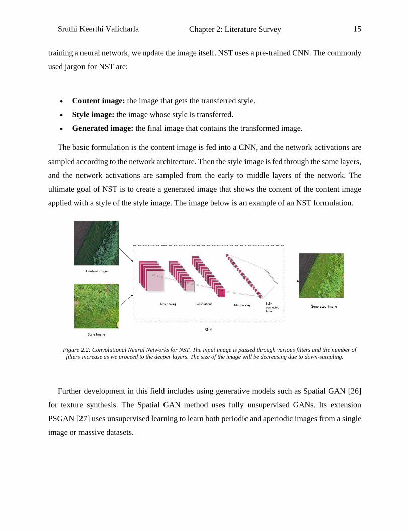
training a neural network, we update the image itself. NST uses a pre-trained CNN. The commonly
used jargon for NST are:
• Content image: the image that gets the transferred style.
• Style image: the image whose style is transferred.
• Generated image: the final image that contains the transformed image.
The basic formulation is the content image is fed into a CNN, and the network activations are
sampled according to the network architecture. Then the style image is fed through the same layers,
and the network activations are sampled from the early to middle layers of the network. The
ultimate goal of NST is to create a generated image that shows the content of the content image
applied with a style of the style image. The image below is an example of an NST formulation.
Figure 2.2: Convolutional Neural Networks for NST. The input image is passed through various filters and the number of
filters increase as we proceed to the deeper layers. The size of the image will be decreasing due to down-sampling.
Further development in this field includes using generative models such as Spatial GAN [26]
for texture synthesis. The Spatial GAN method uses fully unsupervised GANs. Its extension
PSGAN [27] uses unsupervised learning to learn both periodic and aperiodic images from a single
image or massive datasets.
Chapter 2: Literature Survey

Sruthi Keerthi Valicharla 16
2.2.2 Style transfer vs. localized style transfer:
Majority of the style transfer applications require the transfer of the style to the entire image.
Nevertheless, at times we need a partial-image style transfer called localized style transfer13 [28]
[29]. In this dissertation, we have used a localized style transfer technique to create a synthetic
dataset. This localized style transfer involves selecting specific regions in the input image that
needs a style transfer (usually by using masks) and then applying the style transfer to that masked
region, thereby leaving the unmasked region unaltered.
2.2.3 NST for Agriculture dataset:
Lack of a properly annotated dataset can affect the overall performance of the object detection
models. This problem is more challenging for agriculture tasks such as weed recognition and crop
recognition due to a lack of public datasets. Compared to standard data augmentations techniques
like flipping and rotating, NST has proven to provide better accuracy when it comes to
classification tasks [30]. We can create a synthetic dataset that resembles the original crop images
to address our lack of proper annotated dataset problem by using NST. In this thesis, we have
generated a synthetic dataset using some aerial images as content images and MAM images as
style images.
2.3 Detectron2:
2.3.1 Introduction:
Object recognition is one of the fundamental visual recognition tasks in the field of Computer
Vision. Over the past few years, numerous implementations of object recognition algorithms have
been made on various open-source platforms. Deep learning architectures like Convolutional
Neural Networks (CNNs) can automatically learn object features by analysing thousands of
13 https://github.com/cysmith/neural-style-tf.
Chapter 2: Literature Survey
Sruthi Keerthi Valicharla 17
training images to identify various objects in an image. Traditionally, there are two approaches to
recognize objects using deep learning.
• Training a model from scratch: In this approach, we need numerous labelled training
images. We also must set up layers and weights to design a model that can accurately learn
the training data features and provide precise predictions on the testing data.
• Transfer learning: In this approach, we use a procedure called fine-tuning. This approach
is less time-consuming and is widely used in Deep Learning applications because we feed
a new dataset with unknown classes to an existing model such as VGG 16 [7], MobileNet
[31], that has already been trained on several thousands of images.
Detectron is an open-source software that implements most state-of-the-art algorithms for
Object detection and classification. It is implemented using Caffe214, a deep learning framework.
Detectron has become one of the most used open-source platforms by Facebook AI Research
(FAIR)15. However, as Detectron is built on the Caffe2 framework, its purpose has been restricted
to production use. Caffe2 primarily focuses on scalable systems and cross-platform support for
applications that involve large-scale object detection and classification. For the research flexibility
and applicability, PyTorch is a preferred choice.
PyTorch vs. Caffe2:
Caffe2 is more developer friendly than PyTorch when it comes to model deployments on
various platforms like Android, Raspberry Pi, iOS. Caffe2 has the upper hand in deploying the
models over PyTorch because Caffe2 can run on any platform once coded. Also, most of the
networks written in PyTorch can be deployed in Caffe2.
However, when it comes to flexibility issues involved in research, such as parameter alterations,
model changes, and debugging, PyTorch has the upper hand. Due to PyTorch's dynamic nature, it
14 https://developer.nvidia.com/blog/caffe2-deep-learning-framework-facebook. 15 https://ai.facebook.com/.
Chapter 2: Literature Survey

Sruthi Keerthi Valicharla 18
can overcome TensorFlow's limitations and Keras16 as well. Hence, for the research applications,
PyTorch will be a better option.
Facebook's research team developed Detrectron217, a second generation of the Detectron library
using the PyTorch framework to support research and production applications. Detectron2 is very
flexible and provides fast training on single or multiple GPU servers. Detectron218 is a modular
design that allows us to plug custom module implementations into any part of an object detection
system.
2.3.2 Data Loader, Models, and Data Augmentation:
Data Loaders are the components that take raw information from the provided datasets and
process them into a format that the model requires. Detectron2 has a built-in data loader, but it also
allows the user to define their own data loader (custom data loader). Throughout this thesis, we
used the existing data loader provided by Detectron2. To understand the data loader's working, we
need to understand the functionality of build_detection_{train, test}_loader, the two functions
provided by Detectron2 to create a data loader from a chosen config. It loads a list containing a
registered dataset's lightweight format such as PASCAL VOC, COCO [32] and performs a few
pre-processing tasks like augmentation and memory allocation. Each dictionary in this list is
mapped by using a function called mapper. This mapper function transforms the dataset's
lightweight representation into a model-ready representation by applying augmentation, allocating
memory, and performing torch tensor conversions. This output is batched and fed to a model.
Data Augmentation19 is a procedure used to increase data images' number by using slightly
altered copies of existing data. Detectron2's data augmentation allows us to augment multiple data
types such as images with masks and images with bounding boxes together. It also facilitates the
users to add custom new data types such as rotated bounding boxes and manipulate the operations
16 https://keras.io/. 17 https://github.com/facebookresearch/detectron2. 18 https://detectron2.readthedocs.io/en/latest/. 19 https://en.wikipedia.org/wiki/Data_augmentation.
Chapter 2: Literature Survey
Sruthi Keerthi Valicharla 19
applied by augmentations. We can also use a sequence of geometrical augmentations. For more
advanced applications, we can customize the transform strategy by performing a geometrical
inversion of the transform, new data type addition such as coordinates, masks, polygons, and much
more.
Detectron2 includes the following object detection models: Faster R-CNN [33], Mask R-CNN
[4], RetinaNet [34], Cascade R-CNN [35], and Panoptic FPN [36], and many more to come.
Detectron2 uses GPU for the entire training pipeline, thereby making it faster than Detectron. Each
dict (dictionary) obtained from the data loader corresponds to a single image. The Key points
required are model-dependent. Based on our requirements, we can use the model for training or
inference. If we use the model in training mode, all the training statistics are stored. However, if
we want to perform inference with an existing model, we have to use DefaultPredictor wrapper to
perform pre-processing, model loading, and batch operations. The model's input is a list of
dictionaries containing the keys like image channel information, desired output's height and width,
instances such as masks and key-points, bounding box information. The output will be a dictionary
that includes all the losses.
2.3.3 Training and Evaluation of models:
One of the most useful features of Detectron2 is that it allows the users to customize their
training loop. Once the model and data loader are ready, we can write our training loop by using
the tool provided by PyTorch, thereby giving the users full control over the training logic.
However, we can also use the standard trainer abstraction that simplifies the training process as
well. DefaultTrainer is the most often used trainer abstraction compared to SimpleTrainer20. The
DefaultTrainer allows the users to perform all the default configurations for the optimizer, learning
rates, checkpoints, evaluations, and logging. Whereas the SimpleTrainer, on the other hand, allows
the user to perform minimal training loops for single-optimizer, single-data-source, and single-
cost. During the training procedure, all metrics are stored in a centralized repository called
20 https://detectron2.readthedocs.io/en/latest/.
Chapter 2: Literature Survey
Sruthi Keerthi Valicharla 20
EventStorage. The users can access these logs to get information about accuracy and other
parameter details.
Although training a model is vital, understanding how well the model predicts unseen images
is also challenging. It is important to check if the model is merely memorizing the training data or
is it generalizing the new dataset. Detectron2 has a built-in DatasetEvaluator that computes metrics
using standard dataset APIs. All these evaluators are dataset - specific as they use the dataset's
official API. For a custom dataset that follows Detectron2’s dataset format, we can use
COCOEvaluator for bounding box detection, instance segmentation, key-point detection and
SemSegEvaluator for semantic segmentation. Finally, the models need to go through export
procedures to become deployable artifacts. Deployment can be done using Tracing or Scripting or
by using Caffe2Tracer.
Chapter 2: Literature Survey
Sruthi Keerthi Valicharla 21
Chapter 3:
Weed recognition using Mask R-CNN:
3.1: Introduction to Mask RCNN:
Over the past few years, computers' usage in identifying digital images' properties, thereby
giving them a human perception, has been increasing. Usage of images has been increased with
the advent of smartphones. This attempt to give the computer a vision led to substantial growth in
the usage of images and videos. For instance, there are about a billion videos that are watched on
YouTube daily. To better understand the internet data, it is necessary to make a computer see and
understand the image and its contents. Using Computer Vision21, we can perform the tasks like
feature extraction, image classification, image classification with localization, object detection,
object segmentation, and style transfer.
A brief history of Convolutional Neural Network:
Just like a human brain, CNN works by scanning a digital image from top to bottom or left to
right to extract features. However, CNNs are not restricted to 2D images. They can be applied to
21 Computer vision is an interdisciplinary scientific field that deals with how computers can gain high-level
understanding from digital images or videos. From the perspective of engineering, it seeks to understand and
automate tasks that the human visual system can do. [Wikipedia]

Sruthi Keerthi Valicharla 22
1D and 3D data as well. Convolution is referred to as a procedure that applies filters to the given
image and results in an activation function as output. Redundant application of the same filter will
yield a map called feature map. The filters applied can be handcrafted to achieve an objective
required by the user. Some of the examples of filters include edge detectors, line detectors, shape
detectors.
To understand how image classification is done using a CNN, we need to dig deep into a CNN’s
working. The CNNs take in a multi-colour channelled image and pass it through a series of filters
that detect features and provide us the output feature maps. These feature detectors detect various
features like different shapes, colours, and edges. CNNs allow multiple convolutions parallelly.
With all these filters, the CNNs will learn to see different image features after training it with many
images. As CNNs allow multiple channels, each image may have three colour channels: RGB (red,
green, and blue). The filters applied to the input images must allow the same number of channels
as their inputs, called depth. Once the filter is applied to an image, a dot operation is performed,
thereby yielding a single scalar value as an output. As CNNs allow multiple convolutional layers,
the first layers usually extract the low-level features, but as we proceed to deeper levels, the layers
can extract high-level information such as people, animals, vehicles. The most often used
activation function in CNNs is ReLU, as it is simple to use and yields better performance most of
the time. ReLU stands for Rectified Linear Activation function. There are other activation
functions such as hyperbolic tangent and sigmoid but, their performance is compromised when we
have multiple layers as they lead to vanishing gradient problem [37].
Figure 3.1: Working of CNN.
Chapter 3: Weed recognition using Mask R-CNN

Sruthi Keerthi Valicharla 23
As the convolutional layers summarize all the features present in the input image, we then apply
pooling to the convolution layer output. The output feature maps are usually location-sensitive
when it comes to detecting features in an input image. To address this sensitivity issue and make
the feature maps more robust to the position change in an image, we use down-sampling, which
summarizes the features of the feature maps in patches. The commonly used pooling methods are
max pooling, min pooling, and average pooling. In max and min pooling, we summarize the most
activated and least activated feature presences, respectively, but in average pooling, we average
the feature presences. By doing so, we can achieve Translational Invariance, meaning even if the
input image is rotated, resized, viewed in alternative brightness, we have no variance. After getting
a pooled layer, we flatten it and feed it fully connected22 neural networks. We use an activation
function for the final output layer, such as sigmoid or Softmax, for binary and multi-class
classification. Although CNN performs well for image classification and single object recognition,
it fails when there are multiple objects in the same image due to visual interference. This drawback
led to the advent of Region-based CNN.
R-CNN:
To detect multiple objects in given image, R-CNN [38] is introduced. It uses selective search
algorithm to generate a region proposal and help detect objects in an image. Region proposals can
be defined by considering the altering textures, colours, scales, or even enclosures. To deal with
the object localization issue, we can use the sliding window technique. This sliding window
technique uses different window sizes to locate objects in a digital image. Hence, this procedure
is often referred to as Exhaustive search. Exhaustive search is computationally expensive as we
have to search for objects in thousands of windows, even for a relatively small image. Many
improvisations, such as using different window sizes, were proposed later for this method, but
none effectively improved computational efficiency. R-CNN uses the selective search algorithm
to address the object localization problem. The selective search algorithm is a combination of
Exhaustive search and segmentation. R-CNN segmentation is a method of separating different
objects in an image by assigning different colours to every new object in that image.
22 FC layers are generally used to identify the global configurations of the features.
Chapter 3: Weed recognition using Mask R-CNN
Sruthi Keerthi Valicharla 24
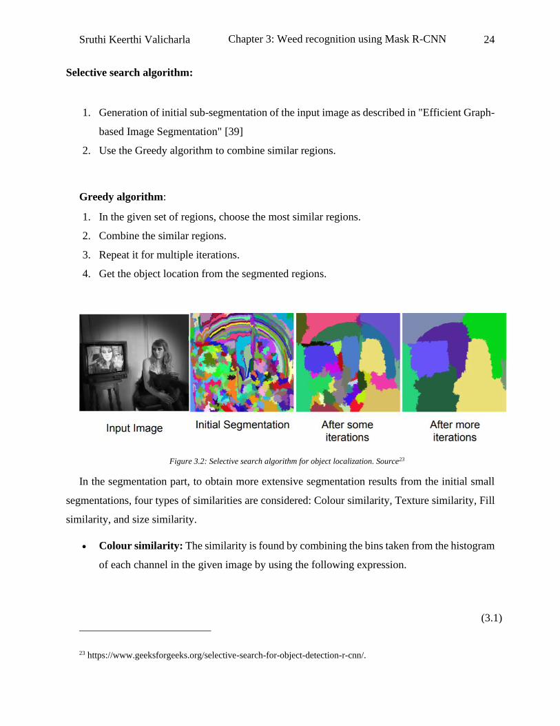
Selective search algorithm:
1. Generation of initial sub-segmentation of the input image as described in "Efficient Graph-
based Image Segmentation" [39]
2. Use the Greedy algorithm to combine similar regions.
Greedy algorithm:
1. In the given set of regions, choose the most similar regions.
2. Combine the similar regions.
3. Repeat it for multiple iterations.
4. Get the object location from the segmented regions.
Figure 3.2: Selective search algorithm for object localization. Source23
In the segmentation part, to obtain more extensive segmentation results from the initial small
segmentations, four types of similarities are considered: Colour similarity, Texture similarity, Fill
similarity, and size similarity.
• Colour similarity: The similarity is found by combining the bins taken from the histogram
of each channel in the given image by using the following expression.
23 https://www.geeksforgeeks.org/selective-search-for-object-detection-r-cnn/.
(3.1)
Chapter 3: Weed recognition using Mask R-CNN
Sruthi Keerthi Valicharla 25
𝑆𝑐𝑜𝑙𝑜𝑢𝑟(𝑟𝑖, 𝑟𝑗) = ∑ 𝑚𝑖𝑛(𝑐𝑖𝑘, 𝑐𝑗
𝑘)
𝑛
𝑘=1
cik, cj
k are the kth value of the histogram bin of region ri and rj, respectively.
• Texture similarity: The texture similarity is obtained by calculating 8 Gaussian
derivatives of the image and using ten bins for each colour channel. The histogram is
extracted by using the following formula.
𝑆𝑡𝑒𝑥𝑡𝑢𝑟𝑒(𝑟𝑖, 𝑟𝑗) = ∑ 𝑚𝑖𝑛(𝑡𝑖𝑘 , 𝑡𝑗
𝑘)
𝑛
𝑘=1
tik, tj
k are the kth value of histogram bin of region ri and rj, respectively.
• Fill similarity: The following formula is used to calculate how well the two regions fit
with one another. The condition is, if the regions fit, they should be merged else not.
Sfill(ri,rj) = 1 – (size (BBij)) – size(ri) - size(rj) / size(image)
Size (BBij) is the size of the bounding box around i and j.
• Size similarity: This feature is only considered for smaller regions to merge them easily.
If this is not done, the more prominent regions tend to combine with more significant
regions, leading to multiple scales in a specific location.
Ssize(ri,rj) = 1 – (size(ri) + size(rj)) / size(image)
Where size(ri), size(rj) and size(image) are sizes of region and image in pixels respectively.
This entire procedure of selective search is often referred to as Region Proposal. R-CNN is a
combination of Region Proposal with CNN. Usually, the CNNs run the sliding windows over the
entire image, which is computationally inefficient. However, R-CNN improves the efficiency of
computation by using only a few windows. To detect an object with R-CNN:
• Using selective search, generate category independent region proposals and warp them.
• Feed the warped region proposals to a CNN.
(3.2)
(3.3)
(3.4)
Chapter 3: Weed recognition using Mask R-CNN
Chapter 3: Weed recognition using Mask R-CNN
Sruthi Keerthi Valicharla 26
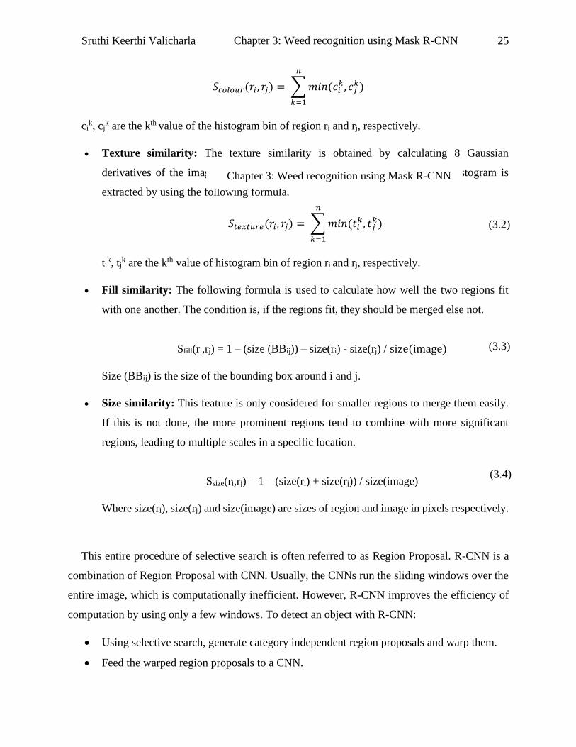
• To extract the features from the CNN, apply SVM24 as it helps classify the objects' presence
in the region. Apply Regressor to get the bounding box information.
• For all these scored regions, a non-max suppression algorithm is applied to eliminate the
intersection over union (IoU) issue by rejecting the regions with a score higher than the
threshold set while learning.
Figure 3.3: Object detection using R-CNN.
To better understand the Non-Max suppression and how it helps eliminate the multiple
detections of the same object, we need to understand IoU.
Intersection over Union:
For a given pair of bounding boxes, one obtained by the ground truth and the other from the
algorithm prediction, IoU calculates the intersection over the union of the two bounding boxes as
shown in the figure below.
24 Support Vector Machines is a supervised learning algorithm for classification and regression problem.
Chapter 3: Weed recognition using Mask R-CNN

Sruthi Keerthi Valicharla 27
(a) (b) (c)
Figure 3.4: Intersection over Union. (a) Red bounding box is ground truth and the blue bounding box is the predicted
bounding box. (b) Intersection of the bounding boxes. (c) Union of the bounding boxes.
Mathematically,
𝐼𝑜𝑈 = Area overlap between the ground truth and predicted bounding boxes
Total area of the bounding boxes
Non-max suppression usually considers the bounding boxes with IoU > 0.5 for object detection,
with IoU = 1 being that the bounding boxes are overlapping perfectly. If there are multiple
bounding boxes with IoU > 0.5, Non- Max suppression usually picks the bounding box with the
highest IoU and drops the others for the same object.
(3.5)
Chapter 3: Weed recognition using Mask R-CNN
Sruthi Keerthi Valicharla 28
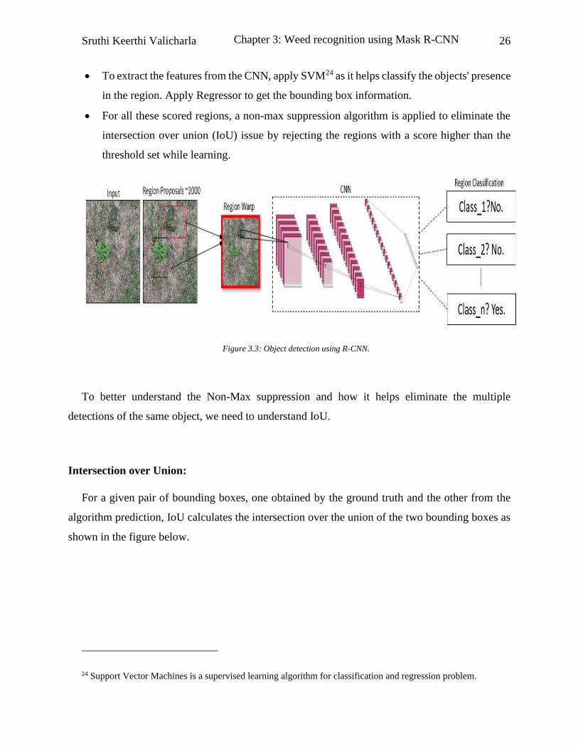
The architecture of R-CNN:
Figure 3.5: The network architecture of R-CNN.
The workflow is as follows:
1. The input image is fed to a selective search block to get the 2000 region proposals.
2. These warped region proposals are fed through CNNs to extract the features.
3. The extracted features are sent through SVM for object identification and a Regression
block to get the bounding boxes.
Drawbacks of R-CNN:
Computationally inefficient as we must use 2000 region proposals for each image. So, for X
images, the total number of CNN features would be X*2000. These region proposals make the
training slow.
To overcome this, we can use ConvNets instead of 2000 region proposals per image. We can
also combine the feature extraction, classifier, and bounding box generator blocks. All of this is
done in Fast R-CNN.
Fast R-CNN:
As the name indicates, Fast R-CNN [40] is a fast framework that uses a CNN to extract the
entire image's features instead of 2000 region proposals per image for object recognition in an
image.
Chapter 3: Weed recognition using Mask R-CNN

Sruthi Keerthi Valicharla 29
The architecture of Fast R-CNN:
Figure 3.6: The network architecture of Fast R-CNN.
The workflow is as follows:
1. The input image features are extracted using a single CNN.
2. We have an RoI (Region of Interest) pooling block that extracts the fixed-length feature
vector from the feature map obtained from the max pooling25 layers of the input image.
3. The feature vector obtained from RoI pooling is then fed to Fully Connected (FC) layers
of a neural network. However, as the FC network needs a fixed size image as an input, we
need to warp the patches of the feature maps extracted from the previous step.
4. The FC network will then perform the localization and classification task.
5. The final output layers of the FC network are Softmax and Regressor. Softmax is a
probability block that estimates the object classes and the background, which is a class.
Regressor, on the other hand, will give the bounding box information.
25 Finding the maximum value in each feature map’s patch
Chapter 3: Weed recognition using Mask R-CNN

Sruthi Keerthi Valicharla 30
The detection quality is improved because it uses Softmax over SVM as a classifier and the
training is single-stage, and training updates all the network layers. Softmax outperforms SVM as
it gives the probability for each class while SVM, on the other hand, will be least concerned about
the other classes. Hence, SVM is generally helpful if we have a single class classification problem.
Drawbacks of Fast R-CNN:
Although the performance of Fast R-CNN is improved by using a deep CNN for feature
extraction, the selective search for RoI is still expensive computationally when it comes to large
real-time datasets. So, the selective search approach for RoI selection can be replaced with another
CNN. This limitation gives rise to Faster R-CNN [41].
Faster R-CNN:
Faster R-CNN's performance is faster than fast R-CNN because it is a single unified network
for the object detection problem. It just has a CNN for RoI extraction, referred to as Region
Proposal Network (RPN) and the Fast R-CNN model. RPN shares the computation along with the
Fast R-CNN block.
The architecture of Faster R-CNN:
Figure 3.7: The network architecture of Faster R-CNN.
Chapter 3: Weed recognition using Mask R-CNN

Sruthi Keerthi Valicharla 31
To understand the Faster R-CNN workflow, we need to understand the Region Proposal
Network (RPN) architecture.
RPN:
RPN is used for the region proposal task in Faster R-CNN. RPN has a unique architecture as it
contains regressors and classifiers. The RPN input is an image with an unfixed size, and the output
of RPN is a bunch of object proposals, each with an object score. The object proposals are obtained
by sliding a little network over the CNN layer's feature map. These object proposals are then fed
to two sibling-connected layers: The Classifier - for object identification and the Regressor - for
bounding box creation. The architecture of the RPN is shown below.
Figure 3.8: Working of RPN. Source [33]
Another critical term that needs to be understood is Anchor. An anchor is placed at the midpoint
of the sliding window associated with a scale and aspect ratio. Anchors help with translational
invariance that was mentioned earlier. The number of anchors for each sliding window for Faster
R-CNN is nine as it uses three scales and three aspect ratios. With these anchors, we can predict
multiple region proposals at every sliding window location, with k being the maximum number of
proposals for that location. The object score can be calculated using these k values. The regression
layer outputs 4-k outputs to get the bounding box coordinates, and the classifier layer outputs 2-k
Chapter 3: Weed recognition using Mask R-CNN

Sruthi Keerthi Valicharla 32
scores, which will provide the information about the probability of the object present and absent
in each region proposal. The number of anchors can be calculated by W*H*k, with W and H being
the width and height of the image. As this algorithm is robust against translations, translation
invariance can be achieved. The anchors get their labels based on two factors: anchors with the
highest IoU overlapping with ground truth and anchors with IoU > 0.7.
All in all, the Faster R-CNN model uses three different neural networks: a Feature Network to
extract the feature maps from the given input image, an RPN for getting the RoIs with the highest
object containing probability, and finally, a Detection Network for generating the bounding boxes
and class of the object. Faster R- CNN can be used for other tasks like image captioning, instance
segmentation, 3-D object detection.
To perform instance segmentation, we need to identify each object instance of every known
object in an image. So, Faster R-CNN is further extended to Mask R-CNN.
Mask R-CNN:
Instance segmentation is generally used for counting objects in an image. Instance segmentation
usually assigns a label to each pixel in the image. It is more like pixel-level classification. Along
with the boundary box creation around the object, we need a segmentation mask around the desired
object for the instance segmentation.
Chapter 3: Weed recognition using Mask R-CNN

Sruthi Keerthi Valicharla 33
3.2: Network architecture:
Figure 3.9: The network architecture of Mask R-CNN.
The workflow is as follows:
1. Mask R-CNN has an additional Binary mask classifier block along with the RPN stage as
in Faster R-CNN. This block generates masks for every class in the image, and the RPN
will give the bounding box details.
2. Every image then goes through a CNN to generate multiple RoI using the mask classifier
to obtain the feature maps.
3. The RPN block uses Non-Max suppression to get the nine anchors' highest object scores.
4. Mask R-CNN uses an RoI align network to get multiple bounding boxes around an object
and warps it to a single dimension.
5. As in Faster R-CNN, these warped features are fed to an FC network to obtain the object
class and the bounding box from Softmax and regressor blocks, respectively.
6. Along with the FC network, the warped features are fed to the Mask Classifier block, which
uses multiple CNNs to generate the masks around every class's objects.
Chapter 3: Weed recognition using Mask R-CNN

Sruthi Keerthi Valicharla 34
3.3: Feature extraction with Feature Pyramid Network:
Detection of objects using multi-scale images for a small object is challenging. We can resolve
this problem by using a pyramid of the same image to detect the object, but it is very time-
consuming. We can use this approach when speed is not a requirement. On the other hand, we can
use a pyramid of features to extract the objects' information (right-side image). However, this
method will not provide accurate object detection.
(a) (b)
Figure 3.10: Pyramid architecture. (a) Pyramid of images. (b) Pyramid of feature maps. Source [42]
Feature Pyramid Network (FPN) [42] is designed to address the accuracy and speed limitation
issues. FPN can be replaced with the traditional feature extractors to obtain multiple feature maps,
which provide better quality feature information. FPN has both bottom-up and top-down pathways.
The dataflow looks as follows:
Figure 3.11: Dataflow in an FPN. Source [42]
Chapter 3: Weed recognition using Mask R-CNN
Sruthi Keerthi Valicharla 35
As we proceed from the top to bottom layers, the image's spatial resolution increases, and the
semantic value decreases. The bottom-up pathway is the standard feature extractors used in CNNs.
The top-down pathway is used for Mask R-CNN. It provides a combination of low-resolution
semantically robust features with high resolution semantically weak features. FPN grabs all the
semantic features from a single scale, therefore, avoiding problems like power consumption and
memory.
FPN for RPN:
Initially, the RPN in Faster R-CNN used a 3x3 sliding window CNN to obtain the bounding
box regions and the object classification information. If we replace this conventional technique
with FPN, we will no longer be required to have anchors at multi-scales. At each level, multiple
aspect ratios are used. Hence, the anchors will be assigned a positive value only if the IoU is 70%.
On the other hand, the anchors will have a negative label if the IoU is < 30%. RoIs of different
scales must be fed to the pyramid levels to detect an object in an image.
ResNet 101 Backbone:
A residual neural network (ResNet) [43] is one of the Artificial Neural Networks (ANNs) that
builds on pyramid cells. A conventional ResNet consists of layers of ReLUs aided by batch
normalization. Unlike in general CNNs, the residual networks learn residue instead of learning
low, mid, and high-level features. Residual of each layer is defined as the subtraction of features
learned from the input of that layer. These residual layers help simplify the training process and
helps with the degrading accuracy [44] problem because as the depth of the network increases, the
accuracy is saturating and starts degrading. There are multiple variants of the residual network,
including but not limited to ResNet50, ResNet100, ResNet152.
Chapter 3: Weed recognition using Mask R-CNN
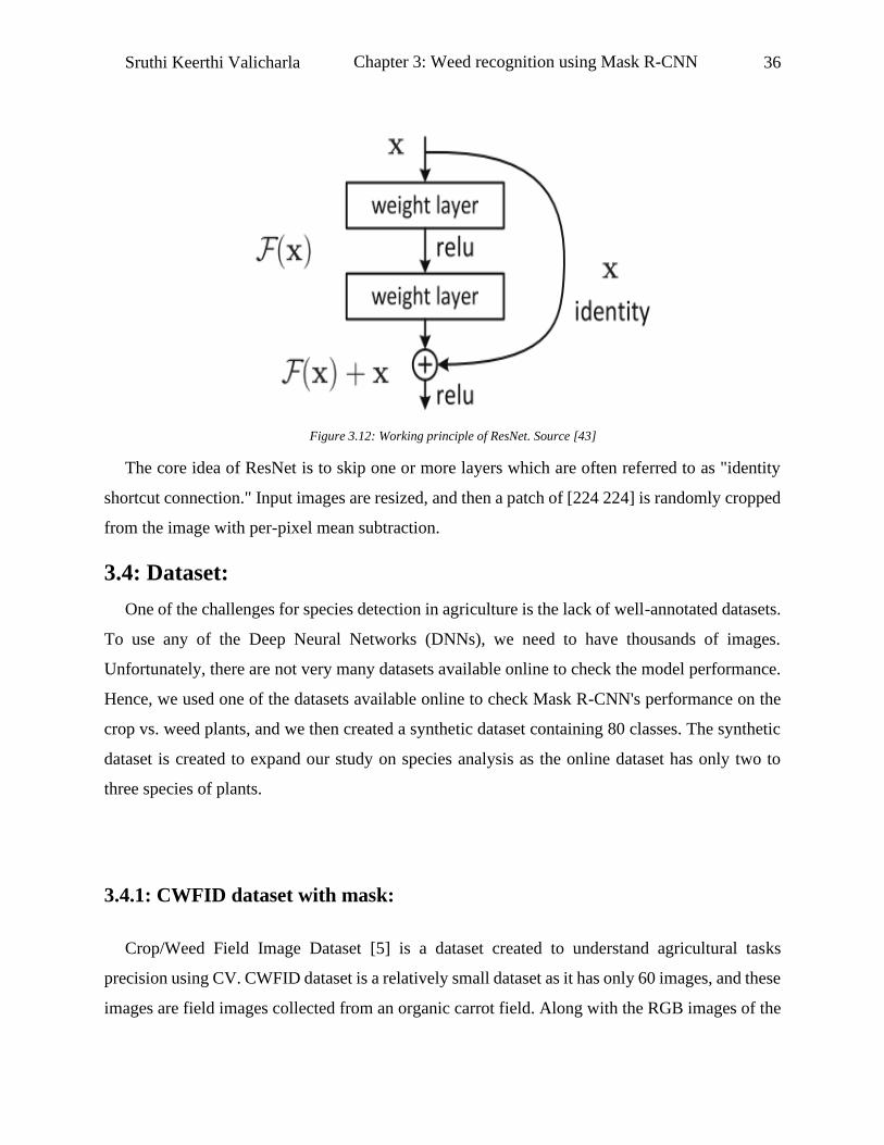
Sruthi Keerthi Valicharla 36
Figure 3.12: Working principle of ResNet. Source [43]
The core idea of ResNet is to skip one or more layers which are often referred to as "identity
shortcut connection." Input images are resized, and then a patch of [224 224] is randomly cropped
from the image with per-pixel mean subtraction.
3.4: Dataset:
One of the challenges for species detection in agriculture is the lack of well-annotated datasets.
To use any of the Deep Neural Networks (DNNs), we need to have thousands of images.
Unfortunately, there are not very many datasets available online to check the model performance.
Hence, we used one of the datasets available online to check Mask R-CNN's performance on the
crop vs. weed plants, and we then created a synthetic dataset containing 80 classes. The synthetic
dataset is created to expand our study on species analysis as the online dataset has only two to
three species of plants.
3.4.1: CWFID dataset with mask:
Crop/Weed Field Image Dataset [5] is a dataset created to understand agricultural tasks
precision using CV. CWFID dataset is a relatively small dataset as it has only 60 images, and these
images are field images collected from an organic carrot field. Along with the RGB images of the
Chapter 3: Weed recognition using Mask R-CNN

Sruthi Keerthi Valicharla 37
size 640 x 480, the vegetation masks were also provided. These masks help to create an annotation.
The 60 images were split into 48 training images and 12 testing/validation images to maintain the
split ratio of 4:1. To train the Mask R-CNN, we need to have more than 60 images to get better
results. So, we have used a data augmentation technique that is explained in section 4.3. We have
generated 2064 training images and 516 testing images. The images below are an example of the
RGB image and the annotated mask.
(a) (b)
Figure 3.13: Images from CWFID. (a) RGB image of weed and crop plants. (b) Annotated image with the red colour being
the weed plant and green colour being the carrot crop plant. Source [5]
The image on the right side is the annotated mask with the red colour as the weed plant and the
green colour as the crop plant. In this section, we will be using Mask R-CNN with MS COCO [32]
weights. Hence, we converted this small dataset into a coco format, meaning creating the JSON
file for all annotations.
The annotation part provides the information about the bounding boxes from the segmented
mask. The iscrowd field determines the nature of the object, with iscrowd = 0 being an individual
object and iscrowd = 1 being a crowd like a crowd of people in a stadium. The category id field
will provide the information of the category and the super-category details. Segmentation is
usually Polygon, with x, y being the top-left point and width and height being the bounding box's
Chapter 3: Weed recognition using Mask R-CNN

Sruthi Keerthi Valicharla 38
size. Run-Length Encoding or RLE is used to separate the foreground and background in an image
and is generally used if iscrowd = 1.
We have generated the bounding boxes for our COCO type CWFID dataset by using the
predefined mask definitions. The masks are defined based on the red and green colours. The red
colour (255,0,0) is considered a weed plant, and the green colour (0, 255, 0) is the crop plant. As
there are only two classes, the super-category is fixed to Plant.
Figure 3.14: Example images from the COCO type CWFID dataset.
Limitations:
This dataset's drawbacks are that it considers all the weed plants as a single class, and the crop
plants also fall under one species, to be precise, organic carrot. To test the performance of Mask
R-CNN for multiple classes, we created a synthetic dataset with 80 classes in it.
3.4.2: Synthetic COCO dataset:
In this dataset, we created images with multiple plants in them. We have used 80 foreground
images of weed plants26 and a few background images as shown below:
26 https://www.immersivelimit.com/course/creating-coco-datasets.
Chapter 3: Weed recognition using Mask R-CNN

Sruthi Keerthi Valicharla 39
(a)
(b)
Figure 3.15: Types of images used for creating the synthetic data with 80 classes. (a) Foreground examples. (b) Background
examples.
As we are currently unaware of these species' names, we named our plants class_1 to class_80.
Using random placements, we have placed these foreground images on the background images.
The masks were created using the alpha layer of the foreground images. We have generated the
COCO JSON file using the masks to get the details about the bounding boxes. The iscrowd is set
to 0, and the super-category is set as weeds.
We have generated 10000 training images and 2500 testing images. Although the number can
be increased, we set it low just to check if the model can detect the classes or not. With the masks
and the annotations, the synthetic images look like the following:
Chapter 3: Weed recognition using Mask R-CNN

Sruthi Keerthi Valicharla 40
Figure 3.16: Example image from the COCO type Synthetic dataset.
Dataset Comparison:
Dataset Number of
Images
Number of
Classes
Task Channel Size Labels
Plant -
Seedling
960 12 Segmentation RGB Variable 960
Agriculture-
Vision [6]
96,984 6 Segmentation
(aerial)
RGB, NIR 512 x 512 168,086
Dataset of
Tomato leaves
[9]
14,531 10 Classification RGB 227 x 227 14,531
100 leaves
plant species
[8]
1,000 16 Classification Binary variable 1,600
DeepWeeds
[12]
17,509 8 Classification RGB 256 x 256 17,509
CWFID [5] 60 2 Segmentation RGB 640 x 480 494
Our Synthetic
data
12,500 80 Segmentation RGB 1000 x 1000 19,963
Table 1: Statistical comparison between other datasets and our synthetic dataset
Chapter 3: Weed recognition using Mask R-CNN
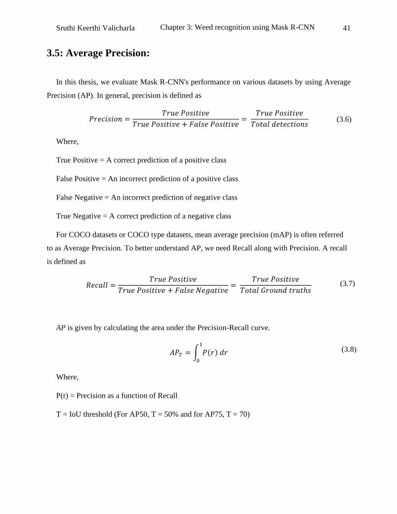
Sruthi Keerthi Valicharla 41
3.5: Average Precision:
In this thesis, we evaluate Mask R-CNN's performance on various datasets by using Average
Precision (AP). In general, precision is defined as
𝑃𝑟𝑒𝑐𝑖𝑠𝑖𝑜𝑛 =𝑇𝑟𝑢𝑒 𝑃𝑜𝑠𝑖𝑡𝑖𝑣𝑒
𝑇𝑟𝑢𝑒 𝑃𝑜𝑠𝑖𝑡𝑖𝑣𝑒 + 𝐹𝑎𝑙𝑠𝑒 𝑃𝑜𝑠𝑖𝑡𝑖𝑣𝑒=
𝑇𝑟𝑢𝑒 𝑃𝑜𝑠𝑖𝑡𝑖𝑣𝑒
𝑇𝑜𝑡𝑎𝑙 𝑑𝑒𝑡𝑒𝑐𝑡𝑖𝑜𝑛𝑠
Where,
True Positive = A correct prediction of a positive class
False Positive = An incorrect prediction of a positive class
False Negative = An incorrect prediction of negative class
True Negative = A correct prediction of a negative class
For COCO datasets or COCO type datasets, mean average precision (mAP) is often referred
to as Average Precision. To better understand AP, we need Recall along with Precision. A recall
is defined as
𝑅𝑒𝑐𝑎𝑙𝑙 =𝑇𝑟𝑢𝑒 𝑃𝑜𝑠𝑖𝑡𝑖𝑣𝑒
𝑇𝑟𝑢𝑒 𝑃𝑜𝑠𝑖𝑡𝑖𝑣𝑒 + 𝐹𝑎𝑙𝑠𝑒 𝑁𝑒𝑔𝑎𝑡𝑖𝑣𝑒=
𝑇𝑟𝑢𝑒 𝑃𝑜𝑠𝑖𝑡𝑖𝑣𝑒
𝑇𝑜𝑡𝑎𝑙 𝐺𝑟𝑜𝑢𝑛𝑑 𝑡𝑟𝑢𝑡ℎ𝑠
AP is given by calculating the area under the Precision-Recall curve.
𝐴𝑃𝑇 = ∫ 𝑃(𝑟) 𝑑𝑟1
0
Where,
P(r) = Precision as a function of Recall
T = IoU threshold (For AP50, T = 50% and for AP75, T = 70)
(3.6)
(3.7)
(3.8)
Chapter 3: Weed recognition using Mask R-CNN

Sruthi Keerthi Valicharla 42
Figure 3.17: IoU = 0.5 (left), IoU= 0.75 (right)
AP for a class,
𝐴𝑃[𝑐𝑙𝑎𝑠𝑠] = 1
𝐷𝑖𝑓𝑓𝑒𝑟𝑒𝑛𝑡 𝑇ℎ𝑟𝑒𝑠ℎ𝑜𝑙𝑑𝑠∑ 𝐴𝑃(𝑐𝑙𝑎𝑠𝑠, 𝐼𝑜𝑈)
AP for all classes,
𝐴𝑃 = 1
𝐴𝑙𝑙 𝐶𝑙𝑎𝑠𝑠𝑒𝑠∑ 𝐴𝑃(𝑐𝑙𝑎𝑠𝑠)
Therefore, AP50 = AP at IoU @ 0.5 and AP75 = AP at IoU @ 0.75.
3.6: Experiment setup:
3.6.1 Using CWFID:
Using the Mask R-CNN model to detect the crop vs. weed plants, we have used Resnet 50 FPN
as a backbone for feature extraction. The learning rate used is 0.001, and the number of epochs is
1000. The batch size is 4, and the number of classes is 3 (crop, weed, and background). We used
Detectron2 to conduct this experiment.
Chapter 3: Weed recognition using Mask R-CNN
(3.9)
(3.10)

Sruthi Keerthi Valicharla 43
3.6.2 Using Synthetic COCO dataset:
The experiment setup is the same with some slight modifications. The batch size is 2, and the
number of classes would be 81 (80 weed classes and one background class).
3.7: Results and Discussion:
CWFID: As the dataset is good enough for 2 class information, we have set the Softmax
threshold to 0.9. The results are as follows:
Figure 3.18: COCO type CWFID’s Mask R-CNN results with Softmax threshold = 0.9. The number on the top of the
bounding box is the probability of the plant being a specific class like Crop_Plant or Weed_Plant.
Synthetic COCO dataset: The dataset created is minimal for an 80-classes classifier. The
original COCO dataset has 2,500,000 labelled images for 80 classes. The comparison of
performance is not possible due to a lack of enough information with our dataset. Ideally, 1000
images per class are preferred. We have set the Softmax threshold to 0.5.
Chapter 3: Weed recognition using Mask R-CNN

Sruthi Keerthi Valicharla 44
Figure 3.19: Synthetic COCO dataset’s Mask R-CNN results with Softmax threshold = 0.5. The number on the top of the
bounding box is the probability of the plant being a specific class like Class_1 – Class_80.
Discussion:
To analyse Mask R-CNN's performance, we adjusted the synthetic dataset to 2 classes, one crop
plant and the rest as weed plants, and reduced the number of images to 1250. This dataset is still
an advancement over CWFID as CWFID has only two types of weeds, and we have ~75 weed
types in our weed class.
Dataset # images # Classes AP AP5027
CWFID [5] 60 2 79.6 NA
Adjusted Synthetic data 1250 2 50.03 75.952
Table 2: Comparison of Mask R-CNN’s performance on ground-level plant recognition image with CWFID.
Our adjusted synthetic data was able to reach ~50% accuracy. Nevertheless, it can be improved
with more crop species and thereby avoiding the data imbalance28 problem.
As we do not have enough information about the weed plant species, our 80-class dataset might
even have redundant species in them. Despite all these limitations, Mask R-CNN was able to
27 Average precision at IoU = 0.5 28 Image distribution among the classes is skewed (biased).
Chapter 3: Weed recognition using Mask R-CNN

Sruthi Keerthi Valicharla 45
localize the plants on a given image. To progress our study on MAM (see chapter 5), we need to
have sufficient data to test it with Mask R-CNN.
Chapter 3: Weed recognition using Mask R-CNN
Sruthi Keerthi Valicharla 46
Chapter 4:
Data Augmentation for Aerial Images:
4.1 Introduction:
When we consider the most popular datasets, the number of images ranges from thousands or
tens of thousands or even millions. For getting an improved performance of the CNN, we need to
have large datasets. Data Augmentation is a technique used to increase the number of data points
or images in our case by adding the slightly altered copies of available limited data or creating new
synthetic data as mentioned in section 3.4.2. By doing this data augmentation, we can reduce the
problem of overfitting while training a neural network. When we train a DNN or any other machine
learning model, we are tuning the model's parameters to map an image input to a label output with
a goal to reduce the model loss. The current State-of-the-art (SOTA) CNNs have millions of
parameters. It is only logical to have a proportionate number of images to obtain decent
performance. As most object recognition or localization algorithms exhibit translational invariance
(section 3.1), this property will serve as a baseline for the data augmentation. Data augmentation
can be as simple as flipping the images, changing the image's orientation, or changing its scale or
brightness. Data augmentation will be helpful even if we have a large amount of data as well. For
instance, in the synthetic data created in section 3.4.2, if all of the class_1 species are left-aligned
and class_2 species are right-aligned, the model is likely to get confused when we provide class_1
species that is right-aligned, although if the model has a 90% accuracy. It is because the model
will learn that all left-aligned will most likely be class_1. Hence, if we use data augmentation, this

Sruthi Keerthi Valicharla 47
problem can be solved. There are multiple options to achieve this data augmentation. Some of
them are:
1. Neural Style Transfer
2. Geometrical transformations
4.2 Style Transfer:
4.2.1 Introduction:
Usage of Neural Style Transfer is an advanced technique for data augmentation as it focuses on
the colour, the texture of the image and addresses illumination variation problems, unlike
conventional data augmentation techniques such as flipping, cropping, and rotation. NST will be
a good choice if we consider the semantic content of the image with translational invariance. As
we need thousands of images for our weed detection, we created a dataset using the localized style
transfer technique.
4.2.2 Localized Style Transfer:
As mentioned in section 2.2.2, we have used localized style transfer to transfer the Mile-A-
Minute style from the images we have collected to some aerial images obtained from the
Agriculture - Vision 2020 dataset [6]. These images are taken from various farmlands across the
United States to address semantic segmentation in agriculture. These images are of exceptional
quality, and they are well annotated. Compared to other agriculture datasets, this dataset has a
relatively high number of images in RGB and NIR29 channels. As most object recognition datasets
focus on everyday objects, it is challenging to understand agriculture images' patterns without
proper datasets. As we focus on MAM recognition using UAVs, we need more images to train our
neural networks effectively. To address this issue, we used a localized style transfer technique
using CNN [45]. In general, the content loss function and style loss functions play a crucial role in
29 Near Infra-Red
Chapter 4: Data Augmentation for Aerial Images

Sruthi Keerthi Valicharla 48
NST. We adjust the style loss function in the localized style transfer technique to apply the style
to masked regions. In this thesis, we used VGG19 to achieve our goal of creating synthetic data.
4.2.3 VGG19 network Architecture:
As the name suggests, VGG19 has 19 layers to extract the features from a given image. This
network has been trained on the ImageNet dataset [46]. The shallow layers of this network focus
on the pixel-level information while the deep layers, on the other hand, focus on the object
localization. VGG19 is a variant of VGG developed by Visual Geometry Group. Some of the other
available variants of VGG are VGG11, VGG16, VGG19. The VGG architecture outperformed
many SOTA models for ImageNet Large-Scale Visual Recognition Challenge (ILSVRC). As
ImageNet is a classifier dataset, in simple terms, VGG is an image classifier CNN. The architecture
of VGG19 is as follows.
Figure 4.1: The network architecture of VGG19.
The workflow is as follows:
1. An RGB image of size 224x224 is given as an input to the network. The input image size
is fixed, thereby leading to a fixed shape of (224,224,3).
2. The mean RGB value is subtracted from every pixel as pre-processing.
3. A kernel of size 3x3 is used to slide over the entire image with a stride of 1.
Chapter 4: Data Augmentation for Aerial Images

Sruthi Keerthi Valicharla 49
4. Spatial padding is done to preserve the spatial resolution of the input image.
5. Down-sampling is done by using max pooling with a window size of 2x2 and stride 2.
6. ReLu units are introduced to improve computational efficiency and classification
efficiency. As discussed in section 3.1, ReLu is a better activation function choice than
sigmoid functions or hyperbolic tangents.
7. The images are then fed to three FC layers. As shown in the below table, the first two FCs
have a size of 4096, and the third FC has a size of 1000. The ReLu layers are not mentioned
in the table below to avoid complexity.
8. The final layer of VGG19 is a Softmax function to provide the probability of the
classification.
ConvNet Configuration of VGG19
19 weight layers
224x224 Input Image (RGB)
Conv3-64
Conv3-64
Max pooling
Conv3-128
Conv3-128
Max pooling
Conv3-256
Conv3-256
Conv3-256
Conv3-256
Max pooling
Chapter 4: Data Augmentation for Aerial Images
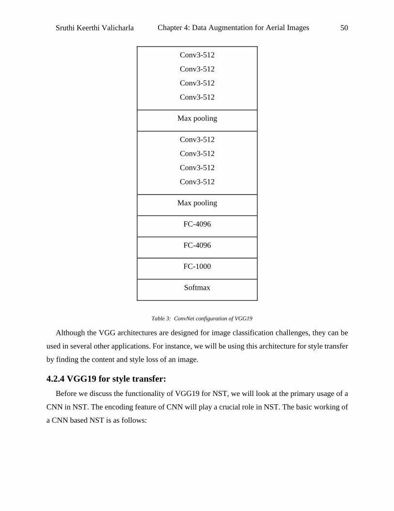
Sruthi Keerthi Valicharla 50
Conv3-512
Conv3-512
Conv3-512
Conv3-512
Max pooling
Conv3-512
Conv3-512
Conv3-512
Conv3-512
Max pooling
FC-4096
FC-4096
FC-1000
Softmax
Table 3: ConvNet configuration of VGG19
Although the VGG architectures are designed for image classification challenges, they can be
used in several other applications. For instance, we will be using this architecture for style transfer
by finding the content and style loss of an image.
4.2.4 VGG19 for style transfer:
Before we discuss the functionality of VGG19 for NST, we will look at the primary usage of a
CNN in NST. The encoding feature of CNN will play a crucial role in NST. The basic working of
a CNN based NST is as follows:
Chapter 4: Data Augmentation for Aerial Images

Sruthi Keerthi Valicharla 51
Figure 4.2: Concept of NST with CNN.
We have a noisy input image fed to the CNN to serve as our output image. Along with the input
image, we have a content image (C), and a style image (S) fed to CNN. Our objective is to find
how identical is our input image to the content and style images, respectively, at every layer in the
VGG. We need to preserve the content of the content image and the style of the style image. So,
we define and calculate the content and style loss as follows:
Content loss:
This measure gives us the similarity quotient of our noisy input image with the content image
at a given layer (L) in VGG. If P and F are the original and generated images, F(1) and P(1) are
their L layer values. The content loss is given as:
Lcontent = 1
2 ∑ (𝐹𝑖𝑗
𝑙 − 𝑃𝑖𝑗 𝑙 )2
𝑖,𝑗
Style Loss:
To understand the style loss, we need to have a better understanding of the term style. The style
information is calculated by using the correlation value of the feature maps in a layer. The loss
function is obtained by taking the difference between feature maps produced by the style image
and the generated image.
(4.1)
Chapter 4: Data Augmentation for Aerial Images
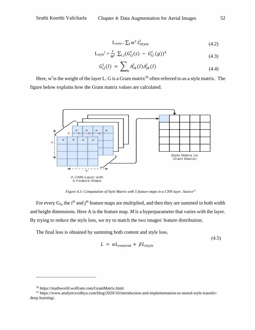
Sruthi Keerthi Valicharla 52
Lstyle = ∑ 𝑤𝑙 𝐿𝑠𝑡𝑦𝑙𝑒𝑙
𝑙
Lstylel =
1
𝑀𝑙 ∑ (𝐺𝑖𝑗𝑙 (𝑠) − 𝐺𝑖𝑗
𝑙 (𝑔))2𝑖,𝑗
𝐺𝑖𝑗𝑙 (𝐼) = ∑ 𝐴𝑖𝑘
𝑙 (𝐼)𝐴𝑗𝑘𝑙 (𝐼)
𝑘
Here, wl is the weight of the layer L. G is a Gram matrix30 often referred to as a style matrix. The
figure below explains how the Gram matrix values are calculated.
Figure 4.3: Computation of Style Matrix with 5 feature maps in a CNN layer. Source31
For every Gij, the ith and jth feature maps are multiplied, and then they are summed in both width
and height dimensions. Here A is the feature map. M is a hyperparameter that varies with the layer.
By trying to reduce the style loss, we try to match the two images' feature distribution.
The final loss is obtained by summing both content and style loss.
𝐿 = 𝛼𝐿𝑐𝑜𝑛𝑡𝑒𝑛𝑡 + 𝛽𝐿𝑠𝑡𝑦𝑙𝑒
30 https://mathworld.wolfram.com/GramMatrix.html. 31 https://www.analyticsvidhya.com/blog/2020/10/introduction-and-implementation-to-neural-style-transfer-
deep-learning/.
(4.2)
(4.3)
(4.4)
(4.5)
Chapter 4: Data Augmentation for Aerial Images

Sruthi Keerthi Valicharla 53
Here, α and 𝛽 are user-defined parameters to adjust the amount of content and style loss that
needs to be injected into the final generated image.
There are multiple options for us to use this NST. We can transfer the style without colour,
texture transfer to the entire image, or segmented image. We have used the last option. Here are
the examples of each case.
Technique Content Image Style Image Generated Image
Style
and Colour
transfer
Style
transfer
Table 4: Illustration of Global style transfer with and without colour transfer from the style image to the content image.
Chapter 4: Data Augmentation for Aerial Images

Sruthi Keerthi Valicharla 54
(a) (b) (c)
Figure 4.4: An example of localized style transfer. (a) content image, (b) Mask of the content image, (c) Generated image
with a random style. Source [6]
As we want to perform the style transfer with semantic segmentation, we need to modify the
style loss function to transfer only to the RoI.
Algorithm for semantic segmentation style transfer [47] :
1. Take patches from the semantic layer or the mask for both style and generated images.
2. Find the nearest neighbour for a given patch in a layer by finding the cross-correlation.
𝑁𝑁(𝑖) = 𝑎𝑟𝑔𝑗𝑚𝑖𝑛Ψ𝑠(𝑠). Ψ𝑗(𝑠𝑠)
|Ψ𝑠(𝑠)|. |Ψ𝑗(𝑠𝑠)|
3. The style error between all the patches and the generated image in that particular layer can
be calculated by finding the Euclidean distances' summation [Reference].
𝐸𝑠(𝑠, 𝑠𝑠) = ∑ ||Ψ𝑠(𝑠) − Ψ𝑁𝑁(𝑖)(𝑠𝑠)|| 2𝑖
4.2.5 Hyperparameters:
The hyperparameters α and 𝛽 helps to determine the amount of style that needs to be transferred
with a minimum loss. The content weight (α) value chosen for our dataset creation is 5e0, and the
(4.6)
(4.7)
Chapter 4: Data Augmentation for Aerial Images
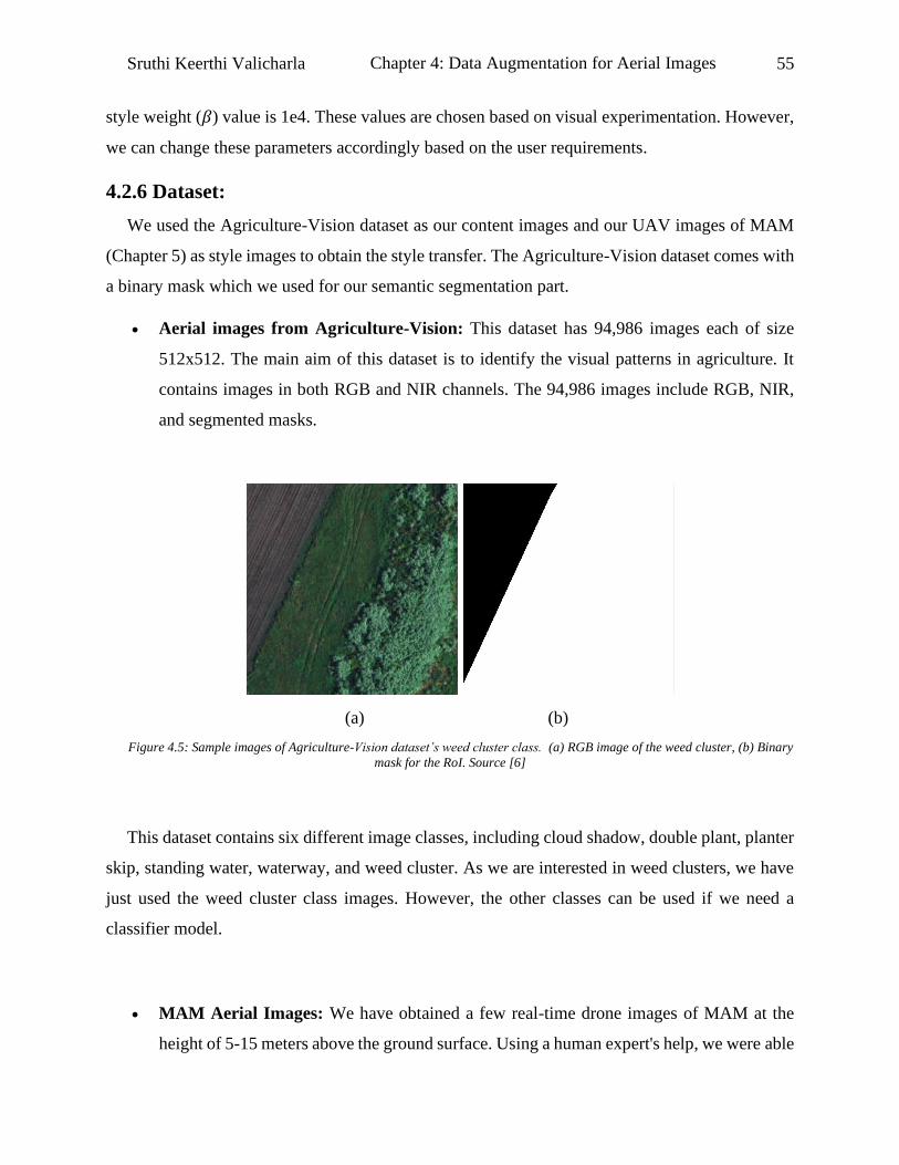
Sruthi Keerthi Valicharla 55
style weight (𝛽) value is 1e4. These values are chosen based on visual experimentation. However,
we can change these parameters accordingly based on the user requirements.
4.2.6 Dataset:
We used the Agriculture-Vision dataset as our content images and our UAV images of MAM
(Chapter 5) as style images to obtain the style transfer. The Agriculture-Vision dataset comes with
a binary mask which we used for our semantic segmentation part.
• Aerial images from Agriculture-Vision: This dataset has 94,986 images each of size
512x512. The main aim of this dataset is to identify the visual patterns in agriculture. It
contains images in both RGB and NIR channels. The 94,986 images include RGB, NIR,
and segmented masks.
(a) (b)
Figure 4.5: Sample images of Agriculture-Vision dataset’s weed cluster class. (a) RGB image of the weed cluster, (b) Binary
mask for the RoI. Source [6]
This dataset contains six different image classes, including cloud shadow, double plant, planter
skip, standing water, waterway, and weed cluster. As we are interested in weed clusters, we have
just used the weed cluster class images. However, the other classes can be used if we need a
classifier model.
• MAM Aerial Images: We have obtained a few real-time drone images of MAM at the
height of 5-15 meters above the ground surface. Using a human expert's help, we were able
Chapter 4: Data Augmentation for Aerial Images

Sruthi Keerthi Valicharla 56
to get MAM boundaries for 15 images. The image size is 5472 x 3648 as these images are
taken using a high-quality camera. Since the image size is huge, we need to resize it to
avoid crashing the deep learning model and incorporate the 512 x 512 Agriculture-Vision
dataset. The red boundaries shown below are human-made, and they provide information
about the MAM.
Figure 4.6: Real-time MAM aerial images with manually marked MAM regions.
In this thesis, we have used these MAM images to serve as our style images, and their style is
imposed on the weed cluster images of the Agriculture Vision Dataset.
4.2.7 Experiment setup:
This section will focus on the experiment setup for our localized style transfer data
augmentation. The hyperparameters details are mentioned in section 4.2.4, and the VGG19
network is initialized by using the content image (in our case Agriculture-Vision Images). The
Chapter 4: Data Augmentation for Aerial Images
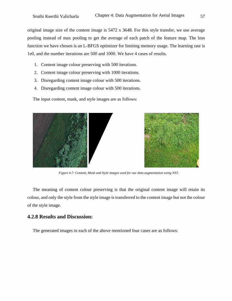
Sruthi Keerthi Valicharla 57
original image size of the content image is 5472 x 3648. For this style transfer, we use average
pooling instead of max pooling to get the average of each patch of the feature map. The loss
function we have chosen is an L-BFGS optimizer for limiting memory usage. The learning rate is
1e0, and the number iterations are 500 and 1000. We have 4 cases of results.
1. Content image colour preserving with 500 iterations.
2. Content image colour preserving with 1000 iterations.
3. Disregarding content image colour with 500 iterations.
4. Disregarding content image colour with 500 iterations.
The input content, mask, and style images are as follows:
Figure 4.7: Content, Mask and Style images used for our data augmentation using NST.
The meaning of content colour preserving is that the original content image will retain its
colour, and only the style from the style image is transferred to the content image but not the colour
of the style image.
4.2.8 Results and Discussion:
The generated images in each of the above mentioned four cases are as follows:
Chapter 4: Data Augmentation for Aerial Images
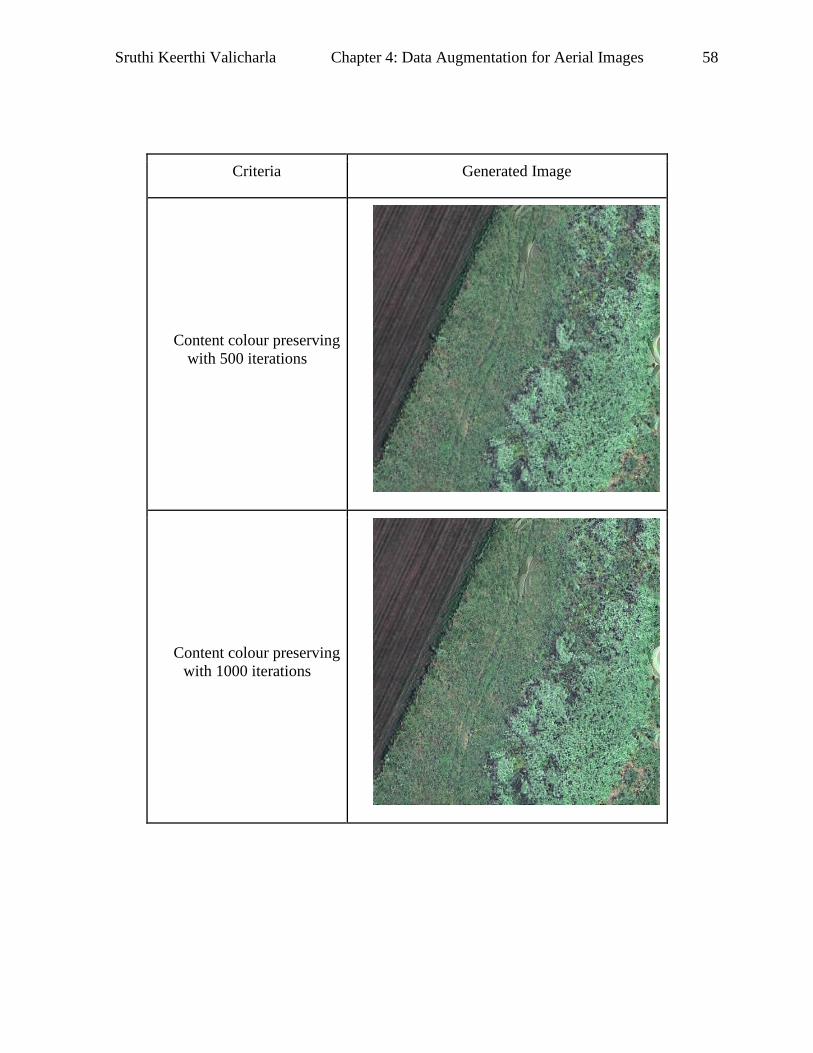
Sruthi Keerthi Valicharla 58
Criteria Generated Image
Content colour preserving
with 500 iterations
Content colour preserving
with 1000 iterations
Chapter 4: Data Augmentation for Aerial Images

Sruthi Keerthi Valicharla 59
No content colour
preserving with 500
iterations
No content colour
preserving with 1000
iterations
Table 5: Results of our NST data augmentation with VGG19
Discussion:
One of the pros of using NST for our data augmentation is that we can have various colour
variations in our plant dataset and increase the number of images. The major con is that as we keep
increasing the number of iterations, the images are looking more artistic than realistic, making it
very hard for any model to understand the underlying patterns in the image. Without these pattern
identifications, we cannot determine the species of the plants. The other con is that each image
needs at least 1-2 minutes to go through the VGG 19. To produce a decent dataset, we need a
Chapter 4: Data Augmentation for Aerial Images
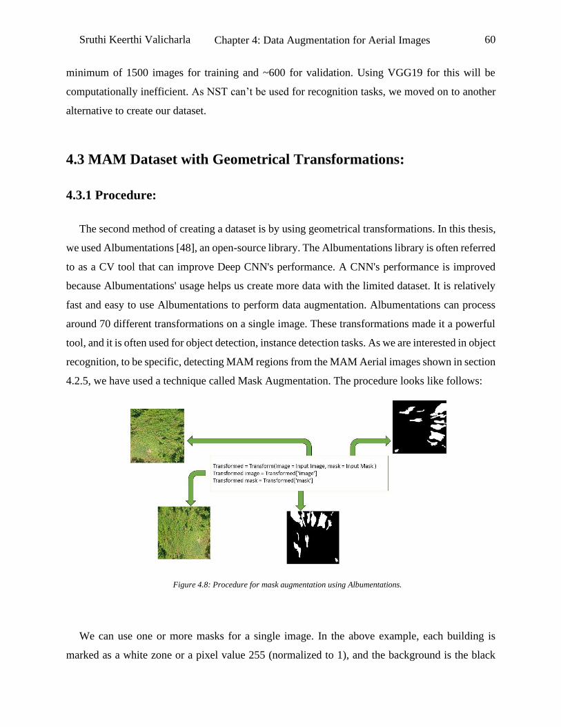
Sruthi Keerthi Valicharla 60
minimum of 1500 images for training and ~600 for validation. Using VGG19 for this will be
computationally inefficient. As NST can’t be used for recognition tasks, we moved on to another
alternative to create our dataset.
4.3 MAM Dataset with Geometrical Transformations:
4.3.1 Procedure:
The second method of creating a dataset is by using geometrical transformations. In this thesis,
we used Albumentations [48], an open-source library. The Albumentations library is often referred
to as a CV tool that can improve Deep CNN's performance. A CNN's performance is improved
because Albumentations' usage helps us create more data with the limited dataset. It is relatively
fast and easy to use Albumentations to perform data augmentation. Albumentations can process
around 70 different transformations on a single image. These transformations made it a powerful
tool, and it is often used for object detection, instance detection tasks. As we are interested in object
recognition, to be specific, detecting MAM regions from the MAM Aerial images shown in section
4.2.5, we have used a technique called Mask Augmentation. The procedure looks like follows:
Figure 4.8: Procedure for mask augmentation using Albumentations.
We can use one or more masks for a single image. In the above example, each building is
marked as a white zone or a pixel value 255 (normalized to 1), and the background is the black
Chapter 4: Data Augmentation for Aerial Images
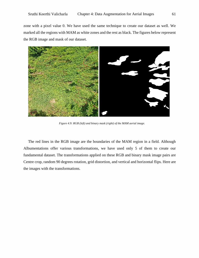
Sruthi Keerthi Valicharla 61
zone with a pixel value 0. We have used the same technique to create our dataset as well. We
marked all the regions with MAM as white zones and the rest as black. The figures below represent
the RGB image and mask of our dataset.
Figure 4.9: RGB (left) and binary mask (right) of the MAM aerial image.
The red lines in the RGB image are the boundaries of the MAM region in a field. Although
Albumentations offer various transformations, we have used only 5 of them to create our
fundamental dataset. The transformations applied on these RGB and binary mask image pairs are
Centre crop, random 90 degrees rotation, grid distortion, and vertical and horizontal flips. Here are
the images with the transformations.
Chapter 4: Data Augmentation for Aerial Images

Sruthi Keerthi Valicharla 62
Transformations Image Mask
Centre crop
Random Rotate 90
Grid Distortion
Chapter 4: Data Augmentation for Aerial Images
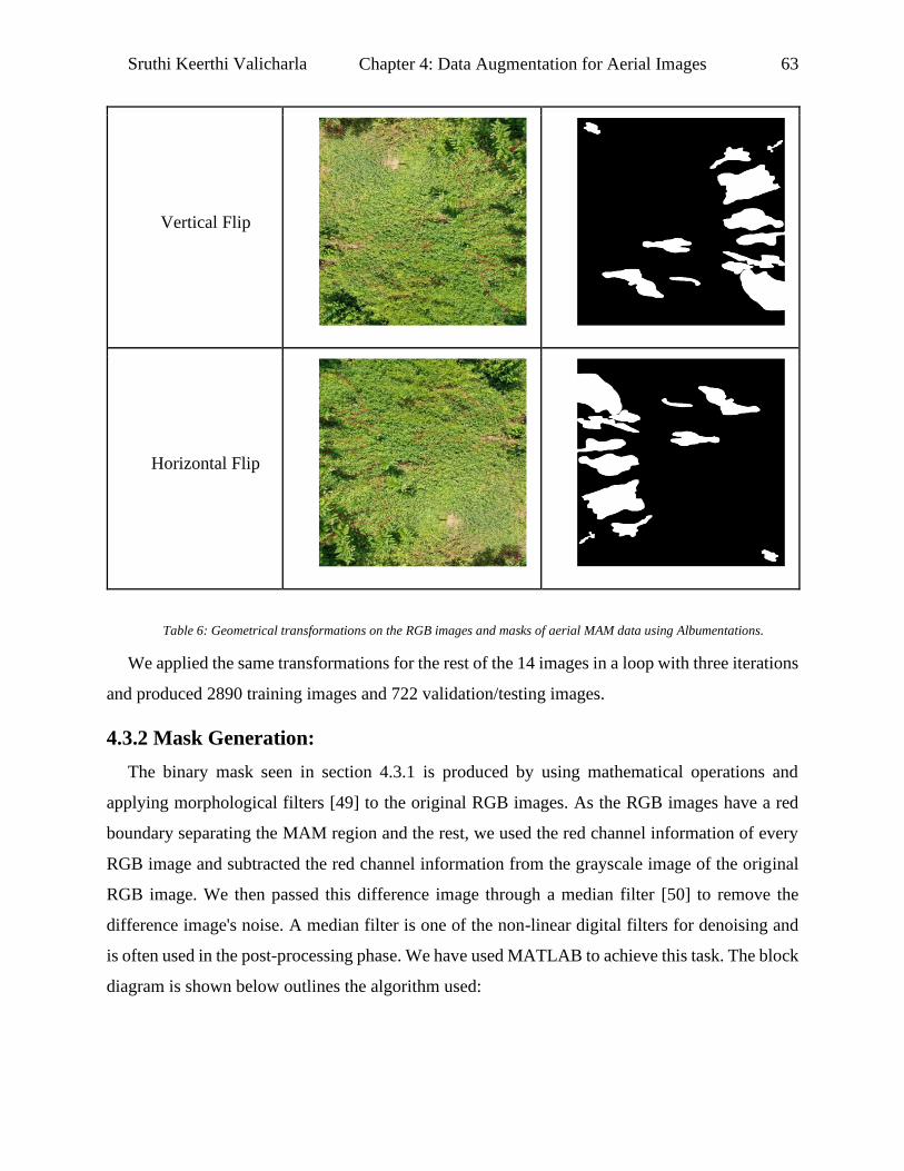
Sruthi Keerthi Valicharla 63
Vertical Flip
Horizontal Flip
Table 6: Geometrical transformations on the RGB images and masks of aerial MAM data using Albumentations.
We applied the same transformations for the rest of the 14 images in a loop with three iterations
and produced 2890 training images and 722 validation/testing images.
4.3.2 Mask Generation:
The binary mask seen in section 4.3.1 is produced by using mathematical operations and
applying morphological filters [49] to the original RGB images. As the RGB images have a red
boundary separating the MAM region and the rest, we used the red channel information of every
RGB image and subtracted the red channel information from the grayscale image of the original
RGB image. We then passed this difference image through a median filter [50] to remove the
difference image's noise. A median filter is one of the non-linear digital filters for denoising and
is often used in the post-processing phase. We have used MATLAB to achieve this task. The block
diagram is shown below outlines the algorithm used:
Chapter 4: Data Augmentation for Aerial Images

Sruthi Keerthi Valicharla 64
Figure 4.10: Block diagram for binary mask generation for the marked aerial RGB images.
Workflow:
1. The input image to the RGB image block to read the image.
2. Extract the red channel information and the grayscale information from the RGB image.
3. Find the difference between red channel and grayscale by using imsubtract.
4. To remove the noise, we applied a 2-D median filter with a 1x1 neighbourhood.
5. We transformed this denoised image into a binary image with a 0.5 level using im2bw.
6. Finally, we used a morphological reconstruction technique to fill the holes using the imfill
function with 18 connectivities.
Figure 4.11: Output of each block. (1) RGB image, (2a) Red channel of the RGB image, (2b) Grayscale of the RGB image, (3)
Difference of 2a and 2b, (4) Difference image after denoising, (5) Binary image of the difference image, (6) Final mask after
morphological reconstruction.
We iterated all the 15 images mentioned in section 4.3.1 to get the masks.
(1) (2a) (2b) (3)
(4) (5) (6)
Chapter 4: Data Augmentation for Aerial Images

Sruthi Keerthi Valicharla 65
4.3.3 Annotations:
As we are using the weights of Mask R-CNN trained on the COCO dataset, we need the
annotations for our dataset to resemble the COCO dataset. As mentioned in section 3.4.2, we used
the COCO standard format for annotation and saved it as a JSON file.
This dataset has only one super category called Weeds and only one object of interest, MAM.
The bounding box values are obtained from the mask generated for each of the augmented images.
With these annotations and the mask details, our dataset looks something like this:
Figure 4.12: Example images from the Augmented MAM dataset.
4.3.4 Limitations:
Our dataset's limitations are that we have considered only 15 real-time drone images for our
data augmentation. Any object detection model will not be able detect the MAM ideally in all
weather and lighting conditions. Also, we have a red boundary around the MAM region in both
training and testing images. The object detection models will most likely search for the red channel
information to get to the MAM region. This drawback can be addressed by removing the human-
made red boundaries from the training and testing dataset. However, the only advantage of having
these red boundaries is that we can better visualize the ground truth and the predicted values for
the people who have no agricultural background.
Chapter 4: Data Augmentation for Aerial Images

Sruthi Keerthi Valicharla 66
Chapter 5:
MAM Detection using Mask R-CNN:
5.1 Introduction:
The scientific name of MAM is Persicaria Perfoliata, formerly known as Polygonum
Perfoliatum. The common names include devil’s tail, Mile-A-Minute, and Asiatic tearthumb. It is
a member of the polygonum family, often referred to as the buckwheat family. MAM falls under
the Eukaryote domain's Plantae kingdom. This plant is native to India and East Asia. However, in
the year 1930, it was accidentally introduced into the USA by contamination of holly seed. Now,
MAM is found in almost all Mid-Atlantic states. MAM usually expands in cool areas because its
seed needs a chilly period of eight weeks to flower. This plant smothers the other plants, trees, and
shrubs by growing on top of them and has a growth rate of 6 inches per day. Because of this
invasive nature, the plants underneath them will not receive enough sunlight for photosynthesis,
and eventually, they become weak. The smothering is caused by the excessive weight and pressure
caused by MAM. Although MAM in the US is only at 20% of its actual potential, it can decline
the vegetation, thereby impacting the wildlife that survives on those plants. The reason for its
potential to destroy the crop plants is that it is an invasive plant, meaning, in a foreign locale, the
invasive plants will not have their natural enemies to stop their growth. The figures below show
the occupancy of MAM in the US.

Sruthi Keerthi Valicharla 67
Figure 5.1: MAM infestation in the US (left) and areas in the east coast infected by MAM (right). Source32
Description of MAM:
MAM is an annual vine with light green leaves. The leaves' dimensions are usually 4-7 cm in
height and 5-9 cm wide. The shape of the leaves is like an equilateral triangle. The vines change
their shades from green to reddish shade, and as it is a vine, it has ocrea that surround the stems.
The flowers are usually white, and the fruits resemble blue berry. MAMs fall under self-fertile
plants as they do not need any pollinators for fertilization. June to October is the prime time in a
year for their fertilization. The seeds that fall on the ground germinate around April through July.
The spread of MAM can be due to these seeds as some birds carry these seeds to long distances.
The birds, animals like squirrels, deer also eat MAM fruits, and their scat may contain MAM seeds.
MAM seeds can float on water for nine days. So, any watershed, storms, or even vines hanging
over water bodies can speed up the spreading of MAM. One more interesting fact about the seeds
of MAM is that they can be viable in the soil for around six years, and they can start germination
anytime. The figures below provide an idea of MAM.
32 http://nyis.info/invasive_species/mile-a-minute/.
Chapter 5: MAM Detection using Mask R-CNN

Sruthi Keerthi Valicharla 68
Figure 5.2: Leaves (left) and fruits (right) of MAM. Source33
The habitat preferred by MAM:
MAM plants are usually found in wet areas, but it is not the only criteria. It can also be seen in
uncultivated farms, roadsides, water stream areas. Although MAM prefers moist soil, it can grow
in dry soil as well. MAM also needs full sunlight. It grows over the top of other plants to reach for
the sunlight. However, it can also grow under partial sunlight.
MAM Management techniques:
Once detected, we need to find a way to eradicate their presence. There are multiple techniques
to do this job. Some of them are:
• Herbicides: Herbicides can be sprayed before the seed germinates or to a growing plant.
The former type is called pre-emergent, and the latter type is called post-emergent.
However, it can be challenging to spray herbicides because the MAM usually grows on top
of a plant, and it is hard to localize the spraying on MAM.
33 http://nyis.info/invasive_species/mile-a-minute/.
Chapter 5: MAM Detection using Mask R-CNN
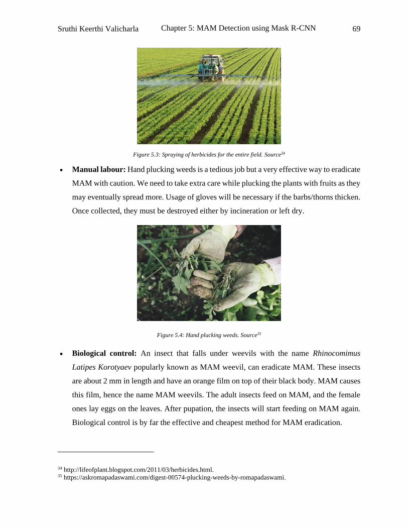
Sruthi Keerthi Valicharla 69
Figure 5.3: Spraying of herbicides for the entire field. Source34
• Manual labour: Hand plucking weeds is a tedious job but a very effective way to eradicate
MAM with caution. We need to take extra care while plucking the plants with fruits as they
may eventually spread more. Usage of gloves will be necessary if the barbs/thorns thicken.
Once collected, they must be destroyed either by incineration or left dry.
Figure 5.4: Hand plucking weeds. Source35
• Biological control: An insect that falls under weevils with the name Rhinocomimus
Latipes Korotyaev popularly known as MAM weevil, can eradicate MAM. These insects
are about 2 mm in length and have an orange film on top of their black body. MAM causes
this film, hence the name MAM weevils. The adult insects feed on MAM, and the female
ones lay eggs on the leaves. After pupation, the insects will start feeding on MAM again.
Biological control is by far the effective and cheapest method for MAM eradication.
34 http://lifeofplant.blogspot.com/2011/03/herbicides.html. 35 https://askromapadaswami.com/digest-00574-plucking-weeds-by-romapadaswami.
Chapter 5: MAM Detection using Mask R-CNN

Sruthi Keerthi Valicharla 70
Figure 5.5: MAM weevil for biological control. Source36
Once the eradication is done, constant monitoring is required because MAM seeds can be viable
for six years in the soil. Constant monitoring will help to reduce further spreading.
Medicinal Values:
Although MAM is notorious for destroying the natural habitat, it is an edible species. The shoots
and tender leaves can be used in cooking as a vegetable or salad. It can be consumed raw as well.
The fruits resemble blue berries, but they taste sweet. Along with these uses, it is used for various
remedies in herbal medicine in China. In Traditional Chinese Medicine (TCM), MAM is often
referred to as gang Bangui (杠板归).
5.2 Three – Level Hierarchy for MAM detection:
To detect MAM using UAVs and avoid false positives, we propose a three-level hierarchy
(forest, trees, and leaves).
Stage 1 - Forest-level survey: The UAVs will be flying at higher altitudes to check for the
agriculture field zones.
Stage 2 - Tree-level survey: Once the agriculture lands were confirmed, the UAVs will drop
to a relatively low altitude, such as 10-15m, as shown in our dataset in section 4.3. We will use
Mask R-CNN to locate the regions with MAM setting the threshold to 85%.
36 http://nyis.info/invasive_species/mile-a-minute/.
Chapter 5: MAM Detection using Mask R-CNN

Sruthi Keerthi Valicharla 71
Stage 3 - Leaf -level survey: After MAM region confirmation, the UAVs will further drop to
5 m to confirm the presence of MAM.
The flow chart is as follows:
Figure 5.6: Flow chart for our three-level hierarchy
Here, the DL block is the Deep Learning block where we use Mask R-CNN for MAM region
prediction. The weed control block can be biological control, herbicides, or manual plucking, as
mentioned in section 5.1
Chapter 5: MAM Detection using Mask R-CNN

Sruthi Keerthi Valicharla 72
5.3 Experiment Setup:
In this section, we focused on the tree level analysis to detect the MAM presence using Mask
R-CNN model. To train the model, we have used the dataset that we have created using the
geometrical transformations in section 4.3. We have generated around 2890 images for training
and 722 images for testing/validation. We have used Resnet 50 FPN as a backbone for feature
extraction. The learning rate used is 0.001, and the number of epochs is 300. The batch size used
is 16, and the number of classes is two as we have MAM as one class and the other being the
background. We used Detectron2 for this experiment because Detectron2 uses a PyTorch frame,
as mentioned in chapter 2, for faster and efficient performance.
5.4 Results and Evaluations:
For testing, we have set two thresholds (0.9, 0.5) for the Softmax. The following images will
provide a detailed understanding of the results with the dataset created in section 4.3.
Figure 5.7: Augmented dataset’s (section 4.3) Mask R-CNN results with Softmax threshold = 0.9. The number on the top of
the bounding box is the probability of MAM’s presence.
In the above results, the red boundaries are our ground truth, and the mask is our prediction.
The network does a pretty good job eliminating unwanted human-made objects such as the helipad,
car, and the human himself. The number on the head of the RoI bounding box is the probability of
Chapter 5: MAM Detection using Mask R-CNN

Sruthi Keerthi Valicharla 73
that segmentation being MAM. Also, we can notice that all of the MAM regions were not detected
on the image on the right because it is not 90% sure to be MAM.
Now, if we set the threshold to 0.5, the network does an OK job identifying those small MAM
patches, but it also detects the other human-made objects as MAM as well with the slightest
probability. The figures below will explain the 0.5 threshold case.
Figure 5.8: Augmented dataset’s (section 4.3) Mask R-CNN results with Softmax threshold = 0.5. With this threshold, we
have false alarms such as car detection.
As we did not specify anything about the car or helipad in our dataset, it is slightly tricky for
the model to eliminate them because the dataset has a red line around the MAM region, and it is
using the red channel information to learn the features of MAM. As the car and the other human-
made objects have shades closer to the MAM red line channel, it could be a miss-hit.
Evaluation:
As our dataset format resembles the COCO dataset and we have used the COCO pre-trained
weights, we have used COCO evaluation metrics to understand our Mask R-CNN's overall
performance. Our model has reached an Average Precision50 [32] of ~98% for the bounding box
prediction and AP50 of ~92%.
Chapter 5: MAM Detection using Mask R-CNN

Sruthi Keerthi Valicharla 74
5.5 Ablation study:
As mentioned in section 3.3, we have used Feature Pyramid Network to serve as our Region
Proposal Network (RPN) block for our Mask R-CNN model. This section will demonstrate why
FPN is a better choice for RPN instead of others by comparing the Average Precision metrics of
standard ResNet-50. We have used ResNet-50-C4 as our other backbone for RPN. Here, C4
represents the 4th stage of the convolutional final convolutional layer.
Backbone AP AP50 AP75 APl
ResNet-50-C4 61.772 87.274 77.221 61.772
ResNet-50-FPN 70.019 98.855 84.895 70.019
Table 7: COCO evaluation metrics for different RPN backbones.
The FPN backbone outperforms the standard ResNet-50-C4 when it comes to precision metrics.
In ResNet-50-C4, we have a single-scale feature extractor at any given level in the RPN block. So,
we need to use multiple anchors at every stage to extract the multi-scale information. These
multiple anchor blocks slower the performance of our model. However, when this single-scale
feature extractor is replaced with an FPN, we will have a single scale assigned to each layer, and
at each level, multiple aspect ratios are used to extract the features. This pyramid architecture of
FPN provides better accuracy and speed compared to the traditional ResNet backbones.
Real-time testing:
Although we have red ground truths in our training dataset, we have tested our model's
performance on an unmarked original image. The results are as follows:
Chapter 5: MAM Detection using Mask R-CNN

Sruthi Keerthi Valicharla 75
Figure 5.9: Mask R-CNN’s performance on real-time data.
Discussion:
The model can still get the MAM region despite having a red boundary (46% bounding box),
but we have a lot of false alarms. To overcome this problem, we would have to remove the red
markings around the RoI in our training image dataset.
Chapter 5: MAM Detection using Mask R-CNN
Sruthi Keerthi Valicharla 76
Chapter 6:
Conclusions and Future Work:
6.1 Conclusions:
In this thesis, we focused on recognition of weed plants in agricultural areas. We have tested
Mask R-CNN’s performance for recognizing plants with two classes and then expanded our
experiment by creating a synthetic data of 80 classes for our field image study. For our aerial image
study, we focused on various methods to create the dataset including localized style transfer and
geometrical transformations. We have tested the performance of Mask R-CNN using this synthetic
aerial image dataset and were able to reach an AP50 of ~91% for the predicted segmentation mask
and ~95% for the predicted bounding box.
6.2 Future Work:
Although we have satisfying results, there are certain limitations to our dataset. We have
considered only one specific lighting condition and background plants as all the images we have
generated using data augmentation technique are from 15 real time images. It can be quite
challenging to recognize the plant species instead of just detecting one specific species. The
following are the proposals for each stage in our hierarchy.

Sruthi Keerthi Valicharla 77
Figure 6.1: Three-level hierarchy. (1) Forest level, (2) Trees level, (3) Plant level.
Proposals:
Stage 1 - Forest-level survey: We need to come up with a good and properly annotated aerial
image dataset to recognize the patterns of agriculture fields that contains MAM.
Stage 2 - Tree-level survey: Although we have a functional Mask R-CNN with decent AP, we
must expand our dataset by considering images with various backgrounds like the plants that
look similar to MAM and also consider various lighting and seasonal conditions.
Figure 6.2: MAM in various lighting conditions.
Stage 3 - Leaf-level survey: We need to train a classifier that can classify MAM versus all the
other common crop and weed plants that resembles MAM. For instance, a vine type called
Microstegium Vimineum or commonly known as Japanese Stilt grass might be similar to
(1) (2) (3)
Chapter 6: Conclusions and Future Work

Sruthi Keerthi Valicharla 78
MAM. But, the challenge of lack of proper dataset persists. We need to collect some images
and apply Super Resolution (SR)37 Techniques to improve the quality of the images collected
from various sources and use those SR images to extract fine features.
Figure 6.3: Weeds similar to MAM: Japanese Stilt grass (left) and Hedge Bindweed (right)
37 A set of techniques to improve the resolution of an image.
Chapter 6: Conclusions and Future Work

Sruthi Keerthi Valicharla 79
Bibliography
[1] Abouziena, H. F., and W. M. Haggag., “Weed control in clean agriculture: a
review1.,” Planta daninha 34.2, pp. 377-392, 2016.
[2] LeCun, Y., Bottou, L., Bengio, Y., & Haffner, P., “Gradient-based learning applied
to document recognition.,” Proceedings of the IEEE, pp. 86(11), 2278-2324, 1998.
[3] Gatys, Leon A., Alexander S. Ecker, and Matthias Bethge., “A neural algorithm of
artistic style.,” arXiv preprint, p. arXiv:1508.06576, 2015.
[4] He, K., Gkioxari, G., Dollár, P., & Girshick, R., “Mask r-cnn,” Proceedings of the
IEEE international conference on computer vision, pp. 2961-2969, 2017.
[5] Haug, Sebastian, and Jörn Ostermann., “A crop/weed field image dataset for the
evaluation of computer vision based precision agriculture tasks.,” European Conference
on Computer Vision. Springer, pp. 105-116, 2014.
[6] Chiu, M. T., Xu, X., Wei, Y., Huang, Z., Schwing, A. G., Brunner, R., ... & Shi, H.,
“Agriculture-vision: A large aerial image database for agricultural pattern analysis.,” In
Proceedings of the IEEE/CVF Conference on Computer Vision and Pattern
Recognition, pp. 2828-2838, 2020.
[7] Simonyan, Karen, and Andrew Zisserman., “Very deep convolutional networks for
large-scale image recognition.,” arXiv preprint arXiv:1409.1556, 2014.
[8] Mallah, C., Cope, J., & Orwell, J. , “Plant Leaf Classification using Probabilistic
Integration of Shape, Texture and Margin Features.,” Pattern Recognit. Appl., 3842.,
2013.
[9] Huang, Mei-Ling; Chang, Ya-Han, “Dataset of Tomato Leaves,” Mendeley Data, V1,
doi: 10.17632/ngdgg79rzb.1, 2020.
[10] CHOUHAN, Siddharth Singh; Kaul, Ajay; SINGH, UDAY PRATAP; & Science,
Madhav Institute of Technology , “ A Database of Leaf Images: Practice towards Plant
Sruthi Keerthi Valicharla 80
Conservation with Plant Pathology,,” Mendeley Data, V4, doi: 10.17632/hb74ynkjcn.4,
2020.
[11] Mohanty, S. P., Hughes, D. P., & Salathé, M, “Using deep learning for image-based
plant disease detection.,” Frontiers in plant science, 7, 1419, 2016.
[12] Olsen, A., Konovalov, D. A., Philippa, B., Ridd, P., Wood, J. C., Johns, J., ... &
White, R. D. , “DeepWeeds: A multiclass weed species image dataset for deep
learning.,” Scientific reports, 9(1), 1-12., 2019.
[13] Lameski, Petre & Zdravevski, Eftim & Trajkovik, Vladimir & Kulakov, Andrea. ,
“Weed Detection Dataset with RGB Images Taken Under Variable Light Conditions.,”
112-119. 10.1007/978-3-319-67597-8_11. , 2017.
[14] Minervini, M., Fischbach, A., Scharr, H., & Tsaftaris, S. A. , “Finely-grained
annotated datasets for image-based plant phenotyping.,” Pattern recognition letters, 81,
80-89., 2016.
[15] Giselsson, T., Dyrmann, M., J\orgensen, R., Jensen, P., & Midtiby, H., “ A Public
Image Database for Benchmark of Plant Seedling Classification Algorithms.,” arXiv
preprint., 2017.
[16] Sudars, K., Jasko, J., Namatevs, I., Ozola, L., & Badaukis, N. , “Dataset of annotated
food crops and weed images for robotic computer vision control.,” Data in brief, 31,
105833. https://doi.org/10.1016/j.dib.2020.105833, 2020.
[17] Wang, A., Zhang, W., & Wei, X. , “A review on weed detection using ground-based
machine vision and image processing techniques.,” Computers and electronics in
agriculture, Vols. 158, 226-240, 2019.
[18] Bakhshipour, A., & Jafari, A. , “ Evaluation of support vector machine and artificial
neural networks in weed detection using shape features,” Computers and Electronics in
Agriculture, Vols. 145, 153-160, 2018.

Sruthi Keerthi Valicharla 81
[19] Yu, J., Sharpe, S. M., Schumann, A. W., & Boyd, N. S. , “Deep learning for image-
based weed detection in turfgrass.,” European journal of agronomy, Vols. 104, 78-84,
2019.
[20] Yu, J., Schumann, A. W., Cao, Z., Sharpe, S. M., & Boyd, N. S. , “ Weed detection
in perennial ryegrass with deep learning convolutional neural network.,” frontiers in
Plant Science, no. 10, 1422, 2019.
[21] dos Santos Ferreira, A., Freitas, D. M., da Silva, G. G., Pistori, H., & Folhes, M. T. ,
“Weed detection in soybean crops using ConvNets,” Computers and Electronics in
Agriculture, Vols. 143, 314-324, 2017.
[22] Louargant, M., Jones, G., Faroux, R., Paoli, J. N., Maillot, T., Gée, C., & Villette, S. ,
“Unsupervised classification algorithm for early weed detection in row-crops by
combining spatial and spectral information,” Remote Sensing, no. 10(5), 761, 2018.
[23] Bah, M. D., Hafiane, A., & Canals, R. , “Deep learning with unsupervised data
labeling for weed detection in line crops in UAV images.,” Remote sensing, 10(11),
1690., 2018.
[24] Hertzmann, A., Jacobs, C. E., Oliver, N., Curless, B., & Salesin, D. H. , “Image
analogies,” In Proceedings of the 28th annual conference on Computer graphics and
interactive techniques , pp. 327-340, 2001.
[25] Efros, Alexei A., and William T. Freeman., “Image quilting for texture synthesis and
transfer.,” Proceedings of the 28th annual conference on Computer graphics and
interactive techniques., 2001.
[26] Jetchev, N., Bergmann, U., & Vollgraf, R., “Texture Synthesis with Spatial
Generative Adversarial Networks.,” arXiv preprint arXiv:1611.08207, 2016.
[27] Bergmann, U., Jetchev, N., & Vollgraf, R. , “Learning Texture Manifolds with the
Periodic Spatial GAN.,” arXiv preprint arXiv:1705.06566, 2017.

Sruthi Keerthi Valicharla 82
[28] A. J. W. a. M. X. Wells, “Localized Style Transfer”.
[29] Gatys, L. A., Bethge, M., Hertzmann, A., & Shechtman, E, “Preserving color in
neural artistic style transfer,” arXiv preprint arXiv:1606.05897, 2016.
[30] Zheng, X., Chalasani, T., Ghosal, K., Lutz, S., & Smolic, A. , “Stada: Style transfer
as data augmentation.,” arXiv preprint arXiv:1909.01056., 2019.
[31] Howard, Andrew G., Menglong Zhu, Bo Chen, Dmitry Kalenichenko, Weijun Wang,
Tobias Weyand, Marco Andreetto, and Hartwig Adam., “Mobilenets: Efficient
convolutional neural networks for mobile vision applications.,” arXiv preprint
arXiv:1704.04861, 2017.
[32] Lin, T. Y., Maire, M., Belongie, S., Hays, J., Perona, P., Ramanan, D., ... & Zitnick,
C. L., “Microsoft coco: Common objects in context.,” European conference on
computer vision. Springer, Cham, pp. 740-755, 2014.
[33] Ren, S., He, K., Girshick, R., & Sun, J. , “Faster R-CNN: towards real-time object
detection with region proposal networks.,” IEEE transactions on pattern analysis and
machine intelligence, 39(6), 1137-1149., 2016.
[34] Lin, T. Y., Goyal, P., Girshick, R., He, K., & Dollár, P., “Focal loss for dense object
detection.,” In Proceedings of the IEEE international conference on computer vision,
pp. 2980-2988, 2017.
[35] Cai, Z., & Vasconcelos, N., “Cascade r-cnn: Delving into high quality object
detection.,” In Proceedings of the IEEE conference on computer vision and pattern
recognition, pp. 6154-6162, 2018.
[36] Kirillov, A., Girshick, R., He, K., & Dollár, P. , “Panoptic Feature Pyramid
Networks,” In Proceedings of the IEEE/CVF Conference on Computer Vision and
Pattern Recognition , pp. 6399-6408, 2019.

Sruthi Keerthi Valicharla 83
[37] S. Hochreiter, “The vanishing gradient problem during learning recurrent neural nets
and problem solutions.,” International Journal of Uncertainty, Fuzziness and
Knowledge-Based Systems, 6(02), 107-116., 1998.
[38] Girshick, R., Donahue, J., Darrell, T., & Malik, J. , “Rich feature hierarchies for
accurate object detection and semantic segmentation.,” In Proceedings of the IEEE
conference on computer vision and pattern recognition , pp. 580-587, 2014.
[39] Felzenszwalb, P. F., & Huttenlocher, D. P., “Efficient graph-based image
segmentation,” International journal of computer vision 59(2) , 167-181, 2004.
[40] R. Girshick, “Fast r-cnn,” Proceedings of the IEEE international conference on
computer vision., 2015.
[41] Ren, S., He, K., Girshick, R., & Sun, J., “Faster r-cnn: Towards real-time object
detection with region proposal networks.,” arXiv preprint arXiv:1506.01497., 2015.
[42] Lin, T. Y., Dollár, P., Girshick, R., He, K., Hariharan, B., & Belongie, S., “Feature
Pyramid Networks for Object Detection,” In Proceedings of the IEEE conference on
computer vision and pattern recognition, pp. 2117-2125, 2017.
[43] He, K., Zhang, X., Ren, S., & Sun, J. , “Deep Residual Learning for Image
Recognition,” In Proceedings of the IEEE conference on computer vision and pattern
recognition, pp. 770-778, 2016.
[44] Roy, P., Ghosh, S., Bhattacharya, S., & Pal, U., “Effects of Degradations on Deep
Neural Network,” arXiv preprint arXiv:1807.10108., 2018.
[45] Gatys, L. A., Ecker, A. S., & Bethge, M., “Image style transfer using convolutional
neural networks.,” In Proceedings of the IEEE conference on computer vision and
pattern recognition , pp. 2414-2423, 2016.

Sruthi Keerthi Valicharla 84
[46] Deng, J., Dong, W., Socher, R., Li, L. J., Li, K., & Fei-Fei, L., “Imagenet: A large-
scale hierarchical image database,” In 2009 IEEE conference on computer vision and
pattern recognition, pp. 248-255.
[47] Champandard, Alex J., “Semantic style transfer and turning two-bit doodles into fine
artworks.,” arXiv preprint arXiv:1603.01768 , 2016.
[48] A. Buslaev, V., & A.~A. Kalinin , “Albumentations: fast and flexible image
augmentations.,” ArXiv e-prints, 2018.
[49] Serra, J., & Vincent, L. , “An overview of morphological filtering.,” Circuits,
Systems and Signal Processing, 11(1), 47-108., 1992.
[50] Arce, G. R., Gallagher, N. C., & Nodes, T. A., “Median filters: theory for one-and
two-dimensional filters.,” Advances in computer vision and image processing, 2, 89-
166., 1986.
[51] Zheng, Yufeng & Yang, Clifford & Merkulov, Aleksey. , “Breast cancer screening
using convolutional neural network and follow-up digital mammography.,” 4.
10.1117/12.2304564., 2018.
![Transferability of the Deep Learning Mask R-CNN Model for ......AsecondWorldView-2image(imageID:10300100468D9100,7July2015,withanx-andy-resolution of 0.48 0.49 m, Imagery ' [2015]](https://img.dokumen.tips/doc/110x75/60b6141f63ebe15b3d7af9f2/transferability-of-the-deep-learning-mask-r-cnn-model-for-asecondworldview-2imageimageid10300100468d91007july2015withanx-andy-resolution.jpg)


![arXiv:1809.08545v3 [cs.CV] 16 Apr 2019 · 3.1. Bounding Box Parameterization Based on a two-stage object detector Faster R-CNN or Mask R-CNN [42,17] shown in Figure3, we propose to](https://img.dokumen.tips/doc/110x75/5f0e99687e708231d44003ae/arxiv180908545v3-cscv-16-apr-2019-31-bounding-box-parameterization-based.jpg)


![TensorMask: A Foundation for Dense Object Segmentation · rate predictions, as pioneered by Faster R-CNN [34] and Mask R-CNN [17] for bounding-box object detection and instance segmentation,](https://img.dokumen.tips/doc/110x75/5e386a20c7754528ff72ed34/tensormask-a-foundation-for-dense-object-segmentation-rate-predictions-as-pioneered.jpg)


![cs230.stanford.educs230.stanford.edu/files_winter_2018/projects/6937153.pdf · 3.3.2 Mask RCNN Mask R-CNN is an extension of the Faster RCNN model [2]. Faster R-CNN is a Region Proposal](https://img.dokumen.tips/doc/110x75/5e448090b525a912e76a06e0/cs230-332-mask-rcnn-mask-r-cnn-is-an-extension-of-the-faster-rcnn-model-2.jpg)