Embed Size (px)
Citation preview

Webs, mandibles and capsules - Is
mapped vegetation type a surrogate for
beetle and spider assemblages?
by
Lynette G. Forster BA.
(University of Tasmania)
A thesis submitted in partial fulfilment of the requirements for a
Masters Degree in Environmental Management at the School of
Geography and Environmental Studies, University of Tasmania
June 2007
ii
Declaration
This thesis contains no material which has been accepted for the award
of any other degree or diploma in any tertiary institution, and to the best
of my knowledge and belief, contains no material previously published
or written by another person, except where due reference is made in the
text of the thesis.
Signed
Lynette Forster BA
During the process of reducing memory and conversion to pdf in order to make
this thesis available electronically on the web, some formatting errors occurred,
particularly in the results chapter. Apologies.

iii
Abstract
Increasingly, the effectiveness of surrogate species as a management tool for
reservation of biodiversity has been questioned. It has been established that mammal
and bird distributions correspond to vegetation type, but for invertebrate species this
is less clear. This assumption was tested by comparing the communities of species of
two invertebrate taxa in forest litter, spiders and beetles with pitfall sampling.
Sampling occurred in spring summer and autumn in the foothills of Mount Wellington
in 2002 and 2003 within 6 different adjacent eucalypt forest types - Eucalyptus
regnans forest (WRE), E. obliqua with broadleaf shrubs (WOB), E. obliqua dry forest
(DOB), E. tenuiramis forest on sediments (DTE), E. amygdalina forest on mudstone
(DAM) and E. pulchella forest (DPU).
The total number of beetles collected was 1726, representing 152 species from 28
families. Spiders totalled 1983 representing 204 species from 20 families. A third of
these were juveniles and data were analysed separately with and without the juveniles.
Forest type was a significant factor affecting distribution of spiders and beetles but
was different for different forest types.
There was a significantly different spider community in wet WOB while communities
in WRE and dry DOB overlapped suggesting change along a continuum from wet to
dry forest. Species responsible were vagrant hunters from the families Corrinidae,
Gnaphosidae, Lycosidae, Zodariidae, Zoridae and a Micropholcommatidae web
builder. Beetles were also significantly different between dry E. tenuiramis (DTO)
and E. amygdalina (DAM) and a wet WRE-WOB-DOB continuum was detected.
Species responsible for this separation were Isopteron obscurum (Erichson, 1842):
Tenebrionidae, Tetrabothrus claviger (Fauvel, 1878): Staphylinidae and some
fungivores - Nemadini (Leiodidae), Scaphidium sp.: Staphylinidae, Thalycrodes
australe (Germar, 1848): Nitidulae, and Acrotrichis sp.: Ptilidae.

iv
A total of 56 soil, topographic, ground cover, microclimate and vegetation variables
were measured. Their significance for predicting the distributions of spiders and
beetles better than vegetation alone was examined. Statistical analysis revealed
environmental gradients along which beetles and spiders were dispersed. Beetles were
distributed along a moisture and a ground cover gradient. Spiders were separated
along a soil nutrient and a moisture/temperature gradient. These gradients varied
among sites in the same forest type as well as among sites in different forest types,
and explained some of the site scale variation in assemblages.
At a larger geographic scale, sampling at 36 sites grouped into 3 regions in
southeastern Tasmania: Hobart, Levendale and Swansea, tested assemblage
differences across a span of 157 km. Beta diversity was highest at the scale of 50 km.
This is suggested as the maximum distance that should separate patches of the same
forest type in order to capture maximum spatial variation in diversity of beetles and
spiders across a vegetation based reserve mosaic. The research highlights the
complexity of invertebrate interactions with forest type and environmental variables
and indicates that simple prescriptions which can inform planning of reserves are not
readily obtainable from examination of assemblages as a whole.
Theridiidae Segestriidae Zodariidae Zodariidae

v
Acknowledgments
Thanks to my Supervisor, Dr Peter McQuillan, whose depth of knowledge about
invertebrates was invaluable. I am grateful to Dr Simon Grove and Belinda Yaxley for
access to the Tasmanian Forestry Insect Collection to aid with identification, to Liz
Turner for access to the Tasmanian Museum spider collection and Lisa Boutin and
Beck Harris for assistance with spider identification. Dr Cathy Young provided access
to the DPI beetle collection and willingly shared her immense expertise.
Particular thanks to Dr Nicky Meeson for acquainting me with her study sites and
making the beetle and spider by-catch from her ant research available to me and
offering a multitude of other support.
Thanks to Kristin Pedderson, Derek Harnwell and Robyn Gottschalk for field work
assistance. Their preliminary separation of beetles and spiders was invaluable and in
Robyn’s case her contribution was admirable considering her arachnophobia!
Thanks to the CRC Ecology Discussion Group for in depth discussions on statistical
analysis, research methodology, and the lives of beetles, particularly Dr Sue Baker, Dr
Marie Yee and Dr Anna Hopkins.
Thanks to support staff in the Department of Geography and Environmental Studies -
David Sommerville for equipment such as digital cameras, Darren Turner for his
ingenious programme which converted digital photos into percentage of canopy cover
and Dennis Charlesworth for technical equipment and for undertaking an enormous
part of the rather onerous, (but worthwhile) soil analysis.
I specially thank Sapphire McMullan-Fisher who inspired my journey into
investigation of the ecological world, imparted endless knowledge of fungi and
identified some of my collection
Finally, a big thankyou to my children Owen, Amy, Huw and Rachel for their
patience and through whose eyes I became acquainted with beetles and spiders, to
Jason the computer wiz who rescued documents and Emma for her delicious
mulligatawny soup.

vi
Preface
Table of Contents
Declaration ………………………………………………………………………..ii
Abstract ………………………………………………………………………..iii
Acknowledgments ………………………………………………………………...v
Preface ……………………………………………………………………………vi
Table of Contents ………………………………………………………………..vi
Introduction …………………………………………………………………………1
Policy context of biological diversity: global to local …………………………1
RESEARCH QUESTION: …………………………………………………………6
RESEARCH OBJECTIVES …………………………………………………………6
Thesis Outline …………………………………………………………………………7
Chapter 1 Background …………………………………………………………8
1.1 Species diversity as a measure of biodiversity …………………………8
1.2 The adequacy of vegetation type as a surrogate for biodiversity reservation….9
Chapter 2 Material and Methods ………………………………………………..20
2.1 Study sites ………………………………………………………………..20
2.2 Sampling of spiders and beetles ………………………………………..27
Biophysical attributes ………………………………………………………………..29
2.3 Statistical analysis ……………………………………………………….37
Chapter 3 Results ……………………………………………………………….51
3.1 Abiotic variables ……………………………………………………… 51
3.2 Plant species ………………………………………………………………59

vii
3.3 Beetle Assemblages …………………………………………………….59
3.4 Spider assemblages …………………………………………………….68
3.5 Statistical Analysis of data …………………………………………… 74
Chapter 4 Discussion …………………………………………………..115
Chapter 5 Implications and Conclusion …………………………………..131
References …………………………………………………………………..134
Sydnesus cornutus (Fabricius, 1801)
Lucanidae

viii
List of Tables
Table 2.1 Forest types sampled in the study ………………………………..24
Table 2.2 Braun-Blanquet score for vegetation cover ………………………..36
Table 2.3 Partial variation: environmental variables X1 and spatial variables
X2…………………………………………………………………………….............49
Table 3.1 Mean canopy cover in each forest type…………………………….…. .52
Table 3.2 Volume of coarse woody debris > 5m diameter ……………………54
Table 3.3 Average volume of fungi in each forest type and standard error …...55
Table 3.4 Summary mean soil nutrients ………………………………………..57
Table 3.5 List of the most abundant beetle species, Mt Wellington foothill sites
……………………………………………………………………………….60
Table 3.6 Ranked abundance of beetle families and number of species ……….60
Table 3.7 Mean abundance and species richness of beetles by trophic guild …67
Table 3.8 Ranked order of abundance of spider families, and species
richness……………………………………………………………………………..69
Table 3.9 Ranked abundance of spider species, abund > 4, Mt Wellington …..70
Table 3.10 Whittaker’s B-diversity index, Mt Wellington species……………..75
Table 3.11 Table of Whittaker’s B-diversity index, regional species …….........77
Table 3.12 Results of one-way anovas for species occurrences in forest types. 78
Table 3.13 Pairwise a posteriori comparisons of dissimilarity between forest
type.............................................................................................................................78
Table 3.14 Permutational Test of Multivariate Dispersion ………………79

ix
Table 3.15 Pair-wise a posteriori comparisons of beetles among forest types. .80
Table 3.16 Average within group dissimilarity for beetles and spiders ………..81
Table 3.17 Matrices of Bray-Curtis dissimilarities within & between groups…81
Table 3.18 Summary CAP results to determine the effect of forest type ………..88
Table 3.19 Highest correlation values of canonical axes with original axes, CAP
………………………………………………………………………………..89
Table 3.20 Correlation of canonical axes with original axes from CAP analyses of
environmental variables. ……………………………………………………..…91
Table 3.21 Subsets of environmental variables and vegetation species that shared
the nearest dissimilarity rank correlation with species dissimilarity ranks…....99
Table 3.22 Fractions of variation partitioned by three sets of variables ………103
Table 3.23 Potential indicator beetle species for different forest types. ………107
Table 3.24 Potential indicator spider species. ……………………………...107
Table 3.25 Results of permutational NPMANOVA……………………………..108
Table 3.26 Results of pair-wise a posteriori comparisons for permutational non-
parametric multivariate analysis of variance. ……………………………...109
Table 4.1 Species whose distribution was correlated with forest type, CAP….119
Table 4.2 Variation in beta diversity measured at different scales…………….127
List of Figures
Figure 0.1 Map of Tasmania’s nine IBRA bioregions. ………………………..3
Figure 2.1 Location of Intensive study sites in the foothills of Mount Wellington
……………………………………………………………………………….21

x
Figure 2.2 Location of Extensive study sites (Hobart, Levendale and Swansea)
……………………………………………………………………………….22
Figure 2.3 Distribution of the six forest types sampled by this research ……….23
Figure 2.4 Site photos representing the variation between forest types………..26
Figure 2.5 Pitfall trap design used in sampling ……………………………….27
Figure 2.6 Sample photo of the canopy taken from ground level ……………….31
Figure 2.7 Diagram of partitioned variation of species assemblages…………...49
Figure 3.1 Regional variation in altitude of sites ……………………………….51
Figure 3.2 Range of aspect orientation of sites in the Mt Wellington foothills. 51
Figure 3.3 Mean canopy cover in each forest type………………………………52
Figure 3.4 Summer and winter solar radiation at each site ……………...53
Figure 3.5 Variation of CWD (Coarse Woody Debris) and its hardness……..54
Figure 3.6 Volume of fungi at each site grouped by forest type …………….56
Figure 3.7 Average volume of fungi in each forest type …………………….56
Figure 3.8 Average topsoil nutrients for each vegetation type …………….58
Figure 3.9 Average subsoil nutrients for each vegetation type …………….59
Figure 3.10 Beetle family richness at Mt Wellington sites …………….61
Figure 3.11 Graphs of mean abundance of common beetles forest types……63
Figure 3.12 Seasonal abundance of beetles in different forest types, Mt
Wellington …………………………………………………………………….64
Figure 3.13 Seasonal occurrence of some Mt Wellington beetles …………….66
Figure 3.14 Mean abundance of beetle species grouped by trophic level……67

xi
Figure 3.15 Graphed rank abundance of adult spider families ……………...69
Figure 3.16 Graph of ranked abundance of the dominant 35 spider families....71
Figure 3.17 Seasonal abundance and species richness of spiders by forest type.
……………………………………………………………………………....72
Figure 3.18 Seasonal abundance of some spiders in different forest types…….73
Figure 3.19 Mean abundance species richness of web builders and vagrant
hunters ……………………………………………………………………….74
Figure 3.20 Comparison of beetle and spider abundance and species richness...75
Figure 3.21 Ordinations of sites in different species spaces. ………………..84
Figure 3.22 Boxplots of mean ranks of dissimilarity for the effect of forest type
………………………………………………………………………………..87
Figure 3.23 Canonical correlation axes plotted for beetle species …….…90
Figure 3.24 Plots of two PCA and canonical axes from CAP analysis for
beetles…………………………………………………………………………….…92
Figure 3.25 NMDS ordination of sites in species space ……………………....93
Figure 3.26 Beetle variation explained by PCA (CCA with environmental data)
……………………………………………………………………………...94
Figure 3.27 Regression trees for site regressed against environmental variables
…………………………………………………………………………...…..96
Figure 3.28 Plots of distances site pairs vs species dissmilarity ………….......101
Figure 3.29 Diagrams of partitioned variation as fractions of species variation.
………………………………………………………………………………………103
Figure 3.30 NMDS plots of sites grouped in species space with species biplots 105

xii
Figure 3.31 NMDS Ordination of regional sites in species space ……………..110
Figure 3.32 NMDS Ordination of regional sites in species space ………………111
Figure 3.33 Mantel test: Plots of site distances against species dissimilarity 112
Figure 3.34 The effect of region and forest type on species communities. Boxplots
of mean ranks dissimilarity ranks between and within groups. ………………113
Figure 4.1 Diagram of forest types from a posteriori NP-MANOVA comparisons
of dissimilarity between beetle assemblages in mapped forest types…………..116
Figure 4.2 Diagram of forest types from a posteriori NP-MANOVA comparisons
of dissimilarity between spider assemblages in mapped forest types………….117
Figure 4.3 Diagram of beetle distributions from canonical
correlation………………………………………………………………………….120
Figure 4.4 Diagram of environmental gradients identified as associated with
beetle and spider assemblages…………………………………………………….121

13

_________________________________________________ Introduction
1
Introduction
Policy context of biological diversity: global to local
Arising from the Earth Summit in Rio de Janeiro in 1992 Australia ratified the
Convention on Biological Diversity in 1993 (Commonwealth of Australia, 1995) and
committed itself to conservation of biological diversity. Soon after, Australia became
part of the Montreal Process which is a working group that establishes and
implements a framework of criteria and indicators for assessing sustainable
management and conservation of temperate and boreal forests. It was formed in 1994
and membership countries cover 90% of the world’s temperate and boreal forests
(Montreal Process Working Group, 1995). The indicators were endorsed as voluntary
guidelines for policy makers under the Santiago Declaration in the ten member
countries - Australia, Canada, Chile, China, Japan, Republic of Korea, Mexico, New
Zealand, Russian Federation and United States of America.
Biological diversity is one of seven criteria in the Montreal Process and three
components have been identified for its assessment: ecosystem, species and genetic
diversity. Species diversity, which is measured by the number of forest dependent
species and their reservation status (Montreal Process Working Group 1995), has
largely focused on plant species; and ecosystem diversity has been characterised by
forest type (Montreal Process Working Group, 1995). Thus vegetation type and
diversity have become default measures of diversity due to lack of extensive,
comprehensive surveys of other taxa. In Tasmania recent research (Baker 2006; Baker
et al. 2007; Grove and Yaxley 2005; Michaels and McQuillan 1995) has contributed
to a body of knowledge about forest dependent beetles which are becoming
identifiable as indicator species that could be incorporated into biological diversity
assessments in the State.
The National Strategy for Ecologically Sustainable Development (Commonwealth of

_________________________________________________ Introduction
2
Australia, 1992) arose from international obligations under Agenda 21 (UNCED,
1992) and provides directions for Australian policy making to conserve biological
diversity as one component of ecologically sustainable development. Progress in
ecologically sustainable development is reported through State of the Environment
Reporting where there have been efforts to identify suites of biologically and
ecologically representative and sensitive taxa to which a pressure/condition/response
model can be applied for planning (Saunders et al. 1998).
Commonwealth protection of biodiversity is now facilitated through the National
Strategy for the Conservation of Australia’s Biological Diversity (Department of
Environment, Sports and Territories 1996). The strategy’s objectives include
identification of ecosystems and threatening processes, species and subspecific
variation, bioregional planning and management, conservation management,
establishment of a comprehensive, adequate and representative system of protected
areas (the CAR system), improving biological diversity conservation outside reserves,
and recognition of the ethnobiological knowledge of indigenous people. Within this
framework the Interim Biogeographic Regionalisation for Australia (IBRA)
(Environment Australia, 2000) provides a landscape-based approach to mapping
ecosystems across Australia resulting in biotic and abiotic information for
conservation of biodiversity instead of solely vegetation data.
Bioregions (Figure 0.1) are based on mapped environmental attributes rather than raw
data, since these attributes are reflected by flora and fauna patterns of distribution
(Thackway and Cresswell 1995). In Tasmania regions are grouped by their similarity
in landform, geology/lithology, climate, vegetation and floristics (Environment
Australia 2000) and build upon Orchard’s 13 biogeographical regions (including
Macquarie Island) for herbarium records (Orchard, 1988), in use since 1982. In the
mid 1980s the Tasmanian Forestry Commission modified the Hebarium regions
slightly and adopted 11 Nature Conservation Regions (including Macquarie Island) by
removing Mt Field and Mt Wellington as separate regions (Orchard 1988).

_________________________________________________ Introduction
3
As reports by the IBRA point out (Thackway and Cresswell 1995), IBRA provides a
guide for identifying gaps in our National reserve system, but is not a basis for
reservation of particular land parcels. The IBRA can assist planning to fill gaps in the
reserve system based on comprehensiveness and representativeness but does not assist
with the third CAR criteria of adequacy, a criteria which needs to be explored at a
finer scale and should include variables outside the scope of the IBRA such as the
level of threat to biodiversity (Thackway and Cresswell 1995). Comprehensiveness is
the degree to which the full range of ecological communities and their biological
diversity are incorporated in the reserve system (RPDC 2003).
Figure 0.1 Map of Tasmanian Interim Biogeographic Regionalisation for Australia (IBRA
Regions) displaying Tasmania’s nine bioregions. The map is based on information from
http://www.deh.gov.au/parks/nrs/ibra/version5-1/tas.html
In Tasmania conservation of biodiversity is managed by reserving different vegetation
types. The underlying assumption that the distribution of other species follows that of
vegetation type (Panzer and Schwartz 1998; Scott et al. 1993) has been questioned

_________________________________________________ Introduction
4
(Ferrier et al. 1999; Mesibov 1993; Oliver et al. 1998; York 1999). Vegetation type is
a commonly selected surrogate for all biodiversity because it is relatively easy to map
from aerial photos compared with comprehensive on-ground surveys of the
distribution of a variety of vertebrate and invertebrate species in several taxa.
Under the 1997 Tasmanian RFA (Regional Forestry Agreement) biodiversity is
reserved through reservation of representative vegetation types of which 50 different
types have been mapped (Harris and Kitchener 2005).
While several studies show that the distribution of mammals and birds have
distribution patterns which follow vegetation types (French, 1999), the same is not
true for invertebrates such as carabid beetles (Michaels 1999), and a study in
Tasmanian rainforests demonstrated that a distinct invertebrate rainforest fauna was
not identifiable (Mesibov 1993). Studies in other parts of Australia have also found
poor congruence between invertebrate assemblages and forest types (Oliver et al.
1998) or remnant size (Major et al. 1999; Gibb and Hochuli 2002). Assemblages in
small fragments of a forest type are not a subset of species found in larger fragments,
being instead, entirely different (Major et al. 1999; Gibb and Hochuli,\ 2002) or
intermediate between continuous native vegetation and wildlife strips (Grove and
Yaxley 2005); again indicating that vegetation type is not the primary factor
influencing invertebrate assemblages (Coy et al. 1993). Hypothetical reserves based
on surrogate species have been found to be no more effective in protecting overall
species richness than reserves based upon a random suite of species (Andelman and
Fagan 2000). It has been demonstrated that selection of the largest patches of habitat
can perform almost as well as a data-intensive search for indicator species (Podani et
al. 1997); while Araujo et al. (2001), found that the representation of species by
environmental diversity was not significantly different from the level obtained by
selecting the same number of areas randomly. ‘Given the numerical dominance of
invertebrates, it is not surprising that the efficacy of basing acquisition decisions
primarily on plant criteria is being questioned,’(Panzer and Schwartz 1998, p. 694).
The influence on invertebrates of many factors including litter depth (Michaels and
McQuillan 1995; York 1999), disturbance history (Mossakowski et al. 1990),
geographical distance (Oliver et al. 1998), microclimate, organic matter and physical

_________________________________________________ Introduction
5
and geographical features (Ferreira and Silva 2001) have been recognised and
considered to be better predictors of invertebrate abundance than vegetation type
(Mesibov 1993). Others have demonstrated that invertebrates do not respond to forest
type but variation in the structure of vegetation (Coy et al. 1993; Greenslade and New
1991; York 1999), biochemical properties of plants and genetic variation within plant
species (Bangert et al. 2006; Dungey et al. 2000). For this reason a large number of
environmental variables have been measured during this research to identify variables
that might provide better surrogate measures for invertebrates.
The research is significant because reservation of biodiversity in Tasmania is largely
based on vegetation type since it is easier to map yet it is not known to what extent
vegetation as a surrogate adequately reserves invertebrate diversity. To do this, spider
and beetle assemblages were not only examined at a small scale in an intensive study
at a local set of adjacent sites, but were compared at a larger scale at three locations
(Hobart, Levendale and Swansea) within the bioregion of Eastern Tasmania.
Knowledge about invertebrates gained from this study will contribute to use of
invertebrates to monitor the health of different vegetation types for the protection of
biodiversity which is threatened by human impacts. Invertebrates respond quickly to
changes in their environment and are increasingly being used as indicators of impacts
on ecosystems of permissable human activities such as grazing and fire (Harris et al.
2003), firewood collection (ANZECC 2001), timber harvesting (Baker et al. 2007)
and silviculture (Michaels and McQuillan 1995) within, or adjacent to, reserved
vegetation types. Invertebrate monitoring can provide a valuable tool for monitoring
sustainable management and protection of Tasmania’s variety of vegetation types. It
is also expected that the results of this study may contribute to refining an appropriate
suite of surrogate species which could be representative of invertebrate biodiversity in
Tasmania and contribute to the debate on the effectiveness of surrogacy in
conservation management.

_________________________________________________ Introduction
6
RESEARCH QUESTION:
The broader scope of this thesis addresses the topical question whether vegetation
type is an appropriate surrogate for invertebrate biodiversity. My specific test of this
question focuses on two biodiverse invertebrate groups, spiders and beetles, and their
distribution in relation to six different types of eucalypt forests in south eastern
Tasmania.
RESEARCH OBJECTIVES
My research objectives cover descriptive, analytical and predictive aspects, as
follows:
(i) To describe the assemblages of spiders and beetles present in six different eucalypt
forest types and a range of environmental variables.
(ii) To examine whether the assemblages of spiders and beetles differ at each of six
eucalypt forest types and whether certain taxa are indicative of those habitats or their
environmental attributes.
(iii) To investigate to what extent characteristic species assemblages can be proposed
for each forest type.
(iv) To examine which environmental variables are significant for particular spider or
beetle assemblages and whether these variables predict the species composition of
assemblages better than vegetation alone.
(v) To consider the scale at which variables influence assemblages of spiders and
beetles by comparing assemblages at two scales: an intensive scale (24 sites within 2
km2), and an extensive scale (three locations spanning approximately 157 km from
Pelverata, Hobart, through Levendale to Hardings Falls, Swansea.
(vi) To what extent is spatial autocorrelation among sites, taxa and environmental
variables a significant predictor of community composition?

_________________________________________________ Introduction
7
A question that then emerges from the analysis which has implications for the
conservation management of invertebrate communities.
(vii) What, therefore, is a biologically meaningful scale at which to sample and
manage invertebrate diversity?
Thesis Outline
Following on from the policy background provided in the Introduction, Chapter 1
provides a literature review of the current debate on the adequacy of vegetation as a
surrogate for biodiversity. A review of previous studies of invertebrates in Tasmania
and Australia is followed by a discussion of the way in which species diversity has
become a measure of biodiversity.
Experimental design, methodology and statistical analyses selected for this research
are presented in Chapter 2, with results detailed in Chapter 3. Chapter 4 focuses on
discussion of the results. Chapter 5 discusses the implications of the results for
planning in the field of biodiversity.
An essential but invisible part of the work undertaken during this study was to provide
a secure taxonomic foundation for the project. A refence on identification of
Tasmanian weevils (Curculionidae) and ground beetles (Carabidae) was developed to
enable identification of species and morphospecies. It was a time consuming task to
draft mock keys for local species, locate original descriptions of species from 100
years ago, and photograph specimens. It appears I was not alone in experiencing
difficulties with unravelling the subtleties of identification, as Thompson (1992, p.
834) comments: ‘Classification of weevils is like a mirage in that their wonderful
variety of form and the apparent distinctiveness of many major groups lead one to
suppose that classifying them will be fairly straightforward but, when examined
closely, the distinctions disappear in a welter of exceptions and transformation
series.' However, accuracy in identification is central to providing meaningful data for
analysis, if identified indicator species are to be used by many workers in the
biodiversity field. Names of species also unlock storehouses of information about
them (Zimmerman 1994, p. 34).

Chapter 1
8
Chapter 5 Background
‘Patterns of biodiversity will necessarily be complex and variable’ (Underwood and
Chapman 1999).
4.1 Species diversity as a measure of biodiversity
Ecosystem diversity, containing habitats, species and processes (Doherty et al. 2000)
is notoriously difficult to quantify and is often erroneously reduced to a functional
assessment of ‘physical habitat with an associated assemblage of interacting
organisms’ (Noss, 1996) or even habitat diversity alone (Faith and Walker, 1996).
Habitat diversity as a measure of biodiversity is also difficult to quantify because of
difficulty in defining boundaries, and measuring physical structure and vegetation
consistently at appropriate scales for the species that the habitat is defined as
supporting (Christensen et al. 1996; Southwood 1978).
Species diversity provides a quantifiable measure of biodiversity and functional roles.
Extrapolation from one or two species or taxa to biodiversity hinges upon selection of
surrogate species. Measures of biodiversity include species diversity and species
richness. Species richness (S or SR) is the additive sum of the species in a sample or
habitat while species diversity considers both the SR and various measures such as
eveness as measured by a variety of indices. Both measures have been used in a
number of Australian studies (Churchill and Arthur 1999; Lindenmayer et al. 2000;
MacNally et al. 2002; Oliver et al. 1998; New 1999).

Chapter 1
9
4.1 The adequacy of vegetation type as a surrogate for biodiversity reservation
Fleishman et al. (2001) define surrogate species as those that provide a scientifically
reliable and cost-effective substitute measure of other ecological variables.
The question of whether vegetation type can serve as an adequate surrogate for
biodiversity more generally has gained some recent attention especially in relation to
land use change. The use of plant species diversity as a surrogate for biodiversity is
supported by Scott et al. (1993) in their study of GAP analysis where species or
communities that are not protected are identified. At a coarse scale vegetation
measures may indeed be reasonable indicators for invertebrates. In north American
prairies near Chicago, native plant species richness explained 28% to 49% of
invertebrate species richness (Panzer and Schwartz, 1998), but vegetation type as
surrogate for biodiversity remains to be tested adequately in Australia.
Since 1995 much of Tasmania’s protection of forest biodiversity has been mediated
through the prescriptions of the Regional Forest Agreement (RFA) and its
amendments (DPAC 2003) where biodiversity reservation is based on forest type as a
surrogate to meet the requirements of a Comprehensive, Adequate and Representative
(CAR) set of protected areas. This approach implies that patterns of distribution of a
variety of species vary systematically in relation to vegetation type, an approach that
is still current policy in Tasmania.
The same question of surrogacy can be asked at other levels within natural
communities. For example, among invertebrates, are spiders and beetles effective
surrogates for broader invertebrate biodiversity or even each other? Is there
congruence between invertebrates and the local vegetation? If not, how might the
more familiar vegetation reservation model be modified to allow for this?
As Faith et al. (2003, p. 9) ask, ‘what constitutes good evidence for an effective
biodiversity surrogate?’ There is evidence that invertebrate density is related to non-
forest-type parameters such as vegetation structure (Lawton 1983; Lawton and
Shroder 1977; Strong and Levin 1979), disturbance history of the ground layer (York
1999; Gibb and Hochuli 2002), and biochemical properties (Bernays and Chapman

Chapter 1
10
1994; Connor et al. 1980; Fowler and Lawton 1982; Niemela and Mattson 1996).
Even where differences in inveterbrate assemblages have been found between
vegetation types it has been observed that the differences may be due to other factors.
For example differences in assemblages in pine plantations compared with eucalypt
plantations were attributable to differences in forest management where increased
coarse woody debris from prunings and thinnings in pine planations provided a
different habitat for invertebrates compared with mound ploughing in eucalypt
plantations which increases leaf and twig litter (Bonham et al. 2002). Thus
vegetation-type alone may not be an adequate indicator of biodiversity (Mesibov
1993; Ferrier et al. 1999; Gibb and Hochuli 2002).
A functional definition of biodiversity as a process (Faith et al. 2003) rather than
simply a compositional inventory of species, genes, etc. has been adopted for the
purposes of this research. The purpose is to identify species as indicators of the
heterogeneity (Sarkar and Margules 2002) of ecosystems in order to increase the
valuing of ecosystem processes, rather than a list of species per se. This poses
challenges for applying a traditional compositional analysis of data, with its focus on
quantifiable measures of number of species etc, within a more holistic functional
approach which can build upon our understanding of sustainable ecosystems.
4.2.1 Invertebrates as surrogates for biodiversity
The biogeography of Tasmania reflects the complex topography, local climates and
biological diversity of the island. For invertebrates this complexity is especially
influential. Whereas the IBRA (Environment Australia, 2000) recognises 9 terrestrial
bioregions based upon vertebrates, floristics and environmental data, Mesibov (1997)
identified 24 invertebrate bioregions in Tasmania and noted that they were not
congruent with any mapped geological, geomorphological, vegetation or vertebrate
distributions.
Various taxa might serve as useful indicators depending on a number of criteria. Coy
et al. (1993) recommended springtails (Collembola) as showing promise as an
indicator group in Tasmanian rainforests because they are abundant and species rich,
yet manageable (about 100 species). Mites (Acarina) although rich in species are, at

Chapter 1
11
present, too little known taxonomically. Coy et al. (1993) argue that Coleoptera, on
the other hand, are too species rich, not all well enough known taxonomically, and
usually include a high number of singletons, though they concede that some
individual Coleoptera families may be useful indicators. Carabid beetles have a
considerable history of use in this regard elsewhere (Cole et al. 2005; Davies and
Margules 1998; Michaels 1997 and 1999; Michaels and McQuillan 1995; Niemala et
al. 1992). Litter invertebrates such as Opilionida, Isopoda and Amphipoda are better
known taxonomically but have too few species in Tasmania, comprising less than 20
species each, to be sensitive indicators.
Tasmanian spiders have been surveyed in coastal heathland (Churchill 1993), and
temperate rainforests (Coy et al. 1993) and wet eucalypt forests (Robertson 1994).
While spiders are not well known taxonomically, the resolution of data produces
similar results if morphospecies (Derraik et al. 2002; Oliver and Beattie 1993; Pik et
al. 1999) or, perhaps more correctly, parataxonomic units (Krell 2004; Majka 2006)
are identified.
In the wider Australian context, beetles spiders and ants (Gibb and Hochuli 2002;
Harris et al. 2003; Major et al. 1999; Oliver and Beattie 1996 and Oliver et al. 1998)
have featured as potential indicators of invertebrate biodiversity. Litter spiders and
beetles are relatively easy to sample, are sensitive to changes in ecosystems such as
vegetation structure (Thiele 1977; Uetz 1991) and occupy identifiable functional roles
in ecosystems (Springett 1978; Wise 1993). Beetles and spiders were therefore
selected for this study as an adjunct to a concurrent ant survey from the same samples
(Meeson 2006).

Chapter 1
12
4.2.1 Environmental variables that show promise as factors that
are responsible for the variation in distribution of beetles and
spiders.
Large scale environmental variables do not necessarily enable prediction of
invertebrate assemblages (Underwood and Chapman, 1999) and Tasmania’s
complexity makes it ‘unwise to assume that invertebrate species are distributed more
than a few km from known localities’ (Mesibov, 1994, p. 136). Small scale differences
such as microclimate, disturbance and presence of other invertebrate species can
affect an assemblage (Gibb and Hochuli, 2002; Mesibov 1994; Underwood and
Chapman 1999). At the same time, it is recognised that species distributions are
influenced at a larger regional scale by factors such as temperature which might limit
distribution of a species, even if suitable site-scale factors exist (Eyre 2006).
At a finer scale, a number of relationships have been determined between plant and
soil nutrients and beetles. A number of eucalypts have adapted to low phosphorus and
nitrogen levels in soil, while other plant families such as Acacia, Pultenaea and
Daviesia (legumes) and Casuarina have adapted through a symbiotic relationship
with nitrogen-fixing bacteria (Williams 1991). Nitrogen and phosphorus
concentrations are higher in wet sclerophyll forests than dry sclerophyll forest due to
chemicals in leaves from trees of the mesophytic understory such as Pomaderris (high
calcium and pH), Olearia and Acacia (Wells and Hickey 1999). Soil nitrogen
concentration which can account for 50% of the variation total plant species richness
(Le Broque and Bucksney 2003) contributes to the nitrogen in the phloem of trees.
This has been shown to vary at a small scales of metres, from tree to tree and this has
been found to influence presence of bark beetles such as Dendroctonous frontalis that
feeds on phloem (Ayres et al. 2000). Phosphorus, on the other hand, is an example of
a nutrient that varies at a much larger spatial scale of kilometres (Ayres et al. 2000)
and therefore would be a less useful variable to measure for a study area of 200 square
metres. Organic soil horizons provide a stable environment for litter dwelling species
by providing a continuous food supply (McColl 1982). New Zealand Nothofagus litter
is habitat for a Staphylinid beetle of the genus Holotrochus which is a close relative of

Chapter 1
13
Typhlobledius sp. in Tasmania. The New Zealand beetle is used as an indicator of
depth of organic horizon (McColl 1982).
Chemical changes during litter decomposition influence populations of detritivore
species. Some detritivore populations increase with low C:N (carbon to nitrogen)
ratios and low concentrations of polyphenolics (Satchell and Low 1967). The ratio of
C:N indicates the availability of nutrients from decomposition and is high in forest
litter where it can be >25. In soil C:N of 12-16 is typical of humus (Rayment and
Higginson, 1992). Major chemicals in leaf litter include lignin, tannin, cellulose,
hemicellulose, nitrogen and carbon which are altered by the action of microbi-
detritivores such as springtails (Collembola). Indirect ecological relationships
between beetles and nutrients have also been observed such as the finding that
absence of ant and beetle predators in deciduous forests influences litter chemistry by
decreasing litter decomposition (Lawrence and Wise 2004) or increasing its rate
(Hunter et al. 2003). There seems to be a fine balance in the ratio of predators and
collembola. A very low number of predators can reduce the decomposition of litter if
there is a large increase in collembola which overgraze fungi that decompose litter
(Lawrence and Wise 2004).
Pselaphidae and Scydmaenidae beetles are harmed by exposure to ultraviolet light
from direct sunlight (Kuhnelt 1976) while a correlation between temperature and
carabid activity (Greenslade 1964; Magura 2002) provides one example that
temperature may be a variable in presence/absence of certain arthropods in litter
fauna. High surface temperatures may coagulate body proteins, increase oxygen
requirements and damage respiratory enzymes so soil fauna may seek subsurface soil
depths. Sub surface soil temperatures are known to fluctuate less than at the surface
(Kuhnelt 1976). Soil fauna may also seek moist soils since they are less subject to
temperature fluctuations than dry soils due to a higher specific heat and are cooled by
evaporation of capillary water that reaches the surface (Kuhnelt 1976). Moist soils in
open areas would be avoided since once heated, they cool more slowly as

Chapter 1
14
condensation of water vapour releases latent heat (Kuhnelt 1976).
Soil moisture and temperature are known to influence the distribution of carabid
beetles (Judas et al. 2002; Thiele 1977) however the importance of these variables for
other coleoptera species has been little studied (Niemela et al. 1992). Soil fauna varies
in its response to duration and level of moisture. Ants and beetles, including elaterid
and cockchafer larvae, are examples of ‘unwettable’ creatures that trap air bubbles in
body hairs for respiration during inundation of soil. Soil fauna existing in drier
relative humidities below 100% have characteristically stiff, club-shaped bristles to
prevent dehydration through body contact with dry soil, and lay eggs on stalks
(Kuhnelt 1976). Soil moisture level influences the diet of some species such as
elaterid larvae that feed on humus in permanently wet soil but feed on roots and plants
in dry soil (Kuhnelt 1976). Eggs of Aphodius tasmaniae Hope (Scarabaeidae) require
a pF range (water holding capacity) of 2.50-3.75 in order to absorb water and hatch;
and during the first instar do not extend their burrows to the surface to feed until the
soil becomes saturated (Maelzer 1961).
Litter layers are another environmental feature that have been observed to be related
to species distributions. They modify temperature, (Phillips and Cobb, 2005) humidity
and prey abundance while providing retreats for invertebrates (Uetz, 1979). The
pitfall catch abundances of some species decrease with increasing litter depth, such as
the Carabid Nebria brevicollis (Greenslade, 1964) and Lycosidae spiders (Uetz,
1979), while others increase in abundance, such as Gnaphosidae, Clubionidae and
Thomisidae spiders (Uetz, 1979). The structure of litter has an effect, where its
density may deter carabids but favour slender staphylinid beetles (Thiele, 1977).
Coarse woody debris (CWD) which consists of dead wood such as fallen trees and
branches, broken wood and, sometimes, stumps and standing dead trees (Woldendorp
et al. 2005) provides habitat for invertebrates and fungi during varying stages of its
decay (Grove and Bashford, 2003; Yee et al. 2001). It decomposes more slowly in
drier, cooler forests. (Woldendorp et al. 2005).

Chapter 1
15
Edges of habitats introduce another variable that affects distribution of species. Edges
provide a transition between two habitat types and result in an overlap of species,
including those preferring edges per se (Aspey 1976). Thus habitat edges contain
more beetle species (Hobbs et al. 2003) and spiders (Luczak 1979) than interiors.
Baker et al. (2007) found that the edge effect extended 22 m into a forest before the
beetle assemblage was 95% similar to interior wet eucalypt forest. In wet forests edge
effects on temperature and humidity are detectable within 10 m of an edge while light
intensity effects have been found to penetrate 50 m in wet forests (Westphalen 2003)
and 100m in Eucalyptus regnans forest in Victoria (Dingan and Bren 2003). Dingan
and Bren (2003) found that light dropped rapidly in the first 10-30m and penetrated
further higher in the canopy.
Numerous beetles are known to have lifecycles associated with fungi and slime
moulds, such as Leiodidae species associated with luminous Pleurotus species,
bracket fungi, Amanita and Tremella species (Newton 1984).
The stage of decay and lifespan of fruiting bodies of fungi influence their colonisation
by invertebrates. Early colonisers of fungi are attracted by a host’s species-specific
chemical composition at a stage when the fruiting body is young and highest in
nutrients. Early colonisers are usually monophagous on fruiting bodies that have a
relatively longer lifespan such as bracket fungi which are suitable for species
requiring a longer larval stage. Such monophagous Coleoptera include Ciidae,
Anobiidae and Tenebrionidae. Later colonisers of fruiting bodies tend to be
polyphagous upon non-specific short-lived fruiting bodies at a later stage of decay
when species become more chemically uniform (Jonsell and Nordlander, 2004) and
the nutrient quality has decreased (Lambert et al. 1980). Polyphagous beetles may be
unable to colonise fungi until toxic defense chemicals have disintegrated or
evaporated during decay processes (Jonsell and Nordlander, 2004).
Leiodidae beetles are subterranean in fungi and ant nests. Some Leiodidae such as
Eublackburniella sp. feed on mature spores of slime moulds (myxomycetes)

Chapter 1
16
(Matthews 1982). The mobile, multi-cellular, plasmoidal stage of a slime mould
during its life cycle is found within leaf litter or rotting logs (Wheeler 1984). Since
germination of slime mould spores is influenced by pH and temperature, it has been
speculated by Wheeler (1984) that spores may germinate after passing through the
specific pH of a beetle gut.
The Thalycrodes genus provides an example of a Tasmanian beetle that lives in
bracket fungi on trees. They have mycangia or cuticular pockets which carry fungal
spores that inoculate trees so that fungi is available for their developing larvae
(Crowson, 1960). Similarly, Aridius minor (Latridiidae) has phalanges on its
pronotum for transporting fungal spores.
In a similar vein, Cerambycidae have endo-symbiotic yeasts in their gut to help digest
cellulose in wood and synthesise chemicals such as steroids. Yeasts are transferred to
the next generation from pouches near the ovipositor, which contain the yeast, and
coat the egg as it is laid. The yeast is then ingested by the larvae when they eat the
eggshell (Crowson 1960).
In light of the complexity of fungus-invertebrate relationships, fungi may be
significant variables influencing presence of particular beetle species in particular
habitats.
Spatial scale has been identified by some researchers as another important variable for
species (Anderson et al. 2005; Borcard et al. 1992; Ferrier et al. 1999; Harte et al.
2005; Holland et al. 2004; Holt and Gaston 2003; Krishnamani et al. 2004). It is
unlikely that different species respond to their environments at the same scales
(Roland and Taylor 1997). Relevant scales are likely to be related to the movement
ranges of the organisms (Addicott et al. 1987; Cale and Hobbs 1994; Dungan et al.
2002; Niemela and Spence 1994; Vos et al. 2001; Wiens and Milne 1989; Wiens et
al. 1995). Unfortunately, little is known about the scales at which a species responds
to characteristics of its environment. Flying saproxylic beetles for example disperse at

Chapter 1
17
a scale of 1 square kilometre from source habitat (Okland et al. 1996), while
Leiodidae (fungus beetles) disperse over smaller distances of 50 m from a source
habitat (Rukke and Midtgaard, 1998). Geographic scale may also vary with life
history of a species where the food requirements of adults compared with larvae may
involve greater dispersal (Holland et al., 2005). The longevity of suitable habitat for
different species varies in in forest types. For some species habitat such as fungi or
newly dead wood is ephemeral habitat that may be available for a relatively short time
while other habitat such as rotting wood may be available for many years (Holland et
al. 2005).
4.2.1 Pitfall sampling
Sampling methods may introduce an unintended bias on species collected in pitfall
containers where the killing solution can attract or repel species. Ethylene glycol can
act as an attractant to some species and significantly increase their presence or
abundance in pitfall traps (Weeks and McIntyre, 1997), such as ground active carabid
beetles, particularly females in early summer (Holopainen, 1990). Propylene glycol
provides similar results to ethylene glycol, both of which provide increased captures
of invertebrates compared with live traps which are marginally better than water
(Weeks and McIntyre, 1997). An alternative alcohol, methylated spirits, attracts some
Staphylinidae (Aleocharinae, Omaliinae and Oxytelus sp.), Scarabaeidae
(Onthophagus sp.), Thalycrodes sp. (Nitidulidae), Scolytidae and Platypodidae
(Greenslade and Greenslade, 1971). Formaldehyde increases capture of carabids and
staphylinids but does not seem to affect spiders; while detergent attracts spiders
(particularly linyphiids), repels staphylinids and has no effect on carabids (Pekar,
2002). The toxic effects of ethylene glycol, commonly known as antifreeze on other
species at a site has been raised by some researchers (Weeks and McIntyre 1997).
Ethylene glycol is, however a good preservative for spiders, particularly if traps are
left in the field for a month. An alternative, Gault’s solution, which is mainly salt
water containing a small amount of chloralhydrate, causes spiders to deteriorate (Vink
2002), which makes identification difficult.

Chapter 1
18
Differences in species specific responses to traps themselves has been demonstrated
using carabid beetles (Baars 1979; Greenslade 1964) and linyphiid spiders
(Topping1993) Other studies reveal that catch ratios of species do not correspond to
their abundances in the field (Topping and Sunderland, 1992). Pitfall trap results
underestimate the abundance and diversity of foliage spiders. Greenslade and
Greenslade (1971), Churchill (1993), Uetz (1975) and Uetz and Uznicker (1976)
recommend that interpretation of spider pitfall data should be limited to the wandering
spider guild (Lycosidae, Clubionidae, Gnaphosidae, Hahniidae, Ctenidae and some
Agelenidae and Pisauridae).
Interpretations of pitfall results can also be ambiguous. For example Joosse and
Kapteijn (1968) interpreted a fall in Collembola numbers to post digging-in effects,
whereas Jansen and Metz’s (1979) model of Brownian motion provides an
explanation of their data as ‘depletion of victims near the pitfall’.
The effect of trap bias on community assemblages in different habitats (Melbourne,
1999; Mitchell 1963; Phillips and Cobb 2005), such as an increased number of rare
species with larger traps (Abensperg-Traun and Steven, 1995), means that pitfall
catches may not necessarily present the full picture of the arthropod assemblage in a
particular habitat and may skew relative abundances.
Pitfall traps do at least provide a measure of surface activity of species (Chiverton
1984; Churchill 1993; Green 1999; Greenslade and Greenslade, 1971; Uetz 1979;
Work et al. 2002) which can be dependent on factors such as temperature (Rawthorn
and Choi 2001). They enable concurrent sampling across large areas (Spence and
Niemela 1994) and have been shown to be effective when estimating relative rather
than absolute arthropod richness and activity (Uetz 1976) though even comparative
estimates of species abundance across habitats should be interpreted cautiously
(Spence and Niemela, 1994).
Pitfall traps are currently the most widely accepted method for conducting ecological
Chapter 1
19
studies on arthropods (Spence and Niemela 1994) because they are labour efficient
and inexpensive (Greenslade and Greenslade 1971; Luff 1975; Morrill 1975; Spence
and Niemela, 1994; Weeks and McIntyre, 1997), remove diurnal variation in samples
due to the time at which hand sampling is conducted (Churchill and Arthur 1999; Gist
and Crossley 1973; Green 1999) and enable simultaneous sampling at numerous sites
under the same conditions (Brennan et al. 1999; Spence and Niemela, 1994; Baars,
1979). Seasonal variation in pitfall trapping is a factor that affects species
composition but not species richness, abundance or diversity (Werner and Raffa
2003). The effect of seasonal variation and variation in temperature and microclimate
(Adis 1979; Baars 1979; Greenslade 1964; Mitchell 1963; Werner and Raffa 2003)
are minimised by pooling the results for species from different seasons. There is an
issue that repeated sampling with the same pitfall locations provides samples that are
not independent (Borges and Brown, 2001) but this must be weighed against the
confounding variation in microclimate and microhabitat that would occur if locations
of pitfalls were rerandomised for each sampling season.
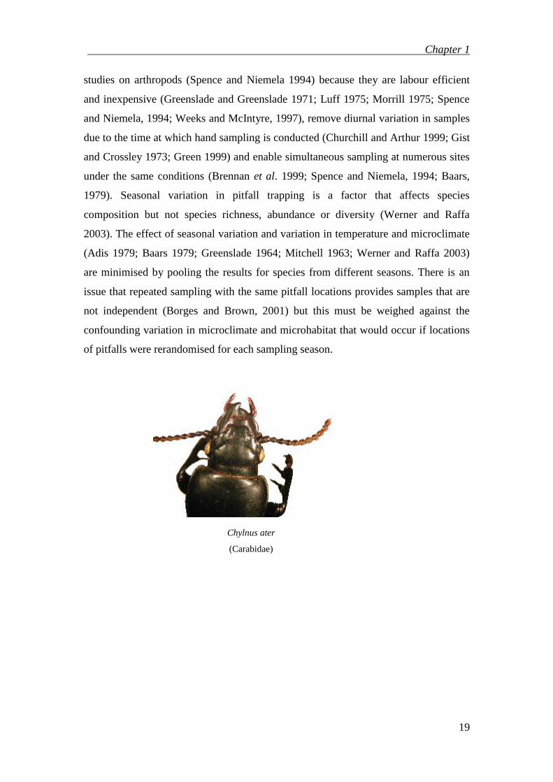
Chylnus ater
(Carabidae)

Chapter 1
20

Chapter 2
21
Material and Methods
4.1 Study sites
The study was carried out on two scales - intensive and extensive since variation in
invertebrate assemblages may be at such a small scale that even sites within
ecological vegetation classes differ as much as sites in different ecological vegetation
classes (Mac Nally et al. 2002). Small scale variation was studied in more detail. A
range of environmental variables were measured, including aspects of micro-climate,
fungal volumes and soil/litter attributes. These are described in detail later in the
chapter.
4.1.1 Location of study sites
The intensive study was carried out in the foothills of Mt Wellington, Hobart. The
study area of 1.3 km2 is bordered by Wellington Park to the West, suburban housing
to the North, and a Hobart City Council landfill buffer zone to the Southeast (Figure
2.1). Maps of study sites and distributions of the six eucalypt forest types in this study
were created using the open source GIS programme DIVA-GIS v 5.4, available on the
web from http://www.diva-gis.org with shapefiles for TASVEG v1.2 2005 available
from the Tasmanian Department of Primary Industries and Water.
The extensive study focused upon two of the forest types in the intensive study -
Eucalyptus pulchella and dry E. obliqua in each of 3 regions (Hobart, Levendale and
Swansea) (Figure 2.2), totalling 36 sites. The extensive regions, were 50 km apart,
spanning 157 km from Pelverata, south of Hobart, to Harding Falls near Swansea on
the east coast of Tasmania. The northern sites extended between the coast and the
Eastern Tiers, a range of Jurassic dolerite hills with podsolic soils, forested by
eucalypts (Harris and Kitchener, 2005) in woodland dominated by E. amygdalina and
E. pulchella with an open understory (Davies, 1988). The sites are all located within
the Tasmanian South East (TSE) IBRA bioregion (Figure 0.1). The distribution of the
six forest types across Tasmania are shown in Figure 2.3.

Chapter 2
22

Chapter 2
23
Figure 2.1 Location of Intensive study sites in the foothills of Mount Wellington
Figure 0.2 Location of Extensive study sites
HOBART
SWANSEA
LEVENDALE

Chapter 2
24
WRE Eucalyptus regnans forest
DOB E. obliqua dry forest
WOB E. obliqua forest with broadleaf shrubs
NOT YET MAPPED
DAM E. amygdalina on mudstone
DTO Eucalyptus tenuiramis forest on sediments
DPU Eucalyptus pulchella forest
Figure 0.3 Distribution of the six forest types sampled by this research (created from shapefiles

Chapter 2
25
for TASVEG v 1.2 2005)
Eastings and Northings for the location of each site are listed in Appendix 1. They
were originally recorded under the Australian Geodetic Datum 1966 (AGD66) but
have been converted to GDA94 datum. AGD 66 is being replaced with Geocentric
Datum of Australia 1994 (GDA94) to make it compatible with global navigation
systems such as the satellite-based Global Positioning System (GPS) which uses
World Geodetic System 1984 (WGS84) datum. The difference in origin between the
two datums is about 200m. If using a pre-2003 map published by TASMAP it will be
necessary to convert from GDA94 to AGD66 by subtracting 112m from each of
Eastings provided in this study and subtract 183m from each of the Northings. No
adjustment is required for a GPS set to GDA94 or WGS84
(http://www.icsm.gov.au/icsm/gda/). Since many of the maps in use are based on the
older AGD66 system, both types of data are provided in Appendix 1 for the sites in
this study.
4.1.1 Selection of Eucalypt Forest types
TASVEG v1.2 2005 (DPIWE, 2005) provided mapped forest communities from
which it was possible to select six adjacent eucalypt forest types. The study area of
1.3km2 contained four replicates of each forest type, totalling 24 sites. Table 2.1 lists
the forest types and the site numbers within each forest type.
FOREST TYPE RFA
(TASVEG
2000 CODE)
TASVEG v1.2
COMMUNITY
CODE 2005
SITE NUMBERS
Mt Wellington
(MW)
Eucalyptus regnans forest R WRE 1, 2, 3, 4
Eucalyptus obliqua forest with broadleaf shrubs OT WOB 5, 7, 12, 16
Eucalyptus obliqua dry forest O DOB 6, 8, 17, 20
Eucalyptus tenuiramis forest on sediments TI DTO 9, 10, 19, 21
Eucalyptus pulchella forest P DPU 11, 13, 18, 24

Chapter 2
26
Eucalyptus amygdalina forest on mudstone AI DAM 14, 15, 22, 23
Table 2.1 Forest types sampled in the study
The proximity of sites to each other minimised variation due to climate, fire events,
landscape, geology and soil. Each site was a minimum of 5 m away from tracks to
minimise disturbance. It must be noted, however, that presence of certain vegetation
types is a result of variation in geology and topography so the location of forest type
was not a random variable in the research. For example, the leaves of E. pulchella are
well adapted to dry conditions and on Mt Wellington it is found on steep, north
facing, shallow, dry soils on Jurassic dolerite, particularly ridge tops (Reid and Potts
1999). E. tenuiramis occurs on steep north facing slopes of Permian mudstone while
E. amygdalina occurs on steep north facing slopes of Triassic sandstone. All three of
these eucalypt species are replaced by E. obliqua on cooler and wetter south facing
slopes, regardless of the underlying rock type ( Reid and Potts 1999; Williams 1991).
E. globulus and E. regnans are found on deeper, moist, well drained soils.
Four of the monocalypts selected in this study were singularly dominant in their forest
type: E. obliqua, E. regnans, E. amygdalina and E. tenuiramis. As is typical for
Symphomyrtus species (Reid and Potts 1999), E. globulus and E. viminalis were co-
dominant with a monocalypt, E. pulchella. Co-occurrence of a monocalypt with a
symphyomyrt is typical of forests linking dry sclerophyll to moist forests where Ashes
such as E. obliqua and E. regnans dominate (Duncan 1999). Harris and Kitchener
(2005) provide descriptions of the mapped Tasveg v1.2 forest types that are listed in
Table 2.1. Photos of the sites, displaying variation in understory cover, appear in
Figure 2.4.

Chapter 2
27
WRE Eucalyptus regnans forest, site 3 WOB Eucalyptus obliqua forest with broad leaf shrubs,
site 16
DOB Eucalyptus obliqua dry forest, site 17 DTO Eucalyptus tenuiramis forest on sediments,
site 19
DPU Eucalyptus pulchella forest, site 13
DAM Eucalyptus amygdalina forest on mudstone, site 15
Figure 2.4 Site photos representing the variation between forest types.

Chapter 2
28
4.1 Sampling of spiders and beetles
4.2.1 Experimental design
A stratified random pitfall sampling regime based on forest type was employed for the
Mt Wellington sites. Four sites within each of six adjacent TASVEG Vegetation types
were surveyed for beetle and spider species using 10 pitfall traps at each site during
three seasons.
Pitfall traps were used in this study to assess relative abundance of beetles and spiders
in different eucalypt vegetation types. Small diameter (4.2 cm) plastic traps were
selected to reduce impact on larger non-target species such as frogs and lizards. Traps
were located within a 200 m2
area at each site. Ten pitfall traps were placed at 10m
intervals along two 40 m rows that followed a contour. Each row was 5 m apart.
Each pitfall trap was buried to ground level so that the top was flush with the soil and
half filled with Gault’s solution containing a small quantity of chloralhydrate as
follows: sodium chloride 50g/l, potassium nitrate 10g/l, chloralhydrate 10g/l, and
glycerine 20ml/l.
Figure 0.5 Pitfall trap design used in sampling
Gault’s solution was selected by Meeson (2006) when establishing the sites for
pitfall trap containing Gault’s solution. 4.5cm
ground level
plastic lid
wooden skewers

Chapter 2
29
research on ants but it was later found to be a poor preservative for spiders (Vink
2002).
A 10 cm plastic lid was secured as a roof over the trap with two wooden skewers
pushed into the ground. The lid was tilted for rain run-off (Spence and Niemela 1994)
and was covered with small pieces of bark and leaves to camouflage it from ravens
and other birds as well as to reduce evaporation of liquid in the traps (Figure 2.5). Lid
transparency has been shown to have no microclimatic effect that biases pitfall
catches towards, for example, carabid beetles (Phillips and Cobb 2005).
Each trap remained open in the field for twenty-five days. For the intensive study in
the Mt Wellington foothills, sampling was conducted in spring (November 2002),
summer (February 2003) and autumn (April 2003). Sampling for the extensive study
was conducted in spring (November 2003).
Once ants had been removed by Meeson (2006), pitfall catches from all 10 pitfall
traps at a site were pooled into one container for sorting and identification of beetles
and spiders, although this resulted in loss of information for later analysis.
4.2.1 Identification of species and morphospecies
Spider and beetle specimens collected in the pitfall traps were identified to
morphospecies and later identified to species level where possible with assistance
from Dr Peter McQuillan (Coleoptera) and Bec Harris and Lisa Boutin (Araneae).
Access to the Department of Primary Industries and Forestry Tasmania insect
collections enabled further identification of Coleoptera, while Liz Turner provided
access to the Tasmanian Museum and Art Gallery spider collection.
An extensive file of original descriptions of species was compiled and for large
families with many unnamed species, matrices of characteristics that distinguished
species were developed. A reference list of taxonomic literature used for identification
appears in Appendix 7. Species were photographed and a voucher collection was
deposited at the University of Tasmania in the Biogeography Fauna Laboratory of the
School of Geography and Environmental Studies.

Chapter 2
30
Biophysical attributes
4.2.1 Aspect/Altitude/Slope
Altitude, aspect and slope were recorded as continuous variables. Altitude was
determined in metres from the 1:20,000 series of maps. Aspect to the nearest 10
degrees was measured with a compass and slope was measured in degrees using a
clinometer.
A table of the site characteristics are presented in Appendix 1.
4.2.1 Soil
The focus of this study is on litter invertebrates, but owing to overlap of species in soil
and litter microhabitats (Coy et al. 1993) it was necessary to include soil variables as
possible factors that may influence invertebrate assemblages collected from litter.
4.2.4.1 Soil Hardness
Soil hardness was measured as resistance to penetration. It varies with soil type and
increases with higher bulk densities, while it decreases with increasing water content
and increases with decreasing particle size due to lower matric potential which is a
measure of the strength with which the soil holds water (Bengough et al. 2001).
An Ele pocket penetrometer with a cylindrical tip of 0.6 mm was used in the field to
measure soil strength (resistance to penetration) as unconfined compressive strength
of the sample in kgf/cm2
on a scale from zero to five. (Shear strength equals this
reading divided by 2). A wider tip of 26 mm inserted to the same depth of 0.6 mm
was used to increase accuracy for softer soils where readings were close to zero.
When the penetrometer encountered a stone the result was discarded and the
measurement was repeated nearby to reduce outlier data that would bias comparisons
across sites (Bengough et al. 2001).

Chapter 2
31
A minimum of seven independent replicate measurements were required based on
formula (1) (Bengough et al. 2001) for a 95% confidence interval (ASAE, 1969).
N=[ 2CV] 2
L 2
…………………….. (1)
Where N = number of required measurements (N) taken at least 1 metre apart; L = the
95% confidence interval as a percentage of the mean and CV = the coefficient of
variation.
In total, fifteen replicate penetrometer readings at randomly located distances greater
than 2 m apart were recorded for each site in winter and the following summer. Soil
hardness was recorded as a continuous variable.
4.2.4.2 Chemical analysis of soil
To collect samples, the litter layers (undecomposed O1 horizon and decomposing O2
horizons) were swept aside and a soil core of 5 cm diameter x 10 cm deep was taken
using an aluminium tube which was twisted by hand into the soil. The depth of the
topsoil (A horizon) and subsoil (B horizon) in the core was recorded. The topsoil and
subsoil were placed in separate containers. Additional cores of each horizon were
taken from adjacent soil until a 500 cm3 container was filled to provide enough
material for measuring moisture content and chemical analysis. Six independent,
random replicates of each horizon were collected at each site at distances greater than
five metres apart. Containers were immediately sealed and kept cool (Rayment and
Higginson 1992) to prevent water loss and minimise chemical changes prior to
analysis.
Samples for chemical analysis were collected in summer and air dried in a laminar
flow cabinet so that samples would remain cool and could dry as quickly as possible
to reduce chemical change.
Air dried soil was sieved to remove gravel and particles > 2 mm. Sieved samples were
Chapter 2
32
ground with a mortar and pestle and sieved through 0.5 mm mesh ready for chemical
analysis.
The nitrogen, phosphorus and organic carbon content of the soil was determined using
methods described by Rayment and Higginson (1992). For example, available
Phosphorus was measured by the Bray extractable phosphorus method which extracts
phosphorus compounds soluble in acid. The carbon to nitrogen (C:N) ratio was
calculated from the values of available carbon and nitrogen. Available rather than
total chemical content was a more relevant measure of soil chemicals since it is a
measure of the amount of a chemical available to biotic components such as plants
and microbes on the forest floor (Vesterdal 1998).
4.2.1 Soil pH
Tests for soil pH were carried out in the field to prevent error due to alteration of pH
during transport from biological activity, temperature increase and chemical change
(Brower et al. 1989). A kit by Inoculo Laboratories, Victoria, was used where a small
soil sample was mixed with indicator solution, then dusted with white barium
sulphate powder. This allowed the colour of the pH solution to become visible and be
matched against a colour chart to determine the pH within an accuracy of half a pH
unit. Five random samples were measured for soil pH at each site and the results
averaged for each site.
4.2.1 Microclimate
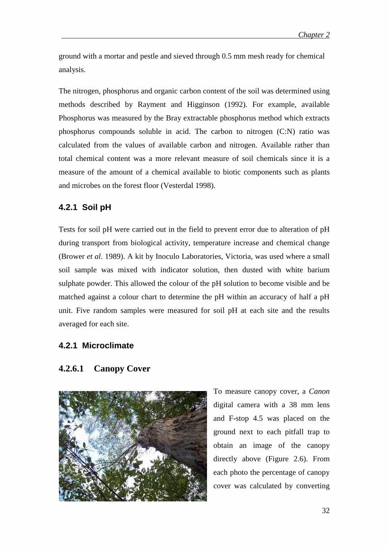
4.2.6.1 Canopy Cover
To measure canopy cover, a Canon
digital camera with a 38 mm lens
and F-stop 4.5 was placed on the
ground next to each pitfall trap to
obtain an image of the canopy
directly above (Figure 2.6). From
each photo the percentage of canopy
cover was calculated by converting

Chapter 2
33
each photo to grey scale, pixellating each photo and assessing each pixel as either
black (canopy) or white (no canopy). The advantage of this method was that it
provided a measure of penetration of solar radiation adjusted by canopy and sub
canopy density. A categorically scored canopy cover index would have under-
estimated solar penetration by ignoring the effect of the pendulous nature of eucalypt
leaves (Baehr 1990).
Figure 2.6 Sample photo of the canopy taken from ground level for site 4, from which average
percentage of canopy cover was calculated.
4.2.6.2 Solar Radiation
Solar radiation and adjusted solar radiation were determined for summer and winter.
Solar radiation was determined using Nunez’s estimation of solar radiation received
on slopes in Tasmania (Nunez 1983, p. 156-157) from equation (2).
Incoming solar radiation (KC↓) = direct radiation on surface + diffuse radiation from the sky
incident on the surface + diffuse radiation from reflection of global
radiation by the ground.
KC↓ = Io τ cos γ + D .VF + Gc α (1-VF)
…………………(2)
where: Io = solar constant = 1353 Wm-2
τ = the transmission of the atmosphere to direct radiation
γ = the angle of incidence of direct radiation with the inclined surface
(cos γ = sinZ.cosф.sinX.cosY + sinZ.sinф.sinX.sinY + cosZ.cosX
where Z, ф = zenith and azimuth angles for direct solar radiation;
X,Y = zenith and azimuth angles for the normal to the surface)
D = diffuse radiation incident on a horizontal surface = 0.6Wm-2

Chapter 2
34
VF = the sky view factor (from 0.5 for a vertical surface to 1 for horizontal)
α = albedo of the surface (a mean of 0.2 between eucalypt forests and dry grasslands
was used)
Gc = global solar radiation on a horizontal surface = Io τ cos Z + D (Z= solar zenith
angle)
Estimations of summer solar radiation for southern Tasmania range from a maximum
of 22.0 MJm-2
per day on a horizontal surface in December to 9.0 MJm-2
per day on a
vertical south facing slope. In winter solar radiation reaches a maximum of 9.0 MJm-2
per day on a north facing slope of 65o and falls to 1.9 MJm
-2 per day on a vertical
south facing slope (Nunez 1983).
Aspect and slope data for each study site enabled an estimation of solar radiation to be
read from Nunez’s (1983) charts.
Nunez’s model applies to bare ground. An innovation of this study was to adjust the
solar radiation figure to provide a value for the amount of radiation falling on litter
under a canopy. This entailed multiplying solar radiation (Nunez, 1983) by the
percentage of non-canopy cover.
Adjusted solar radiation represented the solar radiation incident on the litter layer
beneath the canopy.
Adjusted solar radiation = solar radiation x (100 - % canopy cover measured
from the litter layer)/100
……….…………(3)
4.2.6.3 Sub-soil and Ground Surface Temperatures
Soil temperature may be considered to be an index of canopy cover, litter depth and
soil moisture and thus it is expected that a correlation will exist between this data. To
measure suface litter or bare ground temperature, a Raytec Lasar Temperature Gun
was directed at a randomly selected spot on the ground and scanned over an area of

Chapter 2
35
half a square metre for three seconds. The temperature gun was set to display the
average temperature during that time and this was recorded. This was repeated until 5
readings for litter covered surfaces and 5 readings for bare ground were obtained.
Each set of 5 readings was averaged to provide an average surface temperature for
litter cover and bare ground at each site. Not all sites had both litter cover and bare
ground so only relevant recordings were made. Measurements were made for each site
during summer and winter. Results are recorded in Appendix 6.
Sub-soil temperatures were taken at 5 cm below the surface by digging down 5 cm
with a spoon and immediately directing a Raytec temperature gun at the lowest point
of soil. Ten measurements were recorded and averaged for each site. Measurements
were conducted during summer and winter.
4.2.6.4 Surface Air Humidity
A TempTec instrument was used to measure air humidity at ground level. Five
readings at each site were averaged to provide an average measure of humidity for
each site. All readings were done during the morning on the same day to minimise
variations in weather conditions between sites and provide a rough measure for
comparison across sites.
4.2.6.5 Soil Moisture
Since soil moisture varies according to rainfall, drainage, waterholding capacity of the
soil and evapotranspiration (Brower et al. 1989) a full profile of soil moisture requires
multiple sampling across seasons. This study was only able to provide a single
snapshot to compare relative soil moisture across sites. Six separate randomly
selected, replicate samples were collected at each site for individual analysis. This

Chapter 2
36
was preferable to the common practice of pooling six soil samples and then
subsampling six times from the pooled samples for each site (Hanna 1964) since it
would provide information on the variation of soil moisture within a site. Soil
moisture was measured from the soil samples collected for chemical analysis (section
2.2.4.2).
To calculate the percent water content of soil, a thermogravimetric method for soil
water content was used. Water held by surface tension was evaporated from a
weighed soil sample, with gravel and rocks > 2 mm removed (Rayment and
Higginson 1992), in an oven at 105 o
C for about 24 hours until no further change in
mass occurred (Gardner et al. 2001; Brower 1989), i.e. where, under procedures of the
International Standards Organisation, during a further 4 hours of drying the mass
difference was not greater than 0.1% (ISO 1993). Rather than cool soil in a desiccator
before weighing, each sample was weighed while hot from the oven to reduce
moisture uptake. The loss of weight represents moisture content and is expressed per
100g of dry soil:
Soil moisture = (wet weight - dry weight) x 100% / dry weight
……………..(4)
It must be noted that not all water is removed at 105 oC. Adsorbed and structural water
are not removed until 110-160 oC and 400-800
oC respectively so they are traditionally
not included in measures of soil moisture. Some error may also be introduced for
organic soils that may lose other components apart from water at 105 oC (Gardner et
al. 2001).
4.2.1 Ground Cover
Four intercept transects were conducted at each site The method was to proceed a
randomly selected number of paces along the site from the first pitfall trap and carry

Chapter 2
37
out a 20 m intercept transect in a randomly selected direction 10m forward and 10 m
backwards from that point. Ground cover was recorded at 10 cm intervals and
classified as litter, bare ground, rock, coarse woody debris, grass, shrubs, herb, tree
(eucalypt), tree (understorey), fern, tree (sapling), understorey tree (sapling), mossy
rock, mossy coarse woody debris, mossy tree (eucalypt), mossy tree (understorey).
Results of the transects were averaged for each site.
4.2.1 Litter Depth
Litter depth data was obtained from five transects at each site by proceeding a
randomly selected number of paces along the site from the first pitfall trap and
marking out a transect in a randomly selected direction 10 m forward and 10 m
backwards from that point. Five measures of litter depth were obtained for each
transect by taking a measurement at 4 m intervals. Where intercept transects were
being conducted litter depths were measured concurrently along the same transects.
4.2.1 Rotten wood volume
Fixed-area plot sampling was undertaken in randomly located plots of 250 m2
(50 m x
5 m) in which the volume of all rotting logs was calculated.
4.2.1 Basal Area
The Basal Area of trees at each site was estimated using the Bitterlich method named
after the Austrian forester who developed it in the 1930s (Brack and Wood 1997) with
point sampling. A Bitterlich Wedge, consisting of a wooden crosspiece gauge was
held at arm’s length over a randomly chosen spot within the site and rotated
horizontally 360 degrees over the spot while the number of trees with breast height
equal to, or greater than the width of the crosspiece from that distance, were counted
and recorded as m2/ha. Using a rod of length 50 cm with a crosspiece of 1 cm
provided a 50:1 ratio so that the direct count of trees was equal to the basal area in
m2/ha. The stick was held parallel to the ground to compensate for slope effect which

Chapter 2
38
would cause an underestimation of number of trees.
This procedure was conducted five times from random locations at each site. The
resulting 5 scores were averaged to provide the mean basal area of trees in square
metres per hectare for that site.
4.2.1 Plant Communities
Major vascular plant species identified during a 20-minute survey of each site were
recorded and abundance assessed using the Braun-Blanquet score where a score from
1 to 5 was assigned to each species in that vegetation type according to its percentage
of coverage of the site.
Braun-Blanquet score Species cover %
1
< 1%
2 1-5%
3 6-25%
4 26-50%
5 51-75%
6 76-100%
Table 2.2 Braun-Blanquet score for vegetation cover
4.2.1 Fungi
A snapshot sample of fungi species was provided by recording the species and volume
of macro fungi above the ground at each site during autumn (May). The volume of
each fruiting body was calculated from measurements taken of the diameter and depth
of the pileus (cap) and diameter and length of the stipe, where relevant. Photographs
were taken to aid identification from reference books (Fuhrer, 2001; McCann, 2003)
and from the expertise of Sapphire McMullan-Fisher.

Chapter 2
39
4.1 Statistical analysis
4.3.1 Diversity in species assemblages among sites
Diversity is an index of the variety (species richness) and relative abundance
(evenness) of species in a sample (Magurran 1988).
Species turnover, which refers to change in species diversity along an environmental
gradient (Vellend 2001) was not calculated as the sites were not ordered a priori, but
a more general measure of beta diversity was calculated from the large number
available to measure of the change in species among sampled sites.
Local variation in beta diversity among adjacent forest types was investigated by
comparing species richness using a modification of Whittaker’s beta biodiversity
index (Harrison et al. 1992). The modification allows for uneven numbers of samples
by dividing Whittaker’s Index by the number of sites minus one and expressing the
result as a percentage.
x [(S / ) – 1] / (N – 1 ) …………………………….(4)
N = number of sites
the maximum number of species recorded at a site
S=the total number of species in the study
The index ranges from 0 (completely similar) to 100 (completely dissimilar).
Fundamental to the choice of appropriate statistical tests was the undertaking of
exploratory data analysis. Scatterplots of combinations of pairs of variables were used
to identify correlations that may interfere with some analyses, as well as to check the
normality of the data, homogeneity of variance and sample distribution so that outliers

Chapter 2
40
that may require log transformation of the data could be identified.
4.3.1 Looking for patterns in species assemblages among sites
A preliminary NMDS ordination of dissimilarity of species distribution across sites
was conducted to see which sites clustered together in species space due to shared
species and whether these clusters corresponded to forest type. If identifiable
groupings could be discerned, then more rigorous tests could be conducted to
determine whether any of the measured environmental variables contributed towards
the assemblage patterns.
4.3.1 Do assemblage patterns correspond to forest types?
More rigorous investigation of the relationship between patterns in beetle and spider
distributions and forest type was provided by non-parametric multivariate analysis of
variance and analysis of similarity to test the null hypothesis that the means of the
assemblages grouped by forest type are not different in their multivariate means or in
their dispersion. The purpose was to determine whether species from the same forest
type are more similar than those from different forest types. In addition, a posteriori
pairwise tests were conducted to compare which forest types had significantly
different assemblages to other forest types. The NPMANOVA (Anderson, 2003)
programme was used for beetles and spiders in the local scale Mt Wellington study,
which was a one-way simple ANOVA design. PERMANOVA (Anderson, 2005) was
appropriate for the two way crossed factor design of the more extensive regional
study. NPMANOVA and PERMANOVA have been applied to analyses of beetles in
wildlife habitat strips (Grove and Yaxley 2005), edge effects on beetle (Baker et al.
2007; fauna inhabiting kelp holdfasts (Anderson et al. 2005) and a re-analysis of
intertidal gastropods (McArdle and Anderson 2001).
PERMANOVA and NPMANOVA provide a semi-parametric multivariate analysis of

Chapter 2
41
variance that simultaneously compares group centroids for a linear model. The
programmes were developed to overcome the limitations of ANOSIM and are freely
available from http://www.stat.auckland.ac.nz/~mja/Programs.htm. By calculating
variance as the Sums of Squares (SS) of distances from observations to centroids, a
variety of distance measures can be used apart from Euclidean, thereby avoiding the
limitations of a multivariate ANOVA (MANOVA) analysis of several dependent
variables where there are many zeroes in the data (Field et al. 1982; Legendre and
Legendre 1998).
NP-MANOVA analysis of the Mt Wellington data was conducted for a one-way
design to compare species recorded in each of the different forest types with sites
grouped by forest type (6 factors) and 4 replicates of each. PERMANOVA analysis of
the more extensive regional sites was conducted for a two way crossed model for
fixed factors ‘region’(3 levels) and ‘forest type’ (2 levels) with 6 replicate sites for
each. For both analyses data were fourth root transformed, a severe transformation to
overcome the large differences in abundances from hundreds for some species to
zeroes for many others. Distances between pairs of samples were calculated using the
Bray Curtis dissimilarity measure which is appropriate for data with many zeroes
because it does not count joint absences as similar (Clarke et al. 2005; Clarke and
Ainsworth 1993; Field et al. 1982).
From the dissimilarity matrix the sum of squared distances among groups in the half
matrix, divided by the number of samples yielded the total sum of squares (SST):
SSN
dT ij
j i
N
i
N
1 2
11
1
…………………….(5)
Similarly, the sum of squared distances within groups (SSW) was calculated by
dividing the sum of squared distances between replicates in the same group by the
number of replicates in that group:
1
1 1
21 N
i
N
ij
ijijW dn
SS …………………..(6)

Chapter 2
42
for ij =0 if observations i and j are in the same group and 1 if they are in different
groups (Anderson, 2001). The among group sum of squares could then be calculated
as
SSA = SST - SSW …………………..(7)
A pseudo F-ratio test statistic for the factor ‘forest type’ was calculated as a ratio of
the sum of squared distances among groups and the sum of squared distances within
groups:
F = SSA / (a-1) ………………….(8)
SSW/ (N-a)
where a = number of groups, n= number of replicates, N = number of samples = a x n
The test statistic was a pseudo F-ratio because a non-Euclidean distance measure
(Bray-Curtis) was more appropriate for the data and the variables may not be
normally distributed, making standard F tables inappropriate (Anderson 2005). Under
these circumstances a permutation procedure was used to randomly reallocate samples
to any forest type to test a null hypothesis for no effect of forest type by calculating an
Frandom-ratio for all possible random combinations of samples (shuffling of rows) in
the original data matrix. The Frandom value of the permutations was compared with
the experimentally derived F-ratio to determine a P value (Anderson, 2005):
P = Number of Frandom ≥ F ………….(9)
Total number of Frandom
The distribution of the F ratio under the null hypothesis of no difference between the
treatment groups was compared to the observed F-ratio. The Frandom value was
derived from 9999 unrestricted permutations of raw data. If any of the main effects
were significant, a posteriori pairwise comparisons of variables were requested and
the significance of the pairwise tests for differences between assemblages in different
forest types were corrected for multiple comparisons using sequentially adjusted
Bonferroni probabilities.

Chapter 2
43
A non-metric MDS plot of 4th
root transformed abundance data with Bray-Curtis
distances was created in ‘R’ to provide a visual indication of variation in the data.
PERMANOVA and NP-MANOVA can indicate that a difference between groups is
significant if there is a variation in spread among groups with some groups widely
dispersed and others clumped (Anderson 2003, 2005). Therefore, if a significant result
was obtained from PERMANOVA or NP-MANOVA analyses, investigation was
undertaken to determine whether the significant difference between groups was due to
dispersion differences among groups or to location (Anderson, 2004). To do this, a
programme called permutational analysis of multivariate dispersions (PERMDISP)
(Anderson, 2004) was used to test the homogeneity of the data by comparing the
multivariate dispersion among groups of the Bray-Curtis dissimilarity measure. The
PERMDISP programme calculates distances of observations from their centroids and
then uses an ANOVA procedure to compare the average of the distances among
groups (Anderson, 2004). Through the programme’s use of distances of observations
from centroids, a variety of distance measures can be used apart from Euclidean
distance.
While it is preferable to use Euclidean distance as a distance measure to preserve the
centroid as the arithmetic mean of the original observation and the variable in
PERMDISP analysis, the Bray-Curtis distance measure was selected to retain
consistency with the distance measure used in the NP-MANOVA analyses. This
enabled a comparison to be made with the original analysis. Similarly, transformation
of abundance data to fourth root was selected for consistency with the NP-MANOVA
tests even though transformation affects the heterogeneity of the data which in turn
affects dispersal of points which is what was being examined. A total of 9999
permutations of the raw data were used.
PERMDISP made it possible to tease out whether significant results for differences in

Chapter 2
44
species assemblages in different forest types in PERMANOVA were due to location
and/or relative dispersal of the data.
In a similar vein to nonparametric multivariate analysis of variance, an analysis of
similarity (ANOSIM, Clarke 1993) was conducted to test whether the grouping of
beetle assemblages by forest type resulted in more similarity within forest types
compared with between forest types. The procedure has been used to analyse
associations between matrices of species (Gibb and Hochuli 2002; Major et al. 1999;
Murray et al. 2006; Somerfield et al. 2002).
The null hypothesis tested was that the distances between pairs of samples between
groups were the same as the distances between pairs of samples within groups. The
technique used a non-parametric permutation technique on a Bray-Curtis dissimilarity
matrix transformed into a matrix of rank similarities where the elements were ranked
so that the highest similarity has the lowest rank of one. The aim was to test for
differences in species assemblages in the a priori grouping of forest type.
An R statistic was calculated for the observed data:
_ _
R = ( rb - rw ) ………….(10)
(M / 2) _
where rb is the average of all pairwise rank similarities between site
rw is the average of all pairwise rank similarities among replicates within sites
for M = n(n-1)/2 where n is the number of samples
A second R statistic was calculated for each permutation of labels randomly
reallocated to a different sample and the distribution of this R statistic under the null
hypothesis of no difference between forest type was compared to R for the real data.

Chapter 2
45
(4 replicates of 6 treatment groups gave 4.5E+12 permutations so 10,000
permutations were conducted).
The null hypothesis was rejected at a significance level of 100 x (t+1)/(T+1) % where
t is the number of simulated R ≥ observed R and T is the total number of simulations.
ANOSIM is sensitive to zero inflated data, so species whose abundance was less than
5 were excluded. This is unlikely to affect the results since species with low
distributions are unlikely to be present at enough sites to affect the results. The
resulting boxplots portrayed the dispersal of the data.
4.3.1 Detecting environmental variables in assemblage patterns
Rank dissimilarity between sites was mapped to determine whether there might be
any groupings of sites by similar variables and whether these groupings corresponded
to forest type.
An exploratory NMDS of species distributions was overlaid with environmental
variables represented by different sized circles to visually compare whether their
variation corresponded to species distributions. Forest type was excluded from the
variables in order to detect patterns arising from other variables.
Canonical Analysis of Principal Coordinates (CAP) (Anderson, 2004) was conducted
to provide a measure of the contribution of each environmental variable to the
variation in the species data, thereby examining how assemblages vary across
environmental gradients (Baker et al. 2007; ter Braak 1986). This enabled the
variables with the greatest influence on the data to be identified and provided a basis
for selection of a smaller number of variables for further analyses using the
permutational selection procedure, BIOENV. CAP was employed in preference to
Principal Components Analysis (PCA) which assumes multivariate linearity of the
data (Anderson and Willis 2003; Kempton 1977; Legendre and Anderson 1999;
Palmer 1993; ter Braak 1986).

Chapter 2
46
CAP provided a canonical analysis of the effect of the matrix of environmental
variables (standardised) on the species variables (transformed to ln+1). A reduced set
of environmental variables was used to constrain the ordination since use of all
environmental variables would have provided an unconstrained analysis similar to an
NMDS. Bray-Curtis dissimilarities were centred to generate a Gower’s centered
matrix from which an eigenanalysis provided eigenvalues which were the squared
canonical correlations of the matrix from which the test statistic, the greatest root
statistic, δ2, was calculated. The p value for the statistic was the result of permutations
of groups, with 9999 permutations selected. Visual support for the results was
provided by plotting the eigenvectors from the principal coordinates analysis (PCO
axes), as an unconstrained MDS (Anderson, 2004).
4.3.1 Detecting which environmental variables are important
If a difference between assemblages in different forest types was established
exploratory analysis of environmental variables was undertaken to identify which
environmental variables might be important to the distributions of invertebrates
(De’ath 2002; Moore et al. 1991; Woehler et al. 2003). Regression tree models were
built in R (version 2.4.1) using the tree package (Ripley, 2007) to determine which of
the numerous environmental variables measured were important to beetle and spider
distribution. Regression trees were appropriate because the species data are
continuous, although analyses assume that data are normally distributed. Histograms
of species data (abundance vs frequency) was used to verify this normality. (Moore
1991)
Regression trees employ a nonparametric, iterative method that partitions multivariate
data dichotomously into ranked subsets based on the differences among a priori
groups. Partitions are selected by the programme where they minimise deviance in the
data. In the output trees, the improvement in prediction error obtained by the split is

Chapter 2
47
proportional to the depth of the tree below each split. At each node the variable that
distinguishes best between observations is identified along with the value at which the
split occurs. The leaves of the tree display the mean number of species present in that
particular split of the data.
Before building regression trees, rarer species (less than 5 individuals present in the
whole dataset) were removed from the species matrix since their occurrence was not
significant enough to detect patterns with environmental variables. All environmental
variables were used.
PCA was used to identify variables that described most of the differences in
environmental variables between sites. The function BIOENV (Clarke and Ainsworth
1993) was applied to the question of which environmental variables had a significant
role in explaining the variability of species distributions rather than site variation.
BIOENV was appropriate for comparing two matrices of variables (biological and
environmental) to explore which variables were significant. It has been more
commonly applied to marine and freshwater analyses of assemblages (Clarke 1993;
Frost et al. 1999; Whitman et al. 2004).
BIOENV sought the best subsets of environmental variables by estimating the
correlation between ranked Bray-Curtis dissimilarity among species and ranked
Euclidean dissimilarity among standardised environmental variables for the sites. It
sequentially added variables to the predicted model that would provide the highest
Spearman rank correlation between elements of the two dissimilarity matrices (Clarke
and Ainsworth 1993). The BIOENV procedure in the Vegan package (version 1.8-5,
Oksanen et al. 2007) for ‘R’ takes some time for large numbers of variables, in this
case 256
– 1 = 7.2 x 10¹⁶
permutations. Therefore variables were first reduced, based
on information from other analyses and removal of redundant correlated variables.
BIOENV enabled a further reduction of the number of most important environmental

Chapter 2
48
variables which was required before further investigation of variation could be
explored.
If there was an indication that vegetation type was a significant variable for
distributions of species, a hierarchical partitioning (Chevan and Sutherland 1991)
method of multiple regression was used to jointly compare all possible models and
identify variables that are independently correlated with species distribution
responses. The leaps version 2.7 package in ‘R’ was used, for which computation is
relatively quick because the method uses a branch and bound (Hocking and Leslie
1967) or leap and bound algorithm (Furnival and Wilson 1974; Lawler and Wood
1966) to calculate the residual sums of squares so that every set does not need to be
considered. The programme computes a maximum of 31 variables at a time, however,
the number of variables must be less than the number of observations otherwise the
lower bound is uniformatively close to zero. The default options for selection of
models that assume there is a linear, Gaussian model, are R2, adjusted R
2 or Mallows
Cp. The program was modified to use a non-parametric cross-validation PRESS
(prediction sum of squares) statistic (Allen 1974; Miller 1990).
4.3.1 Spatial variation
The influence of geographic distance between sites on similarity of assemblages,
referred to as autocorrelation, was investigated using the Mantel test in the Vegan
package (Oksanen et al. 2007) in ‘R’ which for which Spearman’s rank correlation for
non-parametric data was used. The distances between a Bray-Curtis matrix of
dissimilarity in species abundance for pairs of sites and a second matrix of geographic
distances between pairs of sites were compared. The null hypothesis was that the
distribution of one matrix was independent of the components of the other. A Monte
Carlo permutation test for significance of the correlations calculated a statistic for the
frequency of randomised correlations that were at least as strong as the observed
correlations. A lower test statistic was more significant i.e. the distribution of one
matrix was independent of the other which means that sites located closer together
were not more similar than sites located further apart.

Chapter 2
49
It must be noted, however, that the Mantel test used in this way is not suitable for
questions about the raw data because it partitions the variation in a dissimilarity
matrix. Variation of the dissimilarity (sums of squares) of a distance matrix is not a
measure of beta diversity of the species among sites (Legendre et al. 2005). For this
reason canonical analyses which partition the variation in species abundance data are
able to explain a greater amount of total variation than the Mantel test which can only
be applied to variation in groups of sites. Canonical analyses were therefore adopted
for an examination of distance by partitioning variation as used by Borcard 1992;
Cushman and Wallin 2002; Okland and Eilersten 1994; Oliver et al. 2000.
4.3.1 How much of the environmental and spatial variation explain
species distributions?
Having identified spatial and environmental factors that corresponded to species
distributions, it was possible to explore the amount of variation explained by each
data matrix through partitioning of variation using partial canonical ordination. The
method has been used to study assemblages of ants (Debuse et al. 2007), orbatid mites
(Borcard and Legendre 1994) and plants (Ohmann and Spies 1998). Partitioned
components were: environmental, spatial, the spatial component of environmental
variation and undetermined.
Canonical correspondence analysis (CCA) combines multivariate ordination and
simple multiple regression. The species ordination axes are constrained to be linear
combinations of the environmental variables of the second matrix to provide an
optimal relationship between the two.
CCA was first run with all environmental variables, then with partitioning of
variation. Steps in the process are based on Anderson and Gribble (1998), Legendre
and Legendre (1998) and Borcard et al. (2004).
Three matrices were required for the analysis, the first being a species matrix where
species with an overall abundance less than 5 had been removed. Secondly a matrix
Chapter 2
50
of a reduced number of environmental variables was necessary for Canonical
Correspondence Analysis which is a constrained ordination. Redundant variables had
been identified in earlier analyses such as NMDS, CAP and BIOENV and could
further be identified through multiple regression using a forward stepwise selection
procedure. It was also necessary to remove correlated variables.
The third was a Principal Coordinates of Neighbour Matrices (PCNM) matrix
representing spatial variation of the species data (Dray et al. 2006). A PCNM was
selected for modelling spatial components of variation in preference to a trend surface
polynomial function of the centred coordinates of sites. PCNM has been found to
provide a more realistic representation of the spatial components of species variation
(Borcard 2002) and also enables this variation to be represented at different scales
(Borcard and Legendre, 2004). This was an important consideration in this research
for which species data were collected across two different scales. In addition,
environmental variables that are categorical and therefore not additive, such as Braun-
Blanquet scores of vegetation cover and aspect are not well represented by trend
surface analysis which develops an area-wide regression model from which the values
of variables at particular locations are predicted. Higher degree polynomials may be
more representative of spatial complexity but reduce the degrees of freedom of the
model (Legendre and Legendre 1998).
PCNM variables are principal coordinates of a truncated matrix of geographic
(Euclidean) distances. The matrix of PCNM variables was created from a file of
Cartesian coordinates (eastings and northings) using Spacemaker2 (Borcard et al.
2004), an open source programme available on the web from
http://www.bio.umontreal.ca/legendre. Creation of a truncated matrix required input
of the smallest truncation distance that would be large enough to join all sites.
Relative neighbourhood graphs produce a minimal number of edges when connecting
all points and were the graphing method used in R (version 2.4.1) to determine the
truncation distance of 431 m which became the finest scale at which PCNM analysis
could analyse the data. If desired, the analysis could be rerun at a finer scale by
adding supplementary data points. The maximum distance across the whole study
area was 1757 m, and this set the limit for the largest scaled PCNM variable’s

Chapter 2
51
wavelength.
The Spacemaker2 programme created the truncated distance matrix in which
distances greater than the input value of 431 m were transformed to 1724 (= 4 x 431)
and truncated. The truncated distance matrix was subjected to Principal Coordinates
Analysis. The resulting set of principal coordinates which had positive eigenvalues
became the set of PCNM variables available for modelling to analyse the response
variables in regression or canonical analysis.
CCA of the three matrices was undertaken in R using the varpart function in the
Vegan package (Oksanen et al. 2007). Species data were Hellinger transformed which
is the square root of the ratio of the abundance of a species at a site to the total
abundance at that site. This transformation has been shown to be suitable for
canonical ordinations (Legendre and Gallagher 2001).
CCA of all variables, followed by successive partitioning resulted in identification of
the contribution of spatial, environmental and unknown variables to the variation in
species assemblages.
Explanatory tables: X1: Environmental varaibles. X2: Spatial variables X3 Vegetation species
No. of explanatory tables: 2 Total variation (SS): 11.409 Variance: 0.49605 No. of observations: 24
Partition table: Df R.squared [a+b] = X1 23 1.00000 [b+c] = X2 16 0.73508 [a+b+c] = X1+X2 23 1.00000 Individual fractions [a] = X1|X2 7 [b] 0 [c] = X2|X1 0 [d] = Residuals Adj.R.squared [a+b] = X1 [b+c] = X2 0.12955 [a+b+c] = X1+X2 Individual fractions

Chapter 2
52
[a] = X1|X2 [b] [c] = X2|X1 [d] = Residuals Testable [a+b] = X1 TRUE [b+c] = X2 TRUE [a+b+c] = X1+X2 TRUE Individual fractions [a] = X1|X2 TRUE [b] FALSE [c] = X2|X1 FALSE [d] = Residuals FALSE
Table 2.3 Example of labelling of partial variation for an environmental variables matrix, X1 and
spatial variables matrix X2.
Figure 2.7 Diagram of how the partitioned variation of species assemblages with two explanatory
matrices is labelled for use with the previous table. Each letter refers to a partial value of
variation.
4.3.1 Particular species that correspond to forest type
A CAP analysis was used to find out whether particular species are associated with
particular types of forest. This time Discriminant Analysis (DA) was used because
only the species matrix was analysed, with species grouped by forest type to test for
an effect of forest type grouping on the response matrix of species variables. The
eigenanalysis was conducted as previously but this time the number of axes

Chapter 2
53
explaining the most variation was tested by a criterion of minimum misclassification
error with a cross-validation leave-one-out allocation of observations to groups
(Anderson 2004).
Indicator Species Analysis (McCune and Grace 2002) was available with the PCORD
programme. An Indicator Value (IV) for each species in each group was calculated to
indicate how well each species separates among groups. Species with an abundance
less than 5 overall were removed before analysis. The indicator value was the product
of the proportional abundance of a species relative to its abundance in all forest types;
and its proportional frequency in each forest type (number of forest types in which it
was found), expressed as a percentage. Higher indicator values were stronger
indicators. The null hypothesis tested was that the maximum indicator value for a
species is no larger than would be expected by chance (i.e. zero). A Monte Carlo
randomisation method was used to shuffle samples and recalculate the maximum
indicator value for each species. The number of times the maximum indicator value
was greater than the observed value was recorded, with low values being more
significant.
Saragus costatus
(Tenebrionidae)

Chapter 3 – Results
54

__________________________________________________Chapter 3– Results
55
Chapter 3 Results
4.1 Abiotic variables
4.4.1 Altitude
Altitude of extensive study sites grouped by region
0
100
200
300
400
500
600
7 5 3 2 10 8 6 11 9 12 1 4 16 17 15 13 14 20 22 23 18 24 21 19 33 34 35 25 28 36 27 29 26 31 32 30
Hobart Levendale Sw ansea
Site number
Alt
itu
de (
metr
es)
Figure 3.1 Regional variation in altitude of sites
All sites in the Mt Wellington study were in adjacent forest patches in the foothills,
within 120 m altitude of each other. Their altitude ranged from 220 m (site 8) to 340
m (site 2). For the extensive survey the range in altitude was much greater, ranging
from 78 m in the Hobart region (site 7) to 586 m in the Levendale region (site 19)
(Figure 0.1).
4.4.1 Aspect
Figure 3.2 Range of aspect orientation of sites in each vegetation type in the Mt Wellington
foothills.
General aspect orientation of sites in the different forest types in the Mt Wellington

__________________________________________________Chapter 3– Results
56
foothills were quite distinctive, as displayed in Figure 3.2. For wetter forest types
WRE sites generally faced NE and WOB sites had a SE aspect. DOB sites varied
widely across northerly aspects while DTO and DAM sites generally faced NE. DPU
sites varied considerably and it was difficult to generalise for this vegetation type.
4.4.1 Canopy cover and solar radiation
The percentage of canopy cover and solar radiation adjusted for canopy cover (see
method section) is provided for each site in Table 3.1. Canopy cover was higher in
wet WRE and WOB forests (65.94% - 83.3%) than in the drier DPU, DAM and DTO
sites which had less than 50% cover (Figure 0.3). Canopy cover in DOB was about
55%.
Table 3.1 Mean canopy cover in each forest
type
Canopy cover (%)
Forest mean St. error
WRE 77.23 2.50
WOB 73.72 2.64
DOB 54.99 7.41
DPU 36.90 5.68
DAM 44.40 4.17
DTO 39.71 6.50
Canopy cover in different forest types
0
10
20
30
40
50
60
70
80
90
WRE WOB DOB DPU DAM DTO
Forest type
Mean
can
op
y c
over
(%)
Figure 3.3 Mean canopy cover in each forest
type

__________________________________________________Chapter 3– Results
57
Summer and winter radiation and radiation at litter level
adjusted bycanopy cover, Mt Wellington
0
5
10
15
20
25
0 1 2 3 4 5 6 7 8 9 10 11 12 13 14 15 16 17 18 19 20 21 22 23 24 25 26
Site number
So
lar
rad
iati
on
MJ/m
2/d
ay
radsummer radwinter adjsura adjwira
Figure 3.4 Summer and winter solar radiation at each site calculated from Nunez’ model (1983)
and accounting for aspect and slope. Adjusted radiation = solar radiation x (100 - % canopy
cover)/100.
Summer solar radiation received on the sites was, overall, fairly constant due to the
sun being high in the sky and unobstructed by topography. There was little difference
between the minimum of 19.867 MJm-2
/day at site 5 and the maximum of 21.644
Mjm-2
/day at site 14. In winter the minimum insolent solar radiation was 2.922 MJm-
2/day at site 5 and maximum was 7.2MJm
-2 at site 8 (Figure 3.4).
Adjusting solar radiation for canopy cover enabled an assessment of solar radiation
received on the ground at the stratum of the litter invertebrates. Canopy cover
reduced the impact of summer radiation in wetter forest types (WRE and WOB) to
winter levels so there was little seasonal difference in solar radiation at wet sites. The
more sparse canopy cover of drier forest types resulted in higher winter and summer
radiation, with wider seasonal differences where canopy cover was lower.
1 2 3 4 5 7 12 16 6 8 17 20 11 13 18 24 14 15 22 23 9 10 19 21
WRE WOB DOB DPU DAM DTO

__________________________________________________Chapter 3– Results
58
4.4.1 Coarse Woody Debris (CWD)
Forest Site Vol CWD (m3) CWD hardness
kgf/m2
WRE 1 1.858 0.233 2 0.673 0.533 3 0 0 4 0 0
WOB 5 3.821 0.090 7 4.797 0.266 12 12.89 0.55 16 9.406 0.497
DOB 6 9.360 0.722 17 0 0 8 0.487261 1.75 20 2.062 1.338
DPU 13 0 0 18 0 0 11 0.012 0.216 24 0.759 1.066
DAM 14 0 0 15 0.795 0.116 22 0 0 23 0 0
DTO 9 0.003 0.533 10 0.093 0.1 19 0 0 21 0 0
Table 3.2 Volume of coarse woody debris > 5m diameter and its hardness measured at each site
Figure 0.5 Variation of CWD (Coarse Woody Debris) and its hardness across sites in each forest
type.

__________________________________________________Chapter 3– Results
59
Results displayed in Figure 0.5 indicate that the four WOB sites (sites 5, 7, 12, 16)
have an exceedingly high volume of CWD with a diameter greater than 5cm
compared with sites in other forest types. CWD in wet WOB consisted of large rotting
logs a metre or so in diameter and their measured hardness was low indicating they
were soft due to advanced rot. In contrast there was a much smaller volume of CWD
> 5cm in diameter in the drier sites and it was much harder, as indicated by the red
bars in Figure 0.4. The CWD characteristics of one dry DOB forest site (site 6)
mirrors those of wet WOB forest. This site was located between sites 5 and 7 on the
same steep, south facing slope.
While WRE forest is also wet (sites 1, 2, 3, 4), it shares with the dry sites a low
volume of CWD. Examination of sites 1 and 20 demonstrate a difference in the nature
of the CWD, where it is hard in the dry site (site 20) and softer in the wet site (site 1).
4.4.1 Fungi
The volume of macro-fungi above ground varied considerably from site to site within
each forest type even though it was collected on the same day (Table 3.3, Figures 0.5
and 0.6).
Veg type av vol/veg STAND ERROR
WRE 55.582 33.994
WOB 80.945 27.193 DOB 92.725 38.696 DTO 63.475 17.505 DPU 8.75 5.0087 DAM 21.925 19.02
Table 3.3 Average volume of fungi in each forest type and standard error

__________________________________________________Chapter 3– Results
60
Volume of fungi per site
0
50
100
150
200
250
1 2 3 4 5 7
12
16 6 8
17
20 9
10
19
21
11
13
18
24
14
15
22
23
WRE WOB DOB DTO DPU DAMSite and Forest type
Vo
lum
e f
un
gi
(cm
3)
Figure 3.6 Volume of fungi at each site grouped by forest type
Average volume of fungi in each forest type
0
20
40
60
80
100
120
140
WRE WOB DOB DTO DPU DAMForest type
Fu
ng
i vo
lum
e (
cm
^3)
Figure 3.7 Average volume of fungi in each forest type with standard error indicated
When grouped by forest type, fungi volume varied widely, as indicated by Figure 0.6
which displays the site variation, and by the large standard error for most forest types
relative to the average volume (Figure 3.7).

__________________________________________________Chapter 3– Results
61
4.4.1 Soil characteristics
Results of soil nutrient levels for each site can be found in Appendix 6 . Nutrient
results (carbon, phosphorus and nitrogen) have been averaged for each vegetation
type (Table 3.4) and are graphed below, (Figure 3.8), with error bars to represent
standard error between sites.
Top soil nutrients – A horizon
Forest av org C % av P ppm av N % st error org C st error P st error N
WRE 28.21 17.23 0.80 1.16 1.75 0.05
WOB 18.00 13.95 0.44 2.28 1.62 0.09
DOB 21.03 15.32 0.50 1.77 1.13 0.05
DTO 19.23 6.36 0.27 2.74 0.77 0.07
DPU 19.96 9.51 0.48 1.49 1.76 0.07
DAM 19.06 11.09 0.35 3.24 2.43 0.08
Subsoil nutrients to 10cm – B horizon
av org C av P ppm av N st error org C st error P st errorv N
WRE 19.27 9.87 0.35 2.96 3.35 0.11
WOB 4.30 3.70 0.11 2.48 2.68 0.06
DOB 9.71 4.78 0.19 0.89 0.42 0.03
DTO 9.38 4.58 0.10 1.31 0.37 0.02
DPU 7.52 5.17 0.14 0.64 0.65 0.02
DAM 8.32 4.24 0.12 1.41 0.81 0.03
Table 3.4 Summary mean soil nutrients for topsoil and subsoil to 10cm depth.
Average topsoil nutrients for each forest type
0
5
10
15
20
25
30
35
40
45
50
WRE WOB DOB DTO DPU DAM
Forest Type
Org
an
ic c
arb
on
(%
);
Ph
osp
ho
rus (
pp
m)
0.0
0.1
0.2
0.3
0.4
0.5
0.6
0.7
0.8
0.9
Nit
rog
en
(%
)
% organic C P ppm %N

__________________________________________________Chapter 3– Results
62
Figure 0.8 Average topsoil nutrients (% organic carbon, Phosphorus (ppm) and % Nitrogen) for
each forest type with standard error bars indicating variation in the data at sites within each
forest type (above), with a notched boxplot of organic carbon in the soil (below) to provide an
example of the high variability of soil nutrients within the same forest types.
For the wet forest types, average organic carbon and Phosphorus levels were higher in
WRE forest (28.21%; 17.23 ppm) than WOB wet forest (18%;13.95 ppm) (Figure
3.9). Average organic carbon levels were similar in each of the dry forest types (about
20%), while phosphorus varied from 15.32 ppm in dry DOB forest to 6.36 ppm in
DTO forest. Nitrogen levels varied widely, being highest in WRE (DTO also
displayed the lowest level of phosphorous (6.36 ppm) in any forest type, with WRE
forest phosphorus levels highest at 28.21 ppm.

__________________________________________________Chapter 3– Results
63
Average subsoil nutrients for each forest type
0
5
10
15
20
25
WRE WOB DOB DTO DPU DAM
Forest Type
Org
an
ic c
arb
on
(%
);
Ph
osp
ho
rus (
pp
m)
0.0
0.1
0.1
0.2
0.2
0.3
0.3
0.4
0.4
0.5
0.5
Nit
rog
en
(%
)
% organic carbon P ppm %N
Figure 0.9 Average subsoil nutrients for each vegetation type with standard error bars indicating
the variation in the data at sites within each forest type. Depth is to 10 cm.
Subsoil nutrients were all lower than the topsoil layer in nitrogen levels. Organic
carbon and phosphorus was lower across all forest types, while DTO forest soil,
which had the lowest organic layer nutrients, showed the same low levels of nutrients
in the bottom layer.
4.1 Plant species
A full list of plant species identified for each site with assistance from Nicky Meeson
and Professor Jamie Kirkpatrick is provided in Appendix 3 for Mt Wellington and
regional sites.
4.1 Beetle Assemblages
4.6.1 Dominant beetle families sampled
A total of 1726 beetles representing 152 species from 28 families were collected
during the intensive Mt Wellington study across 3 seasons (November 2002, February
2003 and April 2003).

__________________________________________________Chapter 3– Results
64
Two genera were an order of magnitude more common – Thalycrodes spp.
(Nitidulidae) with 586 individuals across all sites, and Promecoderus spp. (Carabidae)
with 424 individuals.
FAMILY GENUS (species) NUMBER PERCENT OF ALL
BEETLES %
Nitidulidae Thalycrodes 586 34
Carabidae Promecoderus 424 24.6
Curculionidae Poropterus 76 4.4
Leiodidae Nargomorphus 55 3.2
Curculionidae Mandalotus small narrow 24 1.4
Tenebrionidae Isopterum obscurum 21 1.2
Tenebrionidae Saragus costatus 20 1.2
Table 3.5 List of the most abundant beetle species at the Mt Wellington foothill sites
Table 3.6 displays the families in ranked order of abundance and includes the number
of species in each family. These results are displayed in Figure 0.10.
RANK FAMILY # individuals
# species
1 Nitidulae 542 3 2 Carabidae 439 9 3 Staphylinidae 260 31 4 Curculionidae 145 23 5 Leiodidae 73 9 6 Scarabaeidae 68 14 7 Pselaphidae 53 15 8 Tenebrionidae 60 10 10 Elateridae 18 7 11 Latridiidae 15 3 12 Lucanidae 13 3 13 Chrysomelidae 12 5 14 Scydmaenidae 12 5 15 Ptilidae 7 2 16 Silvanidae 3 1 17 Melandryidae 2 2 18 Corylophidae 2 1 19 Eucinetidae 2 1 20 Melyridae 2 1 21 Sphindidae 1 1 22 Zopheridae 1 1 23 Anthicidae 1 1 24 Coccinellidae 1 1 25 Lycidae 1 1 26 Mordellidae 1 1 27 Oedemeridae 1 1 28 Cerambycidae 1 1

__________________________________________________Chapter 3– Results
65
Table 3.6 Ranked abundance of beetle families trapped and number of species in each family.
Species richness and abundance of Mt Wellington
beetles, grouped by families
0
5
10
15
20
25
30
35S
taphylin
idae
Curc
ulio
nid
ae
Psela
phid
ae
Scara
baeid
ae
Tenebrionid
ae
Leio
did
ae
Cara
bid
ae
Ela
teridae
Chry
som
elid
ae
Scydm
aenid
ae
Latr
idiid
ae
Niti
dula
e
Lucanid
ae
Ptil
idae
Mela
ndry
idae
Cory
lophid
ae
Eucin
etid
ae
Silv
anid
ae
Sphin
did
ae
Zopheridae
Anth
icid
ae
Coccin
ellidae
Lycid
ae
Mely
ridae
Mord
ellidae
Oedem
eridae
Cera
mbycid
ae
Family
Nu
mb
er
of
sp
ecie
s
0
100
200
300
400
500
600
Nu
mb
er
of
beetl
es
# species in family # beetles in family
Figure 3.10 Beetle family richness at Mt Wellington sites with an overlay of the number of beetles
in each family.
Figure 0.10 indicates that a few families are represented by a large number of species,
the most dominant families being Staphylinidae, Curculionidae, Pselaphidae,
Scarabaeidae, Leiodidae, Tenebrionidae and Carabidae. There is a long tail of families
represented by only one or two species.
The number of beetles recorded from each family follows a general trend of
decreasing adundance with decreasing number of species, but several families counter
this trend, notably Nitidulae and Carabidae where the spikes in species numbers are
attributable to a single species in each family - Thalycrodes australe (Germar, 1848)
and Promecoderus longus (Sloane, 1920) respectively.
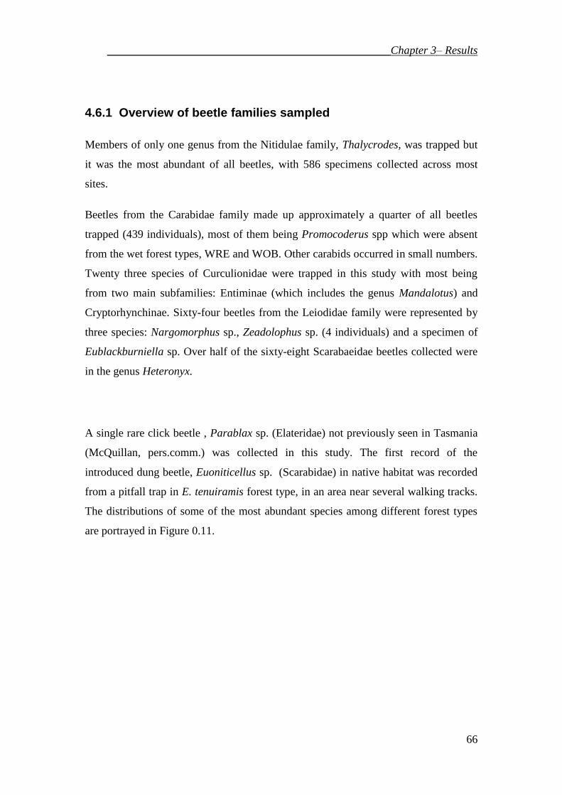
__________________________________________________Chapter 3– Results
66
4.6.1 Overview of beetle families sampled
Members of only one genus from the Nitidulae family, Thalycrodes, was trapped but
it was the most abundant of all beetles, with 586 specimens collected across most
sites.
Beetles from the Carabidae family made up approximately a quarter of all beetles
trapped (439 individuals), most of them being Promocoderus spp which were absent
from the wet forest types, WRE and WOB. Other carabids occurred in small numbers.
Twenty three species of Curculionidae were trapped in this study with most being
from two main subfamilies: Entiminae (which includes the genus Mandalotus) and
Cryptorhynchinae. Sixty-four beetles from the Leiodidae family were represented by
three species: Nargomorphus sp., Zeadolophus sp. (4 individuals) and a specimen of
Eublackburniella sp. Over half of the sixty-eight Scarabaeidae beetles collected were
in the genus Heteronyx.
A single rare click beetle , Parablax sp. (Elateridae) not previously seen in Tasmania
(McQuillan, pers.comm.) was collected in this study. The first record of the
introduced dung beetle, Euoniticellus sp. (Scarabidae) in native habitat was recorded
from a pitfall trap in E. tenuiramis forest type, in an area near several walking tracks.
The distributions of some of the most abundant species among different forest types
are portrayed in Figure 0.11.

__________________________________________________Chapter 3– Results
67
Thalycrodes australe
0
20
40
60
80
WRE WOB DOB DTO DPU DAM
Forest type
Me
an
ab
un
da
nc
e
(a) Thalycrodes australe (Nitidulae)
Promecoderus spp
0
10
20
30
40
50
WRE WOB DOB DTO DPU DAMForest type
Me
an
ab
un
da
nc
e
(b) Promecoderus spp. (Carabidae)
Lissotes spp.
0
0.5
1
1.5
WRE WOB DOB DTO DPU DAM
Forest type
Mean
ab
un
dan
ce
Lissotes forcipula Lissotes obtusatus
(c) Lissotes forcipula and L. obtusatus (Lucanidae)
Pachyporopterus satyrus
0
1
2
3
4
5
6
WRE WOB DOB DTO DPU DAMForest type
Me
an
ab
un
da
nc
e
(d) Pachyporopterus satyrus (Curculionidae)
Mandalotus NM1
0
1
2
3
WRE WOB DOB DTO DPU DAMForest type
Meaan
ab
un
dan
ce
(e) Mandalotus NM1 (Curculionoidae)
)
Figure 0.11 Graphs of mean abundance of common beetle species in different forest types.

__________________________________________________Chapter 3– Results
68
4.6.1 Seasonal variation in distribution of beetles
Seasonal variation in occurrence of species was provided to assess interpretations of
species presence and abundance from sampling of extensive sites in only one season.
Seasonal abundance of beetles in different forest
types
0
20
40
60
80
100
120
140
160
180
WRE WOB DOB DPU DAM DTO
Forest types
Beetl
e a
bu
nd
an
ce
NOV
FEB
APR
Figure 3.12 Seasonal abundance of beetles in different forest types from the Mt Wellington study.
Seasonal occurrence of beetles in the Mt Wellington foothills showed highest
numbers in summer (February) in the wetter WRE and WOB forest types and DOB,
with much lower numbers in autumn (April). There was little seasonal variation in
DPU, while the dry DAM and DTO had slightly lower numbers in summer (February)
than in other months.

__________________________________________________Chapter 3– Results
69
Seasonal abundance of Thalycrodes spp.
0
10
20
30
40
50
60
s1 s2 s3 s4 s5 s7 s12 s16 s6 s17 s8 s20 s13 s18 s11 s24 s14 s15 s22 s23 s9 s10 s19 s21
WRE WOB DOB DPU DAM DTO
Sites grouped by Forest type
Ab
un
dan
ce
Nov
Feb
Apr
(a) Thalycrodes australe spp.
Seasonal abundance of Promecoderus
0
5
10
15
20
25
30
35
40
45
50
s1 s2 s3 s4 s5 s7 s12 s16 s6 s17 s8 s20 s13 s18 s11 s24 s14 s15 s22 s23 s9 s10 s19 s21
WRE WOB DOB DPU DAM DTO
Sites grouped by forest type
Ab
un
dan
ce
Nov
Feb
Apr
(b) Promecoderus sp.
Seasonal abundance of Poropterus sp.
0
2
4
6
8
10
12
14
s1 s2 s3 s4 s5 s7 s12 s16 s6 s17 s8 s20 s13 s18 s11 s24 s14 s15 s22 s23 s9 s10 s19 s21
WRE WOB DOB DPU DAM DTO
Sites grouped by Forest type
Ab
un
dan
ce
Nov
Feb
Apr
(c) Pachyporopterus satyrus
Seasonal abundance of Anotylus
0
2
4
6
8
10
12
14
16
s1 s2 s3 s4 s5 s7 s12 s16 s6 s17 s8 s20 s13 s18 s11 s24 s14 s15 s22 s23 s9 s10 s19 s21
WRE WOB DOB DPU DAM DTO
Sites grouped by Forest type
Ab
un
da
nc
e
Nov
Feb
Apr
(d) Anotylus spp.
Seasonal abundance of Nargomorphus spp.
0
5
10
15
20
25
30
s1 s2 s3 s4 s5 s7 s12 s16 s6 s17 s8 s20 s13 s18 s11 s24 s14 s15 s22 s23 s9 s10 s19 s21
WRE WOB DOB DPU DAM DTO
Sites grouped by Forest type
Ab
un
dan
ce
Nov
Feb
Apr
(e) Nargomorphus spp.
Seasonal abundance of Onthophagus fuliginosus
0
1
2
3
s1
WRE
s3 s5
WOB
s12 s6
DOB
s8 s13
DPU
s11 s14
DAM
s22 s9
DTO
s19
Sites grouped by Forest type
Ab
un
dan
ce
Nov
Feb
Apr
(f) Onthophagus fuliginosus F
igure 3.13 Seasonal occurrence of some of the sampled Mt Wellington beetles in different forest
types in February, April and November.
Beetles varied seasonally in their abundances in different forest type (Figure 3.13).
Thalycrodes australe (Germar, 1848) was generally present across all forest types but
was particularly numerous in WRE and DOB in February. Promecoderus was

__________________________________________________Chapter 3– Results
70
generally found in drier forest types with peak abundances in April. Pachyporopterus
satyrus (Pascoe, 1872) was generally present across all forest types but its peak
abundances occurred in April in DPU and DAM. Onthophagus fuliginosus Erichson,
1842 was absent from wet forest types and absent in November samples. In contrast,
Nargomorphus spp. were confined to wetter sites with peak abundances in November.
Aridius minor (Blackburn, 1888) and Mandalotus NM3 were absent from DPU with
Aridius minor (Blackburn, 1888) showing a peak abundance at a single site in
November and Mandalotus NM3 with higher abundances in November and February
than in April.
4.6.1 Trophic levels of beetles
Mean abundance
Forest Pred st. error Herb st. error Xylo st. error Fung st. error
WRE 9 0.912 4.75 2.174 6 1.414 66 6.164
WOB 15 7.011 5 1.080 6.5 1.707 21.75 4.767
DOB 12.5 6.885 5 1.224 10.5 0.645 60.75 23.23
DTO 44.5 12.92 2.75 1.181 7 2.798 27 6.757
DPU 30 13.97 12 7.153 5.75 1.314 11.25 1.796
DAM 48 12.41 1.75 0.853 4.75 1.314 10.25 2.25
Mean species richness
Forest Pred st. error Herb st. error Xylo st. error Fung st. error
WRE 7.25 0.629 3.5 1.040 4.25 0.629 10.75 1.030
WOB 6 1.732 3.25 0.478 3.25 0.75 7.25 1.25
DOB 5.25 1.931 4.25 0.946 5.25 0.629 4.5 0.288
DTO 5.25 1.25 2.5 1.190 3.25 0.478 4.75 1.652
DPU 4.75 1.108 3.5 0.957 3.25 0.629 3.75 0.478
DAM 3.75 0.853 1.25 0.629 2.25 0.478 3 1.080
Table 3.7 Mean abundance and mean species richness of beetles grouped by trophic level in

__________________________________________________Chapter 3– Results
71
different forest types. Pred = predator, Herb = herbivore, Xylo = xylophage and Fung =
fungivores and saprophages.
Mean abundance of species grouped by
trophic level
0
10
20
30
40
50
60
70
80
90
WRE WOB DOB DTO DPU DAM
Forest type
Mean
ab
un
dan
ce
Pred Herb Xylo Fung
(a)
Mean species richness of trophic levels of
beetles
0
2
4
6
8
10
12
14
WRE WOB DOB DTO DPU DAM
Forest typeM
ean
sp
ecie
s r
ich
ness
Pred Herb Xylo Fung
(b)
Figure 3.14 (a) Mean abundance of beetle species grouped by trophic level. (b) Mean species
richness of beetles grouped by trophic level. Pred = predator, Herb = herbivore, Xylo =
xylophage and Fung = fungivores and saprophages.
Fungivorous beetles outnumbered predators in wet forest types and DOB while
predators were the most numerous in dry forests DTO, DAM and DPU (Figure 3.14
a). Fungivores were more species rich in wet forest types while predators were
slightly more species rich in dry forest types (Figure 3.14 b).
4.1 Spider assemblages
4.7.1 Dominant spider families sampled
A total of 1983 adult and juvenile spiders representing 204 species from 20 families
were sampled at the Mt Wellington sites. Adult spiders alone totalled 1302 individuals
representing 187 species/morphospecies from the same 20 families. The additional

__________________________________________________Chapter 3– Results
72
17 families created from inclusion of juveniles is a possible source of error due to
incorrect identification when calculating diversity. Each of those extra families was
only represented by an abundance of one or two individuals and was excluded from
analyses where rare species (represented by less than five individuals) are first
excluded. The families in the Mt Wellington data that included morphospecies of
only juveniles were Clubionidae and Theridiidae with one extra species, Salticidae,
Thomisidae, Gnaphosidae, Zodariidae and Zoridae with 2 extra species and
Linyphiidae with 5 extra species.
The dominant spider family in terms of abundance was the web builder, Linyphiidae
with 315 individuals from 28 species. The next six dominant families were vagrant
hunters: Lycosidae, Corrinidae, Gnaphosidae, Amaurobiidae, Zoridae, and Zodariidae
(Table 3.8).
Spiders (adults)
Rank Family # individuals
# species
1 LINYPHYIDAE 315 28
2 LYCOSIDAE 300 13
3 CORRINIDAE 255 5
4 GNAPHOSIDAE 182 30
5 AMAUROBIIDAE 138 17
6 ZORIDAE 88 10
7 ZODARIIDAE 70 21
8 THERIDIIDAE 33 11
9 SALTICIDAE 24 18
10 SEGESTRIIDAE 21 2
11 MICROPHOLCOMMATIDAE 13 4
12 NICODAEMIDAE 13 3
13 MYGALOMORPHIDAE 9 4
14 CLUBIONIDAE 4 1
15 MIMMETIDAE 3 3
16 THOMISIDAE 2 4
17 ANAPIDAE 1 3
18 CTENIDAE 1 2
19 GNAPHOSOIDIAE 1 1
20 HAHNIIDAE 1 2
Table 3.8 Ranked order of abundance of adult spider families, including species richness of each
family.

__________________________________________________Chapter 3– Results
73
A list of species/ morphospecies of spiders appears in Appendix 4.
Ranked abundance of adult spiders by family
0
50
100
150
200
250
300
350LIN
YP
H
LY
CO
S
CO
RR
IN
GN
AP
H
AM
AU
R
ZO
RID
ZO
DA
R
TH
ER
ID
SA
LT
IC
SE
GE
S
MIC
RO
PH
NIC
OD
MY
GA
LO
CLU
BI
MIM
ME
T
TH
OM
IS
AN
AP
I
CT
EN
I
GN
AP
HO
SO
ID
HA
HN
I
Family
Ab
un
dan
ce
Figure 3.15 Graphed rank abundance of adult spider families
Spiders (Adults) Species Ranked
Family code Abundance
% of all spiders
Hunting style
Corrinidae SUPPNM1 217 17 vagrant
Linyphiidae LINYDICR 193 15 web
Lycosidae LYCART1 142 11 vagrant
Linyphiidae LINYDIP1 58 4 web
Zoridae ZORHESA 37 3 vagrant
Gnaphosidae GNAPNM16 22 2 vagrant
Linyphiidae LINYNM19 21 2 web
Zodariidae ZODNM12 18 1 vagrant
Gnaphosidae GNAPNM23 17 1 vagrant
Linyphiidae LINYLAE1 17 1 web
Micropholcommatidae MICNM1 16 1 web
Amaurobiidae AMAUNM2 15 1 web
Gnaphosidae GNAPNM15 15 1 vagrant
Gnaphosidae GNAPNM36 15 1 vagrant
Gnaphosidae GNAPNM1 14 1 vagrant
Gnaphosidae GNALNM28 14 1 vagrant
Zodariidae ZODSTFL 14 1 vagrant
Zoridae ZORNM4 13 1 vagrant
Amaurobiidae AMAUNM6 12 1 web
Segestriidae SEGARIAD 12 1 vagrant
Gnaphosidae GNAPNM22 11 1 vagrant
Zodariidae ZODNM25 11 1 vagrant
Gnaphosidae GNAPNM2 10 1 vagrant
Theridiidae THERDIP1 10 1 web
Amaurobiidae AMAUNM8 9 1 web
Lycosidae LYCART6 9 1 vagrant
Theridiidae THERACH 9 1 web

__________________________________________________Chapter 3– Results
74
Gnaphosidae GNAPNM13 8 1 vagrant
Gnaphosidae GNAPNM17 8 1 vagrant
Amaurobiidae AMAUNM3 7 1 web
Gnaphosidae GNAPNM3 7 1 vagrant
Lycosidae LYCVENPI 7 1 vagrant
Lycosidae LYCNM1 7 1 vagrant
Salticidae SALTNM4 7 1 vagrant
Mygalomorphae MYGATRA 7 1 vagrant
Gnaphosidae GNAPNM4 6 <1 vagrant
Linyphiidae LINYLIN1 6 <1 web
Lycosidae LYCTROC2 6 <1 vagrant
Nicodaemidae NICNOVNO 6 <1 web
Gnaphosidae GNAPNM14 5 <1 vagrant
Lycosidae LYCART5 5 <1 vagrant
Lycosidae LYCART8 5 <1 vagrant
Micropholcommatidae MICLONG 5 <1 web
Micropholcommatidae MICTEXN1 5 <1 web
Amaurobiidae AMAUNM1 4 <1 web
Table 3.9 Ranked abundance of spider species sampled with abundance > 4 at Mt Wellington.
Table 3.9 ranks spider species sampled at Mt Wellington. A further 142 species with
abundance less than 5 across all sites have been excluded. The abundances of the
dominant 35 species are displayed in Figure 3.16.
Ranked spider species abundance
0
50
100
150
200
250
SU
PP
NM
1
LIN
YD
ICR
LY
CA
RT1
LIN
YD
IP1
ZO
RH
ES
A
GN
AP
NM
16
LIN
YN
M19
ZO
DN
M12
GN
AP
NM
23
LIN
YL
AE
1
MIC
NM
1
AM
AU
NM
2
GN
AP
NM
15
GN
AP
NM
36
GN
AP
NM
1
GN
ALN
M28
ZO
DS
TF
L
ZO
RN
M4
AM
AU
NM
6
SE
GA
RIA
D
GN
AP
NM
22
ZO
DN
M25
GN
AP
NM
2
TH
ER
DIP
1
AM
AU
NM
8
LY
CA
RT6
TH
ER
AC
H
GN
AP
NM
13
GN
AP
NM
17
AM
AU
NM
3
GN
AP
NM
3
LY
CV
EN
PI
LY
CN
M1
SA
LT
NM
4
MY
GA
TR
A
Species
Ab
un
dan
ce
Figure 3.16 Graph of ranked abundance of the dominant 35 spider species sampled at Mt
Wellington sites.
4.7.1 Seasonal variation in distribution of spiders

__________________________________________________Chapter 3– Results
75
The number of spiders and the number of active species varied seasonally (Figure
3.17).
In drier forests (DOB, DTO, DPU and DAM), species abundance was highest in
November, whereas in wetter forests (WRE and WOB) seasonal abundances were
lower, with a general trend for slightly more spiders in February than November. This
pattern was similar for species richness.

__________________________________________________Chapter 3– Results
76
Seasonal mean abundance of adult spiders
0
10
20
30
40
50
60
70
WRE WOB DOB DTO DPU DAM
Forest type
Mea
n a
bu
nd
an
ce
Feb Apr Nov
(a)
Seasonal mean species richness of adult
spiders
0
2
4
6
8
10
12
14
16
WRE WOB DOB DTO DPU DAM
Forest type
Me
as
sp
ec
ies r
ich
ne
ss
Feb Apr Nov
(b)
Seasonal mean abundance adult and
juvenile spiders
0
10
20
30
40
50
60
70
80
90
WRE WOB DOB DTO DPU DAM
Forest type
Me
an
ab
un
da
nce
Feb Apr Nov
(c)
Seasonal mean species richness of
adult and juvenile spiders
0
5
10
15
20
WRE WOB DOB DTO DPU DAM
Forest type
Mean
sp
ecie
s
rich
ness
Feb Apr Nov
(d)
Seasonal mean abundance of juvenile spiders
0
5
10
15
20
25
30
WRE WOB DOB DTO DPU DAM
Forest type
Mean
ab
un
dan
ce
Feb Apr Nov
(e)
Seasonal mean species richness of juvenile
spiders
0
2
4
6
8
10
12
14
16
WRE WOB DOB DTO DPU DAM
Forest type
Mean
sp
ecie
s r
ich
ness
Feb Apr Nov
(f)
Figure 3.17 Seasonal abundance and species richness of adult and juvenile spiders in different
forest types.
Figure 3.18 provides some typical examples of the seasonal distribution of spider
species in different forest types. Generally species were present at dry forest sites or
wet forest sites, but all showed a large variation within each forest type, as
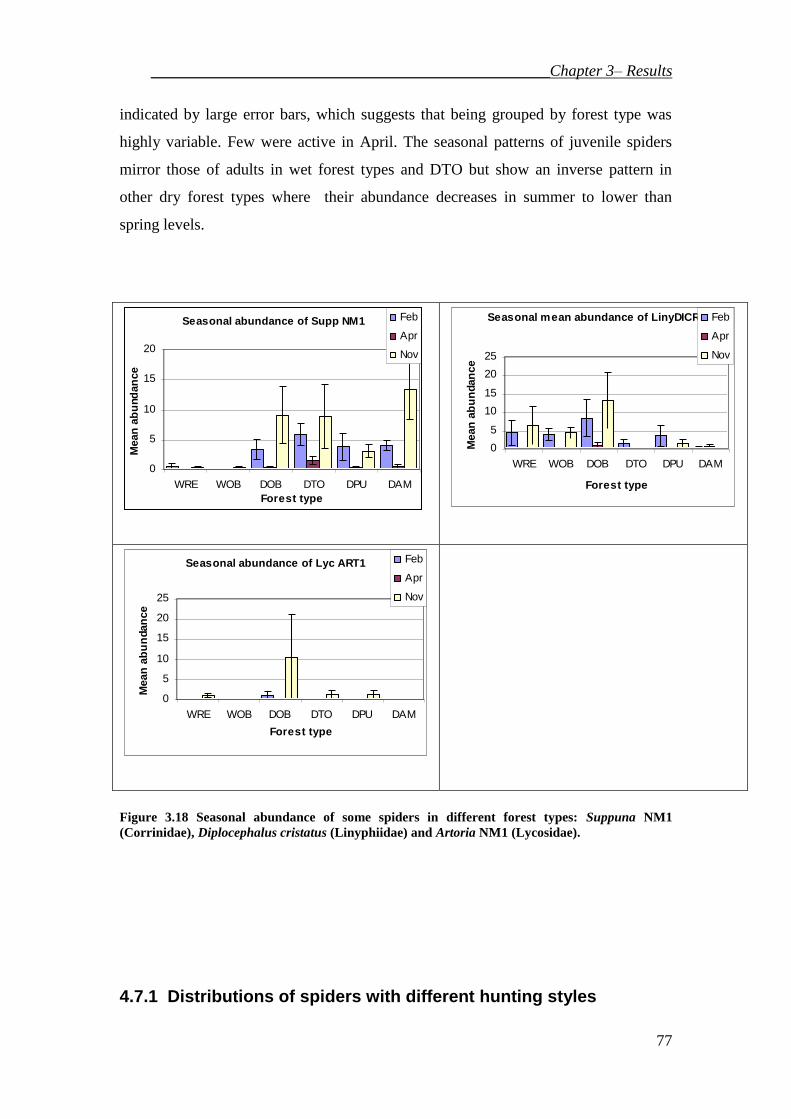
__________________________________________________Chapter 3– Results
77
indicated by large error bars, which suggests that being grouped by forest type was
highly variable. Few were active in April. The seasonal patterns of juvenile spiders
mirror those of adults in wet forest types and DTO but show an inverse pattern in
other dry forest types where their abundance decreases in summer to lower than
spring levels.
Seasonal abundance of Supp NM1
0
5
10
15
20
WRE WOB DOB DTO DPU DAM
Forest type
Mean
ab
und
an
ce
Feb
Apr
Nov
Seasonal mean abundance of LinyDICR
0
5
10
15
20
25
WRE WOB DOB DTO DPU DAM
Forest type
Mean
ab
un
dan
ce
Feb
Apr
Nov
Seasonal abundance of Lyc ART1
0
5
10
15
20
25
WRE WOB DOB DTO DPU DAM
Forest type
Mean
ab
un
dan
ce
Feb
Apr
Nov
Figure 3.18 Seasonal abundance of some spiders in different forest types: Suppuna NM1
(Corrinidae), Diplocephalus cristatus (Linyphiidae) and Artoria NM1 (Lycosidae).
4.7.1 Distributions of spiders with different hunting styles

__________________________________________________Chapter 3– Results
78
Distribution of web builders and vagrant
hunters
0
20
40
60
80
100
120
WRE WOB DOB DTO DPU DAM
Forest type
Mean
ab
un
dan
ce
Web
Vagr
(a)
Species richness of web builders and
vagrant hunters
0
5
10
15
20
25
WRE WOB DOB DTO DPU DAM
Forest type
Me
an
sp
ec
ies
ric
hn
es
s
Web
Vagr
(b)
Figure 3.19 Mean abundance (a), and species richness (b), of web builders and vagrant hunters in
different forest types.
Web building dominated the numbers and species richness of spiders in wet forest
types. Vagrant hunters were dominant in abundance and species richness in the drier
forest types (Figure 3.19).
4.1 Statistical Analysis of data
4.8.1 Beta diversity
Species abundance and richness varied between forest types (Figure 3.20).

__________________________________________________Chapter 3– Results
79
Abundance of beetles and
spiders
0
20
40
60
80
100
120
140
160
WRE WOB DOB DTO DPU DAMForest type
Mean
ab
un
da
nce
beet les
spiders
Species richness of beetles
and spiders
0
5
10
15
20
25
30
35
40
WREWOB DOB DTO DPU DAMForest type
Mean
sp
ecie
s
rich
ness
beet les
spiders
Figure 3.20 Comparison of beetle and spider abundance and species richness in different forest
types.
Dry forest types (WOB, DTO, DPU and DAM) contained more spiders than beetles
and a greater diversity of spiders. The opposite was observed in wet forests (WRE and
WOB) where beetles dominated spiders in diversity and abundance.
4.8.1.1 Local variation
Local variation in beta diversity for different taxa among adjacent forest types is
compared in Table 3.10 using a modified Whittaker’s index for beta diversity
(Harrison et al. 1992).
Spp Rich-
ness
diversity indices overal
l
Forest type
WRE WOB DOB DTO DPU DAM
Modified Vascular
plants 147 22.83
18.26 7.43 12.53 7.52 8.19 7.43
Whittaker’s Beetles 152 24.48 22.79 26.43 28.73 38.87 50.84 24.48
Index Spiders
(all) 204 34.11 36.96 28.61 24.64 28.61 31.68 28.61
Spiders
(adults) 187 45.17 45.17 28.04 29.04 31.27 35.35 29.04
Fungi 64 23.19 14.65 27.83 46.38 139.13 69.57 14.65
Table 3.10 Whittaker’s Index for beta diversity, modified by Harrison et al. (1992) for the Mt
Wellington species. Sampling occurred in February, April and November.

__________________________________________________Chapter 3– Results
80
The degree to which sites in one forest type shares species with sites in another forest
type is referred to as species turnover (Oliver et al. 1998). Species turnover was
lower (more species in common) for vascular plants than invertebrates, indicating that
sites within the same forest types generally shared the same plant species. The drier
forest types (DOB, DTO, DPU and DAM) had the lowest plant species turnover (beta
diversity lowest in DOB and DPU at 7.43 and 7.52 respectively). Conversely, beetles
had highest species turnover between sites within two of the drier forest types (DPU
and DAM with beta diversity 38.87 and 50.84 respectively). Adult spiders showed
highest species turnover among wet forest types (WRE and WOB with beta diversity
45.17 for each). Fungi demonstrated exceptionally high species turnover among drier
forest types.
It should be noted, that unlike plants, repeated sampling for fungi will continue to
reveal new species with different species occurring in different years as well as
seasons (Sapphire McMullan-Fisher, pers. comm.) Thus the single sampling for fungi
in this study did not necessarily provide a representative measure of fungal beta
diversity from which comparisons with other taxa could be made.
When beta diversity of the whole study area (1.3 km2) was considered, regardless of
forest types contained within it, vascular plants had the lowest diversity (7.43) ,
followed by fungi with a beta diversity of 14.65. The turnover of beetles and spiders
was higher than for plants with a beta diversity of 24.45 for beetles and 29.04 for
adult spiders.
4.8.1.2 Regional variation
At the regional scale beta diversity indices were calculated for each forest type within

__________________________________________________Chapter 3– Results
81
each region as well as for each region regardless of forest type (Table 3.11).
SPECIES
Spp
Rich diversity indices
REGION *
REGION
Hobart | Levendale | Swansea Hob Lev. Swa.
DOB DPU DOB DPU DOB DPU
Modified Beetles 186 29.52 26.57 21.56 18.98 32.11 27.97 18.98 40.00 36.04 35.18
Whittaker’s Spiders (all) 196 29.47 25.45 29.47 15.56 31.11 20.74 15.56 38.43 28.03 29.29
Index Spiders
(adults) 182 34.67 30.59 28.89 16.77 32.50 22.61 16.77 41.71 30.21 30.85
Table 3.11 Table of Whittaker’s B-diversity index modified by Harrison et al, (1992), for the
regional species. Sampling occurred in November. (*= for all three regions combined).
Within each region beta diversity was higher in DOB forest type than DPU. This was
the opposite of the trend for Mt Wellington, however the Mt Wellington samples
contained species present in April and February and November whereas regional scale
sampling only occurred in November.
Overall beta diversity of each region was similar for beetles and spiders, with the
index ranging from 16 to 19.
4.8.1 Do assemblages of beetles and spiders correspond to
mapped forest types?
4.8.1 Non-parametric MANOVA
Non-parametric MANOVA (NP-MANOVA) was used to analyse species occurrence
across sites in the foothills of Mt Wellington. It provided a test for whether species
from the same forest type group were more similar than species from other forest type
groups. The output below is from a one-way ANOVA design consisting of sites
(samples) grouped within 6 different forest types (factors) with 4 replicates of each.
Data were fourth root transformed and distances between pairs of samples were
calculated using the Bray-Curtis dissimilarity measure which is appropriate for zero-
inflated data. Results are based on 4999 permutations. Pair-wise a posteriori tests

__________________________________________________Chapter 3– Results
82
were performed on the six forest types.
Non-parametric Multivariate Analysis of Variance
Variables Source df SS MS F P
Beetles Forest 5 23696.8750 4739.3750 2.1242 0.0002
152 spp Residual 18 40160.2199 2231.1233
Total 23 63857.0949
Spiders Forest 5 24452.3260 4890.4652 2.0497 0.0002
(adults) Residual 18 42947.6129 2385.9785
187 spp Total 23 67399.9390
Table 3.12 Results of one-way anovas for species occurrences in different forest types.
NP MANOVA Tests among groups in factor 'forest'
Beetles
Spiders
(adults)
Groups t P Groups t P
( WRE, WOB) 1.1165 0.2298 ( WRE, WOB) 1.4635 0.0294
( WRE, DOB) 1.349 0.0308 ( WRE, DOB) 1.2724 0.0564
( WRE, DTO) 2.0596 0.0292 ( WRE, DTO) 1.8556 0.0292
( WRE, DPU) 1.4294 0.0282 ( WRE, DPU) 1.5386 0.0282
( WRE, DAM) 2.1843 0.0316 ( WRE, DAM) 2.0254 0.0316
( WOB, DOB) 1.1824 0.115 ( WOB, DOB) 1.3061 0.0262
( WOB, DTO) 1.8658 0.0298 ( WOB, DTO) 1.6534 0.0298
( WOB, DPU) 1.1474 0.2128 ( WOB, DPU) 1.4408 0.0302
( WOB,DAM) 1.8976 0.0276 ( WOB, DAM) 1.7384 0.0276
( DOB, DTO) 1.4201 0.0262 ( DOB, DTO) 1.1224 0.1462
( DOB, DPU) 1.0121 0.4938 ( DOB, DPU) 1.0273 0.3878
( DOB, DAM) 1.5742 0.0316 ( DOB, DAM) 1.1082 0.2612
( DTO, DPU) 1.0649 0.2816 ( DTO, DPU) 1.2435 0.0824
( DTO, DAM) 1.1034 0.1882 ( DTO, DAM) 0.9892 0.5432
( DPU, DAM) 1.1544 0.253 ( DPU, DAM) 1.4062 0.057
Table 3.13 Pairwise a posteriori comparisons of dissimilarity in assemblages between groups of
forest type. Significant pairwise differences between forest types appear in bold type (at p < 0.05
level of significance).
Examination of NP-MANOVA results for beetles (Table 3.12) indicates that overall

__________________________________________________Chapter 3– Results
83
there was a significant difference in occurrence of beetles in different forest types
(p=0.0002). However, pair-wise a posteriori comparisons of forest types (Table 3.13)
indicates that the differences in occurrence were not significant for all forest types.
Beetle assemblages in wet WRE were significantly dissimilar to beetle assemblages in
all dry forest types (p < 0.032). Beetle assemblages in DTO were not significantly
different to DAM, and assemblages in WOB were not significantly different to those
in DOB. Beetle assemblages in the wet and dry E. obliqua forest sites (WOB and
DOB) were, however, significantly different to DAM (p= 0.0276 and p= 0.0316
respectively) and DTO (p= 0.0298 and p= 0.0262 respectively).
For spiders there was a consistent dissimilarity in spider assemblages in wetter forest
types compared to those in drier forest types. WOB was dissimilar to all other forest
types including the other wet type, WRE, suggesting that factors other than moisture
might be relevant. WRE was significantly dissimilar to all other forest types except
DOB which was nearly significantly different (p = 0.0564). Where there was an
insignificant difference between pairs of forest types then species distribution may be
a response to factors other than forest type or due to high variation.
Dispersion of the spider and beetle data was tested before the significant of the NP-
MANOVA could be interpreted as showing that invertebrates from the same forest
type were more similar than assemblages from different sites. Dispersion was
different in each case (Figure 3.14).
Variables Source df SS MS F P
Beetles Forest 5 517.494 103.4989 3.5514 0.0244
152 spp Residual 18 524.5789 29.1433
Total 23 1042.0734
Spiders Forest 5 126.6726 25.3345 0.8502 0.5271
(adults) Residual 18 536.3523 29.7973
190 spp Total 23 663.0249
Table 3.14 Permutational Test of Multivariate Dispersion: tests for heterogeneity in the average
dissimilarities of points from the central location of their group.
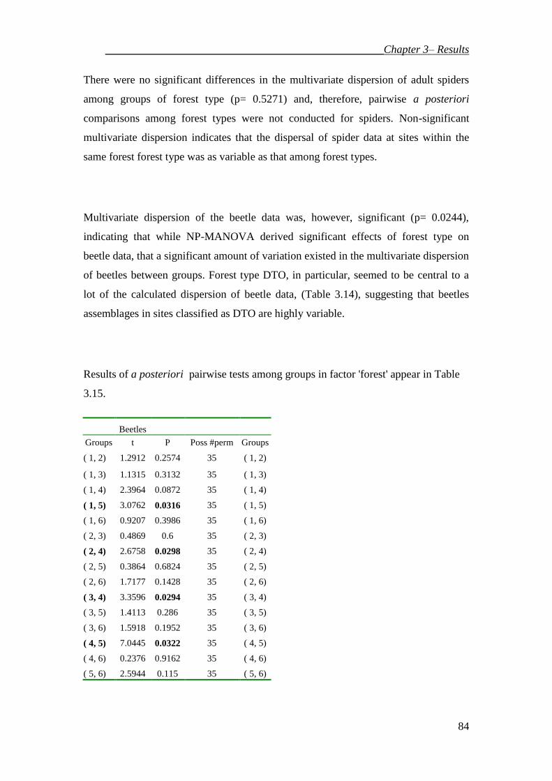
__________________________________________________Chapter 3– Results
84
There were no significant differences in the multivariate dispersion of adult spiders
among groups of forest type (p= 0.5271) and, therefore, pairwise a posteriori
comparisons among forest types were not conducted for spiders. Non-significant
multivariate dispersion indicates that the dispersal of spider data at sites within the
same forest forest type was as variable as that among forest types.
Multivariate dispersion of the beetle data was, however, significant (p= 0.0244),
indicating that while NP-MANOVA derived significant effects of forest type on
beetle data, that a significant amount of variation existed in the multivariate dispersion
of beetles between groups. Forest type DTO, in particular, seemed to be central to a
lot of the calculated dispersion of beetle data, (Table 3.14), suggesting that beetles
assemblages in sites classified as DTO are highly variable.
Results of a posteriori pairwise tests among groups in factor 'forest' appear in Table
3.15.
Beetles
Groups t P Poss #perm Groups
( 1, 2) 1.2912 0.2574 35 ( 1, 2)
( 1, 3) 1.1315 0.3132 35 ( 1, 3)
( 1, 4) 2.3964 0.0872 35 ( 1, 4)
( 1, 5) 3.0762 0.0316 35 ( 1, 5)
( 1, 6) 0.9207 0.3986 35 ( 1, 6)
( 2, 3) 0.4869 0.6 35 ( 2, 3)
( 2, 4) 2.6758 0.0298 35 ( 2, 4)
( 2, 5) 0.3864 0.6824 35 ( 2, 5)
( 2, 6) 1.7177 0.1428 35 ( 2, 6)
( 3, 4) 3.3596 0.0294 35 ( 3, 4)
( 3, 5) 1.4113 0.286 35 ( 3, 5)
( 3, 6) 1.5918 0.1952 35 ( 3, 6)
( 4, 5) 7.0445 0.0322 35 ( 4, 5)
( 4, 6) 0.2376 0.9162 35 ( 4, 6)
( 5, 6) 2.5944 0.115 35 ( 5, 6)

__________________________________________________Chapter 3– Results
85
Table 3.15 Pair-wise a posteriori comparisons of beetle assemblages among forest types.
Average within-group dissimilarities
Beetles WRE 64.090
WOB 73.290
DOB 69.475
DTE 55.635
DPU 75.537
DAM 57.425
Spiders (adult) WRE 60.581
WOB 71.107
DOB 72.161
DTE 70.081
DPU 67.817
DAM 69.404
Table 3.16 Average within group dissimilarity for beetles and spiders
Average dissimilarities within/between groups
Beetles 1 2 3 4 5 6
1 64.090
2 70.876 73.290
3 73.219 75.043 69.475
4 80.845 83.007 70.235 55.635
5 78.784 77.163 72.792 67.057 75.537
6 85.643 85.209 74.847 58.169 69.463 57.425
Spiders
(adult)
1 2 3 4 5 6
1 60.581
2 74.485 71.107
3 71.601 77.357 72.161
4 83.317 84.524 73.752 70.081
5 74.492 78.169 70.842 73.913 67.817
6 87.206 86.407 73.100 69.768 77.025 69.404
Table 3.17 Matrices of Bray-Curtis dissimilarities within and between groups.
Matrices of Bray-Curtis dissimilarity indices within and between groups, (Figure
3.17), indicate that the dissimilarity between assemblages of species at sites with the
same forest type (the diagonal of each matrix) are almost as high as the dissimilarity
between assemblages in different forest types. This trend is more pronounced for the

__________________________________________________Chapter 3– Results
86
spider assemblages.
MDS ordinations of sites in beetle and in spider species ‘spaces’ provide a visual
representation of the dissimilarity in assemblages between sites just discussed (Figure
3.21).
Since grouping sites by forest type did not provide a clear correspondence to species
assemblages, the variation in species among the sites within each forest type was
examined more closely.
Nonmetric Multidimensional Scaling (NMDS) was appropriate for species data that is
not necessarily normally distributed. Separate ordinations of matrices of beetle,
spider (all), spider (adults), fungi, and vegetation species for each site provided a
visual presentation of Bray-Curtis dissimilarity indices between assemblages at each
site. Abundance data were transformed for beetle and spider abundances to ln(x+1) so
that highly abundant species did not dominate the ordination patterns. Fungi volume
and scored vegetation cover data were not transformed.

__________________________________________________Chapter 3– Results
87
(a)Vegetation ordination: 2-D Stress = 9.1766, 400 iterations
(b) Beetle ordination: 3-D Stress = 11.30037, 63 iterations

__________________________________________________Chapter 3– Results
88
(c) Adult spiders ordination: 2-D Stress =16.7265, 67 iterations
(d) All spiders ordination: 3-D Stress =12.48527, 48 iterations
Figure 0.21 Ordinations of sites in different species spaces. Sites grouped closer together share
more similar species than those spaced further apart. Key to forest types: 1 = WRE, 2= WOB, 3=
DOB, 4 = DAM, 5 = DPU, 6 = DTO.
Sites with similar assemblages may be assessed from the ordinations in Figure 3.21

__________________________________________________Chapter 3– Results
89
where sites with more similar assemblages are grouped closer together and those that
are more dissimilar are spaced further apart.
The ordination of sites in plant species space results in some discrete grouping of sites
that reflect forest type quite well, particularly DTO and DOB. The horizontal
ordination axis shows a degree of mesic separation of sites, with wetter WRE and
WOB to the right and drier types to the left. The two wetter forest type sites are
intermingled in the ordination, suggesting overlap of species, and their loose
clustering implies variation from site to site within the same forest type. Overlap of
vegetation species at sites located in drier forest types DAM and DPU areindicated by
clustering of these sites amongst each other. Less difference in vegetation between
sites resulted in closer clustering of those sites, though site 13 (DPU) has different
species to any others. The vertical ordination axis separates sites separated DTO and
DPU sites from the rest, indicating a difference in vascular plant species in these two
forest types compared with the other types. The stress of 9.17671 for the ordination of
sites by vegetation species suggests that the result is a fairly reliable plot of sites in
relation to their original ranked distances. In this case the plot suggests that forest type
is largely indicated by patterns in distribution of vegetation species.
The ordination of sites in beetle and spider species spaces resulted in loose clustering
of sites in similar forest type dominated by overlap between the forest types. Sites
from quite different forest types were more closely clustered due to higher similarity
in beetle species. This suggests that factors other than forest type may be influencing
distribution of beetle and species. The ordination enables a preliminary investigation
of spatial autocorrelation by referring to the map (Figure 2.1), where sites from
different forest types that have clustered together due to similarity in beetle
assemblages are not in adjacent patches. For example the pair of sites 21(DTO) and
23 (DAM) show a strong similarity in assemblages but are further separated by
patches of DPU and DOB. Sites 3 (WRE), 19 (DTO) and 20 (WOB) have many
species in common, despite other intervening forest types. In contrast, sites 8 and 20
are near each other in the same patch of DOB and are widely separated in the
ordination due to few shared species. A more robust test for autocorrelation will be

__________________________________________________Chapter 3– Results
90
conducted in a later section. The ordination 3-D stress value of 11.3 indicates that
some caution should be exercised in interpreting this plot, and finer details should be
disregarded as it cannot be reliably interpreted (McCune and Grace, 2002). However,
the poor relationship between forest type and beetle assemblage is loosely
demonstrated by the ordination.
The horizontal axis separated mesic forest sites when ordinated by adult spiders and
by all spiders but sites of the same forest type were still widely dispersed, suggesting
that this factor alone was not enough to account for differences between sites. No
pattern was discernable for separation of sites along the vertical axis. A stress of
16.7265 for the 2-D ordination of adult spiders and 12.4527 for a 3-D ordination of
all spiders meant that there is some unreliability in the ordinations so caution should
be exercised when interpreting them.
4.8.1 ANOSIM
A more rigorous test of these differences in assemblages grouped by forest type was
pursued with an Analysis of Similarity (ANOSIM) which was suited to the one-way
design of this study. The analysis, conducted in R, is a non-parametric permutation of
dissimilarity ranks from a Bray-Curtis matrix of dissimilarity between pairs of sites to
test for a significant difference in the composition of assemblages at different sites.
The number of permutations was 10,000.
Beetle community similarity with forest type Spider (all) community similarity with forest

__________________________________________________Chapter 3– Results
91
type
Fungi community similarity with forest type Spider (adult) community similarity with
forest type
Species R p
beetles 0.513 <0.001
spiders (all) 0.3963 <0.001
Spiders
(adults)
0.4166 <0.001
fungi 0.3037 <0.001
(Based on 1000 permutations)
Figure 3.22 The effect of forest type on species communities. Boxplots portray the mean ranks of
dissimilarity between and within groups. Key to forest types: 1 = WRE, 2= WOB, 3= DOB, 4 =
DAM, 5 = DPU, 6 = DTO.
For ANOSIM (Figure 3.22) the R statistic has a range of 1 to -1 with a value of zero if
groups are independent and was significant for all analyses (p < 0.001). Analysis
conducted for similarity of beetle assemblages with forest type showed the strongest
difference in beetle species among different mapped forest types (R = 0.513). The
difference for adult spiders alone (R = 0.41166) was stronger than when all spiders
were analysed (R = 0.3963). Fungi data showed weakest differences between forest
types (R = 0.3037).
The boxplot of beetles shows little variation in beetle species at different sites within
forest type WRE, while there is wide variation between species at different sites
within the same forest type for all other forest types. Adult and all spider species

__________________________________________________Chapter 3– Results
92
varied widely in sites within the same forest type for all forest types, which implies
there was a lower relationship between forest type and spider species.
4.8.1 Do all forest types contribute equally to species variation?
Having investigated whether forest type has an effect on assemblages, a CAP analysis
was able to reveal the amount of variation explained by forest type and which forest
types explained any of that variation.
CAP analysis using discriminant analysis to test for differences among forest types
(groups) in beetles and spiders (adults and juveniles; and adults only) provided the
results in Table 3.18. Cross validation of the canonical correlations using a leave-one-
out permutation test are included. All analyses used fourth root transformed species
data and Bray-Curtis dissimilarity indices.
Effect of
Forest type
on:
m
Variation
explained
(%)
Successful Allocation to Forest Type (%) WRE WOB DOB DTO DPU DAM Total
p
beetles 7 71.435 50 75 25 50 0 75 45.833 0.069088 0.8558
Spiders
(all)
7 64.498 100 75 75 25 0 0 45.833 0.909598 0.0011
Spiders
(adults)
15 92.203 75 75 0 50 50 75 54.167 0.385911 0.3944
Table 3.18 Summary CAP results to determine the effect of forest type on beetle and spider
assemblages at each site. ‘m’ is the number of first principal coordinates selected by the program
during the analysis. ‘Variation explained’ refers to the variation explained by the first m
principal coordinates.
Successful classification of beetles to forest type was highest (75%) for forest types

__________________________________________________Chapter 3– Results
93
WOB and DAM, while there was zero successful allocation to DPU. Assemblages of
beetles in DOB (25% successful allocation) were highly random, and even more
random in DPU but more discrete and distinctive in forest types WOB and DAM.
CAP analysis indicated that forest type was not significant for beetles, with a very low
squared canonical correlation (δ2) of 0.069088 (p= 0.8558).
For all spiders leave-one-out allocation was 100% successful in allocation to forest
type 1 (WRE) but had zero success with forest types DPU and DAM. CAP analysis
indicated that forest type was highly significant for all spiders, with δ2 = 0.909598
(p= 0.0011).
When juvenile spiders were removed from the analysis, allocation was more
consistently successful across each of the forest types apart from total failure to
successfully allocate adult spiders to forest type DOB (0%). The CAP analysis
produced a lower squared canonical correlation (δ2
= 0.385911) than when all spiders
were included, and its value was no longer significant (p= 0.3944) ie forest type was
not significant for adult spiders alone.
CAP output of correlations of canonical axes with original axes generated low
correlations. Examination of the correlations enabled the species more highly
correlated with the canonical axes to be identified. Species most highly correlated
with canonical axes, with a correlation value > 0.6, are listed in Table 3.19. They are
the species contributing most to multivariate distribution of beetles among forest
types.

__________________________________________________Chapter 3– Results
94
Correlation value
Assemblage Species Canonical axis
1 2 3 4 5
Beetles Nemadini sp.: Leiodidae -0.6496
Thalycrodes australis: Nitidulae -0.7076
Acrotrichis sp. : Ptilidae 0.6550
Scaphisoma sp. : Staphylinidae -0.6017
Isopteron obscurum: Tenebrionidae 0.6621
Tetrabothrus claviger: Staphylinidae 0.6381
Spiders Suppuna picta: Corrinidae 0.7654
(all) Gnaphosidae NM34: Gnaphosidae 0.7757
Lycosidae NM1: Lycosidae 0.6321
Micropholcommatidae NM8: Microphol. 0.6129
Zodariidae NM26: Zodariidae 0.6372
Zoridae NM1: Zoridae 0.6176
Spiders Hestimodema A: Zoridae 0.7248
(adults)
Fungi Descolea sp Bolbitaceae
Clavaria miniata complex: Clavariaceae
Geastrum sp. B: Geastraceae
Russula sp. pink: Russulaceae
Stereum sp. C yellow: Stearaceae
Leucopaxillus sp.: Tricholomataceae
-0.714
0.685
0.8685
-0.6303
-0.8733
0.6297
Table 3.19 Highest values for correlation of canonical axes with original axes from CAP analyses
for forest type
The low correlation of most species with the canonical axes is demonstrated by the
plot below where beetle species variation does not correspond to locations of sites
(Figure 3.23).

__________________________________________________Chapter 3– Results
95
Figure 3.23 Canonical correlation of beetle species data plotted for the first two canonical axes.
Crosses indicate species distributions and triangles indicate sites.
4.8.5.1 CAP CCA
A slightly different canonical analysis of principal coordinates, this time under
canonical correlation, provided an indication of the relationship between species
distribution and environmental variables. In this analysis a slightly larger subgroup of
beetles was found to be correlated with canonical axes, though most correlations were
not really strong. The variables were independent of forest type:
The CAP (Anderson, 2004) analysis was by Canonical Correlation Analysis (CCA)
enabling a multivariate eigenanalysis with a permutation test for the relationship
between species distribution and environmental variables.

__________________________________________________Chapter 3– Results
96
Correlation value
Assemblage Species number and name Canonical axis
1 2 3 4 5
Beetles Nemadini: Leiodidae 0.7229
Zeadolopus NM2: Leiodidae 0.6476
Thalycrodes australe: Nitidulae 0.6944
Thalycrodes cylindricum: Nitidulae 0.6858
Scaphisoma sp.: Leiodidae 0.7255
Rybaxis rugosus: Pselaphidae 0.6369
Mandalotus NM1: Curculiuonidae
Anotylus B: Staphylinidae
-0.7734
0.6102
Spiders Suppuna NM1: Corrinidae -0.8022
(all) Gnaphosidae NM1: Gnaphosidae -0.6715
Laetesia NM1: Linyphiidae -
0.6246
Mynogleninae NM33: Linyphiidae
0.6714
Storena flavipes: Zodariidae -0.6545
Zodariidae NM12; Zodariidae -0.6306
Spiders None
(adults)
Fungi Descolea sp. Bolbitiaceae
Geastrum sp. B: Geastraceae
-0.6839
-0.7046
Table 3.20 Highest values for correlation of canonical axes with original axes from CAP analyses
for environmental variables.
The plots of principal component axes and canonical axes (Figure 3.34) represent the
quite variable differences in composition and abundance of beetles species at each site
based on environment variables. Similar variation occurred in the plots for spiders so
they are not reproduced here.

__________________________________________________Chapter 3– Results
97
Principal coordinates plot for beetles Canonical plot for beetles
Figure 3.24 Plots of the first two principal coordinates axes and canonical axes from CAP
analysis for beetles.
Having identified wide variation in assemblages among sites even within the same
forest type, the next phase of the analysis was to identify the environmental variables
that species of beetles and spiders were responding to other than mapped forest type.
4.8.1 Which environmental variables are related to species
distributions?
4.8.6.1 NMDS
All environmental variables were included in NMDS ordinations of species data in
which biplots of environmental data identified variables with the strongest
relationship with species variation. This enabled the number of variables to be
reduced, for further analyses, to those contributing most to variation in species
distributions.

__________________________________________________Chapter 3– Results
98
(a) beetles ( b) spiders
Figure 3.25 NMDS ordination of sites in species space with biplots of the variables contributing
most to the ordination axes., cutoff: r2 = 0.2
The clustering of sites in species space (Figure 3.25) corresponded to two quite
distinct groups for both beetles and spiders. Variation in beetle assemblages caused
vertical separation of sites along a moisture/temperature gradient (Axis 2). Thus
beetles at sites in wetter forest types were associated with higher canopy cover, ferns,
broad leaf shrubs and higher volume of fungi. At the drier end of the gradient beetles
from drier DPU, DAM and DTO were associated with higher summer and winter
radiation and higher litter temp. A further separation of sites along Axis 1 related to
the structure of ground cover, with beetles from wetter sites more closely associated
with greater volume of coarse woody debris, greater depth of the top soil and higher
levels of phosphorus in the top soil (A horizon). The other end of the groundcover
gradient was characterised by the amount of rock in the subsoil (B horizon), shrub
cover of the ground, soil hardness and area of bare ground.
Fewer environmental variables explained the distribution of adult spiders. Axis 2
represented a moisture gradient that separated spiders associated with higher humidity
at ground level, higher soil moisture and broad leaf shrubs, from higher radiation at

__________________________________________________Chapter 3– Results
99
ground level after allowing for canopy cover, higher subsoil temperatures in winter
and higher litter temperature in winter. Axis 1 separated the sites along a gradient of
soil nutrients, with spiders in the wetter sites associated with higher levels of nitrogen
in the top soil (A horizon) and higher minimum levels of nitrogen in the subsoil (B
horizon). Spiders in the drier sites were associated on the soil nutrient gradient with a
higher carbon to nitrogen ratio in the topsoil (A horizon).
For beetles the above results are supported by the variation explained by the principal
coordinates axes resulting from the Cap (CCA) analysis which are presented as a
piechart, Figure 3.26.
(a) Beetles
Figure 3.26 Variation of beetle data explained by Principal coordinates axes from canonical
correlation analysis with environmental data.
4.8.6.2 Regression tree models

__________________________________________________Chapter 3– Results
100
Regression tree models were built in R using the tree package (Ripley, 2007) to
determine which of the numerous environmental variables measured were important
to beetle and spider distribution. Rarer species (abundance less than 5) were removed
from the data (as indicated under each tree) since their occurrence was not significant
enough to detect patterns with environmental variables. All environmental variables
were used.
In the output diagrams (Figure 3.27) the improvement in prediction error obtained by
the split is proportional to the depth of the tree below each split. At each node the
variable that distinguishes best between observations is identified along with the value
at which the split occurs. The leaves of the tree present the mean of species present in
that particular split of the data.
The first set of regression trees below regress site against different multivariate
variables: environmental, beetle abundance, spider abundance and fungi volume.

__________________________________________________Chapter 3– Results
101
(a) Site against environmental variables cut = 3 (b) Site against standardised environmental
variables cut = 6
(c) Site against Beetles (d) Site against Spiders(all)
(e) Site against Spiders (adults) (f) Site against Fungi
Figure 3.27 Regression trees for site regressed against environmental variables with two different
grouping levels (a) cut = 3, and (b) cut = 6, and site against (c) beetles, (d) spiders (all), (e) spiders
(adults), and (f) fungi.

__________________________________________________Chapter 3– Results
102
Regression trees in Figure 3.27 indicated that three variables were valuable predictors
of site difference. At a finer scale (cut =3) (Figure 3.27 a) the variables were litter
temperature, the minimum values of bottom soil carbon content (Soil LBC), and the
highest values of nitrogen in the top soil (Soil HTN). These variables only applied to a
small number of the 24 sites. Most (mean 19.4) had a higher litter temperature >
28.84). For this reason the analysis was repeated with a cut of 6 (Figure 3.27 b). This
produced a grouping of the sites based on canopy cover less than 71% which
corresponded to low subsoil temperatures at a mean of 21 of the sites and low
humidity at a mean of 9.5 of the sites. Generally there was a predictable variation in
sites in relation to environmental variables such that canopy cover (< 0.711705)
corresponded to low subsoil temperature at a mean of 21 sites, but higher subsoil
temperatures corresponded to differences in humidity at sites.
A predictable variation in the sites was also discernable such that the abundance of
Nemadini sp. (<0.9) corresponded to high abundance of Promecoderus sp. at a mean
of 21 sites, and low numbers of Promecoderus sp. (< 3.38) corresponded to
differences in abundances of Mandalotus NM3 at different sites.
The abundance of the spider species Suppuna NM1 provided predictable variation in
sites in relation to spiders. The variation was slightly different for adults only and
adult plus juvenile assemblages. For all spiders (Figure 3.27d) an abundance of
Suppuna NM1 < 1.6 occurred at a mean of 6.8 sites. Suppuna NM1 abundance greater
than 1.6 in fact corresponded to its higher abundance (>3.58) at a mean of 8.5 sites.
Between these two values its abundance corresponded to higher abundance of
Micropholcommatidae NM1 (>1.2) at an average of 9.5 sites. Lower abundances of
Micropholcommatidae corresponded to that of Zodariidae NM12.
With the exclusion of juvenile spiders (Figure 3.27e), the predictable variation in sites
was that higher Suppuna NM1 abundandance (> 0.35) corresponded to a higher

__________________________________________________Chapter 3– Results
103
Amaurobiidae NM2 abundance at an average of 7.75 sites. Lower Amaurobiidae
abundance (< 0.34) corresponded to higher Gnaphosidae NM28 abundance at a mean
of 10.5 sites. Lower Gnaphosiidae NM28 abundance (<1.03) corresponded to a
Supunna NM1 abundance > 3 at a mean of 11.5 sites.
For fungi it was predictable that the occurrence of lower volumes of Descolea spp.
across the sites (<0.14) corresponded to occurrence of Cortinaria C, while Descolea
spp. volumes greater than this further differentiated sites. A volume of Descolea spp.
greater than 3.06 occurred at a mean of 14 sites and a volume between 14 and 3.05
occurred with greater frequency at a mean of 17.5 sites.
4.8.6.3 BIOENV
The Bioenv function sequentially adds a variable to the model and rejects it if that
combination of variables does not improve the fit of the model to the data set. To
ensure that the order in which variables are added did not affect the outcome, the
function was run several times on a dataset with the order of the variables randomly
shuffled manually. In each case the same optimal subsets were selected by the
program.
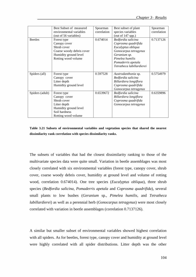
__________________________________________________Chapter 3– Results
104
Best Subset of measured
environmental variables
(out of 56 variables)
Spearman
correlation
Best subset of plant
species variables
(out of 147 spp.)
Spearman
correlation
Beetles Forest type
Canopy cover
Shrub cover
Coarse woody debris cover
Humidity ground level
Rotting wood volume
0.674014 Bedfordia salicina
Coprosma quadrifida
Eucalyptus obliqua
Gonocarpus tetragynus
Geranium sp.
Pimelea humilis
Pomaderris apetala
Tetratheca labillardierei
0.7137126
Spiders (all) Forest type
Canopy cover
Litter depth
Humidity ground level
0.597528 Austrodanthonia sp.
Bedfordia salicina
Billardiera longiflora
Coprosma quadrifida
Gonocarpus tetragynus
0.5754979
Spiders (adult) Forest type
Canopy cover
Shrub cover
Litter depth
Humidity ground level
Soil hardness
Rotting wood volume
0.6539672 Bedfordia salicina
Billardiera longiflora
Coprosma quadrifida
Gonocarpus tetragynus
0.6359896
Table 3.21 Subsets of environmental variables and vegetation species that shared the nearest
dissimilarity rank correlation with species dissimilarity ranks.
The subsets of variables that had the closest dissimilarity ranking to those of the
multivariate species data were quite small. Variation in beetle assemblages was most
closely correlated with six environmental variables (forest type, canopy cover, shrub
cover, coarse woody debris cover, humidity at ground level and volume of rotting
wood, correlation 0.674014). One tree species (Eucalyptus obliqua), three shrub
species (Bedfordia salicina, Pomaderris apetala and Coprosma quadrifida), several
small plants to low bushes (Geranium sp., Pimelea humilis, and Tetratheca
labillardierei) as well as a perennial herb (Gonocarpus tetragynus) were most closely
correlated with variation in beetle assemblages (correlation 0.7137126).
A similar but smaller subset of environmental variables showed highest correlation
with all spiders. As for beetles, forest type, canopy cover and humidity at ground level
were highly correlated with all spider distributions. Litter depth was the other

__________________________________________________Chapter 3– Results
105
significant variable in the subset which was less highly correlated (0.597528) than the
subset for beetles. The optimal subset of correlated variables for adult spiders was
slightly larger than that for all spiders, suggesting more specific environmental
requirements. Forest type, canopy cover, shrub cover, humidity at ground level and
rotting wood volume as well as litter depth and soil hardness are variables that were
correlated with adult spiders assemblages (correlation 0.653672). Adult spiders were
more highly correlated with almost the same set of plant species as all spiders:
Bedfordia salicina, Billardiera longiflora, Coprosma quadrifida, and Gonocarpus
tetragynus (correlation 0.6359896 for adult spiders). The addition of Austrodanthonia
sp. completed the subset with the highest correlation for all spiders (0.5754979).
4.8.1 Accounting for spatial variation
4.8.7.1 MANTEL test
A Mantel style comparison of two distance matrices, species dissimilarity (Bray-
Curtis) between pairs of sites and geographic distance (m) between pairs of sites
produced a vector for each dissimilarity matrix which is plotted below to provide a
visual indication of whether or not sites that are close together are more similar than
those that are further apart.

__________________________________________________Chapter 3– Results
106
(a) Beetles Rho = 0.3066 (b) Spiders (all) Rho = 0.1435
(c) Vegetation species Rho= 0.4126 (d) Spiders (adults) Rho = 0.1542
(e) Fungi Rho = 0.1536
Figure 3.28 Plots of distances between pairs of sites against species dissmilarity between pairs of
sites (Bray-Curtis dissimilarity) for each of the matrices of species assemblages: beetles, spiders
(all), spiders (adults only), fungi and vegetation. Spearman’s Rank correlation coefficient (rho)
appears below each plot.

__________________________________________________Chapter 3– Results
107
The value of Spearman’s Rank correlation coefficient (rho) for each pair of vectors is
indicated for each plot, higher values being more significant. The rho values are
generally low which indicates that the assemblages of species at sites that were
geographically closer together were not more similar than those that were further
apart.
4.8.7.2 Partitioning variation
Partitioning the species variation by explanatory matrices was conducted on Hellinger
transformed data using RDA (in R) to account for variation due to environmental,
spatial and plant species components and their interactions. Explanatory matrices
consisted of the best subsets of variables selected by maximum rank correlation with
dissimilarities of the species data using the exploratory Bioenv function in R.
The final set of ten environmental variables for beetles, after removal of correlated
variables, was forest type, canopy cover, shrub cover at ground level, coarse woody
debris, humidity at ground level, volume of rotting wood, sub soil moisture, total
volume of fungi, top soil (A horizon) minimum carbon levels, and maximum top soil
(A horizon) phosphorus levels. The final set of plant species was: Acacia verniciflua,
Austrodanthonia spp, Eucalyptus obliqua, Olearia viscosa, Pultenaea juniperina.
The final set of seven environmental variables for spiders, after removal of correlated
variables, was forest type, canopy cover, shrub cover at ground level, humidity at
ground level, soil hardness, litter temperature in summer and total volume of rotting
wood. The final set of plant species was: Austrodanthonia spp, Bedfordia salicina,
Billardiera longiflora and Gonocarpus tetragynus.
CCA was performed on the full set of variables, then successively partitioned. P
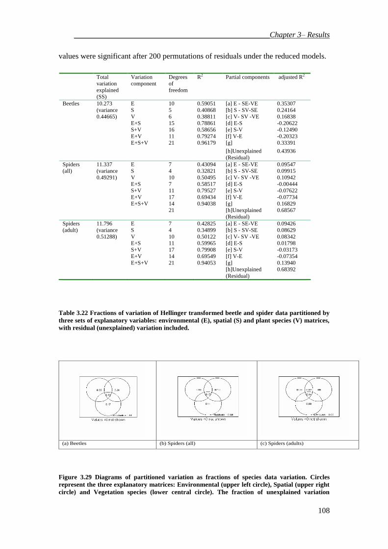
__________________________________________________Chapter 3– Results
108
values were significant after 200 permutations of residuals under the reduced models.
Total
variation
explained
(SS)
Variation
component
Degrees
of
freedom
R2 Partial components adjusted R2
Beetles 10.273 E 10 0.59051 [a] E - SE-VE 0.35307
(variance S 5 0.40868 [b] S - SV-SE 0.24164
0.44665) V 6 0.38811 [c] V- SV -VE 0.16838
E+S 15 0.78861 [d] E-S -0.20622
S+V 16 0.58656 [e] S-V -0.12490
E+V 11 0.79274 [f] V-E -0.20323
E+S+V 21 0.96179 [g] 0.33391
[h]Unexplained
(Residual)
0.43936
Spiders 11.337 E 7 0.43094 [a] E - SE-VE 0.09547
(all) (variance S 4 0.32821 [b] S - SV-SE 0.09915
0.49291) V 10 0.50495 [c] V- SV -VE 0.10942
E+S 7 0.58517 [d] E-S -0.00444
S+V 11 0.79527 [e] S-V -0.07622
E+V 17 0.69434 [f] V-E -0.07734
E+S+V 14 0.94038 [g] 0.16829
21 [h]Unexplained
(Residual)
0.68567
Spiders 11.796 E 7 0.42825 [a] E - SE-VE 0.09426
(adult) (variance S 4 0.34899 [b] S - SV-SE 0.08629
0.51288) V 10 0.50122 [c] V- SV -VE 0.08342
E+S 11 0.59965 [d] E-S 0.01798
S+V 17 0.79908 [e] S-V -0.03173
E+V 14 0.69549 [f] V-E -0.07354
E+S+V 21 0.94053 [g] 0.13940
[h]Unexplained
(Residual)
0.68392
Table 3.22 Fractions of variation of Hellinger transformed beetle and spider data partitioned by
three sets of explanatory variables: environmental (E), spatial (S) and plant species (V) matrices,
with residual (unexplained) variation included.
(a) Beetles (b) Spiders (all) (c) Spiders (adults)
Figure 3.29 Diagrams of partitioned variation as fractions of species data variation. Circles
represent the three explanatory matrices: Environmental (upper left circle), Spatial (upper right
circle) and Vegetation species (lower central circle). The fraction of unexplained variation

__________________________________________________Chapter 3– Results
109
appears as residuals.
The largest amount of explainable beetle variation (Table 3.22 and Figure 3.29a) was
explained by environmental variables (35%), while spatial variation explained 24%
and plant species explained the least (17%) beetle variation. Less of the variation of
spiders was explained by the three matrices which more or less equally explained
about 10% for all spiders and less than 10% for adult spiders. Residuals were high in
each case which indicated that unmeasured variables apart from spatial, plant species
and measured environmental variables had not been examined.
4.8.1 Identifying Species that account for variation
4.8.8.1 NMDS plus species biplots
(a) Beetles 3D stress 0.113

__________________________________________________Chapter 3– Results
110
(b) Spiders (all) 3D stress 0.124
(c) Spider (adult) 3D stress 0.167
Figure 3.30 NMDS plots of sites grouped in species space with biplots of species contributing
most to the clustering of sites indicated by the direction of the lines. Key to forest types: 1 =
WRE, 2= WOB, 3= DOB, 4 = DAM, 5 = DPU, 6 = DTO.
The stress levels of the ordinations in Figure 3.30 were high so only tentative
comments can be made about species whose variation in distribution contribute more

__________________________________________________Chapter 3– Results
111
highly to ordination of sites in species space.
The wetter WRE and WOB sites were separated along the horizontal axis by beetle
species that are mainly saprophages (Anotylus sp. B: Oxytellinae: Staphylinidae) and
fungivores (Acrotrichis sp.: Ptilidae and Thalycrodes australis (Germar, 1848):
Nitidulae along with a tiny (2mm) predator of these species (Homalotus sp B:
Aleocharinae: Staphylinidae) (Figure 3.30a). At the other end of the axis were
xylophagous weevils (Pachyporopterus satyrus (Pascoe, 1872): Curculionidae and
Mandalotus NM1: Curculionidae) which separated some of the drier DTO and DAM
sites. The tiny predatory Pselaphid species, Rybaxis NM7: Pselaphidae, separated
some sites along the vertical ordination axis. No clear patterns related to forest type
were discernable.
A separation of wet sites along the horizontal axis was discernable for all spiders
(Figure 3.30 b) and adult spiders (Figure 3.30 c) with the web builders Diplocephalus
cristatus (Blackwall, 1833): Linyphiidae and Amaurobiidae NM6: Amaurobiidae
separating some of the wetter sites. Drier sites were separated by vagrant hunters
(Storena flavipedes (Urquhart, 1893): Zodariidae, Gnaphosidae NM23: Gnaphosidae
and Suppuna NM1: Corrinidae). Vertically the sites were most strongly separated for
all spiders by the medium sized (15 mm) web builder Aaurobiidae NM2:
Amaurobiidae at one end of the axis, and the medium sized vagrant hunter
Gnaphosidae NM34: Gnaphosidae. A vertical separation of sites by adult spiders was
due to a mygalomorph spider (Migidae sp: Migidae) and web builder, Diplocephalus
sp. 1: Theridiidae, at one end of the axis and vagrant hunters at the other
(Gnaphosidae NM1: Gnaphosidae and Gnaphosidae NM13: Gnaphosidae).
4.8.8.2 Indicator species analysis
Indicator species analysis (Dufrene and Legendre, 1977) of abundance and occurrence
of a species in one group compared with all groups (McCune and Grace) was

__________________________________________________Chapter 3– Results
112
performed in R with a Monte Carlo random reshuffling test of significance for 1000
permutations.
Species code FOREST TYPE Observed IV IV From randomised groups
Avg Max WRE WOB DOB DTO DPU DAM Mean S. Dev p
Nargo 8 50 50 0 0 0 0 0 50 24.5 9.68 0.126
ZeadoNM2 13 75 75 0 0 0 0 0 75 22.1 11.96 0.014
Galerby 4 25 25 0 0 0 0 0 25 25 0.79 1
Agrypnus 8 38 0 0 0 13 38 0 37.5 24.6 13.02 0.355
Noto 8 50 50 0 0 0 0 0 50 23 10.74 0.137
Seringra 4 25 0 0 0 0 25 0 25 25 0.79 1
Maydena 4 25 0 25 0 0 0 0 25 25 0.79 1
CrypNM8 4 25 0 0 0 25 0 0 25 25 0.79 1
Aleohomf 8 50 0 0 0 50 0 0 50 22.4 10.11 0.119
Table 3.23 Potential indicator beetle species for different forest types.
The beetle dataset was reduced from 152 to 49 species to remove rare species whose
abundances were too low (less than 5 across all sites) to enable significant indications
about associations with particular forest types. Nine beetle species (Table 3.23) were
potential indicators of a particular forest type but only Zeadolopus NM2 , was
statistically significant (p = 0.0140). It was an indicator of WRE.
All Spider
species FOREST TYPE
Observed
IV IV From randomised groups
Avg Max WRE WOB
DOB DTO DPU DAM Mean S. Dev p
AMAUNM1 8 44 0 0 3 44 0 4 43.7 20.9 12.61 0.141
GNAPNM3 4 25 0 0 25 0 0 6 25 25 0.79 1
GNAPNM4 4 25 0 0 25 0 0 6 25 25 0.79 1
GNAPNM14 8 50 0 0 0 0 50 5 50 23.8 9.99 0.127
GNAPNM17 8 50 0 0 0 50 0 4 50 17.7 13.03 0.141
GNAPNM36 4 25 0 0 25 0 0 6 25 25 0.79 1

__________________________________________________Chapter 3– Results
113
Table 3.24 Potential indicator spider species.
The all spider dataset was reduced from 204 species to 54 to exclude those
represented by only 5 individuals or less across all sites. Based on their presence in
only one forest type, (Table 3.24) only six species were contenders for indicators of
forest type, but none were statistically significant.
4.8.1 Regional variation
The question addressed in this section is whether the variations in species
assemblages that were noted in one geographical area can be generalized across much
greater distances within the same region. Variation in species assemblages at groups
of sites in three widely separated regions 50 km apart (Hobart, Levendale and
Swansea) were compared.
Nonparametric Manova tests were conducted with PERMANOVA (Anderson, 2005)
for a two-way fixed-factor ANOVA with factors ‘Region’ and ‘Forest type’ and a
balanced design. There were six replicates. The analysis was based on Bray-Curtis
dissimilarities of data transformed to ln (x+1). Results were tested with 9999
unrestricted permutations of the raw data.
Non-parametric Multivariate Analysis of Variance
Variables Source df SS MS F P
Beetles Region 2 9188.5927 4594.2964 2.4503 0.0002
186 spp Forest
RegionxForest
Residual
1
2
30
2475.4637
11345.4397
56250.8545
2475.4637
5672.7198
1875.0285
1.3202
3.0254
0.1936
0.0001
Total 35 79260.3506
Spiders Region
Forest 2
1 9129.6481
1455.2956 4564.8241 1455.2956
1.8352 0.5851
0.0110
0.9030
(all) RegionxForest
Residual 2
30 9524.2403
74620.9716 4762.1201 2487.3657
1.9145 0.0070
196 spp Total 35 94730.1555
Spiders Region
Forest 2
1 10418.2080
2627.6830 5209.1040 2627.6830
1.8908 0.9538
0.0150
0.4900
(adults) RegionxForest
Residual 2
30 11720.7876
82651.1659 5860.3938 2755.0389
2.1272 0.0060
182 spp Total 35 107417.8445
Table 3.25 Results of permutational non-parametric multivariate analysis of variance for sampled regional groups. Residuals were used in the denominator of MS for the F-ratio.

__________________________________________________Chapter 3– Results
114
There was a significant difference between species assemblages in different regions
(p= 0.0002 for beetles, p= 0.0110 for all spiders and p= 0.0150 for adult spiders)
(Table 3.25), which pairwise a posteriori comparisons (Table 3.26) revealed were
consistently due to significant differences between the regions that were furtherest
apart, Hobart and Swansea. The intermediate region, Levendale did not host
significantly different assemblages.
Taxa Factors t P (permut) P MC Sig. Level
Beetles Region (Hbt, Lev) 1.6841 0.007 0.019 0.117
Region (Hbt, Swa) 1.7589 0.009 0.16 0.025 Region (Lev, Swa) 1.2271 0.055 0.161 0.05 Forest by Region: Hbt (DOB, DPU) 1.3097 0.069 0.087 0.05 Forest by Region: Lev(DOB, DPU) 1.5894 0.002 0.012 0.05 Forest by Region: Swa(DOB, DPU) 1.5048 0.012 0.027 0.05
Spiders Forest by Region: (Hbt, Lev) 0.9055 0.663 0.546 0.05 Region (Hbt, Swa) 1.5453 0.033 0.034 0.117 (all) Region (Lev, Swa) 1.0891 0.267 0.319 0.025 Forest by Region: Hbt(DOB, DPU) 1.3263 0.06 0.77 0.05 Forest by Region: Lev(DOB, DPU) 1.6477 0.003 0.008 0.05 Forest by Region: Swa(DOB, DPU) 0.9546 0.567 0.519 0.05
Spiders Region (Hbt, Lev) 1.4443 0.039 0.045 0.025 (adults) Region (Hbt, Swa) 1.6595 0.005 0.007 0.117 Region (Lev, Swa) 0.809 0.8219 0.736 0.05 Forest by Region: Hbt(DOB, DPU) 0.9508 0.513 0.455 0.05 Forest by Region: Lev(DOB, DPU) 1.7556 0.007 0.012 0.05 Forest by Region: Swa(DOB, DPU) 1.1321 0.222 0.266 0.05
Table 3.26 Results of pair-wise a posteriori comparisons for permutational non-parametric
multivariate analysis of variance. The significance levels have been Bonferoni corrected for
multiple comparisons.
The differences in assemblages in different forest types was not significant for the
whole region (p = 0.1936) but when forest types were broken down into regions by a
posteriori tests (Table 3.26), beetle assemblages were significantly different between
forest types in Levendale (0.0090) and Swansea (0.0070). This is supported by a
significant multivariate interaction between the factors ‘Region’ and ‘Forest’ (p=
0.0001) reported in Table 3.25. Beetles and spider assemblages were significantly
different in among forest types DOB and DPU in the Levendale region. None of the
multivariate assemblages showed a difference in DOB compared with DPU forest
types in the Hobart region and only beetles were significanly different among forest
type in the Swansea region.
Nonmetric Multidimensional Scaling methods (NMDS) provided a visual clue to how
closely sites from the same region clustered in species space across large distances.

__________________________________________________Chapter 3– Results
115
Stress for all plots was very high so they should not be interpreted in detail, but they
do portray the failure of sites in the same region to cluster together which
demonstrates those sites do not share a greater number of similar species.
(a) Beetles 1D stress 55.22763 (b) Spider (adult) 3D stress= 19.39610
Figure 3.31 NMDS ordination of regional sites in species space with regional groups indicated:
▲Hobart, ♦ Levendale and ■ Swansea.
Ordinations of the data demonstrate an overall random stucture of species
assemblages which do not correspond to region (Figure 3.31) or forest type (Figure
3.32), though adult spiders do indicate some separation of sites by forest type (Figure
3.32 c).
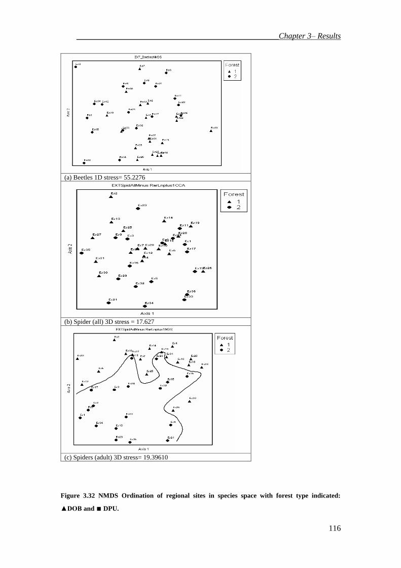
__________________________________________________Chapter 3– Results
116
(a) Beetles 1D stress= 55.2276
(b) Spider (all) 3D stress = 17.627
(c) Spiders (adult) 3D stress= 19.39610
Figure 3.32 NMDS Ordination of regional sites in species space with forest type indicated:
▲DOB and ■ DPU.

__________________________________________________Chapter 3– Results
117
4.8.9.1 Regional autocorrelation
The Mantel test results compare dissimilarity in geographic distance between pairs of
sites with Bray-Curtis species dissimilarity (Figure 3.33). The value of rho for all
assemblages was low, i.e. less than 0.18 (p= 10005), which indicates that sites that
were proximate did not necessarily contain a greater number of similar species. This
trend was also evident at the scale of the Mt Wellington sites that spanned less than 2
km. The regional sites spanned 157 km with approximately 50km separation between
each of the regional groups of sites.
(a) Beetles Rho = 0.178356, p = 0.005 (b) Spiders (all) Rho = 0.148463, p = 0.005
(c) Spiders (adults) Rho = 0.167962, p = 0.005
Figure 3.33 Mantel test: Plots of distances between pairs of regional sites against species
dissimilarity between pairs of sites (Bray-Curtis) for each of the multivariate species matrices:
beetles, spiders (all) and spiders (adults). Spearman’s Rank correlation coefficient (rho) appears
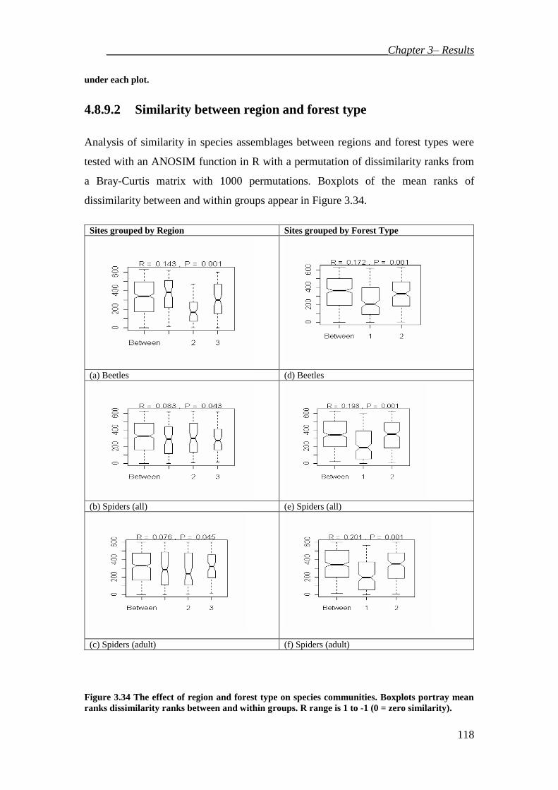
__________________________________________________Chapter 3– Results
118
under each plot.
4.8.9.2 Similarity between region and forest type
Analysis of similarity in species assemblages between regions and forest types were
tested with an ANOSIM function in R with a permutation of dissimilarity ranks from
a Bray-Curtis matrix with 1000 permutations. Boxplots of the mean ranks of
dissimilarity between and within groups appear in Figure 3.34.
Sites grouped by Region Sites grouped by Forest Type
(a) Beetles (d) Beetles
(b) Spiders (all) (e) Spiders (all)
(c) Spiders (adult) (f) Spiders (adult)
Figure 3.34 The effect of region and forest type on species communities. Boxplots portray mean
ranks dissimilarity ranks between and within groups. R range is 1 to -1 (0 = zero similarity).

__________________________________________________Chapter 3– Results
119
Key – Region: 1 = Hobart, 2 = Levendale, 3 = Swansea; Forest: 1 = DOB, 2 = DPU.
Boxplots of data classified by forest type (Figure 3.34) portray the wide variation in
data as exemplified by the width of the plots. The R values were all significant for
each plot. The R values for spider dissimilarity when grouped by Region (left hand
side plots) were both close to zero which indicates that there is a strong difference in
spider species within regions. The difference was slightly less strong for beetles (R=
0.143). The differences when grouped by forest type were again fairly strong for
spiders and beetles with R values around 0.2.

__________________________________________________Chapter 3– Results
120

__________________________________________________Chapter 3– Results
121

__________________________________________________Chapter 4 – Discussion
122
Chapter 4 Discussion
Several themes emerged from statistical analysis of data collected for this study.
These themes, discussed below, lead to an understanding of the underlying finer scale
of interactions between environment, space and species that are summarised as
‘biodiversity’, an assessment of which forms the basis for planning decisions.
Many of the statistical tests conducted produced significant results indicating some
degree of association between forest type and species. This significance, however,
does not imply that distributions of spiders or beetles simply correspond to forest type
and illustrates the wrong conclusions that may be drawn from data that are not well
interrogated.
Statistical output indicated that some species within assemblages were responsible for
these associations while others were not. Thus an assemblage cannot be viewed as a
collection of species that interact in the same way and respond in the same way to
their environment. This was supported by seasonal variation in species (Figures 3.12
and 3.13 for beetles, and Figure 3.17 for spiders) and investigation of trophic level
variation in beetles (Figure 3.14) and hunting styles in spiders (Figure 3.19).
Several tests (NP-MANOVA, CAP and ANOSIM) aimed to find significance in the
distribution of multivariate species data grouped by forest type. Each test revealed that
association with forest type did not always apply to all species within an assemblage
or to all forest types in the study. Each test also revealed different detail about the
distribution of each taxa which enabled further exploration as outlined.
NP-MANOVA detected a significant difference between assemblages of beetles and
spiders in different mapped forest types (p= 0.0002 for each analysis). Pairwise a
posteriori tests revealed that significant differences were not consistent across all
forest types. Complete correspondence of particular assemblages with particular forest

__________________________________________________Chapter 4 – Discussion
123
types was lacking.
Beetle assemblages in DTO and DAM were significantly dissimilar to those in wet
WRE (p= 0.0291 and p= 0.0316 respectively), WOB (p= 0.0298 and p= 0.0276
respectively) and DOB (p= 0.0262 and p= 0.316 respectively). Assemblages of
beetles in DPU were not significantly different to those in any other forest type. An
illustration of these relationships appears in Figure 4.1.
In addition WRE also hosted assemblages significantly different to those in DOB (p=
0.0308).
Figure 4.1 Representation of forest types from a posteriori NP-MANOVA comparisons of
dissimilarity between beetle assemblages in mapped forest types. No overlap of circles represents
distinct beetle assemblages
Beetles identified as responsible for multivariate variation from the canonical axes of
the CAP analyses were Nemadini: Leiodidae, Scaphidium sp.:Staphylinidae,
Thalycrodes australe (Germar, 1848): Nitidulae, Acrotrichis sp. (Ptilidae), Isopteron
abscurum (Erichson, 1842): Tenebrionidae and Tetrabothrus claviger (Fauvel, 1878):
Staphylinidae.
For all spiders seven species were correlated to some degree with the canonical axes,
suggesting they may be responsible for some of the multivariate distribution patterns.
They were Suppuna picta (Koch, 1873), Gnaphosidae NM34, Gnaphosidae NM37,
Micropholcommatidae NM8, Lycosidae NM1, Zodariidae NM26 and Zoridae NM1.
It should be observed that these species are all vagrant hunters except
DTO
P
WRE
WOB
DOB DPU
DAM

__________________________________________________Chapter 4 – Discussion
124
Micropholcommatidae sp. which is a tiny (1.5 mm) web building spider. The
distribution of these spiders would be expected to vary according to prey availability
and habitat. They all require ground cover such as litter, rocks, coarse woody debris,
logs or moss.
There was a general dissimilarity in spider (adults) assemblages from wetter forest
types compared to those in drier forest types. However, there was additional
separation between the wet sites themselves with WOB dissimilar to all other forest
types. This suggests that important factors are more complex than a simple moisture
gradient. Wet WRE was significantly dissimilar to all other forest types except dry
DOB which was nearly significantly different (p = 0.0564). These relationships are
illustrated in Figure 4.2. The distribution of only one adult spider species,
Hestimodema A (Zoridae) correlated with any significance with the canonical axes.
Hestimodema A is another vagrant hunter that lives under litter, rocks, coarse woody
debris or logs.
Figure 4.2 Representation of forest types from a posteriori NP-MANOVA comparisons of
dissimilarity between spider assemblages in mapped forest types. No overlap of circles represents
distinct spider (adults) assemblages.
Examining the dispersion of the data was valuable in determining the extent to which
the significant effects of forest type found in NP-MANOVA were due to differences
in location or differences in spread of the data (Anderson, 2004).
DTO
P
WRE
WOB
DOB
DPU
DAM

__________________________________________________Chapter 4 – Discussion
125
Multivariate dispersion of the adult spider data was not significantly different among
groups of forest type (p= 0.5271), so forest type itself had an effect on assemblages to
the extent revealed by the a posteriori NP-MANOVA comparisons discussed above.
Mutivariate dispersion of the beetle data was significant (p= 0.0244) which means
that there was a significant amount of dispersion in the beetle data between groups so
forest type per se did not necessarily account for the significant NP-MANOVA
results. Once again, significant effects cannot be assumed to be the same across all
forest types studied as shown by DTO forest type which seemed to be largely
responsible for the dispersion. One conclusion of this analysis is that high dispersion
due to high variation in assemblages within a particular forest type implies that factors
other than forest type are influencing species distributions.
Canonical analysis of Principal co-ordinates (CAP) with discriminant analysis (DA)
indicated that forest type was not significant for beetles, (the very low squared
canonical correlation (δ2) of 0.069088 which was not significant (p= 0.8558)).
Forest type was highly significant for all spiders, with δ2 = 0.909598 (p= 0.0011) but
was no longer significant when only adult spiders were considered (squared canonical
correlation (δ2
= 0.385911, p= 0.3944).
The leave-one-out cross validation test had generally poor success in correctly
allocating species to forest type, suggesting high variability in assemblages in most
forest types, see Table 3.18. Successful beetle allocation was highest (75%) for WOB
and DAM and lowest for DOB and DPU (25% and 0% respectively).
All spiders in forest type WRE were correctly allocated (100%) with high allocations
(75%) for WOB and DOB. Zero successful allocation of all spiders to DPU and DAM
reinforce the finding that spider assemblages are highly variable in these forest types.
When only adult spiders were considered, they were successfully allocated (75%) to

__________________________________________________Chapter 4 – Discussion
126
WRE WOB and DAM but were unable to be successfully allocated (0%) to DOB.
Again differences in distributions of species are revealed when juveniles are included
with adult spiders.
Canonical correlation of species distribution and environmental variables provided
some interesting insight into the adequacy of the environmental variables measured
because they were thought a priori to be important. The resulting subset of beetles
most highly correlated with forest type alone was dominated by fungivores:
Nemadini, Thalycrodes australe (Germar, 1848), Acrotrichis sp. and Scaphidium sp.
(Table 4.1).
Correlated with
Forest type
Correlated with Environmental
variables
beetles Nemadini Nemadini
Thalycrodes australe Thalycrodes australe
Acrotrichis sp. Thalycrodes cylindricum
Scaphidium sp.. Scaphidium sp.
Isopteron obscurum Zead NM2
Tetrabothrus claviger Rybaxis rugosus
Mandalotus NM1
Anotylus B
Spiders Suppuna picta Suppuna NM1
(all) Gnaphosidae NM34 Gnaphosidae NM1
Lycosidae NM1 Laetesia NM1
Micropholcommatidae NM8 Mynogleninae NM33
Zodariidae NM26 Storena flavipes
Zoridae NM1 Zodariidae NM12
Table 4.1 Species whose distribution was found, by canonical analysis of principal coordinates, to
be correlated with forest type (column 2) or with the set of environmental variables (column 3).
The appearance of some beetles in both lists suggests that they might respond to
environmental variables that are correlated with forest type, for example canopy
cover; or they might respond to other environmental variables in addition to forest
type. Earlier, Isopteron obscurum (Erichson, 1842) and Tetrabothrus claviger
(Fauvel, 1878) were identified among those whose distribution corresponded to forest
type to some degree. The current analysis separates them from the others in that list
(Table 4.1) which were all fungivores. This means that none of the environmental
variables measured in this study significantly explained their distribution beyond

__________________________________________________Chapter 4 – Discussion
127
forest type. Since the correlation of canonical axes with the species distribution was
0.6621 and 0.6381 respectively, there are still unknown variables contributing to their
distribution beyond those in this research.
It is possible to represent these associations of beetles as follows (Figure 4.3):
Figure 4.3 Representation of beetles whose distributions, from canonical correlation, are
correlated with mapped forest type or measured environmental variables or both.
Some beetle species that were correlated with environmental variables were not
highly correlated with any of the canonical axes discriminating among forest type,
namely Rybaxis rugosus, Thalycrodes cylindricum Blackburn, 1891, Mandalotus
NM1 and Anotylus B.
PCA analysis of environmental variables produced a reduced set of variables that
corresponded to most to differences between sites. BIOENV identified a similar set of
variables that correlated strongest with the biotic data (Table 3.21). NMDS
ordinations (Figure 3.25) provided a basis for distinguishing among the effects of the
variables by indicating environmental gradients which are summarised in Figure 4.4.
FOREST TYPE
Isopteron obscurum
Tetrabothrus claviger
Rybaxis rugosus
Thalycrodes cylindricum
Mandalotus NM1
Anotylus B
ENVIRONMENTAL
VARIABLES
Nemadini
Thalycrodes australe
Scaphidium sp.

__________________________________________________Chapter 4 – Discussion
128
BEETLES
SPIDERS
Figure 4.4 Diagrammatic representation of environmental gradients identified as associated with
beetle and spider assemblages.
Beetles seemed to correspond to a moisture gradient which, at the wetter end, most
strongly correlated with canopy cover and created a microclimate suitable for
increased fungi volume, ferns and broad leaf shrubs. Canopy cover and soil moisture
have been identified by other researchers as variables that affect the distribution of
beetles (Magura 2002; Niemela and Spence 1994; Oliver et al. 2000). The finding that
beetle species richness was lower in the more open canopy of the drier forests and
higher under the more closed canopy of wetter forests (Figure 3.20) supports results
High canopy cover
Ferns
Higher fungi volume
Broad leaf shrubs
Higher solar radiation
Higher litter temperature MOISTURE GRADIENT
High coarse woody debris
Deeper organic soil layer
Higher phosphorous in
top soil
Shrub cover at ground
level
Soil hardness,
Area of bare ground
Rocky subsoil
Higher humidity at ground level
Higher soil moisture
Broad leaf shrubs
Higher solar radiation in winter
Higher subsoil temperatures in
winter
Higher litter temperature in winter
Higher levels of nitrogen
in top soil
Higher minimum nitrogen
levels in the subsoil
Higher C:N ratio in
top soil
GROUND COVER GRADIENT
TEMPERATURE GRADIENT
SOIL NUTRIENTS GRADIENT
SPIDERS

__________________________________________________Chapter 4 – Discussion
129
of Oliver et al. 2000. Oliver et al. (2000) also found that ants, like the spiders in this
research, had an inverse relationship to canopy cover compared with beetles, and
displayed lower species diversity in wet forests and increased diversity under low
canopy cover. Environmental variables such as ground temperature, surface
temperature, air moisture, cover of leaf litter, herbs, shrub and canopy layer have been
identified as significant for carabids (Magura 2002).
Variables not measured which are likely to be associated with this environment
gradient include mosses and lichens which host a number of beetles from families
found in this study such as Byrrhidae species (Lea 1920), weevils e.g. Mandalotus
bryophagus, Mandalotus carinativentris (Lea 1907) and Scydmaenidae e.g.
Scydmaenus seminiger, Phagonophana suturalis (Lea 1914) and Pselaphids e.g.
Euplectops bryophilis Lea, 1911, Sagola tasmaniae Lea, 1911 and Schistodactylus
brevipennis Lea 1911 (Lea 1911). A moist microclimate would increase presence of
litter herbivores which may be prey for predatory beetles. The microclimate would
also increase litter fungi which would sustain fungivorous beetles such as Thalycrodes
spp., Leiodidae and Lathridiidae. The drier end of the gradient was associated with
higher solar radiation on the ground (due to lower canopy cover), and higher litter
temperature. A ground cover gradient was identifiable for beetles where increased
ground cover was associated with high levels of coarse woody debris, increased depth
of top soil and higher levels of phosphorus in the top soil. These findings support
those of Oliver et al. (2000) who identified similar variables such as percent cover of
subcanopy and the cover of the ground layer (litter depth, bare soil and rock) that
explained significant variation in ground beetles and spiders. Several beetle families
have an obligate association with CWD (Dajoz 2000; Grove 2002, Yee et al. 2001),
including Buprestidae, Cerambycidae, Bostrichidae, Brentidae and the Curculionids
Scolytinae and Platypodinae (Ulyshen et al. 2004), while Leiodidae feed on fungi and
slime moulds associated with CWD (Chandler and Peck 1992).
Spiders were correlated with a moisture gradient that separated spiders associated
with higher humidity at ground level, higher soil moisture and broad leaf shrubs at
one end from higher radiation at ground level (due to less canopy cover), higher

__________________________________________________Chapter 4 – Discussion
130
subsoil temperatures in winter and higher litter temperature in winter. The higher
temperatures variables would favour active spiders such as vagrant hunters. A second
gradient, soil nutrients, associated spiders in wetter sites with higher levels of nitrogen
in the top layer of soil (A horizon) and higher minimum levels of nitrogen in the
subsoil (B horizon). Spiders in the drier sites were associated on the soil nutrient
gradient with a higher carbon to nitrogen ratio in the top soil layer (A horizon).
It may seem curious that distributions of spiders and beetles might correspond to soil
nutrients, however available phosphorus levels are known to increase following nest
material accumulation by ants (Frouz et al. 2005; Kristiansen et al. 2001), and
passage of organic material through the gut of soil macrofauna such as scarab beetle
larvae (Li et al. 2006) and earthworms (Sharpley and Syers 1977). Beetles associated
with raised levels of phosphorus are likely to be predators of soil macrofauna such as
ants and beetle larvae that are active in raising these nutrient levels. The more
numerous predatory litter beetles in this study include Notonomus politulus
(Chaudoir, 1865): Carabidae.
Soil nitrogen levels are increased by several factors including ant activity in nests
(Lenoir et al. 2001), litter herbivore activity (Chapman 2003; Hunter et al. 2003) litter
bacteria and litter and wood-rotting fungi (Lindahl et al. 2007). Increased nitrogen
lowers the C:N ratio. Spiders associated with raised levels of N may be predators of
ants, litter herbivores and fungivores and in this study would include vagrant hunters
in the families Corrinidae, Lycosidae and Clubionidae, as well Linyphiidae which, as
web spinners, build small webs on structural elements at ground level, including rocks
and stones (Nentwig 1980) and are particular predadators of collembola. Several dry
sclerophyll plant species in this research such as eight Acacia spp., Daviesia ulicifolia
and five Pultenaea spp. are amongst those known to contain root nodules that host
symbiotic microrganisms that fix nitrogen and increase its availability to the
environment (Bowen 1986). There may be associations between some vagrant spiders
and sources of prey that inhabit these species of plants.

__________________________________________________Chapter 4 – Discussion
131
The variation in environmental variables between beetles and spiders indicate
different uses of their habitat. For example the volume of rotting wood was amongst
the most highly correlated variables for spiders and beetles (Table 3.21). At the
ecological level this suggests a correlation with beetle species that breed in and feed
on rotten wood (saprophages). Spider species inhabiting rotten wood may be
specialised predators of occupants of rotten wood.
The absence of certain species of beetles in the relatively undisturbed habitat
fragments sampled in this study were consistent with findings from other studies
(Baker 2006; Grove and Yaxley 2005; Michaels and McQuillan 1995; Michaels
1999). Beetles associated with regenerating forests, were present only as a singelton
(Mecyclothorax ambiguus (Erichson, 1842) or absent (Scopodes sigillatus Germar,
1848 and Rybaxis parvidens Lea, 1911) (Baker 2006; Michaels and McQuillan 1995;
Michaels 1999). Notonomus politulus (Chaudoir, 1865), a specialist of old-growth
forest (Michaels and McQuillan 1995) was found in this study.
Little is known of the ecology and distribution of many beetles and, more particularly,
spiders. For example, two spider species of the Nicodaemidae family that are known
to be widely spread in Tasmanian forests, were found in this study - Ambicodamus
sororius (Harvey, 1995) and Novodamus nodatus (Karsch, 1878). N. nodatus is
described as an inhabitant of closed wet forest where its habitat includes underneath
stones, under bark of eucalypts and dead wattles, shrubs and litter (Harvey, 1995). In
this study both species were found at sites in dry eucalypt forest types with less than
50% canopy cover and a third, unnamed, species of Nicodaemidae was also found. In
the extensive study Nicodaemidae were only found in E. pulchella forest in the
Levendale region with A. sororius totally absent from the regional samples. With so
little known about species it is difficult to predict their distribution. This research
aimed to reveal some variables that enable distributions of invertebrates to be
predicted as an aid to the planning of reserves.

__________________________________________________Chapter 4 – Discussion
132
Species richness differences in similar habitats are frequently indicators of
disturbance (Broque and Buckney 2003; Gibb and Hochuli 2002; Harris et al. 2003)
or pollution (Clarke and Ainsworth 1993; Deeleman-Reinhold 1990) but are not a
viable basis for selection of terrestrial reserves across a landscape where differences
in composition of assemblages must be considered (Su et al. 2004). Spiders in this
research, for example, were more diverse in dry forest types, but their species
diversity was lower yet significantly different in wet forest types. Species would be
lost if wet forests weren’t also reserved.
Planners have focused on the objective of reserving a representative diversity of
species which has been tackled in a variety of ways. A minimum representation goal
has derived site scores from multiple criteria such as species diversity and rarity,
condition and area of habitat etc to provide a priority index to identify the minimum
number of sites required to maximize reserved biodiversity (Possinghham et al. 2000;
Pressey and Nicholls 1989). A similar complimentarity approach (Faith and Walker
1996; Faith et al. 2003; Justus and Sarkar 2002; Oliver et al. 1998) iteratively
reweights attributes of species occurrences or habitats as sites become prioritised for
reservation so that additional sites contain attributes not already reserved (Bedwood et
al. 1992; Kirkpatrick 1983; Possingham et al. 2000) based on the composition of
assemblages and inclusion of rare species (Margules 1989). Algorithms used to create
site scores have been based on subjectively differently measured parameters, pattern
analysis (McKenzie et al. 1989) and statistically derived regression models based on
correlated variables (Lindenmayer and Cunningham 1996; Margules and Stein 1989).
Different methods have created variable results when ranking sites for reserves
(Kirkpatrick 1983; Margules and Stein 1989: Possingham et al. 2000; Pressey and
Nicholls 1989) and selection of the minimum reserve set is not necessarily sufficiently
robust under temporal species turnover where local extinctions may occur (Rodriges
et al. 2000).
The minimum representation focus on planning has been largely descriptive of the
biotic and abiotic features at the time they were measured or assessed. At the same

__________________________________________________Chapter 4 – Discussion
133
time collection of data on changes in species distributions is costly and time
consuming. One tool which has become useful to planners considering reserves in a
fragmented landscape is the minimum fragmentation threshold which is a measure of
habitat area below which a species may be lost (Drinnan 2005). Its value has been
questioned (Hugget 2005; Lindenmayer et al. 2005; Lindenmayer and Luck 2005) as
perhaps encouraging no more than a minimum area to be reserved while the minimum
habitat size will depend upon the condition if the remnant (McCoy and Mushinsky
2007). Environmental domain analyses (Belbin 1993; Mackey et al. 1988) based on
‘ecologically relevant environmental variables’ as surrogates for species distribution
data (Kirkpatrick and Brown 1994) have been successfully applied to vegetation data
and are a basis for GIS modelling of potential habitat of specific species and spatial
prediction using geostatistics (Cabeza et al. 2004; Dettmers and Bart 1999; Hengle
2007).
Modelling has been attempted across scales from point collected species data which
are affected by fine scale environmental changes to the macro-scale of landscapes and
their connectivity (Urban 2005). An increasing focus on landscape ecology faces
planners with challenges as they consider biodiversity across the broader landscape
which is not static and where land clearing, fire, habitat fragmentation and so on are
altering biotic and abiotic dynamics. Landscape metrics that characterise landscape
patterns are being refined to provide information for modelling landscape processes
(Debuse et al. 2007; DiBarri 2007; Hargis et al. 2004; McAlpine and Eyre 2002)
including scaling equations (Wu et al. 2002). It was difficult for the current research
on spiders and beetles to identify patch-scale variables that accounted for most of the
variation in assemblages. This emphasises the difficulty in achieving adequate
landscape-scale metrics. The challenge is to identify non-redundant variables whose
gradients are highly variable and therefore useful for distinguishing between different
landscapes. Predictive models that enable scenario planning frequently make use of
Bayesian paradigms (Calder et al. 2003; Clark 2005; Hobbs and Hilborn 2006) using
probability distributions of measured parameters (Borsuk et al. 2001; Kerman and
Gelman 2007; Latimer et al. 2006; Martin et al. 2005) and qualitative predictions

__________________________________________________Chapter 4 – Discussion
134
(Dambacher et al. 2003).
It should also be recognised that the scale of impact from threatening processes such
as land clearing and habitat fragmentation is much larger for invertebrates (Hutchings
and Ponder 1999) and we must not lose sight of the purpose for reserving biodiversity,
which is to build the resilience of ecosystems to survive threatening processes.
4.8.1 Regional variation
The measure of species diversity at different geographic scales was found to vary
considerably, which supports the view that different species respond to habitat at
different spatial scales (Holland et al. 2004; Yaacobi and Ziv 2007). Assemblages
were sampled in three regions approximately 50 km apart and provided a comparison
of diversity at the local scale of 1km in the Mt Wellington study with differences in
species present regionally at the scale of fifty kilometres, and for the entire region
sampled, at the scale of 150 kilometres. Using a modified Whittaker’s beta diversity
index, it was observed that beta diversity was higher for beetles and spiders (25 and
29 respectively) than for plants (7) and fungi (15) at the local scale of a kilometre
(Table 4.2). The beta diversity of beetles and spiders was highest at the scale of 50
km (range from 30 to 42), and lowest at the scale of 150 km (range 16 to 19) (Table
4.2 ).
diversity index
Taxa Local scale (1km) Regional scale (50km) Extensive scale (150 km)
beetles 24 36 - 40 19
spiders (all) 29 29 - 38 16
Spiders (adults) 29 30 - 42 17
Fungi 15 n/a n/a
Plant spp. 7 n/a n/a
Table 4.2 Variation in beta diversity measured at different scales. n/a means data was not
available at the regional scale.
The low beta diversity in plants was not reflected by invertebrates for which there
were large differences in assemblages. This provides evidence that plants and

__________________________________________________Chapter 4 – Discussion
135
invertebrates need to be considered differently when planning for conservation of
biodiversity (Mesibov 1993; Oliver et al. 1998). Geographic distances at which
measures of diversity are applied must also be recognised.
Spiders and beetles demonstrate some differences in their distributions and may be the
case that when this data is analysed against concurrently collected ant data (Meeson
2006) that further different distributions of invertebrate assemblages are identified.
Oliver and Beattie (1996), for example, recommend that ant and beetle data be
combined for an accurate characterisation of invertebrate assemblages. Oliver et al.
(2000) conclude that ant richness has more potential than beetle richness as a
performance indicator of sustainable forest management because ant assemblages can
be more accurately and quickly represented by pitfall sampling because of their higher
foraging activity compared with beetles.
Non-parametric multivariate analysis of variance indicated that there was a significant
difference in assemblages between the Hobart and Swansea regions (Table 3.25), with
overlap of species in the intermediate Levendale region. When regions were
considered together, at the scale of 150 km, assemblages were not significantly
different between the two forest types (DOB and DPU), but when considered by
region, assemblages in different forest types were significantly different between
Swansea and Levendale. The differences in assemblages in DOB and DPU forest
types were also not detectable at the local scale of 1km (Tables 3.13 and 3.15). This
indicated that the scale of 50 km was the resolution at which the more subtle
differences between assemblages in different dry forest types could be detected. The
possibility of creating connectivity within forest types studied in this research would
be challenging due to their patchy, limited distribution (Figure 2.3) and threats from
loss of dry eucalypt forests to fuelwood, logging, land clearing for agriculture and
coastal development (Brown and Podger 1999; Williams 1991). Keitt et al. (1997)
present a method for quantifying conservation priority of fragmented habitat patches
that contribute most to connectivity, based on dispersal abilities of species, connection
probabilities and percolation theory.

__________________________________________________Chapter 4 – Discussion
136
4.8.1 Including juvenile spiders in ecological studies.
It is possible to include juvenile spider data if a family level of resolution of a spider
sample is required (New 1999) since, for some research questions, family level
analysis is adequate (Churchill 1995). It is more usual to exclude juvenile spiders
from samples because of the difficulty in identifying them to species level
(Coddington et al. 1996; Harris et al. 2003; Oxbrough et al. 2005; Uetz 1977). A
third (34%) of all spiders sampled in this study were juveniles with statistical analyses
conducted on ‘all spiders’ sampled and ‘adults only’. The purpose was to explore the
possibility that the inclusion of juveniles may provide more power for statistical
analysis.
The inclusion of juveniles created 17 families in addition to the 183 families of adults.
Each family of exclusively juvenile spiders was represented by a maximum of three
individuals, and more usually one or two individuals. These families were routinely
excluded from analyses where rare species (represented by less than five individuals)
are not included because their abundance is insufficient to show any distribution
patterns. The inclusion of juveniles with identified adults would have been a source of
error by inflating abundance of certain species even though a fairly strong ln (x+1)
transformation of data was usually selected to reduce dominance of abundant species.
Results of analyses varied depending on whether juveniles were included or not. For
example, the inclusion of juvenile spiders reduced the correlation of spiders with
forest type from R = 0.417 to R = 0.396 and increased the variability of assemblages
between sites within the same forest type (see boxplots Figure 3.22). Adult spiders
showed a stronger significant association with a larger number of environmental
variables than when juveniles were included (Table 3.21). Variables not significant
when juveniles were included were shrub cover, soil hardness and volume of rotting
wood. This could be due to a number of factors related to dispersal mechanisms

__________________________________________________Chapter 4 – Discussion
137
among spiders whereby juveniles are found in a larger range of microhabits that they
may traverse before selecting a suitable niche. The fact that they were sampled at a
particular site does not imply an association. Alternatively, use of habitat or activity
level may vary during the lifecycle of some species. Seasonal variation in abundance
of juvenile spiders (Figure 3.17) shows a decrease in the summer which, apart from
natural losses through competition and predation, may be due to maturation. Certainly
when making cross-taxon comparisons of pitfall sampled beetles, ants and so on it is
usually adults that are compared (Gibb and Hochuli 2002; Major et al. 1999; Oliver et
al. 1998).
Therefore, rather than excluding juvenile spiders from research results because they
present taxonomic problems, this research provides statistical analysis that points to
ecological reasons for their exclusion.
Textricella hickmani Forster, 1959 Phoroncidia sp. Micropholcomma sp.
Micropholcommatidae Theridiidae Micropholcommatidae
(adult male) (juvenile male) (adult male)

__________________________________Chapter 5 – Implications and Conclusions
138
Chapter 5 Implications and Conclusion
This study contributes to knowledge about the distribution of litter spiders and
beetles. In relation to the original objectives, the research was able to describe the
assemblages of spiders and beetles in six different eucalypt forest types in Tasmania
and their relationship with a range of measured environmental variables. A number of
statistical tests found that forest type was a variable that affected the distribution of
beetles and spiders but that this varied with different forest types and was not
sufficient to fully explain the complex patterns in their distribution.
A suite of variables including canopy cover and spatial separation, were identified
that were able to predict a variation in species composition better than vegetation
alone. At the scale of beetles and spiders living in the litter on a forest floor, any
particular forest type is not homogenous and can provide a variety of microhabitats to
which species respond.
Environmental gradients were identified that explained some of the variation in
distribution of the two taxa. Beetles such as saprophytes and fungivores (Leiodidae,
Nitiduale, Staphylinidae etc) responded to a moisture gradient created by higher
canopy cover that harboured increased broad leaf shrubs, ferns, and a greater volume
of fungi. At the dry end of the gradient where lower canopy cover increased solar
radiation and litter temperature, were weevils (Curculionidae) and ground beetles
(Carabidae). The second environmental gradient for beetle distribution was ground
cover, with high amounts of coarse woody debris deeper top soil and higher levels of
phosphorus in the organic layer at one end. The other end was characterised by shrub
cover at ground level, soil hardness, increased area of bare ground and subsoil rock.
Spiders responded to a moisture/temperature gradient and soil nutrient gradient.
Parameters of the moisture gradient for spiders were higher air humidity at ground

__________________________________Chapter 5 – Implications and Conclusions
139
level, higher soil moisture and broad leaf shrubs. At the dry end, significant variables
were higher subsoil and litter temperatures in winter, and increased winter solar
radiation due to less canopy cover. The soil nutrient gradient was separated between
higher minimum levels of nitrogen in the subsoil and organic layer at one end and a
higher C: N ratio in the organic layer at the other end.
Characteristic assemblages associated with any of the particular forest types were not
identifiable and only one indicator species was identified, a beetle species,
Zeadolopus sp. that was associated with the wet WRE forest type.
Variation in diversity occurred when measured at different scales and at the resolution
of 50 km differences in assemblages could be detected in different forest types. If
planning is to include mapped forest types, then this indicates that a mosaic of
vegetation based reserves may need to consider this scale of 50 km as a maximum
separation distance between patches of the same forest type in order to capture the
change in diversity in spider and beetle species across a landscape. These distances
would need to be tested with other taxa.
This research reveals that the interaction between environmental variables and beetles
and spiders is complex and highly variable. Other researchers have also been unable
to explain a large amount of variation in arthropod assemblages using variables
chosen a priori. Oliver et al. (2000), for example, found that variables explained less
than 20% of variation in ant and selected beetle families.
It would have been useful to have found surrogate environmental measures that could
improve the prediction of species composition of assemblage composition of litter
beetles and spiders by forest type alone. Unfortunately this was not the case. A major
insight is that while connections can be made for some groups within each taxa, the

__________________________________Chapter 5 – Implications and Conclusions
140
species within each are so highly variable that examination at the assemblage level
provides no clear prescriptions for managing the reservation of invertebrates but may
indicate variables that will help refine landscape metrics and modelling to predict
species occurrences.
Decilaus sp.
(Curculionidae)

References
141
References
Abensperg-Traun, M. and Steven, D. (1995). "The effects of pitfall trap diameter on
ant species richness (Hymenoptera: Formicidae) and species composition of the catch
in a semi-arid eucalypt woodland." Australian Journal of Ecology. 20(2): 282-287.
Aberg, J., Jansson, J., Swenson, J. and Angelstam, P. (1995). "The effect of matrix on
the occurrence of hazel grouse (Bonasa bonasia) in isolated habitat fragments."
Oecologia 103:265-269.
Addicott, J., Aho, J., Antolin, M., Padilla, D., Richardson, J.and Soluk, D. (1987).
"Ecological neighborhoods: scaling environmental patterns." Oikos 49: 340-346.
Adis, J. (1979). "Problems of interpreting arthropod sampling with pitfall traps."
Zoologisches Anzeiger 202: 177-184.
Andelman, S. and Fagan, W. (2000). "Umbrellas and flagships: efficient conservation
surrogates, or expensive mistakes?." Proceedings of the National Academy of
Sciences 97: 5954–5959.
Anderson, M. (2001). "A new method for non-parametric multivariate analysis of
variance." Austral Ecology 26: 32-46.
Anderson, M. (2004). CAP: a Fortran computer programme for canonical analysis of
principle coordinates. Auckland, Department of Statistics, University of Auckland,
New Zealand.
Anderson, M. (2005a). PERMANOVA: a FORTRAN computer programme for
permutational multivariate analysis of variance. Auckland, Department of statistics,
University of Auckland.
Anderson, M., Connell, S., Gillanders, B., Diebel, C., Blom, W., Saunders, J. and
Landers, T. (2005b). "Relationship between taxonomic resolution and spatial scales of
multivariate variation." Journal of Animal Ecology. 74: 636-646.

References
142
Anderson, M. and Gribble, N. (1998). "Partitioning the varaition among spatial,
temporal and environmental components in a multivaraite data set." Australian
Journal of Ecology. 23: 158-167.
Anderson, M. and Willis, T. (2003). "Canonical analysis of principal coordinates: a
useful method of constrained ordination for ecology." Ecology 84(8): 511-525.
ANZECC (2001). A national approach to firewood collection and use in Australia.
Canberra, Australian and New Zealand Environment and Conservation Council.
Department of Environment and Heritage.
Araujo, M., Humphries, C., Densham, P., Lampinen, R., Hagemeijer, W., Mitchell-
Jones, A. and Gasc, J. (2001). "Would environmental diversity be a good surrogate
for species diversity?" Ecography 24: 103-110.
Aspey, W. (1976). "Behavioural ecology of the 'edge effect' in Schizocosa crassipes
(Araneae: Lycosidae)." Psyche 83: 42-50.
Ayres, M., Wilkens, R., Ruel, J., Lombardero, M. and Vallery, E. (2000). "Nitrogen
budgets of phloem-feeding bark beetles with and without symbiotic fungi." Ecology
81(8): 2198-2210.
Baars, M. (1979). "Catches in pitfall traps in relation to mean densities of Carabid
beetles." Oecologia. 41: 25-46.
Baehr (1990). The carabid community living under the bark of Australian eucalypts.
In: The Role of Ground Beetles in Ecological and Environmental Studies, ed. Stork,
N. (ed.). Andover, U.K., Intercept Ltd: 3-11.
Baker, S. (2006). "A comparison of litter beetle assemblages (Coleopter) in mature
and recently clearfelled Eucalyptus obliqua forest." Australian Journal of Entomology
45: 130-136.
Baker, S., Barmuta, L., McQuillan, P. and Richardson, A. (2007). "Estimating edge
effects on ground-dwelling beetles at clearfelled non-riparian stand edges in
Tasmanian wet eucalypt forest." Forest Ecology and Management 239: 92-101.

References
143
Bangert, R., Turek, R., Rehill, B., Wimp, G., Schweitzerr, J., Allan, G., Bailey, J.,
MArtinsen, G., Keim, P., Lindroth, R. and Whitham, T. (2006). "A genetic similarity
rule determines arthropod community structure." Molecular Ecology 15: 1379-1391.
Bedwood, M., Pressey, R. and Keith, D. (1992). "A new approach for selecting fully
representative reserve networks: addressing efficiency, reserve design and land
suitability with an iterative analysis." Biological Conservation 62: 115-125.
Belbin, L. (1993). "Environmental representativeness, regional partitioning and
reserve selection." Biological Conservation(66).
Bengough, A., Campbell, D. and O'Sullivan, M. (2001). Penetrometer techniques in
relation to soil compaction and root growth. Soil and environmental analysis. Smith,
K. and Mullins, C. New York, Marcel Dekker: 377-403.
Bernays, E. a. C., R. (1994). Host-plant selection by phytophagous insects. New
York, Chapman and Hall.
Bonham, K., Mesibov, R. and Bashford, R. (2002). "Diversity and abundance of some
ground-dwelling invertebrates in plantation vs. native forests in Tasmania, Australia."
Forest Ecology and Management 158: 237-247.
Borcard, D. and Legendre, L. (1994). "Environmental control and spatial structure in
ecological communities: an example using orbatid mites (Acari, Orbatei)."
Environmental and Ecological Statistics 1: 37-61.
Borcard, D. and Legendre, P. (2002). "All-scale spatial analysis of ecological data by
means of principal coordinates of neighbour matrices." Ecological Modelling 153: 51-
68.
Borcard, D., Legendre, P. and Drapeau, P. (1992). "Partialling out the spatial
component of ecological variation." Ecology 73(3): 1045-1055.
Borcard, D., Legendre, P., Avois-Jacquet, C. and Tuomisto, H. (2004). "Dissecting
the spatial structure of ecological data at multiple scales." Ecology 85(7): 1826-1832.
Borges, A. and Brown, V. (2001). "Phytoghagous insects and web-building spiders in

References
144
relation to pasture vegetation complexity." Ecography 24: 68-82.
Borsuk, M., Higdon, D., Stow, C. and Rackhow, K. (2001). "A Bayesian hierarchical
model to predict benthic oxygen demand from organic matter loading in estuaries and
coastal zones." Ecological Modelling 143(3): 165-181.
Brack, C. and Wood, G. (1997). "Stand Basal Area." Retrieved 25/8/2004, 2004,
from http://online.anu.edu.au/Forestry/mensuration/S_BA.HTM.
Brennan, K., Majer, J. and Reygaert, N. (1999). "Determination of an optimal pitfall
trap size for sampling spiders in a Western Australian Jarrah forest." Journal of Insect
Conservation 3: 297-307.
Brower, J., Zar, J. and von Ende, C. (1989). Field and Laboratory Methods for
General Ecology. Dubuque, IA, USA, Wm. C. Brown Publishers.
Brunet, B. (1994). The Silken Web. Sydney, Reed New Holland.
Cabeza, M., Araujo, M., Wilson, R., Thomas, C., Cowley, M. and Moilanen, A.
(2004). "Combining probabilities of occurrence with spatial reserve design." Journal
of Applied Ecology 41: 252-262.
Calder, C., Lavine, M., Muller, P. and Clark, S. (2003). "Incorporating multiple
sources of stochasticity into dynamic population models." Ecology 84(6): 1395-1402.
Cale, P. and Hobbs, R. (1994). "Landscape heterogeneity indices: problems of scale
and applicability, with particular reference to animal habitat description." Pacific
Conservation Biology 1: 183-193.
Chandler, D. and Peck, S. (1992). "Diversity and seasonality of Leiodid beetles
(Coleoptera: leiodidae) in old-growth and a 40-year-old forest in New Hampshire."
Community and Ecosystem Ecology 21(6): 1283-1291.
Chapman, S., Hart, S., Cobb, N. and Whitham, T. (2003). "Insect herbivory increases
litter quality and decomposition: an extension of the acceleration hypothesis."
Ecology 84(11): 2867-2876.

References
145
Chiverton, P. (1984). "Pitfall-trap catches of the carabid beetle Pterostichus
melanarius, in relation to gut contents and prey densities, in insecticide treated and
untreated spring barley." Entomologia Experimentalis et Applicata 36(1): 23-30.
Christensen, N., Bartuska, A., Brown, J., Carpenter, S., D'Antonio, C., Francis, R.,
Franklin, J., MacMahon, J., Noss, R., Parsons, D., Peterson, C., Turner, M. and
Woodmansee, R. (1996). "The scientific basis for ecosystem management."
Ecological Applications. 6: 665-691.
Churchill, T. (1993). "Effects of sampling method on composition of a Tasmanian
heathland spider assemblage." Memoirs of the Queensland Museum 33(2): 475-481.
Churchill, T. and Arthur, J. (1999). "Measuring spider richness: effects of different
sampling methods and spatial and temporal scales." Journal of Insect Conservation 3:
287-295.
Clark, J. (2005). "Why environmental scientists are becoming Bayesians." Ecology
Letters 8: 2-14.
Clarke, R., Somerfield, P. and Chapman, M. (2005). "On resemblance measures for
ecological studies, including taxonomic dissimilarities and a zero-adjusted Bray–
Curtis coefficient for denuded assemblages." Journal of Experimental Marine Biology
and Ecology 330: 55-80.
Coddington, J., Young, L. and Coyle, F. (1996). "Estimating spider species richness
in a Southern Appalachian cove hardwood forest." The Journal of Arachnology. 24:
111-128.
Cole, L., McCracken, D., Downie, I., Dennis, P., Foster, G., Waterhouse, T., Murphy,
K., Griffin, A. and Kennedy, M. (2005). "Comparing the effects of farming practices
on ground beetle (Coleoptera: Carabidae) and spider (Araneae) assemblages of
Scottish farmland." Biodiversity and Conservation. 14: 441-450.
Commonwealth, of and Australia (1992). National Strategy for Ecologically
Sustainable Development. Canberra, Commonwealth of Australia.

References
146
Commonwealth, of Australia (1995). Strategy for the conservation of Australia's
biodiversity. Canberra.
Coy, R., Greenslade, P. and Rounsevell, D. (1993). A survey of invertebrates in
Tasmanian rainforest. Hobart, Tasmanian Government Printer.
Crowson (1960). "The Phylogeny of Coleoptera." Annual Review of Entomology 5:
111-134.
Cushman, S. and Wallin, D. (2002). "Separating the effects of environmental, spatial
and disturbance factors on forest community structure in the Russian Far East." Forest
Ecology and Management 168: 201-215.
Dajoz, R. (2000). Insects and Forests. Paris, Intercept Ltd.
Dambacher, J., Li, H. and Rossignol, P. (2003). "Qualitative predictions in model
ecosystems." Ecological Modelling 161: 79-93.
Davies, J. (1988). Land Systems of Tasmania Region 6: South, East and Midlands: A
Resource Classification Survey. Hobart, Department of Agriculture, Tasmania.
Davies, K. and Margules, C. (1998). "Effects of habitat fragmentation on carabid
beetles: experimental evidence." Journal of Animal Ecology. 67: 460-471.
De'ath, G. (2002). "Multivariate regression trees: a new technique for modeling
species-environment relationships." Ecology 83(4): 1105-1117.
Debuse, V., King, J. and House, A. (2007). "Effect of fragmentation, habitat loss and
within-patch habitat characteristics on ant assemblages in semi-arid woodlands of
eastern Australia." Landscape Ecology 22: 731-745.
Deeleman-Reinhold, C. (1990). "Changes in the spider fauna over 14 years in an
industrially polluted area in Holland." Acta Zoologica Fennica 190: 103-110.
Department of the Environment, S. a. T. (1996). "National Strategy for the
Conservation of Australia's Biological Diversity." from
http://www.deh.gov.au/biodiversity/publications/strategy/chap1.html.

References
147
Derraik, J., Closs, G., Dickinson, K., Sirvid, P., Barratt, B. and Patrick, B., (2002).
"Arthropod morphospecies versus taxonomic species: a case study with Araneae,
coleoptera and Lepidoptera." Conservation Biology. 16(4): 1015-1025.
Dettmers, R. and Bart, J. (1999). "A GIS modelling method applied to predicting
forest songbird habitat." Ecological Applications. 9(1): 152-163.
DiBarri, J. (2007). "Evaluation of five landscape-level metrics for measuring the
effects of urbanization on landscape structure: the case of Tucson, Arizona, USA."
Landscape and Urban Planning 79(3-4): 308-313.
Dignan, P. and Bren, L. (2003). "Modelling light penetration edge effects for stream
buffer design in mountain ash forest in southeastern Australia." Forest Ecology and
Management 179: 95-106.
Doherty, M., Kearns, A., Barnett., Sarre, A., Hochuli, D., Gibb, H. and Dickman, C.
(2000). The interaction between habitat conditions, ecosystem processes and
terrestrial biodiversity- a review. Commonwealth of Australia, Canberra., Department
of the Environment and Heritage.
DPAC, (Department, of., Premier and Cabinet) (2003). Regional Forest Agreement.
Hobart.
Dray, S., Legendre, P. and Peres-Neto, P. (2006). "Spatial modelling: A
comprehensive framework for principal coordinate analysis of neighbour matrices
(PCNM)." Ecological Modelling 196: 483-493.
Drinnan, I. (2005). "The search for fragmentation thresholds in a southern Sydney
suburb." Biological Conservation 124: 339-349.
Driscoll, D. (2005). "Is the matrix a sea? Habitat specificity in a naturally fragmented
landscape." Ecological Entomology 30: 8-16.
Duncan, F. (1999). Dry sclerophyll forests and woodlands. Vegetation of Tasmania.
Reid, J., Hill, R., Brown, M. and Hovenden, M. Hobart, Australian Biological
Resources programme: 244-264.

References
148
Dungan, J., Perry, J., Dale, M., Legendre, P., Citron-Pousty, S., Fortin, M-J.,
Jakomulska, A., Miriti, M. and Rosenberg, M. (2002). "A balanced view of scale in
spatial statistical analysis." Ecography 25: 626-640.
Dungey, H., Potts, B., Whitham, T. and Li, H-F (2000). "Plant genetics affects
arthropod community richness and composition: evidence from a synthetic eucalypt
hydric population." Evolution 54(6): 1938-1946.
Environment and Australia (2000). Revision of the Interim Biogeographic
Regionalisation for Australia (IBRA) and development of version 5.1 - Summary
Report. Australia, Report compiled by Bruce Cummings and Ann Hardy of
Environment. Canberra.
Eyre, M. (2006). "A strategic interpretation of beetle (Coleoptera) assemblages,
biotopes, habitats and distribution, and the conservation implications." Journal of
Insect Conservation 10(2): 151-.
Eyre, M. and Luff, M. (1990). A preliminary classification of European grassland
habitats using carabid beetles. The role of Ground Beetles in Ecological and
Environmental Studies. Stork, N. (ed.). Andover, UK, Intercept Ltd.: 227-236.
Fahrig, L. (2001). "How much habitat is enough?" Biological Conservation 100: 65-
74.
Faith, D., Carter, G., Cassis, G., Ferrier,S. and Wilkie, L. (2003). "Complementarity,
biodiversity viability analysis, and policy-based algorithms for conservation."
Environmental Science and Policy. 6: 311-328.
Faith, D., Minchin,P. and Belbin, L. (1987). "Compositional dissimilarity as a robust
measure of ecological distance." Vegetatio 69: 57-68.
Faith, D. and Walker, P. (1996). "How do indicator groups provide information about
the relative biodiversity of different sets of areas?: on hotspots, complementarity and
pattern-based approaches." Biodiversity Letters 3: 18-25.
Ferreira, R. and Silva, M. (2001). "Biodiversity under rocks: the role of microhabitats

References
149
in structuring invertebrate communities in Brazilian outcrops." Biodiversity and
Conservation 10: 1171-1183.
Ferrier, S., Gray, M., Cassis, G. and Wilkie, L. (1999). Spatial turnover in species
composition of ground-dwelling arthropods, vertebtrates and vascular plants in north-
east New South Wales: implications for selection of forest reserves. The Other 99%:
The conservation and biodiversity of invertebrates. Ponder, W. and Lunney, D.
Mosman (NSW), The Royal Zoological Society of New South Wales: 68-76.
Field, J., Clarke, K. and Warwick, R. (1982). "A practical strategy for analysing
multispecies distribution patterns." Marine Ecology Progress Series 8: 37-52.
Fleishman, E., Mac Nally, R., Fay , J. and Murphy, D. (2001). "Modelling and
predicting species occurrence using broad-scale environmental variables: an example
with butterflies of the Great Basin." Conservation Biology. 15(6): 1674-1685.
Fowler, S. and Lawton, J. (1982). "The effects of host plant distribution and local
abundance on the species richness of agromyzid flies attacking British umbellifers."
Ecological Entomology 7: 257-265.
French, K. (1999). "Spatial variability in species composition in birds and insects."
Journal of Insect Conservation 3: 183-189.
Frouz, J., Kalcik, J. and Cudin, P. (2005). "Accumulation of phosphorous in nests of
red wood ants Formica s. str." Annales Zoologica Fennici 42: 269-275.
Fuhrer, B. (2001). A field guide to Australian fungi. Melbourne, Blooming books.
Ganeshaiah , K., Chandrashekara, K, and Kumar, A. (1997). "Avalanche index: A
new measure of biodiversity based on biological heterogeneneity of the communties."
Current Science 73(2): 128-133.
Ganeshaiah, K. and Shaanker, R. (2000). "Measuring biological heterogeneity of
forest vegetation types: an avalanche index as an estimate of biological diversity."
Biodiversity and Conservation 9: 953-963.
Gardner, C., Robinson, D., Blyth, K. and Cooper, J. (2001). Soil Water Content. Soil

References
150
and environmental Analysis. Smith, K. and Mullins, C. New York, Marcel Dekker: 1-
64.
Gascon, C., Williamson, G. and da Fonseca, G. (2000). "Receding forest edges and
vanishing reserves." Science - E-letter response for Jenkins 288(5470): 1356-1358.
Gibb, H. and Hochuli, D. (2002). "Habitat fragmentation in an urban environment:
large and small fragments support different arthropod assemblages." Biological
Conservation 106: 91-100.
Gist, C. and Crossley, D. (1973). "A method for quantifying pitfall trapping."
Environmental Entomology 2(5): 951-952.
Green, J. (1999). "Sampling method and time determines composition of spider
collections." The Journal of Arachnology 27: 176-182.
Greenslade, P. (1964). "Pitfall trapping as a method for studying populations of
Carabidae (Coleoptera)." Journal of Animal Ecology. 33: 301-310.
Greenslade, P. and Greenslade, P. (1971). "The use of baits and preservatives in
pitfall traps." Journal of the Australian Entomological Society 10: 253-260.
Greenslade, P. and New (1991). Australia: conservation of a continental insect fauna.
The conservation of insects and their habitats. Collis, N. and Thomas, J. London,
Academic Press.
Greenslade, P. and Smith, D. (1999). The epigaeic arthropod fauna of buttongrass
moorland in Tasmanian wilderness World Heritage area. The other 99%: he
conservation and biodiversity of invertebrates. Ponder, W. and Lunney, D. Mosman,
Royal Zoological Society of New South Wales.
Grove, S. (2002). "Saproxylic insect ecology and the sustainable management of
forests." Annual Review of Ecology and Systematics 33: 1-23.
Grove, S. and Bashford, R. (2003). "Beetle assemblages from the Warra log-decay
project: insights from the first year of sampling." Tasforests 14: 117-130.

References
151
Grove, S. and Yaxley, B. (2005). "Wildlife habitat strips and native forest ground -
active beetle assemblages in plantation nodes in northern Tasmania." Australian
Journal of Entomology 44: 331-343.
Hanna, W. (1964). Methods for Chemical Analysis of Soils. Chemistry of the Soil.
Bear, F. New York, Reinhold Publishing Corp.
Hargis, C., Bissonette, J. and David, J. (2004). "The behavior of landscape metrics
commonly used in the study of habitat fragmentation." Landscape Ecology 13(3):
167-186.
Harris, R., York, A. and Beattie, A. (2003). "Impacts of grazing and burning on spider
assemblages in dry eucalypt forests of north-eastern New South Wales, Australia."
Austral Ecology 28: 526-538.
Harris, S. and Kitchener, A. (2005). From forest to Fjaeldmark: Descriptions of
Tasmania's Vegetation. Hobart, Primary Industries, Water and Environment. Printing
Authority of Tasmania.
Harrison, S., Ross, S. and Lawton, J. (1992). "Beta diversity on geographic gradients
in Britain." Journal of Animal Ecology. 61: 151-158.
Harte, J., Conlisk, E., Ostling, A., Green, J. and Smith, A. (2005). "A theory of spatial
structure in ecological communities at multiple spatial scales." Ecological
Monographs. 75(2): 179-197.
Hengl, T. (2007). A Practical Guide to Geostatistical Mapping of Environmental
Variables. Ispra, Italy, European Commission Joint Research Centre and Institute for
Environment and Sustainability.
Hobbs, N. and Hilborn, R. (2006). "Alternatives to statistical hypothesis testing in
ecology: a guide to self teaching." Ecological Applications. 16(1): 5.
Hobbs, R., Floyd, R., Cunningham, S., Catling, P. and Ive, J. (2003). Hardwood
Plantations: Quantifying conservation and environmental service benefits. Barton,
ACT, Rural Industries Research and Development Corporation.
References
152
Holland, J., Bert, D. and Fahrig, L. (2004). "Determining the Spatial Scale of Species'
Response to Habitat." BioScience 54: 227-233.
Holland, J., Fahrig, L. and Cappuccino, N. (2005). "Body size affects the spatial scale
of habitat-beetle interactions." Oikos 110: 101-108.
Holopainen, J. (1990). Influence of ethylene glycol on the numbers of carabids and
other soil arthropods caught in pitfall traps. In: The role of Ground Beetles in
Ecological and Environmental Studies. Stork, N. (ed.). Hampshire, U.K., Intercept
Ltd: 339-341.
Holt, A. and Gaston, K. (2003). "Interspecific abundance-occupancy relationships of
British mammals and birds: is it possible to explain the residual variation?" Global
Ecology and Biogeography 12: 37-46.
Hughes, J., Daily, G. and Ehrlich, P. (2000). "Conservation of insect diversity: a
habitat approach." Conservation Biology 14(6): 1788-1797.
Hunter, M., Adl, S., Pringle, C. and Coleman, D. (2003). "Relative effects of
macroinvertebrates and habitat on the chemistry of litter during decomposition."
Pedobologia 47: 101-115.
Hutchings, P. and Ponder, W. (1999). Workshop: Criteria for assessing and
conserving threatened invertebrates. The other 99%: The Conservation and
Biodiversity of Invertebrates. Ponder, W. and Lunney, D. Mosman, Transactions of
the Royal Zoological Society of New South Wales.
ISO International Standards Organisation (1993). Soil Quality - Determination of dry
organic matter and water content on a mass basis - gravimetric method. Geneva,
International Standards Organisation.
Jansen, M. and Metz, J. (1979). "How many victims will a pitfall make." Acta
Biotheoretica 28(2): 98-122.
Jonsell, M. and Nordlander, G. (2004). "Host selection patterns in insects breeding in
bracket fungi." Ecological Entomology 29: 697-705.

References
153
Joosse, E. and Kapteijn, M. (1968). "Activity-stimulating phenomena caused by field
disturbance in the use of pitfall-traps." Oecologia 1(4): 385-392.
Judas, M., Dornieden, K. and Strothman, U. (2002). "Distribution Patterns of Carabid
Beetle Species at the Landscape-Level." Journal of Biogeography. 29: 491-508.
Justus, J. and Sarkar, S. (2002). "The principle of complementarity in the design of
reserve networks to conserve biodiversity: a preliminary history." Journal of
Biosciences 27(4): 421-435.
Keitt, T., Urban, D. and Milne, B. (1997). "Detecting critical scales in fragmented
landscapes." Conservation Ecology 1(1): 4.
Kempton, R. (1977). "Mulltivariate statistical methods: within-groups covariation:
Multivariate statistical methods: among-groups covariation." Journal of Animal
Ecology. 46(2): 694.
Kerman, J. and Gelman, A. (2007). "Manipulating and summarizing posterior
simulations using random variable objects." Statistical Computing 17: 235-244.
Kirkpatrick, J. (1983). "An iterative method for establishing priorities for the selection
of nature reserves: an example from Tasmania." Biological Conservation 25: 127-
134.
Kirkpatrick, J., Ed. (1991). Tasmanian native bush: A management handbook. Hobart,
Tasmanian Environment Centre.
Kirkpatrick, J. and Brown, M. (1994). "A comparison of direct and environmental
domain approaches to planning reservation of forest higher plant communities and
species in Tasmania." Conservation Biology 8: 217-224.
Krishnamani, R., Kumar, A. and Harte, J. (2004). "Estimating species richness at
large spatial scales using data from small discrete plots." Ecography 27: 637-642.
Kristiansen, S., Amelung, W. and Zech, W. (2001). "Phosphorus forms as affected by
abandoned anthills (Formica polyctena Förster) in forest soils: sequential extraction
and liquid-state 31P-NMR spectroscopy." Journal of Plant Nutrition and Soil Science

References
154
164(1): 49-55.
Kuhnelt, W. (1976). Soil Biology. London.
Lambert, R., Lang, G. and Reiners, W. (1980). "Loss of mass and chemical change in
decaying boles of a subalpine balsam fir forest." Ecology 61(6): 1460-1473.
Latimer, A., Wu, S., Gelfand, A. and Silander, J. (2006). "Building statistical models
to analyze species distributions." Ecological Applications. 16(1): 33-50.
Lawrence, J. and Britton, E. (1994). Australian Beetles. Melbourne, Melbourne
University Press.
Lawrence, K. and Wise, D. (2004). "Unexpected indirect effect of spiders on the rate
of litter disappearance in a deciduous forest." Pedobologia 48: 149-157.
Lawton, J. (1983). "Plant architecture and the diversity of phytophagous insects."
Annual Review of Entomology 28(23-39).
Lawton, J. and Shroder, D. (1977). "Effects of plant type, size of geographic range
and taxonomic isolation on number of insect species associated with British plants."
Nature 265: 137-140.
Le Broque, A. and Buckney, R. (2003). "Species richness-environment relationships
within coastal sclerophyll and mesophyll vegetation in Ku-ring-gai Chase National
Park, New South Wales, Australia." Austral Ecology 28.
Legendre, L. and Anderson, M. (1999). "Distance-based redundancy analysis: testing
multispecies responses in multifactorial ecological experiments." Ecological
Monographs. 69: 1-24.
Legendre, P. and Borcard, D. (2004). Spacemaker2: user's guide. Montreal.
Legendre, P., Borcard, D. and Peres-Neto, P. (2005). "Analyzing beta diversity:
Partitioning the spatial variation of community composition data." Ecological
Monographs. 75(4): 435-450.
Legendre, P. and Gallagher, E. (2001). "Ecologically meaningful transformations for

References
155
ordination of species data." Oecologia 129: 271-280.
Legendre, P. and Legendre, L. (1998). Numerical Ecology. Amsterdam, Elsevier
Science B.V.
Lenoir, L., Persson, T. and Bengtsson, J. (2001). "Wood ant nests as potential hot
spots for carbon and nitrogen mineralisation." The Biology and Fertility of Soils 34:
235-240.
Li, X., Schäffer, A. and Brune, A. (2006). "Mobilization of soil phosphorus during
passage through the gut of larvae of Pachnoda ephippiata (Coleoptera:
Scarabaeidae)." Plant and Soil 288(1-2): 263-270.
Lindahl, B., Ihrmark, K., Boberg, J., Trumbore, S., Högberg, P., Stenlid, J., and and
Finlay, R. (2007). "Spatial separation of litter decomposition and mycorrhizal
nitrogen uptake in a boreal forest." New Phytologist. 173: 611-620.
Lindenmayer, D. and Cunningham, R. (1996). "A habitat-based microscale forest
classification system for zoning wood production areas to conserve a rare species
threatened by logging operations in South-eastern Australia " Environmental
Monitoring and Assessment 39: 543-557.
Lindenmayer, D. and Fischer, J. (2007). "Tackling the habitat fragmentation
panchreston." TRENDS in Ecology and Evolution 22(3): 127-132.
Lindenmayer, D., Fischer, J. and Cunningham, R. (2005). "Native vegetation cover
thresholds associated with species responses." Biological Conservation 124: 311-316.
Lindenmayer, D. and Luck, G. (2005). "Synthesis: Thresholds in conservation and
management." Biological Conservation 124: 351-354.
Lindenmayer, D., Margules, C. and Botkin, D. (2000). "Indicators of biodiversity for
ecologically sustainable forest management." Conservation Biology 14(4): 941-950.
Luczak, J. (1979). "Spiders in agrocoenoses." Polish Ecological Studies 5: 151-200.
Luff, M. (1975). "Some features influencing the efficiency of pitfall traps." Oecologia

References
156
19: 345-357.
Mac Nally, R., Bennett, A., Brown, G., Lumsen, L., Yen, A., Hinkley, S., Lillywhite,
P. and Ward, D. (2002). "How well do ecosystem-based planning units represent
different components of biodiversity?" Ecological Applications. 12(3): 900-912.
Mackey, B., Nix, H., McMahon, M. and Fleming, P. (1988). "Assessing the
representativeness of places for conservation reservation and heritage listing."
Environmental Management 12: 501-514.
Maelzer, D. (1961). "The effect of temperature and moisture on the immature stages
of Aphodius tasmaniae Hope (Scarabeidae) in the lower South-east of South
Australia." Australian Journal of Zoology. 9(2): 173-202.
Magura, T. (2002). "Carabids and forest edge: spatial pattern and edge effect." Forest
Ecology and Management 157: 23-37.
Magurran, A. (1988). Ecological diversity and its measurement. Ryde, New South
Wales, Croom Helm Limited.
Major, R., Smith, D., Cassis, G., Gray, M. and Colgan, D. (1999). "Are roadside strips
important reservoirs of invertebrate diversity? A comparison of the ant and beetle
fauna of roadside strips and large remnant woodlands." Australian Journal of
Zoology. 47: 611-624.
Margules, C. and Stein, J. (1989). "Patterns in the distribution of species and the
selection of nature reserves: an example from Eucalyptus forests in South-eastern
New South Wales." Biological Conservation 50: 219-238.
Martin, T., Kuhnert, P., Mengersen, K. and Possingham, H. (2005). "The power of
expert opinion in ecological models using Bayesian methods: impact of grazing on
birds." Ecological Applications. 15(1): 266-280.
Matthews, E. (1982). A Guide to the Beetles of South Australia, Part 2. Polyphaga:
Staphylinoidea and Hydrophiloidea. Adelaide, South Australian Museum.
McAlpine, C. and Eyre, T. (2002). "Testing landscape metrics as indicators of habitat
References
157
loss and fragmentation in continuous eucalypt forests (Queensland, Australia)."
Landscape Ecology 17(8): 711-728.
McArdle, B. and Anderson, M. (2001). "Fitting mulivariate models to community
data: a comment on distance-based redundancy analysis." Ecology 82(1): 290-297.
McCann, I. (2003). Australian Fungi. Melbourne, Macdown Productions.
McColl, H. (1982). Osiriinae (Insecta: Coleoptera: Staphylinidae). Wellington,
Science Information Division, DSIR.
McCoy, E. and Mushinsky, H. (2007). "Estimates of minimum patch size depend on
the method of estimation and the condition of the habitat." Ecology 88(6): 1401-1407.
McCune, B. and Grace, J. (2002). Analysis of Ecological Communities. Oregon, MJM
Software Design.
McElhinny, C. (2005). Quantifying stand structural complexity in woodland and dry
sclerophyll forest, South-eastern Australia. School of Resources, Environment and
Society. Canberra, Australian National University.
McKenny, D., Mackey, B. and Sims, R. (1996). "Primary databases for forest
ecosystem management - examples from Ontario and possibilities for Canada:
NatGRID." Environmental Monitoring and Assessment 39: 399-415.
McKenzie, N., Belbin, L., Margules, C. and Keighery, G. (1989). "Selecting
representative reserve systems in remote areas: a case study in the Nullarbor Region,
Australia." Biological Conservation 50: 239-261.
Meeson, N. (2006). Ants, plants and biodiversity surrogates. School of Geography
and Environmental Studies. Hobart, University of Tasmania. PhD: 233.
Melbourne, B. (1999). "Bias in the effect of habitat structure on pitfall traps: an
experimental evaluation." Australian Journal of Ecology. 24: 228-239.
Mesibov, B. (1993). Species-level comparison of litter invertebrates from three
vegetation types in Northwest Tasmania. Tasmanian NRCP Report No. 13. Hobart,

References
158
Forestry Commission, Tasmania, and Department of Environment, Sport and
Territories, Canberra: 35.
Mesibov, B. (1997). Invertebrate bioregions in Tasmania. Hobart, Tasmanian Public
Land Use Commission (PLUC).
Michaels, K. (1997). Carabid values of dry sclerophyll forest and grassy ecosystems
in Eastern Tasmania. National Estate Grants Program Project No. 9606. Hobart,
Tasmanian Conservation Trust.
Michaels, K. (1999). Carabid beetle (Coleoptera: Carabidae) communities in
Tasmania: classification for nature conservation. The Other 99%: The conservation
and biodiversity of invertebrates. Ponder, W. and Lunney, D. Mosman, N.S.W.,
Royal Zoological Society of NSW: 374-379.
Michaels, K. and McQuillan, P. (1995). "Impact of commercial forest management on
geophilous carabid beetles (Coleoptera: Carabidae) in tall, wet Eucalyptus obliqua
forest in southern Tasmania." Australian Journal of Ecology. 20: 316-323.
Mitchell, B. (1963). "Ecology of two carabid beetles, Bembidion lampros (Herbst)
and Trechus quadristriatus (Schrank)." The Journal of Animal Ecology 32(3): 377-
392.
Montreal Process Working Group. (1995). "Criteria and indicators for the
conservation and sustainable management of temperate and boreal forests." from
http://www.mpci.org/rep-pub/1995/santiago_e.html#3.
Moore, D., Lees, B. and Davey, S. (1991). "A new method for predicting vegetation
distributions using decision tree analysis in a geographic information system."
Environmental Management 15(1): 59-71.
Morrill, W. (1975). "Plastic pitfall trap." Environmental Entomology 4(5): 596.
Mossakowski, D., Frambs, H., and Baro, A. (1990). Carabid beetles as indicators of
habitat destruction caused by military tanks. The role of ground beetles in ecological
and environmental studies. Stork, N. (ed.). Andover, UK, Intercept: 237-243.

References
159
Neel, M., McGarigal, K. and Cushman, S. (2004). "Behaviour of class-level landscape
metrics across gradients of class aggregation and area." Landscape Ecology 19: 435-
455.
Nentwig, W. (1980). "The selective prey of Linyphiid-like spiders and their space
webs." Oecologia 45: 236-243.
New, T. (1999). "By-catch, ethics, and pitfall traps." Journal of Insect Conservation
3(1): 1-3.
Newton, A. (1984). Mycophagy in Staphylinoidea (Coleoptera). Fungus-Insect
Relationships. Wheeler, Q. and Blackwell, M. (eds). New York, Columbia University
Press: 302-353.
Niemela, J. and J., S. (1994). "Distribution of forest dwelling carabids (Coleoptera):
spatial scale and the concept of communities." Ecography 17: 166-175.
Niemela, J. and Mattson, W. (1996). "Invasion of North American forests by
European phytophagous insects." BioScience 46: 741-753.
Niemela, J., Spence, J. and Spence, D. (1992). "Habitat associations and seasonal
activity of ground-beetles (Coleoptera, Carabidae) in Central Alberta." Canadian
Entomologist 124: 521-540.
Norton, B. (2001). Conservation biology and environmental values: can there be a
universal earth ethic? Protecting biological diversity: roles and responsibilities.
Potvin, C.,Montreal:, McGill-Queen's University Press.
Noss, R. (1996). Protected areas: how much is enough? National Parks and Protected
Areas. Wright, R. Cambridge, Blackwell.
Nunez, M. (1983). "Estimation of solar radiation received on slopes in Tasmania."
Papers and Proceedings of the Royal Society of Tasmania 117: 153-159.
Ohmann, J. and Spies, T. (1998). "Regional gradient analysis and spatial pattern of
woody plant communities of Oregon forests." Ecological Monographs. 68: 151-182.

References
160
Økland, B., Bakke, A., Hågvar, S. and Kvamme, T. (1996). "What factors influence
the diversity of saproxylic beetles? A multiscaled study from a spruce forest in
southern Norway." Biodiversity and Conservation 5 (1): 75-100.
Okland, R. and Eilertsen, O. (1994). "Canonical correspondence analysis with
variation partitioning: some comments and an application." Journal of Vegetation
Science 5: 117-126.
Oksanen, J. (1997). "Why the beta-function cannot be used to estimate skewness of
species responses." Journal of Vegetation Science 8: 147-152.
Oliver, I. and Beattie, A. (1993). "A possible method for the rapid assessment of
biodiversity." Conservation Biology 7: 562-568.
Oliver, I., Beattie, A. and York, A. (1998). "Spatial fidelity of plant, vertebrate and
invertebrate assemblages in multiple-use forests in Eastern Australia." Conservation
Biology 12(4): 822-835.
Orchard, A. (1988). "A natural regions map for Tasmania." Papers and Proceedings
of the Royal Society of Tasmania 122(2): 47-51.
Palmer, M. (1993). "Putting things in even better order: The advantages of canonical
correspondence analysis." Ecology 74: 2215-2230.
Panzer, R. and Schwartz, M. (1998). "Effectiveness of a vegetation-based approach to
insect conservation." Conservation Biology 12(3): 693-702.
Parkes, D., Newell, G. and Cheal, D. (2003). "Assessing the quality of native
vegetation: The ‘habitat hectares’ approach "Ecological Management and Restoration
Supplement(S29).
Pekar, S. (2002). "Differential effects of formaldehyde concentration and detergent on
the catching efficiency of surface active arthropods by pitfall traps." Pedobiologia 46:
533-547.
Pekar, S. and Kral, J. (2002). "Mimicry complex in two central European zodariid
spiders (Araneae: Zodariidae): how Zodarion deceives ants." Biological Journal of the

References
161
Linnean Society 75: 517-532.
Phillips, I. and Cobb, T. (2005). "Effect of habitat structure and lid transparency on
pitfall catches." Environmental Entomology 34(4): 875-882.
Pik, A., Oliver, I. and Beattie, A. (1999). "Taxonomic sufficiency in ecological
studies of terrestrial invertebrates." Australian Journal of Ecology 24: 555-562.
Podani, J. (1997). "On the sensitivity of ordination and classification methods to
variation in the input order of data." Journal of Vegetation Science 8: 153-156.
Possingham, H., Ball, I. and Andelman, S. (2000). Mathematical Methods for
Identifying Representative Reserve Networks. Quantitative Methods for Conservation
Biology. Ferson, S. and Burgman, M. New York, Springer-Verlag.
Pressey, R. and Nicholls, A. (1989). "Efficiency in conservation evaluation: scoring
versus iterative approaches." Biological Conservation 50: 199-218.
R Development Core Team (2007). R: a language and environment for statistical
computing. Vienna, R Foundation for Statistical Computing.
Rawthorn, D., and Choi, M-Y (2001). "Determining numbers of active carabid beetles
per unit area from pitfall-trap data." Entomologia Experimentalis et Applicata 98(1):
95-108.
Rayment, G. and Higginson, F. (1992). Australian Laboratory Handbook of Soil and
Water Chemical Methods. Melbourne, Inkata Press.
Reid, J. and Potts, B. (1999). Eucalypt biology. Vegetation of Tasmania. Reid, J., Hill,
R., Brown, M. and Hovenden, M. Hobart, Australian Biological Resources Study:
198-223.
Resource Planning and Development Commission, R. (2003). State of the
Environment Report Tasmania 2003. Hobart, State Government.
Ripley, B. (2007). Tree : classification and regression trees. R package version 1.0-
25. Oxford.

References
162
Rodrigues, A., Gregory, R. and Gaston, K. (2000). "Robustness of reserve selection
procedures under temporal species turnover " Proceedings: Biological Sciences
267(1438): 49-55.
Roland, J. and Taylor, P. (1997). "Insect parasitoid species respond to forest structure
at different spatial scales." Nature 386: 710-713.
Rukke, B. and Midtgaard, F. (1998). "The importance of scale and spatial variables
for the fungivorous beetle Bolitophagus reticulatus (Coleoptera, Tenebrionidae) in a
fragmented landscape." Ecography 21: 561-573.
Saab, V. (1999). "Importance of spatial scale to habitat use by breeding birds in
riparian forests: a hierarchical analysis." Ecological Applications. 9: 135-151.
Sarkar, S. and Margules, C. (2002). "Operationalizing biodiversity for conservation
planning." Journal of Biosciences 27: 299-308.
Satchell, J. and Low, D. (1967). Selection of leaf litter by Lumbricus terrestris. Soil
Organisms. Graff, O. and Satchell, J. Amsterdam, North Holland: 102-110.
Saunders, D., Margules, C. and Hill, B. (1998). Environmental Indicators for
National State of the Environment Reporting: biodiversity. Australia: State of the
Environment Environmental Indicator Report. Canberra, Department of the
Environment.
Scott, J., Davis, F., Csuti, B., Noss, R., Butterfield, B., Groves, C., Anderson H.,
Caicco, S., D'Erchia, F., Edwards, T., Ulliman, J. and Wright, G. (1993). "Gap
analysis: a geographic approach to protection of biodiversity." Wildlife Monographs
123: 1-41.
Sharpley, A. and Syers, J. (1977). "Seasonal variation in casting activity and in the
amounts and release to solution of phosphorus forms in earthworms casts" Soil
Biology and Biochemistry 9: 227-231.
Southwood, T. (1978). Ecological Methods. London, Chapman and Hall.
Spence, J. and Niemela, J. (1994). "Sampling Carabid assemblages with pitfall traps:

References
163
the madness and the method." The Canadian Entomologist. 126: 881-894.
Springett, B. (1978). "On the ecological role of insects in Australian eucalypt forests."
Australian Journal of Ecology. 3: 129-139.
Strong, D. and Levin, D. (1979). "Growth form of host plants and species richness of
their parasites." The American Naturalist 114: 1-22.
Su, J., Debinski, D. and Jakubauskas, M. (2004). "Beyond species richness:
Community similarity as a measure of cross-taxon congruence for coarse-filter
conservation." Conservation Biology 18(1): 167-173.
Szacki, J. (1999). "Spatially structured populations: how much do they match the
classic metapopulation concept?" Landscape Ecology 14: 369-379.
ter Braak, C. (1986). "Canonical correspondence analysis: a new eigenvector
technique for multivariate direct gradient analysis." Ecology 67(5): 1167-1179.
Thackway, R. a. C., I. (Eds) (1995). An Interim Biogeographic Regionalisation for
Australia: A framework for setting priorities in the National Reserves System
Cooperative Programme (Version 4.0). Parkes, ACT, Australian Nature Conservation
Agency.
Thiele, H. (1977). Carabid beetles in their environments; a study on habitat selection
by adaptions in physiology and behaviour. Berlin, Springer-Verlag.
Thompson, R. (2006). "Embedding food webs in ecological landscapes." Global
Ecology and Biogeography 15: 109.
Topping, C. (1993). "Behavioural responses of three linyphiid spiders to pitfall traps."
Entomologia Experimentalis et Applicata 68: 287-293.
Topping, C. and Sunderland, K. (1992). "Limitations to the use of pitfall traps in
ecological studies exemplified by a study of spiders in a field of winter wheat."
Journal of Applied Ecology 29: 485-491.
Uetz, G. (1975). "Temporal and spatial variation in species diversity of wandering

References
164
spiders (Araneae) in deciduous forest litter." Environmental Entomology 4(5): 719-
724.
Uetz, G. (1976). "Gradient analysis of spider communities in a streamside forest."
Oecologia 22: 373-385.
Uetz, G. (1979). "The influence of variation in litter habitats on spider communities."
Oecologia 40: 29-42.
Ulyshen, M., Hanula, J., Horn, S., Kilgo, J. and Moorman, C. (2004). "Spatial and
temporal patterns of beetles associated with coarse woody debris in managed
bottomland hardwood forests." Forest Ecology and Management 199: 259-272.
Underwood, A. and Chapman, M. (1999). Problems and practical solutions for
quantitative assessment of biodiversity of invertebrates in coastal habitats. The other
99%: The conservation and biodiversity of invertebrates. Ponder, W. and Lunney, D.
Mosman, Royal Zoological Society of New South Wales.
Urban, D. (2005). "Modelling ecological processes across scales." Ecology 86(8):
1996-2006.
Vink, C. (2002). Lycosidae (Arachnida: Araneae). Lincoln, Manaaki Whenua Press.
Vos, C., Verboom, J. and Opdam, P. (2001). "Towards ecologically scaled landscape
indices." American Naturalist 157(1): 24-41.
Weeks, R. and McIntyre, N. (1997). "A comparison of live versus kill pitfall trapping
techniques using various killing agents." Entomologia Experimentalis et Applicata 82:
267-273.
Wells, P. and Hickey, J. (1999). Wet sclerophyll, mixed and swamp forest. Vegetation
of Tasmania. Reid, J., Hill, R., Brown, M. and Hovenden, M. Hobart, Australian
Biological Resources Study: 224-243.
Werner, S. and Raffa, K. (2003). "Seasonal activity of adult, ground-occurring beetles
(Coleoptera) in forests of Northeastern Wisconsin and the Upper Peninsula of
References
165
Michigan." The American Midland Naturalist 149(1): 121-133.
Westphal, M., Field, S., Tyre, A., Paton, D. and Possingham, H. (2003). "Effects of
landscape pattern on bird species distribution in the Mt. Lofty Ranges, South
Australia." Landscape Ecology 18: 413-426.
Westphalen, G. (2003). The ecology of edge effects in Tasmanian wet forests
managed for wood production. Hobart, University of Tasmania.
Wheeler, Q. (1984). Evolution of slime mould feeding in Leiodid beetles. Fungus-
Insect Relationships: Perspectives in Ecology and Evolution. Wheeler, Q. and
Blackwell, M. New York, Columbia University Press: 446-477.
Whittaker, R. and Gauch, H. (1960). Evaluation of ordination techniques. Ordination
and Classification of Communities. Whittaker, R. The Hague, Dr. W. Junk. 5: 287-
321.
Wiens, J., Crist, T., With, K. and Milne, B. (1995). "Fractal patterns of insect
movement in microlandscape mosaics." Ecology 76(2): 663-666.
Wiens, J. and Milne, B. (1989). "Scaling of 'landscapes' in landscape ecology, or,
landscape ecology from a beetles perspective." Landscape Ecology 3: 87-96.
Williams, K. (1991). Dry sclerophyll vegetation. Tasmanian Native Bush: A
Management Handbook. Kirkpatrick, J. Hobart, Tasmanian Environment Centre: 54-
75.
Wise, D. (1993). Spiders in ecological webs. Cambridge, Cambridge University Press.
Woehler, E., Raymond, B. and Watts, D. (2003). "Decadel-scale seabird assemblages
in Prydz Bay, East Antarctica." Marine Ecology Progress Series 251: 299-310.
Woldendorp, G. and Keenan, R. (2005). "Coarse woody debris in Australian forest
ecosystems: a review." Austral Ecology 8: 834-843.
Work, T., Buddle, C., Korinus, L. and Spence, J. (2002). "Pitfall trap size and capture
of three taxa of litter-dwelling arthropods: implicationsfor biodiversity studies."

References
166
Environmental Entomology 31(3): 438-448.
Wu, J., Shen, W., Sun, W. and Tueller, P. (2002). "Empirical patterns of the effects of
changing scale on landscape metrics." Landscape Ecology 17: 761-782.
Yaacobi, G. and Ziv, Y. (2007). "Effects of interactive scale-dependent variables on
beetle diversity patterns in a semi-arid agricultural landscape." Landscape Ecology
22: 687-703.
Yee, M., Yuan, Z-Q. and Mohammed, C. (2001). "Not just waste wood: decaying logs
as key habitats in Tasmania's wet sclerophyll Eucalyptus obliqua production forests:
the ecology of large and small logs compared." Tasforests 13(1): 119-128.
York, A. (1999). Ecologically sustainable management: the utility of habitat
surrogates for assessing terrestrial invertebrate diversity in temperate forests. The
Other 99%: The conservation and biodiversity of invertebrates. Ponder, W. and
Lunney, D. Sydney, Royal Zoological Society of NSW.
Zimmerman, E. (1994). Australian Weevils: Volume 2. East Melbourne, CSIRO.

Appendices
167
APPENDICES
Appendix 1
Site details -Mt Wellington and Regional sites (Hobart, Levendale, Swansea)…..(162)
Appendix 2
Table of plant species……………………………………………………………..(164)
Appendix 3
Table of beetle species/morphospecies sampled……………...…………………..(167)
Appendix 4
Table of spider species/morphospecies sampled……………………………...…(171)
Appendix 5
Table of fungi species sampled… ……………………………………………….(175)
Appendix 6
Table of Mt Wellington environmental variables……..……………………….…(176)
Appendix 7
Taxonomy references used for spider and beetle identification…………………(178)
(Provided separately for easier access)

Appendices
168
APPENDIX 1. Mt Wellington site details
Site
No.
Eucalypt
Forest Type
TAS
VEG
2000
code
TASVEG
code
v 1.2
2005
GDA94
Easting
(AGD66)
GDA 94
Northing
(AGD66)
Aspect
(degrees)
Slope
(degrees)
Altitude
(metres)
1 E. regnans forest R WRE
521650
(521762)
5252200
(5252383)
120 19 290
2 E. regnans forest R WRE 521162
(521274)
5252070
(5252253)
40 22 340
3 E. regnans forest R WRE 521301
(521413)
5251967
(5252150)
80 11 320
4 E. regnans forest R WRE 521369
(522147)
5251895
(5252078)
20 17 290
5 E. obliqua forest with
broadleaf shrubs
OT DOT 522035
(522449)
5251663
(5251846)
190 26 260
6 E. obliqua dry forest O DOB 522337
(522449)
5251772
(5251955)
120 17 270
7 E. obliqua forest with
broadleaf shrubs
OT WOB 522541
(522653)
5251842
5252025)
140 17 250
8 E. obliqua dry forest O DOB 522011
(522123)
5251965
(5252148)
360 19 230
9 E. tenuiramis forest on
sediments
TI DTO 521892
(522004)
5251761
(5251944)
360 14 290
10 E. tenuiramis forest on
sediments
TI DTO 522388
(522500)
5252052
(5251955)
320 17 300
11 E. pulchella forest P DPU 522716
(522828)
5252070
(5252253)
300 11 280
12 E. obliqua forest with
broadleaf shrubs
OT WOB 522861
(522973)
5251879
(5252062)
150 22 230
13 E. pulchella forest P DPU 522769
(522881)
5252026
5252209)
190 11 290
14 E .amygdalina forest
on mudstone
AI DAM 522861
(522973)
5252195
(5252378)
320 11 280
15 E .amygdalina forest
on mudstone
AI DAM 522784
(522896)
5252284
(5252467)
340 6 250
16 E. obliqua forest with
broadleaf shrubs
OT WOB 522855
(522967)
5252538
5252721)
110 17 220
17 E. obliqua dry forest O DOB 522747
(522859)
5252565
(5252748)
100 14 240
18 E. pulchella forest P DPU 522608
(522720)
5252255
(5252438)
70 17 260
19 E. tenuiramis forest on
sediments
TI DTO 522569
(522681)
5252494
(5252677)
300 11 270
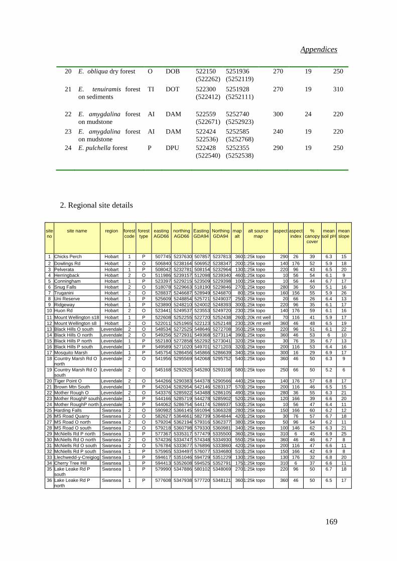
Appendices
169
20 E. obliqua dry forest O DOB 522150
(522262)
5251936
(5252119)
270 19 250
21 E. tenuiramis forest
on sediments
TI DOT 522300
(522412)
5251928
(5252111)
270 19 310
22 E. amygdalina forest
on mudstone
AI DAM 522559
(522671)
5252740
(5252923)
300 24 220
23 E. amygdalina forest
on mudstone
AI DAM 522424
522536)
5252585
(5252768)
240 19 220
24 E. pulchella forest P DPU 522428
(522540)
5252355
(5252538)
290 19 250
2. Regional site details
site no
site name
region
forest code
forest type
easting AGD66
northing AGD66
Easting GDA94
Northing GDA94
map alt
alt source
map
aspect
aspect index
%
canopy cover
mean
soil pH
mean slope
1 Chicks Perch Hobart 1 P 507745 5237630 507857 5237813 360 1:25k topo 290 26 39 6.3 15
2 Dowlings Rd Hobart 2 O 506840 5238164 506952 5238347 200 1:25k topo 140 176 52 5.9 18
3 Pelverata Hobart 1 P 508042 5232781 508154 5232964 130 1:25k topo 220 96 43 6.5 20
4 Herringback Hobart 2 O 511986 5239157 512098 5239340 460 1:25k topo 10 56 54 6.1 9
5 Conningham Hobart 1 P 523397 5229215 523509 5229398 100 1:25k topo 10 56 44 6.7 17
6 Snug Falls Hobart 2 O 518078 5229663 518190 5229846 270 1:25k topo 280 36 50 5.1 16
7 Truganini Hobart 2 O 528837 5246687 528949 5246870 80 1:25k topo 160 156 55 5.9 26
8 Uni Reserve Hobart 1 P 525609 5248854 525721 5249037 250 1:25k topo 20 66 26 6.4 13
9 Ridgeway Hobart 1 P 523890 5248210 524002 5248393 300 1:25k topo 220 96 35 6.1 17
10 Huon Rd Hobart 2 O 523441 5249537 523553 5249720 230 1:25k topo 140 176 59 6.1 16
11 Mount Wellington s18 Hobart 1 P 522608 5252255 522720 5252438 260 1:20k mt well 70 116 41 5.9 17
12 Mount Wellington s8 Hobart 2 O 522011 5251965 522123 5252148 230 1:20k mt well 360 46 48 6.5 19
13 Black Hills O south Levendale 2 O 548534 5272525 548646 5272708 350 1:25k topo 220 96 51 6.1 22
14 Black Hills O north Levendale 2 O 549256 5272931 549368 5273114 390 1:25k topo 360 46 53 6 10
15 Black Hills P north Levendale 1 P 552180 5272858 552292 5273041 320 1:25k topo 30 76 35 6.7 13
16 Black Hills P south Levendale 1 P 549589 5271020 549701 5271203 320 1:25k topo 200 116 53 6.4 16
17 Mosquito Marsh Levendale 1 P 545754 5286456 545866 5286639 340 1:25k topo 300 16 29 6.9 17
18 Country Marsh Rd O north
Levendale 2 O 541956 5295569 542068 5295752 540 1:25k topo 360 46 50 6.3 9
19 Country Marsh Rd O south
Levendale 2 O 545168 5292925 545280 5293108 580 1:25k topo 250 66 50 5.2 6
20 Tiger Point O Levendale 2 O 544266 5290383 544378 5290566 440 1:25k topo 140 176 57 6.8 17
21 Brown Mtn South Levendale 1 P 542034 5282954 542146 5283137 570 1:25k topo 200 116 46 6.5 15
22 Mother Rough O Levendale 2 O 543376 5285922 543488 5286105 490 1:25k topo 280 36 55 6.3 21
23 Mother RoughP south Levendale 1 P 544166 5285719 544278 5285902 520 1:25k topo 120 166 39 6.6 20
24 Mother RoughP north Levendale 1 P 544062 5286754 544174 5286937 530 1:25k topo 10 56 47 6.4 11
25 Harding Falls Swansea 2 O 590982 5366145 591094 5366328 280 1:25k topo 150 166 60 6.2 12
26 MS Road Quarry Swansea 2 O 582627 5364661 582739 5364844 420 1:25k topo 30 76 57 6.7 18
27 MS Road O north Swansea 2 O 579204 5362194 579316 5362377 380 1:25k topo 50 96 54 6.2 11
28 MS Road O south Swansea 2 O 579218 5360798 579330 5360981 340 1:25k topo 100 146 62 6.3 21
29 McNiells Rd P north Swansea 1 P 577367 5335317 577479 5335500 360 1:25k topo 310 6 45 6.9 25
30 McNiells Rd O north Swansea 2 O 574236 5334747 574348 5334930 550 1:25k topo 360 46 46 6.7 8
31 McNiells Rd O south Swansea 2 O 576784 5333677 576896 5333860 420 1:25k topo 200 116 47 6.6 11
32 McNiells Rd P south Swansea 1 P 575965 5334497 576077 5334680 510 1:25k topo 150 166 42 6.9 8
33 Llechwedd-y-Creigiog Swansea 1 P 594617 5351046 594729 5351229 130 1:25k topo 130 176 32 6.8 20
34 Cherry Tree Hill Swansea 1 P 594413 5352608 594525 5352791 175 1:25k topo 310 6 37 6.6 11
35 Lake Leake Rd P south
Swansea 1 P 579990 5347886 580102 5348069 270 1:25k topo 220 96 50 6.7 18
36 Lake Leake Rd P north
Swansea 1 P 577608 5347938 577720 5348121 360 1:25k topo 360 46 50 6.5 17

Appendices
170
3: Table of beetle species/morphospecies sampled
-see attached Excel file
4: Table of spider species/morphospecies sampled
-see attached Excel file
Addendum:
- A list of references used for identification of Tasmanian beetles and spiders
may be found by following this link:
https://sites.google.com/site/lynneforster/taxonomyreferences
- Some background information on the relationship between beetles and fungi
- And
- Background information on the effect of pitfall trapping and different
solutions in pitfall traps on the species sampled, may be found at the following
link:
https://sites.google.com/site/lynneforster/beetleecology

Appendices
171