Lectures on Differential Geometry

Math 240A

Fall 2014

John Douglas MooreDepartment of Mathematics

University of CaliforniaSanta Barbara, CA, USA 93106e-mail: moore@math.ucsb.edu

December 12, 2014

Preface

This is a set of lecture notes for the course Math 240A given during the Fall of2014. The notes will evolve as the course progresses. Starred sections are notfully covered in the lectures; they discuss digressions which are less central tothe core subject matter of the course.

The bibliography at the end of the notes provides some suggestions for fur-ther reading related to the topics treated in the course.

i

Contents

1 Smooth manifolds 11.1 Topological manifolds . . . . . . . . . . . . . . . . . . . . . . . . 11.2 Smooth manifolds . . . . . . . . . . . . . . . . . . . . . . . . . . 31.3 New manifolds from old . . . . . . . . . . . . . . . . . . . . . . . 121.4 The tangent space . . . . . . . . . . . . . . . . . . . . . . . . . . 171.5 The cotangent space . . . . . . . . . . . . . . . . . . . . . . . . . 211.6 The tangent and cotangent bundles . . . . . . . . . . . . . . . . . 25

2 Submanifolds 312.1 Immersions and imbeddings . . . . . . . . . . . . . . . . . . . . . 312.2 Lie groups . . . . . . . . . . . . . . . . . . . . . . . . . . . . . . . 362.3 The inverse function theorem . . . . . . . . . . . . . . . . . . . . 402.4 Whitney’s imbedding theorem . . . . . . . . . . . . . . . . . . . . 49

3 Differential equations 563.1 Vector fields and differential equations . . . . . . . . . . . . . . . 563.2 Lie bracket . . . . . . . . . . . . . . . . . . . . . . . . . . . . . . 613.3 Lie groups revisited . . . . . . . . . . . . . . . . . . . . . . . . . . 653.4 Actions of Lie groups on manifolds . . . . . . . . . . . . . . . . . 73

4 Differential forms 774.1 Tensor algebra . . . . . . . . . . . . . . . . . . . . . . . . . . . . 774.2 Exterior algebra . . . . . . . . . . . . . . . . . . . . . . . . . . . 844.3 The exterior derivative . . . . . . . . . . . . . . . . . . . . . . . . 874.4 Integration of differential forms . . . . . . . . . . . . . . . . . . . 944.5 Theorem of Stokes . . . . . . . . . . . . . . . . . . . . . . . . . . 974.6 De Rham cohomology . . . . . . . . . . . . . . . . . . . . . . . . 1014.7 The Poincare Lemma . . . . . . . . . . . . . . . . . . . . . . . . . 1064.8 Applications of de Rham theory . . . . . . . . . . . . . . . . . . . 1104.9 The Mayer-Vietoris Sequence* . . . . . . . . . . . . . . . . . . . 1124.10 The Hodge star* . . . . . . . . . . . . . . . . . . . . . . . . . . . 1174.11 Lorentz manifolds; Maxwell’s equations* . . . . . . . . . . . . . . 1214.12 The Hodge Laplacian* . . . . . . . . . . . . . . . . . . . . . . . . 125

ii

Bibliography 131

iii

Chapter 1

Smooth manifolds

Manifolds are higher dimensional generalizations of curves and surfaces in Eu-clidean space.

It is important to develop “calculus on manifolds” for many reasons. Forexample, to provide a mathematical formulation for heat flow on a surface inEuclidean space, we need a theory of partial differential equations on a curvedsurface. More generally, we need a global calculus of several variables to properlyformulate problems arising in subjects such as electricity and magnetism, fluidmechanics, classical mechanics or general relativity. Such a calculus of severalvariables extends and clarifies Stokes’s Theorem and the Divergence Theoremfrom ordinary calculus of several variables. Finally, manifolds provide an im-portant family of examples to which we can apply the techniques of topology.

1.1 Topological manifolds

The first step is the theory of topological manifolds, and for this, we needto assume some background in real analysis. Although all we really need isthe topology of metric spaces, the more general notion of topological space issometimes useful. Rudin [16] is a good reference for real analysis with far morethan we need, while Munkres [15] provides a nice introduction to point-settopology with all the key definitions and examples.

Definition. A topological space is a pair (X, T ) where X is a set and T is acollection of subsets of X such that

1. the empty set ∅ and the entire space X are both elements of T ,

2. the intersection of any two elements in T is in T , and

3. the union of an arbitrary collection of elements in T lies in T .

We say that T is a topology on X. Elements of T are called open sets. A subsetA ⊆ X is said to be closed if its complement X −A is open.

1

Key example. The example needed most for multivariable calculus is X = Rnwith the topology defined by the standard metric

d : Rn × Rn → R, with d(x,y) = |x− y|.

Using this metric, we define the ε-ball N(x; ε) about a point x ∈ X to be

N(x; ε) = y ∈ X : d(x,y) < ε.

We say that a subset U of X lies in the topology T defined by the metric d if

x ∈ U ⇒ N(x; ε) ⊆ U, for some ε > 0.

One can then check that this collection T of subsets of X satisfies all the aboveaxioms for topological space. For each x ∈ Rn and each ε > 0, N(x; ε) is open,and we call N(x; ε) an open ball about x of radius ε. We say that the T wehave just constructed is the standard topology on Rn.

Another example. Suppose that X is a subset of Rn. In this case, we can letT be the collection of subsets of X such that

U ∈ T ⇔ U = V ∩X, where V is open in Rn.

Then T is the subspace topology that X inherits from Rn.

Definition. Suppose that (X1, T1) and (X2, T2) are topological spaces. Afunction f : X1 → X2 is continuous if

U2 ∈ T2 ⇒ f−1(U2) ∈ T1.

In other words, a function f : X1 → X2 is continuous if the inverse image ofany open set in X2 is open in X1. A function f : X1 → X2 is said to be ahomeomorphism if it is a continuous bijection which has a continuous inversef−1 : X2 → X1.

A topologist would regard two topological spaces (X1, T1) and (X2, T2) as essen-tially the same if there is a homeomorphism from (X1, T1) to (X2, T2). One ofthe fundamental problems of topology would be to classify all topological spacesup to homeomorphism, but it is impossibly difficult. We are more interested inunderstanding those topological spaces on which one could do calculus. Thereare two additional axioms of a somewhat technical nature that we will imposeto exclude pathological topological spaces.

Definition. A topological space (X, T ) is Hausdorff if whenever p and q aredistinct elements of X, there exist elements U, V ∈ T such that

p ∈ U, q ∈ V, U ∩ V = ∅.

Note that Rn with its standard topology is Hausdorff. Indeed, if x and y aredistinct elements of Rn, we can set ε = d(x,y). If

U = N(x; ε/3) and V = N(y; ε/3).

2

Then

x ∈ N(x; ε/3), y ∈ N(y; ε/3), N(x; ε/3) ∩N(y; ε/3) = ∅,

and hence Rn with its standard topology is indeed Hausdorff.

Definition. Suppose that (X, T ) is a topological space. A subset B ⊆ T isa countable base for T if B is countable and every element of T is a union ofelements of B. If the topological space (X, T ) has a countable base, it is said tobe second countable.

In the case of Rn with its standard topology, we can let B be the set of openballs

N((r1, r2, . . . , rn), ε) such that r1, r2, . . . , rn, ε ∈ Q.

then B is countable and one can check that any open set is a union of elementsof B. Thus Rn with its standard topology is second countable.

It is easy to verify that any subspace of Rn with the subspace topology isalso Hausdorff and second countable.

Definition. An n-dimensional topological manifold is a Hausdorff second count-able topological space (M, T ) such that every point p ∈ M lies in an open setwhich is homeomorphic to an open subset of Rn with the topology induced fromthe standard topology on Rn.

Alternatively, we can say that M is a topological manifold of dimension n.

1.2 Smooth manifolds

Here is some additional useful terminology for topological manifolds: A chart orcoordinate system on an n-dimensional topological manifold M is a pair (U, φ),where U is an open subset of M and φ is a homeomorphism from U onto anopen subset φ(U) of Rn.

An atlas A on M is a collection A = (Uα, φα) : α ∈ A of charts on Msuch that ⋃

Uα : α ∈ A = M.

We say that an atlas A = (Uα, φα) : α ∈ A on M is smooth if

φβ φ−1α : φα(Uα ∩ Uβ) −→ φβ(Uα ∩ Uβ)

is smooth (that is, C∞) for every choice of α, β ∈ A. Two smooth atlases Aand B on M are said to be equivalent if A ∪ B is a smooth atlas.

Definition. An n-dimensional smooth manifold or a smooth manifold of dimen-sion n is an n-dimensional topological manifold together with an equivalenceclass of smooth atlases.

3

Suppose now that M and N are smooth manifolds of possibly different dimen-sions) with smooth atlases A = (Uα, φα) : α ∈ A and B = (Vβ , φβ) : β ∈ Brespectively. Then a function F : M → N is said to be smooth if

ψβ F φ−1α : φα(Uα ∩ F−1(Vβ)) −→ ψβ(Vβ)

is smooth for each α ∈ A and each β ∈ B.Note that the identity map id : M → M from a manifold to itself is a

smooth map, and that if F : M → N and G : N → P are smooth mapsbetween smooth manifolds, then so is the composition G F : M → P . Wesay smooth manifolds and maps form a “category” with the “objects” being thesmooth manifolds and the “morphisms” being smooth maps. A smooth functionF : M → N is a diffeomorphism if it is a bijection and its inverse F−1 : N →Mis smooth. Two diffeomorphic manifolds are often regarded as “the same” fromthe point of view of differential topology.

Example 1. The simplest example of an n-dimensional smooth manifold is Rn.In this case, we can take the atlas to consist of a single element, A = (Rn, id),where id denotes the identity map on Rn. Any open subset of Rn is also asmooth manifold.

Two-dimensional smooth manifolds are also called smooth surfaces, and the firstrigorous definition of smooth manifold seems to have occurred within Weyl’streatment of the theory of Riemann surfaces, a key example of which is theRiemann sphere:

Example 2. The Riemann sphere, can be thought of intuitively as the spaceobtained from the complex plane C by adding a point at infinity, a point whichwe denote by ∞. To be more rigorous, we regard it as the unit sphere

S2 = (x1, x2, x3) ∈ R3 : (x1)2 + (x2)2 + (x3)2 = 1,

and give it the topology that it inherits as a subspace of R3. With the subspacetopology, it is Hausdorff and second countable and we will shortly see that it isalso a topological manifold. In fact, we will construct charts on the Riemannsphere via stereographic projection.

If N = (0, 0, 1) is the north pole on S2, stereographic projection is a one-to-one onto function

Φ : C −→ S2 − N,

where C is thought of as the (x1, x2)-plane in R3. It is constructed by consideringthe line L containing N = (0, 0, 1) on S2 and the point (x, y, 0) in the planex3 = 0. This line L can be parametrized by

γ : R→ R3 where γ(t) = (x1(t), x2(t), x3(t)) = t(x, y, 0) + (1− t)(0, 0, 1).

Alternatively, we can write this as

x1(t) = tx, x2(t) = ty, x3(t) = 1− t. (1.1)

4

There is a unique nonzero value for t such that γ(t) lies on S2 − N, and itoccurs when

1 = (x1)2 + (x2)2 + (x3)2 = t2x2 + t2y2 + (1− t)2.

We can expand and solve for t:

1 = t2(x2 + y2) + 1− 2t+ t2 = t2(x2 + y2 + 1)− 2t+ 1,

2t = t2(x2 + y2 + 1), 2 = t(x2 + y2 + 1), t =2

x2 + y2 + 1.

Substitution into (1.1) then yields the point on S2 which corresponds to thepoint (x, y, 0), corresponding to x+ iy ∈ C:

x1 =2x

x2 + y2 + 1, x2 =

2y

x2 + y2 + 1, x3 = 1− 2

x2 + y2 + 1.

We can then simplify this to

x1 =2x

x2 + y2 + 1, x2 =

2y

x2 + y2 + 1, x3 =

x2 + y2 − 1

x2 + y2 + 1, (1.2)

which gives an explicit formula for stereographic projection

Φ : C −→ S2 − N, Φ(z) =

(2Re(z)

|z|2 + 1,

2Im(z)

|z|2 + 1,|z|2 − 1

|z|2 + 1

),

where Re(z) and Im(z) are the real and imaginary parts of z = x+ iy.To see that Φ is one-to-one and onto, we can construct an explicit inverse.

Indeed, eliminating t from equations (1.1) gives first t = 1− x3 and then

x =x1

t=

x1

1− x3, y =

x2

t=

x2

1− x3.

Thus we can set U = S2 − N and define a function

φ : U −→ C by φ(x1, x2, x3) =x1 + ix2

1− x3. (1.3)

which is exactly the inverse of Φ. The inverse map φ is well-behaved exceptwhen x3 = 1, that is, it is well-behaved except at the north pole N on S2.

These explicit formulae may seem confusing at first. The important pointto note is that as the modulus of z gets larger and larger, Φ(z) approaches thenorth pole on S2. Thus if we think of using Φ to identify points of C with pointson S2−N, then the north pole N should be identified with a point at infinity.Indeed we might think of extending Φ to a map

Φ : C ∪ ∞ −→ S2

5

which takes∞ to the north pole N . This idea of adding a point at infinity to thecomplex plane, thereby obtaining what is sometimes called the extended complexplane or the one-point compactification of C, has turned out to be extremelyuseful in understanding functions of a complex variable.

On the other hand, we can think of (U, φ) as defining a chart or a coordinatez on S2, which is well-behaved everywhere except at the north pole N . Butsometimes we want a coordinate w that is well-behaved near ∞, and we mighttry to take

w =1

z

as such a coordinate. Can we think of this also as a coordinate on part of S2?We find that

z =x1 + ix2

1− x3⇒ w =

1

z=

1− x3

x1 + ix2=

(1− x3)(x1 − ix2)

(x1)2 + (x2)2

=(1− x3)(x1 − ix2)

1− (x3)2=x1 − ix2

1 + x3

Thus if we let S denote the south pole (0, 0,−1), set V = S2 − S and define

ψ : V −→ C by w = ψ(x1, x2, x3) =x1 − ix2

1 + x3. (1.4)

It is relatively easy to show that conjugation followed by the inverse of ψ is juststereographic projection with the north pole replaced by the south pole.

We now have two charts (U, φ) and (V, ψ) defined by (1.3) and (1.4),

φ : S2 − N → C and ψ : S2 − S → C,

which are related by

ψ φ−1(z) = w =1

zand φ ψ−1(w) = z =

1

w, (1.5)

or

ψ φ−1(u1, u2) =(u1,−u2)

(u1)2 + (u2)2and φ ψ−1(v1, v2) =

(v1,−v2)

(v1)2 + (v2)2.

These formulae show that

A = (U, φ), (V, ψ)

form a smooth atlas on S2, which make it into a smooth two-dimensional man-ifold.

The Riemann sphere is more than just a two-dimensional smooth manifold.Indeed, the transformation formulae (1.5) make S2 into what is called a Riemannsurface, in accordance with the definition we next give.

6

We say that an atlas A = (Uα, φα) : α ∈ A on a two-dimensional topolog-ical manifold M is holomorphic if the charts (Uα, φα) in the atlas take values inthe complex plane C (which of course is homeomorphic to R2) and

φβ φ−1α : φα(Uα ∩ Uβ) −→ φβ(Uα ∩ Uβ)

is holomorphic for every choice of α, β ∈ A. Two holomorphic atlases A and Bon M are said to be equivalent if A ∪ B is a holomorphic atlas. We can thenmodify the definition of smooth manifold:

Definition. A Riemann surface is a two-dimensional topological manifold to-gether with an equivalence class of holomorphic atlases.

The transformation formulae (1.5) show that the atlas A = (U, φ), (V, ψ) wejust constructed on S2 is a holomorphic atlas, which makes S2 into a Riemannsurface.

Suppose that Σ1 and Σ2 are Riemann surfaces with holomorphic atlasesA = (Uα, φα) : α ∈ A and B = (Vβ , φβ) : β ∈ B respectively. Then afunction F : Σ1 → Σ2 is said to be holomorphic if

ψβ F φ−1α : φα(Uα ∩ F−1(Vβ)) −→ ψβ(Vβ)

is holomorphic for each α ∈ A and each β ∈ B. A holomorphic functionF : Σ1 → Σ2 is a holomorphic diffeomorphism if it is a bijection and its inverseF−1 : N →M is also holomorphic. One of the goals or Riemann surface theoryis to classify Riemann surfaces up to holomorphic diffeomorphism.

Digression. The notion of Riemann surfaces makes it much easier to developthe properties of rational functions in complex analysis. Recall that a rationalfunction is simply a complex-valued function of the form

f(z) =P (z)

Q(z), (1.6)

where

P (z) = amzm + am−1z

m−1 + · · ·+ a1z + a0

and Q(z) = bnzn + bn−1z

n−1 + · · ·+ b1z + b0

are polynomials with complex coefficients

am, am−1, . . . , a1, a0, bn, bn−1, . . . , b1, b0,

and we make the assumptions that am 6= 0 and bn 6= 0, and that P and Q do nothave any common factors. In ordinary complex analysis, the function f wouldonly be defined on

C− zeros of Q ,

but the properties of such a rational functions are far clearer when it is con-sidered to be a holomorphic function F : S2 → S2, where S2 is the Riemann

7

sphere, with F (z) = ∞, when P (z) = 0. In particular, the linear fractionaltransformations T defined by

T (z) =az + b

cz + d,

where a, b, c and d are complex numbers such that ad − bc 6= 0, extend toholomorphic diffeomorphisms T : S2 → S2, the inverse of T given by

T−1(z) =dz − b−cz + a

,

as one verifies by a direct calculation. Moreover, the composition of two linearfractional transformations is another linear fractional transformation, the linearfractional transformations forming a group under composition.

Although the definition of Riemann surface is similar to that of a two-dimensional smooth manifold, the theory of Riemann surfaces is far more rigid.Indeed, we will see later that there are many, many smooth diffeomorphismsof S2, while the only holomorphic diffeomorphisms of S2 are the linear frac-tional transformations. To prove the latter fact, we need some results fromcomplex analysis. First note that we can assume without loss of generality thatF (∞) =∞, since we can arrange this after composition with a linear fractionaltransformation. But then F restricts to a holomorphic diffeomorphism of C,which we also denote by F . It then follows from Theorem 3.3, Chapter 5 ofLang [8] (which is based upon a theorem of Weierstrass regarding essential sin-gularities) that F (z) = az + b, for some complex numbers a and b. But this isexactly the form of a linear fractional transformation which takes ∞ to ∞.

More details on the theory of Riemann surfaces can be found in many ex-cellent books on this subject, including the highly recommended reference byForster [5].

We can extend our proof that S2 has a smooth manifold to n dimensions:

Example 3. We let

Sn = (x1, x2, . . . , xn+1) ∈ Rn+1 : (x1)2 + (x2)2 + · · ·+ (xn+1)2 = 1,

with the topology it inherits as a subspace of Rn+1, which is automaticallyHausdorff and second countable. We can extend the construction of the chartsmade in Example 2 and perhaps make the computations a little more efficient.Thus we let N = (0, 0, . . . , 1) be the north pole in Rn+1, let S = (0, 0, . . . ,−1)be the south pole, and consider the two open sets

U = Sn − N, V = Sn − S.

We claim that there are bijections

φ : U −→ Rn, ψ : V −→ Rn

such thatA = (U, φ), (V, ψ)

8

is a smooth atlas on Sn which makes it into an n-dimensional smooth manifold.Of course, the construction is the same as in the preceding example, namely

we let φ be the inverse of stereographic projection from the north pole,

φ(x1, x2, . . . , xn+1) = (u1, u2, . . . un),

where

(u1, u2, . . . un, 0) = (0, 0, . . . , 1) + λ((x1, x2, . . . , xn+1)− (0, 0, . . . , 1)

).

Then

0 = 1 + λ(xn+1 − 1) ⇒ λ =1

1− xn+1,

so

φ(x1, x2, . . . , xn+1) = u = (u1, u2, . . . un) =1

1− xn+1(x1, x2, . . . xn). (1.7)

Thus

|u|2 = u · u =(x1)2 + (x2)2 + · · ·+ (xn)2

(1− xn+1)2=

1− (xn+1)2

(1− xn+1)2=

1 + xn+1

1− xn+1.

We can now solve for xn+1, and obtain

|u|2 + 1 =2

1− xn+1, |u|2 − 1 =

2xn+1

1− xn+1, xn+1 =

|u|2 − 1

|u|2 + 1.

It follows that

(x1, x2, . . . , xn) = (1− xn+1)(u1, u2, . . . un) =2

|u|2 + 1(u1, u2, . . . un),

and

φ−1(u1, u2, . . . un) = (x1, x2, . . . , xn+1) =1

|u|2 + 1(2u1, 2u2, . . . 2un, |u|2 − 1).

(1.8)Formulae (1.7) and (1.8) show that φ is a homeomorphism from U to Rn.

Similarly, we define ψ : V → Rn to be the inverse of stereographic projectionfrom the south pole,

ψ(x1, x2, . . . , xn+1) = (v1, v2, . . . vn),

where

(v1, v2, . . . vn, 0) = (0, 0, . . . ,−1) + λ((x1, x2, . . . , xn+1)− (0, 0, . . . ,−1)

).

The only thing that changes is the sign of xn+1 in the preceding formulae, sothe same argument shows that ψ is a diffeomorphism, and

(v1, v2, . . . vn) = ψ(x1, x2, . . . , xn+1) =1

1 + xn+1(x1, x2, . . . xn).

9

It follows that

(x1, x2, . . . , xn) = (1− xn+1)(u1, u2, . . . un) = (1 + xn+1)(v1, v2, . . . vn),

so

ψ φ−1(u1, u2, . . . un) =1− xn+1

1 + xn+1(u1, u2, . . . , un) =

1

|u|2(u1, u2, . . . , un). (1.9)

Similarly,

φ ψ−1(v1, v2, . . . vn) =1

|v|2(v1, v2, . . . , vn),

so we see that (U, φ), (V, ψ) is a smooth atlas on Sn.As long as we’re not worried about questions of orientation, the atlas we

have constructed is perfectly fine, but it turns out that the coordinate change(1.9) which simply simply inverts a point through the unit sphere in Rn reversesorientation (because it reverses the direction of the radial coordinate). We canrepair this small defect in our atlas by replacing ψ by ψ = R ψ, where

R : Rn → Rn by R(v1, . . . , vn−1, vn) = (v1, . . . , vn−1,−vn).

If we make this small change and specialize to the case n = 2, we recover thesame atlas A = (U, φ), (V, ψ) as in Example 2.

We can modify the defintion of a smooth manifold slightly to get the defini-tion of an oriented manifold. Suppose that

φα = (x1, . . . , xn) : Uα → Rn, φβ = (y1, . . . , yn) : Uβ → Rn

are two charts on an n-dimensional topological manifold M . On the overlapφα(Uα ∩ Uβ), we can define the Jacobian matrix

D(φβ φ−1α ) =

∂y1/∂x1 · · · ∂y1/∂xn

· · · · ·∂yn/∂x1 · · · ∂yn/∂xn

: φα(Uα ∩ Uβ)→ GL(n,R),

where GL(n,R) is the space of invertible n×n matrices. We say that the charts(Uα, φα) and (Uβ , φβ) are coherently oriented if

det(D(φβ φ−1α )) : φα(Uα ∩ Uβ) −→ R− 0

is positive. We say that a smooth atlas A = (Uα, φα) : α ∈ A on M is orientedif (Uα, φα) and (Uβ , φβ) are coherently oriented for every choice of α, β ∈ A.Two oriented smooth atlases A and B on M are said to be equivalent if A ∪ Bis an oriented smooth atlas.

Definition. An oriented smooth n-dimensional manifold is an n-dimensionalsmooth manifold with an equivalence class of oriented smooth atlases.

Thus for example, the atlas (U, φ), (V, ψ) we constructed above on Sn makesit into an oriented smooth n-dimensional manifold.

10

Exercise I. (Due Monday, October 13.) Let RPn be the set of all lines whichpass through the origin in Rn+1. More precisely, we define an equivalence rela-tion ∼ on Rn+1 − (0, 0, . . . , 0) by

(x1, x2, . . . , xn+1) ∼ (y1, y2, . . . , yn+1)

if and only if there exists λ ∈ R− 0 such that

(x1, x2, . . . , xn+1) = λ(y1, y2, . . . , yn+1),

and we let [x1, x2, . . . xn+1] denote the equivalence class of (x1, x2, . . . , xn+1).We can identify [x1, x2, . . . xn+1] with the line passing through (0, 0, . . . , 0) and(x1, x2, . . . , xn+1), and thus RPn is simply the quotient space

RPn =Rn+1 − (0, 0, . . . , 0)

∼,

and we let π : Rn+1 − (0, 0, . . . , 0) → RPn denote the quotient map. (Alter-natively, we can restrict the projection π to Sn ⊆ Rn+1 − (0, 0, . . . , 0) andregard RPn as a quotient of Sn with a projection π : Sn → RPn that identifiesantipodal points.)

We give RPn the quotient topology it inherits from Rn+1 − (0, 0, . . . , 0).Thus a subset U lies in TRPn if and only if π−1(U) is open in Rn+1−(0, 0, . . . , 0).Show that this topology is Hausdorff and has a countable base. For 1 ≤ i ≤ n+1,let

Ui = [x1, x2, . . . xn+1] ∈ RPn : xi 6= 0

and define φi : Ui → Rn by

φi([x1, x2, . . . xn+1]) =

(x1

xi, . . . ,

xi−1

xi,xi+1

xi, . . . ,

xn+1

xi

)Show that A = (Ui, φi) : 1 ≤ i ≤ n+1 is a smooth atlas on RPn which makesRPn into an n-dimensional smooth manifold.

Dangerous curve. This atlas we have constructed on RPn is not orientedwhen n is even. In fact, we will see later in the course that there is no orientedatlas on RPn when n is even, and in this case we say that RPn is a nonorientablesmooth manifold of dimension n.

Exercise IA. (Do not hand in.) Let CPn be the set of all lines which passthrough the origin in Cn+1. As in the previous exercise, we define an equivalencerelation ∼ on Cn+1 − (0, 0, . . . , 0) by

(z1, z2, . . . , zn+1) ∼ (w1, w2, . . . , wn+1)

if and only if there exists λ ∈ C− 0 such that

(z1, z2, . . . , zn+1) = λ(w1, w2, . . . , wn+1),

11

and we let [z1, z2, . . . zn+1] denote the equivalence class of (z1, z2, . . . , zn+1). Weidentify [z1, z2, . . . zn+1] with the line passing through the points (0, 0, . . . , 0) and(z1, z2, . . . , zn+1), which identifies CPn with the quotient space

CPn =Cn+1 − (0, 0, . . . , 0)

∼.

Show that CPn is a smooth manifold of dimension 2n. Can you show that CP 1

is diffeomorphic to S2?

1.3 New manifolds from old

We can construct new manifolds from old by taking products or connectedsums. Before describing how to do this, we introduce some terminology. If Mis a smooth manifold with smooth atlas A = (Uα, φα) : α ∈ A, we say that achart (U, φ) on M is smooth if

φ φ−1α and φα φ−1 are smooth where defined,

for all α ∈ A. If p ∈ M , there always exists a smooth chart (U, φ) such thatp ∈ U and φ(p) = 0.

There is one really easy way of constructing new manifolds. Note that if Mis a smooth manifold of dimension n with smooth atlas A = (Uα, φα) : α ∈ Aand U is an open subset of M , we can make U into a smooth manifold ofdimension n by giving U the subspace topology and the atlas

A ∩ U = (Uα ∩ U, φα|(Uα ∩ U)) : α ∈ A.

Thus any open subset of a smooth manifold is a smooth manifold in its ownright.

Products of manifolds: Suppose that M and N are smooth manifolds ofdimensions m and n respectively, and suppose that M and N have smoothatlases A = (Uα, φα) : α ∈ A and B = (Vβ , φβ) : β ∈ B respectively.We claim that we can then make the Cartesian product M ×N into a smoothmanifold of dimension m+ n.

First, if TM and TN are the topologies on M and N respectively, we can set

BM×N = U × V ⊆M ×N : U ∈ TM , V ∈ TN.

We then let TM×N be the collection of all unions of elements of BM×N . It isstraightforward to check that TM×N is a topology on M × N , and we call itthe product topology . It is also not difficult to check that (M × N, TM×N ) isHausdorff and has a countable base for its topology.

As a smooth atlas on M ×N , we take the product atlas

A× B = (Uα × Vβ , φα × ψβ) : α ∈ A, β ∈ B.

12

Note thatφα × ψβ : Uα × Vβ −→ Rm+n.

It is straightforward to check that the resulting atlas is smooth. Moreover, if Aand B are oriented smooth atlases, so is the product A× B.

For example, we could take M = Sm and N = Sn, each with the atlasdescribed in the previous section. The product atlas on Sm × Sn has fourelements. We can always enlarge our atlas by including an arbitrary number ofnew smooth charts without changing the equivalence class of the atlas.

Quotients: Let Diff(M) denote the set of diffeomorphisms from a smoothmanifold M to itself, a group under composition. Suppose that Γ is a subgroupof Diff(M).

We say that Γ acts freely on M if the only γ ∈ Γ which leaves any point ofM fixed is the identity. We say that Γ acts properly discontinuously on M ifevery p ∈M has an open neighborhood U such that

γ ∈ Γ : γ(U) ∩ U 6= ∅ is finite.

If Γ acts freely and properly discontinuously on M , then every p ∈ M has anopen neighborhood U such that

γ ∈ Γ : γ(U) ∩ U 6= ∅ = id. (1.10)

If Γ acts freely and properly discontinuously on M , we let M/Γ be the spaceof orbits, the space of equivalnece classes of points of M under the equivalencerelation

p ∼ q ⇔ there exists γ ∈ Γ such that γ(p) = q.

We let π : M → M/Γ be the projection which takes p to the equivalence class[p] of p, and given M/Γ the quotient topology which declares a set U ⊆ M/Γto be open if and only if π−1(U) is open in M .

Proposition 1.3.1. If Γ is a group of diffeomorphisms which acts freely andproperly discontinuously on a smooth n-dimensional manifold M , then M/Γ isa smooth n-dimensional manifold in such a way that π : M →M/Γ is a smoothlocal diffeomorphism.

(By saying that π is a local diffeomorphism, we mean that any p ∈ M has anopen neighborhood U such that π|U is a diffeomorphism.)

Sketch of proof: We leave it to the reader to check that the quotient topologyon M/Γ is Hausdorff and second countable. We need to construct the smoothcharts on M/Γ. For a given choice of p ∈M , we let (Up, φp) be a smooth charton M with p ∈ Up such that Up satisfies condition (1.10). Then π maps Uphomeomorphically onto π(Up) ⊆M/Γ. Hence

(Vpψp) = (π(Up), φp (π|Up)−1)

13

is a chart on M/Γ. Finally, we check that

(Vp, ψp) : p ∈M

is a smooth atlas on M/Γ making it into a smooth n-dimensional manifold withthe required properties.

For example, suppose that M = R2 and that Γ is the free abelian group gener-ated by the translations

τ1 : R2 → R2, τ1(x, y) = (x+ 1, y),

τ2 : R2 → R2, τ1(x, y) = (x+ u, y + v),

where (u, v) ∈ R2 and v > 0. Then Γ is a subgroup of Diff(Rn) and

R2/Γ = T 2 = torus.

Connected sums of manifolds: If M and N are smooth manifolds of di-mension n, we can construct a new manifold M]N of dimension n, called theconnected sum of M and N by taking disks out of M and N and identifying theresults along the boundaries of the disks. If M and N are oriented manifolds,the connected sum will also be oriented.

Here is a more detailed description of the construction: Suppose that p ∈Mand q ∈ N , and that we have chosen charts

(U, φ) = (U, (x1, . . . , xn)) on M such that p ∈ U and φ(p) = 0,

and

(V, ψ) = (V, (y1, . . . , yn)) on N such that q ∈ V and ψ(q) = 0.

We letBε(0) = x ∈ Rn : |x| < ε, Bε(0) = x ∈ Rn : |x| ≤ ε

and suppose that

B2(0) ⊂ φ(U) and B2(0) ⊂ ψ(V ),

by rescaling the coordinates if necessary. We suppose that M and N have atlases

A = (Uα, φα) : α ∈ A ∪ (U, φ), B = (Vβ , φβ) : β ∈ B ∪ (V, ψ)

such that for each α ∈ A and β ∈ B,

Uα ∩ φ−1(B1/2(0)) = ∅, Vβ ∩ ψ−1(B1/2(0)) = ∅

and⋃Uα : α ∈ A ∪ φ−1(B2(0)) = m,

⋃Vβ : β ∈ B ∪ φ−1(B2(0)) = N.

14

We then define

η : B2(0)− B1/2(0) −→ B2(0)− B1/2(0) by η(x) =x

|x|2.

Note that η is simply an inversion in the sphere

Sn−1 = x ∈ Rn : |x| = 1,

which is a diffeomorphism of B2(0) − B1/2(0). Although it is orientation-reversing, if we let

R : Rn → Rn by R(x1, . . . , xn−1, xn) = (x1, . . . , xn−1,−xn),

then R η will be orientation-preserving. We set

M = M − φ−1(B1/2(0)), N = N − ψ−1(B1/2(0)),

and define an equivalence relation ∼ on the disjoint union of M and N bydecreeing that r ∈ φ−1(B2(0))∩ M is equivalent to s ∈ ψ−1(B2(0))∩ N (whichwe write as r ∼ s) if and only if

φ(r) = R η ψ(s).

Finally, we denote the set of equivalence classes by M]N .There is a unique topology on M]N which makes the inclusions

M ⊆M]N and N ⊆M]N

homeomorphisms onto open subsets. One checks once again that this topologyis Hausdorff and second countable. Note that in M]N , φ−1(B2(0)) ∩ M andψ−1(B2(0)) ∩ N are identified to a set W which is open for this topology, andwe can define

χ : W −→ Rn by χ([r]) = φ(r),

where [r] is the equivalence class of r ∈ U ∩ M . Finally, we give M]N the atlas

(Uα, φα) : α ∈ A ∪ (Vβ , R φβ) : β ∈ B ∪ (W,χ),

and check that it is smooth. This gives M]N the unique smooth manifoldstructure such that the inclusions

M ⊆M]N and N ⊆M]N

are diffeomorphisms onto open subsets of M]N , and finishes our constructionof M]N .

Note that the connected sum of two oriented manifolds of dimension n is alsooriented. The notions of product and connected sum are sufficient to enable usto describe the well-known classification of compact path connected surfaces.We first recall the definitions from topology, a subject treated in [15]:

15

Definition. A topological space (X, T ) is compact if every open cover of X hasa finite subcover.

The Heine-Borel theorem from real analysis states that a subspace of Rn withthe subspace topology is compact if and only if it is closed and bounded.

Definition. A topological space (X, T ) is said to be path connected if wheneverp and q are points of X, there is a continuous map

γ : [0, 1]→ X such that γ(0) = p and γ(1) = q.

More generally, we say that (X, T ) is connected if the only subsets of X whichare both open and closed are ∅ and X itself. In topology courses, it is shownthat path connected spaces are also connected, and for topological manifolds, itcan be shown that connectedness is equivalent to path connectedness.

It can be proven that any one-dimensional path connected smooth manifoldis diffeomorphic to either R or S1; a proof of this fact is given in the appendixto a highly recommended short book by Milnor [12].

There is also a simple classification of oriented compact path connected two-dimensional manifolds up to diffeomorphism in terms of the genus g ∈ 0 ∪n.We start with the sphere S2, which is said to have genus zero and the torusS1×S1 which has genus one. There is then a unique oriented compact connectedsurface of each genus g when g > 1, which is the connected sum of g copies ofthe torus S1 × S1.

There is also a series of nonorientable compact path connected two-dimensionalmanifolds, the connected sum of h copies of RP 2 where h ≥ 1.

Definition. A topological space (X, T ) is simply connected if it is path con-nected, and if every continuous loop

γ : [0, 1]→M, wth γ(0) = p = γ(1)

can be continuously contracted to a point. That means that there is a continuousmap H : [0, 1]× [0, 1]→M such that

H(t, 0) = H(0, u) = H(1, u) = p, H(t, 1) = γ(t).

(We can think of H as defining a family of loops γu at p by γu(t) = H(t, u)such that γ0 is a constant and γ1 = γ.)

The only compact simply connected two-dimensional manifold is S2.One can ask for classification of higher-dimensional manifolds. Work on these

topics forms the subject of more advanced courses in geometry and topology.One of the first problems considered by Poincare in the development of what

he called “analysis situs” concerned the classification of three-dimensional man-ifolds. Indeed, Poincare raised the following question in 1904 which came tobe known as the Poincare conjecture: Is any compact simply connected three-dimensional topological manifold homeomorphic to S3? During the twentieth

16

century this was regarded as one of the most important open problems in math-ematics, and it became one of the seven Clay Mathematics Institute MillenniumPrize problems for which a million dollar prize was offered in 2000. The Poincareconjecture was settled by Grigory Perelman in 2002-03. Perelman went on toprove Thurston’s geometrization conjecture, which provides a classification forthree-dimensional manifolds in terms of geometric structures on those mani-folds. Crucial to the solution were techniques for studying a nonlinear versionof the heat equation, a nonlinear partial differential equation applied to Rie-mannian metrics on three-manifolds which studied the evolution of the metricunder “Ricci flow,” as developed by Richard Hamilton. (An introductory surveyon Perelman’s work can be found in [1].)

It turns out that every topological manifold of dimension less than or equal tothree has a unique smooth manifold structure, so the classification of topologicalmanifolds of dimension ≤ 3 is the same as that for smooth manifolds.

In contrast, classification of four-dimensional manifolds is still in a fragmen-tary state. An additional complication is that although very three-dimensionaltopological manifold has a unique smooth manifold structure, in dimension fourthere is a divergence between the topological and smooth classifications. Forexample, breakthroughs of Freedman and Donaldson showed that there are un-countably many ways of making R4 into a smooth manifold—this is the onlydimension in which this can happen. Many examples are known of compactsimply connected four-dimensional topological manifolds which have no smoothstructures, and others which have infinitely many. (On the other hand, it isnot known whether the smooth four-dimensional Poincare conjecture is true:this conjecture states that the topological four-sphere S4 has only one smoothstructure.) Once again, partial differential equations on manifolds provide an es-sential technique for proving these results, this time the Yang-Mills and Seiberg-Witten equations that come from mathematical physics.

These results reverse the usual direction of application. Ordinarily one wouldthink of topology and geometry as forming a foundation for partial differentialequations and mathematical physics. It is remarkable that many of the mostimportant ideas within the topology of low-dimensional manifolds obtained inrecent years have gone in the reverse direction.

The reader can find many further examples of smooth manifolds in Chapter1 of Lee [10].

1.4 The tangent space

Our next goal is to define the various concepts from several variable calculus in amanner which does not make explicit use of local coordinates, insofar as possible.We start off with differentiation, with the notion of directional derivative at apoint, which is encapsulated in the definition of tangent vector.

A tangent vector might represent the instantaneous velocity of a particlemoving in a smooth manifold. The problem is that once we leave the comfortof Euclidean space, there is no preferred coordinate system in which to measure

17

the components of a vector—all coordinate systems are on the same footing.Tangent vectors must be defined so that their components can be allowed tochange from coordinate system to coordinate system.

Suppose that M is a smooth manifold and p ∈ M , and that F(p) denotesthe space of pairs (U, f) where U is an open subset of M containing p andf : U → R is a smooth real-valued function. For simplicity of notation, we willusually leave out the open set U and simply write f for a typical element ofF(p). We can define an equivalence relation ∼ on F(p) by

f ∼ g ⇔ f ≡ g on some open neighborhood of p.

The equivalence class of an element f ∈ F(p) is then called the germ of f at p.One can check that the space of germs is a commutative R-algebra.

Definition. A tangent vector at p ∈ M is a function v : F(p) → R whichsatisfies the following axioms:

1. v(f) = v(g) if f ≡ g on some open neighborhood of p, that is, v(f)depends only on the germ of f at p.

2. v(cf + g) = cv(f) + v(g), for f, g ∈ F(p) and c ∈ R.

3. v(fg) = f(p)v(g) + g(p)v(f), for f, g ∈ F(p).

We let TpM denote the collection of tangent vectors to M at p and call it thetangent space to M at p.

In axioms 2 and 3, if f is defined on U while g is defined on V , we regard cf + gand fg as defined on U ∩ V . The third axiom is known as the Leibniz rule fordifferentiation. It is easily verified that TpM is a real vector space.

Examples. Suppose that M is an n-dimensional smooth manifold, p ∈M , andthat

φ = (x1, . . . , xn) : U → Rn

is a smooth coordinate system on M with p ∈ U . If f ∈ F(p), we then define

∂

∂xi

∣∣∣∣p

(f) = Di(f φ−1)(φ(p)) ∈ R,

where Di denotes differentiation with respect to the i-th coordinate direction inthe Euclidean space Rn. The local coordinates therefore provide a collection of“directional derivative operators” which clearly depends only on the germ of fat p,

f ≡ g on some neighborhood of p ⇒ ∂

∂xi

∣∣∣∣p

(f) =∂

∂xi

∣∣∣∣p

(g).

One readily verifies that each of these directional derivative operators satisfiesthe other two axioms, and the Leibniz rule,

∂

∂xi

∣∣∣∣p

(fg) =

(∂

∂xi

∣∣∣∣p

(f)

)g(p) + f(p)

(∂

∂xi

∣∣∣∣p

(g)

),

18

reflects a familiar property of differentiation in Euclidean space. Hence eachdirectional derivative operator

∂

∂xi

∣∣∣∣.

is an element of the tangent space TpM . Moreover, each linear combination

n∑i=1

ai∂

∂xi

∣∣∣∣p

lies within the tangent space TpM . We will see shortly that these are the onlyelements of TpM , so that (

∂

∂x1

∣∣∣∣p

, . . . ,∂

∂xn

∣∣∣∣p

)

is a basis for the tangent space TpM . Indeed, this follows from:

Theorem 1.4.1. Suppose that M is a smooth n-dimensional manifold, thatp ∈ M and that (U, φ) = (U, (x1, . . . , xn) is a smooth chart on M with p ∈ U .If v ∈ TpM , then

v =

n∑i=1

v(xi)∂

∂xi

∣∣∣∣p

. (1.11)

To prove this, we first make the simplifying assumption that φ(p) = 0 and thatV = φ(U) is a convex subset of Rn. Our proof is based upon a series of lemmas.

Lemma 1. If v ∈ TpM and c is a constant function, then v(c) = 0.

By axiom 2 for tangent vectors,

v(1) = v(1 · 1) = 1v(1) + 1v(1), so v(1) = 2v(1) or v(1) = 0.

It then follows from axiom 1 that v(c) = cv(1) = 0. QED

Before stating the next lemma, we agree to let (x1, . . . , xn) denote the standardEuclidean coordinate system on Rn.

Lemma 2. If V is a convex neighborhood of 0 ∈ Rn and f : V → R is a C∞

function, then there are C∞ functions g1, . . . gn : V → R such that

1. f(x1, . . . , xn) = f(0) +∑ni=1 x

igi, and

2. gi(0) = (Dif)(0).

Indeed, it follows from the fundamental theorem of calculus and the chain rule

19

that

f(x1, . . . , xn)− f(0, . . . , 0) =

∫ 1

0

d

dt

[f(tx1, . . . , txn)

]dt

=

n∑i=1

xi∫ 1

0

Dif(tx1, . . . , txn)dt =

n∑i=1

xigi(x1, . . . , xn),

where

gi(x1, . . . , xn) =

∫ 1

0

Dif(tx1, . . . , txn)dt,

which is clearly a C∞ function on V . Moreover, gi clearly satisfies the twoconditions of the Lemma. QED

Lemma 3. If (U, φ) = (U, (x1, . . . , xn) is a smooth chart on M with p ∈ U ,φ(p) = 0 and V = φ(U) a convex neighborhood of 0, and f : U → R is a C∞

function, then there are C∞ functions g1, . . . gn : U → R such that

f = f(p) +

n∑i=1

xigi and gi(p) =∂

∂xi

∣∣∣∣p

(f).

To prove this, we simply pull Lemma 2 back to U . QED

Proof of the theorem: If v ∈ TpM and f ∈ F(p), it follows from Lemma 3 and1 that

v(f) = v

(f(p) +

n∑i=1

xigi

)

=

n∑i=1

v(xi)gi(p) +

n∑i=1

xi(p)v(gi) =

n∑i=1

v(xi)∂

∂xi

∣∣∣∣p

(f),

where we have used the assumption that xi(p) = 0.Finally, we note that the assumptions that V be convex and that xi(p) = 0

are harmless. The first can always be arranged by contracting U and the secondby subtracting constants from the coordinates; that is, if xi(p) = ai, we can setyi = xi − ai, and note that

v(xi) = v(yi) and∂

∂xi

∣∣∣∣p

=∂

∂yi

∣∣∣∣p

. QED

To simplify notation henceforth, we will write

∂f

∂xi(p) for

∂

∂xi

∣∣∣∣p

(f).

20

Corollary 1.4.2. Suppose that M is a smooth n-dimensional manifold andthat (x1, . . . , xn) and (y1, . . . , yn) are two smooth coordinate systems definedon neighborhoods of p ∈M . Then

∂

∂yj

∣∣∣∣p

=

n∑i=1

∂xi

∂yj(p)

∂

∂xi

∣∣∣∣p

and v(xi) =

n∑i=1

∂xi

∂yj(p)v(yj), (1.12)

for v ∈ TpM .

For the first of these, we apply (1.11) with

v =∂

∂yj

∣∣∣∣p

to obtain∂

∂yj

∣∣∣∣p

=

n∑i=1

∂

∂yj

∣∣∣∣p

(xi)∂

∂xi

∣∣∣∣p

;

the second equation follows from (1.11) and the first.

The first of formulae (1.12) states that the basis vectors for TpM transformunder change of coordinates via the “chain rule,” while the second describeshow the components of these vectors transform.

1.5 The cotangent space

We now encounter the first subtlety in our efforts to extend calculus from Eu-clidean space to arbitrary smooth manifolds—vectors come in two types, tangentvectors and cotangent vectors. In the language of physics, as explained in Mis-ner, Thorne and Wheeler’s exposition of relativity [14], for example, these arecalled contravariant and covariant vectors, respectively.

Definition. A cotangent vector at p ∈M is a linear functional

α : TpM −→ R.

We let T ∗pM denote the collection of cotangent vectors to M at p and call it thecotangent space to M at p.

Of course, in the language of linear algebra, T ∗pM is simply the dual space toTpM .

For a simple example of a cotangent vector, we can consider the differentialof a smooth function f : M → R at p. By definition, this is the element

df |p ∈ T∗pM defined by df |p (v) = v(f).

Note that

dxj∣∣p

(∂

∂xi

∣∣∣∣p

)=

∂

∂xi

∣∣∣∣p

(xj) =∂xj

∂xi(p) =

1 if i = j,

0 if i 6= j,

21

and hence (dx1|p, . . . , dxn|p) is the basis for T ∗pM which is dual to(∂

∂x1

∣∣∣∣p

, . . . ,∂

∂xn

∣∣∣∣p

).

Proposition 1.5.1. If U is an open neighborhood of p ∈ M and f : U → R isa smooth function, then

df |p =

n∑i=1

∂f

∂xi(p)dxi|p.

Indeed, it follows the definition of differential and from Theorem 1.4.1 that

df |p(v) = v(f) =

n∑i=1

v(xi)∂

∂xi

∣∣∣∣p

(f) =

n∑i=1

∂f

∂xi(p)dxi|p(v).

Corollary 1.5.2. Suppose that M is a smooth n-dimensional manifold andthat (x1, . . . , xn) and (y1, . . . , yn) are two smooth coordinate systems definedon neighborhoods of p ∈M . Then

dxi|p =

n∑j=1

∂xi

∂yj(p)dyj |p and α

(∂

∂yj

∣∣∣∣p

)=

n∑i=1

∂xi

∂yj(p)α

(∂

∂xi

∣∣∣∣p

). (1.13)

if α ∈ T ∗pM .

The proof is immediate. Notice that our notation makes the transformationformulae (1.12) and (1.13) almost impossible to get wrong. They are bothexpressions of the chain rule. In the language of classical tensor analysis, (1.12)and (1.13) describe how the components of contravariant and covariant vectorstransform under change of coordinates. This terminology has stuck, althoughit is exactly backwards, as we next explain.

Suppose that M and N are smooth manifolds of dimensions m and n re-spectively, and that F : M → N is a smooth map. If p ∈M , we can define

(F∗)p : TpM −→ TF (p)N by (F∗)p(v)(f) = v(f F ),

whenever f is a smooth real-valued function defined on some neighborhood ofF (p) ∈ N . We easily check that this formula for (F∗)p(v) does indeed definean element of TF (p)N and that (F∗)p is a linear map. Indeed, we will think of(F∗)p as a “linear approximation” to F near p. However, note that the linearmap (F∗)p points in the same direction, which is characteristic of what is calleda covariant functor ,

(F : M → N) 7→ ((F∗)p : TpM → TF (p)N),

22

although we have called TpM the space of contravariant vectors.If φ = (x1, . . . , xn) and ψ = (y1, . . . ym) are smooth charts defined on neigh-

borhoods of p ∈ M and q = F (p) ∈ N respectively, then it follows from Theo-rem 1.4.1 that

(F∗)p

(∂

∂xi

∣∣∣∣p

)=

m∑j=1

(F∗)p

(∂

∂xi

∣∣∣∣p

)(yj)

∂

∂yj

∣∣∣∣F (p)

=

m∑j=1

∂

∂xi

∣∣∣∣p

(yj F )∂

∂yj

∣∣∣∣F (p)

=

m∑j=1

∂(yj F )

∂xi(p)

∂

∂yj

∣∣∣∣F (p)

.

In other words, if

v =(

∂∂x1

∣∣p· · · ∂

∂xn

∣∣p

)x1

···xn

∈ TpM,

where x1, . . . xn are the components of v, then

(F∗)p(v) =

(∂∂y1

∣∣∣F (p)

· ∂∂ym

∣∣∣F (p)

) ∂(y1F )∂x1 · ∂(y1F )

∂xn

· · ·∂(ymF )∂x1 · ∂(ymF )

∂xn

(p)

x1

·xn

∈ TqN.We can therefore say that (F∗)p is represented by the Jacobian matrix

D(ψ F φ−1)(φ(p)) =

∂(y1F )∂x1 · ∂(y1F )

∂xn

· · ·∂(ymF )∂x1 · ∂(ymF )

∂xn

(p).

We can think of the coordinates (x1, . . . xn) on TpM as approximations to thecoordinates (x1, . . . , xn) on M and (F∗)p as the “linearization” of F at p repre-sented in coordinates by matrix multiplicationx1

·xn

7→ y1

·ym

=

∂(y1F )∂x1 · ∂(y1F )

∂xn

· · ·∂(ymF )∂x1 · ∂(ymF )

∂xn

(p)

x1

·xn

.

Similarly, we can define a linear map on cotangent spaces,

(F ∗)p : T ∗F (p)N −→ T ∗pM by (F ∗)p(α)(v) = α((F∗)p(v)),

which goes the opposite direction, characteristic of a contravariant functor ,

(F : M → N) 7→ ((F ∗)p : T ∗F (p)N → T ∗pM),

23

although T ∗pM is called the space of covariant vectors. This time, we find thatif

α =(α1 · · · αm

)dy1|F (p)

···

dym|F (p)

∈ T ∗F (p)N,

then

(F ∗)p(α) =(α1 · αm

) ∂(y1F )∂x1 · ∂(y1F )

∂xn

· · ·∂(ymF )∂x1 · ∂(ymF )

∂xn

(p)

dx1|p·

dxn|p

∈ T ∗pM.

An important special case occurs when M = (a, b), an open interval of realnumbers. We let t denote the coordinate on (a, b) ⊆ R and let

d

dt

∣∣∣∣t0

∈ Tt0(a, b) = Tt0R

be the standard basis element. Suppose that M is an n-dimensional smoothmanifold and that γ : (a, b) → M is a smooth curve. Then, whenever f is asmooth real-valued function defined on some neighborhood of γ(t0) in M ,(

(γ∗)t0d

dt

∣∣∣∣t0

)(f) =

d

dt

∣∣∣∣t0

(f γ) = (f γ)′(t).

It follows from the chain rule that in terms of local coordinates (x1, . . . , xn) ,

(γ∗)t0

(d

dt

∣∣∣∣t0

)=

n∑i=1

((γ∗)t0

d

dt

∣∣∣∣t0

)(xi)

∂

∂xi

∣∣∣∣γ(t0)

=

n∑i=1

(xi γ)′(t0)∂

∂xi

∣∣∣∣γ(t0)

.

We will use the notation

γ′(t0) = (γ∗)t0

(d

dt

∣∣∣∣t0

)

and call γ′(t0) the velocity vector to γ at t0. We can then regard TpM asconsisting of all possible velocity vectors which pass through p at some time t0.

Proposition 1.5.3. If M , N and P are smooth manifolds, and F : M → Nand G : N → P are smooth maps, then

((G F )∗)p = (G∗)F (p) (F∗)p, (G F )∗p = F ∗p G∗F (p). (1.14)

The proof of the first of these equations is

((G F )∗)p(v)(f) = v(f G F ) = (F∗)p(v)(f G) = (G∗)F (p) (F∗)p(v)(f),

24

and the proof of the second is similar.

In particular, if γ : (a, b)→M is a smooth curve with γ(t0) = p and F : M → Nis a smooth map, then

(F∗)p(γ′(t0)) = (F γ)′(t0).

Proposition 1.5.4. Suppose that F : M → N is a smooth map, that p ∈ Mand that V is an open neighborhood of F (p) in N . If f : V → R is a smoothfunctions, then

F ∗p (df |F (p)) = d(f F )|p (1.15)

Proof:

F ∗p (df |F (p))(v) = df |F (p) ((F∗)p(v)) = (F∗)p(v)(f) = (v)(f F ) = d(f F )|p(v).

1.6 The tangent and cotangent bundles

Suppose that M is a smooth n-dimensional manifold with atlas A = (Uα, φα) :α ∈ A. We can then take the disjoint union of all the tangent spaces to M ,

TM =∐TpM : p ∈M (disjoint union),

and define a projection π : TM →M by π(TpM) = p. We call this union thetangent bundle of M .

Suppose that (Uα, φα) is one of the charts in A, with φα = (x1α, . . . , x

nα). We

let Uα = π−1(Uα) and define “velocity coordinates”

x1α, . . . x

nα : Uα → R by xiα

n∑j=1

aj∂

∂xjα

∣∣∣∣p

= ai.

We can then define a map

φα : Uα → R2n by φα = (x1α π, . . . , xnα π, x1

α, . . . , xnα).

Note that on the overlap Uα ∩ Uβ ,

xiα

n∑j=1

bj∂

∂xjβ

∣∣∣∣∣p

= xiα

n∑j,k=1

bj∂xkα

∂xjβ(p)

∂

∂xkα

∣∣∣∣p

=

n∑j=1

∂xiα

∂xjβ(p)bj =

n∑j=1

∂xiα

∂xjβ(p)xjβ

n∑j=1

bj∂

∂xjβ

∣∣∣∣∣p

25

so

xiα =

n∑j=1

(∂xiα

∂xjβ π

)xjβ .

It follows that the components of

φβ = (x1β π, . . . , xnβ π, x1

β , . . . , xnβ)

depend smoothly on the components of φα, or equivalently,

φβ φ−1α : φα(Uα ∩ Uβ) −→ φβ(Uα ∩ Uβ)

is smooth.To make TM into a smooth manifold we need to give it a topology. We let

B = V ⊆ TM : φα(V ) is open in R2n ,

and decree that the open subsets of TM will be the union of elements of B. It iseasy to check that is indeed a topology such that each φα is a homeomorphismfrom Uα onto an open subset of R2n. Moreover, one can check that this topologyis Hausdorff and has a countable base. Thus A = (Uα, φα) : α ∈ A is a smoothatlas on TM which makes TM into a smooth manifold of dimension 2n.

Similarly, we can let

T ∗M =∐T ∗pM : p ∈M (disjoint union),

and define a projection π : T ∗M → M by π(T ∗pM) = p. We call T ∗M thecotangent bundle of M . We can then construct coordinates just like we did forthe tangent bundle.

Thus if (Uα, φα) is one of the charts in A, with φα = (x1α, . . . , x

nα), we let

Uα = π−1(Uα) and define “momentum coordinates”

pα1 , . . . pαn : Uα → R by pαi

n∑j=1

ajdxjα|p

= ai.

We can then define

φα : Uα → R2n by φα = (x1α π, . . . , xnα π, pα1 , . . . pαn).

This time, we have

pαi =

n∑j=1

(∂xjβ∂xiα

π

)pβj ,

but it is still the case that φβ φ−1α is smooth on overlaps. Just as before, we

can make T ∗M into a smooth manifold of dimension 2n.

Definition. If U is an open subset of M , a smooth vector field on U is a smoothmap

X : U −→ TM such that π X = idU .

26

Definition. If U is an open subset of M , a smooth one-form on M is a smoothmap

ω : U −→ T ∗M such that π ω = idU .

Suppose that (U, φ) = (U, (x1, . . . , xn)) is a smooth coordinate system on M .Then we can define smooth vector fields

∂

∂xi: U −→ TM by

∂

∂xi(p) =

∂

∂xi

∣∣∣∣p

,

for 1 ≤ i ≤ n. More generally, if

f1, . . . , fn : U −→ R

are smooth functions on U , we can define a smooth vector field

n∑i=1

f i∂

∂xi: U −→ TM by

(n∑i=1

f i∂

∂xi

)(p) =

n∑i=1

f i(p)∂

∂xi

∣∣∣∣p

.

We call (f1, . . . , fn) the components of the vector field∑ni=1 f

i(∂/∂xi) withrespect to the coordinates (x1, . . . , xn). Note that any vector field X on U is ofthe form

X =

n∑i=1

f i∂

∂xiwhere f i = xi X : U → R

and (x1, . . . , xn) are the velocity coordinates on π−1(U) ⊆ TM .The notation

X =

n∑i=1

f i∂

∂xi(1.16)

correctly suggests that a vector field on the domain U of a smooth coordinatesystem (U, φ) = (U, (x1, . . . , xn)) can be regarded as a differential operator.Indeed, if F(U) denote the space of smooth real-valued functions on U , then avector field X on U defines a first-order differential operator

X : F(U)→ F(U) by X(f)(p) = X(p)(f).

This definition makes because (f, U) can be regarded as an element of F(p)when p ∈ U . To see that X(f) is smooth, we note that if X is written in theform (1.16) and g ∈ F(U),

X(g) =

n∑i=1

f i∂

∂xi(g) =

n∑i=1

(xi X)(Di(g φ−1) φ

),

Di being the i-th partial derivative in Euclidean space, so X(g) is smooth. Theoperator X satisfies the axioms:

1. X(cf + g) = cX(f) + X(g), for c ∈ R and f, g ∈ F(U),

27

2. X(fg) = fX(g) + gX(f), for f, g ∈ F(U).

Conversely, any operator X : F(U) → F(U) satisfying these axioms defines acorresponding vector field

X =

n∑i=1

X(xi)∂

∂xi.

To simplify notation, we will usually drop the hat on the differential operatorX which corresponds to the vector field X.

Similarly, we can define smooth one-forms

dxi : U −→ T ∗M by dxi(p) = dxi|p,

for 1 ≤ i ≤ n, and iff1, . . . , fn : U −→ R

are smooth functions on U , we can define a smooth one-form

n∑i=1

fidxi : U −→ T ∗M by

(n∑i=1

fidxi

)(p) =

n∑i=1

fi(p)dxi|p.

We call (f1, . . . , fn) the components of the one-form∑ni=1 fidx

i with respect tothe coordinates (x1, . . . , xn). Any smooth one-form on U is of the form

ω =

n∑i=1

fidxi where fi = pi X : U → R

and (p1, . . . , pn) are the momentum coordinates on π−1(U) ⊆ T ∗M .

Vector fields can be regarded as systems of ordinary differential equa-tions. Indeed, suppose that X : M → TM is a smooth vector field on M . Wesay that a smooth curve γ : (a, b)→M is an integral curve for X if

γ′(t) = X(γ(t)), for t ∈ (a, b). (1.17)

We can write this in terms of a local coordinate system (U, φ), where φ =(x1, . . . , xn), in terms of which X is expressed as

X =

n∑i=1

f i∂

∂xi.

Since

γ′(t) =

n∑i=1

d(xi γ)

dt(t)

∂

∂xi

∣∣∣∣γ(t)

and X(γ(t)) =

n∑i=1

f i(γ(t))∂

∂xi

∣∣∣∣γ(t)

,

then (1.17) becomes

d(xi γ)

dt(t) = f i(γ(t)), 1 ≤ i ≤ n.

28

If we define a function f i on φ(U) by f i = f i φ−1, we can rewrite this as

d(xi γ)

dt(t) = f i(x1 γ(t), . . . , xn γ(t)), 1 ≤ i ≤ n,

which is just a system of ordinary differential equations. The integral curves forX correspond to the solutions of this system.

Smooth one-forms can be regarded as integrands for line integrals. Todefine the line integral, we need the important fact that smooth one-forms pullback under smooth maps. If F : M → N is a smooth map and ω is a smoothone-form on N , we can define a smooth one-form F ∗ω on M by

(F ∗ω)(p) = F ∗p (ω(F (p))), for p ∈M .

Although vector fields can be pushed forward under smooth diffeomorphisms,unfortunately there is no mechanism for pushing a vector field forward underan arbitrary smooth map.

Suppose that γ : [a, b]→M is a smooth parametrized curve. If ω is a smoothone-form on M , we can regard γ∗ω as a smooth one-form on [a, b] ⊆ R and writeγ∗ω = g(t)dt, where g is a smooth real-valued function. (To be precise, we willsee later that [a, b] is a smooth manifold with boundary with coordinate t.) Weare then able to define the line integral of ω along γ∫

γ

ω to be

∫[a,b]

γ∗ω =

∫ b

a

g(t)dt,

the last integral being the usual Riemann integral of g as studied in real analysiscourses. (This idea will be generalized later in the course when we treat integralcalculus on manifolds with boundary of arbitrary dimension.)

If f : M → R is a smooth function, the differential of f is the one-form dfdefined by

(df)(p) = df |p, for p ∈M .

It is an immediate consequence of Proposition 1.5.4 that if F : M → N is asmooth map and f : N → R is a smooth function, then F ∗(df) = d(f F ). Onecan check that if γ : [a, b]→M is a smooth parametrized curve,∫

γ

df =

∫[a,b]

γ∗df =

∫[a,b]

d(f γ) =

∫ b

a

d(f γ)

dtdt = f(γ(b))− f(γ(a)),

where we have used the fundamental theorem of calculus in the last step.

Exercise II. (Due Wednesday, October 22.) As you know, in addition to theusual Euclidean coordinates (x, y) on R2, it is often convenient to use polarcoordinates (r, θ), which are defined on the subset

U = R2 − (x, 0) ∈ R2 : x ≥ 0

29

byx = r cos θ, y = r sin θ.

a. What is the vector field

X = f∂

∂x+ g

∂

∂y

which corresponds to the system of differential equations that is expressed inEuclidean coordinates by

dx/dt = x− y − x(x2 + y2),

dy/dt = x+ y − y(x2 + y2)?

b. Use the chain rule to express the vector field X in terms of

∂

∂rand

∂

∂θ,

and write out the corresponding system of differential equations in polar coor-dinates.

c. Find an integral curve γ : R → R2 for the vector field X which satisfies theinitial conditions

x γ(0) = 1, y γ(0) = 0.

(Hint: Show that the curve r = 1 solves the differential equation for r.)

d. Express the smooth one-form

ω = ydx− xdy

in terms of polar coordinates.

e. If γ : [0, 2π]→ R2 is defined by

x γ(t) = cos t, y γ(t) = sin t,

what is the line integral of ω along γ?

30

Chapter 2

Submanifolds

2.1 Immersions and imbeddings

So far, we have emphasized the extrinsic point of view, but sometimes it is usefulto regard smooth manifolds as subspaces of Euclidean space of some dimension.To do this idea justice, we need the theory of imbeddings of manifolds. Wewill see that the inverse function theorem from the calculus of several variablescan often be used to show that certain subsets of Euclidean space are imbeddedsmooth submanifolds (and therefore smooth manifolds) without going throughthe laborious task of constructing an atlas of smooth charts. Our next goal isto describe how this goes, deferring for the moment the proof of the inversefunction theorem itself.

Consider first how the linearization of a smooth map simplifies when themap has open subsets of Euclidean spaces as domain and range. Suppose that(x1, . . . , xn) are the standard Euclidean coordinates on Rn and (y1, . . . , ym) arethe Euclidean coordinates on Rm. If F : Rn → Rm is a smooth map, then werecall from §1.5 that its “linearization” (F∗)p : TpRn → Tf(p)Rm is defined by

(F∗)p

(∂

∂xi

∣∣∣∣p

)=

m∑j=1

∂(yj F )

∂xi(p)

∂

∂yj

∣∣∣∣p

.

Thus if we identify TpRn with Rn and TF (p)Rm with Rm, then in terms ofthe standard bases, (F∗)p is just the matrix multiplication represented by theJacobian matrix (

∂(yj F )

∂xi

)(p).

We can use maps between Euclidean spaces to illustrate the types of smoothmaps described in the following definition:

Definition. If M and N are smooth manifolds, a smooth map F : M → N is

1. an immersion if (F∗)p is injective for each p ∈M ,

31

2. a submersion if (F∗)p is surjective for each p ∈M ,

3. an imbedding if it is a one-to-one immersion that maps M homeomorphi-cally onto F (M) when F (M) is given the topology it inherits as a subspaceof N .

Finally, we say that a point q ∈ N is a regular value for F : M → N if (F∗)p issurjective for each p ∈ F−1(q).

Example 1. The map γ : R→ R2 defined by γ(t) = (t2, t3) is not an immersion,because

γ′(0)

(d

dt

∣∣∣∣0

)= 0|γ(0) ∈ T(0,0)R2,

and the vanishing derivative is accompanied by a singularity in the image. Wesay that this cubic curve has a cusp at the origin.

Example 2. The map γ : R→ R2 defined by γ(t) = (cos t, sin t) is an immersionbut not one-to-one.

Example 3. The map γ : (−π, π)→ R2 defined by γ(t) = (sin t, (1/2) sin 2t) isa one-to-one immersion but not an imbedding, because any neighborhood of 0in the subspace topology must contain (−π,−π+ ε)∪ (π− ε, π) for some ε > 0.

Proposition 2.1.1. If M is compact and F : M → N is a one-to-one immer-sion, then F is an imbedding.

Sketch of proof: If C is a closed subset of M , then C is compact because closedsubsets of compact spaces are always compact. The image of a compact setunder a continuous map is always compact, so F (C) is compact. But a compactsubset of a Hausdorff space is always closed, so F (C) is closed. Thus F is aclosed continuous bijection, and therefore a homeomorphism. (A more completeargument is given in [15]; see the proof of Theorem 26.3.)

Definition. Let N be an n-dimensional smooth manifold, and m ≤ n. Asubset M ⊆ N is an m-dimensional imbedded submanifold of N if it satisfiesthe following condition: Given p ∈M , there is a smooth chart (U, φ) on N withp ∈ U such that

φ(U ∩M) = φ(U) ∩ (Rm × 0). (2.1)

Here we regard Rm×0 as the linear subspace of Rn defined by the equations

xm+1 = · · · = xn = 0.

An m-dimensional imbedded submanifold of N into an m-dimensional smoothmanifold in its own right. We can see this as follows: Note first that M inheritsa Hausdorff topology with countable base from N , so we only need to constructa smooth atlas. To construct the atlas, we let

π : Rn → Rm be the projection π(x1, . . . xn) = (x1, . . . , xm)

32

onto the first m coordinates. We can then take

A = (U ∩M,π φ) : (U, φ) is a smooth chart on N satisfying (2.1)

as a smooth atlas on M . Moreover, when M is given this smooth structure, theinclusion map ι : M → N is easily checked to be an imbedding.

Important Special Case: If N = R3, a two-dimensional imbedded submani-fold is just would commonly be called an imbedded surface in R3. These objects,together with the curvature and so forth inherited from the imbedding in R3

are studied in undergraduate courses on the differential geometry of curves andsurfaces.

We can also go the other direction, from an imbedding to a submanifold:

Theorem 2.1.2. If F : M → N is an imbedding, then F (M) is an imbeddedsubmanifold of N and F maps M diffeomorphically onto F (M).

We will see that this is a consequence of the inverse function theorem. In addi-tion, we will prove the following consequence of the inverse function theorem:

Theorem 2.1.3. If N and Q are smooth manifolds, F : N → Q is a smoothmap and q ∈ Q is a regular value for F , then M = F−1(q) is an imbeddedsubmanifold of N which has dimension dimN − dimQ.

Note that this last theorem makes it possible for us to show that certain subsetsof Euclidean space are smooth submanifolds without constructing the explicitcharts.

For example, suppose that f : Rn+1 −→ R is a smooth function. Then wecan identify

(f∗)p : TpRn+1 → Tf(p)R

with the differential df |p, and (f∗)p will be surjective if and only if df |p 6= 0.Thus q is a regular value for f if and only if the linear map

df |p : TpM −→ R

is nonzero, whenever f(p) = q.We can specialize this to the case where

f : Rn+1 −→ Ris defined by f(x1, x2, . . . , xn+1) = (x1)2 + (x2)2 + · · ·+ (xn+1)2.

We calculate the differential of f , with the result

df = 2x1dx1 + 2x2dx2 + · · ·+ 2xn+1dxn+1,

from which we see that 1 is a regular value. Thus we recover from Theorem 2.1.3the fact that Sn = f−1(1) is an n-dimensional smooth submanifold of Rn+1.

33

Thus we can use Theorem 2.1.3 to show that Sn is a smooth manifold withoutexplicitly constructing the smooth charts!

We can also use this theorem to show that the group of rotations in Euclideanspace is a smooth manifold. To do this, we first note that

Mat(n,R) = n× n matrices with real entries

is a vector space of dimension n2, and hence can be regarded as a smoothmanifold of dimension n2 with an atlas consisting of one chart. Indeed, we cantake the coordinates on Mat(n,R) to be the functions

xij : Mat(n,R) −→ R defined by xij

a11 · · · a1

n

· · ·an1 · · · ann

= aij .

Similarly, the linear subspace of symmetric matrices

Sym(n,R) = A ∈ Mat(n,R) : A = AT

is a real vector space, and hence a smooth manifold, of dimension (1/2)n(n+1).We define a map

F : Mat(n,R) −→ Sym(n,R) by F (A) = ATA, (2.2)

which is clearly smooth, and let

O(n) = A ∈ Mat(n,R) : ATA = I = F−1(I).

It is readily checked that O(n) is a group under matrix multiplication, and wecall it the orthogonal group. Finally,

SO(n) = A ∈ O(n) : detA = 1

is also a group under matrix multiplication, called the special orthogonal groupor the rotation group for Rn.

In algebra courses, one shows that

A ∈ O(n) ⇒ detA = ±1.

Since the determinant is continuous, it follows that SO(n) = det−1(1) is bothopen and closed as a subset of O(n). Canonical form theorems show that ele-ments of SO(2) are of the form(

cos θ − sin θsin θ cos θ

)which represents rotation through an angle θ, while elements of SO(3) are rota-tions through some angle about some axis. If A ∈ SO(2m), there is always an

34

orthonormal basis for Rn with respect to which A has a block diagonal form,

cos θ1 sin θ1

− sin θ1 cos θ1· · ·

· cos θ2 sin θ2

− sin θ2 cos θ2· ·

· · · ·

· · · cos θm sin θm− sin θm cos θm

,

while if A ∈ SO(2m+ 1) an orthonormal basis can be chosen which representsA as

cos θ1 sin θ1

− sin θ1 cos θ1· · · ·

· cos θ2 sin θ2

− sin θ2 cos θ2· · ·

· · · · ·

· · · cos θm sin θm− sin θm cos θm

·

· · · · 1

.

Using these canonical forms you can show that SO(n) is path connected for alln ≥ 2; indeed, you can multiply each θi by t to get a path from an arbitraryelement to the identity. We can therefore say that SO(n) is the connectedcomponent of O(n) which contains the identity element.

Lemma 2.1.4. The identity matrix I is a regular value for F defined by(2.2), and hence O(n) and SO(n) are submanifolds of Mat(n,R) of dimension(1/2)n(n− 1).

To prove this, we note that any A ∈ O(n) is invertible, so whenever A ∈ O(n),the linear map

LA : Mat(n,R) −→ Mat(n,R) defined by LA(B) = AB

is a diffeomorphism. Moreover, when A ∈ O(n),

F (LAB) = (AB)T (AB) = BTATAB = BTB = F (B).

So A ∈ O(n)⇒ F LA = F . Thus it follows from the chain rule that

(F∗)I = (F∗)A ((LA)∗)I , for A ∈ O(n),

and hence

(F∗)A is surjective for A ∈ O(n) ⇔ (F∗)I is surjective.

Thus to prove that I is a regular value, we need only check that (F∗)I is surjec-tive.

35

There are at least two ways of doing this. One way is to show that the dualmap

F ∗I : T ∗I Sym(n,R) −→ T ∗I Mat(n,R)

is injective using the local coordinates xij : Mat(n,R) → R defined before Interms of these coordinates,

xij F =

n∑k=1

xki xkj ⇒ d(xij F ) =

n∑k=1

xki dxkj +

n∑k=1

dxki xkj

⇒ F ∗I (dxij |I) = dxij |I + dxji |I ,

and henceF ∗I (dxij |I + dxji |I) = 2(dxij |I + dxji |I).

It is easily verified that

dxij |I + dxji |I : 1 ≤ i ≤ j ≤ n

is a basis for T ∗I Sym(n,R). Since F ∗I takes a basis for T ∗I Sym(n,R) to a linearlyindependent set of vectors in T ∗I Mat(n,R), we see that F ∗I is indeed injective,so its dual (F∗)I is surjective, and our claim is established.

There is a second method, even simpler, for showing that I is a regular valuefor F , and this will be explained at the beginning of § 2.3.

2.2 Lie groups

The theory of smooth manifolds makes accessible an important part of grouptheory. In fact, the most important symmetry groups that arise in physics(for example, the rotation group, the Lorentz group, the unitary group) are allexamples of Lie groups. Lie groups will be studied in more detail later in thecourse, but it is helpful to have the definition in mind from the very start.

Definition. A Lie group is a groupG together with a smooth manifold structuresuch that the maps

µ : G×G −→ G, defined by µ(σ, τ) = στ

andν : G −→ G defined by ν(σ) = σ−1

are smooth maps.

Of course, the simplest Lie group is the group Rn in which the group operationis vector addition. Another simple example is

S1 = z ∈ C : |z| = 1

under multiplication. Other examples can be constructed by taking products:if G and H are Lie groups, so is their direct product G×H.

36

However, the idea of Lie group is most clearly exemplified by the so-calledgeneral linear group and its subgroups. The general linear group is

GL(n,R) = A ∈ Mat(n,R) : detA 6= 0,

the set of all n × n real invertible matrices, with matrix multiplication as thegroup operation and the identity matrix I as the multiplicative identity. This issimply an open subset of the vector space Mat(n,R), and as smooth coordinateswe can take the standard coordinates

xij : GL(n,R) −→ R defined by xij

a11 · · · a1

n

· · ·an1 · · · ann

= aij .

Since

xij(AB) =

n∑k=1

xik(A)xkj (B),

we see that matrix multiplication

µ : GL(n,R)×GL(n,R)→ GL(n,R)

is indeed smooth. On the other hand, the fact that

xij(A−1) =

1

detA( the (j, i)-cofactor of A ),

we see that the inverse map ν : GL(n,R)→ GL(n,R) is also smooth.Most of the important Lie groups that arise in geometry are subgroups of the

general linear group GL(n,R). An example is the space of orthogonal matrices,

O(n) = A ∈ GL(n,R) : ATA = I.

As we saw in the previous section, O(n) is a subgroup of GL(n,R) and alsoa submanifold of GL(n,R); hence it is immediate that the multiplication andinverse maps

µ : O(n)×O(n)→ GL(n,R) and ν : O(n)→ GL(n,R)

are smooth. We need to check that these maps are smooth when the ranges ofthese maps are replaced by O(n), but this is an immediate consequence of thefollowing lemma:

Lemma 2.2.1. Suppose that S is an imbedded submanifold of a smooth man-ifold N and that F : M → N is a smooth map such that F (M) ⊆ S. ThenF : M → S is also smooth.

The proof is relatively straightforward. To check smoothness at a point p ∈M ,use charts (U, φ) on M and (V, ψ) on N such that

p ∈ U, F (p) ∈ V, ψ(S ∩ V ) = ψ(V ) ∩ (Rk × 0),

37

where k is the dimension of S. If F : M → N is smooth, then ψ F φ−1 issmooth, and hence π ψ F φ−1 is smooth, where π is the projection to Rk.But (S ∩ V, π ψ) is by definition one of the smooth charts defining the smoothstructure on S. Hence F : M → S is indeed smooth. QED

Thus O(n) is as expected a Lie group. We say that O(n) is a Lie subgroup ofGL(n,R).

Note that if A ∈ GL(n,R), then Q = ATA is a positive-definite symmet-ric matrix, and it is possible to define a square root P = Q1/2 of this matrix.(Choose an invertible matrix B such that BQB−1 is diagonal, define the squareroot BPB−1 by taking the square root of the diagonal entries, and finally conju-gate this square root to obtain P .) One can check quite quickly that U = AP−1

is an orthogonal matrix. Thus if we let Sym+(n,R) denote the space of positive-definite symmetric n× n matrices, we find that

A ∈ GL(n,R) ⇒ A = UP, where U ∈ O(n), P ∈ Sym+(n,R),

where Sym+(n,R) denotes the subset of positive-definite symmetric matriceswithin Sym(n,R). This is known in linear algebra books as the polar decompo-sition of the nonsingular matrix A, and it is not too difficult to prove that it isunique. Thus as topological spaces,

GL(n,R) is homeomorphic to O(n)× Sym+(n,R),

where Sym+(n,R) is a convex open subset of RN , N = (1/2)n(n+ 1).The previous ideas can be fruitfully generalized to complex and quaternionic

matrices. Thus we can let Mat(n,C) denote the space of n×n complex matrices,and let

GL(n,C) = A ∈ Mat(n,C) : detA 6= 0.

In this case, we can define complex coordinates

zij : GL(n,C) −→ C defined by zij

a11 · · · a1

n

· · ·an1 · · · ann

= aij ,

where now each aij is a complex number. This time the smooth coordinates on

GL(n,C) will be xij and yij , where

zij = xij +√−1yij .

Nevertheless, once again, the formulae for matrix multiplication and matrixinversion show that GL(n,C) is a Lie group.

One of the most important subgroups of GL(n,C) is the unitary group

U(n) = A ∈ GL(n,C) : ATA = I.

Here A is the matrix obtained from A by simply taking the complex conjugateof each of its entries. It is easily checked that U(n) is indeed a subgroup of

38

GL(n,C); is it also an imbedded submanifold? To answer this question, weconsider the real vector space

Herm(n,C) = A ∈ Mat(n,C) : AT = A

of Hermitian matrices and the smooth map

F : GL(n,C) −→ Herm(n,C) defined by F (A) = ATA. (2.3)

Exercise III. (Due Wednesday, October 29.) Show that I is a regular valuefor the map F defined by (2.3), and use this to conclude that the unitary groupU(n) is indeed a Lie group.

Exercise IIIA. (Do not hand in.) Let

SU(n) = A ∈ U(n) : detA = 1.

Show that SU(n) is a Lie group. (Hint: Show that 1 is a regular value for thedeterminant map det : U(n)→ S1.)

We can also develop a general linear group based upon the quaternions. Thespace H of quaternions can be regarded as the space of complex 2× 2 matricesof the form

Q =

(t+ iz x+ iy−x+ iy t− iz

), (2.4)

where (t, x, y, z) ∈ R4 and i =√−1. As a real vector space, H is generated by

the four matrices

1 =

(1 00 1

), i =

(0 1−1 0

), j =

(0 ii 0

), k =

(i 00 −i

),

the matrix product restricting to the cross product on the subspace spanned byi, j and k. Thus, for example, ij = k in agreement with the cross product. Theconjugate of a quaternion Q defined by (3.15) is

Q =

(t− iz −x− iyx− iy t+ iz

),

andQTQ = (t2 + x2 + y2 + z2)I = 〈Q,Q〉I,

where 〈 , 〉 denotes the Euclidean dot product on H. Under the operationsmatrix addition and multiplication, the space H of quaternions forms a skew-field, that is all of the field axioms are satisfied except for commutativity ofmultiplication.

We can let Mat(n,H) denote the space of n × n matrices with quaternionentries, and define a real linear conjugation

C : Mat(n,H) −→ Mat(n,H) by C(A) = A,

39

where A is obtained by conjugating each each quaternion entry of A. Thequaternion general linear group is then

GL(n,H) = A ∈ Mat(n,H) : LA is a diffeomorphism ,

whereLA : Mat(n,H) −→ Mat(n,H) by LA(B) = AB.

The representation (3.15) shows how this can be regarded as a subgroup ofGL(2n,C). Finally, we can define the compact symplectic group

Sp(n) = A ∈ GL(n,H) : ATA = C(A)TA = I.

If we letHerm(n,H) = A ∈ Mat(n,H) : AT = A,

then Sp(n) = F−1(I), where

F : GL(n,H) −→ Herm(n,H) defined by F (A) = ATA. (2.5)

Exercise IIIB. (Do not hand in.) Show that I is a regular value for the mapF defined by (2.5), and use this to conclude that the compact symplectic groupgroup Sp(n) is indeed a Lie group.

Exercise IIIC. (Do not hand in.) Suppose that J is the 4× 4 matrix

J =

−1 0 0 00 1 0 00 0 1 00 0 0 1

,

and letO(1, 3) = A ∈ GL(4,R) : ATJA = J.

Show that J is a regular value of the map

F : Mat(n,R) −→ Sym(n,R) by F (A) = ATJA,

and use this fact to show that O(1, 3) is a Lie group. (This group is called theLorentz group.)

2.3 The inverse function theorem

We digress briefly to discuss one of the key theorems of several variable calculus,the inverse function theorem. As background for doing this, we first describe thedevelopment of differential calculus of several variables in a coordinate-invariantnotation, including a review of the notion of smooth map between Euclideanspaces.

40

Suppose that U is an open subset of Rn and that F : U → Rm is a continuousmap. We say that F is differentiable at x0 ∈ U if there is a linear map T : Rn →Rm such that

F (x0 + h) = F (x0) + Th+ o(h), for all h ∈ Rn such that x0 + h ∈ U ,

where the “error term” o(h) satisfies

lim‖h‖→0

‖o(h)‖‖h‖

= 0,

with ‖ · ‖ denotes the Euclidean norm. (In other words, given ε > 0, when ‖h‖is sufficiently small, ‖o(h)‖ ≤ ε‖h‖.)

We write T = DF (x0) and call

DF (x0) ∈ L(Rn,Rm) = linear transformations from Rn to Rm

the derivative of F at x0. Note that if T ∈ L(Rn,Rm), the norm of T is definedby the formula

‖T‖ = sup

‖Tx‖‖x‖

: x ∈ Rn − 0.

Althernative, ‖T‖ is the smallest number such that

‖Tx‖ ≤ ‖T‖‖x‖, for all x ∈ Rn.

(We can define a metric

d : L(Rn,Rm)× L(Rn,Rm)→ R by d(T1, T2) = ‖T1 − T2‖,

and use this to define the topology on L(Rn,Rm). This topology is the same asthat obtained by regarding L(Rn,Rm) as isomorphic to Rnm with the Euclideandot product.)

We say that F is C1 on U if F is differentiable at every point x0 ∈ U , andthe map

DF : U −→ L(Rn,Rm),

is continuous. For k ≥ 2, we say that F is Ck if F is C1 and

DF : U −→ L(Rn,Rm)

is Ck−1, and that F is C∞ or smooth if it is Ck for all k.

Example. Thinking of the derivative as a linear map (instead of focusing onthe partial derivatives which are the components of the linear map) is a powerfuland important idea. We can apply this idea to the map of (2.2),

F : Mat(n,R) −→ Sym(n,R) by F (A) = ATA.

41

Indeed, if we think of B as a small matrix, then since

F (A+B) = ATA+ (ATB +BTA) +BTB

= F (A) + T (B) + o(B), where T (B) = ATB +BTA,

we see that

DF (A)B = ATB +BTA, so DF (I)B = B +BT ,

and since any symmetric matrix is of the form B + BT , we see that DF (I) issurjective without using coordinates, providing an alternate approach to show-ing that O(n) is a submanifold of Mat(n,R). (Of course, we still need the firstpart of the earlier argument, which uses the diffeomorphism LA to show thatDF (I) surjective implies that I is a regular value.)

Similarly, the derivatives of the maps

F : GL(n,C) −→ Herm(n), F (A) = ATA

andF : GL(n,H) −→ Herm(n,H), F (A) = ATA

at the identity I can be shown to be given by the formula

DF (I)B = B +BT .

Note that in the latter cases, DF (I) is real linear but not complex or quater-nionic linear. Since any Hermitian matrix is of the form B + BT , we see thatDF (I) surjective.

Proposition 2.3.1. (The Chain Rule.) If U and V are open subsets of Rnand Rp respectively, and

F : U −→ V and G : V −→ Rm

are smooth maps, then so is G F and

D(G F )(x0) = DG(F (x0)DF (x0). (2.6)

Sketch of proof: If xo ∈ U , then

F (x0 + h) = F (x0) +DF (x0)h+ o(h),

G(F (x0) + k) = G(F (x0)) +DG(F (x0))k + o(k),

and hence

GF (x0 + h) = G (F (x0) +DF (x0)h+ o(h))

= G(F (x0)) +DG(F (x0)) (DF (x0)h+ o(h)) + o(DF (x0)h+ o(h)),

42

Finally, one notes that

DG(F (x0))o(h) + o(DF (x0)h+ o(h)) = o(h),

which implies (2.6). QED

Using (2.6) and the Leibniz rule for differentiating a product, we can show that

F and G are Ck ⇒ G F is Ck.

We can now state the inverse function theorem:

Theorem 2.3.2. (Inverse Function Theorem.) If U1 and U2 are opensubsets of Rn with x0 ∈ U1, and F : U1 → U2 is a C∞ map such that DF (x0) ∈L(Rn,Rn) is invertible, then there are open neighborhoods V1 of x0 and V2 ofF (x0) such that F (V1) = V2, and a C∞ map G : V2 → V1 such that

F G = idV2 and G F = idV1 .

Moreover, DG(F (x)) = [DF (x)]−1, for x ∈ V1.

The proof is based upon:

Lemma 2.3.3. (Contraction Mapping Lemma.) Let (X, d) be a completemetric space and suppose that H : X → X is a mapping such that

d(H(X), H(y)) ≤ 1

2d(x, y), for x, y ∈ X. (2.7)

Then H has a unique fixed point.

Remark. Actually, the only case we need for the proof is the one in which Xis a closed ball in Rn and d(x, y) = ‖x− y‖, for x, y ∈ Rn.

Proof: Note that (2.8) implies that H is continuous. Choose x0 ∈ X and letxn = H(xn−1) for n ≥ 1. Let D = d(x0, x1). Then it follows from (2.8) that

d(xn+1, xn) ≤(

1

2

)nD.

Moreover, if m > n, then

d(xn, xm) ≤

[(1

2

)n+

(1

2

)n+1

+ · · ·+(

1

2

)m−1]D

≤(

1

2

)n2D ≤

(1

2

)n−1

D.

Thus (xn) is a Cauchy sequence in (X, d) and since (X, d) is complete, theCauchy sequence converges to a limit x∞ ∈ X. Moreover, by continuity of H,

d(x∞, H(x∞)) = limn→∞

d(xn, H(xn)) = limn→∞

d(xn, xn+1) = 0,

43

so H(x∞) = x∞, so x∞ is a fixed point for H.If x∞ and x′∞ are two fixed points for H, then by (2.8),

d(x∞, x′∞) = d(H(x∞), H(x′∞)) ≤ 1

2d(x∞, x

′∞) ⇒ d(x∞, x

′∞) = 0,

so x∞ = x′∞. QED

Sketch of proof of the Inverse Function Theorem: We can assume without lossof generality that x0 = 0 ∈ U1 and F (0) = 0 ∈ U2. We can assume, moreover,that DF (0) is the identity map by replacing F by DF (0)−1 F . For a giveny which is close to zero in U2, we need to construct a contraction which has afixed point x such that F (x) = y. We choose δ > 0 so small that the closed ballof radius δ about zero in Rn is contained in both U1 and U2.

Given y ∈ U2 with ‖y‖ < δ/2, we define maps H : U1 → Rn and Hy : U1 →Rn by H(x) = x− F (x) and Hy = H(x) + y. Then

Hy(x) = x ⇔ x− F (x) + y = x ⇔ F (x) = y,

so that the preimages of y are exactly the fixed points of Hy. Our goal is to showthat the restriction of Hy to s sufficiently small ball about zero is a contraction.

Note first that DHy(0) = DH(0) = I − DF (0) = 0, and by continuity ofDH we can contract δ > 0 so that

‖x‖ ≤ δ and ‖y‖ ≤ δ

2⇒ x ∈ U1 and ‖dHy(x)‖ = ‖dH(x)‖ < 1

2.

If ‖x1‖, ‖x2‖ ≤ δ, then it follows from the chain rule that

‖Hy(x1)−Hy(x2)‖ =

∥∥∥∥∫ 1

0

d

dt(Hy(tx1 + (1− t)x2))dt

∥∥∥∥=

∥∥∥∥∫ 1

0

DHy(tx1 + (1− t)x2)(x1 − x2)dt

∥∥∥∥≤[∫ 1

0

‖DHy(tx1 + (1− t)x2)‖dt]‖x1 − x2‖ <

1

2‖x1 − x2‖. (2.8)

In particular, if ‖x‖ ≤ δ,

‖Hy(x)−Hy(0)‖ = ‖Hy(x)− y‖ < 1

2‖x− 0‖ =

δ

2

⇒ ‖Hy(x)‖ < ‖y‖+δ

2≤ δ,

so Hy takes the closed ball of radius δ into the open ball of radius δ. It followsfrom (2.8) that Hy is a contraction on the closed ball of radius δ.

Thus by the Contraction Mapping Lemma, given y with ‖y‖ < δ/2, thereis a unique fixed point x of Hy with ‖x‖ < δ and ‖x‖ < δ; that is, there is aunique x such that ‖x‖ < δ and F (x) = y. We can now let

V2 = y ∈ Rn : ‖y‖ < δ/2 and V1 = x ∈ Rn : ‖x‖ < δ, F (x) ∈ V2,

44

and define

G : V2 → V1 by G(y) = x ∈ V1 ⇔ F (x) = y.

Then G is a set-theoretic inverse to F : V1 → V2.To show that G is continuous, it suffices to show that

‖x1 − x2‖ ≤ 2‖F (x1)− F (x2)‖.

But

‖x1 − x2‖ ≤ ‖(x1 − F (x1))− (x2 − F (x2))‖+ ‖F (x1)− F (x2)‖

≤ ‖H(x1)−H(x2)‖+ ‖F (x1)− F (x2)‖ ≤ 1

2‖x1 − x2‖+ ‖F (x1)− F (x2)‖,

which clearly implies the desired result.To see that that G is C1, we note first that if x0 ∈ V1,

F (x)− F (x0) = DF (x0)(x− x0) + o(x− x0).

If y0 = F (x0) and y = F (x), we can rewrite this equation as

y − y0 = DF (x0)(G(y)−G(y0)) + o(x− x0),

or G(y)−G(y0) = [DF (x0)]−1 [(y − y0)− o(x− x0)] .

The continuity argument shows that [DF (x0)]−1(o(x − x0)) is o(y − y0), so Gis C1 with derivative DG(y) = (DF )−1(G(y)) or DG(F (x)) = (DF )−1(x).

Finally, one uses “bootstrapping” to show that G is smooth:

G ∈ C1 ⇒ [DF G]−1 ∈ C1 ⇒ DG ∈ C1 ⇒ G ∈ C2 ⇒ · · · .

By induction one establishes that G is Ck for all k, thus finishing the proof ofthe Inverse Function Theorem.

The proof of the Inverse Function Theorem is important for several reasons.First the idea of using the Contraction Mapping Lemma is useful in other con-texts, such as showing that ordinary differential equations in standard formhave solutions. Second, the technique of bootstrapping used here, showing firstthat a solution is continuous, then C1 , then C2, and so forth, is a fundamentaltechnique used in the study of nonlinear partial differential equations.

Remark. The notion of derivative we have given extends to maps betweeninfinite-dimensional Banach spaces, and the proof of the Inverse Function The-orem extends with no difference in the proof. This leads to the possibility ofextending the theory of smooth manifolds to infinite dimensions, as developedby Eells, Smale and others, and described in an important book on infinite-dimensional manifolds by Lang [9]. This point of view has important applica-tions within the theory of differential equations.

45

Corollary 2.3.4. Let U be an open neighborhood of 0 ∈ Rm and let F : U →Rn be a smooth map such that F (0) = 0. If DF (0) is injective, there is adiffeomorphism G from one neighborhood of 0 ∈ Rn onto another such that

(G F )(x1, . . . , xm) = (x1, . . . , xm, 0, . . . , 0).

To prove this, we let

F =

f1

·fn

,

where each f i is a real-valued function. After possibly reordering the coordi-nates, we can assume without loss of generality that (∂f1/∂x1)(0) · (∂f1/∂xm)(0)

· · ·(∂fm/∂x1)(0) · (∂fm/∂xm)(0)

is nonsingular, and define

F : U × Rn−m −→ Rn by F (x1, . . . , xn) = F (x1, . . . , xm) +

0·0

xm+1

·xn

.

It is then the case that

(DF )(0) =

(∂f1/∂x1)(0) · (∂f1/∂xm)(0) 0 · 0

· · · · · ·(∂fm/∂x1)(0) · (∂fm/∂xm)(0) 0 · 0

? · ? 1 · 0· · · · · ·? · ? 0 · 1

.

Hence (DF )(0) is invertible and it follows from the Inverse Function Theoremthat F possesses a local inverse G, and

(GF )(x1, . . . , xm) = (GF )(x1, . . . , xm, 0, . . . , 0) = (x1, . . . , xm, 0, . . . , 0) QED

Corollary 2.3.5. Let U be an open neighborhood of 0 ∈ Rn and let F : U →Rm be a smooth map such that F (0) = 0. If DF (0) is surjective, there is adiffeomorphism G from one neighborhood of 0 ∈ Rn onto another such that

(F G)(x1, . . . , xn) = (x1, . . . , xm).

46

To prove this, we once again let

F =

f1

·fm

,

where each f i is a real-valued function. After possibly reordering the coordi-nates, we can assume without loss of generality that (∂f1/∂x1)(0) · (∂f1/∂xm)(0)

· · ·(∂fm/∂x1)(0) · (∂fm/∂xm)(0)

is nonsingular, and define

F : U −→ Rn by F (x1, . . . , xn) =

f1(x1, . . . , xn)

·fm(x1, . . . , xn)

xm+1

·xn

,

so that if π : Rn → Rm is the projection on the first m coordinates, thenπ F = F . It is then the case that

(DF )(0) =

(∂f1/∂x1)(0) · (∂f1/∂xm)(0) ? · ?

· · · · · ·(∂fm/∂x1)(0) · (∂fm/∂xm)(0) ? · ?

0 · 0 1 · 0· · · · · ·0 · 0 0 · 1

.

Hence (DF )(0) is invertible and it follows from the Inverse Function Theoremthat F possesses a local inverse G, and

(F G)(x1, . . . , xn) = (π F G)(x1, . . . , xn)

= π(x1, . . . , xn) = (x1, . . . , xm). QED

We can in turn use these corollaries to prove Theorems 2.1.2 and 2.1.3 from§2.1.

Proof of Theorem 2.1.2: We need to show that if F : M → N is an imbedding,then F (M) is an imbedded submanifold of N . Suppose that p ∈ M and thatq = F (p) ∈ N . We need to construct a smooth chart (W,σ) on N with q ∈ Wsuch that

σ(W ∩ F (M) = σ(W ) ∩ (Rm × 0), (2.9)

47

where m is the dimension of M . Let (U, φ) and (V, ψ) be charts on M and Nrespectively with p ∈ U , q ∈ V , φ(p) = 0, ψ(q) = 0. Since F is an immersion

(D(ψ F φ−1)(φ(p))

has rank m. Therefore, by Corollary 1.9.5, there is a diffeomorphism G fromsome open neighborhood of zero in Rn onto another, where n is the dimensionof N , such that

G ψ F φ−1)(x1, . . . , xm) = (x1, . . . , xm, 0, . . . , 0).

This composition is defined on φ(U ′) where U ′ is a possibly smaller neighbor-hood of p, chosen so that there is an open subset W of N such that W ∩F (M) =F (U ′). (This can be done because F maps M diffeomorphically to F (M) withthe subspace topology.) If W is a sufficiently small open neighborhood of q,

(W,σ) = (W, (G ψ)|W )

is a smooth chart satisfying (2.9). QED

Proof of Theorem 2.1.3: We need to show that if N and Q are smooth manifolds,F : N → Q is a smooth map and q ∈ Q is a regular value for F , then F−1(q)is an imbedded submanifold of N . Let (U, φ) and (V, ψ) be charts on N and Qrespectively with p ∈ U , q ∈ V , φ(p) = 0, ψ(q) = 0. Since q is a regular valuefor F ,

D(ψ F φ−1)(φ(p))

has rank m, where m is the dimension of Q. Therefore, by Corollary 1.9.6,there is a diffeomorphism G from some open neighborhood of zero in Rn ontoanother, where n is the dimension of N , such that

(ψ F φ−1 G)(x1, . . . , xn) = (x1, . . . , xm).

We now let H : Rn → Rn be the map which interchanges the first m and lastn−m coordinates,

H(x1, . . . , xm, xm+1, . . . , xn) = (xm+1, . . . , xn, x1, . . . , xm).

If W is a sufficiently small neighborhood of p ∈ N , then

(W,σ) = (W, (H G−1 φ)|W )

is a smooth chart. Moreover, G−1 φ(p) has its first m coordinates zero if andonly if F (p) = q, so H G−1 φ(p) has its last m coordinates zero if and onlyif F (p) = q. Thus

σ(W ∩ (F−1(q))) = σ(W ) ∩ (Rn−m × 0),

and M = F−1(q) is indeed a smooth submanifold of N and it has dimensionn−m. QED

48

2.4 Whitney’s imbedding theorem

One of the first theorems in the theory of manifolds was Whitney’s 1936 theoremthat a smooth manifold of dimension n can be imbedded in R2n+1. Actually, in1944, Whitney was able to improve the dimension a little, thereby showing thatthere is a smooth imbedding of any n-dimensional manifold in R2n. Dimension-wise, this is best possible, because it is known that RPn cannot be imbeddedin R2n−1 when n is a power of two, a fact proven via “characteristic classes”of Stiefel and Whitney in Milnor and Stasheff [13]. These results of Whitneystarted the new subject now known as differential topology .

We will prove Whitney’s original imbedding theorem under the additionalassumption that M is compact. The techniques used, partitions of unity andSard’s Theorem, are useful for many other purposes.

Partitions of unity. If M is a smooth manifold and f : M → R is a continuousfunction on M , the support of f is the set

supp(f) = closure of p ∈M : f(p) 6= 0.

Definition. Let U = Uα : α ∈ A be an open cover of a smooth manifold M .A smooth partition of unity subordinate to U is a collection ψα : α ∈ A suchthat

1. ψα : M → [0, 1] ⊆ R is a smooth function,

2. supp(ψα) ⊆ Uα,

3. if p ∈M there is an open neighborhood V of p such that supp(ψα)∩ V isnonempty for only finitely many α ∈ A,

4.∑α∈A ψα(p) = 1, for any p ∈M .

Note that the third condition ensures that the sum in the last condition is finite.

Theorem 2.4.1. Given any open cover U of a smooth manifold M , there is asmooth partition of unity subordinate to U .

We prove this here only in the case where M is compact; the general case istreated in Chapter 2 of Lee [10].

Lemma 2.4.2. If p ∈M and V is an open neighborhood of p, there is a smoothfunction f : M → [0, 1] ⊆ R such that

1. f ≡ 1 on a neighborhood of p, and

2. supp(f) ⊆ V .

Proof Step I: We first define a map g1 : R→ R by

g1(s) =

e−1/s, for s > 0,

0 for s ≤ 0.

49

This map is clearly C∞ except possibly at s = 0. But

d

ds(e−1/s) = p1

(1

s

)e−1/s, and by induction

dk

dsk(e−1/s) = pk

(1

s

)e−1/s,

where each pk is a polynomial for each k ∈ N. Thus

lims→0

dk

dsk(e−1/s) = lim

s→0pk

(1

s

)e−1/s = lim

t→∞

pk(t)

et= 0,

lims→0

1

s

dk

dsk(e−1/s) = lim

s→0

1

spk

(1

s

)e−1/s = lim

t→∞

tpk(t)

et= 0,

so g1 is C∞ anddkg

dsk(0) = 0, for all k ∈ N.

Proof Step II: We next define a C∞ function g2 : R→ R by g2(s) = g1(s)g1(1−s)a smooth function g2 such that

supp(g2) ⊆ [0, 1] and g2(s) > 0 for s ∈ (0, 1).

We then go on to define a C∞function g3 : R→ R by

g3(s) =

∫ s0g2(u)du∫ 1

0g2(u)du

,

a function which satsifies

g3(s) =

0, for s ≤ 0,

∈ (0, 1), for 0 < s < 1,

1, for s ≥ 1.

Finally, we define a C∞ function g4 : R→ R by

g4(s) =

g3(2− |s|), for |s| ≤ 2,

0, for |s| ≥ 2,

a function which satisfies

g4(s) =

1, for |s| ≤ 1,

∈ (0, 1), for 1 < |s| < 2,

0, for |s| ≥ 2.

Proof Step III: Finally, for each ε > 0, we define hε : Rn → R by settinghε(x) = g4(‖x‖/ε). Then

hε(x) =

1, for ‖x‖ ≤ ε,0, for ‖x‖ ≥ 2ε.

50

Let (U, φ) be a smooth chart on M with p ∈ U ⊆ V and φ(p) = 0 and chooseε > 0 so that

x ∈ Rn : ‖x‖ ≤ 3ε ⊆ φ(U).

We then define f : M → [0, 1] by

f(q) =

hε(φ(q)), for q ∈ U ,

0, for q /∈ U .

The f is identically one on a neighborhood of p and its support is containedwithin V . QED

Lemma 2.4.3. If K is a compact subset of a smooth manifold M and V is anopen subset of M containing K, there is a smooth function f : M → [0, 1] suchthat

1. f > 0 on K, and

2. supp(f) ⊆ V .

Indeed, if p ∈ K, it follows from the previous lemma that there is a smoothfunction fp : M → [0, 1] such that fp ≡ 1 on a neighborhood of p and supp(fp) ⊆V . Let

Up = q ∈M : fp(q) > 0.

Since K is compact there are finitely many point p1, . . . , pk within K suchthat K ⊆ Up1 ∪ · · · ∪ Upk . If we set

f =1

k(fp1 + · · ·+ fpk),

we find that f > 0 on K and supp(f) ⊆ V . QED

Lemma 2.4.4. Let Uα : α ∈ A be an open cover of a smooth compactmanifold M . Then there is an open cover Vα : α ∈ A of M (with the sameindex set A) such that Vα ⊆ Uα.

Proof: For each p ∈M choose an open neighborhood Up of p such that Up ⊆ Uαfor some α ∈ A. By compactness of M there exist finitely many points suchthat

M ⊆ Up1 ∪ · · · ∪ Upk . Let Vα =⋃Upi : Upi ⊆ Uα.

Then Vα is open, Vα ⊆ Uα and Vα : α ∈ A is an open cover of M . QED

Proof of Theorem 2.4.1 when M is compact: Given an open cover U = Uα : α ∈A of M , we can use Lemma 1.10.4 to construct an open cover (Vα : α ∈ Asuch that Vα ⊆ Uα for each α ∈ A. Since M is compact, finitely many of theVα’s cover M and if the index set A is infinite, we can set

Vα = ∅, which forces us to set ψα ≡ 0

51

for all but finitely many α ∈ A. Since each Vα is compact, it follows fromLemma 2.4.3 that there is a smooth function fα : M → [0, 1] such that fα > 0on Vα, and supp(f) ⊆ Uα. Let

f =∑α∈A

fα, ψα =fαf,

the sum being finite. Then ψα : α ∈ A is a smooth partition of unity subor-dinate to U . QED

Easy Whitney Theorem. Partitions of unity give an easy proof of the firststep toward the proof of Whitney’s Theorem:

Theorem 2.4.5. If M is a compact smooth manifold, there is an imbeddingF : M → RN for some choice of N .

To prove this, we cover M by finitely many charts(U1, (x

11, . . . x

n1 )), . . . , (Um, (x

1m, . . . x

nm)),

and let ψ1, . . . ψm be a smooth partition of unity subordinate to this covering.We then define

F : M −→

m︷ ︸︸ ︷Rn+1 × · · · × Rn+1

by F =((ψ1, ψ1x

11, . . . ψ1x

n1 ), . . . , (ψm, ψmx

1m, . . . ψmx

nm)).

In this formula, the component

(ψi, ψix1i , . . . ψix

ni )

is extended to be zero outside Ui. It will suffice to show that

1. F is one-to-one, and

2. F is an immersion,

since a one-to-one immersion is an imbedding by Proposition 2.1.1.For the first assertion, note that if F (p) = F (q), then ψi(p) = ψi(q), for

1 ≤ i ≤ m. We can assume without loss of generality that ψ1(p) = ψ1(q) > 0,and then both p and q lie within U1. But then

(ψ1(p)x11(p), . . . , ψ1(p)xn1 (p)) = (ψ1(q)x1

1(q), . . . , ψ1(q)xn1 (q))

⇒ (x11(p), . . . , xn1 (p)) = (x1

1(q), . . . , xn1 (q)) ⇒ p = q.

For the second assertion, note that if p ∈ M , then ψi(p) > 0 for some i,1 ≤ i ≤ m, and since ((πi F )∗)p injective implies (F∗)p injective, it suffices toshow that πi F is an immersion on p ∈M : ψi(p) > 0, where

πi :

m︷ ︸︸ ︷Rn+1 × · · · × Rn+1 −→ Rn+1

52

is the projection on the i-th factor. We can assume without loss of generalitythat i = 1, and to simplify the notation, we write

π1 F = (ψ1, ψ1x11, . . . ψ1x

n1 ) = (ψ,ψx1, . . . ψxn),

with (x1, . . . , xn) being the local coordinates on U1. But then the rank of thedifferential of π1 F is just the rank of the matrix

∂ψ∂x1 · ∂ψ

∂xn∂ψ∂x1x

1 + ψ · ∂ψ∂xnx

1

· · ·∂ψ∂x1x

n · ∂ψ∂xnx

n + ψ

.

But by subtracting suitable multiples of the first row from the other rows, wesee that this matrix is row equivalent to

∂ψ∂x1 · ∂ψ

∂xn

ψ · 0· · ·0 · ψ

,

which clearly has rank n on p ∈ M : ψ(p) > 0. Thus π1 F is an immersionon p ∈M : ψ(p) > 0, so F itself is an immersion. QED

Sard’s Theorem. Roughly speaking, Sard’s Theorem states that most valuesof a smooth function F : M → N are regular values.

To make the notion of “most values” precise, we can say that a subsetC ⊆ Rn has measure zero if for any ε > 0 it is contained in a countable sequenceof cubes of total n-dimensional volume less than ε. (One can show that thisagrees with the notion of Lebesgue measure zero as studied in real analysiscourses.) We say that a subset C ⊆ M of a smooth manifold M has measurezero if for every smooth chart (U, φ) on M , φ(U ∩ C) has measure zero in Rn.

Theorem 2.4.6. (Sard’s Theorem) If F : M → N is a Ck map and k >dimM −dimN , then the set of q ∈ N which are not regular values has measurezero.

Alternatively, we can say that almost all q ∈ N are regular values.Note that there are actually two cases to Sard’s theorem, both of which turn

out to be useful. If dimM ≥ dimN , then every preimage of a regular point inN is a submanifold by one of the corollaries of the Inverse Function Theorem.If, on the other hand, dimM < dimN , then (F∗)p can never be surjective, soSard’s Theorem says that almost all q ∈ N are not in the image of F in thiscase.

Sard’s Theorem is one of the theorems we will not prove in the course, sincethe techniques are measure-theoretic and not closely related to our main linesof argument. A short proof (in the C∞ case) can be found in §3 of Milnor [12].

Theorem 2.4.7. (Compact Whitney Theorem) If M is a compact smoothmanifold of dimension n, there is an imbedding F : M → R2n+1.

53

In view of Theorem 2.4.5, it suffices to show that if F : M → RN is an imbeddingand N > 2n+ 1, then there is also an imbedding F0 : M → RN−1.

Let u be a unit-length vector in RN and let

πu : RN −→ RN−1u = (orthogonal complement to u)

be the orthogonal projection. We claim that if N > 2n+ 1, then for almost allu in SN−1 ⊆ RN ,

πu F : M −→ RN−1u

is an imbedding. As before, it will suffice to show that

1. πu F is one-to-one, and

2. πu F is an immersion,

for some choice of u.To prove the first assertion, note that if πu F is not one-to-one, there exist

points p and q in M , p 6= q, such that

F (p)− F (q)

|F (p)− F (q)|= u.

In other words, u is in the image of the map

G : M ×M −∆ −→ SN−1, G(p, q) =F (p)− F (q)

|F (p)− F (q)|,

where ∆ is the diagonal in M ×M ,

∆ = (p, q) ∈M ×M : p = q.

But N > 2n+ 1⇒ N − 1 > 2n, so it follows from Sard’s Theorem that almostall u ∈ SN−1 are not in the image of G, so for almost all u ∈ SN−1, πu F isone-to-one.

To prove the second assertion, note that F : M → RN induces a mapF∗ : TM → RN by

F∗(v) = (Fp)∗(v) ∈ TF (p)RN ∼= RN , for v ∈ TpM .

If πu F is not an imbedding, there exists a nonzero vector v ∈ TM such that

πu F∗(v) = 0 or F∗(v) is parallel to u.

In other words, [u] ∈ RPN−1 lies in the image of

H : TM − zero vectors −→ RPN−1, H(v) = [F∗(v)].

But N > 2n+ 1⇒ N − 1 > 2n, so it follows from Sard’s Theorem that almostall u ∈ RPN−1 are not in the image of H, so for almost all u ∈ SN−1, πu Fis an immersion. QED

54

Remarks. The same argument can be used to prove that if M is an n-dimensional compact smooth manifold, there is an immersion F : M → R2n.In this case, we only need to establish the second assertion in the argument,which can be improved dimension-wise by one by considering the so-called unittangent bundle

T 1M = v ∈ TM : ‖F∗(v)‖ = 1

To see that this is a submanifold of TM , simply note that the function

‖ · ‖ : TM − zero vectors −→ (0,∞)

is a submersion, so that it follows from Theorem 1.7.3 that the unit tangentbundle is a submanifold of dimension 2n− 1. We can thus define a map

H : T 1M −→ RPN−1, H(v) = [F∗(v)].

Since we reduced the dimension of the domain by one, N > 2n⇒ N−1 > 2n−1,so it follows from Sard’s Theorem that almost all [u] ∈ RPN−1 are not in theimage of H. This allows us to conclude that for almost all u ∈ SN−1, theprojection

πu F : M −→ RN−1u

is an immersion, so long as N > 2n.These arguments can be modified to show that if M is an n-dimensional

compact smooth manifold, an arbitrary smooth map F : M → RN can beperturbed to an imbedding if N ≥ 2n + 1, or an immersion if N ≥ 2n, whichare dimension-wise the best possible results.

Exercise IV. (Due Friday, November 10.) Show that the smooth map F :

RPn → R(n+1)2 defined by

F ([x1, x2, . . . , xn+1])

=1

(x1)2 + · · ·+ (xn+1)2

(x1)2 x1x2 · · · x1xn+1

x2x1 (x2)2 · · · x2xn+1

· · · · · ·xn+1x1 xn+1x2 · · · (xn+1)2

is an imbedding.

55

Chapter 3

Differential equations

3.1 Vector fields and differential equations

Earlier, we mentioned that a smooth vector field on a manifold corresponds toa system of ordinary differential equations on the manifold. Indeed, recall from§ 1.6 that a smooth curve γ : (a, b) → M is said to be an integral curve for avector field X on M if

γ′(t) = X(γ(t)), for t ∈ (a, b).

In terms of local coordinates (U, φ) = (U, (x1, . . . , xn)), we can write

X =

n∑i=1

f i∂

∂xi,

and then

γ′(t) =

n∑i=1

d(xi γ)

dt(t)

∂

∂xi

∣∣∣∣γ(t)

and X(γ(t)) =

n∑i=1

f i(γ(t))∂

∂xi

∣∣∣∣γ(t)

,

so the condition that γ be an integral curve becomes

d(xi γ)

dt(t) = f i(γ(t)), 1 ≤ i ≤ n,

ord(xi γ)

dt(t) = f i(x1 γ(t), . . . , xn γ(t)), 1 ≤ i ≤ n, (3.1)

where f i is the function on φ(U) defined by f i = f i φ−1. We will let α denotethe corresponding curve φ γ : (a, b)→ Rn, which is a solution to

dα

dt(t) = F (α(t)), where F : φ(U)→ Rn (3.2)

56

is the n-tuple having component functions (f1, . . . fn).

Theorem 3.1.1. (Fundamental Existence and Uniqueness Theorem) IfX is a smooth vector field on M there is an open neighborhood V of any pointin M and an δ > 0 such that if p ∈ V , the initial value problem

γ′(t) = X(γ(t)), γ(0) = p (3.3)

has a unique solution γp : (−δ, δ)→M for p ∈ V .

This is proven, of course, by showing that the corresponding system of ODE’sin Rn has a unique solution. Remarkably, the proof is similar in outline to thatof the Inverse Function Theorem: first one applies the Contraction MappingLemma to get a continuous solution to (3.2), then a bootstrapping procedureto show that the solution is smooth.

Sketch of proof of Theorem 3.1.1: We prove this only for a single initial valueproblem, the initial condition being given by a point p in M which lies in thedomain U of a smooth chart (U, φ) as described above. (A proof in the generalcase can be found in [10] or in books on differential equations, such as [7].) Ifφ(p) = x0 ∈ Rn, we need to solve the initial value problem

dα

dt(t) = F (α(t)), α(0) = x0.

But this is equivalent to the corresponding integral equation

α(t) = x0 +

∫ t

0

F (α(s))ds. (3.4)

Our first goal is to construct a contraction mapping which has the solutionto this integral equation as fixed point. Choose ε > 0 so small that N(x0; ε) ⊆φ(U). Let

L = sup‖F (x)‖ : x ∈ N(x0; ε),

K = n sup

∥∥∥∥ ∂F∂xi (x)

∥∥∥∥ : x ∈ N(x0; ε), 1 ≤ i ≤ n,

and choose δ > 0 so thatδL ≤ ε, 2δK ≤ 1. (3.5)

We claim that

x,y ∈ N(x0; ε) ⇒ ‖F (x)− F (y)‖ ≤ K‖x− y‖.

Indeed,

‖F (x)− F (y)‖ =

∥∥∥∥∫ 1

0

d

dt(F (tx + (1− t)y))dt

∥∥∥∥≤∫ 1

0

n∑i=1

∥∥∥∥ ∂F∂xi (tx + (1− t)y)

∥∥∥∥ |xi − yi|dt ≤ K‖x− y‖.

57

Next we define

X = α : α : [−δ, δ]→ N(x0; ε) continuous, with α(0) = x0

and define a distance function

d : X ×X → R by d(α, β) = sup‖α(t)− β(t)‖ : t ∈ [−δ, δ].

It is easily checked that (X, d) is a metric space. Moreover, if αi is a Cauchysequence in (X, d), then for each t ∈ [−δ, δ], αi(t) is a Cauchy sequencein N(x0; ε), and hence converges to a limit α∞(t) ∈ N(x0; ε). This defineda function α∞ : [−δ, δ] → N(x0; ε), and use of the so-called ε/3-trick (as inChapter 7 of [16]) shows that α∞ is continuous, hence an element of X, andthat α∞ = limαi. This shows that (X, d) is a complete metric space.

We now use the integral equation (3.4) to define a map T : X → X by

T (α)(t) = x0 +

∫ t

0

F (α(s))ds.

Of course, we need to check that T (α) is actually an element of X. SinceT (α)(0) = x0, we need only check that

T (α)([−δ, δ]) ⊆ N(x0; ε).

But if t ∈ [0, δ],

‖T (α)(t)− x0‖ =

∥∥∥∥∫ t

0

F (α(s))ds

∥∥∥∥ ≤ ∫ t

0

‖F (α)(t)‖ds ≤ tL ≤ δL ≤ ε,

the last step following from (3.5) A similar argument treats the case t ∈ [−δ, 0].Finally, we need to check that T is a contraction mapping, that is, that

d(Tα, Tβ) ≤ 1

2d(α, β). (3.6)

But if t ∈ [0, δ],

‖T (α)(t)− T (β)(t)‖ =

∥∥∥∥∫ t

0

[F (α(s))− F (β(s))]ds

∥∥∥∥≤∫ t

0

‖F (α(s))− F (β(s))‖ds ≤∫ t

0

K‖α(s)− β(s)‖ds

≤∫ t

0

Kd(α, β)ds ≤ δKd(α, β) ≤ 1

2d(α, β),

the last step following from (3.5) once again. A similar argument treats the casewhere t ∈ [−δ, 0], so (3.6) follows.

Now we use the Contraction Mapping Lemma to conclude that the mappingT has a unique fixed point within (X, d):

α(t) = x0 +

∫ t

0

F (α(s))ds. (3.7)

58

At first we only know that α is continuous, but then the integrand on the right-hand side of (3.4) is C0, so the left-hand side is C1. In the inductive step,the integrand on the right-hand side being Ck implies that the left-hand side isCk+1. By “bootstrapping,” we see that the solution is in fact C∞.

We say that an integral curve γ : (a, b) → M for X is maximal if it is not therestriction of an integral curve γ : (a, b)→ M with (a, b) properly contained in(a, b). Local uniqueness together with Theorem 3.1.1 implies that any integralcurve can be extended to a unique maximal integral curve, and this integralcurve is smooth.

Definition. A smooth vector field X on a smooth manifold M is said to becomplete if for each p ∈ M , the maximal integral curve γp which satisfies theinitial value problem

γ′(t) = X(γ(t)), γ(0) = p

is defined on the entire real line.

If X is a complete vector field on M , we can define a map φt : M →M for eacht ∈ R by φt(p) = γp(t), and we can define

Φ : R×M −→M by Φ(t, p) = φt(p). (3.8)

If X is not complete, each φt is only locally defined and Φ is only defined onsome open neighborhood of 0 ×M in R×M .

Theorem 3.1.2. (Smoothness of Dependence on Initial Conditions) IfX is a smooth vector field on M there is an open neighborhood U of any pointin M and a δ > 0 such that the map

Φ : (−δ, δ)× U −→M, such that Φ(t, p) = γp(t),

is defined on all of (−δ, δ)× U and is smooth.

Once we have the proof of Theorem 3.1.1, the proof of this theorem is moreroutine, so we refer the reader to the relevant sections of Lee [10], or to othertexts on the theory of differential equations, for the argument. Theorems 3.1.1and 3.1.2 are key results treated in basic courses on the theory of ordinarydifferential equations.

In the case where X is complete, Theorem 3.1.2 implies that the global mapΦ defined by (3.8) is smooth.

Lemma 3.1.3. We have φt φs = φt+s whenever both sides are defined.

The proof is easy: the two curves

t 7→ φt(φs(p)) and t 7→ φt+s(p)

are both integral curves for X and both take zero to φs(p), so they must agreeby uniqueness of solutions to initial value problems.

59

Thus if X is complete, Lemma 3.1.3 shows that each φt is a diffeomorphism,with inverse φ−t, and the map t 7→ φt is a group homomorphism from R intothe group Diff(M) of diffeomorphisms of M , with composition as the groupoperation in Diff(M). We say that φt : t ∈ R is the one-parameter group ofdiffeomorphisms which corresponds to X. For a general vector field X which isnot complete, we only get a “local one-parameter group of diffeomorphisms” ofM , but we will still denote it by φt : t ∈ R. We can also think of φt : t ∈ Ras the “steady-state fluid flow” determined by X.

Example. On R2 with usual Euclidean coordinates (x, y) we can consider thevector field

X = −y ∂∂x

+ x∂

∂y.

The corresponding system of differential equations is(x γ)′(t) = −(y γ)(t),(y γ)′(t) = (x γ)(t).

and it has the general solution

γ(x,y)(t) = φt

(xy

)=

(cos t − sin tsin t cos t

)(xy

),

so φt is a counterclockwise rotation through t radians. Note that this vectorfield X is complete. However, the restriction of this vector field to a properopen subset U ⊆ R2 is usually not complete.

Theorem 3.1.4. If M is a compact smooth manifold, any vector field on M iscomplete.

Indeed, suppose that X is a vector field on M . We first note that by Theorem3.1.1, there exists an open cover Uα : α ∈ A and numbers δα > 0 such that foreach p ∈ Uα, there is a solution γp : (−δα, δα)→M to the initial value problem

γ′p(t) = X(γ(t)), γp(0) = p. (3.9)

Since M is compact, this open cover has a finite subcover U1, . . . , Um withcorresponding δ1, . . . δm. Let δ = min(δ1, . . . , δm). Then for each p ∈ M ,there is a corresponding solution γp : (−δ, δ) → M to the initial value problem(3.9). In other words, φt : M → M is a globally defined diffeomorphism whent ∈ (−δ, δ).

If N ∈ N and t ∈ (−Nδ,Nδ), we can define a diffeomorphism

φt : M −→M by φt =

N︷ ︸︸ ︷φt/N · · · · φt/N .

Note that t 7→ γp(t) = φt(p) is a solution to the initial value problem (3.9) which

is defined on (−Nδ,Nδ), and hence φt = φt when both are defined. Since N isarbitrary, we can in fact define φt for all t ∈ R and hence X is complete.

60

3.2 Lie bracket

We let X (M) denote the real vector space of smooth vector fields on M . IfX,Y ∈ X (M), we define their Lie bracket [X,Y ] ∈ X (M) by defining thecorresponding directional derivative operator [X,Y ](p) at each point p ∈M :

[X,Y ](p)(f) = X(p)(Y (f))− Y (p)(X(f)).

Using the axioms of tangent vector, we can easily verify that [X,Y ](p) is indeedan element of TpM .

But it is perhaps easier to verify this by establishing a local coordinateformula, which also shows direclty that [X,Y ] is smooth. If

X =n∑i=1

f i∂

∂xi, Y =

n∑j=1

gj∂

∂xj,

then

[X,Y ](h) = X(Y (h))− Y (X(h))

=

(n∑i=1

f i∂

∂xi

) n∑j=1

gj∂

∂xj

(h)−

n∑j=1

gj∂

∂xj

( n∑i=1

f i∂

∂xi

)(h)

=

n∑j=1

(n∑i=1

f i∂gj

∂xi− gi ∂f

j

∂xi

)∂

∂xj(h),

since the second-order derivatives of h cancel, so

[X,Y ] =

n∑j=1

(n∑i=1

f i∂gj

∂xi− gi ∂f

j

∂xi

)∂

∂xj. (3.10)

One can easily check the following properties of the Lie bracket: If X,Y, Z ∈X (M) and a, b ∈ R,

1. [aX + bY, Z] = a[X,Z] + b[Y,Z],

2. [X,Y ] = −[Y,X],

3. [X, [Y, Z]] + [Y, [Z,X]] + [Z, [X,Y ]] = 0.

The last of these is called the Jacobi identity . A real vector space g togetherwith a multiplication

[·, ·] : g× g −→ g

which satisfies the above three identities is called a Lie algebra (over the realnumbers R. Thus we can say that the space X (M) of vector fields on a smoothmanifold M forms an infinite-dimensional Lie algebra. If g and h are Lie algebrasover R and

h : g→ h is a linear map such that h([X,Y ]) = [h(X), h(Y )],

61

we say that h is a Lie algebra homomorphism.Recall that although one-forms can be pulled back under smooth maps,

vector fields cannot always be pushed forward. Suppose that F : M → N is asmooth map; we say that a vector field X on M is F -related to a vector field Xon N if

(F∗)p(X(p)) = X(F (p)), for p ∈M .

note that X is F -related to X if and only if for every f ∈ F(F (p)),

X(f F ) = X(f) F.

To see this, note that

(F∗)p(X(p))(f) = X(F (p))(f) ⇔ X(p)(f F ) = X(F (p))(f)

⇔ X(f F )(p) = (X(f) F )(p).

Proposition 3.2.1. If X and Y are F -related to X and Y , respectively, then[X,Y ] is F -related to [X, Y ].

To prove this, simply note that if f ∈ F(F (p)),

[X,Y ](f F ) = X(Y (f F ))− Y (X(f F ))

=(X(Y (f)− Y (X(f)

) F =

([X, Y ](f)

) F.

Special case: If F : M → N is a diffeomorphism and X is a vector field onM , we can define an F -related vector field X = F∗(X) on N by

X(q) = F∗(X)(q) = (F∗)F−1(q)(X(F−1(q)), for q ∈ N .

In this case Proposition 3.2.1 states that F∗ : X (M) → X (N) is a Lie algebrahomomorphism.

Important fact: If γ : (a, b)→M is an integral curve for X, then F γ is anintegral curve of X = F∗(X).

Suppose now that φt : t ∈ R is a one-parameter group of diffeomorphismscorresponding to a complete vector field X. If Y is a smooth vector field on M ,we can then define the φt-related vector field (φt)∗(Y ). If X is not complete,we can still define (φt)∗(Y )(p) for small values of t:

(φt)∗(Y )(p) = (φt)∗φ−t(p)(Y (φ−t(p)), (φ−t)∗(Y )(p) = (φ−t)∗φt(p)(Y (φt(p)).

Thus we get a smooth curve

t 7→ (φ−t)∗(Y )(p) ∈ TpM.

62

Definition. The Lie derivative of Y in the direction of X is the vector fieldLXY defined by

LXY (p) =d

dt(φ−t)∗(Y )(p)

∣∣∣∣t=0

= − d

dt(φt)∗(Y )(p)

∣∣∣∣t=0

, (3.11)

where φt : t ∈ R is a local one-parameter group of diffeomorphisms corre-sponding to X.

The definition says that the Lie derivative LXY corresponds to differentiatingthe vector field Y along the flow φt determined by X. The way to computeit is to simply take the Lie bracket:

Theorem 3.2.2. LXY (p) = [X,Y ](p), for p ∈M .

The proof is based upon the following

Lemma 3.2.3. If X is a smooth vector field on M with X(p) 6= 0, thereis a smooth coordinate system (U, (x1, . . . , xn)) on M with p ∈ U such thatX = ∂/∂xn on U .

Sketch of proof of Lemma 3.2.3: First we choose a coordinate system ψ =(y1, . . . , yn) on an open neighborhood V of p such that ψ(p) = 0 and X(p) =(∂/∂yn)(p). We then define a smooth map F from a small neighborhood W of0 in Rn into M by

F (y1, . . . yn−1, t) = φt(ψ−1(y1, . . . yn−1, 0)),

where φt : t ∈ R is a local one-parameter group of diffeomorphisms corre-sponding to X. Then F is an immersion at (0, 0, . . . , 0), and hence by theinverse function theorem possesses a local inverse G : U → Rn where U is anopen subset of V containing p. We let (x1, . . . , xn−1, xn) be the componentsof G, defining a coordinate system on U such that xn = t. In terms of thesecoordinates, the local one-parameter group for X is just

φt(x1, . . . , xn−1, xn) = (x1, . . . , xn−1, xn + t).

In other words, in terms of these coordinates X = ∂/∂xn, which implies that(U,G) is the required coordinate system.

Proof of Theorem 3.2.2: We first treat the special case where X(p) 6= 0. In thiscase we can use the Lemma to construct local coordinates (x1, . . . xn−1, xn) sothat X = ∂/∂xn. If we assume that

Y =

n∑j=1

gj∂

∂xj,

it then follows from (3.10) that

[X,Y ] =

n∑j=1

∂gj

∂xn

∂

∂xj. (3.12)

63

On the other hand, the formula X = ∂/∂xn makes it easy to solve for thelocal flow φt : t ∈ R for X. The corresponding system of ordinary differentialequations is

dx1

dt= 0, . . . ,

dxn−1

dt= 0,

dxn

dt= 1,

so we obtain

x1 φt = x1, . . . , xn−1 φt = xn−1, xn φt = xn + t.

Thus

(φt∗(Y )(xi)

) φt = Y (xi φt) =

Y (xi) = gi, if 1 ≤ i ≤ n− 1,

Y (xi + t) = Y (xi) = gi, if i = n,

since the components gi of Y are given by gi = Y (xi). Hence it follows from

φt∗(Y )(p) =

n∑i=1

φt∗(Y )(xi)(p)∂

∂xi

∣∣∣∣∣p

=

n∑i=1

gi φ−t(p)∂

∂xi

∣∣∣∣∣p

that

d

dt(φt)∗(Y )(p)

∣∣∣∣t=0

=

n∑i=1

d

dt(gi φ−t)(p)

∣∣∣∣∣t=0

∂

∂xi

∣∣∣∣p

= −n∑i=1

∂gi

∂xn(p)

∂

∂xi

∣∣∣∣p

.

Comparing with (3.12), we see that

LXY (p) = − d

dt(φt)∗(Y )(p)

∣∣∣∣t=0

= [X,Y ](p),

establishing the theorem when X(p) 6= 0.But if X is identically zero in a neighborhood of p, then LXY (p) and

[X,Y ](p) are both zero, while if

p ∈ supp(X) = closure of p ∈M : X(p) 6= 0,

then LXY (p) = [X,Y ](p) by continuity. QED

Corollary 3.2.4. Suppose that X and Y are vector fields on M with localone-parameter groups φt : t ∈ R and ψs : s ∈ R respectively. Then

[X,Y ] = 0 ⇔ φt ψs = ψs φt,

for all s and t sufficiently small.

Proof: Ifφt ψs = ψs φt,

64

when s and t are sufficiently small, then since φt takes integral curves for Y tointegral curves for Y , (φt)∗(Y ) = Y for all small t, and hence

[X,Y ] = − d

dt(φt)∗(Y )

∣∣∣∣t=0

= 0.

On the other hand, since (φt)∗(X) = X for all t, it follows from Proposi-tion 1.12.1 that

[X,Y ] = 0 ⇒ [X, (φt)∗(Y )] = 0

⇒ d

dt(φt)∗(Y )(p)

∣∣∣∣t=τ

= 0 for all small τ ⇒ (φt)∗(Y )(p) = Y (p)

for any p ∈M and all small t. But this implies that φt takes integral curves forY to integral curves for Y , which in turn implies that

φt ψs = ψs φt,

for small s and t. QED

Remark. Suppose that X and Y are complete vector fields on M with one-parameter groups φt : t ∈ R and ψs : s ∈ R respectively, such that [X,Y ] =0. Then the preceding corollary implies that the map

F : R2 −→ Diff(M) defined by F (s, t) = φt ψs = ψs φt

is a group homomorphism. More generally, k commuting complete vector fieldsX1, . . . , Xk would define a group homomorphism

F : Rk −→ Diff(M).

In technical terms, this defines an action of the abelian Lie group Rk on M .

3.3 Lie groups revisited

Recall that if G is a Lie group and σ ∈ G, we can define the left translation

Lσ : G→ G by Lσ(τ) = στ,

a map which is clearly a diffeomorphism, with inverse Lσ−1 . Similarly, we candefine right translation

Rσ : G→ G by Rσ(τ) = τσ,

which is also a diffeomorphism. A vector field X on G is said to be left invariantif (Lσ)∗(X) = X for all σ ∈ G, where (Lσ)∗ is defined by

(Lσ)∗(X)(f) = X(f Lσ) L−1σ .

65

If X and Y are left invariant vector fields on G, then it follows from Proposition3.2.1 that

(Lσ)∗([X,Y ]) = [(Lσ)∗(X), (Lσ)∗(Y )] = [X,Y ], for all σ ∈ G,

so their bracket [X,Y ] is also left invariant.It follows that (Lσ)∗ is a Lie algebra homomorphism and the space

g = X ∈ X (G) : (Lσ)∗(X) = X for all σ ∈ G

is closed under Lie bracket. The real bilinear map

[·, ·] : g× g→ g

is skew-symmetric (that is, [X,Y ] = −[Y,X]), and satisfies the Jacobi identity

[X, [Y,Z]] + [Y, [Z,X]] + [Z, [X,Y ]] = 0,

so g is a finite-dimensional Lie algebra, and we call it the Lie algebra of theLie group G. If e is the identity of the Lie group, restriction to TeG yields avector space isomorphism α : g → TeG, the inverse β : TeG → g being definedby β(v)(σ) = (Lσ)∗(v). Thus the Lie algebra g of a Lie group G has the samedimension as G.

Sometimes it is also useful to consider the Lie algebra

g = X ∈ X (G) : (Rσ)∗(X) = X for all σ ∈ G

of right invariant vector fields. (As an easy exercise, the reader can check thatthe brackets in g and g have opposite sign, or that the map X 7→ −X takes leftinvariant vector fields to right invariant vector fields and gives an isomorphismfrom g to g.) It has become customary to use left invariant vector fields whenformulating the theory of Lie algebras, but right invariant vector fields couldalso be used.

The most important examples of Lie groups are the general linear group

GL(n,R) = n× n matrices A with real entries : detA 6= 0,

and its subgroups. For 1 ≤ i, j ≤ n, we can define coordinates

xij : GL(n,R)→ R by xij((aij)) = aij .

Of course, these are just the rectangular cartesian coordinates on an ambientEuclidean space in which GL(n,R) sits as an open subset. If

X = (xij) ∈ GL(n,R) ⊆ Mat(n,R) ∼= Rn2

,

left translation by X is a linear map of the ambient Euclidean space Rn2

, so isits own derivative. This means that the derivative (LX)∗ of left translation byX = (xij) takes the matrix

(aij) to

(n∑k=1

xikakj

),

66

which implies that

β

n∑i,j=1

aij∂

∂xij

∣∣∣∣∣I

(X) = (LX)∗

n∑i,j=1

aij∂

∂xij

∣∣∣∣∣I

=

n∑i,j,k=1

xikakj

∂

∂xij

∣∣∣∣∣X

,

where I denotes the identity matrix, the identity of the Lie group GL(n,R). Ifwe allow X to vary over GL(n,R), we thereby obtain a left invariant vector field

XA =

n∑i,j,k=1

aijxki

∂

∂xkj

which is defined on GL(n,R). It is the unique left invariant vector field onGL(n,R) which satisfies the condition

XA(I) =

n∑i,j=1

aij∂

∂xij

∣∣∣∣∣I

.

Every left invariant vector field on GL(n,R) is obtained in this way, for somechoice of n× n matrix A = (aij).

We claim that

[XA, XB ] = X[A,B], where [A,B] = AB −BA. (3.13)

Indeed, if

Xji =

n∑k=1

xki∂

∂xkj,

then

[Xji , X

`k] =

[n∑r=1

xri∂

∂xrj,

n∑s=1

xsk∂

∂xs`

]

=

n∑r,s=1

xri δrsδkj

∂

∂xs`−

n∑r,s=1

xskδrsδ`i

∂

∂xs`= δjkX

`i − δ`iX

jk.

Thus if XA =∑ni,j=1 a

ijX

ji and XB =

∑nk,`=1 b

k`X

`k, then

[XA, XB ] =

n∑i,j,k,`=1

aijbk` [Xj

i , X`k] =

n∑i,j,`=1

aijbj`X

`i −

n∑i,j,k=1

aijbkiX

jk

=

n∑i,j,`=1

(aijbj` − b

ijaj`)X

`i = X[A,B].

It follows that the Lie algebra of GL(n,R) is isomorphic to

gl(n,R) ∼= TIGL(n,R) = n× n matrices A with real entries ,

67

with the usual commutator of matrices as Lie bracket.For a general Lie group G, if X ∈ g, the integral curve θX for X such that

θX(0) = e satisfies the identity θX(s+ t) = θX(s) · θX(t) for sufficiently small sand t. Indeed,

t 7→ θX(s+ t) and t 7→ θX(s) · θX(t)

are two integral curves for X which agree when t = 0, and hence must agreefor all t. From this one can easily argue that θX(t) is defined for all t ∈ R, andthus θX provides a Lie group homomorphism

θX : R −→ G.

We call θX the one-parameter group which corresponds to X ∈ g. Since thevector field X is left invariant, the curve

t 7→ Lσ(θX(t)) = σθX(t) = RθX(t)(σ)

is the integral curve for X which passes through σ at t = 0, and therefore theone-parameter group φt : t ∈ R of diffeomorphisms on G which correspondsto X ∈ g is given by

φt = RθX(t), for t ∈ R.

Similarly, one could show that the one-parameter group φt : t ∈ R of diffeo-morphisms on G which corresponds to X ∈ g is given by

φt = LθX(t), for t ∈ R.

In the case where G = GL(n,R) the one-parameter groups are easy todescribe. In this case, if A ∈ gl(n,R), we claim that the corresponding one-parameter group is given by the so-called “matrix exponential”

θA(t) = etA = I + tA+1

2!t2A2 +

1

2!t3A3 + · · · .

Indeed, it is easy to prove directly that the power series converges for all t ∈ R,and termwise differentiation shows that it defines a smooth map. The usualproof that et+s = etes extends to a proof that e(t+s)A = etAesA, so t 7→ etA isa one-parameter group. Finally, since

d

dt(etA) = AetA = etAA the curve t 7→ etA

is tangent to A at the identity.If G is a Lie subgroup of GL(n,R), then its left invariant vector fields are

defined by taking elements of TIG ⊆ TIGL(n,R) and spreading them out overG by left translations of G. Thus the left invariant vector fields on G are justthe restrictions of the elements of gl(n,R) which are tangent to G.

We can use the one-parameter groups to determine which elements of gl(n,R)are tangent to G at I. Consider, for example, the orthogonal group,

O(n) = A ∈ GL(n,R) : ATA = I,

68

where (·)T denotes transpose, and its identity component, the special orthogonalgroup,

SO(n) = A ∈ O(n) : detA = 1.

In either case, the corresponding Lie algebra is

o(n) = A ∈ gl(n,R) : etA ∈ O(n) for all t ∈ R .

Differentiating the equation

(etA)T etA = I yields (etA)TAT etA + (etA)TAetA = 0,

and evaluating at t = 0 yields a formula for the Lie algebra of the orthogonalgroup,

o(n) ⊆ A ∈ gl(n,R) : AT +A = 0,

the Lie algebra of skew-symmetric matrices. In fact, we must have

o(n) = A ∈ gl(n,R) : AT +A = 0,

because both sides have the same dimension, namely (1/2)n(n − 1). Thus, inparticular, o(3) is generated by the three matrices

X =

0 0 00 0 10 −1 0

, Y =

0 0 10 0 0−1 0 0

, Z =

0 1 0−1 0 00 0 0

,

representing infinitesimal rotations around the x-, y- and z-axes, and the Liebracket is given by

[X,Y ] = Z, [Y, Z] = X, [Z,X] = Y.

We see that the Lie bracket of the rotation group SO(3) is essentially the “crossproduct” encountered in calculus courses.

The one-parameter groups in the complex general linear group,

GL(n,C) = n× n matrices A with complex entries : detA 6= 0,

are also easily described in terms of the complex matrix exponential. If

A ∈ gl(n,C) = (Lie algebra of GL(n,C))∼= TIGL(n,C) = n× n matrices with complex entries ,

then the one-parameter group corresponding to A is

θA(t) = etA = I + tA+1

2!t2A2 +

1

2!t3A3 + · · · ,

where now all the matrices are complex. The procedure described above canalso be used to determine the Lie algebras of subgroups of GL(n,C).

69

An example is the unitary group

U(n) = A ∈ GL(n,C) : ATA = I.

Differentiating(etA)T etA = I

and setting t = 0 shows that the Lie algebra of U(n) is

u(n) = A ∈ gl(n,C) : AT +A = 0,

the Lie algebra of skew-Hermitian matrices.We claim that

SU(n) = A ∈ U(n) : detA = 1has Lie algebra

su(n) = A ∈ u(n) : Trace(A) = 0.Indeed, this follows from the fact that for any A ∈ u(n),

d

dt(det(etA))

∣∣∣∣t=0

= Trace(A). (3.14)

To see this, we note that if A is diagonal, say

A =

λ1 0 · · · 00 λ2 · · · 0· · · ·0 0 · · · λn

, then det(tA) = etλ1etλ2 · · · etλn ,

sod

dt(det(etA))

∣∣∣∣t=0

= λ1 + λ2 + · · ·+ λn,

and (3.14) holds for diagonal matrices. Since both sides are invariant undersimilarity transformations A → B−1AB, (3.14) also holds for matrices whichare similar to diagonal matrices, which includes all elements of u(n). Finally, itfollows from the theory of the Jordan canonical form that almost all complexmatrices are similar to diagonal matrices, so by continuity, (3.14) in fact holdsfor all n× n complex matrices.

Recall that the space H of quaternions can be regarded as the space ofcomplex 2× 2 matrices of the form

Q =

(t+ iz x+ iy−x+ iy t− iz

), (3.15)

where (t, x, y, z) ∈ R4 and i =√−1, and that H is a skew-field, that is, all of

the axioms for a field hold except for commutativity of multiplication. There isalso a quaternion general linear group,

GL(n,H) = n× n matrices A with quaternion entries

such that A is invertible ;

70

the representation (3.15) showing how this can be regarded as a Lie subgroupof GL(2n,C). Finally, we can define the compact symplectic group

Sp(n) = A ∈ GL(n,H) : ATA = I,

where the bar is now defined to be quaternion conjugation of each quaternionentry of A. Note that Sp(n) is a compact Lie subgroup of U(2n), and its Liealgebra is

sp(n) = A ∈ gl(n,H) : AT +A = 0,

where once again conjugation of A is understood to be quaternion conjugationof each matrix entry.

Proposition 3.3.1. If F : G → H is a Lie group homomorphism, the linearmap

F∗ : g→ h, defined by F∗(X) = β[(F∗)e(X(e))] for X ∈ g,

is a Lie algebra homomorphism.

Proof: Suppose that φt : t ∈ R is the one-parameter group of diffeomorphismscorresponding to X ∈ g. Then

φt(σ) = σθX(t), hboxwhere θX : R→ G

is the one-parameter group corresponding to X. Since the on-parameter groupθX : |mathbbR→ H corresponding to X = f∗(X) is f(θX(t)),

(F (σ)F (φt(σ) = F (σ)F (θX(t)) = F (σ)θX = φt(F (σ)),

where φt : t ∈ R is the one-parameter group of diffeomorphisms correspondingto X = f∗(X). Thus X is F -related to X = f∗(X).

It now follows from Proposition 3.2.1 that [X,Y ] is F -related to [F∗(X), F∗(Y )],which in turn implies that F∗[X,Y ] = [F∗(X), F∗(Y )]. QED

Note that when G and H are subgroups of general linear groups,

F (etA) = etF∗(A), for A ∈ g,

a fact often useful in calculations.Proposition 3.3.1 states that each Lie group homomorphism induces a cor-

responding Lie algebra homomorphism between the corresponding Lie algebras,and this gives rise to a “covariant functor” from the category of Lie groups andLie group homomorphisms to the category of Lie algebras and Lie algebra homo-morphisms. A somewhat deeper theorem shows that for any Lie algebra g thereis a unique simply connected Lie group G with Lie algebra g. For example, thereis a unique simply connected Lie group corresponding to o(n), and this turnsout to be a double cover of SO(n) called Spin(n). This correspondence betweenLie groups and Lie algebras often reduces problems regarding Lie groups to Lie

71

algebras, which are much simpler objects that can be studied by techniques oflinear algebra.

A Lie algebra is said to be simple if it is nonabelian and has no nontrivialideals. A compact Lie group is said to be simple if its Lie algebra is simple.The compact simply connected simple Lie groups were classified by WilhelmKilling and Elie Cartan in the late nineteenth century. In addition to the seriesof simple Lie groups Spin(n) for n ≥ 5, and SU(n) and Sp(n) for n ≥ 2, thereare exactly five exceptional Lie groups. The classification of these groups is oneof the primary goals of a basic course in Lie group and Lie algebra theory.

Exercise V. (Due Friday, November 21.) Let

SU(2) = A ∈ U(2) : detA = 1,

a subgroup which can be shown to be a Lie group by the techniques we usedbefore (see Exercise IIIA).

a. Show that SU(2) is the group of unit quaternions,

SU(2) =

Q =

(t+ iz x+ iy−x+ iy t− iz

)∈ H : t2 + x2 + y2 + z2 = 1

,

and hence is diffeomorphic to the unit sphere S3 in R4.

b. If A ∈ SU(2) = S3, we can define a linear map

F (A) : H −→ H by F (A)Q = AQA−1.

Show that F (A)(I) = I, so F (A) preserves the t-axis. Show that F (A) alsorestricts to a rotation on (x, y, z)-space, and therefore defines a group homo-morphism

F : SU(2) −→ SO(3).

Hint: Use the fact that

detQ = det(AQA−1) = t2 + x2 + y2 + z2.

c. Show that the induced Lie algebra homomorphism F∗ : su(2) → so(3) is anisomorphism, and that F (SU(2)) contains an open neighborhood of the identityin SO(3).

d. Show that the group homomorphism F is onto, and that its kernel is just ±I,so SO(3) is just S3 with antipodal points identified. (This implies that SO(3)is diffeomorphic to projective space RP 3.)

Remark. Exercise V actually shows that the “double cover” Spin(3) of SO(3) isisomorphic to SU(2) which is just the unit sphere in the space H of quaternions.

Exercise VA. (Do not hand in.) We now consider two copies of the specialunitary group SU+(2) and SU−(2) and for (A+, A−) ∈ SU+(2) × SU−(2), we

72

define a linear map

F (A+, A−) : H −→ H by F (A+, A−)Q = A+QA−1− .

Show that F (A+, A−) is a linear isomorphism of

H =

(t+ iz x+ iy−x+ iy t− iz

)and preserves the quadratic form t2 +x2 +y2 + z2, so we can regard F (A+, A−)as an element of O(4). Show that in fact F (A+, A−) ∈ SO(4) and

F : SU+(2)× SU−(2) −→ SO(4)

is a surjective lie group homomorphism with kernel (I, I), (−I,−I). (Thishomomorphism turns out to be important in four-manifold topology and physicsin four dimensions.)

Remark. Exercise VA shows that the “double cover” Spin(4) of SO(4) isisomorphic to SU(2)× SU(2).

3.4 Actions of Lie groups on manifolds

When Sophus Lie (1842-1899) began invetigating what came to be known as thetheory of Lie groups, the abstract notion of group was not yet fully formulated.Groups were thought of as collections of transformations of some space, whichincluded the identity transformation and were closed under composition andinverses. Gradually, it was realized that different transformation groups mightbe merely different “actions” of the same abstract group which can act on manydifferent spaces.

Groups of transformations figured prominently in Felix Klein’s Erlanger Pro-gramm of 1872, which was a unification of the various geometries, Euclidean,non-Euclidean, projective, and so forth, that were studied in the nineteenthcentury. Klein’s idea was that each branch of geometry should be character-ized by a group of transformations, and the geometry itself is concerned withstudying properties of geometric figures which are invariant under this groupof transformations. Thus Euclidean geometry, for example, is characterized bythe group of orientation-preserving Euclidean motions which acts on Euclideanspace. When the group in question is “finite-dimensional” Klein’s ErlangenProgramm can be formulated in modern language as the action of a Lie groupon a smooth manifold.

Definition A left action of a Lie group G on a smooth manifold M is a smoothmap

α : G×M −→M

such that

73

1. α(e, p) = p, when p ∈M and e is the identity element of G, and

2. α(σ, α(τ, p)) = α(στ, p), for all p ∈M and for all σ, τ ∈ G.

There is a corresponding notion of a right action of G on M , a smooth map

α : M ×G −→M

such that

1. α(p, e) = p, when p ∈M and e is the identity element of G, and

2. α(α(p, σ), τ) = α(p, στ), for all p ∈M and for all σ, τ ∈ G.

For simplicity, we often write σp for α(σ, p) or pσ for α(p, σ).

Example 1. Suppose that X is a complete vector field on the smooth man-ifold M with φt : t ∈ R being the corresponding one-parameter group ofdiffeomorphisms. Then the map

α : R×M −→M defined by α(t, p) = φt(p)

is a left action of the Lie group R on M .

Example 2. Suppose that M = R2 and that G be the set of 3×3 real matricesof the form

A =

cos θ − sin θ b1sin θ cos θ b2

0 0 1

, where

(cos θ − sin θsin θ cos θ

)∈ O(2) and

(b1b2

)∈ R2.

We indentify an element

(xy

)with the column vector

xy1

and define a left action α : G× R2 → R2 by

α

cos θ − sin θ b1sin θ cos θ b2

0 0 1

,

xy1

=

cos θ − sin θ b1sin θ cos θ b2

0 0 1

xy1

.

We call G the group of orientation-preserving Euclidean motions, each of whichcan be thought of as a rotation followed by a translation. Klein would say thatEuclidean plane geometry is the study of properties of geometric figrues in R2

which are invariant under this action.

Example 3. Suppose that M = RPn and that G = PGL(n+1,R) the quotientof GL(n + 1,R) by the normal subgroup consisting of constant multiples of I.

74

(It is not difficult to show that PGL(n+ 1,R) is a Lie group.) Ifx1

x2

·xn+1

∈ Rn+1 − 0, we let

x1

x2

·xn+1

denote the corresponding point in RPn We can then define a left action α :G×M →M by

α

a11 a12 · a1,n+1

a21 a22 · a2,n+1

· · · ·an+1,1 an+1,1 · an+1,n+1

,

x1

x2

·xn+1

=

∑a1,ixi∑a2,ixi·∑

an+1,ixi

.Then projective geometry is the study of properties of geometric figrues in RPnwhich are invariant under this action.

Let Diff(M) denote the space of diffeomorphisms of M with composition as thegroup operation. Then a left action α of G on M defines a group homomorphism

A : G −→ Diff(M) by A(σ)(p) = α(σ, p).

The group action is said to be effective if A has zero kernel. It is sometimesconvenient to think of Diff(M) as an “infinite-dimensional Lie group” with Abeing a “Lie group homomorphism,” although it is difficult to make this preciseusing the theory of infinite-dimensional manifolds as presented in Lang [9]. Fromthis point of view the Lie algebra of Diff(M) should be the space of all smoothvector fields on M ,

X (M) = smooth vector fields on M ,

with the usual Lie bracket.We can ask whether a smooth left action of G on M induces a corresponding

map from the Lie algebra of G to X (M). To make this work for left actions, weneed to use the Lie algebra g of right invariant vector fields on G.

Proposition 3.4.1. A smooth left action A : G −→ Diff(M) induces a Liealgebra homomorphism

A∗ : g −→ X (M).

To prove the this, we suppose that we are given a left action α : G ×M →M . Recall that an element X ∈ g determines a corresponding one-parametergroup θX : R → G and this in turn determines a one-parameter group of

diffeomorphism φt : M → M by φt(p) = α(θX(t), p). We let X denote thevector field on M generated by this one-parameter group of diffeomorphismsand set A∗(X) = X. We need to check that A∗ is a Lie algebra homomorphism.

75

Now note that the integral curve

t 7→ (θX(t)σ, p) for (X, 0) on G×M

is taken by the map α to

t 7→ α(θX(t), α(σ, p)) = φt(α(σ, p)), an integral curve for X.

Thus the vector field (X, 0) on G×M is α-related to A∗(X) = X.Finally, we use Proposition 3.2.1 to show that

(X, 0) and (Y , 0) α-related to X and Y

respectively implies that

([X, Y ], 0) is α-related to [X, Y ],

and hence that A∗([X, Y ]) = [A∗(X), A∗(Y )]. QED

Thus we see that a left action of a Lie group G on M generates a finite-dimensional Lie subalgebra g0 ⊆ X (M) which is isomorphic to the Lie algebra ofG when the action is effective. In more advanced courses, the “theorem of Frobe-nius” is used to show that under appropriate hypotheses a finite-dimensional liesubalgebra g0 ⊆ X (M) consisting of complete vector fields gives rise to a leftaction of some Lie group G on M , where G is some Lie group with Lie algebraisomorphic to g0.

76

Chapter 4

Differential forms

Le savant digne de ce nom, le geometre surtout, prouve en face deson oeuvre la meme impression que l’artiste; sa jouissance est aussigrande et de meme nature. (Henri Poincare, 1890)

Our next goal is to develop the technology needed to fully understand theintegral theorems from calculus of several variables: Green’s Theorem, the Di-vergence Theorem and Stokes’ Theorem. We will give a formulation whichmakes these integral theorems special cases of a “generalized Stokes’ Theorem”on n-dimensional oriented smooth manifolds with boundary.

This generalized version of Stokes’s theorem was known to Henri Poincare(1854-1912), and might have suggested the notion of homology which Poincareinvestigated in his first major research article on algebraic topology, his cel-ebrated Analysis situs of 1895. Poincare and Elie Joseph Cartan (1869-1951)gradually became aware that the topological invariants of smooth manifolds (thenumber of k-dimensional holes, also called the Betti numbers, and later calledthe dimensions of the real cohomology groups) could be estimated, then fullydetermined by integrating covariant tensor fields (differential forms of degree k)over compact oriented submanifolds. These ideas were formalized by Cartan’sstudent Georges de Rham in 1931. In the later parts of this chapter, we willdescribe the basics of the resulting de Rham cohomology theory using stronglythe important fact that covariant tensor fields pull back under smooth maps. Amore extended treatment of de Rham theory can be found in Bott and Tu [3].

4.1 Tensor algebra

At first we will focus on covariant tensors based upon T ∗pM instead of thecontravariant tensors based upon TpM , because they are better behaved undersmooth maps.

Recall that T ∗pM is the real vector space of linear maps α : TpM → R. Inanalogy, we define the tensor product T ∗pM ⊗ T ∗pM to be the vector space of

77

bilinear mapsφ : TpM × TpM −→ R.

By blinear we mean that for each w ∈ TpM , the maps

v 7→ φ(v, w) and v 7→ φ(w, v)

are linear. If α, β ∈ T ∗pM , we define their tensor product

α⊗ β ∈ T ∗pM ⊗ T ∗pM by (α⊗ β)(v, w) = α(v)β(w).

More generally, a map

φ :

k︷ ︸︸ ︷TpM × TpM × · · · × TpM −→ R

is k-multilinear if it is linear in each variable separately when the other variablesare held fixed. We let ⊗kT ∗pM denote the vector space of k-multilinear maps

φ :

k︷ ︸︸ ︷TpM × TpM × · · · × TpM −→ R.

If φ ∈ ⊗kT ∗pM and ψ ∈ ⊗`T ∗pM , we define their tensor product

φ⊗ ψ ∈ ⊗k+`T ∗pM

by (φ⊗ ψ)(v1, . . . vk+`) = φ(v1, . . . vk)ψ(vk+1, . . . vk+`).

This tensor product operation is bilinear,

(aφ1 + φ2)⊗ ψ = aφ1 ⊗ ψ + φ2 ⊗ ψ, φ⊗ (aψ1 + ψ2) = aφ⊗ ψ1 + φ⊗ ψ2,

and associative,(φ⊗ ψ)⊗ ω = φ⊗ (ψ ⊗ ω).

Thus we can write φ⊗ψ⊗ω with no danger of confusion. In algebraic language,we would say that the covariant tensor algebra

⊗∗T ∗pM = R⊕ T ∗pM ⊕ (T ∗pM ⊗ T ∗pM)⊕ · · · ⊕ (⊗kT ∗pM)⊕ · · ·

is an associative algebra over R with unit.If M has dimension n and (U, (x1, . . . , xn)) is a smooth coordinate system

on M with p ∈ U , we can define

dxi1 |p ⊗ · · · dxik |p ∈ ⊗kT ∗pM

by dxi1 |p ⊗ · · · dxik |p

(∑aj11

∂

∂xj1

∣∣∣∣p

, . . . ,∑

aj1k∂

∂xjk

∣∣∣∣p

)= ai11 · · · a

ikk

78

Proposition 4.1.1. The vector space ⊗kT ∗pM has dimension nk with basis

dxi1 |p ⊗ · · · ⊗ dxik |p ∈ ⊗kT ∗pM : 1 ≤ i1, . . . , ik ≤ n.

Proof: Suppose that ∑ai1···ikdx

i1 |p ⊗ · · · dxik |p = 0.

Then

0 =∑

ai1···ikdxi1 |p ⊗ · · · dxik |p

(∂

∂xj1

∣∣∣∣p

, . . . ,∂

∂xjk

∣∣∣∣p

)= aj1···jk ,

establishing linear independence. On the other hand, suppose that φ ∈ ⊗kT ∗pMand set

ai1···ik = φ

(∂

∂xi1

∣∣∣∣p

, . . . ,∂

∂xik

∣∣∣∣p

).

We claim thatφ =

∑ai1···ikdx

i1 |p ⊗ · · · dxik |p.

Indeed, if

v1 =∑

bi11∂

∂xi1

∣∣∣∣p

, . . . , vk =∑

bikk∂

∂xik

∣∣∣∣p

,

then

φ(v1, . . . , vk) =∑

bi11 · · · bikk φ

(∂

∂xi1

∣∣∣∣p

, . . . ,∂

∂xik

∣∣∣∣p

)=∑

ai1···ikbi11 · · · b

ikk =

∑ai1···ikdx

i1 |p ⊗ · · · dxik |p(v1, . . . vk). QED

We now let ⊗kT ∗M be the disjoint union of ⊗kT ∗pM as p ranges throughoutM , and define

π : ⊗kT ∗M −→M by π(⊗kT ∗pM

)= p.

We claim that ⊗kT ∗M is a smooth manifold of dimension n+ nk.To see this, we let A = (Uα, φα) : α ∈ A be a smooth atlas on M and let

φα = (x1α, . . . , x

nα). We let Uα = π−1(Uα), and define

pαi1···ik : Uα −→ R by pαi1···ik

(∑aj1···jkdx

j1 |p ⊗ · · · dxjk |p)

= ai1···ik .

We then takeφα = (x1

α π, . . . , xnα π, · · · , pαi1···ik , · · · )

79

as a smooth coordinate system on Uα. Just as in the case of the cotangentbundle, we can check that φα φ−1

β is smooth where defined. We given ⊗kT ∗Mthe unique topology which makes each φα into a homeomorphism from Uα to

an open subset of Rn+nk , and check that this topology is Hausdorff and secondcountable. Then

A = (Uα, φα) : α ∈ A

is an atlas on ⊗kT ∗M making it into a smooth manifold.

Definition. A smooth covariant tensor field of rank k on U ⊆ M is a smoothmap

φ : U −→ ⊗kT ∗M such that π φ = idU .

We let Γ(⊗kT ∗M |U) denote the space of covariant tensor fields of rank k onU ⊆M .

Note that if φ and ψ are smooth covariant tensor fields of ranks k and ` respec-tively, we can define their tensor product , a smooth covariant tensor field φ⊗ψof rank k + ` by

φ⊗ ψ(p) = φ(p)⊗ ψ(p).

If (U, (x1, . . . , xn)) is a smooth coordinate system on M , we can define co-variant tensor fields

dxi1 ⊗ · · · ⊗ dxik : U −→ ⊗kT ∗M

bydxi1 ⊗ · · · ⊗ dxik(p) = dxi1 |p ⊗ · · · ⊗ dxik |p.

If φ is an arbitrary covariant tensor field of rank k over U ,

φ =

n∑i1=1

· · ·n∑

ik=1

fi1···ikdxi1 ⊗ · · · ⊗ dxik ,

where eachfi1···ik : U −→ R

is a smooth function. We say that the functions fi1···ik are the components ofφ with respect to the coordinates (x1, . . . , xn).

One could define the tensor product ⊗kTpM as the space of k-multlinearreal-valued maps on T ∗pM . One could then define ⊗kTM , give it a smoothmanifold structure and define contravariant tensor fields of rank k in the sameway we defined covariant tensor fields of rank k. But covariant tensor fieldshave the advantage that they can be pulled back under smooth maps. Indeed,a smooth map F : M → N induces a linear map

F ∗p : ⊗kT ∗F (p)N −→ ⊗kT ∗pM

by F ∗p (φ)(v1, . . . , vk) = φ((Fp)∗(v1), . . . , (Fp)∗(vk)),

80

which preserves the tensor product,

F ∗p (φ⊗ ψ) = F ∗p (φ)⊗ F ∗p (ψ).

This in turn induces a linear map

F ∗ : Γ(⊗kT ∗N |U) −→ Γ(⊗kT ∗M |(F−1(U))) by (F ∗(φ))(p) = F ∗p (φ(F (p)).

Important examples of covariant tensor fields: Riemannian metrics.

Rough Definition. Let M be a smooth manifold. A Riemannian metric onM is a function which assigns to each p ∈M a (positive-definite) inner product〈·, ·〉p on TpM which “varies smoothly” with p ∈M .

Of course, we have to explain what we mean by “vary smoothly,” and this isexactly what the notion of smooth covariant tensor field does for us:

More Precise Definition. Let M be a smooth manifold. A Riemannianmetric on M is a smooth covariant tensor field g : M → ⊗2T ∗M such that ateach p ∈M ,

g(p) = 〈·, ·〉p : TpM × TpM −→ R

is symmetric and positive-definite. A Riemannian manifold is a smooth mani-fold with a Riemannian metric.

If φ = (x1, . . . , xn) : U → Rn is a smooth coordinate system on a Riemannianmanifold M , then we can write

g|U = 〈·, ·〉|U =

n∑i,j=1

gijdxi ⊗ dxj ,

where the component functions gij : U → R are smooth and fit together into amatrix g11 · · · g1n

· · · · ·gn1 · · · gnn

which is symmetric and positive definite at each point p ∈ U .

Example 1. The simplest example of a Riemannian manifold is n-dimensionalEuclidean space En, which is simply Rn together with its standard rectangularcartesian coordinate system (x1, . . . , xn), and the Euclidean metric

〈·, ·〉E = ds2 = dx1 ⊗ dx1 + · · ·+ dxn ⊗ dxn.

In this case, the inner product

(〈·, ·〉E)p : TpRn × TpRn −→ R

81

is just the ordinary dot product, and the components of the metric are simply

gij = δij =

1, if i = j,

0, if i 6= j.

Example 2. Suppose that M is an n-dimensional smooth manifold and thatF : M → RN is a smooth imbedding. We can give RN the Euclidean metricdefined in the preceding example. For each choice of p ∈M , we can then definean inner product 〈·, ·〉p on TpM by

〈v, w〉p = 〈F∗p(v), F∗p(w)〉E = F∗p(v) · F∗p(w), for v, w ∈ TpM ,

where the dot on the right denotes the usual Euclidean dot product. Here F∗pis the differential of F at p defined in terms of a smooth coordinate systemφ = (x1, . . . , xn) by the explicit formula

F∗p

(∂

∂xi

∣∣∣∣p

)= Di(F φ−1)(φ(p)) ∈ RN .

Clearly, 〈v, w〉p is symmetric, and it is positive definite because F is an immer-sion. Moreover,

gij(p) =

⟨∂

∂xi

∣∣∣∣p

,∂

∂xj

∣∣∣∣p

⟩= F∗p

(∂

∂xi

∣∣∣∣p

)· F∗p

(∂

∂xj

∣∣∣∣p

)

so gij(p) depends smoothly on p. This Riemannian metric on M can be de-scribed as simply the pullback via F ∗ of the Euclidean metric from RN :

〈·, ·〉 = F ∗〈·, ·〉E .

Thus any imbedding F from M into RN induces a Riemannian metric 〈·, ·〉 on Mwhich we call the induced metric. It is an interesting fact that this constructionincludes all Riemannian manifolds.

Definition. Let (M, 〈·, ·〉) be a Riemannian manifold, and suppose that ENdenotes RN with the Euclidean metric. An imbedding F : M → EN is said tobe isometric if 〈·, ·〉 = F ∗〈·, ·〉E .

Theorem 4.1.2. (Nash’s Imbedding Theorem) If (M, 〈·, ·〉) is any smoothRiemannian manifold, there exists an isometric imbedding F : M → EN intosome Euclidean space.

This was regarded as a landmark achievement when its proof first appeared in1956, and it transformed the landscape of differential geometry. However, theproof is difficult, involving subtle techniques from the theory of nonlinear partialdifferential equations, and unfortunately, the proof is beyond the scope of thiscourse.

82

A special case of Example 2 consists of two-dimensional smooth manifoldswhich are imbedded in R3. These are usually called smooth surfaces in R3

and are studied extensively in undergraduate courses in “curves and surfaces.”This subject was extensively developed during the nineteenth century and wassummarized in 1887-96 in a monumental four-volume work, Lecons sur la theoriegenerale des surfaces et les applications geometriques du calcul infinitesimal , byJean Gaston Darboux. Indeed, the theory of smooth surfaces in R3 still providesmuch geometric intuition regarding Riemannian geometry of higher dimensions.

What kind of geometry does a Riemannian metric provide a smooth manifoldM? Well, to begin with, we can use a Riemannian metric to define the lengthsof tangent vectors. If v ∈ TpM , we define the length of v by the formula

‖v‖ =√〈v, v〉p.

Second, we can use the Riemannian metric to define angles between vectors:The angle θ between two nonzero vectors v, w ∈ TpM is the unique θ ∈ [0, π]such that

〈v, w〉p = ‖v‖‖w‖ cos θ.

Third, one can use the Riemannian metric to define lengths of curves. Supposethat γ : [a, b]→M is a smooth curve with velocity vector

γ′(t) =

n∑i=1

dxi

dt

∂

∂xi

∣∣∣∣γ(t)

∈ Tγ(t)M, for t ∈ [a, b].

Then the length of γ is given by the integral

L(γ) =

∫ b

a

√〈γ′(t), γ′(t)〉γ(t)dt.

We can also write this in local coordinates as

L(γ) =

∫ b

a

√√√√ n∑i,j=1

gij(γ(t))dxi

dt

dxj

dtdt.

Finally, we will see later that a Riemannian metric allows us to calculate volumesof regions within M .

Note that if F : M → EN is an isometric imbedding, then L(γ) = L(F γ).Thus the lengths of a curve on a smooth surface in E3 is just the length of thecorresponding curve in the ambient Euclidean space E3.

Since any Riemannian manifold can be isometrically imbedded in some EN ,one might be tempted to try to study the Riemannian geometry of M via theEuclidean geometry of the ambient Euclidean space. However, this is not anefficient approach, since sometimes the isometric imbedding is quite difficult toconstruct and provides extraneous information.

83

Example 3. Suppose that H2 = (x, y) ∈ R2 : y > 0, with Riemannian metric

〈·, ·〉 =1

y2(dx⊗ dx+ dy ⊗ dy).

A celebrated theorem of David Hilbert states that (H2, 〈·, ·〉) has no isomet-ric imbedding in E3 and although isometric imbeddings in Euclidean spacesof higher dimension can be constructed via Nash’s Theorem, none of them iseasy to describe. The Riemannian manifold (H2, 〈·, ·〉) is called the Poincareupper half-plane, and figures prominently in the theory of Riemann surfaces.It is the foundation for the non-Euclidean geometry discovered by Bolyai andLobachevsky in the nineteenth century.

Open Problem 4.1.3. Is it true that if (M, g) is a smooth two-dimensionalRiemannian manifold and p ∈M , there must exist an open neighborhood U ofp in M and an isometric immersion F : U → R3? The answer to this question is“yes” when (M, g) is real-analytic by a famous theorem due to Janet and Cartan.This theorem states that if (M, g) is n-dimensional real analytic Riemannianmanifold and p ∈M , then there is an isometric immersion F : U → R(1/2)n(n+1),where U is some open neighborhood of p. This was first proven by Cartan in1927 as an application of his theory of exterior differential systems [4], a methodfor reducing nonlinear systems of PDE’s to the Cauchy-Kovaleskaya Theorem.

We will return to treat the geometry of Riemannian metrics in much more detailin 240BC.

4.2 Exterior algebra

Let ΛkT ∗pM denote the space of alternating or skew-symmetric maps

φ :

k︷ ︸︸ ︷TpM × TpM × · · · × TpM −→ R,

a real vector space. By alternating, we mean that if i < j,

φ(v1, . . . vi, . . . , vj , . . . , vk) = −φ(v1, . . . vj , . . . , vi, . . . , vk).

An alternate description can be given in terms of the symmetric group

Sk = bijections σ from 1, . . . , k onto itself,

a group under composition. We define a group homomorphism

sgn : Sk −→ ±1 by sgn(σ) = Π1≤i<j≤kσ(i)− σ(j)

i− j.

Then an element φ ∈ ⊗kT ∗pM is alternating if and only if

(σ · φ)(v1, . . . , vk) = φ(vσ(1), . . . , vσ(k)) = sgn(σ)φ(v1, . . . , vk),

84

for all σ ∈ Sk and for all choices of v1, . . . vk. We define a map

Alt : ⊗kT ∗pM −→ ΛkT ∗pM by Alt(φ) =1

k!

∑σ∈Sk

sgn(σ)(σ · φ),

or equivalently, by

Alt(φ)(v1, . . . , vk) =1

k!

∑σ∈Sk

sgn(σ)φ(vσ(1), . . . , vσ(k)).

It is easily checked that Alt Alt = Alt, so Alt is a projection to the linearsubspace

ΛkT ∗pM ⊆ ⊗kT ∗pM.

If φ ∈ ΛkT ∗pM and ψ ∈ Λ`T ∗pM , we can define their wedge product

φ ∧ ψ ∈ Λk+`T ∗pM by φ ∧ ψ =(k + `)!

k!`!Alt(φ⊗ ψ).

It should be noted that some older authors use an alternate definition

φ∧ψ = Alt(φ⊗ ψ), (4.1)

which puts additional factors into some of the formulae we will derive later. Thewedge product is bilinear,

(aφ1 + φ2) ∧ ψ = aφ1 ∧ ψ + φ2 ∧ ψ, φ ∧ (aψ1 + ψ2) = aφ ∧ ψ1 + φ ∧ ψ2,

skew-commutative,

φ ∧ ψ = (−1)k`ψ ∧ φ when φ ∈ ΛkT ∗pM and ψ ∈ Λ`T ∗pM

and associative,(φ ∧ ψ) ∧ ω = φ ∧ (ψ ∧ ω).

Only associativity is mildly difficult to check.It is perhaps a little easier to check associativity for the alternate definition

(4.1) which means to simply verify the identity

Alt(φ⊗Alt(ψ ⊗ ω)) = Alt(φ⊗ ψ ⊗ ω) = Alt(Alt(φ⊗ ψ)⊗ ω). (4.2)

To prove this identity, we suppose that

φ ∈ ΛkT ∗pM, ψ ∈ Λ`T ∗pM, ω ∈ ΛmT ∗pM.

Then the first equality in (4.2) follows from the calculation

Alt(φ⊗Alt(ψ ⊗ ω))

=1

(k + `+m)!

∑σ∈Sk+`+m

σ · (Alt(φ⊗ ψ)⊗ ω)

=1

(k + `+m)!

1

(k + `)!

∑σ∈Sk+`+m

∑τ∈Sk+`

σ · (τ · (φ⊗ ψ)⊗ ω)

=1

(k + `+m)!

∑σ∈Sk+`+m

σ · (φ⊗ ψ ⊗ ω) = Alt(φ⊗ ψ ⊗ ω).

85

The other inequality is proven the same way.The identity (4.2) shows that ∧ is associative, so we can write φ∧φ∧ω with

no danger of confusion. Then for the wedge product that we actually use,

(φ ∧ ψ) ∧ ω =(k + `)!

k!`!(φ∧ψ) ∧ ω

=(k + `)!

k!`!

(k + `+m)!

(k + `)!m!(φ∧ψ)∧ω =

(k + `+m)!

k!`!m!φ∧ψ∧ω.

Similarly,

φ ∧ (ψ ∧ ω) =(k + `+m)!

k!`!m!φ∧ψ∧ω,

which gives the desired associativity.The upshot is that the covariant exterior algebra

Λ∗T ∗pM = R⊕ T ∗pM ⊕ (T ∗pM ∧ T ∗pM)⊕ · · · ⊕ (ΛkT ∗pM)⊕ · · · ⊕ (ΛnT ∗pM)

is a skew-commutative associative algebra over R with unit. The total dimensionof this algebra as a real vector space is 2n, where n is the dimension of M .

Proposition 4.2.1. If (x1, . . . , xn) is a smooth coordinate system on U ⊆ M ,then

dxi1 |p ∧ · · · ∧ dxik |p ∈ ΛkT ∗pM : 1 ≤ i1 ≤ · · · ≤ ik ≤ n

is a basis for ΛkT ∗pM ; hence ΛkT ∗pM has dimension(n

k

)=

n!

k!(n− k)!.

Half of the proof is easy: Since the collection

dxi1 |p ⊗ · · · ⊗ dxik |p ∈ ⊗kT ∗pM : 1 ≤ i1, . . . , ik ≤ n

spans ⊗kT ∗M ,

dxi1 |p ∧ · · · ∧ dxik |p ∈ ΛkT ∗pM : 1 ≤ i1 ≤ · · · ≤ ik ≤ n

must span ΛkT ∗pM . On the other hand, if∑i1<···<ik

ai1···ikdxi1 |p ⊗ · · · dxik |p = 0,

then

0 =∑

i1<···<ik

ai1···ikdxi1 |p ⊗ · · · dxik |p

(∂

∂xj1

∣∣∣∣p

, . . . ,∂

∂xjk

∣∣∣∣p

)= aj1···jk ,

which establishes linear independence. QED

86

We now let ΛkT ∗M be the disjoint union of ΛkT ∗pM as p ranges throughout M ,and define

π : ΛkT ∗M −→M by π(ΛkT ∗pM

)= p.

By a slight modification of the argument in §4.1 we can show that ΛkT ∗M isa smooth manifold, this time of dimension n +

(nk

). This is the total space of

a “vector bundle” over M , as described in the opening chapters of Milnor andStasheff’s highly recommended book [13].

Definition. A smooth differential form of rank k on U ⊆ M , or a smoothk-form, is a smooth map

ω : U −→ ΛkT ∗M such that π ω = idU .

We let Ωk(U) denote the space of smooth k-forms on U ⊆M .

Note that if ω and φ are smooth differential forms of ranks k and ` respectively,we can define a smooth differential form ω ∧ φ of rank k + ` by

(ω ∧ φ)(p) = ω(p) ∧ φ(p).

If (U, (x1, . . . , xn)) is a smooth coordinate system on M , this definition ofwedge product yields a collection of smooth k-forms

dxi1 ∧ · · · ∧ dxik : U −→ ΛkT ∗M

such thatdxi1 ∧ · · · ∧ dxik(p) = dxi1 |p ∧ · · · ∧ dxik |p.

If ω is an arbitrary smooth k-form over U , we can write

ω =∑

i1<···<ik

fi1···ikdxi1 ∧ · · · ∧ dxik ,

where eachfi1···ik : U −→ R

is a smooth function. We say that the functions fi1···ik are the components ofω with respect to the coordinates (x1, . . . , xn).

4.3 The exterior derivative

The exterior derivative gives an extension of the familiar operators of vectorcalculus (gradient, divergence and curl) from R3 to n-dimensional smooth man-ifolds. Recall that if M is a smooth manifold, Ωk(U) denotes the space of smoothk-forms on U ⊆M , with Ω0(U) = F(U) being the space of smooth real-valuedfunctions on U .

Theorem 4.3.1. For any smooth manifold M , there is a unique collection ofR-linear maps

d : Ωk(M) −→ Ωk+1(M)

which satisfy the following axioms:

87

1. If f ∈ Ω0(M), the d(f) is the differential df previously defined,

2. d d = 0, and

3. if ω ∈ Ωk(M) and φ ∈ Ω`(M), then

d(ω ∧ φ) = dω ∧ φ+ (−1)kω ∧ dφ.

The operator d is called the exterior derivative.If ω is a smooth k-form on M , the support of ω is

supp(ω) = closure of p ∈M : ω(p) 6= 0.

Lemma 4.3.2. If d exists, it is “local,” which means that

supp(dω) ⊆ supp(ω), for ω ∈ Ωk(M).

To prove the lemma, it suffices to show that

p /∈ supp(ω) ⇒ p /∈ supp(dω).

Suppose that ω ≡ 0 on an open neighborhood V of p. Let f : V → [0, 1] be asmooth function such that f ≡ 1 on an open neighborhood W of p and f ≡ 0on M − V . Then f · ω ≡ 0, so if q ∈W ,

0 = d(fω)(q) = df(q) ∧ ω(q) + f(q)(dω)(q) = dω(q),

so dω|W ≡ 0 and p /∈ supp(dω). QED

The key point of this lemma is that it allows us to restrict any collection of reallinear operators on M satisfying the three axioms to a unique collection of suchoperators on any open subset U ⊆M by using smooth cutoff functions.

Proof of uniqueness of d: Lemma 4.3.2 implies that it suffices to establish unique-ness when M = U is the domain of a local coordinate system (x1, . . . , xn). Notefirst that it follows from axioms 2 and 3 together with induction that

d(dxi1 ∧ · · · ∧ dxik) = 0. (4.3)

If ω ∈ Ωk(U), then

ω =∑

i1<···<ik

fi1···ikdxi1 ∧ · · · ∧ dxik ,

so it follows from the axioms for d that

dω = d

( ∑i1<···<ik

fi1···ikdxi1 ∧ · · · ∧ dxik

)=

∑i1<···<ik

dfi1···ik ∧ dxi1 ∧ · · · ∧ dxik +∑

i1<···<ik

fi1···ikd(dxi1 ∧ · · · ∧ dxik

)

88

Then (4.3) implies that d must be given by the explicit formula

dω =∑

i1<···<ik

dfi1···ik ∧ dxi1 ∧ · · · ∧ dxik , (4.4)

which establishes uniqueness.

Proof of local existence of d: We start by proving existence when M = U isthe domain of a local coordinate system (x1, . . . , xn). In this case, we use (4.4)to define d anc we need only check that it satisfies the axioms. Axiom 1 isimmediate. For Axiom 3, we first check that

d(fg) = gdf + fdg

by the Leibniz rule for ordinary differentiation. If

ω =∑

i1<···<ik

fi1···ikdxi1 ∧ · · · ∧ dxik , φ =

∑j1<···<j`

gj1···j`dxj1 ∧ · · · ∧ dxj` ,

then

ω ∧ φ =∑

i1<···<ik

∑j1<···<j`

fi1···ikgj1···j`dxi1 ∧ · · · ∧ dxik ∧ dxj1 ∧ · · · ∧ dxj` .

Thus

d(ω ∧ φ) =∑

i1<···<ik

∑j1<···<j`

(dfi1···ikgj1···j` + fi1···ikdgj1···j`)

∧ dxi1 ∧ · · · ∧ dxik ∧ dxj1 ∧ · · · ∧ dxj` .

We can rewrite this as

d(ω ∧ φ) =∑

dfi1···ik ∧ dxi1 ∧ · · · ∧ dxik ∧ gj1···j`dxj1 ∧ · · · ∧ dxj`

+ (−1)k∑

fi1···ikdxi1 ∧ · · · ∧ dxik ∧ dgj1···j` ∧ dxj1 ∧ · · · ∧ dxj` ,

because we have to move dgj1···j` past k of the dxi’s. But this in turn can berewritten as

d(ω ∧ φ) = dω ∧ φ+ (−1)kω ∧ dφ,

which is Axiom 3.Finally, for the proof of Axiom 2 we use equality of mixed partial derivatives.

First we check that if f ∈ Ω0(U), then

d(df) = d

(n∑i=1

∂f

∂xjdxj

)=

n∑i,j=1

∂2f

∂xi∂xjdxi ∧ dxj

=∑i<j

∂2f

∂xi∂xj(dxi ∧ dxj + dxj ∧ dxi) = 0,

89

thereby verifying a special case of Axiom 2. We then use this special casetogether with Axiom 3 to verify that

(d d)

( ∑i1<···<ik

fi1···ikdxi1 ∧ · · · ∧ dxik

)

= d

( ∑i1<···<ik

dfi1···ik ∧ dxi1 ∧ · · · ∧ dxik)

=∑

i1<···<ik

d(dfi1···ik) ∧ dxi1 ∧ · · · ∧ dxik

−∑

i1<···<ik

dfi1···ik ∧ d(dxi1 ∧ · · · ∧ dxik

)= 0,

which establishes Axiom 2 in general.

Proof of global existence of d: We cover M by local coordinate systems

(Uα, (x1α, . . . , x

nα)) : α ∈ A.

Local existence implies that on each Uα we have a collection of R-linear operators

dα : Ωk(Uα) −→ Ωk+1(Uα)

which satisfy the three axioms. Over Uα ∩ Uβ , we have dα = dβ by localuniqueness. Thus the locally defined dα’s fit together to give global operators

d : Ωk(M) −→ Ωk+1(M)

which satisfy the axioms. This finishes the proof of Theorem 2.3.1.

Examples: We suppose that M = R3 with Euclidean coordinates (x, y, z)and with the dot product as Riemannian metric. The dot product establishes a“index lowering” isomorphism at each point, represented in musical terminologyby

[ : TpR3 → T ∗pR3 and defined by v ∈ TpR3 7→ (w 7→ v · w) ∈ T ∗pR3,

with an inverse which “raises the index,”

] : T ∗pR3 → TpR3.

In addition, we have the standard basis

i, j, k for TpR3,

which extends to an F(R3) module basis of constant vector fields

i, j, k.

90

But for now, we will be somewhat more informal when considering

dx = dxi + dyj + dzk, NdA = (dy ∧ dz)i + (dz ∧ dx)j + (dx ∧ dy)k, (4.5)

which should actually be sections of an appropriate vector bundle over R3. Thevector bundle terminology might seem like unnecessary baggage when dealingjust with Euclidean space.

If f ∈ Ω0(R3), then

df =∂f

∂xdx+

∂f

∂ydy +

∂f

∂zdz = (∇f) · dx,

where

∇f =∂f

∂xi +

∂f

∂yj +

∂f

∂zk

is the gradient of f , which is regarded as a contravariant vector field. We couldwrite

df = [(∇f),

the Riemannian metric (or dot product) being used to identify the gradient withthe differential in ordinary calculus of several variables.

Suppose that we are given a contravariant vector field

V = P (x, y, z)i +Q(x, y, z)j +R(x, y, z)k

on R3. We can lower the index, thus constructing the corresponding one-form

ω = [(V) = V · dx = Pdx+Qdy +Rdz ∈ Ω1(R3).

Then

dω = dP ∧ dx+ dQ ∧ dy + dR ∧ dz =(∂P

∂xdx+

∂P

∂ydy +

∂P

∂zdz

)∧ dx+

(∂Q

∂xdx+

∂Q

∂y∧ dy +

∂Q

∂zdz

)dy

+

(∂R

∂xdx+

∂R

∂ydy +

∂R

∂zdz

)∧ dz.

We can use the skew-symmetry of the wedge product to simplify the last ex-pression:

dω =

(∂R

∂y− ∂Q

∂z

)dy ∧ dz +

(∂P

∂z− ∂R

∂x

)dz ∧ dx

(∂Q

∂x− ∂P

∂y

)dx ∧ dy.

If we use (4.5), we can rewrite this as

dω = (∇×V) ·NdA,

where ∇×V is the curl of V as studied in vector caculus.

91

Given a contravariant vector field

V = P (x, y, z)i +Q(x, y, z)j +R(x, y, z)k,

we can also construct the two-form

ω = V ·NdA = Pdy ∧ dz +Qdz ∧ dx+Rdx ∧ dy ∈ Ω2(R3).

In this case,

dω = dP ∧ dy ∧ dz + dQ ∧ dz ∧ dx+ dR ∧ dx ∧ dy

= · · · =(∂P

∂x+∂Q

∂y+∂R

∂z

)dx ∧ dy ∧ dz.

We can rewrite this as

dω = (∇ ·V)dx ∧ dy ∧ dz,

where ∇ ·V is the divergence of V.Finally, we mention that the wedge product and the exterior derivative are

natural under smooth maps. A smooth map F : M → N induces an R-linearmap

F ∗ : Ωk(N) −→ Ωk(N)

by

F ∗(ω)(p)(v1, . . . vk) = ω(F (p))((F∗)p(v1), . . . , (F∗)p(vk)),

for v1, . . . vk ∈ TpM.

Proposition 4.3.3. If F : M → N is a smooth map, then

F ∗(ω ∧ φ) = F ∗(ω) ∧ F ∗(φ), F ∗(dω) = d(F ∗ω).

We leave the proof that F ∗ preserves wedge products to the reader. The factthat

F ∗(df) = d(F ∗f), for f ∈ Ω0(M)

follows from Proposition 1.5.4. We next check that

F ∗(dω) = d(F ∗ω) for f ∈ Ωk(U),

when U is the domain of a local coordinate system (x1, . . . , xn). This allows usto use the local coordinate formula (4.4). If

ω =∑

i1<···<ik

fi1···ikdxi1 ∧ · · · ∧ dxik ,

92

thendω =

∑i1<···<ik

dfi1···ik ∧ dxi1 ∧ · · · ∧ dxik ,

so

F ∗(dω) =∑

i1<···<ik

F ∗(dfi1···ik) ∧ F ∗dxi1 ∧ · · · ∧ F ∗dxik

=∑

i1<···<ik

d(fi1···ik F ) ∧ d(xi1 F ) ∧ · · · ∧ d(xik F ). (4.6)

On the other hand,

F ∗ω =∑

i1<···<ik

F ∗fi1···ikF∗dxi1 ∧ · · · ∧ F ∗dxik

=∑

i1<···<ik

(fi1···ik F )d(xi1 F ) ∧ · · · ∧ d(xik F ),

so it follows from the axioms that

d(F ∗ω) =∑

i1<···<ik

d(fi1···ik F ) ∧ d(xi1 F ) ∧ · · · ∧ d(xik F ).

Comparison with (4.6) now yields F ∗ d = d F ∗ on U . Finally, since both dand F ∗ are local operators (Lemma 2.3.2), we see that F ∗ d = d F ∗ on Mitself. QED

Note that if ω ∈ Ωk(M) and X1, . . . , Xk are smooth vector fields on M , we candefine a smooth function ω(X1, . . . , Xk) on M by

ω(X1, . . . , Xk)(p) = ω(p)(X1(p), . . . , Xk(p)).

Exercise VI. (Due Wednesday, December 3.) Show that if X and Y are smoothvector fields on M and θ ∈ Ω1(M) is a smooth one-form, then

dθ(X,Y ) = X(θ(Y ))− Y (θ(X))− θ([X,Y ]).

Hint: Use local coordinates.

Exercise VII. (Due Wednesday, December 3.) a. Recall that we can definecoordinates

xij : GL(n,R) −→ R by xij

a11 · · · a1

n

· · ·an1 · · · ann

= aij .

Similarly, we can define

yij : GL(n,R) −→ R by yij(A) = xij(A−1).

93

If LA : GL(n,R) → GL(n,R) is the diffeomorphism defined by LA(B) = ABand

ωij =

n∑k=1

yikdxkj , show that (LA)∗ωij = ωij for all A ∈ GL(n,R).

b. Show that if

Xji =

n∑k=1

xki∂

∂xkj, then ωij(X

k` ) =

1, if (i, j) = (`, k),

0, otherwise.

Use this to show that Xji is a left invariant vector field on GL(n,R). (This

contrasts with the earlier proof we gave in §3.3 that Xji is left invariant.)

c. Show that

dωij = −n∑k=1

ωik ∧ ωkj .

(These are known as the equations of Maurer-Cartan.)

4.4 Integration of differential forms

What gives particular importance to the differential forms (among the moregeneral covariant tensor fields) is the fact that they serve as integrands formultiple integrals.

We already mentioned orientability—let’s review the definition. Two smoothcharts (U, (x1, . . . , xn)) and (V, (y1, . . . , yn)) on an n-dimensional smooth man-ifold M are said to be coherently oriented if

det

(∂yi

∂xj

)> 0,

where defined. We say that M is orientable if it possesses an atlas of coherentlyoriented charts. Such an atlas is called an orientation for M . An orientedsmooth manifold is a smooth manifold together with a choice of orientation.

Suppose that M is a smooth manifold with orientation defined by the atlasA of coherently oriented charts. Then a chart (V, (y1, . . . , yn)) on M is said tobe positively oriented if

det

(∂yi

∂xj

)> 0,

where defined, for every chart (U, (x1, . . . , xn)) in the coherently oriented atlasA. A connected orientable manifold always has exactly two orientations.

Local integration of n-forms: Suppose that ω is a smooth n-form with com-pact support in an open subset U of a smooth n-dimensional oriented manifoldM . If φ = (x1, . . . , xn) are positively oriented coordinates on U , we can write

f dx1 ∧ dx2 ∧ · · · ∧ dxn.

94

We can then define the integral of ω over U by the formula∫U

ω =

∫Rn

(f φ−1)dx1 · · · dxn.

Thus to integrate an n-form over an oriented n-manifold, we essentially justleave out the wedges and take the ordinary Riemann integral.

We need to check that this definition is independent of choice of positivelyoriented smooth coordinates. To do this, note that if ψ = (y1, . . . , yn) is asecond positively oriented coordinate system on U , then

dxi =

n∑j=1

∂xi

∂yjdyj ,

and hence

dx1 ∧ · · · ∧ dxn =

n∑j1=1

· · ·n∑

jn=1

∂x1

∂yj1· · · ∂x

n

∂yjndyj1 ∧ · · · ∧ dyjn

=∑σ∈Sn

∂x1

∂yσ(1)· · · ∂xn

∂yσ(n)dyσ(1) ∧ · · · ∧ dyσ(n),

which yields

dx1 ∧ · · · ∧ dxn =∑σ∈Sn

(sgnσ)∂x1

∂yσ(1)· · · ∂xn

∂yσ(n)dy1 ∧ · · · ∧ dyn.

Recall that if A = (aij) is an arbitrary n× n matrix,

detA =∑σ∈Sn

(sgnσ)a1σ(1) · · · a

nσ(n),

and since the two coordinate systems are coherently oriented,

dx1 ∧ · · · ∧ dxn = det

(∂xi

∂yj

)dy1 ∧ · · · ∧ dyn =

∣∣∣∣det

(∂xi

∂yj

)∣∣∣∣ dy1 ∧ · · · ∧ dyn.

Thus the two expressions for the integral of ω over U will agree if and only if∫Rn

(f φ−1)dx1 · · · dxn =

∫Rn

(f ψ−1)

∣∣∣∣det

(∂xi

∂yj

)∣∣∣∣ dy1 · · · dyn.

If we set f = f φ−1, we can write this as∫Rnf dx1 · · · dxn =

∫Rn

(f (φ ψ−1))

∣∣∣∣det

(∂yi

∂xj

)∣∣∣∣ dy1 · · · dyn. (4.7)

Sinceφ ψ−1(y1, . . . , yn) = (x1, . . . , xn),

95

(4.7) is just the formula for change of variable in a multiple integral, familiarfrom vector calculus, a proof of which can be found in any undergraduate text onreal analysis, such as Rudin [16], Theorem 9.32. This change of variables formulaimplies that local integration is indeed well-defined, and does not depend on thechoice of local coordinates.

Local integration of differential forms has the usual linearity property:∫U

(c1ω1 + c1ω2) = c1

∫U

ω1 + c2

∫U

ω2,

where c1 and c2 are constants and ω1 and ω2 are n-forms with compact supportwithin U .

Global integration of n-forms: This is defined by the “standard procedure”of piecing together with a partition of unity. Suppose that ω is a smooth n-formwith compact support on a smooth oriented n-dimensional manifold. Choosean open covering Uα : α ∈ A such that each Uα is the domain of a positivelyoriented coordinate system, and let ψα : α ∈ A be a partition of unity sub-ordinate to the open cover Uα : α ∈ A. Then we can apply the precedingconstruction to each differential form ψαω and define the integral of ω over Mby the formula ∫

M

ω =∑α∈A

∫Uα

ψαω.

The sum is actually finite, since ω has compact support and the supports ofψα : α ∈ A are locally finite.

We need to check that this definition is independent of choice of cover andpartition of unity. Suppose that Vβ : β ∈ A is another open cover by domainsof positively oriented coordinate systems and that ηβ : β ∈ B is a subordinatepartition of unity. Then∑

α∈A

∫Uα

ψαω =∑α∈A

∑β∈B

∫Uα∩Vβ

ψαηβω =∑β∈B

∫Vβ

ηβω.

We can now make precise what we mean when we say that k-forms are integrandsfor integrals over k-dimensional manifolds. Suppose that M is an n-dimensionalmanifold and Σ is a compact k-dimensional oriented submanifold of M withinclusion ι : S →M . If ω ∈ Ωk(M), we can define the integral of ω over Σ,∫

Σ

ι∗ω.

In fact, if F : Σ → M is simply a smooth map, we can define the integral of ωover the singular manifold (Σ, F ) as∫

Σ

F ∗ω.

This notion of integration over singular manifolds includes the line integrals andsurface integrals encountered in vector calculus.

96

4.5 Theorem of Stokes

The Theorem of Stokes generalizes Green’s Theorem from several variable cal-culus to manifolds of arbitrary dimension. To set up the context, we first definemanifolds with boundary. Let

Rn− = (x1, . . . , xn) : x1 ≤ 0, ∂Rn− = (x1, . . . , xn) : x1 = 0.

In this section, we will identify ∂Rn− with Rn−1.

Definition. An n-dimensional smooth manifold with boundary is a secondcountable Hausdorff topological spaceM together with a collectionA = (Uα, φα) :α ∈ A such that:

1. Each φα is a homeomorphism from an open subset Uα of M onto an opensubset of Rn−.

2.⋃Uα : α ∈ A = M .

3. φβ φ−1α is C∞ where defined.

The boundary of M is

∂M = p ∈M : φα(p) ∈ ∂Rn− for some α ∈ A .

Lemma 4.5.1. If φα(p) ∈ ∂Rn− for some α ∈ A, then φβ(p) ∈ ∂Rn− for allβ ∈ A for which φβ(p) is defined.

Proof: Suppose on the contrary that φβ(p) lies in the interior of Rn− for some β.

Note that φα φ−1β has a nonsingular differential at φβ(p). Hence by the inverse

function theorem, φα φ−1β maps some neighborhood Vβ of φβ(p) onto an open

neighborhood Vα of φα(p). Then Vα is open in Rn and Vα ⊆ Rn−. Hence φα(p)lies in the interior of Rn−, a contradiction.

If α ∈ A, we let Vα = Uα ∩ ∂M and let ψα = φα|Vα. The lemma shows that ψαis Rn−1-valued. Thus ∂M become a (n− 1)-dimensional smooth manifold withsmooth atlas Vα, ψα) : α ∈ A.

Lemma 4.5.2. (Collar Neighborhood Lemma) If M is a smooth mani-fold with boundary ∂M , then there is an open neighborhood of ∂M which isdiffeomorphic to ∂M × [0, ε).

Although we don’t give a complete proof, we can sketch the simple idea: If(Uα, (x

1α, . . . , x

nα)) is an element of A, we can let

Xα = − ∂

∂xnαon Uα.

Using a partition of unity ψα : α ∈ A subordinate to the atlas A, we can thenconstruct the smooth vector field

X =∑α∈A

ψαXα,

97

and check that this vector field is nonzero and points into M at points of ∂M .Let φt : t ∈ R be the one-parameter group of diffeomorphisms for X, which isglobally defined because M is compact. For some ε > 0, we can then define

Φ : ∂M × [0, ε) −→M by Φ(p, t) = φt(p)

and check that it is diffeomorphism for ε > 0 sufficiently small. The readercould refer to Milnor [11], Theorem 3.5 for more details.

Orientation: Suppose that M is an oriented n-dimensional manifold withboundary, so that M has an atlas A whose elements are coherently oriented.Thus if (U, (x1, . . . , xn)) and (V, (y1, . . . , yn)) are two elements of A, then

det

(∂yi

∂xj

)> 0,

where defined. Then (U ∩ ∂M, (x2, . . . , xn)) and (V ∩ ∂M, (y2, . . . , yn)) aresmooth coordinate systems on ∂M . We claim that they are also coherentlyoriented. Indeed, if p ∈ ∂M ∩ (U ∩ V ),

∂y1

∂xi(p) = 0, for 2 ≤ i ≤ n, since

∂

∂xi

∣∣∣∣p

is tangent to ∂M and y1 is constant along ∂M . On the other hand, (∂/∂x1)|ppoints out of M , that is in the direction of increasing y1. Hence

det

(∂y1/∂x1)(p) 0 · · · 0

∗ (∂y2/∂x2)(p) · · · (∂y2/∂xn)(p)∗ · · · · ·∗ (∂yn/∂x2)(p) · · · (∂yn/∂xn)(p)

> 0

implies that

det

(∂y2/∂x2)(p) · · · (∂y2/∂xn)(p)· · · · ·

(∂yn/∂x2)(p) · · · (∂yn/∂xn)(p)

> 0,

and hence (U ∩ ∂M, (x2, . . . , xn)) and (V ∩ ∂M, (y2, . . . , yn)) are indeed coher-ently oriented, just as we claimed.

In other words, an orientation on a smooth manifold with boundary inducesan orientation on its boundary, called the induced orientation.

Theorem 4.5.3. (Stokes) Let M be an oriented smooth manifold with bound-ary ∂M , and suppose that ∂M is given the induced orientation. Let ι : ∂M →Mbe the inclusion map. If θ is a smooth (n−1)-form on M with compact support,then ∫

∂M

ι∗θ =

∫M

dθ. (4.8)

98

Proof: Cover M by positively oriented charts (Uα, φα) : α ∈ A such that ifα ∈ A, either

φα(Uα) = (a1α, b

1α)× · · · × (anα, b

nα), or (4.9)

φα(Uα) = (a1α, 0]× · · · × (anα, b

nα). (4.10)

Let ψα : α ∈ A be a partition of unity subordinate to the open cover Uα :α ∈ A.

It will suffice to prove Stokes’ Theorem for the special case where the supportof θ is contained in some Uα for α ∈ A. Indeed, assuming this special case, wefind that if θ is an arbitrary (n− 1)-form with compact support,

∫∂M

ι∗θ =

∫∂M

ι∗

(∑α∈A

ψαθ

)=∑α∈A

∫∂M

ι∗(ψαθ)

=∑α∈A

∫M

d(ψαθ) =

∫M

d

(∑α∈A

ψαθ

)=

∫M

dθ.

Thus it suffices to prove Stokes’ Theorem in the special case where thesupport of θ is contained in U , where U is the domain of a chart (U, φ) of type(4.9) or (4.10). Since the case of type (4.9) is simpler, we consider only the caseof type (4.10), and suppose that

φ(U) = (a1, 0]× · · · × (an, bn).

Indeed, we can assume that φ is the identity and that U itself is a rectangularset in Rn−.

Thus we let (x1, . . . , xn) be the usual rectangular cartesian coordinates onU and that the inclusion ι : ∂Rn− → Rn− is defined by

ι(x2, . . . , xn) = (0, x2, . . . , xn).

If θ is a smooth (n− 1)-form on U with compact support in U , we can write

θ =

n∑i=1

(−1)i−1fidx1 ∧ · · · dxi−1 ∧ dxi+1 ∧ · · · ∧ dxn.

Then since x1 is constant on ∂U , i∗(dx1) = 0, and hence

ι∗θ = (f1 ι)dx2 ∧ · · · ∧ dxn,

while

dθ =

n∑i=1

∂f i

∂xidx1 ∧ · · · ∧ dxn.

99

To verify Stokes’ Theorem, we need to calculate the two integrals appearingin (4.8) with M = U . For the right-hand integral, we obtain∫

U

dθ =

n∑i=1

∫U

∂f i

∂xi(x1, . . . , xn)dx1 · · · dxn

=

n∑i=1

∫ bn

an· · ·∫ b2

a2

∫ 0

a1

∂f i

∂xi(x1, . . . , xn)dx1 · · · dxn.

Now we note that for 2 ≤ i ≤ n,∫ bn

an· · ·∫ b2

a2

∫ 0

a1

∂f i

∂xi(x1, . . . , xn)dx1 · · · dxn

=

∫ bn

an· · ·∫ bi+1

ai+1

∫ bi−1

ai−1

· · ·∫ 0

a1

[f(x1, . . . bi, · · · , xn)− f(x1, . . . ai, · · · , xn)]

dx1 · · · dxi−1dxi+1 · · · dxn = 0,

because f i has compact support in U , while in the remaining case, we get∫ bn

an· · ·∫ b2

a2

∫ 0

a1

∂f1

∂x1(x1, . . . , xn)dx1 · · · dxn

=

∫ bn

an· · ·∫ b2

a2[f(0, . . . , xn)− f(a1, . . . , xn)]dx2 · · · dxn

=

∫ bn

an· · ·∫ b2

a2f(0, . . . , xn)dx2 · · · dxn.

Thus ∫U

dθ =

∫ bn

an· · ·∫ b2

a2f(0, . . . , xn)dx2 · · · dxn. (4.11)

On the other hand,∫∂U

ι∗θ =

∫∂U

(f1 ι)(x2, . . . , xn)dx2 · · · dxn

=

∫ bn

an· · ·∫ b2

a2f(0, . . . , xn)dx2 · · · dxn. (4.12)

Stokes’ Theorem now follows from (4.11) and (4.12).

Examples. Suppose that

M = D2 = (x, y) ∈ R2 : x2 + y2 ≤ 1,

a smooth manifold which has boundary

∂M = S1 = (x, y) ∈ R2 : x2 + y2 = 1.

100

Note that if we give the usual orientation to R2 which decrees that (x, y) is apositively oriented coordinate system, then induced orientation on the boundaryrequires that it be traversed in the counterclockwise direction. If θ = Pdx+Qdyfor functions P and Q, then

dθ =

(∂Q

∂x− ∂P

∂y

)dx ∧ dy

and Theorem 2.5.3 specializes to∫S1

ι∗θ =

∫S1

ι∗(Pdx+Qdy) =

∫ ∫D

(∂Q

∂x− ∂P

∂y

)dx ∧ dy

=

∫ ∫D

(∂Q

∂x− ∂P

∂y

)dxdy,

which is familiar from vector calculus as Green’s Theorem. Other special casesof Theorem 4.5.3 give the Divergence Theorem and the classical Stokes Theoremfrom vector calculus.

Indeed, suppose that Σ is a compact subset of the (u, v)-plane R2 which ismade up of a finite collection of smooth Jordan curves which comprise ∂Σ. ThenΣ is an oriented compact two-dimensional smooth manifold with boundary ∂Σ.Suppose next that F : Σ→ R3 is a smooth map, and

ω = V · dx = Pdx+Qdy +Rdz ∈ Ω1(R3).

Then

dω =

(∂R

∂y− ∂Q

∂z

)dy ∧ dz +

(∂P

∂z− ∂R

∂x

)dz ∧ dx

(∂Q

∂x− ∂P

∂y

)dx ∧ dy

= (∇×V) ·NdA, where NdA = (dy ∧ dz)i + (dz ∧ dx)j + (dx ∧ dy)k.

We now apply the Theorem of Stokes and Proposition 4.3.3 to conclude that∫∂Σ

V · dx =

∫∂Σ

Pdx+Qdy +Rdz

=

∫∂Σ

ι∗F ∗(ω) =

∫Σ

dF ∗ω =

∫Σ

F ∗dω =

∫Σ

F ∗ ((∇×V) ·NdA) .

With some effort, one can show that the integral on the right is the usual fluxintegral of ∇×V as studied in vector calculus, so we recover the usual Stokes’Theorem in R3.

4.6 De Rham cohomology

The de Rham cohomology is perhaps the easiest introduction to the ideas ofalgebraic topology, and has the advantage of being well-adapted to applicationsof topology to differential geometry and physics.

101

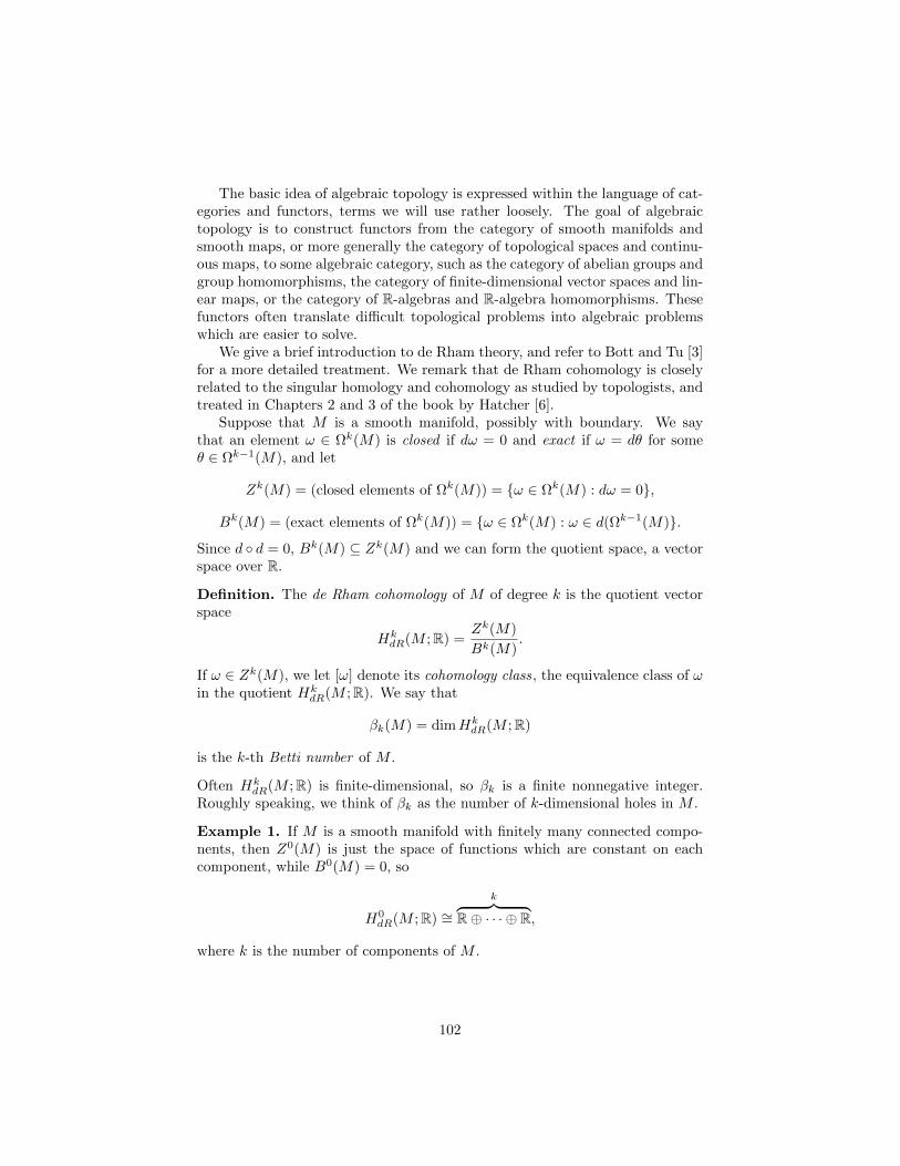
The basic idea of algebraic topology is expressed within the language of cat-egories and functors, terms we will use rather loosely. The goal of algebraictopology is to construct functors from the category of smooth manifolds andsmooth maps, or more generally the category of topological spaces and continu-ous maps, to some algebraic category, such as the category of abelian groups andgroup homomorphisms, the category of finite-dimensional vector spaces and lin-ear maps, or the category of R-algebras and R-algebra homomorphisms. Thesefunctors often translate difficult topological problems into algebraic problemswhich are easier to solve.

We give a brief introduction to de Rham theory, and refer to Bott and Tu [3]for a more detailed treatment. We remark that de Rham cohomology is closelyrelated to the singular homology and cohomology as studied by topologists, andtreated in Chapters 2 and 3 of the book by Hatcher [6].

Suppose that M is a smooth manifold, possibly with boundary. We saythat an element ω ∈ Ωk(M) is closed if dω = 0 and exact if ω = dθ for someθ ∈ Ωk−1(M), and let

Zk(M) = (closed elements of Ωk(M)) = ω ∈ Ωk(M) : dω = 0,

Bk(M) = (exact elements of Ωk(M)) = ω ∈ Ωk(M) : ω ∈ d(Ωk−1(M).

Since d d = 0, Bk(M) ⊆ Zk(M) and we can form the quotient space, a vectorspace over R.

Definition. The de Rham cohomology of M of degree k is the quotient vectorspace

HkdR(M ;R) =

Zk(M)

Bk(M).

If ω ∈ Zk(M), we let [ω] denote its cohomology class, the equivalence class of ωin the quotient Hk

dR(M ;R). We say that

βk(M) = dimHkdR(M ;R)

is the k-th Betti number of M .

Often HkdR(M ;R) is finite-dimensional, so βk is a finite nonnegative integer.

Roughly speaking, we think of βk as the number of k-dimensional holes in M .

Example 1. If M is a smooth manifold with finitely many connected compo-nents, then Z0(M) is just the space of functions which are constant on eachcomponent, while B0(M) = 0, so

H0dR(M ;R) ∼=

k︷ ︸︸ ︷R⊕ · · · ⊕ R,

where k is the number of components of M .

102

Example 2. The reader may recall the method of exact differentials for solvingdifferential equations. This method states that if

ω = Mdx+Ndy ∈ Ω1(R2) satisfies the integrability condition∂N

∂x− ∂M

∂y= 0,

then ω = df for some smooth real-valued function f on R2. In that case,

f = c is a solution to the DE Mdx+Ndy = 0.

The integrability condition is simply the statement that dω = 0 so ω is closed,and the fact that this implies that ω is exact is simply the assertion thatH1dR(R2;R) = 0, a special case of the Poincare Lemma to be presented in the

next section.Suppose on the other hand, that M = R2 − (0, 0) and

ω =xdy − ydxx2 + y2

∈ Ω1(M).

Note that the denominator in this expression is nonzero at all points of M ,since M excludes the point (0, 0, 0) where the expression defining ω blows up.A straightforward calculation shows that ω is closed, but if we let S1 be theunit circle x2 + y2 = 1 with counterclockwise parametrization, we find usingtechniques of vector calculus that∫

S1

ι∗ω = 2π.

where ι : S1 ⊆ R2 is the inclusion. Let us recall how the calculations go: if wedefine a parametrization ι : [0, 2π]→ R2 of S1 ⊆ R2 by

(x ι)(t) = cos t, (y ι)(t) = sin t.

Then

ι∗dx = − sin tdt, ι∗dy = cos tdt, ι∗ω = ι∗(xdy − ydxx2 + y2

)= dt.

Thus ∫S1

ι∗ω =

∫ 2π

0

dt = 2π

as claimed. (Of course, t is really only a well-behaved coordinate on S1 minus apoint, but since ω is smooth and bounded, it suffices for calculating the integral.)It follows from Stokes’ Theorem that ω cannot be exact, and H1

dR(M ;R) isnonzero. The upshot is that the one-dimensional de Rham cohomology detectsthe hole that is missing at the origin.

Example 3. Recall that any smooth manifold M has an imbedding F : M →RN for some N by the Whitney imbedding theorem, and we can use the Eu-clidean metric on RN to construct a Riemannian metric on M . Let (M, 〈·, ·〉)

103

be an n-dimensional oriented Riemannian manifold (constructed in this or someother way), (x1, . . . , xn) a positively oriented coordinate system defined on anopen subset U of M . If

〈·, ·〉 =

n∑i,j=1

gijdxi ⊗ dxj and g = det(gij),

we use the Riemannian metric to define the volume form on U

ΩU =√gdx1 ∧ · · · dxn.

If (x1, . . . , xn) a second positively oriented coordinate system defined on an opensubset U of M ,

〈·, ·〉 =

n∑i,j=1

gijdxi ⊗ dxj =

n∑k,`=1

gk`dxk ⊗ dx` on U ∩ U .

It follows that

gij =

n∑k,`=1

gk`∂xk

∂xi∂x`

∂xj,

so

det(gij) = det(gk`)

[det

(∂xk

∂xi

)]2

or g = g det

(∂xk

∂xi

),

and the volume forms for two different positively oriented coordinate systemsagree on overlaps,

ΩU =√gdx1 ∧ · · · dxn =

√gdx1 ∧ · · · dxn = ΩU on U ∩ U .

Thus the locally defined volume forms fit together to yield a global volume formΩM ∈ Ωn(M). If M is compact and has empty boundary, we could define itsRiemannian geometry volume by the formula

Volume of M =

∫M

ΩM .

The volume form ΩM has degree n, so it must be closed, while its integral isnonzero, so it cannot be exact by Stokes’s Theorem. Hence if M is a compactoriented manifold, Hn

dR(M ;R) 6= 0.

We have seen that if M is a smooth manifold, the exterior derivative yields asequence of vector spaces and linear maps

d−−−−→ Ωk(M)d−−−−→ Ωk+1(M)

d−−−−→ Ωk+2(M)d−−−−→ ,

the linear maps satisfying the identity d d = 0. This is called the de Rhamcochain complex , and is denoted by Ω∗(M). A smooth map F : M → N induces

104

a commutative ladder

d−−−−→ Ωk(N)d−−−−→ Ωk+1(N)

d−−−−→ Ωk+2(N)d−−−−→

F∗

y F∗

y F∗

yd−−−−→ Ωk(M)

d−−−−→ Ωk+1(M)d−−−−→ Ωk+2(M)

d−−−−→

(4.13)

which can be regarded as a homomorphism of cochain complexes, and denotedby F ∗ : Ω∗(N)→ Ω∗(M). It follows from the commutativity of (4.13) that thesmooth map F induces a vector space homomorphism

F ∗ : HkdR(N ;R)→ Hk

dR(M ;R), for each k.

The direct sum

H∗dR(M ;R) =

∞∑k=0

HkdR(M ;R)

is not only a graded vector space, but can be made into what is called a gradedanticommutative algebra over R, the product being the so-called cup product ,which is defined as follows: If

x ∈ HkdR(M ;R) and y ∈ H l

dR(M ;R),

we can write x = [ω] and y = [φ] where ω and φ are closed forms. It followsfrom the formula

d(ω ∧ φ) = dω ∧ φ+ (−1)kω ∧ dφ (4.14)

that the product of closed forms is closed, so ω ∧ φ represents an element ofHm+ldR (M ;R), and we set

x ∪ y = [ω] ∪ [φ] = [ω ∧ φ] ∈ Hk+ldR (M ;R).

Of course, we need to check that the cup product is independent of the choiceof representatives. We leave this as an exercise for the enterprising reader, withthe hint that one uses the following consequence of (4.14):

Bk(M) ∪ Zl(M) ⊆ Bk+l(M), Zk(M) ∪Bl(M) ⊆ Bk+l(M).

Finally, if F : M → N is a smooth map, the fact that

F ∗(ω ∧ φ) = F ∗(ω) ∧ F ∗(φ) ∈ Hm+ldR (M ;R)

implies that the linear map on cohomology

F ∗ : H∗dR(N ;R) −→ H∗dR(M ;R) respects the cup product:

F ∗([ω] ∪ [φ]) = F ∗[ω] ∪ F ∗[φ].

The correspondences

M 7→ H∗dR(M ;R), (F : M → N) 7→ (F ∗ : H∗dR(N ;R)→ H∗dR(M ;R)),

with F ∗ going the opposite direction to F , satisfy the following two axioms:

105

1. The identity map on a given manifold M induces the identity on its deRham cohomology.

2. If F : M → N and G : N → P are smooth maps, then (GF )∗ = F ∗ G∗.

These two identities characterize what is called a contravariant functor from thecategory of smooth manifolds and smooth maps to the category of graded anti-commutative R-algebras and graded R-algebra homomorphisms, contravariantbecause F ∗ goes the opposite direction to F .

Exercise VIII. (Due Friday, December 12.) Suppose that M = R3 −0 withthe standard coordinates (x, y, z), and define ω ∈ Ω2(M) by

ω =xdy ∧ dz + ydz ∧ dx+ zdx ∧ dy

(x2 + y2 + z2)(3/2).

Show that ω is closed but not exact. Explain how this shows that H2(M ;R) 6= 0.Hint: Use spherical coordinates in R3 and integrate over the unit two-spherejust like you would in vector calculus.

Exercise VIIIA. (Do not hand in.) Suppose that X is a smooth vector fieldon M . Define the interior product ιX : Ωk(M)→ Ωk−1(M) by

ιX(ω)(Y1, . . . , Yk−1) = ω(X,Y1, . . . , Yk−1).

Show that if ω ∈ Ωk(M) and θ ∈ Ωl(M), then

ιX(ω ∧ θ) = (ιXω) ∧ θ + (−1)kω ∧ (ιXθ).

4.7 The Poincare Lemma

In order for de Rham cohomology to be useful in solving topological problems,we need to be able to compute it in important cases. There are two main stepsto developing a method for calculating de Rham cohomology. The first consistsof establishing the so-called Poincare Lemma, which calculates the de Rhamcohomology of a convex open subset of Rn. The second is the Mayer-Vietorissequence which provides a technique for computing the homology of M by meansof a cover Uα : α ∈ A of M by open sets each diffeomorphic to a convex opensubset of Rn.

Poincare Lemma. If U is a convex open subset of Rn, then the de Rhamcohomology of U is “trivial”:

HkdR(U ;R) ∼=

R if k = 0,

0 if k 6= 0.

This is a powerful generalization of the method of exact differentials from cal-culus.

106

Instead of proving the Poincare Lemma directly, it is convenient to regardit as a corollary of a more powerful fact about de Rham cohomology: de Rhamcohomology is invariant under smooth homotopy.

We say that smooth maps F,G : M → N are smoothly homotopic if there isa smooth map H : [0, 1]×M → N such that

H(0, p) = F (p) and H(1, p) = G(p).

Homotopy Theorem. Smoothly homotopic maps F,G : M → N betweensmooth manifolds without boundary induce the same map on cohomology,

F ∗ = G∗ : HkdR(N ;R) −→ Hk

dR(M ;R).

To see how the Homotopy Theorem implies the Poincare Lemma, we first notethat if p0 is a single point, regarded as a zero-dimensional manifold, then

Ωk(p0) ∼=

R if k = 0,

0 if k 6= 0.

and hence d ≡ 0 and

HkdR(p0;R) ∼=

R if k = 0,

0 if k 6= 0.

Next observe that if p0 lies within U , then we have an inclusion map ι : p0 → Uand a map r : U → p0 such that r ι = idp0. On the other hand, ι r ishomotopic to the identity on U , because the map H : [0, 1]×U → U defined by

H(t, p) = tp0 + (1− t)p satisfies H(0, p) = p, H(1, p) = p0.

Thus functoriality implies that

ι∗ : H∗dR(U ;R)→ H∗dR(p0;R) and r∗ : H∗dR(p0;R)→ H∗dR(U ;R)

are both isomorphisms.

Proof of Homotopy Theorem: The Homotopy Theorem follows from the specialcase for the homotopic inclusion maps

ι0, ι1 : M −→ [0, 1]×M, ι0(p) = (0, p), ι1(p) = (1, p).

Indeed, if H : [0, 1] ×M → N is a smooth homotopy from F to G, then bydefinition of homotopy, F = H ι0 and G = H ι1, so

ι∗0 = ι∗1 ⇒ F ∗ = ι∗0 H∗ = ι∗1 H∗ = G∗,

proving the Homotopy Theorem.

107

This special case, however, can be established by integration over the fiberof the projection on the second factor [0, 1]×M →M :

Fiber Integration Lemma. For each nonnegative integer k, there is a linearmap

π∗ : Ωk([0, 1]×M)→ Ωk−1(M)

such thatι∗1ω − ι∗0ω = d(π∗(ω)) + π∗(dω). (4.15)

Proof that the Fiber Integration Lemma implies the Homotopy Lemma: Itfollows from (4.15) that if dω = 0,

ι∗1ω − ι∗0ω = d(π∗(ω))⇒ [i∗1ω] = [i∗0ω],

and hence on the cohomology level ι∗0 = ι∗1.

Proof of the Fiber Integration Lemma. Let t be the standard coordinate on [0, 1],T the vector field tangent to the [0, 1] factor in [0, 1]×M such that dt(T ) = 1.We then define integration over the fiber

π∗ : Ωk([0, 1]×M)→ Ωk−1(M) by π∗(ω)(p) =

∫ 1

0

(ιTω)(t, p)dt,

where the interior product (ιTω)(t, p) is the element of ΛkT ∗(t,p)([0, 1]×M) givenby the formula

(ιTω)(t, p)(v1, . . . , vk−1) = ω(t, p)(T (t, p), v1, . . . vk−1),

for v1, . . . , vk−1 ∈ T(t,p)([0, 1]×M).

The integration is possible because the exterior power at (t, p) is canonicallyisomorphic to ΛkT ∗(0,p)([0, 1]×M).

Thus to finish the proof of the Fiber Integration Lemma, it remains only toestablish (4.15). Let (Uα, φα) : α ∈ A be an atlas for M , and let ψα : α ∈ Abe a partition of unity subordinate to Uα : α ∈ A. Since (4.15) is linearas a function of ω it suffices to establish (4.15) for the differential forms ψαωwhich have compact support within Uα. Thus let (U, (x1, . . . , xn) be one of theelements of the atlas, take (t, x1, . . . , xn) as the corresponding smooth coordinatesystem on [0, 1]×U , and suppose that the k-form ω has compact support within[0, 1]× U . Then the above formula for π∗ gives

ω = f(t, x)dxi1 ∧ · · · ∧ dxik ⇒ π∗(ω) = 0, (4.16)

ω = f(t, x)dt ∧ dxi1 ∧ · · · ∧ dxik−1

⇒ π∗(ω) =

[∫ 1

0

f(u, x)du

]dxi1 ∧ · · · ∧ dxik−1 . (4.17)

108

Since any k-form with support in [0, 1] × U is a superposition of differentialforms treated by (4.16) and (4.17), we need only verify the “cochain homotopyformula” (4.15) in each of these two cases.

In the first case (4.16), π∗(ω) = 0 so d(π∗(ω)) = 0. On the other hand,

dω =∂f

∂tdt ∧ dxi1 ∧ · · · ∧ dxik + (terms not involving dt),

so

π∗(dω) =

[∫ 1

0

∂f

∂u(u, x)du

]dxi1 ∧ · · · ∧ dxik

= f(1, x)dxi1 ∧ · · · ∧ dxik − f(0, x)dxi1 ∧ · · · ∧ dxik = ι∗1(ω)− ι∗0(ω),

so the formula is established in this case.In the other case (4.17),

ι∗1(dt) = ι∗0(dt) = 0 ⇒ ι∗1(ω) = ι∗0(ω) = 0. (4.18)

On the one hand,

dω =

n∑j=1

∂f

∂xjdxj ∧ dt ∧ dxi1 ∧ · · · ∧ dxik−1

= −n∑j=1

∂f

∂xjdt ∧ dxj ∧ dxi1 ∧ · · · ∧ dxik−1

and hence

π∗(dω) = −n∑j=1

[∫ 1

0

∂f

∂xj(u, x)du

]dxj ∧ dxi1 ∧ · · · ∧ dxik−1 . (4.19)

On the other hand,

π∗(ω) =

[∫ 1

0

f(u, x)du

]dxi1 ∧ · · · ∧ dxik−1 ,

so

dπ∗(ω) =

n∑j=1

∂

∂xj

[∫ 1

0

f(u, x)du

]dxj ∧ dxi1 ∧ · · · ∧ dxik−1

=

n∑j=1

[∫ 1

0

∂f

∂xj(u, x)du

]dxj ∧ dxi1 ∧ · · · ∧ dxik−1 . (4.20)

In view of (4.18), the desired identity now follows by adding (4.19) and (4.20).

Definition. We say that two smooth manifolds M and N are smoothly homo-topic equivalent if there exist smooth maps F : M → N and G : N → M suchthat G F and F G are both homotopic to the identity.

109

For example, the cylinder is smoothly homotopy equivalent to a circle. Similarly,the punctured plane is smoothly homotopy equivalent to a circle. It followsfrom the Homotopy Theorem that if two manifolds are smoothly homotopyequivalent, they have the same de Rham cohomology.

4.8 Applications of de Rham theory

In this section, we give two applications of de Rham’s cohomology, first an easyproof of the Brouwer fixed point theorem, which states that a continuous mapfrom the unit disk to itself must contain a fixed point, and second a proof thatit is not possible to comb the hair on a billiard ball.

For the Brouwer fixed point theorem, we consider the unit disk

Dn = (x1, . . . , xn) ∈ Rn : (x1)2 + · · ·+ (xn)2 ≤ 1,

a smooth manifold with boundary, the boundary being

Sn−1 = (x1, . . . , xn) ∈ Rn : (x1)2 + · · ·+ (xn)2 = 1.

Lemma 4.8.1. If n ≥ 2, there does not exist a smooth map F : Dn → Sn−1

which leaves Sn−1 pointwise fixed.

Proof: Suppose that there were such a map F , and let p0 = F (0). Define

H : [0, 1]× Sn−1 → Sn−1 by H(t, p) = F (tp).

Then H is a smooth homotopy from c to id where c is the constant map whichtakes Sn−1 to p0 and id is the identity map of Sn−1. By the Homotopy Theorem,

c∗ = id∗ : Hn−1dR (Sn−1;R)→ Hn−1

dR (Sn−1;R).

If ω is a smooth (n − 1)-form on Sn−1, c∗(ω) = 0 since c is constant, andhence c∗ is the zero map on Hn−1

dR (Sn−1;R). On the other hand, it follows fromStokes’s Theorem that Hn−1

dR (Sn−1;R) 6= 0, so id∗ = id is not the zero map, acontradiction.

Proposition 4.8.2. A smooth map G : Dn → Dn must have a fixed point.

Proof: If G : Dn → Dn is a smooth map with no fixed point, define F : Dn →Sn−1 as follows: For p ∈ Dn, let L(p) denote the line through p and G(p) andlet F (p) be the point on Sn−1 ∩L(p) closer to p than G(p). Since G is smooth,F is also smooth. Moreover, F leaves Sn−1 pointwise fixed, contradicting theprevious lemma.

Theorem 4.8.3 (Brouwer Fixed Point Theorem). A continuous mapf : Dn → Dn must have a fixed point.

110

Proof: Suppose that f : Dn → Dn is a continuous map and ε > 0 is given.By the Weierstrass approximation theorem, there is a smooth polynomial mapP : Dn → Rn such that |P (p)− f(p)| < ε for p ∈ Dn. let

G =1

1 + εP.

Then G : Dn → Dn is a smooth map which approximates f arbitrarily closely.Suppose now that f : Dn → Dn is a continuous map without fixed points

and letµ = inf|f(p)− p| : p ∈ Dn.

By the argument in the preceding paragraph, we can choose a smooth mapG : Dn → Dn such that |f − G| < µ. Then G is a smooth map without fixedpoints, contradicting the preceding proposition.

Remark. The proof of Theorem 4.8.3 illustrates that it is sometimes possibleto obtain topological results involving continuous maps by approximation fromthe theory of smooth manifolds and smooth maps.

We next prove that there is no smooth nowhere zero vector field tangent to S2.This makes use of the cohomology of SO(3) which we will show how to computein the next section. The result is that

HkdR(SO(3);R) = Hk

dR(RP 3;R) ∼=

R, if k = 0 or k = 3,

0, otherwise.(4.21)

Theorem 4.8.4. Any smooth vector field X : S2 → TS2 must have a zero.

Proof: We suppose that S2 has a nowhere vanishing tangent vector field X :S2 → TS2 and derive a contradiction.

Recall that S2 = (x, y, z) ∈ R3 : x2 + y2 + z2 = 1. Define the inclusionmap

E3 : S2 → R3 by E3(x, y, z) = (x, y, z) ∈ R3.

If p ∈ R3, we can regard E3(p) as the outward pointing unit normal to S2.Define

E1 : S2 → R3 by E1(p) =1

|X(p)|X(p).

Finally, use the cross product to define

E2 : S2 → R3 by E2(p) = E3(p)× E1(p).

For each p ∈ S2, we have a positively oriented orthonormal frame

(E1(p), E2(p), E3(p)) for R3.

There is a unique matrix

A(p) =

a11(p) a1

2(p) a13(p)

a21(p) a2

2(p) a23(p)

a31(p) a3

2(p) a33(p)

∈ SO(3)

111

such that

(E1(p) E2(p) E3(p)

)=(i j k

)a11(p) a1

2(p) a13(p)

a21(p) a2

2(p) a23(p)

a31(p) a3

2(p) a33(p)

,

and we have a smooth map A : S2 → SO(3) which takes p to A(p). We alsohave a smooth projection π : SO(3)→ S2, defined by

π

a11(p) a1

2(p) a13(p)

a21(p) a2

2(p) a23(p)

a31(p) a3

2(p) a33(p)

=

a13(p)a2

3(p)a3

3(p)

,

such that π A = id. Thus the identity map factors through the composition

S2 A−−−−→ SO(3)π−−−−→ S2,

and we can apply the contravariant functor H2 to obtain a factorization of theidentity

H2dR(S2;R)

π∗

−−−−→ H2dR(SO(3);R)

A∗

−−−−→ H2dR(S2;R).

SinceH2dR(SO(3);R) = 0 and H2

dR(S2;R) ∼= R,

this yields a contradiction. QED

4.9 The Mayer-Vietoris Sequence*

In order to be able to calculate de Rham cohomology effectively, we need onefurther property of de Rham cohomology, the exactness of the so-called Mayer-Vietoris sequence. In this section, we will describe the Mayer-Vietoris sequenceand show how to use it to calculate the de Rham cohomology of a smoothmanifold by dividing it up into simpler pieces.

A sequence of vector spaces and linear maps,

· · · → Vi−1Ti−1−−−−→ Vi

Ti−−−−→ Vi+1 → · · ·,

extending infinitely far in each direction, is said to be exact if

Im(Ti−1) = Ker(Ti)

for each i. In particular, the sequence

0→ V0T1−−−−→ V1

T2−−−−→ V2 → 0,

is a short exact sequence if

1. T1 is injective,

112

2. T2 is surjective, and

3. Im(T1) = Ker(T2).

Suppose that U and V are open subsets of a smooth manifold M such thatM = U ∪ V . We then have a diagram of inclusion maps:

U ∩ V jU−−−−→ U

jV

y iU

yV

iV−−−−→ M

Using this diagram, we can construct a sequence of vector spaces and linearmaps

0→ Ωk(M)i∗−−−−→ Ωk(U)⊕ Ωk(V )

j∗−−−−→ Ωk(U ∩ V )→ 0, (4.22)

where

i∗(ω) = (i∗U (ω), i∗V (ω)), j∗(φU , φV ) = j∗U (φU )− j∗V (φV ).

Since i∗ and j∗ commute with d, (4.22) yields a sequence of cochain complexes

0→ Ω∗(M)i∗−−−−→ Ω∗(U)⊕ Ω∗(V )

j∗−−−−→ Ω∗(U ∩ V )→ 0. (4.23)

Lemma 4.9.1. The sequence (4.23) is exact; in other words for each k, thesequence (4.22) of vector spaces and linear maps is exact.

One easily checks that i∗ is injective and j∗ i∗ = 0. If j∗(φU , φV ) = 0, thenj∗U (φU ) = j∗V (φV ) so j∗U (φU ) and j∗V (φV ) fit together to form a smooth form onM such that i∗(ω) = (φU , φV ).

The only difficult step in the proof is to show that j∗ is surjective. To dothis, we choose a partition of unity ψU , ψV subordinate to the open coverU, V of M . If θ ∈ Ωk(U ∩ V ), we define φU ∈ Ωk(U) by

φU (p) =

ψV (p)θ(p), for p ∈ U ∩ V ,0, for p ∈ U − (U ∩ V ),

and φV ∈ Ωk(V ) by

φV (p) =

−ψU (p)θ(p), for p ∈ U ∩ V ,0, for p ∈ V − (U ∩ V ).

thenj∗(φU , φV ) = φU |(U ∩ V )− φV |(U ∩ V ) = ψV θ + ψUθ = θ,

so j∗ is surjective and the lemma is proven.

113

The lemma yields a large commutative diagram in which the rows are exact:

d

y d

y d

y0→ Ωk(M)

i∗−−−−→ Ωk(U)⊕ Ωk(V )j∗−−−−→ Ωk(U ∩ V )→ 0

d

y d

y d

y0→ Ωk+1(M)

i∗−−−−→ Ωk+1(U)⊕ Ωk+1(V )j∗−−−−→ Ωk+1(U ∩ V )→ 0

d

y d

y d

y

(4.24)

Note that i∗ and j∗ induce homomorphisms on cohomology

i∗ : HkdR(M ;R)→ Hk

dR(U ;R)⊕HkdR(V ;R),

j∗ : HkdR(U ;R)⊕Hk

dR(V ;R)→ HkdR(U ∩ V ;R). (4.25)

The commuting diagram (4.24) allows us to construct a “connecting homomor-phism”

∆ : HkdR(U ∩ V ;R)→ Hk+1

dR (M ;R) (4.26)

as follows: If [θ] ∈ HkdR(U ∩ V ;R), choose a representative θ ∈ Ωk(U ∩ V ).

Since j∗ is surjectve, we can choose φ ∈ Ωk(U) ⊕ Ωk(V ) so that j∗(φ) = θ.Then j∗(dφ) = dj∗(φ) = dθ = 0, so there is a unique ω ∈ Ωk+1(M) such thati∗ω = dφ. Finally, i∗(dω) = d(i∗ω) = d(dφ) = 0, and since i∗ is injective,dω = 0. Let [ω] be the de Rham cohomology class of ω in Hk+1

dR (M ;R) and set∆([θ]) = [ω]. Roughly speaking

∆ = (i∗)−1 d (j∗)−1.

By the technique of “diagram chasing”, one checks that ∆([θ]) is independentof the choice of φ, or of θ representing [θ].

We can describe ∆ explicitly as follows: If θ is a representative of [θ] ∈HkdR(U ∩ V ;R), then ∆([θ]) is represented by the form

d(ψV θ) = dψV ∧ θ or − d(ψUθ) = −dψU ∧ θ,

two expressions for the same (k + 1)-form on M (since ψU + ψV = 1) whichactually has its support in U ∩ V .

Theorem 4.9.2. (Mayer-Vietoris) The homomorphisms (4.25) and (4.26)fit together to form a long exact sequence

· · · → HkdR(M ;R)→ Hk

dR(U ;R)⊕HkdR(V ;R)→ Hk

dR(U ∩ V ;R)

→ Hk+1dR (M ;R)→ Hk+1

dR (U ;R)⊕Hk+1dR (V ;R)→ · · · . (4.27)

114

This exact sequence is called the Mayer-Vietoris sequence. Together with theHomotopy Lemma, the Mayer-Vietoris sequence is very helpful in computingthe de Rham cohomology.

The proof of exactness of the Mayer-Vietoris sequence follows from the so-called“snake lemma” from algebraic topology: A short exact sequence of cochaincomplexes such as (4.23) gives rise to a long exact sequence in cohomology suchas (4.27).

To prove the snake lemma one must establish three assertions:

1. Ker(j∗) = Im(i∗),

2. Ker(∆) = Im(j∗), and

3. Ker(i∗) = Im(∆).

Each of these assertions is proven by a diagram chase using the diagram (4.24).(These diagram chases are not difficult, but one could argue that they are bestdone in the privacy of one’s own study. Alternatively, some may prefer to followthe proof of the Snake Lemma in the 1980 movie, “It’s My Turn” starring JillClayburgh.)

For example, suppose we want to check the second of these assertions,Ker(∆) = Im(j∗). To see that Im(j∗) ⊆ Ker(∆), we suppose [θ] ∈ Im(j∗),so [θ] = j∗[φ] for some [φ] ∈ Hk⊕Hk(V ). Then there are representatives θ andφ such that j∗φ = θ. Note that dφ = 0. Hence

∆([θ]) = [(i∗)−1 d (j∗)−1(θ)] = 0.

Conversely, suppose that [θ] ∈ Ker(∆), so (i∗)−1 d (j∗)−1(θ) is exact, so ifφ ∈ (j∗)−1(θ), then (i∗)−1 dφ = dω, for some ω ∈ Ωk(M). Then d(φ−i∗ω) = 0and j∗(φ− i∗ω) = θ. Thus [θ] ∈ Im(j∗).

The other two assertions are proven by similar arguments. A completelydetailed proof would follow exactly the same steps as in the proof of Theorem2.16 in Hatcher [6].

Example 1. We first calculate the cohomology of S1 = (x, y) ∈ R2 : x2 +y2 =1, noting that H0(S1) is isomorphic to the space R of constant functions onS1. We decompose S1 into a union of two open sets

U = S1 ∩y > −1

2

, V = S1 ∩

y <

1

2

,

and note that U and V are both diffeomorphic to open intervals, while U ∩V isdiffeomorphic to the union of two open intervals, so the cohomologies of thesespaces can be calculated from the Poincare Lemma. It follows from the Mayer-Vietoris sequence that

0→ H0(S1)→ H0(U)⊕H0(V )→ H0(U ∩ V )

→ H1(S1)→ H1(U)⊕H1(V )→ H1(U ∩ V )→ · · · ,

115

which yields

0→ R→ R⊕ R→ R⊕ R→ H1(S1)→ 0→ 0→ · · · .

It follows that

HkdR(S1;R) ∼=

R, if k = 0 or k = 1,

0, otherwise.

Example 2. We next consider S2 = (x, y, z) ∈ R3 : x2 + y2 + z2 = 1. Onceagain H0(S2) ∼= R. This time we decompose S2 into a union of

U = S2 ∩z > −1

2

and V = S2 ∩

z <

1

2

.

In this case, U and V are both diffeomorphic to open disks, while U ∩ V ishomotopy equivalent to S1. It follows from the Mayer-Vietoris sequence that

0→ H0(S2)→ H0(U)⊕H0(V )→ H0(U ∩ V )

→ H1(S2)→ H1(U)⊕H1(V )→ H1(U ∩ V )

→ H2(S2)→ H2(U)⊕H2(V )→ H2(U ∩ V )→ · · · ,

which yields

0→ R→ R⊕ R→ R→ H1(S2)→ 0→ R→ H2(S2)→ 0→ · · · .

It follows that

HkdR(S2;R) ∼=

R, if k = 0 or k = 2,

0, otherwise.

Example 3. By induction, one can calculate the cohomology of Sn:

HkdR(Sn;R) ∼=

R, if k = 0 or k = n,

0, otherwise.

The following exercises illustrate how one can use the Poincare Lemma andthe Mayer-Vietoris sequence to calculate the de Rham cohomology of manymanifolds. Further examples are given in [3].

Exercise IXA. (Do not hand in.) a. Determine the de Rham cohomology ofR2 minus a point, which is homotopy equivalent to the disk minus a smallerdisk.

b. Use the Mayer-Vietoris sequence to determine the de Rham cohomology ofR2 minus k points, which is homotopy equivalent to the disk minus k smallerdisks, where k ∈ N.

116

c. Use the Mayer-Vietoris sequence to determine

dimHkdR(Σg;R),

where Σg is the two-sphere with g handles, the compact oriented surface ofgenus g. Hint: Use the fact that Σg is orientable and therefore has a volumeform which makes the top cohomology nonzero.

Exercise IXB. (Do not hand in.) a. Use the Mayer-Vietoris sequence todetermine the de Rham cohomology of RP 2.

b. Use the Mayer-Vietoris sequence to determine the de Rham cohomology ofRP 3 = SO(3), thereby establishing (4.21).

4.10 The Hodge star*

In the last few sections, we have described the foundations for algebraic topol-ogy from the viewpoint of differential forms on smooth manifold. Of course,one can regard topology as simply a beautiful edifice in its own right, but italso has numerous applications to the partial differential equations which arisein geometry. This connection between geometry and topology has become in-creasingly important over the past several decades. Our next goal is to describeone application of de Rham theory, Hodge’s theorem, which states that any deRham cohomology class contains a unique solution to Laplace’s equation.

The first step in this theory consists of constructing the Hodge star, whichgeneralizes the cross product from R3 to Riemannian manifolds of arbitrarydimension.

To construct the Hodge star, we begin with an oriented Riemannian manifold(M, 〈, ·, ·〉) of dimension n without boundary. Recall that for each p ∈ M , thenondegenerate symmetric billinear form 〈·, ·〉 defines an isomorphism

[ : TpM → T ∗pM, [(v) = 〈v, ·〉, with inverse ] : T ∗pM → TpM.

These isomorphisms allow us to transport the nondegenerate symmetric bilinearform

〈·, ·〉 : TpM × TpM → R to 〈·, ·〉 : T ∗pM × T ∗pM → R.

If (x1, . . . , xn) is a smooth coordinate system on U ⊆M , and

〈·, ·〉|U =

n∑i,j=1

gijdxi ⊗ dxj ,

then on the cotangent space we have

〈dxi|p, dxj |p〉 = gij(p),

where (gij(p)) is the matrix inverse to gij(p).

117

We can extend 〈·, ·〉 from T ∗pM to the entire exterior algebra Λ∗T ∗pM . First,we define a multilinear map

µ :

k︷ ︸︸ ︷(T ∗pM × · · · × T ∗pM)×

k︷ ︸︸ ︷(T ∗pM × · · · × T ∗pM)→ R

by

µ((α1, . . . , αk), (β1, . . . , βk)) = det

〈α1, β1〉 · · · 〈α1, βk〉· ·

〈αk, β1〉 · · · 〈αk, βk〉

.

This map is skew-symmetric in each set of k variables, when the other is keptfixed, so it defines a symmetric bilinear form

〈·, ·〉 : ΛkT ∗pM × ΛkT ∗pM → R

such that

〈α1 ∧ · · · ∧ αk, β1 ∧ · · · ∧ βk〉 = det

〈α1, β1〉 · · · 〈α1, βk〉· ·

〈αk, β1〉 · · · 〈αk, βk〉

. (4.28)

and one can check that this symmetric bilinear form 〈·, ·〉 is positive definite onΛkT ∗pM . One sees this most easily by noting that if (θ1, . . . , θn) is an orthonor-mal basis for T ∗pM , then

θi1 ∧ · · · ∧ θik : i1 < · · · < ik

is an orthonormal basis for ΛkT ∗pM . Hence⟨∑ai1···ikθ

i1 ∧ · · · ∧ θik ,∑

ai1···ikθi1 ∧ · · · ∧ θik

⟩=∑

(ai1···ik)2 ≥ 0,

with equality if and only if all the ai1···ik ’s are zero.Recall that if (x1, . . . , xn) is a positively oriented coordinate system on U ⊆

M , the volume form on U is

Ω|U =√|det(gij)|dx1 ∧ · · · ∧ dxn,

and the Ω|U ’s fit together to yield a globally defined volume form Ω on M . If(θ1, . . . , θn) is a basis of smooth one-forms on U such that 〈θi, θj〉 = δij , wesay it is an orthonormal coframe on U . Then Ω|U = ±θ1 ∧ · · · ∧ θn and whenthe plus sign occurs we say that (θ1, . . . , θn) is positively oriented . Using thevolume form, we will now define a linear map

? : ΛkT ∗pM −→ Λn−kT ∗pM

to be called the Hodge star .

118

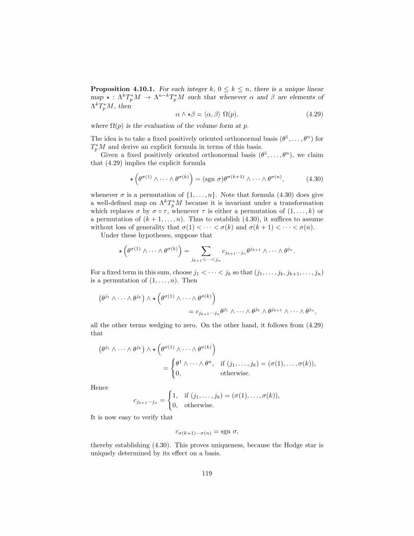
Proposition 4.10.1. For each integer k, 0 ≤ k ≤ n, there is a unique linearmap ? : ΛkT ∗pM → Λn−kT ∗pM such that whenever α and β are elements of

ΛkT ∗pM , thenα ∧ ?β = 〈α, β〉 Ω(p), (4.29)

where Ω(p) is the evaluation of the volume form at p.

The idea is to take a fixed positively oriented orthonormal basis (θ1, . . . , θn) forT ∗pM and derive an explicit formula in terms of this basis.

Given a fixed positively oriented orthonormal basis (θ1, . . . , θn), we claimthat (4.29) implies the explicit formula

?(θσ(1) ∧ · · · ∧ θσ(k)

)= (sgn σ)θσ(k+1) ∧ · · · ∧ θσ(n), (4.30)

whenever σ is a permutation of 1, . . . , n. Note that formula (4.30) does givea well-defined map on ΛkT ∗pM because it is invariant under a transformationwhich replaces σ by σ τ , whenever τ is either a permutation of (1, . . . , k) ora permutation of (k + 1, . . . , n). Thus to establish (4.30), it suffices to assumewithout loss of generality that σ(1) < · · · < σ(k) and σ(k + 1) < · · · < σ(n).

Under these hypotheses, suppose that

?(θσ(1) ∧ · · · ∧ θσ(k)

)=

∑jk+1<···<jn

cjk+1···jnθjk+1 ∧ · · · ∧ θjn .

For a fixed term in this sum, choose j1 < · · · < jk so that (j1, . . . , jk, jk+1, . . . , jn)is a permutation of (1, . . . , n). Then(

θj1 ∧ · · · ∧ θjk)∧ ?(θσ(1) ∧ · · · ∧ θσ(k)

)= cjk+1···jnθ

j1 ∧ · · · ∧ θjk ∧ θjk+1 ∧ · · · ∧ θjn ,

all the other terms wedging to zero. On the other hand, it follows from (4.29)that(

θj1 ∧ · · · ∧ θjk)∧ ?(θσ(1) ∧ · · · ∧ θσ(k)

)=

θ1 ∧ · · · ∧ θn, if (j1, . . . , jk) = (σ(1), . . . , σ(k)),

0, otherwise.

Hence

cjk+1···jn =

1, if (j1, . . . , jk) = (σ(1), . . . , σ(k)),

0, otherwise.

It is now easy to verify that

cσ(k+1)···σ(n) = sgn σ,

thereby establishing (4.30). This proves uniqueness, because the Hodge star isuniquely determined by its effect on a basis.

119

To prove existence, one uses (4.30) to define the Hodge star on a fixedorthonormal basis, and checks that it satisfies (4.29). This is an easy verificationwhich we leave to the diligent reader.

Note that it follows from the proof that if (θ1, . . . , θn) is any positivelyoriented orthonormal basis for T ∗pM , then (4.30) holds for that basis. This factis extremely useful in calculating the Hodge star.

Remark: One can give a very useful geometric interpretation of the Hodge star.Suppose that W is a k-dimensional subspace of T ∗pM with orthonormal basis

(θ1, . . . , θk). Complete (θ1, . . . , θk) to a positively oriented orthonormal basis(θ1, . . . , θn) for T ∗pM . Then (θk+1, . . . , θn) is a positively oriented orthonormal

basis for the oriented orthogonal complement W⊥ to W in T ∗pM .

Of course, the Hodge star extends immediately to a linear map

? : Ωk(M)→ Ωn−k(M)

which is also called the Hodge star. It is easy to verify that

?(?α) = (−1)k(n−k)α, for α ∈ Ωk(M). (4.31)

Example 1. We first consider R2 with its usual Euclidean inner product andthe Euclidean coordinates (x, y). In this case, Θ = ?1 = dx ∧ dy, and

?(dx) = dy, ?(dy) = −dx, so ? (Pdx+Qdy) = −Qdx+ Pdy.

We can think of the Hodge star on R2 as a counterclockwise rotation through90 degrees. More generally, if (M, 〈, ·, ·〉) is an oriented two-dimensional Rie-mannian manifold, we can define a counterclockwise rotation through 90 degrees

J : Ω1(M)→ Ω1(M) by J(ω) = ?(ω).

Example 2. We next consider R3 with its usual Euclidean inner productand the Euclidean coordinates (x, y, z). In this case, Θ = ?1 = dx ∧ dy ∧ dz.Moreover,

?(dx) = dy ∧ dz, ?(dy) = dz ∧ dx, ?(dz) = dx ∧ dy,

?(dy ∧ dz) = dx, ?(dz ∧ dx) = dy, ?(dx ∧ dy) = dz.

Note that if α and β are elements of Ω1(E3), then so is ?(α ∧ β), and one cancheck that its components are the same as those of the cross product α×β. Moregenerally, if (M, 〈, ·, ·〉) is an oriented three-dimensional Riemannian manifoldwe can define a cross product

× : Ω1(M)× Ω1(M)→ Ω1(M) by α× β = ?(α ∧ β).

120

4.11 Lorentz manifolds; Maxwell’s equations*

(Note: This section provides an application to physics which can be skippedwithout loss of continuity.) The notion of Riemannian manifold has a general-ization which is extremely useful in Einstein’s theory of general relativity [14]and the Hodge star can be extended to this context. This provides a simplifi-cation of the equations of electricity and magnetism and gives them a de Rhamcohomology interpretation—one of the reasons that de Rham cohomology isimportant to physics.

Definition. Let M be a smooth manifold. A pseudo-Riemannian metric on Mis a function which assigns to each p ∈ M a nondegenerate symmetric bilinearmap

〈·, ·〉p : TpM × TpM −→ R

which which varies smoothly with p ∈M . (Positive definite implies nondegener-ate, so any Riemannian metric is also a pseudo-Riemannian metric.) As before,varying smoothly with p ∈ M means that if φ = (x1, . . . , xn) : U → Rn is asmooth coordinate system on M , then for p ∈ U ,

〈·, ·〉p =

n∑i,j=1

gij(p)dxi|p ⊗ dxj |p,

where the functions gij : U → R are smooth. The conditions that 〈·, ·〉p besymmetric and nondegenerate are expressed by saying that (gij) is a symmetricmatrix and has nonzero determinant.

It follows from linear algebra that for any choice of p ∈M , local coordinates(x1, . . . , xn) can be chosen so that

(gij(p)) =

(−Ip×p 0

0 Iq×q

),

where Ip×p and Iq×ql are p × p and q × q identity matrices with p + q = n.The pair (p, q) is called the signature of the pseudo-Riemannian metric. Apseudo-Riemannian metric of signature (0, n) is just a Riemannian metric. Apseudo-Riemannian metric of signature (1, n− 1) is called a Lorentz metric.

A pseudo-Riemannian manifold is a pair (M, 〈·, ·〉) where M is a smoothmanifold and 〈·, ·〉 is a pseudo-Riemannian metric on M . Similarly, a Lorentzmanifold is a pair (M, 〈·, ·〉) where M is a smooth manifold and 〈·, ·〉 is a Lorentzmetric on M .

Example. Let Rn+1 be given coordinates (t, x1, . . . , xn), with t being regardedas time and (x1, . . . , xn) being regarded as Euclidean coordinates in space, andconsider the Lorentz metric

〈·, ·〉 = −c2dt⊗ dt+

n∑i=1

dxi ⊗ dxi,

121

where the constant c is regarded as the speed of light. When endowed with thismetric, Rn+1 is called Minkowski space-time and is denoted by Ln+1. Four-dimensional Minkowski space-time is the arena for special relativity .

The arena for general relativity is a more general four-dimensional Lorentz man-ifold (M, 〈·, ·〉), also called space-time. In the case of general relativity, thecomponents gij of the metric are regarded as potentials for the gravitationalforces.

In either case, points of space-time can be thought of as events that happenat a given place in space and at a given time. The trajectory of a moving particlecan be regarded as curve of events, called its world line.

If p is an event in a Lorentz manifold (M, 〈·, ·〉), the tangent space TpMinherits a Lorentz inner product

〈·, ·〉p : TpM × TpM −→ R.

We say that an element v ∈ TpM is

1. timelike if 〈v, v〉 < 0,

2. spacelike if 〈v, v〉 > 0, and

3. lightlike if 〈v, v〉 = 0.

A parametrized curve γ : [a, b] → M into a Lorentz manifold (M, 〈·, ·〉) is saidto be timelike if γ′(u) is timelike for all u ∈ [a, b]. If a parametrized curveγ : [a, b] → M represents the world line of a massive object, it is timelike andthe integral

L(γ) =1

c

∫ b

a

√−〈γ′(u)γ′(u)〉du (4.32)

is the elapsed time measured by a clock moving along the world line γ. We callL(γ) the elapsed proper time along γ.

The Twin Paradox. The fact that elapsed time is measured by the integral(4.32) has counterintuitive consequences. Suppose that γ : [a, b] → L4 is atimelike curve in four-dimensional Minkowski space-time, parametrized so that

γ(t) = (t, x1(t), x2(t), x3(t)).

Then

γ′(t) =∂

∂t+

3∑i=1

dxi

dt

∂

∂xi, so 〈γ′(t), γ′(t)〉 = −c2 +

3∑i=1

(dxi

dt

)2

,

and hence

L(γ) =

∫ b

a

1

c

√√√√c2 −3∑i=1

(dxi

dt

)2

dt =

∫ b

a

√√√√1− 1

c2

3∑i=1

(dxi

dt

)2

dt. (4.33)

122

Thus if a clock is at rest with respect to the coordinates, that is dxi/dt ≡ 0,it will measure the time interval b − a, while if it is in motion it will measurea somewhat shorter time interval. This failure of clocks to synchronize is whatis called the twin paradox. An example of this is provided by the differentialaging of characters in the recent Hollywood film, “Interstellar.”

The Hodge star can be extended to arbitrary pseudo-Riemannian manifolds. Todo this one first defines a nondegenerate symmetric bilinear form

〈·, ·〉 : ΛkT ∗pM × ΛkT ∗pM → R

by (4.28) and says that a basis (θ1, . . . , θn) for T ∗pM is orthonormal if

(〈θi, θj〉) =

(−Ip×p 0

0 Iq×q

),

where p+ q = n. There are two possible signs for the volume form

Ω|U = ±θ1 ∧ · · · ∧ θn.

This sign depends upon convention which might differ from author to author.Once the sign is chosen one defines the Hodge star ? : ΛkT ∗pM → Λn−kT ∗pM by

α ∧ ?β = 〈α, β〉 Ω(p),

just as in the Riemannian case.

Example. Let us consider the Hodge star in Minkowski space-tme L4 with itsstandard coordinates (t, x, y, z), taking the speed of light to be c = 1 so thatthe Lorentz metric is

〈·, ·〉 = −dt⊗ dt+ dx⊗ dx+ dy ⊗ dy + dz ⊗ dz. (4.34)

In this case, the volume form is

Ω = ?1 = dt ∧ dx ∧ dy ∧ dz.

Clearly, ?(dt ∧ dx) = ±dy ∧ dz. To determine the sign, we note that

〈dt ∧ dx, dt ∧ dx〉 = −1, so (dt ∧ dx)(?dt ∧ dx) = −Ω.

It follows that

?(dt ∧ dx) = −dy ∧ dz, ?(dt ∧ dy) = −dz ∧ dy, ?(dt ∧ dz) = −dx ∧ dy.

By similar arguments, one verifies that

?(dy ∧ dz) = dt ∧ dx, ?(dz ∧ dx) = dt ∧ dy, ?(dx ∧ dy) = dt ∧ dz.

This Hodge star is invariant under orientation-preserving Lorentz transforma-tion, those orientation-preserving linear transformations of L4 which leave in-variant the flat Lorentz metric (4.34).

123

Maxwell’s equations. Using the Hodge star on Minkowski space-time withthe standard Lorentz metric, we can give a particularly elegant formulationof Maxwell’s equations from electricity and magnetism, equations formulatedby James Clerk Maxwell in 1873. This formulation has the advantage that itextends to the curved space-times of general relativity.

In Maxwell’s theory of electricity and magnetism, one imagines that one isgiven the charge density ρ(t, x, y, z) and the current density

J(t, x, y, z) = Jx∂

∂x+ Jy

∂

∂y+ Jz

∂

∂z.

The charge and current density should determine the electric and magnetic fields

E(t, x, y, z) = Ex∂

∂x+ Ey

∂

∂y+ Ez

∂

∂z= (electric field)

and B(t, x, y, z) = Bx∂

∂x+By

∂

∂y+Bz

∂

∂z= (magnetic field)

by means of Maxwell’s equations, which are expressed in terms of the divergenceand curl operations studied in second year calculus as

∇ ·B = 0, ∇×E +∂B

∂t= 0, (4.35)

∇ ·E = 4πρ, ∇×B− ∂E

∂t= 4πJ. (4.36)

To express these equations in space-time formalism, it is convenient to re-place the electric and magnetic fields by a single covariant tensor field of ranktwo, the so called Faraday tensor :

F = −Exdt ∧ dx− Eydt ∧ dy − Ezdt ∧ dz+Bxdy ∧ dz +Bydz ∧ dx+Bzdx ∧ dy.

Then the Hodge star interchanges the E and the B fields:

? F = Bxdt ∧ dx+Bydt ∧ dy +Bzdt ∧ dz+ Exdy ∧ dz + Eydz ∧ dx+ Ezdx ∧ dy.

Exercise XA. (Do not hand in.) a. Show that in Minkowski space-time L4,

?? = (−1)k+1 : Ωk(L4) −→ Ωk(L4).

b. Determine ?dt, ?dx, ?dy and ?dz.

c. Show that Maxwell’s equations can be expressed in terms of the Faradaytensor as

dF = 0, d(?F) = ?(4πJ ),

where J = −ρdt+ Jxdx+ Jydy + Jzdz. (4.37)

124

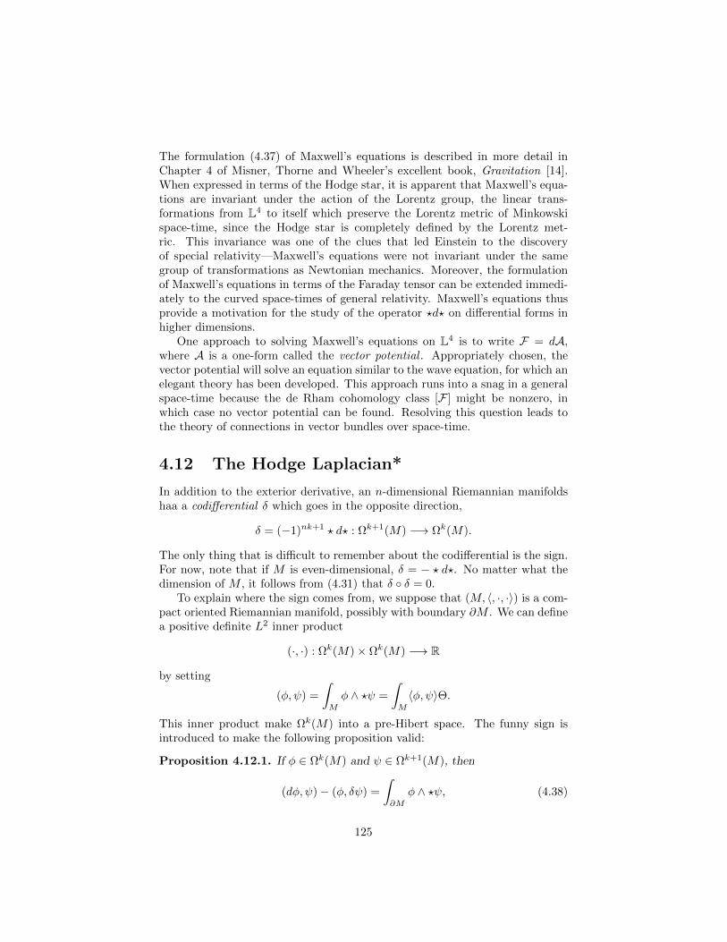
The formulation (4.37) of Maxwell’s equations is described in more detail inChapter 4 of Misner, Thorne and Wheeler’s excellent book, Gravitation [14].When expressed in terms of the Hodge star, it is apparent that Maxwell’s equa-tions are invariant under the action of the Lorentz group, the linear trans-formations from L4 to itself which preserve the Lorentz metric of Minkowskispace-time, since the Hodge star is completely defined by the Lorentz met-ric. This invariance was one of the clues that led Einstein to the discoveryof special relativity—Maxwell’s equations were not invariant under the samegroup of transformations as Newtonian mechanics. Moreover, the formulationof Maxwell’s equations in terms of the Faraday tensor can be extended immedi-ately to the curved space-times of general relativity. Maxwell’s equations thusprovide a motivation for the study of the operator ?d? on differential forms inhigher dimensions.

One approach to solving Maxwell’s equations on L4 is to write F = dA,where A is a one-form called the vector potential . Appropriately chosen, thevector potential will solve an equation similar to the wave equation, for which anelegant theory has been developed. This approach runs into a snag in a generalspace-time because the de Rham cohomology class [F ] might be nonzero, inwhich case no vector potential can be found. Resolving this question leads tothe theory of connections in vector bundles over space-time.

4.12 The Hodge Laplacian*

In addition to the exterior derivative, an n-dimensional Riemannian manifoldshaa a codifferential δ which goes in the opposite direction,

δ = (−1)nk+1 ? d? : Ωk+1(M) −→ Ωk(M).

The only thing that is difficult to remember about the codifferential is the sign.For now, note that if M is even-dimensional, δ = − ? d?. No matter what thedimension of M , it follows from (4.31) that δ δ = 0.

To explain where the sign comes from, we suppose that (M, 〈, ·, ·〉) is a com-pact oriented Riemannian manifold, possibly with boundary ∂M . We can definea positive definite L2 inner product

(·, ·) : Ωk(M)× Ωk(M) −→ R

by setting

(φ, ψ) =

∫M

φ ∧ ?ψ =

∫M

〈φ, ψ〉Θ.

This inner product make Ωk(M) into a pre-Hibert space. The funny sign isintroduced to make the following proposition valid:

Proposition 4.12.1. If φ ∈ Ωk(M) and ψ ∈ Ωk+1(M), then

(dφ, ψ)− (φ, δψ) =

∫∂M

φ ∧ ?ψ, (4.38)

125

where δ = (−1)nk+1 ? d?.

The proposition is a consequence of Stokes’ Theorem:∫∂M

φ ∧ ?ψ =

∫M

d(φ ∧ ?ψ) =

∫M

dφ ∧ ?ψ + (−1)k∫M

φ ∧ (d ? ψ)

=

∫M

dφ ∧ ?ψ + (−1)k(−1)(n−k)k

∫M

φ ∧ ?(?d ? ψ)

=

∫M

dφ ∧ ?ψ −∫M

φ ∧ ?(δψ) = (dφ, ψ)− (φ, δψ).

Suppose p ∈ ∂M and that ν is a unit-length element of T ∗pM which points outof ∂M . The volume forms ΩM and Ω∂M are then related by the formula

ΩM = ν ∧ Ω∂M .

If φ ∈ Ωk(M) and ψ ∈ Ωk+1(M), then

ν ∧ φ ∧ ?ψ = 〈ν ∧ φ, ψ〉ΩM ⇒ φ ∧ ?ψ = 〈ν ∧ φ, ψ〉Ω∂M ,

so we can rewrite (4.38) as

(dφ, ψ)− (φ, δψ) =

∫∂M

〈ν ∧ φ, ψ〉Ω∂M . (4.39)

If we also use the Riemannian metric to identify ν with a unit length tangentvector, it follows from the identity 〈ν ∧φ, ψ〉 = 〈φ, ινψ〉, where ιν is the interiorproduct discussed in Exercise VIIIA, that we can write this formula as

(dφ, ψ)− (φ, δψ) =

∫∂M

〈φ, ινψ〉Ω∂M . (4.40)

Note that if ∂M = ∅, equation (4.38) becomes

(dφ, ψ) = (φ, δψ). (4.41)

The sign in the definition of δ was chosen to make this identity hold. Becauseof the identity, the codifferential δ is also called the formal adjoint to d.

Given an oriented Riemannian manifold, possibly with boundary, we nowhave two first order differential operators d and δ which satisfy the identitiesd2 = 0 and δ2 = 0. It follows that

∆ = −(d+ δ)2 = −dδ − δd : Ωk(M) −→ Ωk(M).

Definition. The Hodge Laplacian is the second order differential operator

∆ : Ωk(M) −→ Ωk(M) defined by ∆ = −(dδ + δd).

We say that an element φ ∈ Ωk(M) is harmonic if ∆φ = 0.

126

Dangerous curve. Most geometry books use the opposite sign in the definitionof the Hodge Laplacian. We have chosen the sign so that the Hodge Laplacianagrees with the Laplace operator used by engineers and physicists when M isEuclidean space.

Suppose that (M, 〈·, ·〉) is a compact Riemannian manifold without boundary.It then follows from the identity (4.41) that

(−∆φ, ψ) = ((dδ + δd)φ, ψ) = (δφ, δψ) + (dφ, dψ) = · · · = (φ,−∆ψ), (4.42)

for all φ, ψ ∈ Ωk(M). Equation (4.42) states that the Laplace operator ∆ isformally self-adjoint . Moreover, ∆φ = 0 if and only if φ satisfies the weak formof Laplace’s equation on k-forms:

(δφ, δψ) + (dφ, dψ) = 0, for all ψ ∈ Ωk(M). (4.43)

We can take ψ = φ, so that

∆φ = 0 ⇒ (δφ, δφ) + (dφ, dφ) = 0.

Since the inner product (·, ·) is positive definite, it follows that dφ = 0 = δφ,and we conclude:

Proposition 4.12.2. If (M, 〈·, ·〉) is a compact oriented Riemannian manifoldwithout boundary, harmonic k-forms on M are exactly those forms which areboth closed and coclosed:

∆φ = 0 ⇔ dφ = 0 = δφ. (4.44)

The Laplace operator on functions. To gain some intuition, we focus onthe simplest case, the Laplace operator on functions. In this case,

∆(f) = −δd(f), since δ(f) = 0

and δ = − ? d?.We imagine that (x1, . . . , xn) is a smooth positively oriented coordinate sys-

tem on M , so thatΩ =

√gdx1 ∧ · · · ∧ dxn.

Clearly,

?(dxi) =

n∑j=1

(−1)j−1hijdx1 ∧ · · · ∧ dxj−1 ∧ dxj+1 ∧ · · · ∧ dxn,

for certain functions hij . Hence

dxi ∧ ?dxj = · · · = hijdx1 ∧ · · · ∧ dxn.

127

On the other hand, it follows from (4.29) that

dxi ∧ ?dxj = 〈dxi, dxj〉√gdx1 ∧ · · · ∧ dxn = gij√gdx1 ∧ · · · ∧ dxn.

It follows that hjk = gjk√g, and hence

?(dxi) =

n∑j=1

(−1)k−1gij√gdx1 ∧ · · · ∧ dxj−1 ∧ dxj+1 ∧ · · · ∧ dxn.

It follows that

? (df) = ?

(n∑i=1

∂f

∂xidxi

)

=

n∑i,j=1

(−1)j−1gij√g∂f

∂xidx1 ∧ · · · ∧ dxj−1 ∧ dxj+1 ∧ · · · ∧ dxn,

and

d ? d(f) =

n∑i,j=1

∂

∂xj

(gij√g∂f

∂xi

)dx1 ∧ . . . ∧ dxn.

Thus we finally conclude that

∆(f) = ?d ? df =1√g

n∑i,j=1

∂

∂xj

(gij√g∂f

∂xi

). (4.45)

This formula for the Laplace operator is incredibly useful. Consider, for exam-ple, the flow of heat on a smooth surface M ⊆ E3. From the elementary theoryof PDE’s we expect the temperature on a smooth homogeneous surface to bedescribed by a function u : M × [0,∞) → R which satisfies an initial valueproblem

∂u

∂t= c2∆u, u(p, 0) = h(p),

where h : M → R is the initial temperature distribution. However, in orderto make sense of this equation, we need to define a Laplace operator acting onscalar functions on a smooth surface. The Laplace operator to use is the onegiven by (4.45).

Exercise XB. (Do not hand in.) Suppose that M = S2, the standard unittwo-sphere in E3, with Riemannian metric expressed in spherical coordinates as

〈·, ·〉 = (sin2 φ)dθ ⊗ dθ + dφ⊗ dφ.

Determine the Hodge Laplacian on functions in this case.

Remark. We could use this expression for the Laplacian to solve the initial-value problem for the flow of heat over the unit sphere. The technique of separa-tion of variables and Legendre polynomials gives a very explicit representationof the solution.

128

Suppose now that (M, 〈·, ·〉) is a compact oriented Riemannian manifold withoutboundary, and let

Hk(M) = harmonic k-forms on M = φ ∈ Ωk(M) : ∆φ = 0.

An amazing result relates de Rham cohomology to solutions to the Laplaceequation:

Theorem 4.12.3. (Hodge Theorem) Every de Rham cohomology class in asmooth compact Riemannian manifold without boundary has a unique harmonicrepresentative; thus

HkdR(M ;R) ∼= Hk(M).

This gives an important relationship between topology and solutions to linearelliptic systems of partial differential equations on smooth manifolds. We willnot prove this theorem in the course, but refer instead to the last chapter of thetext by Warner [18].

This theorem has important topological consequences. Thus for example,one easily checks that ?∆ = ∆?, so if φ is a harmonic k-form, so is ?φ. Thuswe obtain:

Theorem 4.12.4. (Poincare Duality) If M is a compact oriented smoothmanifold without boundary of dimension n,

HkdR(M ;R) ∼= Hn−k

dR (M ;R).

We already know that if M is a compact oriented Riemannian manifold, thevolume form represents a nontrivial element of Hn

dR(M ;R). Poincare dualityenables us to make a finer statement:

Corollary 4.12.5. If M is a compact connected oriented smooth manifoldwithout boundary of dimension n,

HndR(M ;R) ∼= R.

Clearly, Hodge theory and Poincare duality simplify the calculation of de Rhamcohomology in many cases.

Example. Let us suppose that

M = Tn =

n︷ ︸︸ ︷S1 × · · · × S1,

with the flat metric defined by requiring that the covering

π : En → Tn, π(x1, . . . , xn) = (e2πix1

, . . . , e2πixn)

129

be a local isometry. We define one-forms (θ1, . . . , θn) on Tn by π∗θi = dxi. Then(θ1, . . . , θn) form a positively oriented orthonormal basis for the one-forms onM and it follows from (4.30) that

d(θi1 ∧ · · · ∧ θik) = 0, δ(θi1 ∧ · · · ∧ θik) = 0.

If ω ∈ Ωk(Tn), then

ω =∑

i1<···<ik

fi1...ikθi1 ∧ · · · ∧ θik ,

for some smooth real-valued functions fi1...ik on Tn and if these functions areconstant, dω = 0 = δω and hence ω is harmonic. Conversely, a direct calculationshows that

∆ω =∑

i1<···<ik

(∆fi1...ik)θi1 ∧ · · · ∧ θik ,

and hence if ω is harmonic, so is each function fi1...ik . But it follows from (4.44)that the only harmonic functions on a compact oriented manifolds are constanton each connected component, so the only harmonic forms on Tn are

ω =∑

i1<···<ik

ci1...ikθi1 ∧ · · · ∧ θik ,

where the ci1...ik ’s are constants. In other words,

θi1 ∧ · · · ∧ θik : i1 < · · · < ik

is a basis for Hk(Tn) and hence the dimension of HkdR(Tn;R) is

(nk

). Thus

Hodge theory yields a very explicit representation for the cohomology of thetorus in terms of harmonic forms.

130

Bibliography

[1] M. Anderson, Geometrization of 3-manifolds via the Ricci flow , NoticesAMS 51 (2004), 184-193.

[2] W. Boothby, An introduction to differentiable manifolds and Riemanniangeometry , Second revised edition, Elsevier, San Diego, 2003.

[3] R. Bott and L. Tu. Differential forms in algebraic topology , Sprnger, NewYork , 2010.

[4] E. Cartan, Les Systemes differentiels exterieurs et leurs applicationsgeometriques, Hermann, Paris, 1971.

[5] O. Forster, Lectures on Riemann surfaces, Springer, New York, 1981.

[6] A. Hatcher, Algebraic topology , Cambridge Univ. Press, Cambridge, UK,2002.

[7] M. Hirsch and S. Smale, Differential equations, dynamical systems andlinear algebra, Academic Press, New York, 1974.

[8] S. Lang, Complex analysis, Third edition, Springer, New York, 1993.

[9] S. Lang, Differential and Riemannian manifolds, Springer, New York, 1996.

[10] J. M. Lee, Introduction to smooth manifolds, Springer, New York, 2003.

[11] J. Milnor, Lectures on the h-cobordism theorem, Princeton Univ. Press,Princeton, NJ, 1965.

[12] J. Milnor, Topology from the differentiable viewpoint , Princeton Univ.Press, Princeton, NJ, 1997.

[13] J. Milnor and J. Stasheff, Characteristic classes, Princeton Univ. Press,Princeton NJ, 1974.

[14] C. W. Misner, K. S. Thorne and J. A. Wheeler, Gravitation, W. H. Free-man, San Francisco, 1973.

[15] J. Munkres, Topology , 2nd edition, Prentice-Hall, Upper Saddle River, NJ,1975.

131

[16] W. Rudin, Principles of mathematical analysis, 3rd edition, McGraw-Hill,New York, 1976.

[17] M. Spivak, Calculus on manifolds, Benjamin, New York, 1965.

[18] F. Warner, Foundations of differentiable manifolds and Lie groups,Springer, New York, 2010.

132